the Creative Commons Attribution 4.0 License.
the Creative Commons Attribution 4.0 License.
 | 09 May 2023
The Met Office operational wave forecasting system: the evolution of the regional and global models
Nieves G. Valiente
Andrew Saulter
Breogan Gomez
Christopher Bunney
Jian-Guo Li
Tamzin Palmer
Christine Pequignet
The Met Office operational wave forecasting modelling system runs four times a day to provide global and regional forecasts up to 7 d ahead. The underpinning model uses a recent development branch of the third-generation spectral wave model WAVEWATCH III® (version 7.12) that includes several updates developed at the Met Office. These include the spherical multiple-cell (SMC) grid, a rotated pole grid formulation for mid-latitudes, enhancements to OASIS coupling and updates to the netCDF postprocessing. Here we document the technical details behind the system with a view to further developments. The operational system includes a global forecast deterministic model (GS512L4EUK) and two regional models nested one-way covering the Northwest (NW) European shelf and UK waters (AMM15SL2, where AMM is for Atlantic Margin model) in addition to an Atlantic wave ensemble (AS512L4EUK). GS512L4EUK and AS512L4EUK are based on a multi-resolution four-tier SMC km grid. The regional AMM15SL2 configuration uses a two-tier SMC 3−1.5 km grid and is run operationally both as a standalone forced model (includes wave–current interactions) and as the wave component of a two-way ocean–wave coupled operational system. Model evaluation is focused on the global and regional baseline configurations. Results show evidence of resolution-dependent differences in wave growth, leading to slightly overestimated significant wave heights in coastal mid-range conditions by AMM15SL2 but an improved representation of extremes compared to GS512L4EUK. Additionally, although a positive impact of the surface currents is not always shown in the overall statistics of the significant wave height due to a larger spread in the observation–model differences, wave–current effects help to better capture the distribution of the energy in terms of frequency and direction near the coast (>20 % improvement), which has implications to beach safety, coastal overtopping risk and shoreline evolution. Future system developments such as the use of sea point wind forcing, the optimisation of the models in line with model resolution and the utilisation of SMC multi-grids are discussed.
- Article
(25976 KB) - Full-text XML
-
Supplement
(613 KB) - BibTeX
- EndNote


Marine monitoring and prediction are crucial for the coastal and offshore sectors, and having an accurate short-range wave forecast is essential in many different applications. A wide range of areas such as marine navigation or offshore industries (e.g. renewable energy offshore farms, fishing, commercial oil and gas extraction) rely on accurate forecasts to ensure the safe and timely functioning of their activities, and the forecasting of dangerous events that may lead to human and property risk is key for rapid decision-making. Numerical weather prediction (NWP) models are used for operational weather and ocean forecasting, providing outputs to downstream users and forecasters. Met Office NWP systems for ocean forecasting include forecasts of ocean dynamics, waves, storm surges and ecosystems. These operational ocean forecasting models deliver predictions of the marine environment contributing to safety at sea, industry and marine planning, among others (Siddorn et al., 2016).
The National Centers for Environmental Prediction (NCEP) community spectral model WAVEWATCH III® (Tolman, 2014), herein WW3, is used operationally in both global and regional model configurations worldwide (e.g. GFSv16 wave; NOAA, 2020). The Met Office runs an operational system of WW3 wave forecast configurations and research coupled atmosphere–wave–ocean models (e.g. Lewis et al., 2019; Bruciaferri et al., 2021; Castillo et al., 2022) that are based on a recent development branch of the community code (version 7.12). As part of the WW3 Development Group (WW3DG), the Met Office has contributed several developments to the WW3 code base, including the following:
-
the spherical multiple-cell (SMC) grid, which provides an unstructured multi-resolution (i.e. coarser offshore with higher resolution in coastal waters) spatial grid (Li, 2012) to improve model efficiency and enable improved forecast skill toward coastal zones;
-
a rotated pole grid formulation for mid-latitudes;
-
enhancements to the OASIS coupling for compatibility with ocean and atmospheric models; and
-
updates to the netCDF postprocessing. These include grid interpolation from SMC to regular grids for products generation and Climate and Forecast (CF)-compliant netCDF and user-configurable netCDF metadata to maintain consistency with the Copernicus Marine Service naming conventions.
This paper documents the deployment of these recent WW3 developments in the Met Office operational wave forecasting system. Particular attention is paid to the impact of resolution and the effect of wave–current interactions on model accuracy. A description of the operational wave modelling system, which includes a global model and two regional models nested one-way covering the northwestern European shelf and United Kingdom (UK) waters and the Atlantic wave ensemble is presented in Sect. 2. Methods and data sources for evaluating model performance are presented in Sect. 3. The operational forecast skill of the global and regional UK waters baseline configurations is shown in Sect. 4, and an additional assessment of the accuracy of these configurations with a view to further development is described in Sect. 5. Finally, a discussion with key challenges and future work and the conclusion are presented in Sects. 6 and 7, respectively.
This section documents all wave model components of the forecasting system that are currently run operationally. The Met Office operational forecasting system (Table 1) includes a global deterministic configuration (GS512L4EUK), and two regional configurations, a deterministic nested one-way covering the Northwest (NW) European Shelf and UK waters (AMM15SL2, where AMM is for Atlantic Margin model) and an Atlantic wave ensemble (AS512L4EUK; Fig. 1). AMM15SL2 is run both as a standalone wave model (i.e. forced one-way by winds and surface currents) and as the wave component of the FOAM-AMM15 ocean–wave coupled operational system (Forecast Ocean Assimilation Model and AMM15 coupled; e.g. Lewis et al., 2019) used to produce Copernicus Marine Service products (Saulter, 2020) from the North West Shelf – Monitoring Forecast Centre (NWS-MFC; e.g. https://marine.copernicus.eu/about/producers/nws-mfc, last access: 23 January 2023).
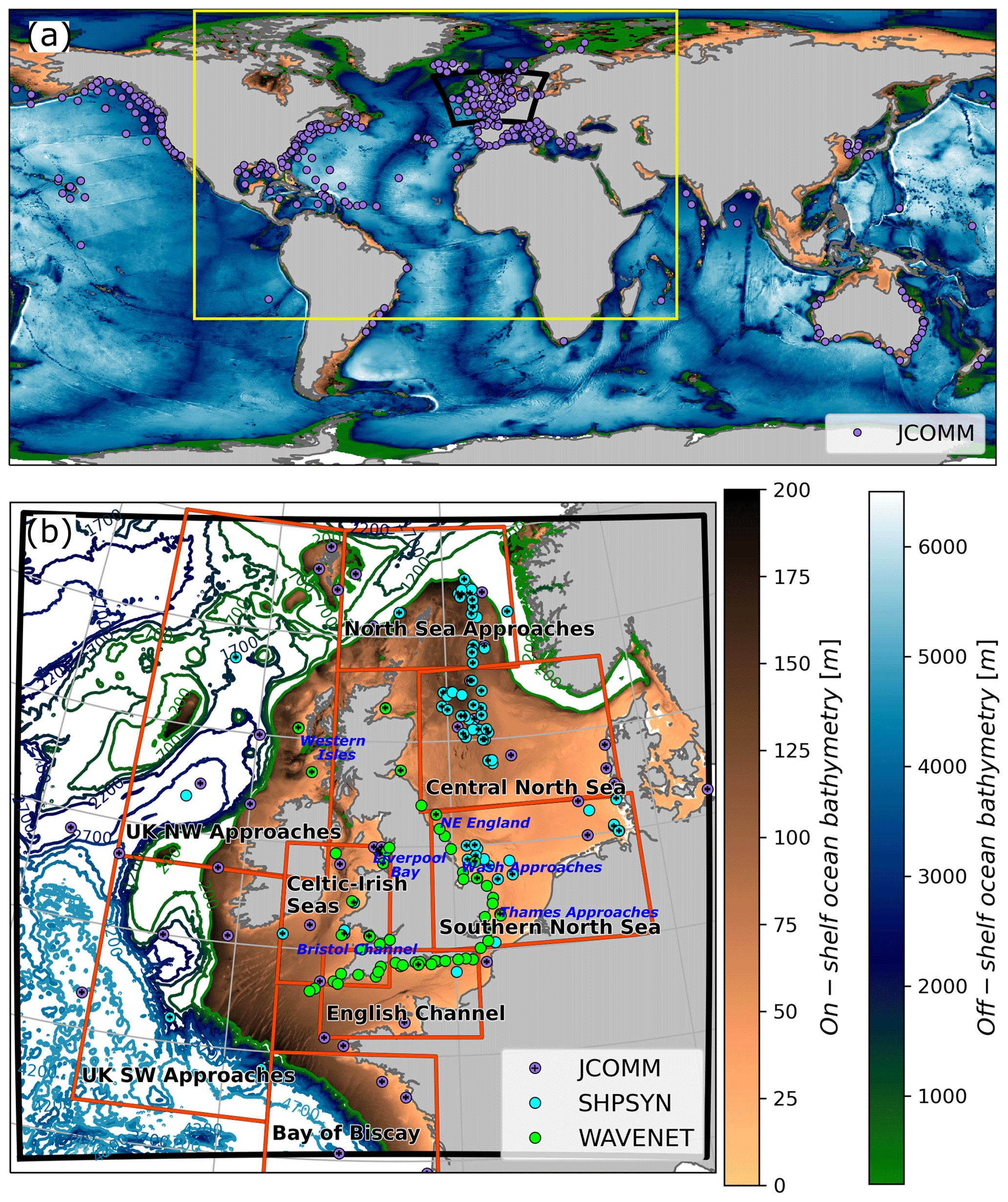
Figure 1(a) Global and (b) northwestern (NW) European shelf–UK waters physical context and model domains. The yellow box and solid black line in panel (a) indicate the cut-off area for the Atlantic wave ensemble and the NW European shelf–UK waters domains, respectively. (b) Domain of the NW European shelf–UK waters, with areas used for analysis indicated in red. In situ observations are shown as solid dots. In situ observations include the Joint World Meteorological Organization (WMO)/International Meteorological Organization (IMO) Commission for Oceanography and Marine Meteorology's (JCOMM) operational Wave Forecast Verification scheme (WFVS), Ship Synoptic Observations at fixed platforms (SHPSYN) and UK WAVENET and National Network of Regional Coastal Monitoring Programmes (NNRCMP) in situ observations for coastal waters (WAVENET). Locations at which there is overlap with JCOMM observations are marked with a cross.
2.1 Research to operations
All mission-critical NWP models at the Met Office are run under an operationally maintained supercomputer production system known as the Operational Suite (OS), which cycles model tasks in a dedicated, high-performance supercomputing environment. Since 2016, the Met Office's operational supercomputer has been a Cray XC40 comprising 6212 nodes of Intel Broadwell/Haswell processors, with up to 36 cores per node, connected by a high-speed Aries network. As of 2024, this system is due to be replaced by multiple Hewlett Packard Enterprise (HPE) Cray EX systems, which together will provide over 3000 nodes of Advanced Micro Devices (AMD) Milan processors, with 128 cores per node connected via a high-performance HPE Slingshot interconnect. At the time of writing, the operational GS512L4EUK model runs on 10 Broadwell nodes (360 PEs; processing elements), the AMM15SL2 deterministic on 8 nodes (304 PEs), the AMM15SL2 coupled on 62 nodes (252 PEs for the wave component; 1536 PEs for the ocean component) and the Atlantic ensemble on 2 nodes per member (72 PEs).
To maintain consistency and operational resilience, scientific and technical updates to these models follow a prescribed process defined in Parallel Suite (PS) projects, which aim to ensure the successful pull-through of scientific improvements of the Met Office's numerical weather prediction models into the operational environment. For the upstream NWP modelling systems, a PS is essentially a copy of the latest operational suite to which scientific and technical updates are applied. The PS is run in parallel with the current OS for a 6–8-week period, during which verification and performance metrics will be collected. The models described here correspond to the latest Met Office operational systems that became operational in May 2022 after PS45, run in parallel with OS44.
2.2 Model description
The Met Office operational wave forecasting system is based on the WAVEWATCH III® third-generation spectral model (Tolman, 2014), version 7.12. This model resolves the evolution of the phase-averaged two-dimensional (frequency–direction) wave energy spectrum in time and space, using the net effect of sources and sinks of wave energy; i.e. it is a total source term describing local wave energy growth and dissipation and advection of wave energy through the wave model grid. To enable conservation in the presence of ocean currents, the model describes these changes in terms of wave action (Ardhuin et al., 2012, 2017). The total source term is defined by the combination of different physical processes that, in deep waters, can be simplified to a wind–wave interaction term that describes the transfer of momentum from the atmosphere to the ocean surface waves, a nonlinear wave–wave interaction term that describes energy transfers between waves of different frequencies and a dissipation term describing the loss of energy from the waves to the surrounding ocean and atmosphere (Valiente et al., 2021a). Additionally, the operational system includes a linear input term used to initialise the wave growth and parameterisations of shallow water processes (i.e. depth-induced breaking (Sbrk) and wave bottom interactions (Sbf)). The total source term is therefore defined as follows:
WW3 provides multiple options for both source term parameterisations and numerical advection (WW3DG, 2019). This section summarises the options chosen for the Met Office operational configurations. More details of the compilation switches and source term tuning values can be found in the Supplement.
The Met Office operational wave forecasting system uses the Ardhuin et al. (2010) ST4 package to parameterise wave growth (Sin) and dissipation via whitecapping (Sdiss). The family of parameterisations in ST4 defines Sin, based on a WAM (Wave Model) cycle 4 parameterisation (Janssen, 2004), with an ad hoc reduction in the wind contribution to account for the impact of long waves on short waves through a tuneable sheltering coefficient (TAUWSHELTER = 0.3; refer to Table S2 in the Supplement) that decreases the drag coefficient at high winds (Saulter et al., 2017; Valiente et al., 2021a). For compatibility with Met Office Global Unified Model wind forecast data, a minor adjustment to the control of the input wind stress (BETAMAX namelist value set to 1.39; refer to Table S2 in the Supplement) has been implemented across both global and regional wave models. The BETAMAX value is also adjusted for the case of the ocean–wave regional coupled configuration, which is forced by European Centre for Medium-Range Weather Forecasts (ECMWF) winds (BETAMAX namelist value of 1.48; refer to Table S2 in the Supplement). Input wind stress to Sin is derived using conversion from the atmospheric model 10 m neutral wind speed to momentum stress flux computations, which are included in the source term (FLX0); i.e. stress is defined implicitly inside the source terms subroutines. The model assumes a neutral atmospheric stability in these calculations. Additionally, a switch with linear wave growth (LN1; Cavaleri and Rizzoli, 1981) for lower winds is implemented (Valiente et al., 2021b) to enable the consistent spin-up of the model from calm conditions and a more accurate description of the initial wave growth.
Sdiss is parameterised from the wave spectrum saturation following the ideas of Phillips (1985) with the integrations over directions presented in Ardhuin et al. (2010). The Discrete Interaction Approximation (DIA) package (NL1; Hasselmann et al., 1985) is used to resolve (Snl) nonlinear wave–wave quadruplets interactions that enable downshifting of energy input in the upper tail of the wave spectrum into longer waves. NL1 is developed for deep water, using the appropriate dispersion relation for resonant wave interactions. For shallow water, this source term uses a scaled version of the deep-water dispersion relation. As part of the shallow water physics, the Met Office wave model configurations include source terms to resolve depth-induced refraction, shoaling and breaking. Shallow water wave energy dissipation includes the surf-breaking parameterisation proposed by Battjes and Janssen (1978; DB1) and the JONSWAP (Joint North Sea Wave Project) bottom friction formulation (BT1; Hasselmann et al., 1973). Model spectral resolution is identical in all the wave operational systems, with 30 frequencies logarithmically spaced between 25 and 1.5 s (starting at 0.04118 Hz) and 36 directional bins that are linearly spaced.
Advection of wave energy through the model grid satisfies the wave dispersion relationship for which wave energy at lower frequencies will travel more rapidly through the model grid than waves at high frequencies. All configurations of the Met Office operational forecasting system utilise the SMC grid (Li, 2012). One of the key features of this grid is that it allows higher-resolution cells in areas of interest (shallow water, coastal areas and islands), while maintaining a coarse resolution in the open ocean for computational efficiency. The SMC grid retains the quadrilateral cells, as in the standard latitude–longitude grid, so that simple finite difference schemes could be used. Sub-time steps are applied on different cell sizes to speed up the propagation calculations with a choice of second- or third-order upstream non-oscillatory (UNO) advection schemes (Li, 2008). The refraction-induced wave spectral rotation and the great circle turning are combined and calculated with a remapping scheme, which is not subject to the Courant–Friedrichs–Lewy (CFL) restriction but to a physical limit not exceeding the bathymetry gradient direction or a user-defined limit angle. Grid cells are merged at high latitudes to relax the CFL restriction, and a fixed reference direction is used to define wave spectra in the polar region so that the whole Arctic Ocean could be included in the global domain. The multi-resolution refinement is useful to resolve small islands and coastline details, which are important in ocean surface wave propagations (Saulter et al., 2017). The Garden Sprinkler Effect (GSE), caused by the discrete directional bins of the wave energy spectrum, is alleviated with a diffusion term similar to the PR2 option in WW3 model (Booij and Holthuijsen, 1987), plus an optional averaging scheme for further smoothing (WW3DG, 2019).
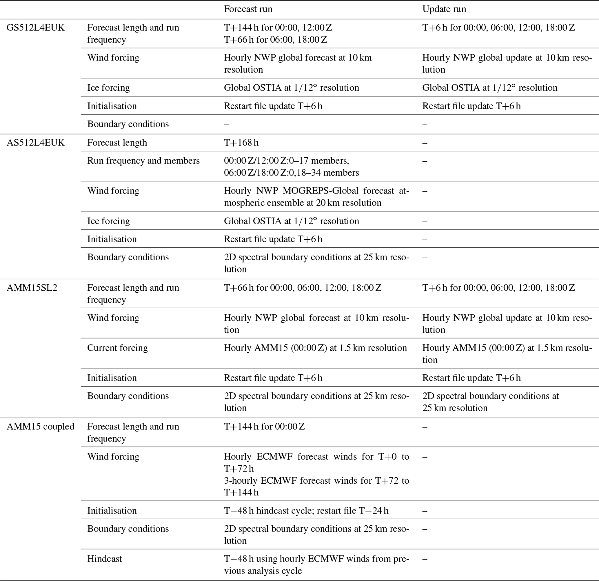
Table 1Specifications of the operational production of all the Met Office wave models, namely GS512L4EUK, AS512L4EUK, AMM15SL2 and AMM15 coupled. T refers to the forecast period with respect to the reference times at the 00:00, 06:00, 12:00 and 18:00 Z cycles.
2.3 Configurations of the operational forecasting system
2.3.1 GS512L4EUK global
The wave forecast global model configuration GS512L4EUK covers the globe from 80∘ S to 86∘ N (Fig. 1a), using model bathymetry based on the General Bathymetric Chart of the Oceans (GEBCO) 2014. The model grid is a four-tier SMC km refined grid, for which the coarsest cells are located in open waters and resolved at approximately 25 km (0.35∘ longitude by 0.23∘ latitude) at mid-latitudes. The 25 km cells represent a base resolution equivalent to an N512 atmosphere model and are successively halved to 12, 6 and 3 km as the grid comes closer to the coastline. An area of special interest is designated in UK waters, where higher resolutions are applied more widely (Saulter et al., 2016).

Figure 2Spherical multiple-cell (SMC) GS512L4EUK global model grid across the European–Arctic region. Coarsest (open waters) cells are resolved at approximately 25 km in the mid-latitudes (0.35∘ longitude by 0.23∘ latitude) and reduced by a factor of 2 to 12, 6 and 3 km. The 12 km cell sizes are set over the European region (27∘ N, 25∘ W to 68∘ N, 42∘ E), with a reduction to 6 km for cells with depths less than 320 m and to 3 km for those cells around the UK coastline.
Figure 2 shows the European–Arctic region of the GS512L4EUK global model grid. Over an Europe-wide region (covering approximately 25∘ W to 27∘ E and 42∘ N to 68∘ N), the coarsest cell size has been set to 12 km so that the model can exploit the full detail of the current Met Office global atmosphere–ocean model (approximately 10 km resolution), while any cells with depths less than 320 m are resolved at 6 km. This depth was chosen as a threshold to apply a higher resolution, since wave energy with mean periods of about 18 s or longer will begin to interact with the seabed. The use of the 3 km cell refinement is restricted to coastal cells on the NW European shelf (45∘ N, 16∘ W to 61.15∘ N, 9.4∘ E) to best represent the coastline of the UK (Saulter et al., 2016), while minimising computational costs. At higher latitudes, longitudinal cell sizes are doubled (by a factor of 2 at 60∘ N, 4 at 75∘ N and 8 at 83∘ N) in order to support a larger CFL time step than would be permitted by a regular latitude–longitude grid (Li and Saulter, 2014; Saulter et al., 2016). The Arctic part (cells inside the golden circle in Fig. 2) is not used in the operational forecast system at present, since it is covered by sea ice for most of the time.
The GS512L4EUK model is forced by hourly global atmospheric 10 m neutral wind files and ice concentration interpolated to the coarsest resolution of the SMC grid (i.e. 25 km). The 10 m neutral winds are provided by a high-resolution atmosphere–ocean coupled global configuration (Williams et al., 2018) of the Unified Model (UM; e.g. Walters et al., 2019; Brown et al., 2012) and NEMO (Nucleus for European Modelling of the Ocean) each hour; the atmosphere–ocean coupled model has 0.23∘ longitude by 0.16∘ latitude resolution (N1280L70; 2560 latitude × 1920 longitude and 70 vertical levels), with approximately 10 km grid length in the mid-latitudes. Ice concentration is provided by the Operational Sea Surface Temperature and Sea Ice Analysis (global OSTIA; Good et al., 2020), which is also produced at the Met Office. GS512L4EUK uses simple ice blocking (IC0), where grid points covered by ice are treated as land, and a cut-off ice concentration value of 50 %. This global model provides full 2D spectral boundary conditions for the nested operational wave (AS512L4EUK; AMM15SL2–UK waters) and AMM15 ocean–wave coupled configurations.
2.3.2 AS512L4EUK Atlantic ensemble wave model
The Atlantic ensemble forecast system for prediction of Atlantic–UK wind waves (AS512L4EUK; Bunney and Saulter, 2015; Saulter et al., 2016) is based on a cropped version of the GS512L4EUK grid from 25∘ S to 83∘ N. Forcing conditions include hourly winds from the Met Office Global and Regional Ensemble Prediction System global (MOGREPS-G) and ice concentration from global OSTIA. MOGREPS-G is an atmosphere–ocean coupled model of N640L70 resolution with 1280 latitude × 960 longitude and 70 vertical levels, which is equivalent to approximately 20 km grid length in the mid-latitudes. MOGREPS-G includes 18 ensemble members, with 1 control member and 17 perturbed members. Post-processing lags the two most recent two cycles to provide probability forecasts from an ensemble of 36 members (34 perturbed + 2 control). For additional information on AS512L4EUK, refer to Bunney and Saulter (2015).
2.3.3 AMM15SL2 NW shelf–UK waters
AMM15SL2 is the baseline configuration used for the UK waters' wave-only model and the AMM15 ocean–wave coupled model. The AMM15SL2 configuration covers the NW Shelf–UK area from approximately 45∘ N, 20∘ W to 63∘ N, 12∘ E, with a resolution of 3–1.5 km. The domain extends beyond the shelf break in order to include boundary conditions in open waters, which are not subject to shallow water processes but are primarily focused on forecasting the shelf seas around the UK (i.e. Celtic and Irish seas, North Sea and English Channel; Fig. 1b). The AMM15SL2 configuration name is derived from the AMM15 (1.5 km NW shelf Atlantic Margin model) ocean model that encompasses the same region and the use of a two-level SMC grid refinement (Li, 2011), with a variable resolution based on both proximity to the coast and water depth (Saulter et al., 2017; Valiente et al., 2021b). The grid resolution is of 3 km for water depths larger than 40 m and 1.5 km for coastal cells with water depths of less than 40 m (Fig. 2). The SMC grid is based on a rotated North Pole at 37.5∘ N, 177.5∘ E, achieving an evenly spaced mesh around the UK. Bathymetry and coastal masking for this configuration are the same as the 1.5 km AMM15 NEMO-based (Madec and the NEMO team, 2016) ocean configuration (Tonani et al., 2019; Graham et al., 2018). Both bathymetry and land–sea masks are based on the European Marine Observation and Data Network (EMODnet portal; September 2015 release) corrected to mean sea level (Tonani et al., 2019).
AMM15SL2 wave-only is driven by hourly NWP 10 m neutral winds from the global UM-NEMO operational system and is also forced by hourly currents from the regional AMM15-FOAM ocean–wave coupled model shelf seas forecast assimilation model (Tonani et al., 2019) interpolated in time and space to the underlying 3 km cell resolution regular grid version of the SMC. The coupled version of this configuration differs from the AMM15SL2 UK waters' wave model in the forcing sources, which is driven by hourly surface (10 m) wind data at approximately 9 km resolution provided from the atmospheric high-resolution global configuration of the Integrated Forecast System (IFS) run at the European Centre for Medium-Range Weather Forecasts (ECMWF; https://www.ecmwf.int/en/forecasts/documentation-and-support, last access: 15 December 2022). The wave model is two-way-coupled to the ocean NEMO model AMM15-FOAM using the Ocean–Atmosphere–Sea Ice–Soil Model Coupling Toolkit (OASIS-MCT; Valckle et al., 2015) coupling libraries. The wave model passes the wave-modulated waterside stress, significant wave height, mean wave period and Stokes drift to the ocean component, and surface currents are passed from ocean to wave. The ocean component integrates a NEMO physical ocean model and the NEMO variational data assimilation software (NEMOVAR; e.g. King et al., 2018; Waters et al., 2015). NEMOVAR uses a 3D-Var first guess at appropriate time (FGAT) scheme, which includes a bias-correction scheme for both sea surface temperature and altimeter data. For additional information on the AMM15 coupled model, refer to Tonani et al. (2019) and Bruciaferri et al. (2021).
2.4 Operational production
Operationally, GS512L4EUK and AMM15SL2 wave models run four cycles per day (00:00, 06:00, 12:00 and 18:00 Z; Table 1) to T+66 h. The 00:00 and 12:00 Z cycle on each day are extended to a 144 h forecast for GS512L4EUK. Both GS512L4EUK and AMM15SL2 are initialised using the restart file T+6 h from a short 6 h update cycle, using the most up-to-date NWP winds. In this way all models provide a forecast that it is initialised with the best available descriptions for atmosphere and ocean (i.e. with as many observations assimilated as possible). Ice concentration from global OSTIA for GS512L4EUK, and currents from AMM15-FOAM for AMM15SL2 wave are updated once a day at 00:00 Z. The AMM15SL2 wave at 00:00 Z runs before the ocean–wave coupled AMM15 00:00 Z in the Met Office production cycle, forcing this cycle to use the forecasted currents from the previous day's AMM15 ocean–wave model cycle (i.e. currents at T+24 h from the previous cycle of AMM15 coupled). The AMM15 ocean–wave coupled model runs once a day, triggering a 144 h forecast. Each model cycle starts with a T−48 h hindcast prior to each forecast. Refer to Saulter et al. (2020) and Tonani et al. (2022) for more information on the production cycle of the Copernicus Marine Environment Monitoring Service (CMEMS) AMM15 ocean–wave coupled model.
The AS512L4EUK wave ensemble currently runs as a lagged ensemble, in which members 0 to 17 run to full length (168 h) at 00:00 and 12:00 Z, whereas members 0 and 18 to 34 run at 06:00 and 18:00 Z. A full 36 member lagged ensemble is made up at each cycle from the overlapping full length members.
Modelled waves and winds are evaluated using the significant wave height (Hs), mean zero up-crossing period (T02) and mean wave direction (Dir) for the waves and 10 m height wind speeds (U10) and wind direction (U10 dir) for the wind forcing conditions. These parameters are widely used for model evaluation, as they give information concerning the wave model performance in aspects such as bulk energy imparted to the ocean surface waves and representation of the wave energy distribution through the frequency domain and directional space (Saulter, 2020).
Wave parameters from the model simulations are assessed using the following four different datasets: (i) in situ data every h from the Joint World Meteorological Organization (WMO)/International Meteorological Organization (IMO) Commission for Oceanography and Marine Meteorology's (JCOMM) operational Wave Forecast Verification Scheme (WFVS; Bidlot et al., 2007), hereafter JCOMM-WFVS, for Hs and T02; (ii) hourly Daily Ship Synoptic Observations at fixed platforms for Hs and T02 across the NW shelf, hereafter SHPSYN; (iii) hourly UK WAVENET and National Network of Regional Coastal Monitoring Programmes (NNRCMP) in situ observations for coastal waters comprising a Waverider buoy measuring Hs, T02 and Dir, hereafter WAVENET; and (iv) global satellite-merged altimeter data (hereafter MA_SUP03) including Jason-2, CryoSat and SARAL (Satellite with ARgos and ALtiKa) Hs data. Wind forcing conditions (U10 and U10 dir) are verified using the JCOMM-WFVS, SHPSYN and MA_SUP03 datasets.
Basic metrics for model evaluation are described in the Supplement. These include bias, root mean square deviation (RMSD), observations (SDobs) and model standard deviation (Sdmodel), Pearson correlation coefficient (Pearson's r), standard deviation of the error (SdE), covariance (Cov) and variance (Var). Extreme verification and extra metrics for model evaluation are also provided and include scatter index (SI) and symmetric slope (SS) between the model and the observations. SI is calculated by dividing the standard deviation of model–observation differences and SDobs. The SS is described as the ratio of model variance to observations variance. Bias and RMSD are used to document the forecast accuracy, whereas all the metrics are presented for the model evaluation.
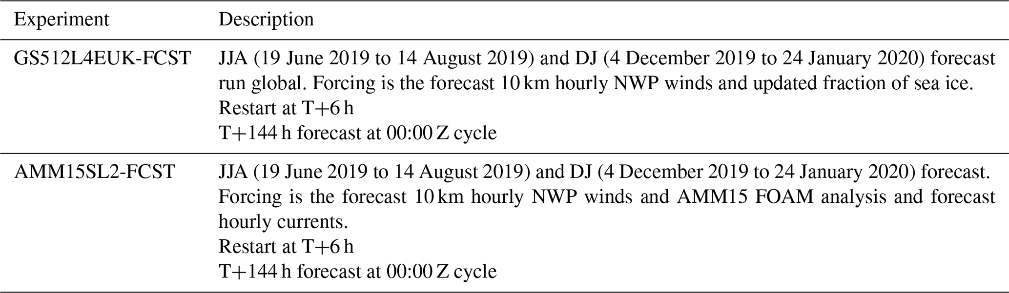
The quality of the Met Office short-range forecasting system is evaluated by running and verifying the two baseline global (GS512L4EUK) and regional (AMM15SL2) UK waters' (refer to Fig. 1a, b) configurations during 50 d in summer (from 19 June 2019 to 14 August 2019; June–August, JJA) and winter (4 December 2019 to 24 January 2020; December–January, DJ). These experiments (Table 2) replicate the operational configurations described in Sect. 2.3. Initial conditions for forecast experiments used the corresponding T+6 h restart output file generated during the analysis experiments (previously run). For comparison purposes, AMM15SL2-FCST was run up to T+144 h, as per GS512L4EUK-FCST, as opposed to T+66 h used in operations. It is noted that currents used as forcing were not available in the last 78 h of the AMM15SL2-FCST runs.
The forecast skill, from T+24 to T+144 h, of wind and wave parameters across the NW shelf area over the summer months of JJA and the winter months of DJ for the two baseline configurations is presented in Fig. 3. Winds tend to be overestimated in both configurations during most of the forecasting period up to T+96 h (GS512SL4EUK and AMM15SL2 biases are 0.4–0.6 and 0.1–0.3 m s−1, respectively; Fig. 3a). At longer forecast lead times, winds appear to be slower versus the first forecast days, and the tendency is to show a reduced bias that might be also associated with compensating errors (biases = 0.1 and −0.2 m s−1 for GS512SL4EUK and AMM15SL2 at T+144 h). This is also observed in Hs biases, where values are also slightly overestimated (biases = 0.1 and 0.2 m for GS512SL4EUK and AMM15SL2), and model–observation differences are smaller during the winter months (0.02 and 0.1 m for GS512SL4EUK and AMM15SL2, respectively; Fig. 3c).
Despite the bias reduction observed in U10 and Hs, the forecast skill of both configurations decreases with lead time (i.e. positive trend) and is slightly weaker during the winter months for both forcing and wave bulk parameters (i.e. U10, U10 dir, Hs and T02), suggesting a consistent behaviour across model resolution. The decrease in the forecast skill appears to be relatively steady for the first 4 d of forecast (U10 RMSD = 1.5–2.5 m s−1 and Hs=0.1–0.4 m up to T+96 h in JJA; Fig. 3b, d); however, the RMSD trend indicates a more rapid decrease in the forecast skill after these (increases to 3.5 m s−1 and 0.6 m at T+144 h). It is noted that the degree of decrease in the forecast skill for the case of T02 is smaller compared with Hs, and in fact, values of both bias (−0.8 and −0.5 s for GS512SL4EUK-FCST and AMM15SL2-FCST, respectively; Fig. 3g) and RMSD (1.4 and 1.1 s for GS512SL4EUK-FCST and AMM15SL2-FCST, respectively; Fig. 3h) are almost constant for the first 4 d in both JJA and DJ periods (Fig. 3g, h).
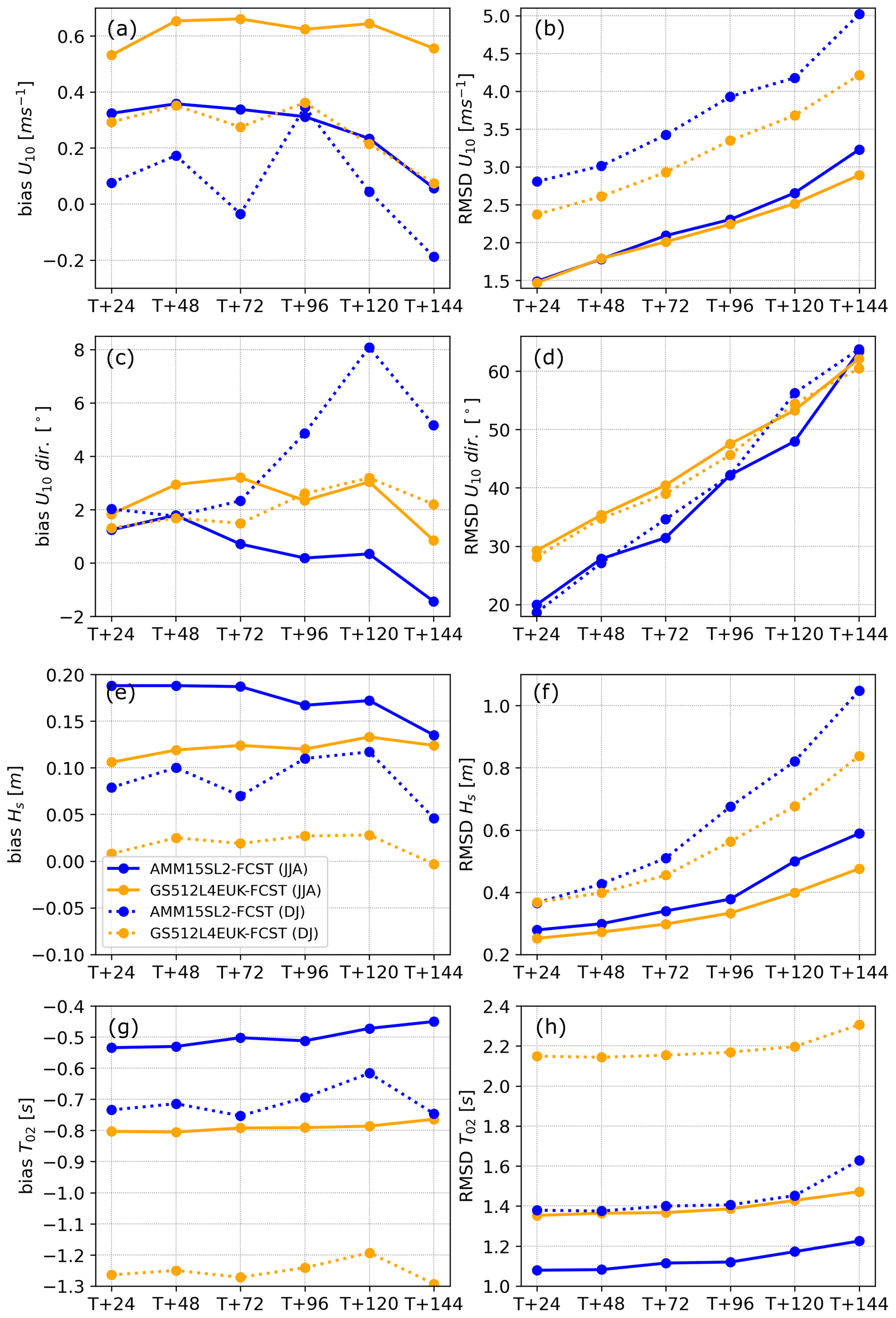
Figure 3Forecast (a, c, e, g) bias and (b, d, f, h) root mean square deviation (RMSD) for wind speed (U10; a, b), wind direction (U10 dir; c, d), significant wave height (Hs; e, f) and mean period (T02; g, h) every 24 h over a forecast period of 6 d (T+144 h) for the area of the NW shelf. Values are averaged over the months June–August (JJA; solid lines) and December–January (DJ; dotted lines) and correspond to the NW shelf–UK waters model (AMM15SL2-FCST; blue) and the global model (GS512L4EUK-FCST; orange).
Model forecast skill for Hs suggests that the positive impact of including the surface currents and having increased resolution is not always shown in the overall statistics. Indeed, Hs bias and RMSD for the regional baseline configuration during the forecast period are greater (AMM15SL2-FCST RMSD = 0.3–1 m) than for the global (GS512SL4EUK-FCST RMSD = 0.2–0.8 m) model (Fig. 3d). Conversely, AMM15SL2-FCST shows a better performance with a decrease in bias and >20 % reduction in RMSD compared to the global configuration for T02 (Fig. 3g, h). Forecast skill differences are associated with a better representation of the bathymetric features, depth-related processes and wave–current interaction present in AMM15SL2. The overall contribution of each of these factors is investigated in the next section.
The focus of this paper is to evaluate some of the physical aspects of our operational system in detail. An assessment of the forecast performance showed that the model has a consistent behaviour across lead times, with a degradation in performance that is mostly explained by the wind forcing. We now investigate the performance characteristics of the baseline configurations, with a specific focus on the influence of spatial resolution and wave–current interactions using long analysis runs (-AN), herein GS512L4EUK-AN and AMM15SL2-AN (Table 3). Trials covered the period from 1 January 2019 to 31 December 2020 and were based on daily cycles of the models forced by NWP 10 km resolution hourly operational winds, between T+0 and T+6 h (four cycles per day), OSTIA sea ice fraction (GS512L4EUK-AN) and AMM15 FOAM 1.5 km sea surface currents (AMM15SL2-AN). The trials were initialised from rest with a 10 d spin-up period that was discarded. Lateral wave spectral boundary conditions for the AMM15SL2-AN simulation were supplied by the GS512L4EUK-AN simulation. For a detailed evaluation of AMM15 ocean–wave coupled model and AS512L4EUK wave ensemble, refer to Saulter (2020), Bruciaferri et al. (2021), and Bunney and Saulter (2015), respectively.

5.1 Global spatial and temporal model accuracy
Global spatial and temporal forcing accuracy is evaluated using the altimeter MA_SUP03 data (Fig. 4), which provides measurements of wind speed and wave height. The main feature is that there is an underestimation of observed wind speeds by the model (Fig. 4c, d) in those areas that present either small or strong mean wind speeds (Fig. 4a, b), while overestimation occurs in the mid-latitude regions with modal observed mean wind conditions (5–10 m s−1). Areas which present the lowest mean wind conditions are those across equatorial and close mid-latitude regions with very small wind variability (SD mean values are of O. 0.6 m s−1; Fig. 4g, h). Underestimation in these areas seems to be partially linked to sampling bias from the satellite for calm wind conditions. Additionally, very energetic areas such as the southern part of the Pacific Ocean also present negative bias throughout the year, but these are more exacerbated during JJA months (Fig. 4c; winter in the Southern Hemisphere), during which the largest mean winds are registered. Equally, negative bias is present in the northern part of the Atlantic Ocean also corresponding to the strongest winds (average U10>10 m s−1) during DJF (December–February) Northern Hemisphere winter months (Fig. 4d). As expected, these areas with the strongest winds also present the largest SDmodel (>2 m s−1) and RMSD (1.2 m s−1).
The variability in wave metrics match the variability in the wind field, such that larger values of bias, RMSD and SDmodel always correspond with areas with the strongest average wave conditions. A bias seasonality is observed with waves underestimated across areas affected by tropical and intra-tropical storms (i.e. tropical, mid- and high latitudes in the Northern Hemisphere during DJF; Fig. 5b, d, f, h) and Indian Ocean during JJA (Fig. 5a, c, e, g). This negative bias during stormy seasons turns into a positive one of the same order during periods with calmer average conditions (Fig. 5c, d). Conversely, the southern part of the South Pacific Ocean shows a large variability in the bias, with no clear seasonality, possibly due to compensating errors. Hs values of RMSD oscillate between 0.1–0.3 m in most parts of the globe, with a substantial increase to 0.5–0.6 m in those areas, with the largest mean wave conditions and variability about the mean values (i.e. Southern Ocean during JJA and North Atlantic and North Pacific during DJF). Additional large positive biases around island chains and ice edges are also present, which we attribute to a combination of misrepresentation errors from the observations and model. On the one hand, it is acknowledged that satellite measurement errors are larger in complex coastlines, and on the other hand, model resolution and misplacements in the extension of ice sheets will yield in position errors in the wave field. Adopting the GS512L4EUK SMC configuration helped reduce such biases compared to previous configurations (Saulter et al., 2016); however, biases in these areas are still likely due to issues with land/ice masking and the representation of fetch in the model grid.
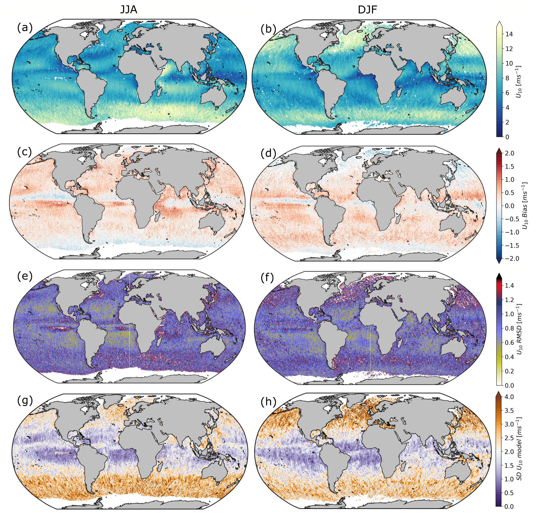
Figure 4(a, b) Mean, (c, d) bias and (e, f) root mean square deviation (RMSD) between wind (U10) forcing conditions and merged altimeter observations (MA_SUP03) and (g, h) model standard deviation (SDmodel) across the global domain for GS512L4EUK-AN. Statistics are aggregated every 15 d and averaged for JJA (left column) and DJF (right column).
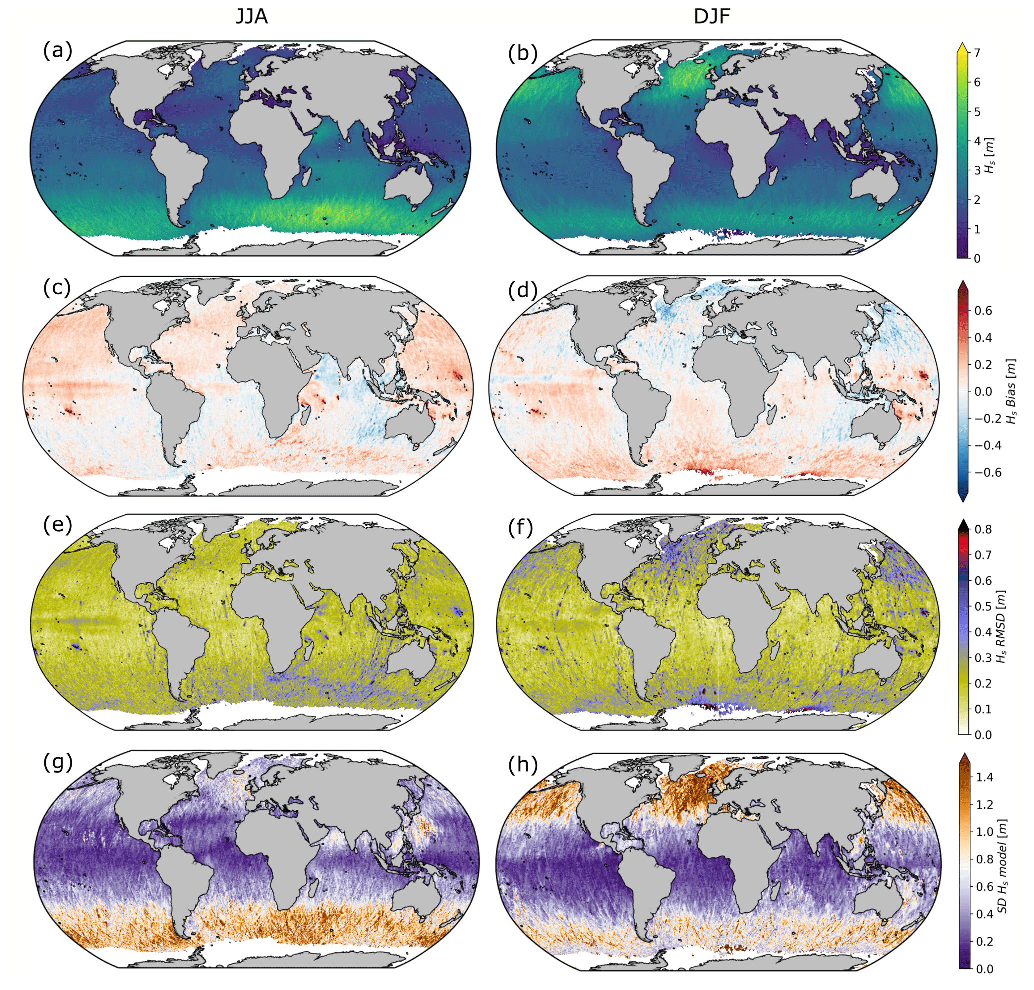
Figure 5(a, b) Mean, (c, d) bias and (e, f) root mean square deviation (RMSD) between modelled significant wave height (Hs) and merged altimeter observations (MA_SUP03) and (g, h) model standard deviation (SDmodel) across the global domain for GS512L4EUK-AN. Statistics are aggregated every 15 d and averaged for the months JJA (left column) and DJF (right column) over 2019–2020.
Model calibration is based on the best overall performance skill. Figures 4 and 5 suggest some imbalance during swell-dominated conditions in areas such as the Southern Pacific Ocean and the Indian Ocean, where winds over this period appear overpredicted, whereas significant wave height is consistently underestimated (e.g. waters approaching western part of Australia; Fig. 5c, d). Something similar, albeit to a lesser extent, occurs in the tropical and mid-latitudes in the western part of the North Atlantic, where, despite a slight overestimation of the forcing conditions, the model shows a negative bias with respect to altimeter observations.
5.2 Regional spatial and temporal model accuracy
An assessment of AMM15SL2-AN-modelled Hs and T02 against in situ observations across the UK waters is presented in Fig. 6. Analysing in situ observations individually allows us to obtain a more detailed understanding of the caveats for the model performance in the different areas of analysis. Although some metrics vary between summer and winter months, overall, T02 seems to be consistently underestimated in most locations (bias = −0.5 s; Fig. 6g, h), whereas Hs is slightly overestimated (bias = 0.1–0.2 m, Fig. 6e, f). Following the seasonal pattern observed in the global domain, AMM15SL2 model performance is slightly weaker (i.e. larger values of bias and RMSD) when waves are larger (i.e. DJF). However, conversely to the other metrics, the correlation between model and observations (r) is improved during the winter months (average r>0.92 versus 0.88 during JJA), suggesting that AMM15SL2 struggles more to replicate the wave energy in the frequency domain during lower-energy conditions (Hs=1–2 m, T02=5–6 s; Fig. 6a–d). Spatially, there are some specific locations where mean bias, RMSD and SdE statistics are consistently large throughout the year (e.g. buoys in the Bristol and English channels and coastal buoys in very sheltered areas). While the model shows some skill in these regions, the high variability characterised by strong currents due to the tidal range (hypertidal in the case of the Bristol Channel), linked to the fact that those locations are very close to the coast and some local features (e.g. headlands; highly spatially variable bathymetry with features of <3–1.5 km spatial scale), are not fully represented by the model, which make these regions very dynamic and difficult to resolve more accurately with the current model configuration.
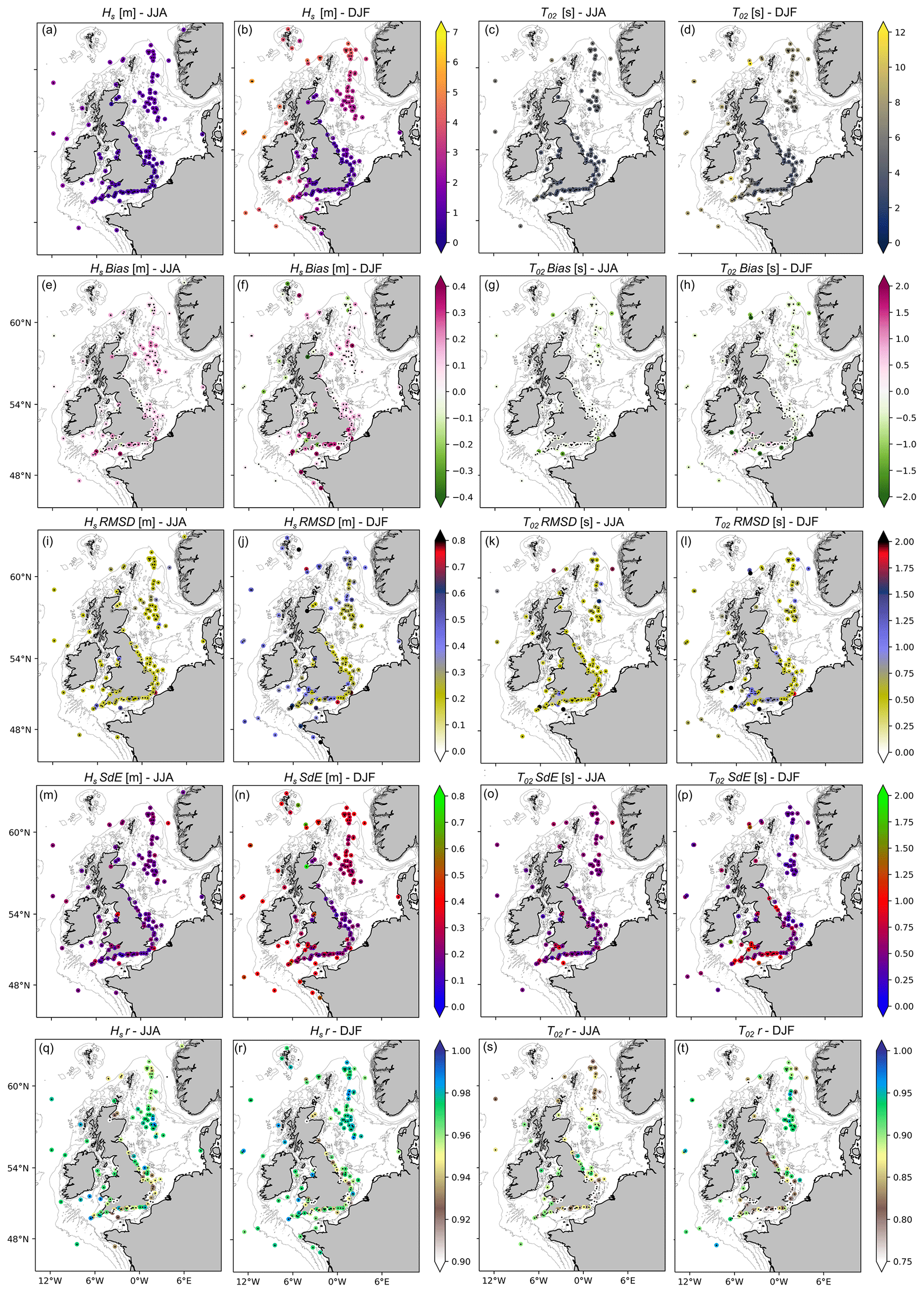
Figure 6(a–d) Mean, (e–h) bias, (i–l) root mean square deviation (RMSD), (m–p) standard deviation of error (SdE) and (q–t) Pearson correlation coefficient (r) between modelled significant wave height (Hs) and mean zero up-crossing period (T02) and in situ observations across the UK waters' domain for AMM15SL2-AN. Statistics are computed for the months of JJA (left column) and DJF (right column) over 2019–2020. Observations included are JCOMM-WFVS, SHPSYN and WAVENET.
5.3 Comparison of configuration performance
The relative importance of wind and current inputs is presented through evaluations comparing GS512L4EUK-AN and AMM15SL2-AN trials against all observations (i.e. WAVENET, JCOMM-WFVS, SHPSYN and MA_SUP03; Table 4). Overall metrics are computed for the individual domains (i.e. the entire globe and the NW shelf–UK waters area, respectively). Note that evaluation of wave direction (Dir) only corresponds to the coastal waters of the UK.
Table 4Summary statistics for wind speed (U10), wind direction (U10 dir), significant wave height (Hs), mean zero up-crossing period (T02) and wave direction (Dir), including GS512L4EUK-AN and AMM15SL2-AN versus observations of WFVS, SHPSYN, WAVENET and merged altimeter (MA_SUP03) over 1 January 2019 to 31 December 2020.
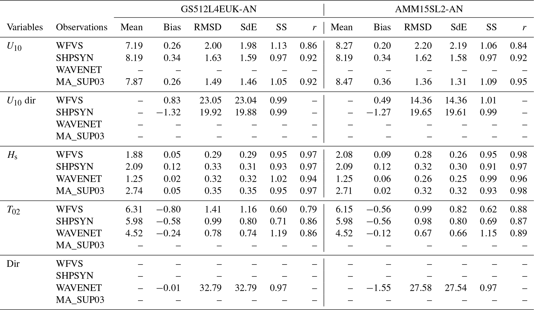
One of the main factors that influence the reliability of a wave spectral model is the accuracy of the forcing conditions. Modelled wind forcing is compared against observations in order to assess their consistency for the baseline configurations (Table 4). Interestingly, differences in U10 metrics are not significant, indicating that wind forcing conditions are steady and suggesting that the wind interpolation to the underlying regular grid with the coarsest SMC resolution (25 km for GS512L4EUK and 3 km for AMM15SL2) does not degrade the overall wind speed performance. However, U10 dir compares closer to observations for the AMM15SL2 domain (RMSD = 21.49 and 17.00∘ and SdE = 21.46 and 16.98∘ for GS512L4EUK and AMM15SL2, respectively), demonstrating that errors between modelled U10 dir and observations are both smaller and more representative of the wind conditions across the NW shelf (i.e. when the original spatial variability in the 10 km winds is retained and not upscaled).
The incorporation of ocean surface currents in the wave model aims to improve modelled sea states (e.g. Hersbach and Bidlot, 2008; Palmer and Saulter, 2016; Ardhuin et al., 2017; Alday et al., 2022). When analysing the observations as a whole (average values), the statistics show excellent model accuracy for predicting Hs, even when currents are not included (i.e. GS512L4EUK). Both baseline configurations present very good correlation coefficients (Hs r=0.94–0.97 and T02 r=0.84–0.88 for GS512L4EUK-AN and AMM15SL2-AN, respectively; Table 4), mean SS (0.95–0.96; i.e. SDobs is larger than Sdmodel) and small positive biases for Hs (0.06 and 0.07 m) and negative for T02 (bias = −0.54–0.41 s). When comparing the differences in performance only for the NW shelf–UK waters (Fig. 7), the results show that although there is a positive impact of the surface currents and increased resolution, with 5 % mean square error (MSE) decrease in coastal locations (i.e. WAVENET; Fig. 7), this is not always present in the overall statistics of Hs, and neutral changes and even some degradation exist in specific locations (overall 1 % and 5 % increase in MSE and bias).
The increased resolution in AMM15SL2, together with the refraction produced by tidal currents, help to better capture the mean period and wave direction near the coast where bathymetric changes and coastal obstructions are better resolved (Fig. 7). AMM15SL2-AN shows an acceptable performance in all the coastal areas of analysis, with Dir RMSD values oscillating from 17 to 32∘, which corresponds to 25 % of the observation standard deviation. This percentage in the RMSD increases to 36 % for the case of GS512L4EUK-AN. A further contribution to the improved wave direction fields in AMM15SL2 is also expected from the wind interpolation. Model accuracy improvement for T02 is more than 2 %–9 % on average for MSE and bias (Table 4), with >20 % reduction in RMSD. This overall improvement in the mean period for AMM15SL2-AN is even more significant in most coastal locations, despite some exceptions, such as the Scarweather directional wave buoy (Bristol Channel), where although the tidal modulation of the wave field is only captured by AMM15SL2-AN, it leads to a larger spread in the observation–model differences.
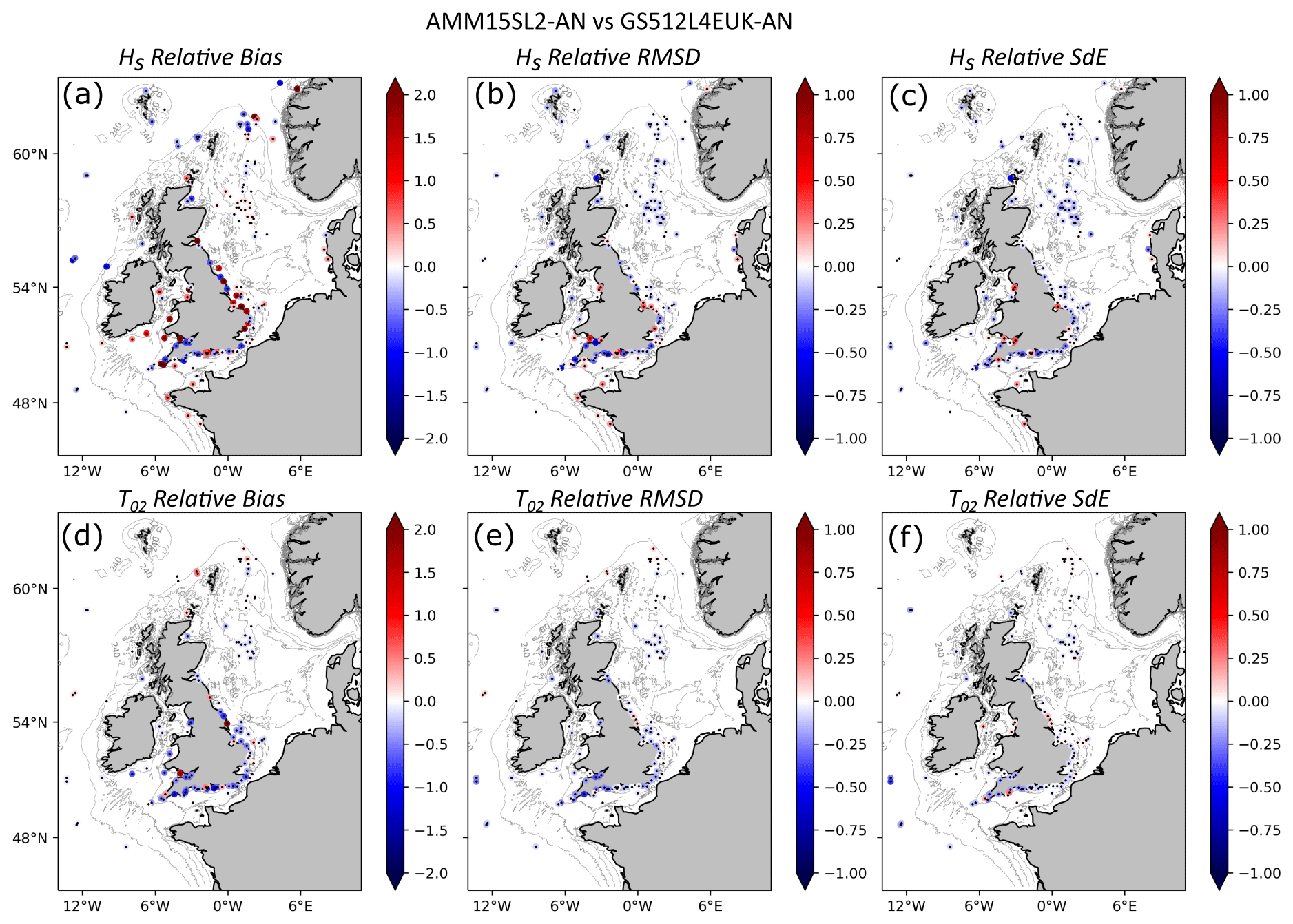
Figure 7Relative change in (a, d) absolute bias, (b, e) RMSD and (c, f) SdE between observation–model comparison for AMM15SL2-AN and GS512L4EUK-AN for significant wave height (Hs) and mean period (T02) across UK waters. Statistics are computed over 2019–2020, and the observations included are JCOMM-WFVS, SHPSYN and WAVENET. Negative (positive) values indicate a reduction (increase) in the metric by AMM15SL2-AN. To facilitate visualisation when no relative change is observed, all in situ locations are indicated with a black dot.
5.4 Wave–current interaction
The addition of surface currents has effects on wave generation, advection and refraction, with the latter being one of the main wave–current processes affecting the wave field in areas with large tidal currents such as those on the shelf. We focus now on areas where the tide has a dominant effect on the wave field using WAVENET in situ directional wave buoys.
When comparing GS512L4EUK and AMM15SL2, we show that wave–current interaction in areas where tidal currents are important produces larger wave heights and positive changes in the wave period and direction. An example of these fluctuations is presented at Start Bay Waverider (Fig. 8), which is a tide-modulated coastal in situ location in the English Channel. Adding the wave–current interactions leads to a reduction in the small negative Hs bias at this site from −0.11 to −0.02 m, with a reduction in the RMSD from 0.2 to 0.14 m. The quantile–quantile relationship (QQ) for Hs at this location shows that both configurations are in very good agreement with observations (r=0.95 and 0.97 for GS512L4EUK-AN and AMM15SL2-AN, respectively) and that both tend to underestimate the tail of the distribution; however, this is much closer to observations in AMM15SL2-AN. T02 QQ shows an underprediction of the lower periods (T02=2–6 s with bias = 0.5–1 s; Fig. 8c, d) and a significant overestimation of larger periods (T02>8 s) that is accentuated in the regional configuration. Despite this, overall T02 metrics are improved when currents are accounted for. In line with the improvement of Dir by AMM15SL2-AN present in most coastal locations, Dir RMSD at Start Bay is significantly reduced from 44 to 32.25∘, and this is reflected in a significant reduction in the model biases.
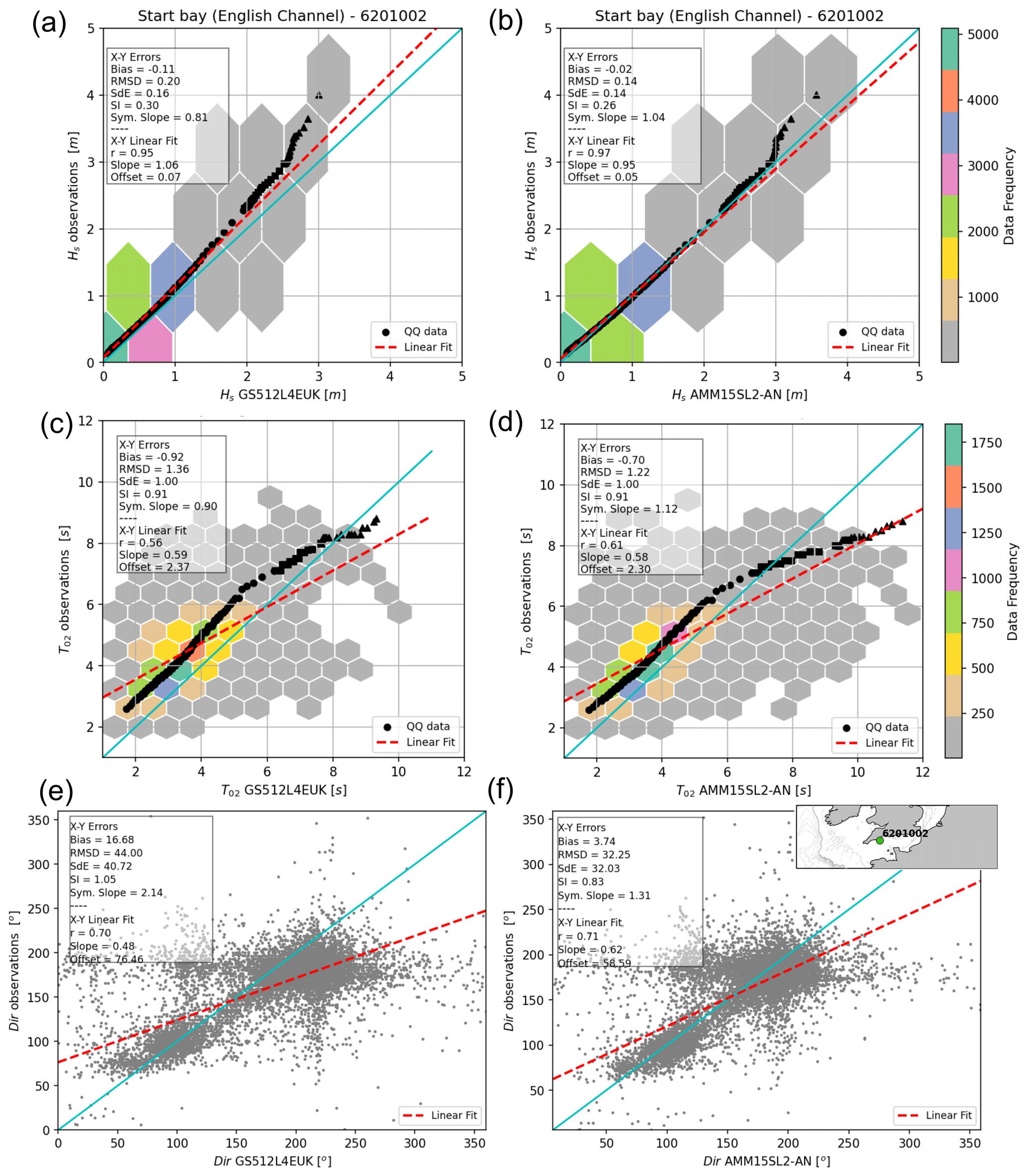
Figure 8(a, b) Significant wave height (Hs) and (c, d) mean period (T02) quantile–quantile relationship and scatter data for GS512L4EUK-AN (a, c, e) and AMM15SL2-AN (b, d, f) at the Start Bay in situ wave buoy. (e, f) Scatterplots for wave direction (Dir) at Start Bay in situ wave buoy. The inset with the wave buoy location is presented in panel (f). Wave bulk statistics are included in each individual panel and correspond to the comparison between model and observations over 1 January 2019 to 31 December 2020.
Tidal modulation of the wave field is observed in several locations. As an example that is representative of most coastal areas, Fig. 9 shows the time series of Hs, T02 and Dir for both configurations at the Scarweather wave buoy, located in the Bristol Channel, where an increase in the observed T02 and Hs can be seen during each tidal cycle (Fig. 9a, b). This modulation is only present in the AMM15SL2 configuration; however, sometimes a lag in the tidal fluctuation (3 h for Scarweather; up to 6 h in other locations) occurs between the model and observations that may lead to poorer metrics than when no currents are used (i.e. the run without currents provides a smoother signal). In line with an additional forcing evaluation of the current field (refer to the Supplement), this lag is linked to the negative veering (tidal phase) that is present in the modelled currents where observations tidal velocities lead the model velocities. Equally, we also noted the importance of the tidal modulation on the wave direction present in AMM15SL2-AN time series captured on the observations within a range of ±30∘ (Fig. 9c) in these coastal wave buoys.
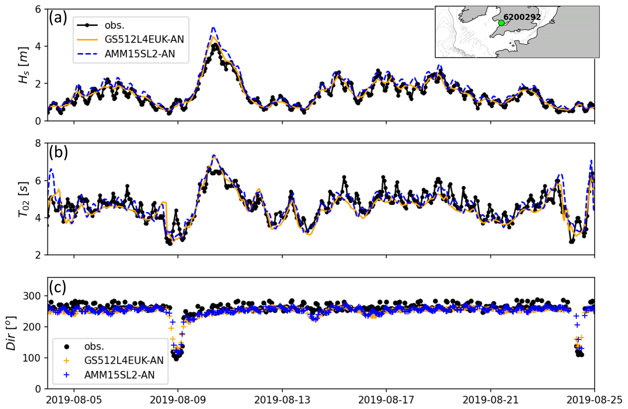
Figure 9Time series of (a) significant wave height (Hs), (b) mean period (T02) and direction (Dir) for GS512L4EUK-AN and AMM15SL2-AN (right column) at the Scarweather in situ wave buoy. The inset with the wave buoy location is presented in panel (a).
Differences in the accuracy of both configurations suggest that wave refraction and shifts in the relative frequency are better captured with the addition of the sea surface currents in most of the domain. However, overall metrics for Hs are slightly weaker in certain areas of analysis such as the Irish and Celtic seas, English and Bristol channels and eastern coast of England. To isolate the effect of currents and not account for any differences in resolution, we run the AMM15SL2 configuration without currents during August 2019 and compare model differences in Hs over two tidal cycles during spring tides (Fig. 10a). Positive residual differences in Hs correspond to those locations, where AMM15SL2 presents some degradation with respect to GS512L4EUK. A model evaluation showed that both configurations tend to slightly overestimate Hs; therefore, the overall positive bias is exacerbated by the contribution of the residual currents in AMM15SL2. Additionally, the evaluation of the currents effects on the wave energy distribution in two different shallow coastal locations demonstrates that including tidal currents produces a consistent shift towards longer periods (Fig. 10e, g), thus reducing the energy bias between model and observations at low frequencies (not shown), hence leading to a better agreement for the period in AMM15SL2. In terms of Dir, model differences during ebb (Fig. 10b) and flood (Fig. 10c) tide conditions show wave refraction angles of ±10∘ when currents are included, helping to better capture the distribution of the wave energy in the directional space (e.g. Fig. 8f). This suggests that AMM15SL2 captures the distribution of the energy in terms of frequency and direction better, whereas the total energy might sometimes be too large in this configuration. In other words, the bulk energy imparted to the ocean surface waves might be excessive during low–moderate conditions.
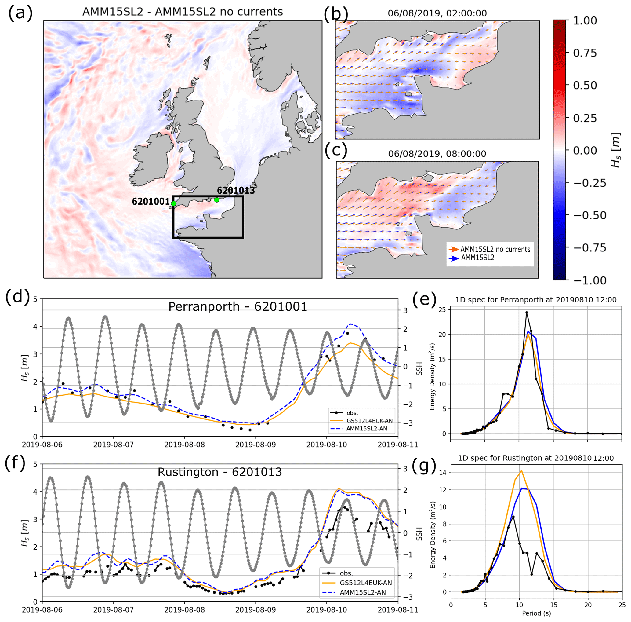
Figure 10Effects of currents in significant wave height (Hs). (a) Mean difference over two tidal cycles (25 h) between AMM15SL2 and GS512L4EUK for Hs across UK waters. (b, c) Snapshots of Hs difference over the English Channel (see panel for an enlarged reference) during ebb (b) and flood tide (c) conditions with vectors for wave direction. (d, f) Time series of sea surface height (SSH) and Hs and (e, g) 1D spectra in Perranporth (6201001) and Rustington (6201013) directional Waveriders during a storm event in August 2019. Wave buoy locations are presented in panel (a).
5.5 Impact of resolution on wave growth
Increased resolution has been demonstrated to play an important role in the model skill score. However, the advantages of using a higher spatial resolution in AMM15SL2 do not always show in the overall skill of Hs. It is known that model simulations can show significant sensitivity to the spatial resolution and source term model set-up. All configurations in the Met Office wave forecast system include the same source term tuning parameters (refer to the Supplement), as this has been found to be suitable in previous system versions. To test the sensitivity of spatial resolution, we run a number of WW3 idealised numerical experiments with variable resolution. The domain has an extent of 1000 km × 500 km that is discretised with regular grids of 10, 5 and 2.5 km resolution (experiments 10kmRes, 5kmRes and 2.5kmRes, respectively). All resolutions are then explored for deep-water (flat bathymetry of 1000 m depth) and shallow-water (flat bathymetry of 40 m deep) conditions. The model is forced for 48 h by a constant wind speed ranging from 10 to 30 m s−1. All simulations include the same source term configuration and tuning terms.
Dimensionless fetch-limited growth () curves as a function of dimensionless fetch () for the different idealised experiments are presented in Fig. 11. For reference, the theoretical wave growth relationships derived from observations by Young and Verhagen (YV96; Young and Verhagen, 1996) are also included. The difference in wave growth between resolutions is greater for shorter fetches and lower winds. High-resolution grids (i.e. 2.5kmRes) generate higher waves compared to the YV96 relationship for both deep (Fig. 11a, c, e) and shallow (Fig. 11b, d, f) water. This behaviour for short fetches is consistent for all wind speeds with higher resolution, resulting in larger growth rates. In all cases, differences between resolutions become smaller as the wind speed increases. Idealised experiments suggest that the increased resolution in AMM15SL2-AN might lead to faster wave growth and subsequently to larger Hs for mid- to high-energy wind conditions in fetch-limited areas. Accordingly, model–observation results show that, for modal conditions, although both models tend to slightly overestimate Hs, AMM15SL2-AN presents a weaker skill reproducing Hs in certain locations. Conversely, extremes, although generally underestimated (not shown), tend to be better replicated by AMM15SL2-AN, mainly in fetch-limited locations (e.g. at Start Bay; Fig. 8a, b). The implication is that, to obtain a similar behaviour in all model configurations, the next generation of Met Office modelling systems should include a modified parameterisation that is domain-dependent, as the current source term set-up is more optimised for GS512L4EUK configuration and modal conditions.
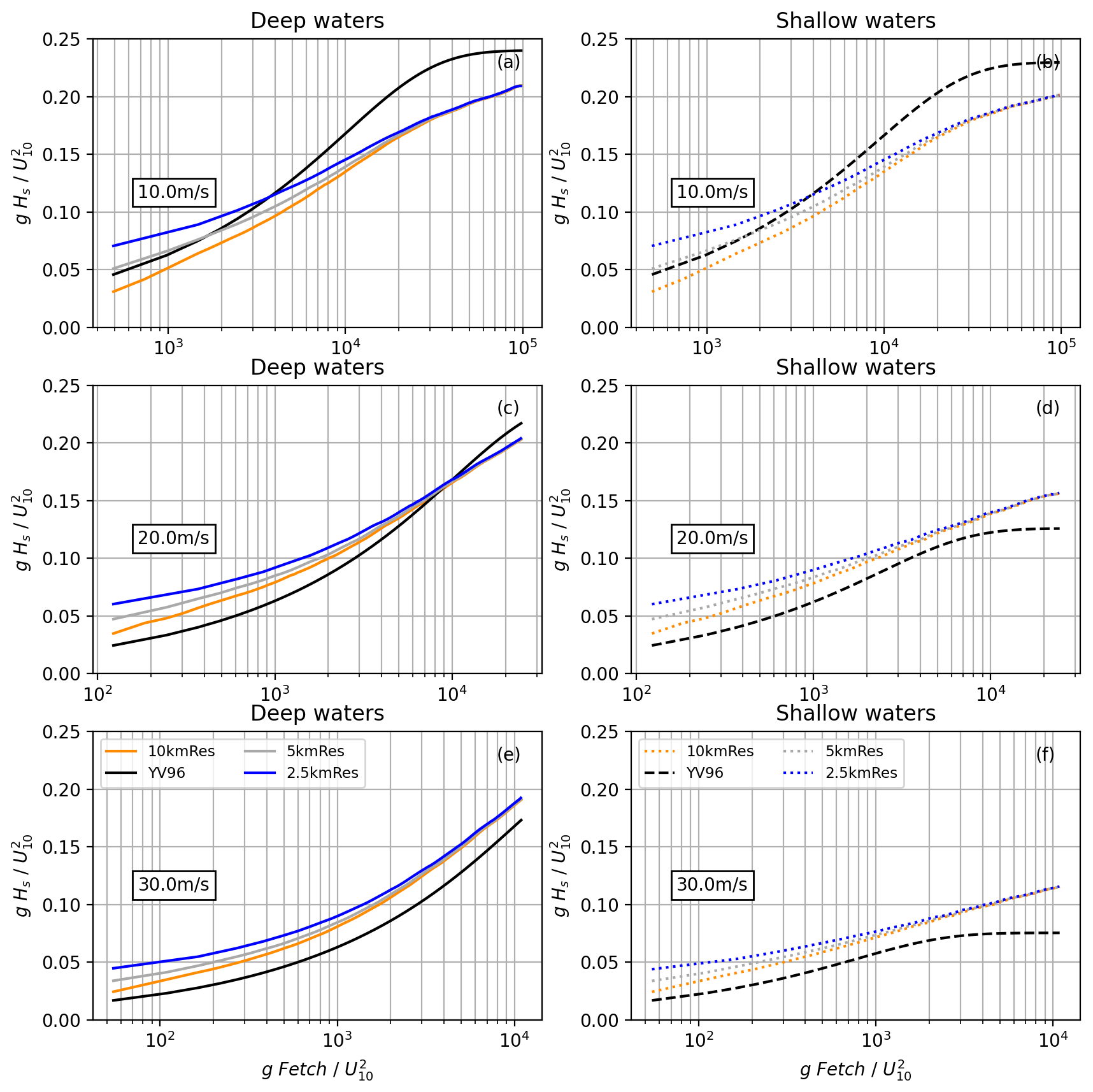
Figure 11Dimensionless wave growth curves for different model grid resolutions (10, 5 and 2.5 km) as a function of dimensionless fetch. Fetch-limited growth curves are computed for (a, c, e) deep water and (b, d, f) shallow water (40 m depth) for constant winds of 10, 20 and 30 m s−1. The theoretical curve of Young and Verhagen (1996) is presented (YV96). Results for the different configurations correspond to 48 h model runs.
We have presented a comprehensive evaluation of the baseline configurations of the Met Office operational forecasting system, namely the global GS512L4EUK and the regional AMM15SL2. Both configurations show good performance when compared to different observation datasets, and this skill is retained for all lead times in the forecast. We have illustrated the benefits of the SMC grid that allows the resolution of the propagation in open waters at lower resolution and incorporation of the effect of complex bathymetry and coastline as waves approach to shore. We paid particular attention to studying two relevant aspects that describe the benefits provided by AMM15SL2, namely the impact of incorporating currents and the implications of higher resolutions in wave growth.
Recent studies have demonstrated positive impacts on significant wave height prediction when surface ocean currents are accounted for (e.g. Palmer and Saulter, 2016; Ardhuin et al., 2017; Echevarria et al., 2021; Valiente et al., 2021b). AMM15SL2-based configuration includes wind and sea surface currents as forcing conditions. Accurate representation of the wave–current interactions across the NW shelf–UK waters domain is essential, as ocean–wave coupling improves accuracy of the ocean surface dynamics by 4 % (Bruciaferri et al., 2021). Additionally, it is clear that the presence of currents can modify the distribution of the wind waves on the shelf with >15 % impact during modal conditions (e.g. Ardhuin et al., 2017; Valiente et al., 2021b; Alday et al., 2022). Although relative changes in T02 metrics and wave Dir show an overall significant improvement (>25 % in RMSD and 10 % in bias), the quantitative assessment to demonstrate the improvement of the forecast skill in the significant wave height diagnostic by AMM15SL2 with respect to GS512L4EUK proves difficult in some instances. The lag between the model and observations present in some in situ locations due to the tidal modulation (i.e. larger spread on the observation–model differences and a possible double-penalty effect; Crocker et al., 2020), together with an excessive bulk energy imparted to the ocean surface waves in AMM15SL2 configuration (consequence of the numerical choice), led sometimes to poorer metrics than when no currents and higher resolution are used (i.e. GS512L4EUK).
Discretisation and numerical schemes (e.g. Roland and Ardhuin, 2014), together with forcing accuracy and the choice of the parameterisation for wave growth and dissipation (e.g. Ardhuin et al., 2010; Zieger et al., 2015) are among the main factors affecting the accuracy of a spectral model (e.g. Alday et al., 2022). In our evaluation, we show that resolution and the choice of the numerical tuning significantly influence the model accuracy. Furthermore, model skill improvement representing modal/extreme conditions can be optimised, but this often leads to the degradation of part of the distribution of the wave field. The Met Office configuration changes from ST4 source term defaults included a combination of a reduction in the sheltering for short waves (TAUWSHELTER term) and a bulk adjustment to the wind field through a decrease in the maximum value allowed for wind–wave coupling (BETAMAX term), leading to an increase in model accuracy in reproducing the tail of the distribution that subsequently led to some degradation in those sectors where the model was already overestimating.
The latest developments and performance of the current Met Office operational wave system have been presented. Imminent system developments will incorporate the following.
-
Use of sea point wind forcing in the SMC grid, improving the wind transfer between atmosphere and ocean. The change in the pre-processing of the wind forcing conditions task will include sea point winds (i.e. SMC grid cells) instead of the current pre-processing step, where winds are interpolated to the underlaying grid resolution (25 km for GS512L4EUK and 3 km for AMM15SL2), in which 10 km NWP Met Office wind resolution for the global domain is upscaled. This development will help to correct some of the wave model behaviour in areas of the globe where an improvement in wind speed and direction due to the higher-resolution interpolation is likely to be an important factor.
-
Optimisation of the models is in line with the model resolution. Idealised scenarios showed resolution-dependent wave growth, indicating that it is important to optimise the source term parameterisation for the different spatial resolutions. Model–observation errors observed in AMM15SL2 for modal conditions are expected to be reduced after the retuning of the regional model to better match observations across the coastal UK waters, as currently this is more optimised to better capture extremes and for the global model.
-
SMC multi-grid. Implementation of a multi-grid approach for the global domain will allow for improved scaling and hybrid parallelisation (component and domain decomposition) in the hybrid Message Passing Interface (MPI)–OpenMP mode (Li, 2022).
Future systems will include the waves as a system component of a more comprehensive atmosphere–wave–ocean–land–ice system. This implies, in most cases, a need to develop more integrated systems, where the different physical components (i.e. atmosphere, ocean, ice and waves) are coupled (e.g. Lewis et al., 2019; Bruciaferri et al., 2021; Valiente et al., 2021a; Castillo et al., 2022). In recent years, the Met Office has put significant effort into developing fully coupled models, and although an operational AMM15 ocean–wave coupled system has been deployed, more complex atmosphere–wave–ocean coupled models are currently in a pre-operational research phase. The GS512L4EUK wave model described in this paper is in the process of being implemented in a global research atmosphere–ocean–ice–wave coupled configuration; however, it will need time before it becomes operational. For the case of the operational AMM15 ocean–wave coupled with data assimilation, this is currently run once a day, providing a 5 d forecast. This is still computationally expensive, with increased resource demands, over the wave-only operational model, with currents as forcing, that delivers data four times a day. Met Office internal testing demonstrates that a coupled simulation leads to a 10 % increase in the running time per model with respect to their standalone version; i.e. if an ocean model needs n nodes to run, and a wave model needs m nodes, then the ocean–wave coupled simulation of the two will need n+m nodes, with an increase of 20 % in the running time. While studies continue toward a fully coupled prediction system with atmosphere, ocean, land, ice and wave components, the maintenance and development of each of the model components is crucial in NWP.
The current Met Office operational wave model forecasting system was described and system performance illustrated by the global (GS512L4EUK) and the NW shelf–UK waters (AMM15SL2) baseline configurations presented. The model–observation correlation is beyond 0.94–0.96 in all areas of analysis, with standard deviations of differences that correspond to maximum values of 13 %–25 % of the observed mean bulk wave diagnostics, demonstrating the quality and accuracy of the Met Office wave forecast capability. This showcases the benefits of the SMC grid, a Met Office development, which provides computational efficiency, while retaining good performance when compared to observations at both global scale and near the shore.
Met Office configurations are optimised to accurately predict modal conditions, with a tendency to slightly overestimate. We show that tidal currents produce a residual signal that presents a more realistic-looking wave time series but can affect the final accuracy of the model. That is, areas in which the tidal currents increase (decrease) the significant wave height led to some degradation (improvement) of this parameter by AMM15SL2.
The inclusion of wave–current effects and the higher resolution for depths <40 m in AMM15SL2, together with a better representation of the local features (e.g. headlands; highly spatially variable bathymetry), result in an incremental improvement in the representation of the wave field, mainly in the frequency and directional domain. The prediction of the wave direction near the coast is improved within a range of ±30 ∘ and the mean period shows >20 % reduction in the RMSD with respect to GS512L4EUK. This is also a consequence of the increase in the wind forcing resolution (10 km), as winds in AMM15SL2 are not presently upscaled in the pre-processing routine performed for GS512L4EUK (i.e. 10 km resolution winds are interpolated to a 25 km regular grid).
We demonstrate that the resolution and the choice of the numerical tuning significantly influences the model accuracy. Evidence of resolution-dependent differences in wave growth was observed, leading to slightly overestimated significant wave heights when replicating coastal mid-range conditions by AMM15SL2. This is better suited to replicating the extremes, particularly for regions with short and mid fetches such as the North Sea.
The improved skill of AMM15SL2, together with a better prediction of mean up-crossing period and wave direction, have large implications for the prediction of waves in short fetched areas and coastal locations. This provides benefits for both off-shore infrastructures, such as wind power or oil platforms, and for coastal applications like beach safety, risk to flooding and overtopping and shoreline evolution in general. It is also recognised that, despite the good skill of AMM15SL2 in replicating inshore waves, the model utility in coastal zones that are largely sheltered and/or with strong shallower water bathymetric variability should be treated with caution, as there are important nonlinear effects that are not included in any of the baseline configurations.
-
Obtaining WAVEWATCH III®. The version of WAVEWATCH III® used operationally at the Met Office is publicly available via the Met Office's Trusted Institutional Fork of the NOAA WW3 GitHub repository (https://github.com/ukmo-waves/WW3/tree/ukmo_ps45-1.hotfixes, last access: 1 February 2023, and can also be found via https://doi.org/10.5281/zenodo.7874843, WW3DG, 2023). The WAVEWATCH III® code base is distributed by NOAA under an open-source-style licence (https://polar.ncep.noaa.gov/waves/wavewatch/wavewatch.shtml, NOAA, 2021a). Interested readers wishing to access the code are requested to register to obtain a licence (see https://polar.ncep.noaa.gov/waves/wavewatch/license.shtml; NOAA, 2021b). Refer to the Supplement for more details.
-
Obtaining configuration files. The basics of the system configuration, including the grid, modules and tuning parameter files are publicly available (https://doi.org/10.5281/zenodo.7148687; Valiente et al., 2022).
The length, resolution and spatial coverage of the data generated in running the trials described in this paper require a large storage facility. The complete or partial data will be available upon request to the corresponding author. Data used for the model evaluation and analysis in this paper in the form of model observation match-up netCDF files are available via https://doi.org/10.5281/zenodo.7019826 (Valiente, 2022).
Datasets for model evaluation include different sources. SHPSYN in situ observations are accessible via the Global Telecommunication System but are also publicly available at http://www.marineinsitu.eu/dashboard/ (Copernicus Marine Environment Monitoring Service in Situ Thematic Assembly Centre, 2022). WAVENET in situ data can be obtained from the National Network of Regional Coastal Monitoring Programmes and CEFAS Wavenet and should be available following registration at http://www.channelcoast.org/ (NNRCMP, 2022) and https://www.cefas.co.uk/cefas-data-hub/wavenet/ (Cefas, 2022). JCOMM-WFVS observations are obtainable from the Met Office, as it is part of the World Meteorological Organisation – International Oceanographic Commission (WMO-IOC) Joint Commission On Marine Meteorology's operational Wave Forecast Verification Scheme. MA_SUP03 satellite altimeter data are available for public download and can be obtained following registration via FTP at ftp://ftp.ifremer.fr/ifremer/cersat/products/swath/altimeters/waves/data (last access: 8 November 2022) MA_SUP03 satellite altimeter data (https://doi.org/10.5285/3ef6a5a66e9947d39b356251909dc12b, Dodet et al., 2022; Piolle et al., 2020).
Additional information on the data acquisition of the different observational datasets used in this paper is included in the Supplement.
The supplement related to this article is available online at: https://doi.org/10.5194/gmd-16-2515-2023-supplement.
NGV conceptualised the experiments, set up and ran the baseline trials, conducted the formal analysis and wind and wave verification, in addition to the data curation, wrote the original draft and prepared the figures/visualisation. AS and BG helped with conceptualisation, validation of resources and review and editing of draft. CB and JGL contributed to the model description and provided a figure for the SMC visualisation. CP performed AMM15 current validation. CB, AS, JGL, NGV and TP contributed to the development of the wave operational system. All of the co-authors contributed to the editing of the final version of the paper.
The contact author has declared that none of the authors has any competing interests.
Publisher's note: Copernicus Publications remains neutral with regard to jurisdictional claims in published maps and institutional affiliations.
We thank the editor and the two anonymous reviewers for their comments and suggestions – these have significantly improved the paper. Simulations were conducted on the Cray HPC at the Met Office, UK.
This paper was edited by Julia Hargreaves and reviewed by two anonymous referees.
Alday, M., Ardhuin, F., Dodet, G., and Accensi, M.: Accuracy of numerical wave model results: application to the Atlantic coasts of Europe, Ocean Sci., 18, 1665–1689, https://doi.org/10.5194/os-18-1665-2022, 2022.
Ardhuin, F., Rogers, E., Babanin, A., Filipot, J.-F., Magne, R., Roland, A., Queffelou, P., Lefevre, J. M., Aouf, L., Babanin, A., and Collard, F.: Semi-empirical dissipation source functions for wind-wave models: part I, definition, calibration and validation at global scales, J. Phys. Oceanogr., 40, 1917–1941, 2010.
Ardhuin, F., Roland, A., Dumas, F., Bennis, A.-C., Sentchev, A., Forget, P., Wolf, J., Girard, F., Osuna, P., and Benoit, M.: Numerical Wave Modeling in Conditions with Strong Currents: Dissipation, Refraction, and Relative Wind, J. Phys. Oceanogr., 42, 2101–2120, https://doi.org/10.1175/JPO-D-11-0220.1, 2012.
Ardhuin, F., Gille, S. T., Menemenlis, D., Rocha, C. B., Rascle, N., Chapron, B., Gula, J., and Molemaker, J.: Small-scale open ocean currents have large effects on wind wave heights, J. Geophys. Res.-Oceans, 122, 4500–4517, https://doi.org/10.1002/2016JC012413, 2017.
Battjes, J. A. and Janssen, P.: Energy loss and set-up due to breaking of random waves, Coast. Eng., 1, 32, https://doi.org/10.9753/icce.v16.32, 1978.
Bidlot, J., Wittmann, P., Fauchon, M., Chen, H., Lefèvre, J. M., Bruns, T., Greensdale, T., Ardhuin, F., Kohno, N., and Park, S.: Inter-comparison of operational wave forecasting systems, in: 10th International Workshop on Wave Hindcasting and Forecasting and Coastal Hazard Symposium, North Shore, Oahu, Hawaii, 11–16 November 2007, 1–22, http://www.waveworkshop.org/10thWaves/Papers/paper_10th_workshop_Bidlot_at_al.pdf (last access: 27 April 2023), 2007.
Booij, N. and Holthuijsen, L. H.: Propagation of ocean waves in discrete spectral wave models, J. Comput. Phys., 68, 307–326, https://doi.org/10.1016/0021-9991(87)90060-X, 1987.
Brown, A., Milton, S., Cullen, M., Golding, B., Mitchell, J., and Shelly, A.: Unified modeling and prediction of weather and climate: A 25-year journey, B. Am. Meteorol. Soc., 93, 1865–1877, https://doi.org/10.1175/BAMS-D-12-00018.1, 2012.
Bruciaferri, D., Tonani, M., Lewis, H. W., Siddorn, J. R., Saulter, A., Castillo Sanchez, J. M., Valiente, N. G., Conley, D., Sykes, P., Ascione, I., and McConnell, N.: The Impact of Ocean-Wave Coupling on the Upper Ocean Circulation During Storm Events, J. Geophys. Res.-Oceans, 126, e2021JC017343, https://doi.org/10.1029/2021JC017343, 2021.
Bunney, C. and Saulter, A.: An ensemble forecast system for prediction of Atlantic-UK wind waves, Ocean Model., 96, 103–116, https://doi.org/10.1016/j.ocemod.2015.07.005, 2015.
Castillo, J. M., Lewis, H. W., Mishra, A., Mitra, A., Polton, J., Brereton, A., Saulter, A., Arnold, A., Berthou, S., Clark, D., Crook, J., Das, A., Edwards, J., Feng, X., Gupta, A., Joseph, S., Klingaman, N., Momin, I., Pequignet, C., Sanchez, C., Saxby, J., and Valdivieso da Costa, M.: The Regional Coupled Suite (RCS-IND1): application of a flexible regional coupled modelling framework to the Indian region at kilometre scale, Geosci. Model Dev., 15, 4193–4223, https://doi.org/10.5194/gmd-15-4193-2022, 2022.
Cavaleri, L. and Rizzoli, P. M.: Wind Wave Prediction in Shallow Water: Theory and Applications, J. Geophys. Res., 86, 10961–10973, https://doi.org/10.1029/JC086iC11p10961, 1981.
Cefas: Homepage, https://www.cefas.co.uk/cefas-data-hub/wavenet/, last access: 8 November 2022.
Copernicus Marine Environment Monitoring Service in Situ Thematic Assembly Centre: Homepage, http://www.marineinsitu.eu/dashboard/, last access: 8 November 2022.
Crocker, R., Maksymczuk, J., Mittermaier, M., Tonani, M., and Pequignet, C.: An approach to the verification of high-resolution ocean models using spatial methods, Ocean Sci., 16, 831–845, https://doi.org/10.5194/os-16-831-2020, 2020.
Dodet, G., Piolle, J.-F., Quilfen, Y., Abdalla, S., Accensi, M., Ardhuin, F., Ash, E., Bidlot, J.-R., Gommenginger, C., Marechal, G., Passaro, M., Quartly, G., Stopa, J., Timmermans, B., Young, I., Cipollini, P., and Donlon, C.: The Sea State CCI dataset v1: towards a sea state climate data record based on satellite observations, Earth Syst. Sci. Data, 12, 1929–1951, https://doi.org/10.5194/essd-12-1929-2020, 2020.
Echevarria, E. R., Hemer, M. A., and Holbrook, N. J.: Global implications of surface current modulation of the wind-wave field, Ocean Model., 161, 101792, https://doi.org/10.1016/j.ocemod.2021.101792, 2021.
Good, S., Fiedler, E., Mao, C., Martin, M. J., Maycock, A., Reid, R., Good, S., Fiedler, E., Mao, C., Martin, M. J., Maycock, A., Reid, R., Roberts-Jones, J., Searle, T., Waters, J., While, J., and Worsfold, M.: The current configuration of the OSTIA system for operational production of foundation sea surface temperature and ice concentration analyses, Remote Sensing, 12, 720, https://doi.org/10.3390/rs12040720, 2020.
Graham, J. A., O'Dea, E., Holt, J., Polton, J., Hewitt, H. T., Furner, R., Guihou, K., Brereton, A., Arnold, A., Wakelin, S., Castillo Sanchez, J. M., and Mayorga Adame, C. G.: AMM15: a new high-resolution NEMO configuration for operational simulation of the European north-west shelf, Geosci. Model Dev., 11, 681–696, https://doi.org/10.5194/gmd-11-681-2018, 2018.
Hasselmann, K., Barnett, T. P., Bouws, E., Carlson, H., Cartwright, D. E., Enke, K., Ewing, J. A., Gienapp, H., Hasselmann, D. E., Kruseman, P., Meerburg, A., Muller, P., Olsbers, D. J., Richter, K., Sell, W., and Walden, H.: Measurements of wind-wave growth and swell decay during the joint North Sea wave project (JONSWAP), https://repository.tudelft.nl/islandora/object/uuid:f204e188-13b9-49d8-a6dc-4fb7c20562fc?collection=research (last access: 8 October 2022), 1973.
Hasselmann, S., Hasselmann, K., Allender, J. H., and Barnett, T. P.: Computations and Parameterizations of the Nonlinear Energy Transfer in a Gravity-Wave Specturm. Part II: Parameterizations of the Nonlinear Energy Transfer for Application in Wave Models, J. Phys. Oceanogr., 15, 1378–1391, https://doi.org/10.1175/1520-0485(1985)015<1378:CAPOTN>2.0.CO;2, 1985.
Hersbach, H. and Bidlot, J.-R.: The relevance of ocean surface current in the ECMWF analysis and forecast system, in: ECMWF Workshop on Ocean-atmosphere interactions, Reading, UK, 10–12 November 2008, 61–73, https://www.ecmwf.int/sites/default/files/elibrary/2009/9866-relevance-ocean-surface-current-ecmwf-analysis-and-forecast-system.pdf (last access: 8 October 2022), 2008.
Janssen, P.: The Interaction of Ocean Waves and Wind, Cambridge University Press, 386 pp., https://doi.org/10.1017/cbo9780511525018, 2004.
King, R. R., While, J., Martin, M. J., Lea, D. J., Lemieux-Dudon, B., Waters, J., and O'Dea, E.: Improving the initialisation of the Met Office operational shelf-seas model, Ocean Model., 130, 1–14, https://doi.org/10.1016/j.ocemod.2018.07.004, 2018.
Lewis, H. W., Castillo Sanchez, J. M., Arnold, A., Fallmann, J., Saulter, A., Graham, J., Bush, M., Siddorn, J., Palmer, T., Lock, A., Edwards, J., Bricheno, L., Martínez-de la Torre, A., and Clark, J.: The UKC3 regional coupled environmental prediction system, Geosci. Model Dev., 12, 2357–2400, https://doi.org/10.5194/gmd-12-2357-2019, 2019.
Li, J. G.: Upstream nonoscillatory advection schemes, Mon. Weather Rev., 136, 4709–4729, https://doi.org/10.1175/2008MWR2451.1, 2008.
Li, J. G.: Global transport on a spherical multiple-cell grid, Mon. Weather Rev., 139, 1536–1555, https://doi.org/10.1175/2010MWR3196.1, 2011.
Li, J. G.: Propagation of ocean surface waves on a spherical multiple-cell grid, J. Comput. Phys., 231, 8262–8277, https://doi.org/10.1016/j.jcp.2012.08.007, 2012.
Li, J.-G.: Hybrid multi-grid parallelisation of WAVEWATCH III model on spherical multiple-cell grids, J. Parallel Distr. Com., 167, 187–198, https://doi.org/10.1016/j.jpdc.2022.05.002, 2022.
Li, J. G. and Saulter, A.: Unified global and regional wave model on a multi-resolution grid, Ocean Dynam., 64, 1657–1670, https://doi.org/10.1007/s10236-014-0774-x, 2014.
Madec, G. and the NEMO team: NEMO ocean engine, Note du Pôle de modélisation, No. 27, Institut Pierre-Simon Laplace (IPSL), France, ISSN 1288-1619, 2016.
National Network of Regional Coastal Monitoring Programmes (NNRCMP): Homepage, http://www.channelcoast.org/, last access: 8 November 2022.
NOAA: WAVEWATCH III® Production Hindcast, Multigrid: Feb 2005 to May 2019, https://polar.ncep.noaa.gov/waves/hindcasts/prod-multi_1.php (last access: 8 November 2022), 2020.
NOAA: WAVEWATCH III® model main page, NOAA [code], https://polar.ncep.noaa.gov/waves/wavewatch/wavewatch.shtml (last access: 4 May 2023), 2021a.
NOAA, WAVEWATCH III® Source Code Request, NOAA [code], https://polar.ncep.noaa.gov/waves/wavewatch/license.shtml (last access: 4 May 2023), 2021b.
Palmer, T. and Saulter, A.: Evaluating the effects of ocean current fields on a UK regional wave model, Met Office Research Technical Report No: 612, https://library.metoffice.gov.uk/Portal/Default/en-GB/DownloadImageFile.ashx?objectId=407&ownerType=0&ownerId=212801 (last access: 26 November 2022), 2016.
Phillips, O. M.: Spectral and statistical properties of the equilibrium range in wind-generated gravity waves, J. Fluid Mech., 156, 505–531, https://doi.org/10.1017/S0022112085002221, 1985.
Piollé, J.-F., Dodet, G., and Quilfen, Y.: ESA Sea State Climate Change Initiative (Sea_State_cci) : Global remote sensing daily merged multi-mission along-track significant wave height, L3 product, version 1.1., Centre for Environmental Data Analysis [data set], https://doi.org/10.5285/3ef6a5a66e9947d39b356251909dc12b, 2020.
Roland, A. and Ardhuin, F.: On the developments of spectral wave models: Numerics and parameterizations for the coastal ocean, Ocean Dynam., 64, 833–846, https://doi.org/10.1007/s10236-014-0711-z, 2014.
Saulter, A.: North West European Shelf Production Centre – Quality Information Document, 1–60, https://catalogue.marine.copernicus.eu/documents/QUID/CMEMS-NWS-QUID-004-014.pdf (last access: 26 November 2022), 2020.
Saulter, A., Bunney, C., and Li, J.: Application of a refined grid global model for operational wave forecasting, Forecasting Met Office Research Technical Report No: 614, 46, https://doi.org/10.13140/RG.2.2.22242.17600, 2016.
Saulter, A., Bunney, C., Li, J.-G., and Palmer, T.: Process and resolution impacts on UK coastal wave predictions from operational global-regional wave models, in: The 1st International Workshop on Waves, Storm Surges and Coastal Hazards incorporating the 15th international workshop on wave hindcasting and forecasting, Liverpool, United Kingdom, September 2017, http://www.waveworkshop.org/15thWaves/Papers/K1_WHF_SaulterEtAl_UKCoastalWave_20170913.pdf (last access: 8 November 2022), 2017.
Saulter, A. N., Bunney, C., King, R. R., and Waters, J.: An Application of NEMOVAR for Regional Wave Model Data Assimilation, Front. Mar. Sci., 7, 579834, https://doi.org/10.3389/fmars.2020.579834, 2020.
Siddorn, J. R., Good, S. A., Harris, C. M., Lewis, H. W., Maksymczuk, J., Martin, M. J., and Saulter, A.: Research priorities in support of ocean monitoring and forecasting at the Met Office, Ocean Sci., 12, 217–231, https://doi.org/10.5194/os-12-217-2016, 2016.
Tolman, H. L.: User manual and system documentation of WAVEWATCH III® version 4.18, http://polar.ncep.noaa.gov/waves/wavewatch/manual.v4.18.pdf (last access: 8 December 2022), 2014.
Tonani, M., Sykes, P., King, R. R., McConnell, N., Péquignet, A.-C., O'Dea, E., Graham, J. A., Polton, J., and Siddorn, J.: The impact of a new high-resolution ocean model on the Met Office North-West European Shelf forecasting system, Ocean Sci., 15, 1133–1158, https://doi.org/10.5194/os-15-1133-2019, 2019.
Tonani, M., Bruciaferri, D., Pequignet, C., King, R., Sykes, P., McConnell, N., Siddorn, J., Saulter, A., and Ascione, I.: North West European Shelf Production Centre – Quality Information Document, NORTHWESTSHELF_ANALYSIS_FORECAST_PHYS_004_013, Issue: 1.5, 1–52, https://catalogue.marine.copernicus.eu/documents/QUID/CMEMS-NWS-QUID-004-013.pdf (last access: 26 November 2022), 2022.
Valckle, S., Craig, T., and Coquart, L.: OASIS3 MCT User Guide OASIS3-MCT_3.0, Cerfacs, Technical Report TR/CMGC/15/38, https://www.cerfacs.fr/oa4web/oasis3-mct_3.0/oasis3mct_UserGuide.pdf (last access: 4 May 2023), 2015.
Valiente, N. G.: Supporting data – The Met Office operational wave forecasting system: the evolution of the Regional and Global models, Zenodo [data set], https://doi.org/10.5281/zenodo.7019826, 2022.
Valiente, N. G., Saulter, A., Edwards, J. M., Lewis, H. W., Sanchez, J. M. C., Bruciaferri, D., Bunney, C., and Siddorn, J.: The impact of wave model source terms and coupling strategies to rapidly developing waves across the north-west european shelf during extreme events, Journal of Marine Science and Engineering, 9, 403, https://doi.org/10.3390/jmse9040403, 2021a.
Valiente, N. G., Saulter, A., and Lewis, H. W.: The effect of different levels of coupling in surface wind waves along the NWS during extreme events, Met Office Forecasting Research Technical Report No:642, https://digital.nmla.metoffice.gov.uk/ (last access: 26 November 2022), 2021b.
Valiente, N. G., Saulter, A., Bunney, C., and Gomez, B.: Configurations files – The Met Office operational wave forecasting system: the evolution of the Regional and Global models, Zenodo [code], https://doi.org/10.5281/zenodo.7148687, 2022.
Walters, D., Baran, A. J., Boutle, I., Brooks, M., Earnshaw, P., Edwards, J., Furtado, K., Hill, P., Lock, A., Manners, J., Morcrette, C., Mulcahy, J., Sanchez, C., Smith, C., Stratton, R., Tennant, W., Tomassini, L., Van Weverberg, K., Vosper, S., Willett, M., Browse, J., Bushell, A., Carslaw, K., Dalvi, M., Essery, R., Gedney, N., Hardiman, S., Johnson, B., Johnson, C., Jones, A., Jones, C., Mann, G., Milton, S., Rumbold, H., Sellar, A., Ujiie, M., Whitall, M., Williams, K., and Zerroukat, M.: The Met Office Unified Model Global Atmosphere 7.0/7.1 and JULES Global Land 7.0 configurations, Geosci. Model Dev., 12, 1909–1963, https://doi.org/10.5194/gmd-12-1909-2019, 2019.
Waters, J., Lea, D. J., Martin, M. J., Mirouze, I., Weaver, A., and While, J.: Implementing a variational data assimilation system in an operational 1/4degree global ocean model, Q. J. Roy. Meteor. Soc., 141, 333–349, https://doi.org/10.1002/qj.2388, 2015.
Williams, K. D., Copsey, D., Blockley, E. W., Bodas-Salcedo, A., Calvert, D., Comer, R., Davis, P., Graham, T., Hewitt, H. T., Hill, R., Hyder, P., Ineson, S., Johns, T. C., Keen, A. B., Lee, R. W., Megann, A., Milton, S. F., Rae, J. G. L., Roberts, M. J., Scaife, A. A., Schiemann, R., Storkey, D., thorpe, L., Watterson, I. G., Walters, D. N., West, A., Wood, R. A., Woollings, T., and Xavier, P. K.: The Met Office Global Coupled Model 3.0 and 3.1 (GC3.0 and GC3.1) Configurations, J. Adv. Model. Earth Sy., 10, 357–380, https://doi.org/10.1002/2017MS001115, 2018.
Young, I. R. and Verhagen, L. A.: The growth of fetch limited waves in water of finite depth. Part 1. Total energy and peak frequency, Coast. Eng., 29, 47–78, 1996.
WAVEWATCH III Development Group (WW3DG): User manual and system documentation of WAVEWATCH III® version 6.07. Tech. Note 333, NOAA/NWS/NCEP/MMAB, College Park, MD, USA, 465 pp. + Appendices, https://raw.githubusercontent.com/wiki/NOAA-EMC/WW3/files/manual.pdf (last access: 1 November 2022), 2019.
WW3 Development Group (WW3DG): ukmo-waves/WW3:ukmo_ps45-1.1, Zenodo [code], https://doi.org/10.5281/zenodo.7874843, 2023.
Zieger, S., Babanin, A. V., Rogers, W. E., and Young, I. R.: Observation-based source terms in the third-generation wave model WAVEWATCH, Ocean Model., 96, 2–25, https://doi.org/10.1016/j.ocemod.2015.07.014, 2015.
- Abstract
- Introduction
- The Met Office operational wave models
- Observations and metrics for model accuracy
- Forecast performance
- Model evaluation
- Discussion and ongoing development
- Conclusions
- Code availability
- Data availability
- Author contributions
- Competing interests
- Disclaimer
- Acknowledgements
- Review statement
- References
- Supplement