the Creative Commons Attribution 4.0 License.
the Creative Commons Attribution 4.0 License.
 | 05 May 2023
LISFLOOD-FP 8.1: new GPU-accelerated solvers for faster fluvial/pluvial flood simulations
Mohammad Kazem Sharifian
Georges Kesserwani
Alovya Ahmed Chowdhury
Jeffrey Neal
Paul Bates
The local inertial two-dimensional (2D) flow model on LISFLOOD-FP, the so-called ACCeleration (ACC) uniform grid solver, has been widely used to support fast, computationally efficient fluvial/pluvial flood simulations. This paper describes new releases, on LISFLOOD-FP 8.1, for parallelised flood simulations on the graphical processing units (GPUs) to boost efficiency of the existing parallelised ACC solver on the central processing units (CPUs) and enhance it further by enabling a new non-uniform grid version. The non-uniform solver generates its grid using the multiresolution analysis (MRA) of the multiwavelets (MWs) to a Galerkin polynomial projection of the digital elevation model (DEM). This sensibly coarsens the resolutions where the local topographic details are below an error threshold ε and allows classes of land use to be properly adapted. Both the grid generator and the adapted ACC solver on the non-uniform grid are implemented in a GPU new codebase, using the indexing of Z-order curves alongside a parallel tree traversal approach. The efficiency performance of the GPU parallelised uniform and non-uniform grid solvers is assessed for five case studies, where the accuracy of the latter is explored for and 10−3 in terms of how close it can reproduce the prediction of the former. On the GPU, the uniform ACC solver is found to be 2–28 times faster than the CPU predecessor with increased number of elements on the grid, and the non-uniform solver can further increase the speed up to 320 times with increased reduction in the grid's elements and decreased variability in the resolution. LISFLOOD-FP 8.1, therefore, allows faster flood inundation modelling to be performed at both urban and catchment scales. It is openly available under the GPL v3 license, with additional documentation at https://www.seamlesswave.com/LISFLOOD8.0 (last access: 12 March 2023).
- Article
(25907 KB) - Full-text XML
- BibTeX
- EndNote


LISFLOOD-FP is a raster-based open-source hydrodynamic modelling framework that has been applied in many fields of earth sciences, including morphodynamic modelling (Coulthard et al., 2013; Ziliani et al., 2020), urban drainage modelling (Wu et al., 2018; Yang et al., 2022), population mapping (Zhu et al., 2020), coastal flooding (Hirai and Yasuda, 2018; Seenath, 2018), uncertainty quantification (Liu and Merwade, 2018; Beevers et al., 2020; Jafarzadegan et al., 2021; Karamouz and Mahani, 2021; Yin et al., 2022; Zeng et al., 2022) and coupled hydrological–hydraulic modelling (Siqueira et al., 2018; Towner et al., 2019; Hoch et al., 2019; Rajib et al., 2020; Makungu and Hughes, 2021; Nandi and Reddy, 2022). It has undergone extensive developments and testing since its conception (e.g. Bates and De Roo, 2000; Hunter et al., 2005; Bates et al., 2010; Sosa et al., 2020; Shustikova et al., 2020; Zhao et al., 2020), becoming a state-of-the-art tool for flood modelling applications at urban, catchment, regional and continental scales (e.g. Amarnath et al., 2015; Chaabani et al., 2018; Zhu et al., 2019; O'Loughlin et al., 2020; Zare et al., 2021; Bessar et al., 2021; Choné et al., 2021; Asinya and Alam, 2021; Zhao et al., 2021).
LISFLOOD-FP includes a variety of numerical schemes to solve the two-dimensional (2D) shallow water equations, which can be written as
where Eq. (1) is the mass conservation equation, and Eqs. (2)–(3) are the momentum conservation equations. In these equations, h [L] represents the water depth, and qx=hu and qy=hv [L2 T−1] are the discharge per unit width in the x and y orthogonal directions, respectively, expressed involving the velocity components u and v [L T−1]; r [L T−1] is the prescribed rainfall rate, g [L T−12] is the gravitational acceleration, z [L] is the two-dimensional topographic elevation and nM is Manning's coefficient [L]. Along with the finite volume and discontinuous Galerkin schemes that solve the full form of Eqs. (1)–(3) (Shaw et al., 2021), two simplified schemes are also available in LISFLOOD-FP: a diffusive wave scheme, that neglects both acceleration and advection terms, and a local inertial scheme, that neglects the advection term but includes the acceleration term (hence referred to as the ACC solver). The extra complexity of including the acceleration term in the ACC solver pays off with larger and more stable time steps than the diffusive wave solver (Hunter et al., 2006, 2008; Bates et al., 2010; Wang et al., 2011). Compared to the finite volume and Galerkin schemes, the ACC solver is faster to run since it also does not deploy an approximate Riemann solver (Shaw et al., 2021): it uses a hybrid finite difference–volume numerical scheme over a compact computational stencil in a staggered approach, which evaluates continuous discharges at the interfaces between adjacent grid elements, to achieve an element-wise update of averaged water levels (Bates et al., 2010). Consequently, the ACC solver has been favoured to run fast and sufficiently accurate simulations for fluvial floods from rivers and/or for rainfall-driven pluvial floods, featured with gradually propagating 2D flows over rough areas with Manning parameters higher than 0.03 m (Neal et al., 2012b; de Almeida and Bates, 2013). It has received further developments to sustain its utility and speed for such applications: for instance, the ACC solver has been enabled with a subgrid channel model to integrate the flow from river channels with any width below that of the grid resolution (Neal et al., 2012a) and its efficiency maximised on the central processing unit (CPU) with shared-memory parallelisation with an optimised treatment of wet–dry zones (Neal et al., 2018). Still, the ACC solver can be further sustained with alternative speed-up measures to enable faster and more efficient simulations across a wide range of spatial scales and grid resolutions (Guo et al., 2021).
One useful speed-up measure is the capability of running the ACC solver on a non-uniform grid with sensibly coarsened resolutions in the smooth portions of the digital elevation model (DEM) alongside proper distribution of different classes of land use such as, for example, different classes of Manning parameters. Such a non-uniform grid can be generated while introducing one error threshold parameter, ε: by reshaping the DEM into a planar Galerkin projection and then applying the multiresolution analysis (MRA) of multiwavelets (MWs) (Kesserwani et al., 2019; Kesserwani and Sharifian, 2020; Özgen-Xian et al., 2020). The scheme of the ACC solver can readily be adapted to the non-uniform grid, hereafter referred to as the non-uniform grid solver. Another useful speed-up measure is to further exploit the parallelism of the graphical processing unit (GPU) architecture. This can be achieved without any complication for the uniform solver due to the uniformity of the indexing system, using nested grid-stride loops in the existing GPU codebase developed in Shaw et al. (2021). However, an ad hoc codebase must be designed to make the non-uniform grid solver run efficiently on the GPU, namely, to accommodate the irregular grid resolution layout featured in the MRA process of the grid generator and handle data reindexing, access, distribution and update on the non-uniform grid.
This paper describes the design and integration of a non-uniform grid solver on LISFLOOD-FP 8.1 that runs on the GPU. The portability of the uniform solver to the existing GPU codebase (Shaw et al., 2021) is straightforward and will therefore not be presented. In Sect. 2, the non-uniform grid solver is described, with a focus on (i) the grid generator that sensibly coarsens local DEM resolutions, (ii) the adaptation of the ACC scheme to conserve fluxes across non-uniformly sized elements and (iii) the ad hoc codebase to efficiently implement both the grid generator and the adapted scheme on the GPU. In Sect. 3, the accuracy of the non-uniform solver is assessed for five realistic flooding case studies for selected ε values, considering the level of closeness of its predictions to those of the uniform solver. The ratio of runtimes is used to evaluate the speed-up gain from the GPU version of the uniform solver with respect to the CPU version and of the non-uniform solver with respect to the uniform solver on the GPU. In Sect. 4, conclusions are drawn on the potential utility of the GPU-accelerated local inertial solvers. The codes of these solvers are openly available (https://doi.org/10.5281/zenodo.6912932, LISFLOOD-FP developers, 2022) for non-commercial use under the GPLv3.0 licence, with a user guide available at https://www.seamlesswave.com/LISFLOOD8.0 (last access: 28 April 2023).
LISFLOOD-FP 8.1 includes a non-uniform grid solver that runs on the GPU architecture. The solver is made of two components: the grid generator that applies the MRA of MWs to a planar Galerkin projection of DEM data to sensibly coarsen resolutions and accordingly adapt classes of land use parameters (Sect. 2.1) and the adapted ACC scheme on the generated grid to aggregate the discharges across non-uniformly sized elements of the grid (Sect. 2.2). Both the grid generator and the adapted ACC scheme are packed in a new codebase to efficiently implement the non-uniform grid solver on the GPU (Sect. 2.3).
2.1 Non-uniform grid generator with spatially varying distribution of friction
Given a 2D rectangular domain spanned by a raster-formatted DEM at resolution R, with px × py pixels (px and py being the number of pixels in the x and y directions, respectively), a maximum refinement level, L, is deduced such that 2L≥px and 2L≥py. Then, a hierarchy of grids of decreasing refinement levels L, L – 1, … , 0 is assumed in a dyadic manner, so that the finest grid has 2L × 2L elements at resolution R, while the coarsest grid has only a single element at resolution 2LR. Figure 1a shows an example of a hierarchy of grids with L=3. The grid generator starts by reshaping the topography data over each element on level L as a planar Galerkin projection (Shaw et al., 2021). The planar data are then recursively produced for the elements on the coarser grids at refinement levels L – 1, L – 2, … , 1, 0 in a process known as “encoding” (Kessewani and Sharifian, 2020). Encoding produces the “details”, representing the encoded difference between the topography data across two subsequent refinement levels, which are generated from the MWs supplements to the planar topographic representation. These details become increasingly significant where there is sharp variation in the topography data but remain small otherwise. The details are then analysed by comparing their magnitude to a user-specified error threshold ε, to only retain a tree-like structure of elements with significant details. Figure 1b shows such a tree-like structure, with “leaf elements” at the end of each branch, specified in colour depending on their refinement level. These leaf elements are then used to assemble a non-uniform grid made of non-overlapping elements at various resolutions, as shown in Fig. 1c. The grid generator can also be used to adapt a spatially varying distribution of land use parameters on the assembled grid. Here, it was used to adapt different classes of Manning's friction parameters by applying the MRA to a raster-formatted Manning's data map that is initially available at resolution level L.
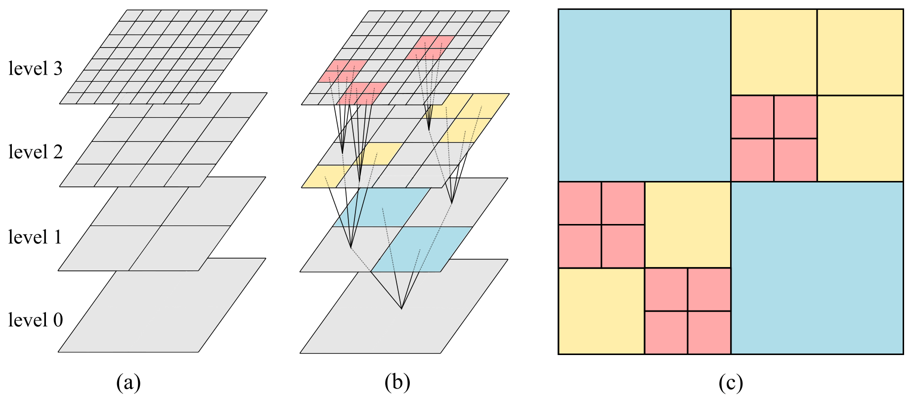
Figure 1Outline of MRA: (a) hierarchy of grids, (b) elements associated with the leaf elements of a tree of significant details and (c) non-uniform grid assembled from these elements.
2.2 Adaptation on the non-uniform grid
The non-uniform grid (e.g. Fig. 1c) includes non-uniformly sized faces as each element can have a coarser neighbour or multiple finer neighbours. To adapt the scheme of the ACC solver to such a non-uniform grid, amendments must be made to aggregate the discharge estimates across non-uniformly sized faces from the side of the elements with finer resolution levels. Figure 2 shows an example of an element at position (i, j) (blue element) that is adjacent to an element of resolution that is one level coarser (yellow element, e3) and two elements of resolution that are two levels finer (red elements, e1 and e2) over its eastern face. For instance, the x-directional discharge, Qx (m3 s−1), across element (i, j) and element e1 is calculated as
where Δx is the size of element (i, j), Δxe1 is the size of element e1, is the discharge per unit width, is water surface elevation at each element and hf (m) is calculated as
After computing the discharges over all other three neighbouring interfaces e1, e2 and e3, the total discharge across the eastern face of the element (i, j) is aggregated as
to be used in mass conservation equation to evolve the water depth as
where , and are discharge estimates at the western, southern and northern faces, respectively, computed in the same manner, and Ai,j is the area of element (i, j). Note that the rainfall source term is treated separately such that, at each time step, the water depth updated by Eq. (7) is subsequently updated with the prescribed rainfall rate r.
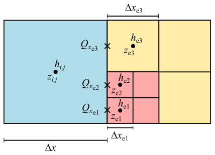
Figure 2Schematic layout of neighbouring elements on a non-uniform grid, where a coarse element (in blue) is adjacent to one- and two-level finer elements (in yellow and red, respectively).
2.3 GPU implementation
The grid generator of the non-uniform solver entails an irregular grid resolution layout to perform the recursive operations of the MRA process and to reindex, access, distribute and update the flow data on the non-uniform grid via the adapted scheme of the ACC solver. In what follows, the GPU implementation of the non-uniform solver is presented with a focus on the parallel handling of the MRA process (Sect. 2.3.1) and preserving neighbourhood relationships on the non-uniform grid (Sect. 2.3.2).
2.3.1 Accommodating MRA process using Z-order curves
To efficiently perform MRA on the GPU, a data structure based on the Z-order curve is deployed, which maps the hierarchy of grids to a single 1D array. A Z-order curve can be created for a 2l × 2l grid by following the so-called Morton codes of the grid elements, which are obtained by bit-interleaving the X and Y indices of each element. Since a Morton code is represented by a 64 bit integer, the two binary representations that are interleaved to produce the Morton code can use up to 32 bit each. Therefore, each binary representation is effectively represented by a 32 bit integer. An example of the creation of a Z-order curve using the Morton codes for a 22 × 22 grid is shown in Fig. 3. As seen in Fig. 3a, X and Y indices are stored in binary form and bit-interleaved, as indicated by the alternating red and black digits. After bit-interleaving the X and Y indices, the resulting Morton codes are converted to their equivalent decimal indices that are then joined in an ascending order to create the Z order, as seen in Fig. 3b.
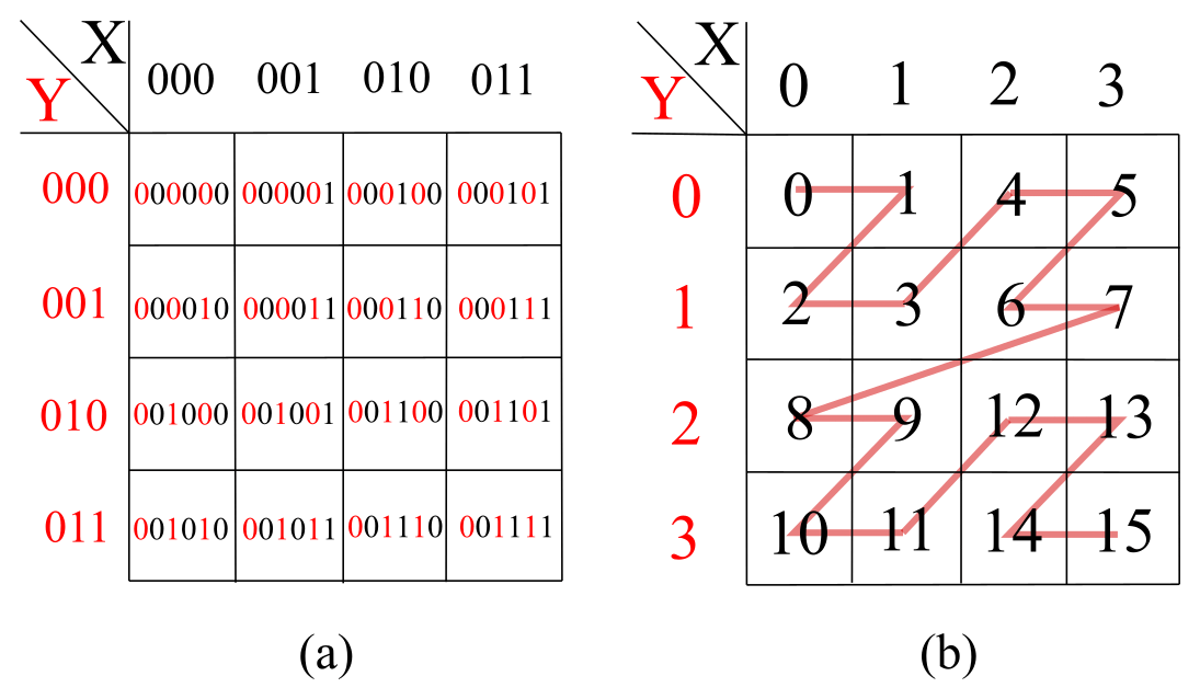
Figure 3Indexing the elements of a grid using a Z-order curve: (a) bit-interleaving the X and Y indices of each element, in binary form, and (b) Morton codes for each element from interleaving, in decimal form.
Z-order curves are created for each grid in the hierarchy of grids to map the hierarchy into a single 1D array residing in GPU memory. Figure 4a shows a hierarchy of grids with L=3 that has been mapped to a 1D array using the Z-order curve. This indexing allows the encoding process to be efficiently performed (e.g. the elements with indexes 9, 10, 11 and 12 that are required to get the details on element 2 all reside in adjacent locations in memory) and the tree of significant details to be formed, as shown in Fig. 4b.
After getting the tree of significant details, a number of GPU threads equal to the number of elements on the finest grid, here 23 × 23=64 threads, are launched. All these threads start at the element with index 0 and climb the branches of the tree until they reach the leaf element and record it, as shown in Fig. 4c. Depending on the resolution level of the leaf elements, some threads might record duplicate indices. These duplicate indices are removed to reduce the number of threads when assembling the non-uniform grid, as shown in Fig. 4d.
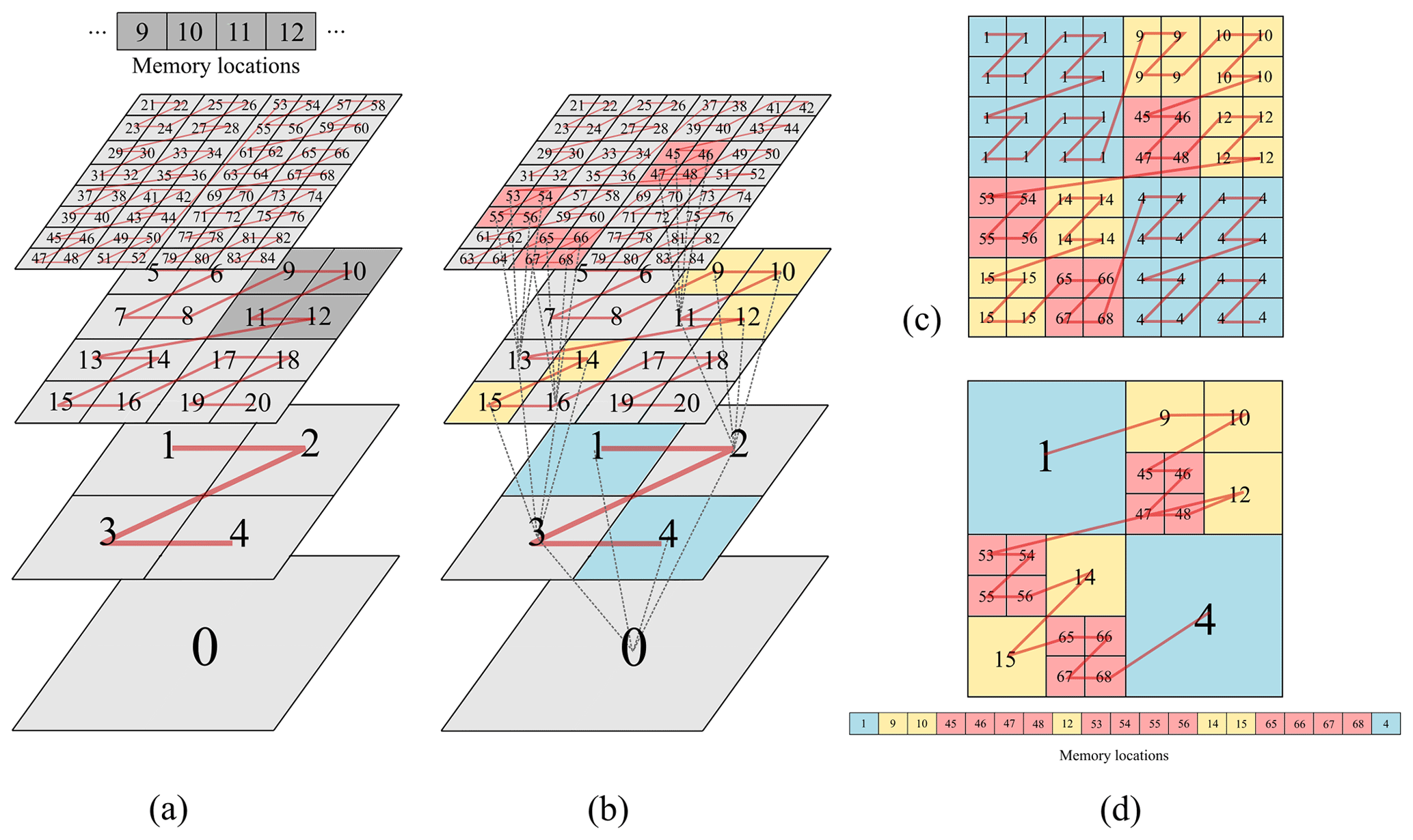
Figure 4(a) Indexing of each grid in the 3D hierarchy of grids using Z-order curves; (b) the tree of significant details indexed using Z-order curves; (c) indices recorded by each GPU thread, including duplicate indices; and (d) the Z-order curve of the final assembled non-uniform grid after removing duplicate indices.
2.3.2 Preserving neighbourhood relationships on the non-uniform grid
The element-wise update using the non-uniform solver's scheme requires aggregating the discharges at each face it shares with the other neighbouring elements. Therefore, each element must find and store neighbour relationships about all of its neighbours to be able to loop over the faces. These relationships can be stored by an equivalent representation of the non-uniform grid projected onto the finest grid, as shown in Fig. 4c. In Fig. 4c, element 1 is located at refinement level l=1 and comprises 16 duplicate indices. It has four neighbours on the northern, eastern, southern and western sides. Considering the array of 16 duplicates, by knowing both current resolution level l and the maximum refinement level L, the Morton codes of two points located at the southwest and northeast of the array can be found. Using these two Morton codes, all the indices at the four sides of element 1 can be identified while removing the duplicate indices to locate and save the actual neighbouring elements.
2.4 Updates to LISFLOOD-FP utilities for running the non-uniform
The non-uniform ACC solver is distributed as a new release for LISFLOOD-FP 8.1 and follows the same standard usage for the other solvers with a few updates to input/output components. In order to use the solver, first, the user needs to reshape the DEM data as planar Galerkin projected data (recall Sect. 2.1). This is achieved using a utility application called generateDG2DEM, which loads the raw DEM raster file and generates three new raster files containing the average (i.e. .dem format) and x-slope and y-slope topography coefficients (i.e. .dem1x and .dem1y format). Configuring a specific simulation using the non-uniform ACC solver requires setting one additional parameter of the error threshold, ε, and extracting the maximum refinement level parameter, L, from the DEM (recall Sect. 2.1). To account for the rainfall, the model follows the so-called rain-on-grid approach (Costabile et al., 2021), which simply imposes the prescribed rainfall data at grid elements. These prescribed rainfall data can be imported from a simple text file (i.e. .rain format) for spatially uniform and temporally varying rains or from a NetCDF file (i.e. .nc format) for spatially and temporally varying rains. By default, the outputs of the new non-uniform ACC solver can be saved as multiresolution grids in VTK file format to enable the use of visualisation tools such as ParaView (https://www.paraview.org/, last access: 28 April 2023) to plot the non-uniform grid and data. Also, the outputs are further converted to raster files to allow benchmarking on uniform grids. Basic checkpoint/restart capabilities are available to resume computations from a previously saved snapshot. Starting with the 8.0 version, LISFLOOD-FP has transitioned to a new CMake-based build system, following the general trend in the open-source software community, which allows hassle-free building/compiling in a cross-platform manner. A step-by-step guide on how to download and install the code, along with instructions on simulating selected case studies using the new non-uniform solver, is given in a series of supplementary videos (Sharifian and Kesserwani, 2022), along with instructions, at https://www.seamlesswave.com/LISFLOOD8.0 (last access: 28 April 2023).
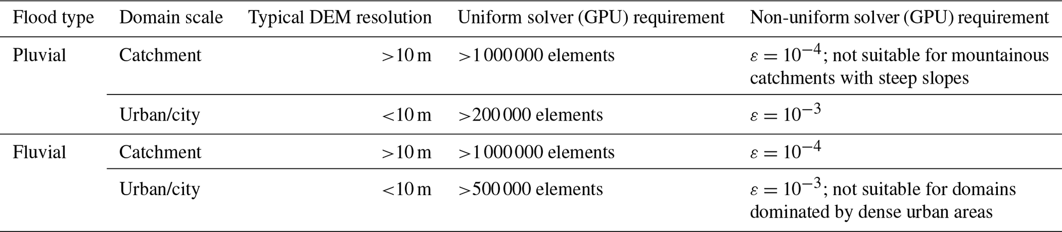
The efficiency of the GPU versions of the uniform and non-uniform grid solvers is assessed by applying them to reproduce realistic fluvial and/or pluvial flooding scenarios. Five case studies are selected and investigated to demonstrate the potential utility of the solvers for both catchment-scale and urban-scale flood simulations. The case studies are described in Table 1, which also includes information on the maximum refinement level, L, used to generate the grid with the non-uniform solver, and on the DEM resolution, R, at which the uniform solver was run. Non-uniform and uniform grid simulations were run on an Nvidia Quadro RTX 2070 SUPER GPU card. The uniform grid simulations were also run for the CPU version reported in Neal et al. (2018), on a 3.8 GHz Intel i7 8700 with 12 CPU threads, which led to identical predictions to those achieved on the GPU version. The closeness of the predictions from the non-uniform simulations to those of the uniform grid simulations depends on the choice for the error threshold, ε. As this choice needs to be such that to preserve an acceptable level of closeness (Kesserwani and Sharifian, 2020), the non-uniform solver simulations were run considering and 10−4. In this sense, the accuracy will hereafter refer to the level of closeness of the non-uniform solver simulations to those achieved by the uniform solver simulations on the finest resolution, R, that can be available on its grid.
Table 1Selected case studies used: to benchmark the accuracy of the non-uniform grid solver against the uniform grid solver, to analyse the speed-up gain from the uniform grid solver on the GPU architecture compared to the CPU architecture and to also analyse the speed-up gain acquired by the non-uniform solver over the GPU version of the uniform grid solver.
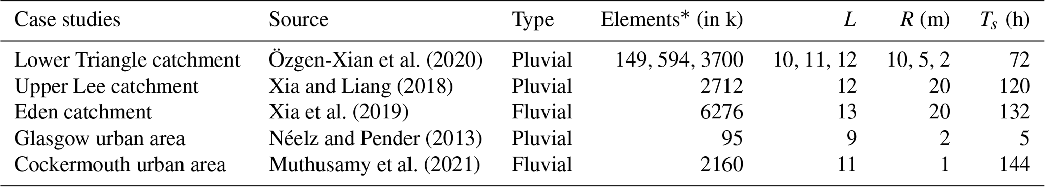
* The number of elements only involves the valid pixels of the DEM, excluding the ones without data.
The maximum flood extent predicted by the non-uniform grid solver is compared to that of the uniform solver using the hit rate (H), false alarm (F) and critical success index (C) (Wing et al., 2017; Hoch and Trigg, 2019). The metric H measures how much the extent predicted by the uniform solver is covered by that predicted by the non-uniform solver (i.e. H=1 indicates full coverage and 0 otherwise). The metric F measures how much of the extent predicted by the non-uniform solver is outside that predicted by the uniform solver (i.e. F=0 indicates that there are no predicted portions by the non-uniform solver that are outside of the extent predicted by the uniform solver, and F=1 indicates that the extent predicted by the former is entirely outside that predicted by the latter). The C metric combines H and F to weigh how much of the sum of both the extents predicted by the uniform and non-uniform solvers is covered by the extent predicted by the non-uniform solver (i.e. C=1 indicates full coverage and 0 otherwise). Interpreting the C metric requires some bespoke judgement for each test case: larger flooded zones in a smaller perimeter of the domain area and represented at increasingly finer resolution are expected to increase the C score as well as the predictive capability of the non-uniform solver (shown later in Sect. 3.4 and 3.5). Nevertheless, as C gets close to 0.8, the predicted flood extent can be deemed to be sufficiently accurate.
The speed-up gain associated with the use of the GPU version of the uniform grid solver, over the CPU version, will be quantified by looking at the ratio of their respective runtimes to complete a simulation. The enhancement in speed-up associated with the use of the non-uniform solver simulation over the uniform solver will be quantified similarly for the GPU versions. The grid predicted by the non-uniform solver entails a reduction in the number of elements with reference to the grid of the uniform solver. Table 2 includes the simulation runtimes and the number of elements consumed by solvers for the selected case studies, from which the speed-up ratios and the reduction in the number of elements will be quantified.
Table 2Simulation runtimes and number of elements on the grid for the uniform solvers (on CPU and GPU architectures) and for the non-uniform solver (GPU architecture) for all the selected case studies.

3.1 Lower Triangle catchment
The case study reproduces a real-world rainfall-runoff event over a mountainous catchment considering three DEM resolutions of 2, 5 and 10 m, which were downscaled from the available 0.5 m DEM resolution in Wainwright and Williams (2017). It aims to assess the accuracy of the non-uniform grid solver with increasingly coarser DEM resolution. The catchment is a sub-catchment of the East River watershed in Colorado, USA, with a surface area of 14.84 km2 featured by high-elevation topography, with steep slopes towards the main river stream located in the middle of the catchment (Fig. 5). The 72 h flood event was induced by a storm that occurred in August 2016, based on the rainfall time series shown in Fig. 5, which was given at 30 min intervals (Wainwright and Williams, 2017). The friction parameter is uniformly set to nM=0.035 m over the domain that was initially dry before a simulation starts. A simulation starts by loading the temporally varying rainfall data, uniformly into all elements on the grid.
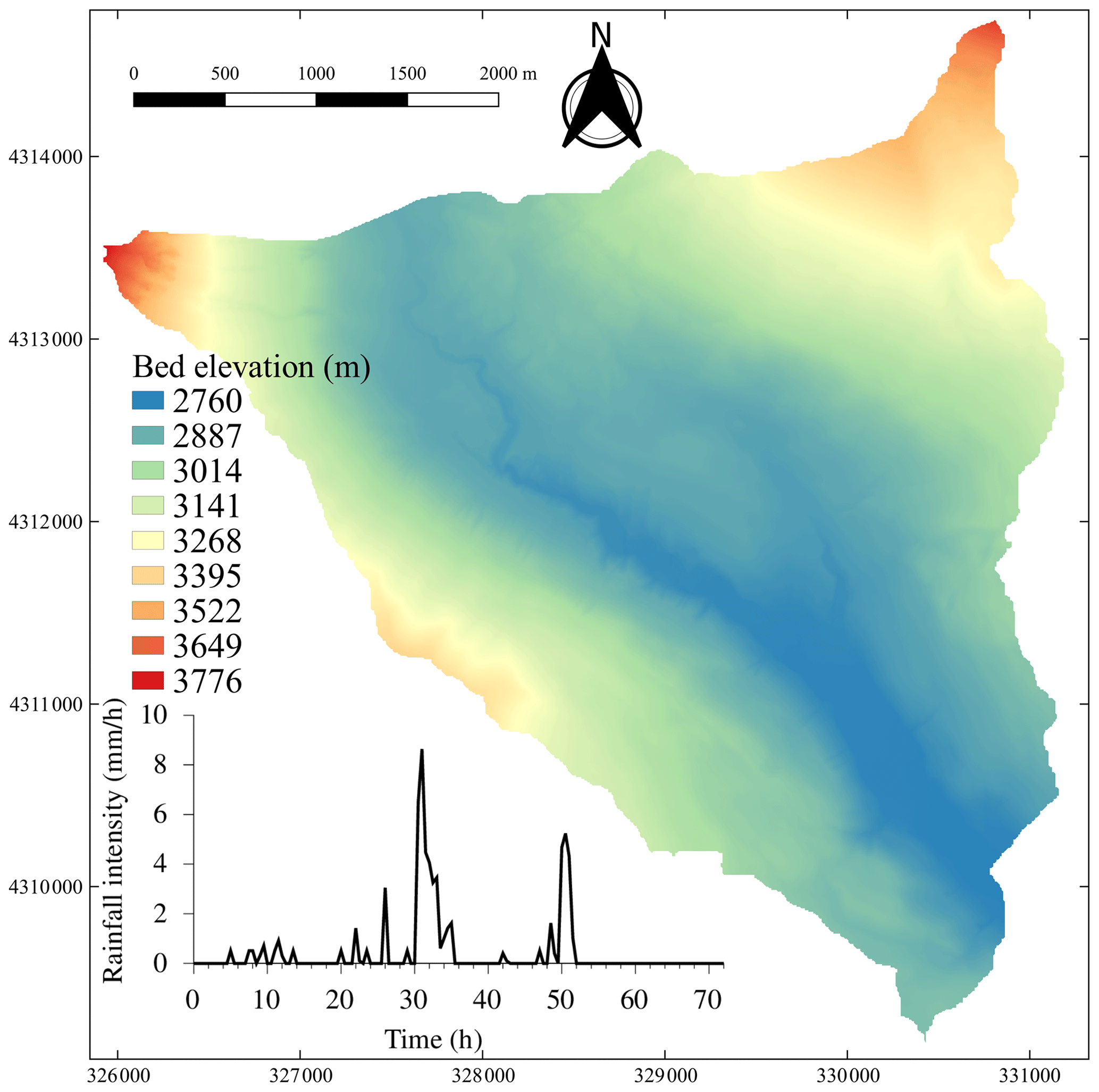
Figure 5Lower Triangle catchment. Topographic map of the domain with a subfigure showing the time series of the spatially uniform rainfall over the catchment.
The ranges of resolutions for the grids predicted by the non-uniform solver are compared in Fig. 6, for the two ε values and the three DEMs considered at 2, 5 and 10 m resolutions. With and the 2 m resolution DEM, the grid predicted shows a dominance for the 8 m resolution as finer resolutions are only reached at the northwest corner with very steep gradients of the topography. This leads to a 93 % reduction in the number of elements, while with the 5 and 10 m resolution DEM, the reduction decreased to 82 % and 66 %, respectively, suggesting that the use of coarser DEM resolutions smoothens the representation of the topographic features. With , the grids predicted by the non-uniform solver show dominance of coarser resolutions ranging between 16 and 32 m, 20 and 40 m, and 40 and 80 m with the use of a 2, 5 and 10 m DEM resolution, respectively. In this case, there are higher than 92 % reductions in the number of elements with the 2, 5 and 10 m resolution DEMs, signalling that is too big.
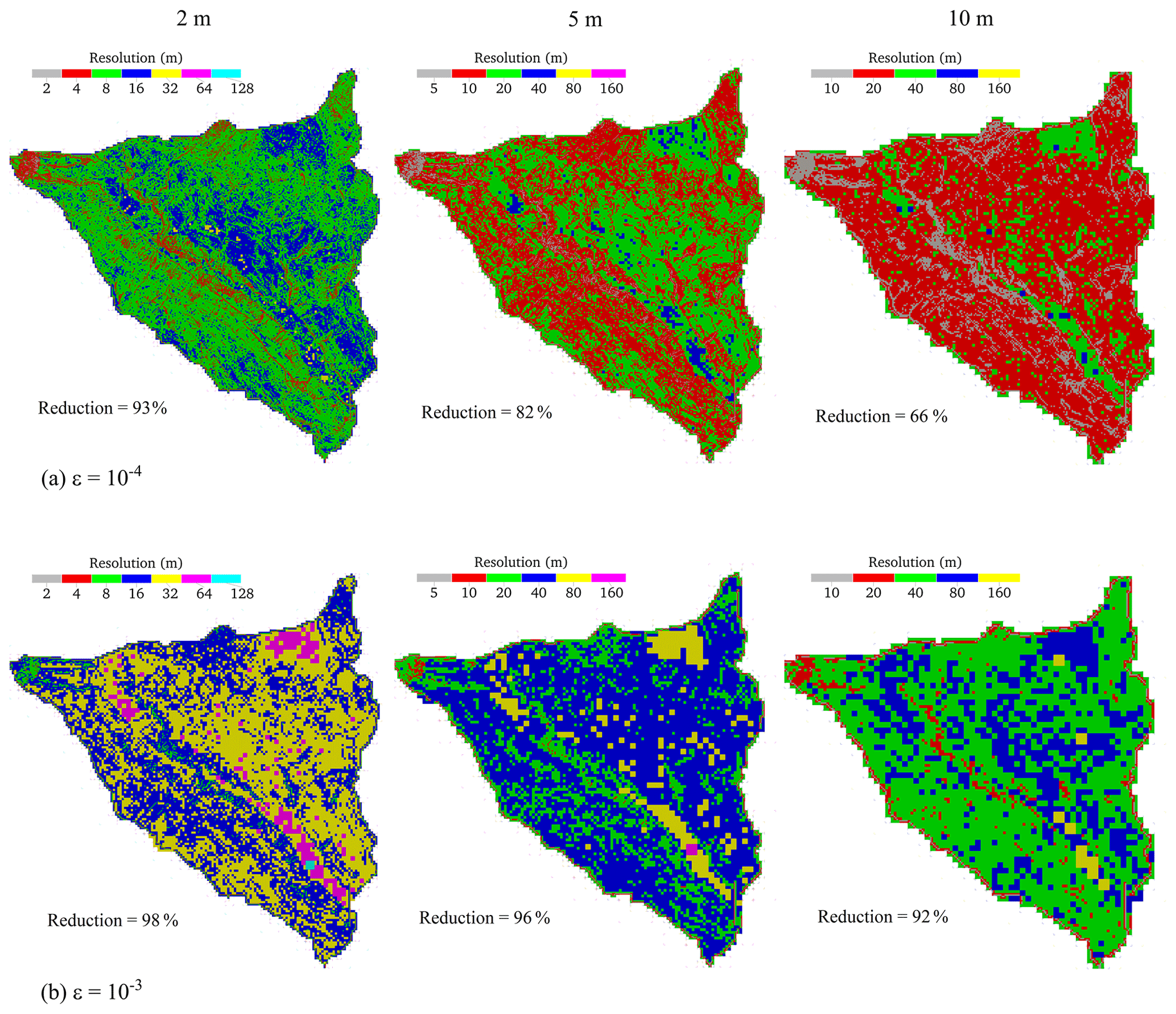
Figure 6Lower Triangle catchment. The resolution maps for the grids generated by the non-uniform solver considering DEM at 2, 5 and 10 m resolutions, using (a) and (b) .
The accuracy of the non-uniform solver predictions for the flood extent is analysed in Fig. 7, which shows the maps of the difference in maximum flood extents for the two ε values. With , at 2 m DEM resolution, the predicted maximum flooded area shows the least agreement with the extent predicted by the uniform grid solver, with a C of 0.56, leading to pronounced underpredictions (red areas, H=0.69) and overpredictions (blue areas, F=0.24) over the tributary streams (Fig. 7a). The relatively poor scores are related to the inherent limitation of the ACC solver in modelling thin, fast-flowing water depths occurring over a very steep terrain from the high-intensity runoff (De Almeida et al., 2012; Sridharan et al., 2021). This is also noted for the coarser 5 and 10 m DEM resolutions, where the overall agreement of the predictions by the non-uniform grid solver becomes close to the uniform grid counterparts, leading to higher C values of 0.61 and 0.67, respectively. Note that improved scores are expected with the mesh coarsening (as discussed in Fig. 6a) since it reduces the steepness of the topographic slopes, which in turn reduces the occurrence of thin and high-velocity flows. The same tendency is observed for the larger , with a more notable loss of accuracy in maximum flood extent predictions that occur due to the higher reductions in the number of elements on the non-uniform grid (Fig. 6b). This loss of accuracy reduces the C values to 0.43, 0.44 and 0.48 for 2, 5 and 10 m DEM resolutions, respectively (Fig. 7b). However, the C values remain close to each other at while remaining lower than 0.5, suggesting that this ε value may be too large for catchment-scale simulations over DEMs at a resolution of 2 m or lower and should, therefore, be avoided (also shown next in Sect. 3.2 and 3.3).
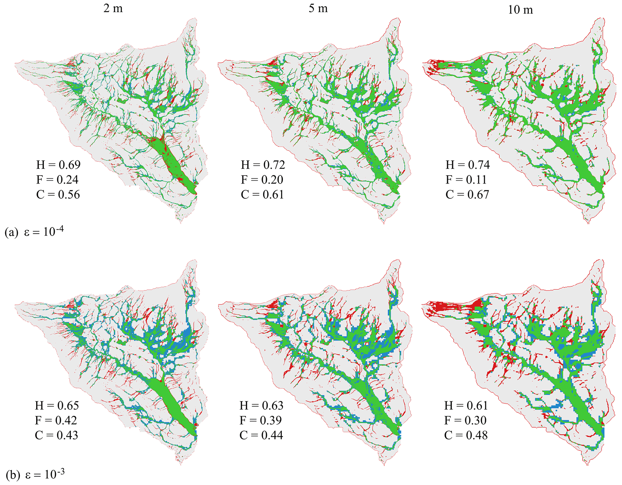
Figure 7Lower Triangle catchment. Difference in the maximum flood extent predicted by the non-uniform grid solver considering DEM resolutions of 2, 5 and 10 m (left to right), using (a) and (b) . Green parts flag flooded areas predicted by both the uniform and the non-uniform grid solvers, blue parts flag an overprediction (i.e. flooded areas only predicted by the non-uniform grid solver), red parts flag an underprediction (i.e. flooded areas only predicted by the uniform grid solver), and white parts flag dry areas predicted by both the uniform and non-uniform solvers. The hit rate (H), false alarm (F) and critical success index (C) values are computed against the flood extents predicted by the uniform grid solver using respective DEMs.
In terms of speed-up, the uniform solver on the GPU architecture is found to be 2.1, 1.65 and 0.9 times faster than the CPU architecture for the 2, 5 and 10 m DEM resolutions, respectively. The decreasing trend in speed-up ratios is expected as the number of elements decreases to less than 600 000 and 200 000, for the 5 and 10 m DEM resolutions, respectively, for which the GPU parallelisation is not too effective in decreasing the runtimes (Shaw et al., 2021). With , the non-uniform solver leads to speed-up ratios of 5.7, 3.0 and 2.4 times over the uniform solver for the 2, 5 and 10 m DEM resolutions, respectively. Such an increasing trend in speed-up with increasingly finer resolutions is expected as there is a higher reduction in the number of elements (Fig. 6a). With , the ratios become 21, 7.6 and 4.7 times, respectively. The significant speed-up achieved for the 2 m DEM resolution comes at the price of deteriorating accuracy (Fig. 7). For the coarser 5 and 10 m DEM resolutions, the speed-ups are less than 2 and 4 times lower, respectively, but there is more deterioration in accuracy.
This case study indicates that the uniform grid solver on GPU architecture is more or less as fast as the CPU architecture when the number of elements is 500 000 or smaller but becomes increasingly faster when the simulation entails a large number of elements. With , the non-uniform solver somewhat preserves a fair accuracy and benefits from increasingly higher speed-ups as its grid entails increasingly higher reduction in the number of elements. With , the solver is unable to preserve an adequate level of accuracy when the resolution is coarse, and the DEM is featured by smooth topographic variations, suggesting to avoid the choice of for such simulations.
3.2 Upper Lee catchment
This case study reproduces a rainfall-flood event in the Upper Lee catchment in north London, UK, which covers an area of 1180 km2, shown in Fig. 8a. The available DEM has a relatively coarse resolution, of 20 m, involving less topographic variations (i.e. less than 200 m), compared to the previous case study (Sect. 3.1). This catchment is also characterised by various classes of land use, shown in Fig. 8b, which have been represented by spatially varying Manning's friction parameter (Table 3) by following commonly recommended values (Chow, 1959). Heavy rainfall was recorded for 120 h between 5 and 11 February 2014, resulting in the flood event. Figure 8c shows the time series of the mean rainfall intensity that includes several rainfall peaks. The initial conditions for the water depth were preprocessed in a raster format to account for the fact that the rivers are initially wet before the simulation starts. The simulation was then solely driven by the spatially and temporarily varying rainfall data. For this case study, an observed discharge hydrograph is available that was recorded at the gauge station located in the river Lee by the outlet of the catchment (Fig. 8a). The accuracy of the non-uniform grid solver in the prediction of the flooding extent will be analysed for a smaller portion of the catchment (i.e. the framed portion in Fig. 8a) that is located upstream of the gauge station from the northeastern side. The impact on flooding extent predictions, over the whole catchment, will be analysed by comparing the solver predictions to the peak flows with reference to the observed hydrograph.
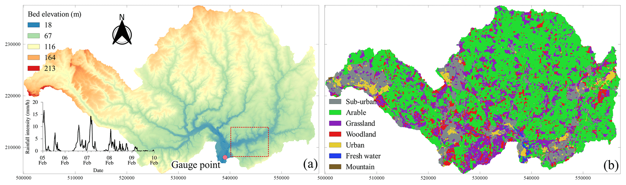
Figure 8Upper Lee catchment. (a) Topographic map of the domain including the position of the gauge point, a subfigure showing the time series of mean (spatially varying) rainfall over the catchment and a framed smaller portion of the domain in which the maximum flood extent is analysed. (b) The land use map of the domain.
Table 3Upper Lee catchment. Values of Manning's friction parameter for different classes of land use.

Figure 9 compares the resolution maps generated from the grid predicted by the non-uniform solver for the two ε values. With , the finest 20 m resolution is seen to cover about 70 % of the catchment area to include the tributaries converging into the main rivers, leading to an overall reduction of 25 % in the number of elements. With the larger , the grid is spanned by the 40 and 80 m resolutions that cover about 90 % of the catchment area. This leads to a higher reduction of 74 %, at the price of entailing overly coarser resolutions to represent the topographic connectivities.
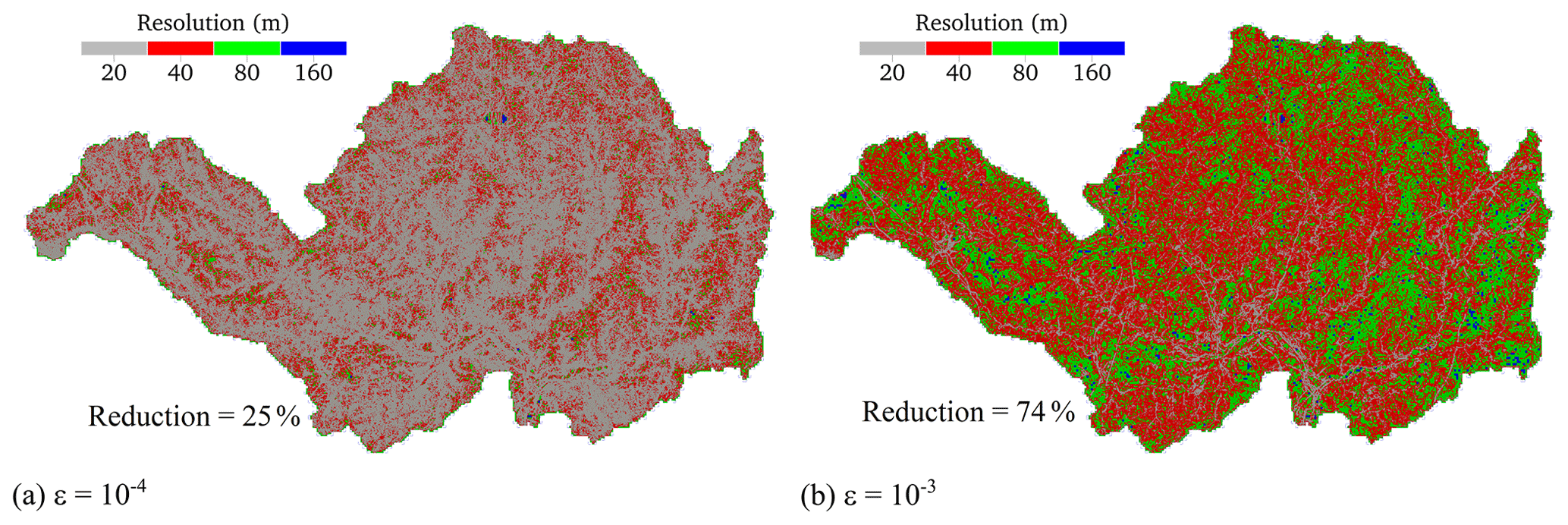
Figure 9Upper Lee catchment. The resolution maps for the grids generated by the non-uniform solver using (a) and (b) .
Figure 10 compares the accuracy of the predictions made by the non-uniform grid solver for the two ε values, in terms of maximum flood extent, for the selected portion of the catchment (Fig. 8a). With (Fig. 10a), the solver accurately predicts the flood extent over the majority of the tributaries and main river streams, with rather high values for H and C metrics, of 0.86 and 0.80, respectively, and a low score for F of 0.07, whereas, with , underpredictions (red-coloured) can be detected mainly around the main river streams and their banks (red areas in Fig. 10b, with lower H, of 0.80), given the relatively coarser resolutions used to represent the topographic connectivity, leading to a reduction in overall accuracy with a lower C, of 0.71.
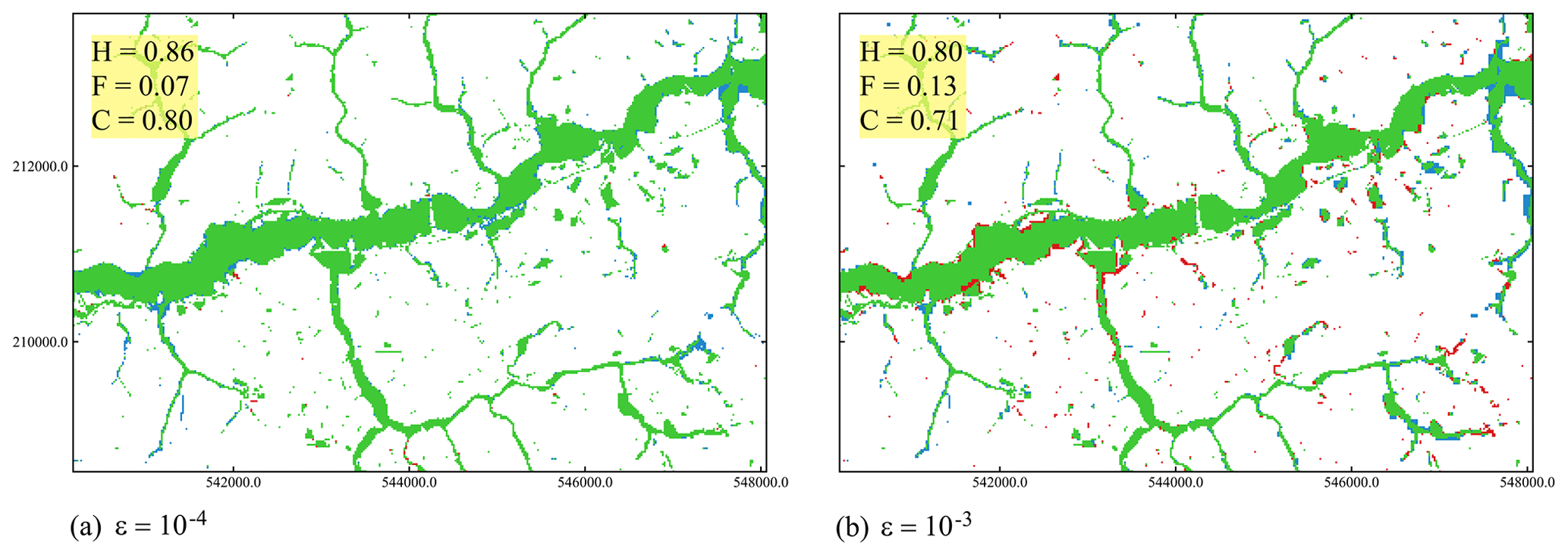
Figure 10Upper Lee catchment. Differences in the maximum flood extent predicted by the non-uniform grid solver using (a) and (b) , over the smaller portion of the domain framed in Fig. 8a. Green parts flag flooded areas predicted by both the uniform and the non-uniform grid solvers, blue parts flag an overprediction (i.e. flooded areas only predicted by the non-uniform grid solver), red parts flag an underprediction (i.e. flooded areas only predicted by the uniform grid solver), and white parts flag dry areas predicted by both the uniform and non-uniform solvers. The hit rate (H), false alarm (F) and critical success index (C) values are computed against the flood extent predicted by the uniform grid solver on 20 m resolution DEM over the whole domain.
The predicted flow discharges at the outlet (post-processed hydrographs) are compared against the observed hydrograph in Fig. 11. None of the simulated hydrographs closely trail the observed hydrograph, including that predicted by the uniform solver. This deficiency can be attributed to uncertainties in the location of the in situ measurements, in the aggregation of the simulated discharges at coarse resolutions that are further magnified by larger numerical diffusions accumulating on the coarser portions of the static non-uniform grid (Kesserwani and Sharifian, 2023) and in the inability of the present Manning's friction law formula to model rain-driven overland flows in the catchment areas with low Reynolds numbers (Taccone et al., 2020), and to the fact that the features of river channel bathymetry are not captured in the 20 m DEM. As shown in Kesserwani and Sharifian (2023), such issues could be alleviated to some extent using dynamic grid adaptivity that deploys a more complex formulation combining the multiresolution analysis (MRA) of the multiwavelets with a second-order discontinuous Galerkin (MWDG2) solver. However, capturing such events more accurately with the present solvers using static grid adaptivity and the ACC solver formulation seems to suggest a need for deploying a DEM resolution that is at most 10 m (Ferraro et al., 2020), which is not available for this case study. Therefore, the predictability of the solvers to the flow discharge at the outlet may here be better evaluated by looking at the extent to which they can reproduce the primary and secondary peaks seen in the observed hydrograph. The uniform solver provides the closest trail to the primary peak, with a deviation of 9 %, and predicts the presence of the secondary peak at the falling limb (occurring between 80 and 90 h). The non-uniform solver, with , although it predicts the rising limb fairly well, underpredicts the primary peak with a larger deviation of 20 % and overlooks the presence of the secondary peak, whereas with , the solver leads to smeared predictions with a larger deviation of 38 %.

Figure 11Upper Lee catchment. Comparison of observed and simulated discharge hydrographs at the catchment outlet (marked in Fig. 8a).
In terms of speed-up, the uniform grid solver on GPU architecture is found to be 21 times faster to run than the CPU architecture. This speed-up is significant, although the number of elements here is 1 million less than in the previous case study for the 2 m resolution (Sect. 3.1). This may be attributed to the less steep variations of the terrain in the Upper Lee catchment, which reduces the chance of occurring very thin water layers flowing downhill slopes and therefore leads to more stability and bigger time steps. With , the non-uniform grid solver offers a marginal speed-up of 1.3 times, which is increased to 3.1 times with the larger ; this is expected as the reduction in the number of elements increases from 25 % to 74 %, respectively (Fig. 9). This retrieves the previous observation (Sect. 3.1), suggesting that the speed-up afforded by the non-uniform grid solver is proportional to the reduction in the number of elements. Though the reduction is much higher with , this value is again deemed impractical for such a coarse resolution catchment-scale simulation; it would in fact allow for more coarsening to a DEM resolution that is already as coarse as 20 m, which impacts accuracy. For such a simulation with the non-uniform solver, choosing is necessary to keep a moderate level of coarsening in favour of accuracy in terms of maximum flood extent prediction while expecting considerable speed-ups over the uniform solver when the reduction in the number of elements exceeds 30 % (shown next in Sect. 3.3). However, predicting hydrographs at critical gauge point(s) located in the catchment seems to signal the need for using finer DEM resolutions with both the present uniform and non-uniform solvers.
3.3 Eden catchment
This case study replicates the rainfall-driven pluvial flooding over the Eden catchment in northwest England, caused by Storm Desmond in December 2015. Figure 12a shows the 2500 km2 catchment, including rivers Irthing, Petteril Caldew and Eden, which form a confluence in the city of Carlisle (Fig. 12b). The storm event was previously stimulated for DEM resolutions ranging from 40 to 5 m, with a variety of uniform grid solvers formulated upon different levels of mathematical and numerical complexity (Xia et al., 2019; Ming et al., 2020; Shaw et al., 2021). In favour of computational efficiency, these studies recommend using the 10 m DEM resolution as it is sufficient to replicate the flood flow dynamics around the urban areas with enough details. Moreover, the uniform ACC solver could capture the required flow features at the coarser 20 m DEM resolution with minor differences (see Fig. 15 in Shaw et al., 2021). For this case study, the 20 m DEM resolution was used to demonstrate the performance of the non-uniform grid solver. This is because the latter could not be run for the 10 m DEM resolution, hampered by the memory costs for the non-uniform grid generation for this large catchment or in other words by the fact that the number of elements cumulated on the grid hierarchy exceeded the capacity of the available GPU cards.
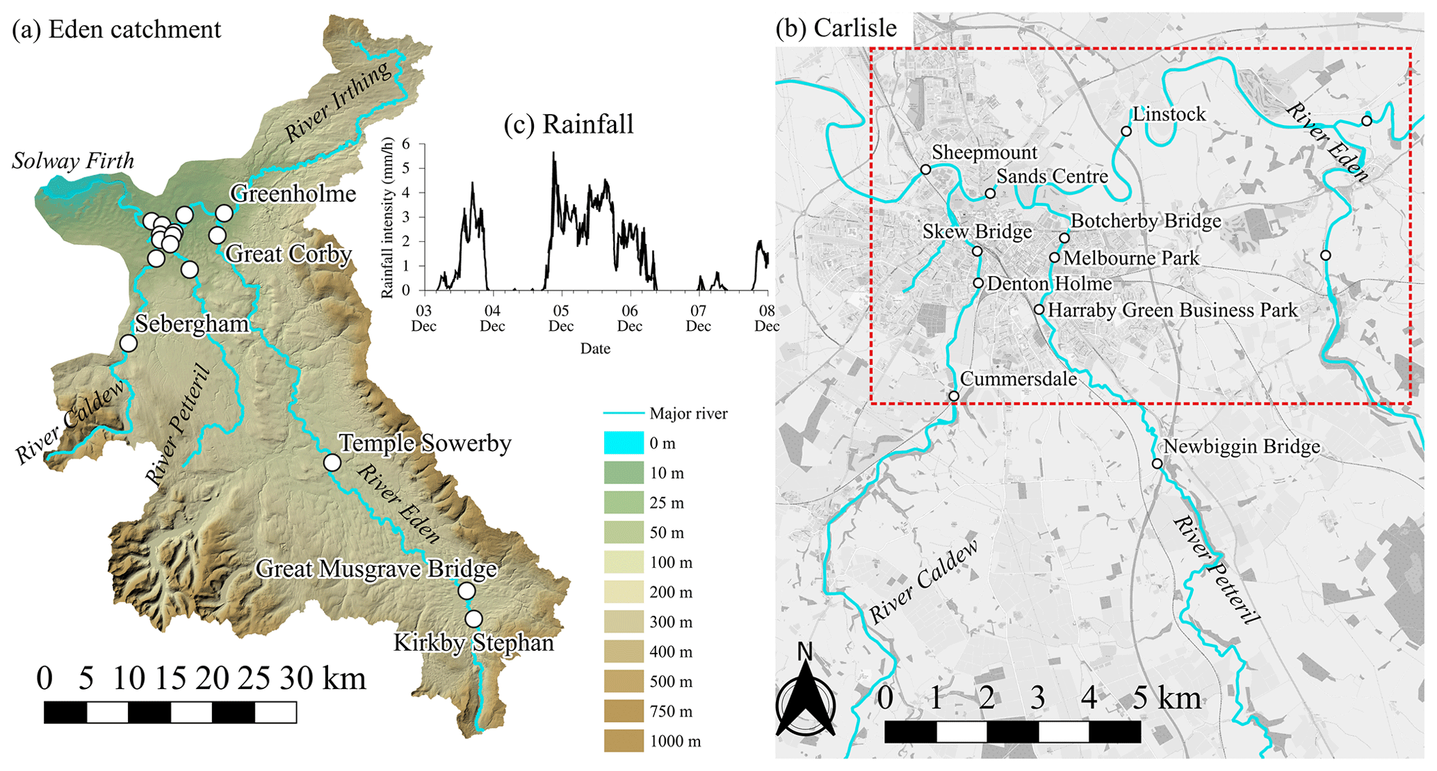
Figure 12Eden catchment. Topographic map of (a) the catchment area covering 2500 km2 and (b) the area over the city of Carlisle at the confluence of rivers Irthing, Petteril, Caldew and Eden. Names and locations of the 16 sampling points are marked, along with the dashed red line framing a smaller portion of the domain where the maximum flood extent was surveyed. Panel (c) shows the time series of mean (spatially varying) rainfall over the catchment. © Google Maps 2021.
A simulation starts at 00:00, 3 December 2015, with a 36 h spin-up from an initially dry domain, and ends at 12:00, 8 December 2015. The spatially and temporally varying rainfall is shown in Fig. 12c, which is provided from radar data at a 1 km spatial resolution and 5 min temporal resolution (Met Office, 2013). The rainfall file, in NetCDF file format, is loaded to start the simulation. The friction parameter is set to nM=0.035 m for river channels and nM=0.075 m for floodplains. The water levels simulated by the uniform and non-uniform grid solvers were recorded in 16 gauge points located in river channels (Fig. 12a and b) to enable comparison with in situ measurements (Environment Agency, 2020). The maximum predicted flood extents were also recorded to enable comparison with a surveyed post-event flood extent in the portion inside the Carlisle area framed in Fig. 12b (McCall, 2016).
Figure 13 shows the range of resolutions predicted on the non-uniform grids for the two ε values. With , it can be seen that the finest 20 m resolution covers more than 50 % of the catchment area, or otherwise the 40 m resolution dominates. The larger leads to 90 % dominance of the 40 and 80 m resolutions over the catchment area, with almost an equal distribution for the 80 m resolution. This reinforces that allows more coarsening than necessary for a DEM resolution as coarse as 20 m (recall Sect. 3.2). The reduction in the number of elements is found to be significantly larger with , to be around 85 %, compared to the 36 % reduction obtained with for which the topographic connectivities in the catchment were represented at the recommended resolutions (Xia et al., 2019; Shaw et al., 2021; Ming et al., 2020).
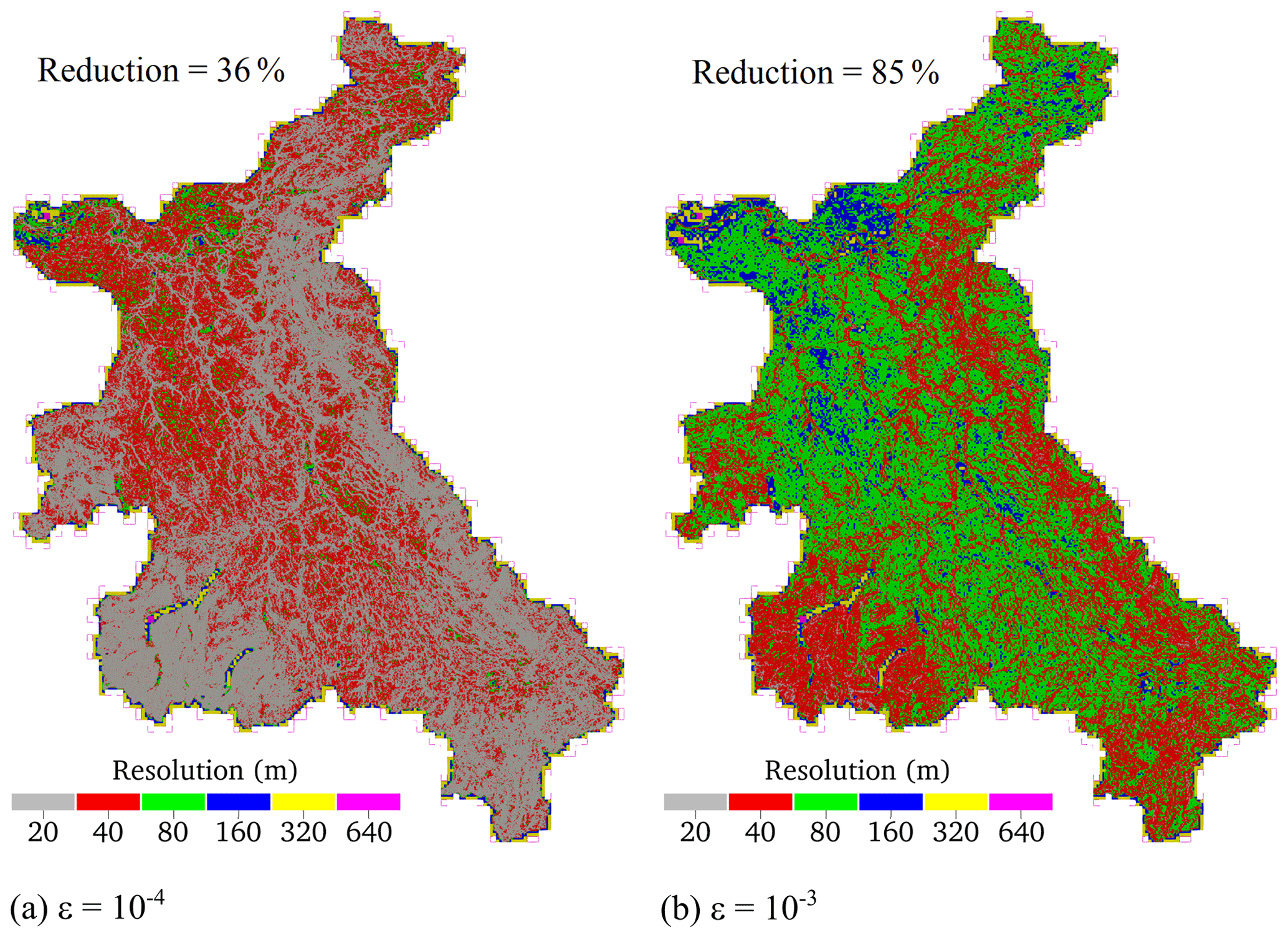
Figure 13Eden catchment. The resolution maps for the grids generated by the non-uniform solver using (a) and (b) .
In Fig. 14, the simulated water level hydrographs extracted from the uniform grid solver (reference hydrographs) are included, showing the best agreement with the observed hydrographs at the 16 gauge points. In contrast to the previous case study, these reference hydrographs do not exhibit short-timescale events, correctly reproducing the observed rising and falling limbs and the peak water levels, namely at the points where the 20 m DEM resolution is sufficient (Shaw et al., 2021). These points include Sheepmount, Sands Centre, Linstock and Great Corby, located in river channels whose widths are 2 to 3 times larger than 20 m (i.e. ranging between 54 and 71 m). The other points are located in river channels whose widths are close to, or less, than 20 m (i.e. ranging between 8 and 33 m), showing a relatively poorer prediction of the observed rising and falling limbs. The underprediction observed at Great Musgrave occurred because of an anomaly from the localised terrain elevation differences between the finest-resolution DEM and riverbed elevation measurements (Xia et al., 2019). The reference hydrographs are next used to evaluate the accuracy of the predictions made by the non-uniform solver.
In terms of accuracy, the non-uniform solver with predicts close water levels to the reference hydrographs predicted by the uniform solver at almost all the gauge points, suggesting that the non-uniform solver at can be a valid alternative to the uniform solver for such a catchment simulation at 20 m DEM resolution. With the large , the non-uniform solver leads to a less accurate trail of the reference hydrographs, such as underpredictions to the peak levels at Sheepmount, Sands Centre, Linstock and Great Corby alongside smearing of the hydrograph profiles at Sebergraham, Greenholm and Botchery Bridge. This loss in accuracy is caused by the poorer representation of the topographic features excluding river streams on a grid dominated by the 80 m resolution (Fig. 13), which confirms the impracticability of using with the non-uniform grid solver for generic catchment-scale simulations dominated by DEM resolutions that are strictly coarser than 20 m.
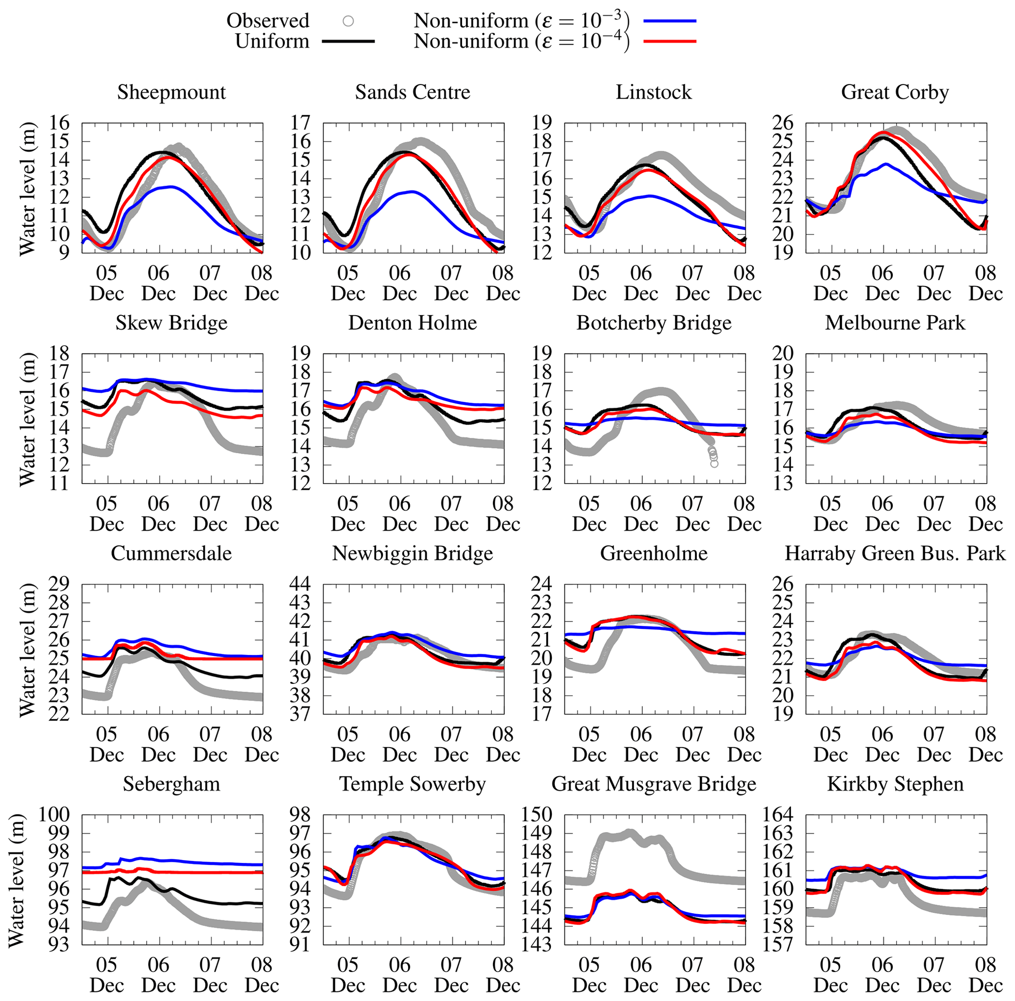
Figure 14Eden catchment. Water level time series predicted by uniform and non-uniform solvers and the in situ measurements at 16 gauge points (marked in Fig. 12).
The impact on accuracy associated with this choice for ε can also be clearly noted in the comparison of the predicted differences in the maximum flood extents with respect to that predicted by the uniform solver (Fig. 15). As can be seen in Fig. 15a, the reference prediction by the uniform grid solver predicts extents that compare reasonably well with the surveyed extent. With , the non-uniform grid solver delivers a competitive prediction to flood extent compared to the uniform grid solver as it achieved very close scores for H, C and F, of 0.95, 0.93 and 0.05, respectively, with minor overpredictions (blue-coloured) towards the easternmost side of the city area and minor underprediction elsewhere (red-coloured). The H, C and F scores became significantly lower with , namely for H and C, of 0.72 and 0.67, indicating further 25 % loss in accuracy of the flood extent prediction, visible by the dominance of underpredictions (red-coloured) in the capture of the main flood extent within the city area (Fig. 15c).
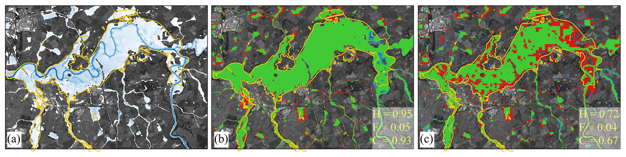
Figure 15Eden catchment. Maximum flood extents predicted by (a) the uniform grid solver and the predicted differences with respect to the non-uniform grid solver using (b) and (c) : green parts flag flooded areas predicted by both the uniform and the non-uniform grid solvers, blue parts flag an overprediction (i.e. flooded areas only predicted by the non-uniform grid solver), and red parts flag an underprediction (i.e. flooded areas only predicted by the uniform grid solver). For reference, the orange line border represents the measured flood extent from the Environment Agency. The hit rate (H), false alarm (F) and critical success index (C) values are computed against the flood extent predicted by the uniform grid solver. © Google Earth 2021.
In terms of speed-up, the uniform grid solver on the GPU architecture is found to be 28 times faster to run than the CPU architecture. This speed-up is somewhat 1 order of magnitude higher than for the previous case study (Sect. 3.2), which is expected as the number of elements on the uniform grid here is more than double (i.e. 6.2 million versus 2.7 million for Upper Lee catchment). With , the non-uniform grid solver adds on a speed-up of around 4 times, associated with a 36 % reduction in the number of elements, whereas, with , the reduction is 85 %, and this further boosts the solver's speed-up to around 12 times. Nonetheless, choosing is necessary with the non-uniform grid solver for such a large-scale simulation at a 20 m DEM resolution to keep acceptable accuracy while benefiting from a considerable speed-up.
Overall, the uniform grid solver on GPU architecture is a promising alternative to boost runtime efficiency for catchment-scale flood simulations that entail large numbers of elements. This efficiency gain can be further enhanced using the non-uniform grid solver, albeit with for the range of DEM resolution used for such simulations to keep the resolution coarsening moderate in favour of accuracy. The amount of enhancement in efficiency depends on the reduction in the number of elements, compared to the uniform grid, becoming worth consideration when this reduction is 30 % or higher.
3.4 Glasgow urban area
This case study mimics an urban flood event in a 400 m × 960 m low-lying area in Glasgow, UK, shown in Fig. 16. It is a hypothetical scenario with a DEM at 0.5 m resolution that excludes the fine-scale urban features. Therefore, a 2 m resolution DEM is often used to benchmark flood modelling software (Néelz and Pender, 2013). The flood is driven by rainfall that overwhelms the drainage system. This causes two sources of flooding, including from spatially uniform rainfall occurring between 1 and 4 min, with an intensity of 400 mm h−1. The other source is at the location denoted by “S” in Fig. 16, where flow surcharges from the drainage system, during 23 and 55 min, reaching a peak of 5 m3 s−1, at t=37 min. The area has two different classes of land use: roads and pavements and other land characteristics, represented by nM=0.02 m and nM=0.05 m, respectively. The 5 h simulation starts over an initially dry area, considering closed boundary conditions. The time series of predicted water levels were recorded at nine gauge points which are shown in Fig. 16. As no observation data are available, the predictions from an alternative uniform grid simulation at the 0.5 m resolution were used as reference.
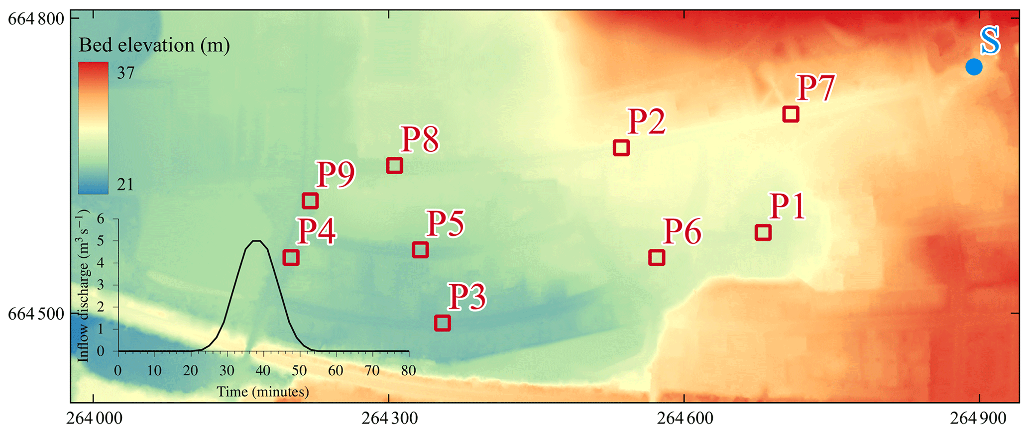
Figure 16Glasgow urban area. Topographic map of the domain, including the positions of the gauge points (P1–P9) and the source inflow (S), with a subfigure showing the inflow hydrograph imposed at point S.
The grids predicted by the non-uniform solver for the two ε values are illustrated in Fig. 17 (upper panels), together with subfigures showing the percentage of coverage for each of the resolutions selected over the area. The finest 2 m resolution is selected in the vicinity of the southern boundary for the two ε values, covering about 20 % and 50 % of the area with and 10−4, respectively. As the DEM lacks fine-scale urban features, the 4 m resolution is selected to cover the majority of the area almost equally with and 10−4, at 60 % and 55 %, respectively. Notably, with , there is more presence of coarser than 4 m resolutions, leading to an overall reduction of 64 % in the number of elements, compared to with that barely uses coarser than 4 m resolution leading to a less reduction of 36 %. This suggests that may be suitable for the non-uniform solver for the 2 m resolution DEM to moderately coarsen its grid while benefiting from a higher reduction for efficiency.
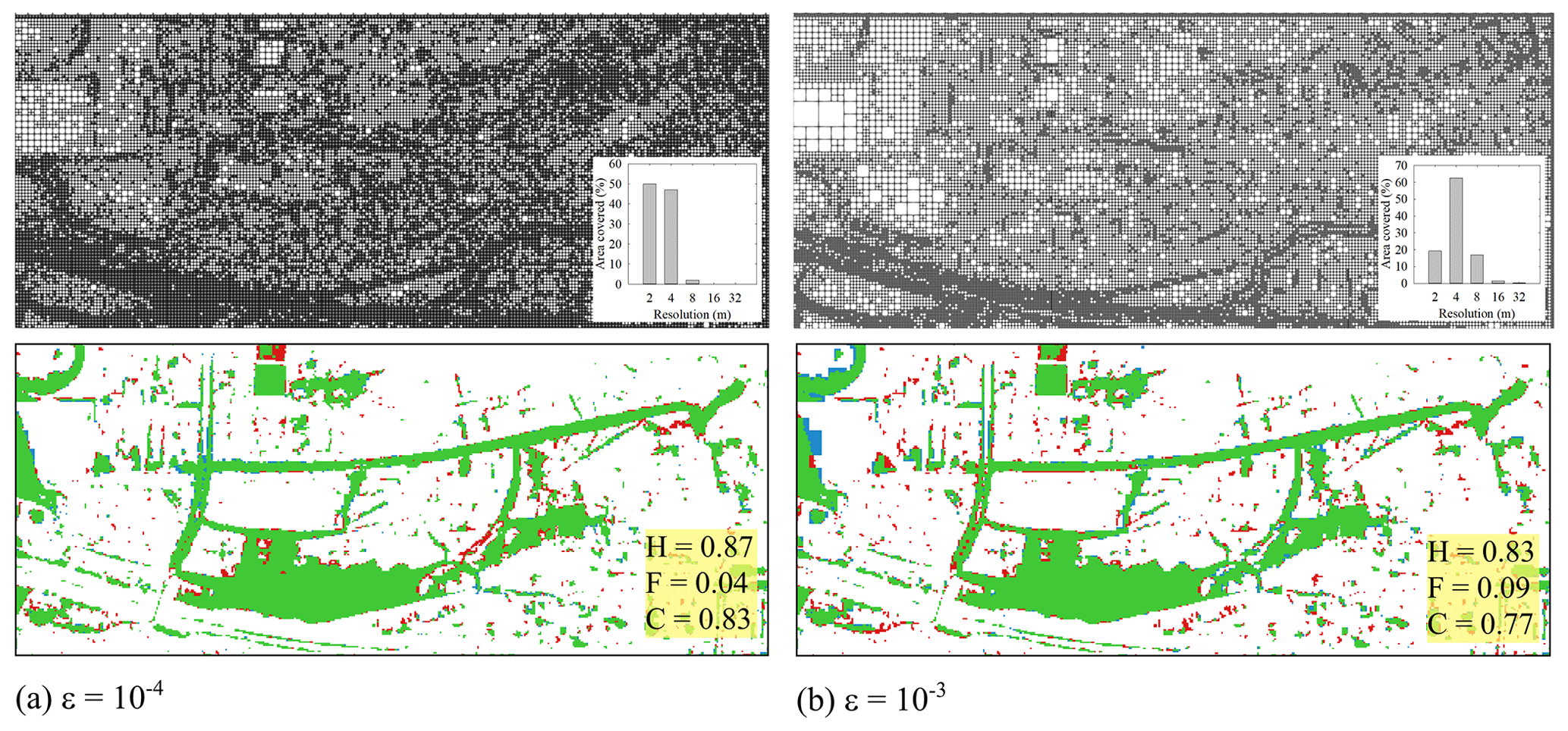
Figure 17Glasgow urban area. Grids generated by the non-uniform solver (upper panels), along with the percentage of the selected resolutions over the urban area, and the differences in the maximum flood extent predicted by the non-uniform grid solver (lower panels), using (a) and (b) . In the lower panels, green parts flag flooded areas predicted by both the uniform and the non-uniform grid solvers, blue parts flag an overprediction (i.e. flooded areas only predicted by the non-uniform grid solver), red parts flag an underprediction (i.e. flooded areas only predicted by the uniform grid solver), and white parts flag dry areas predicted by both the uniform and non-uniform solvers. The hit rate (H), false alarm (F) and critical success index (C) values are computed against the flood extent predicted by the uniform grid solver on 2 m resolution DEM.
Figure 17 (lower panels) also compares the accuracy of the non-uniform grid solver with both ε values for the maximum flood extent predictions. The solver with and 10−4 leads to close predictions with only a noticeable difference in the vicinity of the western boundary, where it overpredicts the flood extent with (i.e. blue-coloured areas, with slightly higher F of 0.09) as compared to with (with F=0.04), which can be expected due to relatively coarser resolution therein. The remaining flooded areas are closely predicted with the two ε values (i.e. large green areas), with rather high and similar H values of 0.87 and 0.83, for and , respectively. This confirms that the additional coarsening achieved by the non-uniform grid solver with only introduces an insignificant loss of accuracy and preserves a C score around 0.8.
This accuracy of the non-uniform solver predictions at can be confirmed by comparing the results in Fig. 18, which shows its predicted time series of the water levels to be comparable with those predicted the uniform solver, all agreeing with the reference predictions. At all the gauge points, the non-uniform solver, with both and 10−4, leads to almost similar accuracy compared to uniform solver predictions, successfully reproducing the double peak observed within the reference predictions and other predictions reported in the literature (Néelz and Pender, 2013). Hence, the non-uniform solver, with both and 10−4, is a valid alternative to the uniform solver for such a case study featured by flooded zones within a small domain area with smooth terrain that is, moreover, represented at a fine DEM resolution of 2 m.

Figure 18Glasgow urban area. Water level time series predicted by uniform and non-uniform solvers and reference water levels predicted by the uniform solver on a 0.5 m × 0.5 m grid, at gauge points 1 to 9 (marked in Fig. 16).
In terms of speed-up, the uniform grid solver on the GPU architecture is only 1.4 times faster than the CPU version, which is expected for a number of elements as low as 95 000 as discussed previously (Sect. 3.1). With , the non-uniform grid solver boosts the speed-up to 3.8 times, which in turn increases to 5.3 times with , which entails a higher reduction in the number of elements. All considered, is found to be a valid choice with the non-uniform grid solver for urban resolution flood simulations to both preserve acceptable accuracy and boost efficiency. The relevance of this choice is further investigated next for a realistic case study with an urban resolution DEM that includes small fine-scale topographic features.
3.5 Cockermouth urban area
The case study involves a 144 h fluvial flooding scenario over a 1.42 km2 urban area in the town of Cockermouth, Cumbria, UK. The town is located at the confluence of river Derwent and its tributary, river Cocker (Fig. 19). Like the Eden catchment (Sect. 3.3), this area was affected by the record-breaking rainfall from Storm Desmond in 2015 that manifested in a water level increase of the river Derwent that caused river waters to inundate the town (Met Office, 2018). Measured time series of the volumetric flow at 15 min intervals (from 3 December 2015 to 9 December 2015) were available at Southwaite Bridge and Ouse Bridge for the river Cocker and river Derwent, respectively (Environment Agency, 2018). As these two locations are considerably farther from the boundaries, the inflow hydrographs at rivers Cocker and Derwent were calibrated (Muthusamy et al., 2021) and imposed (at the two associated points shown in Fig. 19). Here, the 1 m resolution DEM is inclusive of the fine-scale urban features. Two different values were used for the friction parameter, nM=0.035 and 0.05 m for river channels and floodplains, respectively. The northern, southern and eastern boundaries are set as closed, while a free outflow boundary condition is allowed at the downstream of river Derwent. There are two gauge points on the rivers, located at P1 (river Cocker) and P2 (river Derwent), marked in Fig. 19, where water depths predicted by the solvers were recorded to compare with existing in situ measurements.
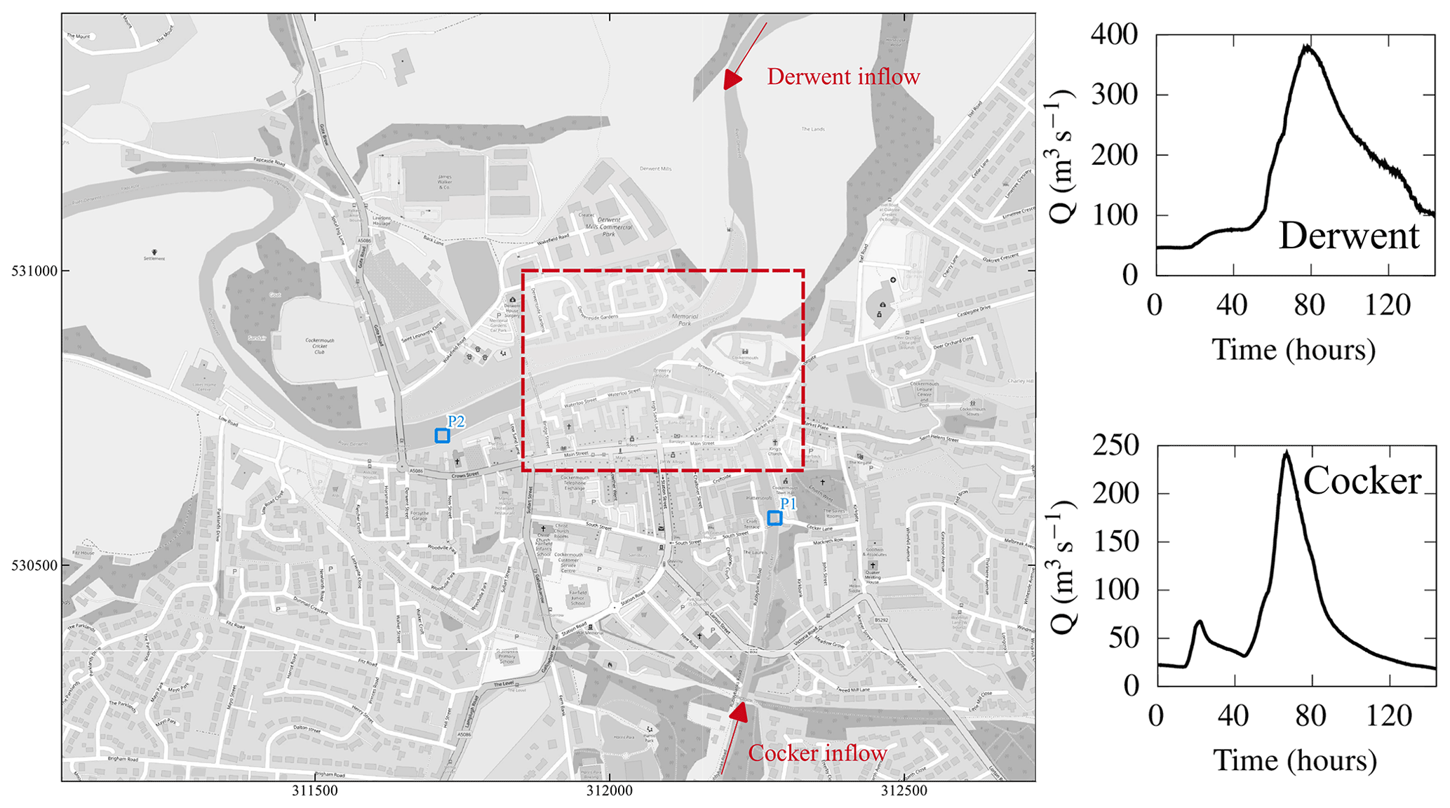
Figure 19Cockermouth urban area. The study area and the positions of the gauge points P1 and P2. The arrows show the positions where the inflow hydrographs are imposed upstream of the rivers Derwent and Cocker. The dashed line frames a smaller portion of the domain where the generated grids are compared. © OpenStreetMap contributors 2021. Distributed under the Open Data Commons Open Database License (ODbL) v1.0.
Figure 20 compares the generated non-uniform grids using two ε values over the smaller portion of the domain framed in Fig. 19, along with subfigures showing the percentage of the resolutions covering the whole study area. As shown in Fig. 20a, the choice of leads to an overly refined grid, where over 50 % of the area is covered with the finest 1 m resolution, entailing a 37 % reduction in the number of elements. Comparatively, as shown in Fig. 20b, leads to a more sensible resolution selection as the finest 1 m resolution is only present around the urban features (e.g. the buildings), while resolutions up to three levels coarser, i.e. 8 m, are selected over the pathways, and even coarser resolutions, between 16 and 32 m, are selected over the river channels. This leads to a reduction of 60 % associated with a wider range and more evenly distributed resolution selection compared to the smaller choice of (see the subfigures in Fig. 20).
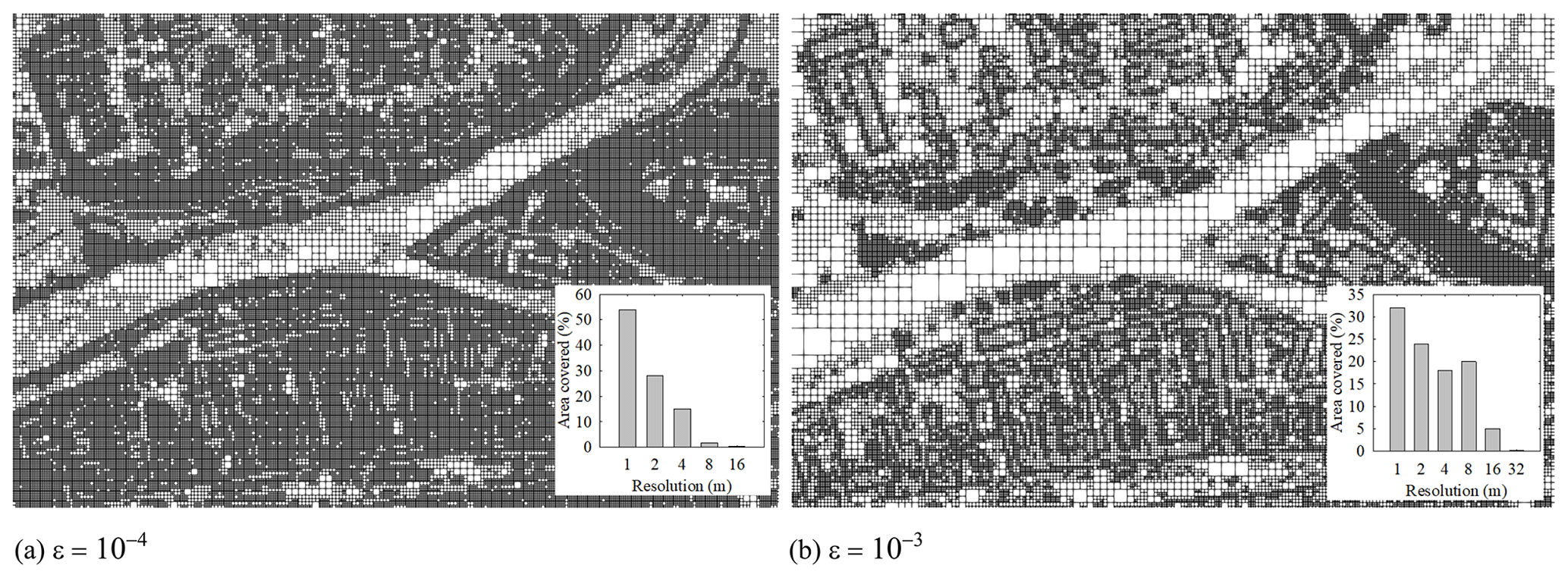
Figure 20Cockermouth urban area. Grids generated by the non-uniform solver using (a) and (b) , over the smaller portion of the domain framed in Fig. 19, along with the percentage of the selected resolutions over the whole urban area.
Figure 21 assesses the accuracy of the non-uniform grid solver with both ε values in terms of water depth hydrograph predictions at gauge points P1 and P2 (Fig. 21a–b) and maximum flood extent (Fig. 21c–e) predictions, with reference to the predictions made by the uniform grid solver, while comparting with measured hydrographs and a surveyed flood extent, respectively. As can be seen in Fig. 21a and b, the hydrograph predictions by the uniform grid solver follow the rising limb of the measured hydrograph up to the peak of the hydrograph at 70 h, where it only shows a 20 cm underprediction. Also, the uniform grid solver could correctly capture the falling limb, with a slightly more gradual decrease from the measured hydrographs. The hydrographs predicted by the non-uniform grid solver with the two ε values are very close to those predicted by the uniform solver with a negligible difference that likely occurs from the accumulation of numerical diffusion due to the coarser resolutions on the non-uniform grids (Kesserwani and Sharifian, 2023). This suggests that the predictability of the present non-uniform solver to short-timescale events improves with increased refinement of the DEM resolution (namely as small as 1 m for this case study).
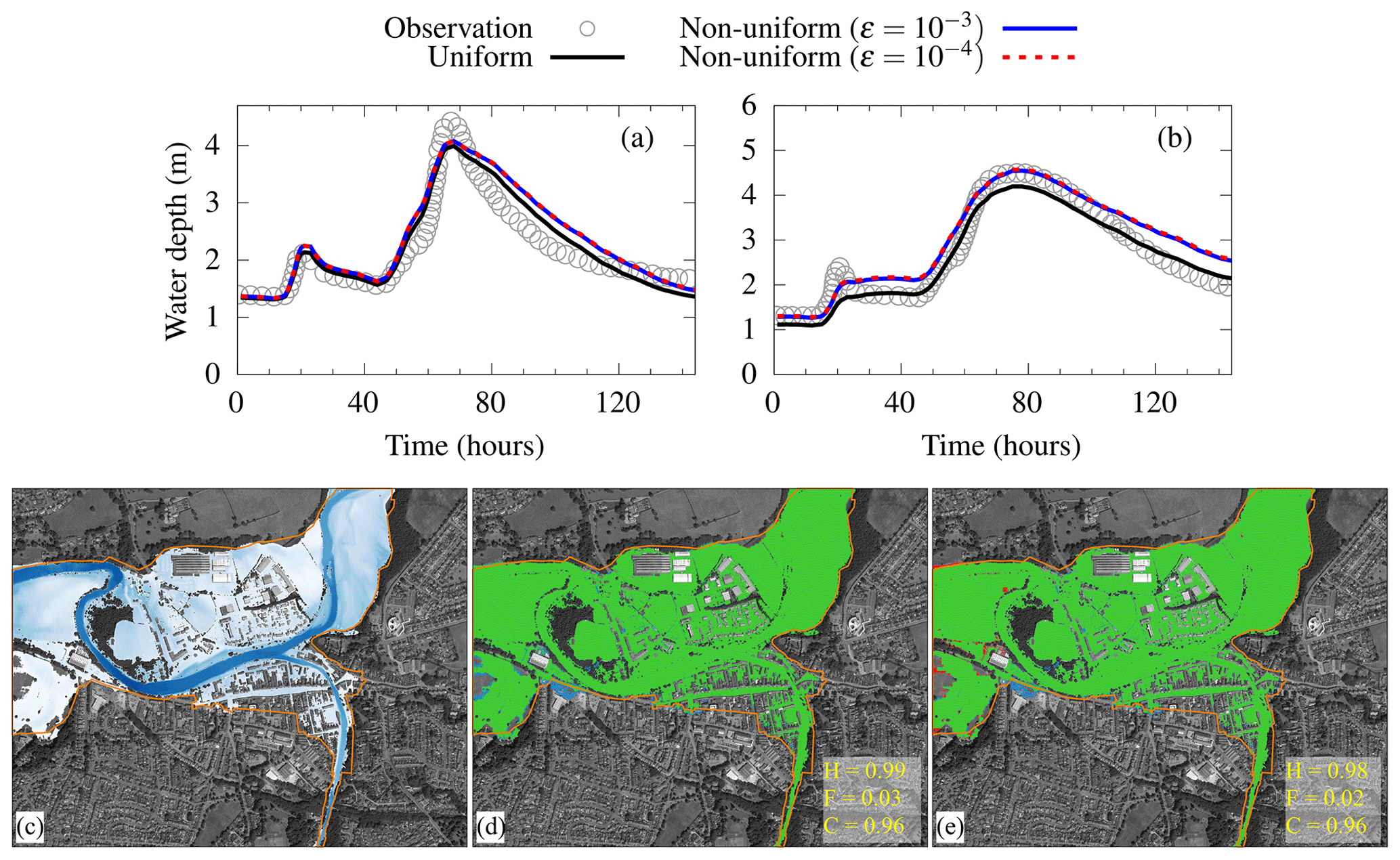
Figure 21Cockermouth urban area. Water level time series predicted by uniform and non-uniform solvers compared to the in situ-measured water levels at locations (a) P1 (river Cocker) and (b) P2 (river Derwent). Maximum flood extents predicted by (c) the uniform grid solver and the predicted differences with respect to the non-uniform grid solver using (d) and (e) : green parts flag flooded areas predicted by both the uniform and the non-uniform grid solvers, blue parts flag an overprediction (i.e. flooded areas only predicted by the non-uniform grid solver), and red parts flag an underprediction (i.e. flooded areas only predicted by the uniform grid solver). For reference, the orange line border represents the measured flood extent from the Environment Agency. The hit rate (H), false alarm (F) and critical success index (C) values are computed against the flood extent predicted by the uniform grid solver. © Google Earth 2021.
The equally good accuracy for the non-uniform solver predictions with the two ε values can also be confirmed by the fact that their predicted maximum flood extents (Fig. 21d and e) are visually comparable (green-coloured areas) to the one predicted by the uniform grid solver (Fig. 21c) that in turn agrees well with the surveyed extent (Environment Agency, 2018). The accuracy of the non-uniform solver prediction can be quantitatively confirmed by computing the H, F and C metrics with reference to the predicted maximum flood extent by the uniform solver. The scores for H, F and C achieved by the non-uniform grid solver with and are very similar, with a C value exceeding 0.9, suggesting very close accuracy in the flood extent predicted by the uniform grid solver. As opposed to the case study of the Glasgow urban area (Sect. 3.4), the C score, of 0.96, is preserved despite increasing ε from 10−4 to 10−3, but this is more related to the fact that there is one consolidated flooded zone occurring in a small-perimeter area represented at a 1 m DEM resolution.
In terms of speed-up, the uniform grid solver on GPU architecture ran 8.9 times faster than the CPU architecture. This is in line with the previous findings (Sect. 3.1 to 3.3), as more than 1 million elements were involved in the grid for this case study, confirming the utility of the GPU architecture to run faster simulations with a large number of elements. However, this gain in speed-up can get compromised when using the non-uniform grid solver. With , the non-uniform grid solver is in fact a bit slower (1.1 times) than the uniform grid solver, which may be expected as the grid is dominated by the finest resolution (Fig. 20a) with 37 % reduction. Remarkably, with , which led to a much coarser grid with a 60 % reduction, the speed-up is insignificant, only 1.2 times faster than the uniform grid solver. This little gain in speed-up could be explained by contrasting the depth, variability and distribution of the resolutions selected on the non-uniform grids to those in the other case studies (Sect. 3.1 to 3.4). It can be noted that the non-uniform grids in the other case studies are featured by the dominance of one or at most two resolutions, depending on the choice of ε. This means that the non-uniform grid solver has more access to regularly sized neighbours, which helps maximise its efficiency. In contrast, the grids here are featured by more depth and variability in resolution, selected with quite an even distribution, in particular with (Fig. 20b). This culminates in a high number of differently sized elements, causing an overhead in the solver calculation at those elements surrounded by too many neighbouring elements with different sizes. Such a knock-on effect on the efficiency of the non-uniform solver would be expected to increasingly reduce as the modelled area of interest is larger and more inclusive of rural surroundings at coarser resolutions. Still, the speed-up analysis confirms that the non-uniform solver with is a good choice for urban-scale simulations, to keep close accuracy to the uniform solver on GPU architecture and remain more efficient. As the modelled area of interest becomes smaller, and the terrain features are well resolved in the DEM, the efficiency gain over the uniform solver may not be substantial, and this makes it a competitive first choice for such a type of urban-scale simulations.
The two-dimensional ACCeleration (ACC) uniform grid solver has been widely used to run efficient simulations for a wide range of flood modelling applications. The efficiency of the ACC solver is owed to a reduced form of the shallow water equations solved by a simple numerical scheme and optimisation measures for the central processing unit (CPU) architecture with effective handling of wet–dry zones. This paper presented two potentially faster versions that run on the graphical processing unit (GPU): a uniform grid version built on the existing codebase (Shaw et al., 2021) and a non-uniform grid version within an ad hoc codebase, with guidance on how to set up and run these new versions, at https://www.seamlesswave.com/LISFLOOD8.0 (last access: 28 April 2023).
Table 4Summary of best-practice recommendations for using uniform and non-uniform solvers on GPUs.
The non-uniform solver has a grid generator that uses the multiresolution analysis (MRA) of the multiwavelets to a planar Galerkin projection of the digital elevation model (DEM), while only requiring one user-specified parameter of an error threshold, ε, in the vicinity of 10−3 (Kesserwani and Sharifian, 2020). This threshold enables us to sensibly coarsen the resolutions on the grid and to properly distribute different classes of Manning's parameters at the coarsened elements. The ACC solver's scheme is adapted to aggregate the discharges across non-uniformly sized grid elements. Both the grid generator and the adapted scheme are implemented in a new codebase to efficiently run on the GPU architecture.
The performance of the GPU versions of the uniform and non-uniform grid solvers was assessed for five pluvial/fluvial flooding case studies at the catchment and urban scale. The non-uniform solver simulations were run for two ε values, 10−3 and 10−4, according to which accuracy was measured in terms of prediction closeness to the simulations by the uniform solver run at DEM resolution. The speed-up gained by using the GPU version of the uniform solver, over the CPU version, was quantified using the ratio of runtimes with reference to the number of elements on the grid. Similarly, the enhancement in speed-up from using the non-uniform solver over the uniform solver on the GPU was quantified with reference to the relative reduction in the number of elements on the non-uniform grid.
For the catchment-scale simulations at DEM resolution as coarse as 10 m or higher, the non-uniform solver with generated grids without excessive resolution coarsening leading to acceptable accuracy. For such simulations, led to deterioration in accuracy due to excessively coarsened elements on the non-uniform grid, yielding resolutions that were too much coarser than the resolution of the DEM, and is therefore not recommended. For the urban-scale simulations at DEM resolutions as fine as 2 m or lower, both ε values were found valid for use with the non-uniform solver to preserve accuracy, but was found to lead to a more sensible coarsening in the resolution on the non-uniform grid. One important factor to note for the ACC solver's simplified formulation, when applied for catchment-scale simulations, is the potential instabilities that could result from modelling thin, fast-flowing water depths. Such instabilities can particularly happen when modelling pluvial floods over steeply varying, fine-resolution topographies, requiring extra measures to suppress them such as introducing artificial numerical diffusion in an adaptive manner (e.g. as in Sridharan et al., 2021).
In terms of speed-ups, the GPU version of the uniform grid solver was increasingly faster to run than the CPU version as the number of elements on the grid became increasingly larger, reaching up to 28 times on a grid with 6 million elements. On the GPU, the non-uniform solver could offer further enhancements in speed-up, depending on the DEM resolution and the properties of the case study. For coarse DEM resolutions featuring the catchment-scale simulations at the recommended , the speed-up enhancement increased with more reduction in the number of elements, reaching up to 4 times for a reduction of 36 %. A similar enhancement was identified at finer DEM resolution featuring the urban-scale simulations at the recommended , albeit at a higher reduction, exceeding 65 %, when the grid was dominated by at most two resolutions. The enhancement became moderate to insignificant when there was more depth and breadth in resolutions with even distributions, which is likely the case where the GPU version of the uniform solver should be preferred. Table 4 summarises the best-practice recommendations drawn from this study to choose the most suitable ACC solver for modelling fluvial/pluvial flooding scenarios, considering the number of elements required for the uniform grid to achieve considerable GPU speed-up, alongside the ε value for the non-uniform solver.
LISFLOOD-FP8.1 source code (LISFLOOD-FP developers, 2022; https://doi.org/10.5281/zenodo.6912932) and simulation results (Sharifian et al., 2022; https://doi.org/10.5281/zenodo.6907286) are available from Zenodo. Due to access restrictions, readers are invited to contact the Environment Agency for access to the data used in Sect. 3.4 and to refer to the cited references for the data used in Sect. 3.1, 3.2, 3.3 and 3.5.
Step-by-step instructions on how to download and install LISFLOOD-FP8.1 and reproduce the simulations for representative case studies (Sect. 3.2 and 3.4) are available from Zenodo at https://doi.org/10.5281/zenodo.6685125 (Sharifian and Kesserwani, 2022).
MKS coded the numerical solvers in collaboration with AAC and JN. MKS and GK were responsible for the conceptualisation, methodology, formal analysis, investigation, visualisation and writing the initial draft. All authors contributed to paper review and editing.
At least one of the (co-)authors is a member of the editorial board of Geoscientific Model Development. The peer-review process was guided by an independent editor, and the authors also have no other competing interests to declare.
Publisher’s note: Copernicus Publications remains neutral with regard to jurisdictional claims in published maps and institutional affiliations.
We wish to thank Ilhan Özgen-Xian (Technische Universität Braunschweig) for sharing the data for the Lower Triangle catchment case study and for the constructive review of the manuscript and Xilin Xia (Loughborough University) for sharing the data for Upper Lee and Eden catchment case studies. This work is part of the SEAMLESS-WAVE project (SoftwarE infrAstructure for Multi-purpose fLood modElling at various scaleS based on WAVElets; https://www.seamlesswave.com, last access: 28 April 2023).
Mohammad Kazem Sharifian, Georges Kesserwani and Alovya Ahmed Chowdhury were supported by the UK Engineering and Physical Sciences Research Council (EPSRC) grant EP/R007349/1. Jeff Neal was funded by the Natural Environment Research Council (NERC) grant NE/S006079/1. Paul Bates was supported by a Royal Society Wolfson Research Merit award.
This paper was edited by Lutz Gross and reviewed by Ilhan Özgen-Xian and one anonymous referee.
Amarnath, G., Umer, Y. M., Alahacoon, N., and Inada, Y.: Modelling the flood-risk extent using LISFLOOD-FP in a complex watershed: case study of Mundeni Aru River Basin, Sri Lanka, Proc. Intl. Assoc. Hydrol. Sci., 370, 131–138, 2015.
Asinya, E. A. and Alam, M. J. B.: Flood risk in rivers: climate driven or morphological adjustment, Earth Syst. Env., 5, 861–871, 2021.
Bates, P. D. and De Roo, A. P. J.: A simple raster-based model for flood inundation simulation, J. Hydrol., 236, 54–77, 2000.
Bates, P. D., Horritt, M. S., and Fewtrell, T. J.: A simple inertial formulation of the shallow water equations for efficient two-dimensional flood inundation modelling, J. Hydrol., 387, 33–45, 2010.
Beevers, L., Collet, L., Aitken, G., Maravat, C., and Visser, A.: The influence of climate model uncertainty on fluvial flood hazard estimation, Nat. Hazards, 104, 2489–2510, 2020.
Bessar, M. A., Choné, G., Lavoie, A., Buffin-Bélanger, T., Biron, P. M., Matte, P., and Anctil, F.: Comparative analysis of local and large-scale approaches to floodplain mapping: a case study of the Chaudière River, Canadian Wat. Resour., 46, 194–206, 2021.
Chaabani, C., Chini, M., Abdelfattah, R., Hostache, R., and Chokmani, K.: Flood mapping in a complex environment using bistatic TanDEM-X/TerraSAR-X InSAR coherence, Remote Sens., 10, 1873, https://doi.org/10.3390/rs10121873, 2018.
Choné, G., Biron, P. M., Buffin‐Bélanger, T., Mazgareanu, I., Neal, J. C., and Sampson, C. C.: An assessment of large‐scale flood modelling based on LiDAR data, Hydrol. Process., 35, e14333, https://doi.org/10.1002/hyp.14333, 2021.
Chow, V. T.: Open Channel Hydraulics, McGraw-Hill, New York, ISBN 007085906X, 9780070859067, 1959.
Costabile, P., Costanzo, C., Ferraro, D., and Barca, P.: Is HEC-RAS 2D accurate enough for storm-event hazard assessment? Lessons learnt from a benchmarking study based on rain-on-grid modelling, J. Hydrol., 603, 126962, https://doi.org/10.1016/j.jhydrol.2021.126962, 2021.
Coulthard, T. J., Neal, J. C., Bates, P. D., Ramirez, J., de Almeida, G. A., and Hancock, G. R.: Integrating the LISFLOOD-FP 2D hydrodynamic model with the CAESAR model: implications for modelling landscape evolution, Earth Surf. Process. Landform., 38, 1897–1906, 2013.
De Almeida, G. A. and Bates, P.: Applicability of the local inertial approximation of the shallow water equations to flood modelling, Water Resour. Res., 49, 4833–4844, 2013.
De Almeida, G. A. M., Bates, P., Freer, J. E., and Souvignet, M.: Improving the stability of a simple formulation of the shallow water equations for 2-D flood modeling, Water Resour. Res., 48, W05528, https://doi.org/10.1029/2011WR011570, 2012.
Environment Agency: Real-time and Near-real-time river level data, Environment Agency [data set], https://data.gov.uk/dataset/0cbf2251-6eb2-4c4e-af7c-d318da9a58be/real-time-and-near-real-time-river-level-data (last access: 28 April 2023), 2020.
Ferraro, D., Costabile, P., Costanzo, C., Petaccia, G., and Macchione, F.: A spectral analysis approach for the a priori generation of computational grids in the 2-D hydrodynamic-based runoff simulations at a basin scale, J. Hydrol., 582, 124508, https://doi.org/10.1016/j.jhydrol.2019.124508, 2020.
Guo, K., Guan, M., and Yu, D.: Urban surface water flood modelling – a comprehensive review of current models and future challenges, Hydrol. Earth Syst. Sci., 25, 2843–2860, https://doi.org/10.5194/hess-25-2843-2021, 2021.
Hirai, S. and Yasuda, T.: Risk assessment of aggregate loss by storm surge inundation in ise and mikawa bay, in: Coastal Engineering Proceedings: No. 36 (2018): Proceedings of 36th Conference on Coastal Engineering, Baltimore, Maryland, 30 July–3 August 2018, https://doi.org/10.9753/icce.v36.risk.35, 2018.
Hoch, J. M. and Trigg, M. A.: Advancing global flood hazard simulations by improving comparability, benchmarking, and integration of global flood models, Environ. Res. Lett., 14, 034001, https://doi.org/10.1088/1748-9326/aaf3d3, 2019.
Hoch, J. M., Eilander, D., Ikeuchi, H., Baart, F., and Winsemius, H. C.: Evaluating the impact of model complexity on flood wave propagation and inundation extent with a hydrologic–hydrodynamic model coupling framework, Nat. Hazards Earth Syst. Sci., 19, 1723–1735, https://doi.org/10.5194/nhess-19-1723-2019, 2019.
Hunter, N. M., Horritt, M. S., Bates, P. D., Wilson, M. D., and Werner, M. G.: An adaptive time step solution for raster-based storage cell modelling of floodplain inundation, Adv. Water Resour., 28, 975–991, 2005.
Hunter, N. M., Bates, P. D., Horritt, M. S., and Wilson, M. D.: Improved simulation of flood flows using storage cell models, in: Proceeds. Instit. Civil Engs. Water Manag., Vol. 159, No. 1, 9–18, Thomas Telford Ltd, https://doi.org/10.1680/wama.2006.159.1.9, 2006.
Hunter, N. M., Bates, P. D., Neelz, S., Pender, G., Villanueva, I., Wright, N. G., Liang, D., Falconer, R. A., Lin, B., Waller, S., Crossley, A. J., and Mason, D. C.: Benchmarking 2D hydraulic models for urban flooding, in: Proceeds. Inst. Civil Engs. Water Manag., Vol. 161, No. 1, 13–30, Thomas Telford Ltd, https://doi.org/10.1680/wama.2008.161.1.13, 2008.
Jafarzadegan, K., Abbaszadeh, P., and Moradkhani, H.: Sequential data assimilation for real-time probabilistic flood inundation mapping, Hydrol. Earth Syst. Sci., 25, 4995–5011, https://doi.org/10.5194/hess-25-4995-2021, 2021.
Karamouz, M. and Mahani, F. F.: DEM uncertainty based coastal flood inundation modeling considering water quality impacts, Water Resour. Manag., 35, 3083–3103, 2021.
Kesserwani, G. and Sharifian, M. K.: (Multi)wavelets increase both accuracy and efficiency of standard Godunov-type hydrodynamic models: Robust 2D approaches, Adv. Water Resour., 144, 103693, https://doi.org/10.1016/j.advwatres.2020.103693, 2020.
Kesserwani, G. and Sharifian, M. K.: (Multi) wavelet-based Godunov-type simulators of flood inundation: Static versus dynamic adaptivity, Adv. Water Resour., 171, 104357, https://doi.org/10.1016/j.advwatres.2022.104357, 2023.
Kesserwani, G., Shaw, J., Sharifian, M. K., Bau, D., Keylock, C. J., Bates, P. D., and Ryan, J. K.: (Multi)wavelets increase both accuracy and efficiency of standard Godunov-type hydrodynamic models, Adv. Water Resour., 129, 31–55, https://doi.org/10.1016/j.advwatres.2019.04.019, 2019.
LISFLOOD-FP developers: LISFLOOD-FP 8.1 hydrodynamic model (8.1), Zenodo [code], https://doi.org/10.5281/zenodo.6912932, 2022.
Liu, Z. and Merwade, V.: Accounting for model structure, parameter and input forcing uncertainty in flood inundation modeling using Bayesian model averaging, J. Hydrol., 565, 138–149, 2018.
Makungu, E. and Hughes, D. A.: Understanding and modelling the effects of wetland on the hydrology and water resources of large African river basins, J. Hydrol., 603, 127039, https://doi.org/10.1016/j.jhydrol.2021.127039, 2021.
McCall, I.: Carlisle Flood Investigation Report, Flood Event 5–6th December 2015, Tech. Rep., Environment Agency, https://www.cumbria.gov.uk/eLibrary/Content/Internet/536/6181/42494151257.pdf (last access: 28 April 2023), 2016.
Met Office: Met Office Rain Radar Data from the NIMROD System, Met Office [data set], https://catalogue.ceda.ac.uk/uuid/82adec1f896af6169112d09cc1174499 (last access: 28 April 2023), 2013.
Ming, X., Liang, Q., Xia, X., Li, D., and Fowler, H. J.: Real‐time flood forecasting based on a high‐performance 2‐D hydrodynamic model and numerical weather predictions, Water Resour. Res., 56, e2019WR025583, https://doi.org/10.1029/2019WR025583, 2020.
Muthusamy, M., Casado, M. R., Butler, D., and Leinster, P.: Understanding the effects of Digital Elevation Model resolution in urban fluvial flood modelling, J. Hydrol., 596, 126088, https://doi.org/10.1016/j.jhydrol.2021.126088, 2021.
Nandi, S. and Reddy, M. J.: An integrated approach to streamflow estimation and flood inundation mapping using VIC, RAPID and LISFLOOD-FP, J. Hydrol., 610, 127842, https://doi.org/10.1016/j.jhydrol.2022.127842, 2022.
Neal, J., Schumann, G., and Bates, P.: A subgrid channel model for simulating river hydraulics and floodplain inundation over large and data sparse areas, Water Resour. Res., 48, W11506, https://doi.org/10.1029/2012WR012514, 2012a.
Neal, J., Villanueva, I., Wright, N., Willis, T., Fewtrell, T., and Bates, P.: How much physical complexity is needed to model flood inundation?, Hydrol. Process., 26, 2264–2282, 2012b.
Neal, J., Dunne, T., Sampson, C., Smith, A., and Bates, P.: Optimisation of the two-dimensional hydraulic model LISFOOD-FP for CPU architecture, Environ. Modell. Softw., 107, 148–157, 2018.
Néelz, S. and Pender, G.: Benchmarking the latest generation of 2D hydraulic modelling packages, Tech. Rep. SC120002, Environment Agency, Horizon House, Deanery Road, Bristol, BS1 9AH, https://www.gov.uk/government/publications/benchmarking-the-latest-generation-of-2d-hydraulic-flood-modelling-packages (last access: 28 April 2023), 2013.
O'Loughlin, F. E., Neal, J., Schumann, G. J. P., Beighley, E., and Bates, P. D.: A LISFLOOD-FP hydraulic model of the middle reach of the Congo, J. Hydrol., 580, 124203, https://doi.org/10.1016/j.jhydrol.2019.124203, 2020.
Özgen-Xian, I., Kesserwani, G., Caviedes-Voullième, D., Molins, S., Xu, Z., Dwivedi, D., David Moulton, J., and Steefel, C. I.: Wavelet-based local mesh refinement for rainfall-runoff simulations, J. Hydroin., 22, 1059–1077, 2020.
Rajib, A., Liu, Z., Merwade, V., Tavakoly, A. A., and Follum, M. L.: Towards a large-scale locally relevant flood inundation modeling framework using SWAT and LISFLOOD-FP, J. Hydrol., 581, 124406, https://doi.org/10.1016/j.jhydrol.2019.124406, 2020.
Seenath, A.: Effects of DEM resolution on modeling coastal flood vulnerability, Mar. Geod., 41, 581–604, https://doi.org/10.1080/01490419.2018.1504838, 2018.
Sharifian, M. K. and Kesserwani, G.: LISFLOOD-FP 8.1: New GPU accelerated solvers for faster fluvial/pluvial flood simulations – video supplement, Zenodo [video], https://doi.org/10.5281/zenodo.6685125, 2022.
Sharifian, M. K., Kesserwani, G., Chowdhury, A. A., Neal, J., and Bates, P.: LISFLOOD-FP 8.1: New GPU accelerated solvers for faster fluvial/pluvial flood simulations – simulation results, Zenodo [data set], https://doi.org/10.5281/zenodo.6907286, 2022.
Shaw, J., Kesserwani, G., Neal, J., Bates, P., and Sharifian, M. K.: LISFLOOD-FP 8.0: the new discontinuous Galerkin shallow-water solver for multi-core CPUs and GPUs, Geosci. Model Dev., 14, 3577–3602, https://doi.org/10.5194/gmd-14-3577-2021, 2021.
Shustikova, I., Neal, J. C., Domeneghetti, A., Bates, P. D., Vorogushyn, S., and Castellarin, A.: Levee breaching: a new extension to the LISFLOOD-FP model, Water, 12, 942, https://doi.org/10.3390/w12040942, 2020.
Siqueira, V. A., Paiva, R. C. D., Fleischmann, A. S., Fan, F. M., Ruhoff, A. L., Pontes, P. R. M., Paris, A., Calmant, S., and Collischonn, W.: Toward continental hydrologic–hydrodynamic modeling in South America, Hydrol. Earth Syst. Sci., 22, 4815–4842, https://doi.org/10.5194/hess-22-4815-2018, 2018.
Sosa, J., Sampson, C., Smith, A., Neal, J., and Bates, P.: A toolbox to quickly prepare flood inundation models for LISFLOOD-FP simulations, Env. Modell. Soft., 123, 104561, https://doi.org/10.1016/j.envsoft.2019.104561, 2020.
Sridharan, B., Bates, P. D., Sen, D., and Kuiry, S. N.: Local-inertial shallow water model on unstructured triangular grids, Adv. Water Resour., 152, 103930, https://doi.org/10.1016/j.advwatres.2021.103930, 2021.
Taccone, F., Antoine, G., Delestre, O., and Goutal, N.: A new criterion for the evaluation of the velocity field for rainfall-runoff modelling using a shallow-water model, Adv. Water Resour., 140, 103581, https://doi.org/10.1016/j.advwatres.2020.103581, 2020.
Towner, J., Cloke, H. L., Zsoter, E., Flamig, Z., Hoch, J. M., Bazo, J., Coughlan de Perez, E., and Stephens, E. M.: Assessing the performance of global hydrological models for capturing peak river flows in the Amazon basin, Hydrol. Earth Syst. Sci., 23, 3057–3080, https://doi.org/10.5194/hess-23-3057-2019, 2019.
Wainwright, H. and Williams, K.: LiDAR collection in August 2015 over the East River Watershed, Colorado, USA, Watershed Function SFA, ESS-DIVE repository [data set], https://doi.org/10.21952/WTR/1412542 (last access: 19 February 2023), 2017.
Wang, Y., Liang, Q., Kesserwani, G., and Hall, J. W.: A positivity-preserving zero-inertia model for flood simulation, Comp. Fluids, 46, 505–511, 2011.
Wing, O. E. J., Bates, P. D., Sampson, C. C., Smith, A. M., Johnson, K. A., and Erickson, T. A.: Validation of a 30 m resolution flood hazard model of the conterminous United States, Water Resour. Res., 53, 7968–7986, 2017.
Wu, X., Wang, Z., Guo, S., Lai, C., and Chen, X.: A simplified approach for flood modeling in urban environments, Hydrol. Res., 49, 1804–1816, 2018.
Xia, X. and Liang, Q.: A new efficient implicit scheme for discretising the stiff friction terms in the shallow water equations, Adv. Water Resour., 117, 87–97, 2018.
Xia, X., Liang, Q., and Ming, X.: A full-scale fluvial flood modelling framework based on a high-performance integrated hydrodynamic modelling system (HiPIMS), Adv. Water Resour., 132, 103392, https://doi.org/10.1016/j.advwatres.2019.103392, 2019.
Yang, Q., Ma, Z., and Zhang, S.: Urban Pluvial Flood Modeling by Coupling Raster-Based Two-Dimensional Hydrodynamic Model and SWMM, Water, 14, 1760, https://doi.org/10.3390/w14111760, 2022.
Yin, Y., Val, D. V., Zou, Q., and Yurchenko, D.: Resilience of Critical Infrastructure Systems to Floods: A Coupled Probabilistic Network Flow and LISFLOOD-FP Model, Water, 14, 683, https://doi.org/10.3390/w14050683, 2022.
Zare, M., Schumann, G. J. P., Teferle, F. N., and Mansorian, R.: Generating Flood Hazard Maps Based on an Innovative Spatial Interpolation Methodology for Precipitation, Atmosphere, 12, 1336, https://doi.org/10.3390/atmos12101336, 2021.
Zeng, Z., Wang, Z., and Lai, C.: Simulation Performance Evaluation and Uncertainty Analysis on a Coupled Inundation Model Combining SWMM and WCA2D, Int. J. Dis. Risk Sci., 13, 448–464, https://doi.org/10.1007/s13753-022-00416-3, 2022.
Zhao, G., Bates, P., and Neal, J.: The impact of dams on design floods in the conterminous US, Water Resour. Res., 56, e2019WR025380, https://doi.org/10.1029/2019WR025380, 2020.
Zhao, J., Pelich, R., Hostache, R., Matgen, P., Wagner, W., and Chini, M.: A large-scale 2005–2012 flood map record derived from ENVISAT-ASAR data: United Kingdom as a test case, Remote Sens. Env., 256, 112338, https://doi.org/10.1016/j.rse.2021.112338, 2021.
Zhu, S., Dai, Q., Zhao, B., and Shao, J.: Assessment of population exposure to urban flood at the building scale, Water, 12, 3253, https://doi.org/10.3390/w12113253, 2020.
Zhu, X., Dai, Q., Han, D., Zhuo, L., Zhu, S., and Zhang, S.: Modeling the high-resolution dynamic exposure to flooding in a city region, Hydrol. Earth Syst. Sci., 23, 3353–3372, https://doi.org/10.5194/hess-23-3353-2019, 2019.
Ziliani, L., Surian, N., Botter, G., and Mao, L.: Assessment of the geomorphic effectiveness of controlled floods in a braided river using a reduced-complexity numerical model, Hydrol. Earth Syst. Sci., 24, 3229–3250, https://doi.org/10.5194/hess-24-3229-2020, 2020.