the Creative Commons Attribution 4.0 License.
the Creative Commons Attribution 4.0 License.
 | 05 May 2023
Emulating aerosol optics with randomly generated neural networks
Po-Lun Ma
Balwinder Singh
Joseph C. Hardin
Atmospheric aerosols have a substantial impact on climate and remain one of the largest sources of uncertainty in climate prediction. Accurate representation of their direct radiative effects is a crucial component of modern climate models. However, direct computation of the radiative properties of aerosol populations is far too computationally expensive to perform in a climate model, so optical properties are typically approximated using a parameterization. This work develops artificial neural networks (ANNs) capable of replacing the current aerosol optics parameterization used in the Energy Exascale Earth System Model (E3SM). A large training dataset is generated by using Mie code to directly compute the optical properties of a range of atmospheric aerosol populations given a large variety of particle sizes, wavelengths, and refractive indices. Optimal neural architectures for shortwave and longwave bands are identified by evaluating ANNs with randomly generated wirings. Randomly generated deep ANNs are able to outperform conventional multilayer-perceptron-style architectures with comparable parameter counts. Finally, the ANN-based parameterization produces significantly more accurate bulk aerosol optical properties than the current parameterization when compared with direct Mie calculations using mean absolute error. The success of this approach makes possible the future inclusion of much more sophisticated representations of aerosol optics in climate models that cannot be captured by extension of the existing parameterization scheme and also demonstrates the potential of random-wiring-based neural architecture search in future applications in the Earth sciences.
- Article
(2672 KB) - Full-text XML
- BibTeX
- EndNote


Atmospheric aerosols have a profound impact on atmospheric radiation and, ultimately, on the entire Earth system, both through their direct radiative effects (Hansen et al., 2005; Johnson et al., 2018) and interaction with clouds (Twomey, 1977; Albrecht, 1989; Fan et al., 2016). They have long been known as one of largest sources of internal uncertainty in climate modeling, primarily due to cloud interactions, although with a significant contribution from direct effects as well (Bellouin et al., 2020). Difficulties arise in both accurately modeling aerosol populations (Liu et al., 2012) and in determining their subsequent impacts in these areas. While the underlying physics may be well understood in many cases, modeling complex small-scale processes is not computationally feasible within an Earth system model (ESM), and these key physical processes are instead represented by parameterization schemes.
Recently, there has been a flurry of research that has leveraged new advances in machine learning (ML) to enhance climate and weather modeling (Boukabara et al., 2021). Various strategies have been used, including emulation of an entire weather or climate model (or at least key fields) with deep learning (Scher, 2018; Weyn et al., 2020), nudging parameterization output (Watt-Meyer et al., 2021; Bretherton et al., 2022), enhancing model output (Wang et al., 2021; Geiss et al., 2022), replacing key model physics such as the radiative transfer scheme (Krasnopolsky et al., 2012; Lagerquist et al., 2021), and replacing the many parameterizations that approximate unresolvable sub-grid-scale processes (Krasnopolsky et al., 2013; Rasp et al., 2018; Brenowitz and Bretherton, 2018). While many of these approaches have some overlap, most are not mutually exclusive strategies for improving climate forecasts: conventional climate models must be used to generate training data for purely data-driven ML models (e.g., Gettelman et al., 2021) and, in the future, those physics-based ESMs may be significantly enhanced by replacing key parameterization schemes with ML emulators, for instance. Ideally, future climate models will leverage continued research in model development in conjunction with multiple ML-based approaches to generate climate simulations with unprecedented accuracy.
This research focuses on developing an artificial neural network (ANN) emulator to replace the current aerosol optics parameterization developed by Ghan and Zaveri (2007) for internally mixed aerosols represented by the four-mode version of the Modal Aerosol Module (MAM4) (Liu et al., 2016) in the Energy Exascale Earth System Model's (E3SM) (Golaz et al., 2019) Atmosphere Model (EAM) (Rasch et al., 2019). We perform a thorough neural architecture search using randomly generated ANN wirings to identify ANN structures best suited to accurately representing aerosol optics with the fewest possible parameters (i.e., at the lowest computational cost). Finally, we show that the ML-based parameterization can significantly outperform the current parameterization in terms of accuracy, and it can even outperform very high-resolution aerosol optics lookup tables, which would be too large to use in EAM but can be seen as a high-resolution extension of the current parameterization.
Section 2 of this paper provides background information on the radiative effects of atmospheric aerosols and the aerosol optics parameterization currently used in E3SM. Section 3 discusses how training and testing datasets were generated and how the neural network input and output variables are handled. Section 4 describes the randomly generated ANN approach in detail as well as the network training procedure and evaluation of the neural architectures. Section 5 evaluates the accuracy of the final ML-based parameterization. Finally, Sect. 6 provides a short summary of results and some concluding remarks.
2.1 Modeling radiative effects of atmospheric aerosols
Atmospheric aerosols influence Earth's radiative budget both through direct interactions with radiation and modification of clouds (Boucher et al., 2013). Both effects have long been major sources of uncertainty in climate simulations as chronicled by over 3 decades of assessment reports from the Intergovernmental Panel on Climate Change (see Bellouin et al., 2020, their Table 1). Accurate representation of atmospheric aerosols in climate simulations is hindered by many challenges, including complex aerosol–chemical and microphysical processes, aerosol–cloud–precipitation interactions, and aerosol–radiation interactions. Even though the underlying physics have been studied in great detail and accurate physics- and theory-based models exist to represent the relevant processes, these models are far too computationally expensive to use in an ESM. Instead, such processes are represented with simplified physical models and parameterizations that usually make sweeping simplifications in their representation of aerosol processes and trade model accuracy for computational tractability.
One crucial component of an atmospheric model is a radiation scheme. Radiative transfer models are responsible for representing the radiative exchange of energy between space, the Earth's surface, and the many intervening layers of the atmosphere resolved by an ESM. The radiative flux divergence computed by radiation code is used to determine heating rates in the atmosphere which ultimately impact large-scale atmospheric dynamics. E3SM uses the version of the Rapid Radiative Transfer Model (RRTM) (Mlawer et al., 1997; Mlawer and Clough, 1997) developed for use in general circulation models (RRTMG) (Iacono et al., 2008; Pincus and Stevens, 2013). RRTMG does not take information about aerosol populations as a direct input; instead, the bulk optical properties of the aerosol populations in each grid cell are first estimated using a parameterization scheme (Ghan and Zaveri, 2007), and these properties (bulk absorption, extinction, and asymmetry parameter) are passed to the radiative transfer scheme.
Estimation of the optical properties for aerosol populations in each model grid cell is, on its own, a computationally daunting task. Scattering of light by particles is generally separated into three regimes that are defined by the ratio between the radius of the particle (r) and the wavelength of light (λ): Rayleigh (r≪λ), Mie (r≈λ), and geometric (r≫λ). In both the Rayleigh and geometric scattering regimes the optical properties of an aerosol particle vary smoothly as a function of its size. In the Mie regime, however, absorption and scattering efficiencies can vary wildly as a function of changing particle diameter. Mathematically, these undulations arise as the solution to Maxwell's equations applied to the propagation of electromagnetic radiation over a spherical particle (van de Hulst, 1957). A significant portion of atmospheric aerosols have size parameters () within the Mie regime, particularly in the shortwave radiative bands used by EAM's radiative transfer code. There is no strict definition of the bounds of the Mie regime, but typically one would use Mie code to estimate optical properties for size parameters within about 2 orders of magnitude of unity, whereas one would use geometric or Rayleigh approximations for larger or smaller particles, respectively, depending on the accuracy required for the application (Bohren and Huffman, 1983). Here, we use a Rayleigh approximation for size parameters less than 0.05 and Mie code for everything larger. Mie scattering solutions can be found in the form of an infinite series, although these series are weakly converging, and sometimes require a large number of terms to accurately determine a particle's optical properties (Hansen and Travis, 1974; Bohren and Huffman, 1983). This is a scenario where the underlying physics are understood and accurate numerical models to represent the physics have been developed (Wiscombe, 1979; Sumlin et al., 2018), but they are far too computationally expensive to use at a large scale, and parameterizations must be used to represent these physics in an ESM (Ghan and Zaveri, 2007; Pincus and Stevens, 2013). This parameterization must represent a high-dimensional manifold in a space defined by the parameters of the aerosol size distribution, the imaginary and real components of aerosol refractive indices (which depend on the aerosol species), and various wavelengths of light. The portion of this manifold that falls in the Mie regime is characterized by large fluctuations, particularly with respect to wavelength and particle size, and any function used to parameterize it will likely require a large number of parameters to adequately capture this variability. In this work, we focus on developing a parameterization of bulk aerosol radiative properties that is fast enough to use in an ESM and substantially more accurate than previous methods.
2.2 E3SM and the Modal Aerosol Module (MAM4)
This study focuses on updating the aerosol optics representation for E3SM, an ESM developed by the U.S. Department of Energy (Golaz et al., 2019). EAMv1 (Rasch et al., 2019) uses the four-mode version of the Modal Aerosol Module (MAM4) (Liu et al., 2012, 2016) with improvements to represent aerosol processes (Wang et al., 2020), RRTMG for atmospheric radiative transfer (Iacono et al., 2008; Pincus and Stevens, 2013), and the Ghan and Zaveri (2007) parameterization for aerosol optics. This parameterization is also used in other ESMs, including the Community Earth System Model (CESM) v2.2 (Danabasoglu et al., 2020; NCAR, 2020), so the new parameterization developed in this study can be easily used in other ESMs.
MAM is a simplified model of aerosol populations that was developed to allow representation of key aerosol physics in climate simulations without being computationally prohibitive. Because of the complexity of the general dynamic equation for aerosols (Friedlander, 2000), several methods for representing aerosols in simulations of the atmosphere exist that have varying degrees of accuracy and computational complexity. These include bulk models (Lamarque et al., 2012), modal models (Liu et al., 2012), the sectional method (Gelbard et al., 1980), the quadrature method of moments (McGraw, 1997), and discrete models (Gelbard and Seinfeld, 1979). The key differences between these models are primarily their treatment of aerosol size distributions and mixing. Section 1 of Liu et al. (2012) and Table 1 of Zhang et al. (2020) provide overviews of different approaches to modeling aerosol populations.
The MAM approach breaks aerosols down into several modes based on species and approximate size. MAM4 includes Aitken, accumulation, coarse, and primary carbon modes. Each mode contains multiple aerosol species within a certain particle size range, and MAM assumes internal mixing within modes and external mixing between modes (aerosol properties are averaged within each mode). The modal model assumes that the size distributions of each mode are lognormal and prescribes the log-standard deviations based on past observational studies. Major uncertainty in the modal approach stems from the limited representation of internal vs. external mixing of aerosol species and the assumption of lognormal size distributions. It is reasonably accurate and very computationally efficient compared with other schemes, however, and this makes it a good choice for long-duration ESM simulations.
2.3 The Ghan and Zaveri (2007) aerosol optics parameterization
EAMv1 uses a parameterization to estimate the bulk optical properties of simulated aerosols. The parameterization is described in detail in Ghan and Zaveri (2007) with further relevant information found in Ghan et al. (2001) and Neale et al. (2012), but we will provide a brief overview of the method here because it will be useful for understanding subsequent sections of this paper. A diagram of the aerosol optics parameterization training/preparation and how it integrates with EAMv1 is provided in Fig. 1 and may be a helpful reference while reading this section.
The existing optics parameterization estimates optical properties based on five input parameters: aerosol mode (corresponding to MAM modes), wavelength band (λ), real refractive index (n), imaginary refractive index (κ), and mean surface mode radius (rs). Optical properties are precomputed over a range of values in each of these five dimensions; when called by the model, the parameterization then estimates optical properties from these precomputed values using a combination of Chebyshev and linear interpolation.
The precomputed optical properties are generated as follows: for each wavelength band and aerosol mode, refractive index bounds are computed by taking the minimum and maximum refractive indices across all aerosols in that mode and water. The real refractive index range is spanned by 7 linearly spaced values, and the imaginary refractive index range is spanned by 10 logarithmically spaced values. A range of 200 plausible aerosol radii are then generated between 0.001 and 100 µm. The wavelength, refractive index, and radii data are fed to a Mie code (Wiscombe, 1979) to compute the optical properties for individual particles. Ultimately, the parameterization uses bulk optical properties integrated over a size distribution, so a range of 30 lognormal size distributions are assumed and the individual particle optical properties are integrated over these size distributions. The size distributions are generated for rs values between 0.01 and 25 µm and spaced according to Chebyshev nodes. The optical properties are then fit with a fifth-order Chebyshev polynomial along the rs dimension, and the five Chebyshev coefficients are saved rather than directly saving 30 optical property values (Vetterling et al., 1988). Ultimately a three-dimensional matrix (real refractive index, imaginary refractive index, and surface mode radius) of Chebyshev coefficients is stored for each wavelength and aerosol mode combination, and four of these must be produced representing the four required output variables: bulk shortwave absorption efficiency, bulk shortwave extinction efficiency, bulk shortwave asymmetry parameter, and bulk longwave absorption efficiency. Because of its high dimensionality, the amount of data stored by the parameterization grows rapidly as the resolution with which it resolves the input parameters is increased. This is a major motivation for replacing the current parameterization with a neural network, because increasing accuracy by increasing resolution of the input parameter space rapidly becomes intractable in the existing parameterization.
When the optics parameterization is called by EAM, it is passed values of rs, n, and κ for each aerosol mode–wavelength band combination. The parameterization applies bilinear interpolation along the refractive index dimensions of the table to estimate Chebyshev coefficients at an intermediate refractive index. Then, the fifth-order Chebyshev polynomial generated with these coefficients is used to estimate the optical properties as a function of rs. This approach is very similar to using a lookup table, in that the optical properties have been precomputed, with the major difference being that a combination of bilinear and Chebyshev interpolation is used to resolve three of the dimensions as continuous functions of the input variables.
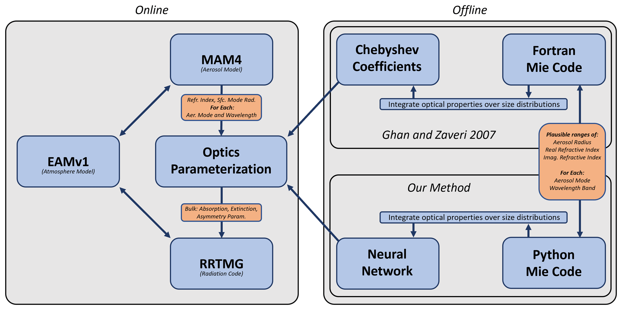
Figure 1A diagram of the aerosol optics parameterization and how it integrates with EAM. The “online” section shows how the parameterization is used during a simulation, and the “offline” portion shows the process of precomputing optical properties and preparing the parameterization.
Errors are introduced at nearly every step in this process, including averaging of within-mode refractive properties, a limited number of wavelength bands treated by the model, assumed aerosol size distributions, interpolation of refractive indices and particle size distributions, and others. This approximation of well understood but unresolvable physics is a frustrating but unavoidable facet of climate modeling. Here, we set out to replace the Chebyshev interpolation approach with a neural network emulator, which addresses the errors incurred by coarsely resolving n, κ, rs, and particle radius information (evaluated in more detail in Table 1 in Sect. 5).
3.1 Mie code
Training a neural network to emulate Mie scattering first required the generation of large training, validation, and testing datasets using established Mie solvers. We chose to refactor the Fortran code used to generate the existing parameterization's precomputed optical properties into Python. The FORTRAN 77 “MIEV0” Mie scattering code (Wiscombe, 1979, 1980a), which was originally used to perform Mie calculations to generate the current EAM parameterization, was replaced by PyMieScatt (Sumlin et al., 2018; Sumlin, 2017), a Python-based Mie code. The machine learning libraries used in this study are also written in Python, and this refactoring allowed for an end-to-end Python-based pipeline for creating the neural network emulator and will enable easier and more flexible editing if new training data need to be generated in the future. Furthermore, PyMieScatt has support for additional scattering models, such as core–shell optics, which we intend to integrate into the neural network emulator in the future. We have made all of the code written for this study available on the project's GitHub repository (see the “Code and data availability” statement).
To ensure that using PyMieScatt did not introduce any additional errors or discrepancy with the original parameterization, we performed a comparison to MIEV0. The optical properties of every refractive index, particle size, and wavelength combination used by the original parameterization were output and compared to the same optical properties computed using PyMieScatt. The maximum, 99.9th-percentile, and 99th-percentile absolute errors are shown in Table A1. Even the most extreme discrepancies between the two schemes are negligible compared with other sources of error in the parameterization.
3.2 Training and validation data
For ANN training, we generated a large table of bulk aerosol optical properties similar to what is described in Sect. 2.3 but with significantly higher resolution in terms of its input variables. We used the same bounds for possible real and imaginary refractive index values, particle radii, and surface mode radius as in Ghan and Zaveri (2007) and also similarly used logarithmic vs. linear spacing depending on the variable (the same wavelength bands and aerosol modes were used). The resolution of each of these variables was increased to 2049 particle radii, 257 mode radii, 129 imaginary refractive indices, and 129 real refractive indices; this is in comparison to 200, 30, 10, and 7 respective values in the original parameterization. The resulting high-resolution table has about 20 000 times the number of entries, takes on the order of 1 d to compute using parallelized calls to PyMieScatt on a modern CPU, and occupies several gigabytes of RAM, making it inappropriate for direct use in an ESM.
When training a neural network, it is best practice to evaluate the ANN on a holdout set of validation data after it is trained as a check for overfitting to the training data. The validation data used here were drawn randomly from the high-resolution table using half of the data points for training and half for validation. In this application, the boundaries of the optical property tables were chosen by Ghan and Zaveri (2007) to encompass all possible input values the parameterization could receive from the ESM, so we are not concerned about poor performance when extrapolating outside of the optics table. However, there is potential for overfitting to cause unexpected behavior in the regions between points in the training set, and this choice of validation set allows for detection of this type of overfit if it occurs.
3.3 Testing data
In addition to a validation set, when hyperparameter tuning is used or multiple models are tested, an additional set of “test” data should be held out to ensure that the validation set has not been overfit by the hyperparameter or model selection (Murphy, 2012). The test set used in this study was generated separately from the training data and is approximately the same size as the combined training and validation sets. The training set was constructed by generating an additional table of optical properties where each of the input parameters bisects the grid of values used to generate the training and validation data. This ensures that it completely covers the range of possible inputs and does not contain values near any of the training and validation data points. This test set was used to ensure that the randomly wired ANN approach did not lead to an overfit of the validation set.
3.4 Benchmark datasets
In addition to the high-resolution optics data used for training and validation, three other tables of optical properties were generated at intermediate resolutions of , , and . Where the table dimensions have been listed in the following order: particle radii × mode radii × imaginary refractive index × real refractive index. We have chosen to scale dimensions to a power of 2 plus 1 so that grid points in a table will be bisected by grid points in the next-highest-resolution table. These datasets have total parameter counts of approximately 108, 107, and 106, respectively, once the multiple wavelengths, aerosol modes, and output parameters are accounted for. Note that the number of particle radii used to resolve the particle size distributions does not add to the size of the optics table and is only used when the dataset is generated, but it is important to the table's accuracy. The total parameter count, in the shortwave table, for example, is computed as follows: number of mode radii × number of imaginary refractive indices × number of real refractive indices × 14 shortwave bands × 4 aerosol modes × 3 optical properties. These additional optics tables were evaluated by linearly interpolating their entries to query points in the test set described above, and the resulting errors are shown in Table 1 in Sect. 5. They provide an indication of how the resolution of the training data might impact the accuracy of the trained neural network parameterization.
3.5 Neural network inputs and outputs
To compute the bulk optical properties of a population of homogeneous spheres with lognormally distributed radii, five values must be known: the real and imaginary components of the refractive index, the geometric mean radius and log-standard deviation that define the size distribution, and the wavelength of light. For the parameterization problem solved here, we assist the neural network by encoding this information in a format more conducive to training neural networks.
Neural networks tend to perform better when input and output data have certain well-behaved distributions and formats. Several pre- and post-processing steps were used alongside the ANN to help ensure optimal performance. Each ANN has nine inputs (in order): λ, n, κ, , rs, and a “one-hot” encoding of the four aerosol modes (four values). The one-hot encoding is a common strategy for categorical inputs and usually leads to better performance than a single scalar input that encodes the category (Murphy, 2012, p. 35). The existing parameterization prescribes a log-standard deviation for each aerosol mode, so the log-standard deviation was not included as a separate continuous input. We chose to include as a constructed input despite the fact that both of these variables are used as individual inputs because the size parameter is a key input for Mie scattering calculations, and we found this to improve model skill in early experiments. All of the inputs other than the one-hot encoding are scalar and are each standardized by first taking the log (except for real refractive indices where a log is not used) and then subtracting the mean and dividing by the standard deviation (each rounded to a precision of 0.1). The means and standard deviations used are shown in Table A2 and are based on data from the training set. This yields dimensionless, zero-centered inputs with a standard deviation of 1 and without extreme skew or leptokurtosis.
The Ghan and Zaveri (2007) parameterization estimates specific extinction, absorption, and scattering efficiencies, which are bulk optical properties of the aerosol distribution per total wet aerosol mass, but these values can span several orders of magnitude and, thus, are not well suited for prediction with a neural network. Instead, we have the neural network estimate a key intermediate value used in the Ghan and Zaveri (2007) parameterization that encapsulates the computationally expensive components of estimating bulk aerosol optical properties:
where σ is the log-standard deviation of the particle size distribution, r is wet particle radius, λ is wavelength, m is the complex refractive index, Q is either the extinction or absorption efficiency (see Ghan and Zaveri, 2007, their Eq. 20), and the overline indicates a bulk optical property. In MAM, the values of σ are prescribed for each mode: 1.6 for modes 2 and 4 and 1.8 for modes 1 and 3.
While the values of Eq. (1) are constrained to a reasonable range, linear scaling of the outputs of the ANN is still used to ensure that they are bounded by zero and one. This allows the use of a sigmoid output function to constrain the ANN's outputs. The bulk absorption efficiency is linearly scaled by a factor of 2.2, whereas the bulk extinction efficiency is scaled by 4.6. These values were determined empirically from the training set; when the parameterization is used in an ESM, this scaling will need to be applied. The bulk asymmetry parameter () is naturally bounded by zero to one for the range of inputs in this study and is not scaled (Bohren and Huffman, 1983). The longwave and shortwave bands have significantly different ranges for some of their inputs, and the existing parameterization only computes bulk absorption in the longwave, so two neural networks were trained: one with three outputs to process the shortwave bands and one with a single output to process the longwave bands.
4.1 Neural architecture search
Neural networks are powerful data-fitting tools, and simple ANN designs can easily generalize to a wide variety of problems. Even so, specialized ANN architectures that have been optimized for a task will usually perform best. Task-specific ANN design is difficult, however, because the space of reasonable ANN designs is usually far too large to explore exhaustively, and it is not usually obvious which will work best. Typically, researchers will rely on heuristics, past experience, or simply convenience and popularity to choose an appropriate ANN architecture.
Various algorithmic approaches to neural architecture search (NAS) (Elsken et al., 2019) and hyper-parameter optimization (HPO) (Feurer and Hutter, 2019) have become popular for addressing this problem. These algorithms usually involve training many different neural networks with a range of parameter and design choices and selecting the best-performing models. Search methods range from simple random or grid search to sophisticated algorithms such as evolutionary optimization (Angeline et al., 1994), Bayesian optimization (Bergstra et al., 2013), or reinforcement learning (Baker et al., 2017). Much of the recent (past 10 years) research in neural architecture search has focused on developing new convolutional neural network architectures for image processing (e.g., Zoph et al., 2018). Elsken et al. (2019) and Yao (1999) provide reviews of this topic.
Most NAS strategies that test a variety of network wiring patterns are limited to exploring certain families of predefined network styles or break up the search space by randomizing individual network “cells” that are then wired together in sequence. However, Xie et al. (2019) demonstrated a NAS strategy in which new convolutional neural network architectures were discovered through random wiring of network layers. Motivated by early observations during our work that the inclusion of skip connections and more complex wirings contributed to performance for the aerosol optics problem, we chose to employ a similar approach here. Whereas Xie et al. (2019) focus on convolutional neural networks, we use ANNs constructed of fully connected layers. In general, skip connections and complex wirings are much more common in deep convolutional neural network architectures than ones constructed from fully connected layers, but there is some past evidence that including skip connections in deep fully connected networks can improve performance on certain non-linear problems (Lang and Witbrock, 1988), and this seems to be the case for the problem of emulating Mie scattering. Here, we designed an ANN generator that automatically produces ANNs with a random number of layers, random layer sizes, and random connections between layers. Ultimately the randomly generated wirings allow for the discovery of networks that substantially outperform simple multilayer perceptrons.
4.2 Random network motivation
The physical parameterization problem discussed in this paper is particularly well suited for an ANN. The bulk aerosol optical properties used by the parameterization can be thought of as smooth, bounded, manifolds in a high-dimensional space, and representing this type of dataset is an area where neural networks often excel. It is also a particularly data-rich problem because the only limits to the size of our training dataset are the computational and storage resources that we would like to devote to generating training data (and ultimately an upper bound on training set resolution where neighboring data points become highly autocorrelated). In early experiments, we found that while simple feed-forward multilayer-perceptron-style architectures with one to two hidden layers can provide much higher performance than the current EAMv1 parameterization discussed in Sect. 2.3, more complex architectures that included many smaller layers with skip connections could achieve even higher accuracy without an increase in the number of model parameters. Ultimately, when used in a climate model, the ANN-based parameterization will be evaluated many times (every time the radiative transfer code is called for each model grid cell). This means that reducing the network size as much as possible without significantly reducing accuracy is a worthwhile endeavor and can save both computation time and memory when the climate model is run. Additionally, because of the relatively small size (500–100 000 parameters) of the ANNs used here, they are cost-effective to train. Together, these factors mean that this ML problem is ideal for NAS.
4.3 The random ANN generator
Our ANN generator randomizes the network layer size, layer count, merge operators, and wiring. First, it randomly chooses a number of layers between 2 and 12; it then randomly chooses the number of neurons per layer by choosing an integer between 7 and 45 and scaling it by a factor of 0.5Nlayers (the scaling prevents the generation of very deep and wide ANNs with extremely high parameter counts). To facilitate merging inbound tensors to a layer with element-wise addition, all layers in the network use the same number of neurons. Each hidden layer used in the network is a fully connected layer and applies a tanh activation to its outputs.
Once layer counts and size are selected, the ANN generator creates a random wiring between the layers by generating an adjacency matrix that represents layer connections. Several constraints must be enforced on the adjacency matrix to ensure that it represents a usable ANN architecture. Firstly, we require that the ANN is feed forward. If each row in the adjacency matrix represents a layer in the order in which they will be evaluated in the ANN, this can be accomplished by enforcing that the adjacency matrix is lower triangular. For an ANN with N hidden layers, this means there are valid layer connections. The number of active connections for an ANN is randomly chosen from a uniform distribution between 0 and , and this many entries in the lower triangular portion of the adjacency matrix are then randomly turned on. Additionally, each layer must have at least one inbound and one outbound tensor. Because the number of layers in the ANN is determined before the adjacency matrix is constructed, this must be enforced by iterating through each row and column of the adjacency matrix and randomly turning on one valid inbound and/or outbound connection if the corresponding layer has none.
Lastly, the number of inputs to each ANN are static (nine inputs), but we would like the outputs from each network layer to be a fixed size, and any layer can be directly connected to the input layer. As a workaround, each ANN includes an additional fully connected layer with a number of neurons equal to the difference between the nine inputs and the randomly selected network layer size. The outputs from this layer are appended to the actual inputs as a learnable padding.
Initial experiments on a subset of the training data were run using a single shortwave band (because of reduced training time on the smaller dataset) with additional randomization including the following: variable layer sizes (ANNs that used different layer sizes internally exclusively used concatenation to merge tensors); randomly selected activation functions from linear, tanh, rectified linear unit (ReLU) (Glorot et al., 2011), exponential linear unit (Clevert et al., 2015), leaky ReLU, and parametric ReLU (He et al., 2015); and batch normalization (Ioffe and Szegedy, 2015), dropout (Srivastava et al., 2014), or no regularizer. These experiments showed that the tanh function provided slightly better performance than other activations and that including batch normalization or dropout substantially reduced performance. We hypothesize that the reduced performance with dropout is related to the fact that we are testing relatively small networks. Because dropout layers generally force the ANNs to learn redundant representations of the data and the small ANNs used here only have limited capacity to represent the complex training data, requiring them to learn redundant representations of the data only reduces their skill. Additionally, the complexity of the training data and small size of the networks means that we are not particularly concerned about overfitting and do not expect to gain much from using regularization techniques. These additional types of randomization were not included in final experiments.
4.4 Training and model selection
Each model was trained using the Adam optimizer with an initial learning rate of 0.001, β1=0.9, and β2=0.999 to optimize mean-squared error. We used a batch size of 64 samples and trained for 10 epochs. The learning rate was reduced manually by a factor of 10 on the 4th, 7th, and 10th epochs. A total of 500 randomly wired ANNs were trained, and each was evaluated on the validation set. Figure 2 shows scatterplots of each random ANN's validation performance in terms of mean absolute error (MAE) on the standardized ANN outputs plotted against the number of trainable parameters in the network. Both panels in Fig. 2 show a similar pattern in terms of ANN performance vs. size: skill improves rapidly with increasing size until it plateaus somewhere between 1000 and 20 000 trainable parameters. Additional size increases yield only very small performance gains. The approximate location of the elbow in each of these performance vs. size plots is expanded in an inset in each figure panel. Based on these inset plots, we subjectively chose an ANN for both the longwave and shortwave regimes that appears to provide a good balance between network size and skill. The selected ANNs are denoted in Fig. 2 with red circles, and diagrams of the wirings for the selected networks are shown in Fig. 3. Note that later, in Sect. 5, errors will be reported after rescaling the standardized network outputs for comparison to the Ghan and Zaveri (2007) scheme; however, here, we report the selected ANNs' MAEs on the test set computed directly on the ANN output as in Fig. 2: shortwave (SW): ; longwave (LW): . The comparable performance on the test set to the validation set indicates that the chosen ANNs did not overfit the training and validation data. These selected ANNs were ultimately retained for use as parameterizations and are evaluated in more detail on the test set in Sect. 5.
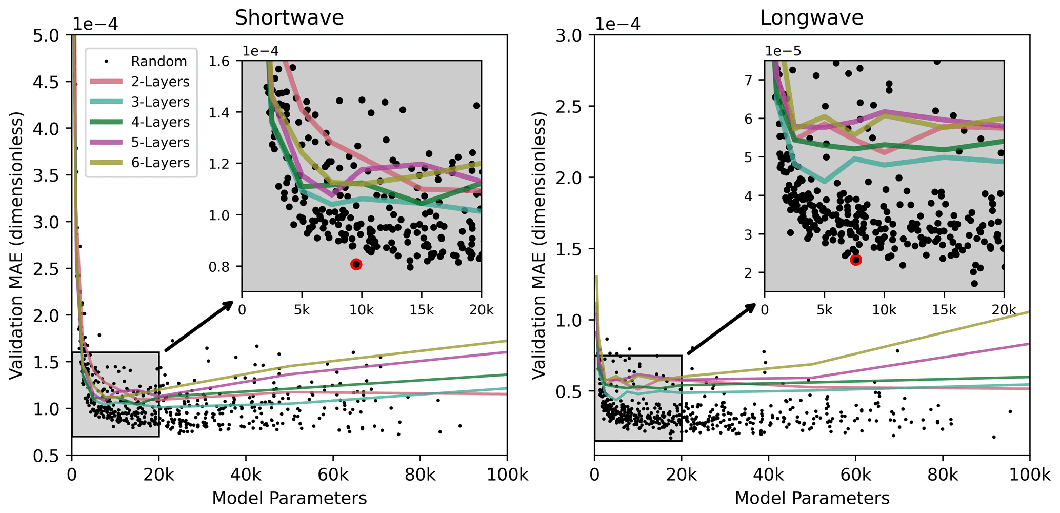
Figure 2Validation set performance of randomly wired neural networks plotted against the network size. Panels show results for different wavelength regimes. The mean absolute error is computed on normalized optical properties (directly on the outputs from the neural networks) and are dimensionless. In each case, there is a clear elbow, beyond which increasing the network size does not substantially improve performance. In both panels, the inset shows a magnified region around this elbow. Solid lines indicate the performance of traditional feed-forward multilayer perceptron ANNs with two to six hidden layers. The red dot indicates the network that was ultimately chosen for use.
We also trained several benchmark ANNs for comparison to the random ANNs. Each of the benchmark networks is composed of two to six hidden layers wired in sequence with tanh activation functions, and they represent the performance of conventional ANN architectures. One-layer ANNs performed almost an order of magnitude worse than the others and were not included. Benchmark ANNs with a total of 10 different sizes in terms of total trainable parameters were used. Five copies of each unique benchmark ANN layer count–parameter count combination were trained, and only the best-performing models were retained to ensure that poor performance at a particular ANN size was not simply due to an unlucky random initialization or training sample selection. This means that a total of 250 benchmark ANNs were trained for both the longwave and shortwave regimes. The performance of these benchmark ANNs is also indicated in Fig. 2 by solid lines.
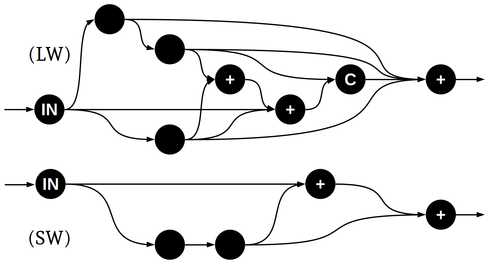
Figure 3Wiring patterns of the two (longwave and shortwave) randomly generated neural networks that were selected for use in the optics emulator. Nodes represent “dense” (fully connected) layers. “C” and “+” indicate whether inbound tensors are combined by concatenation or addition, respectively. All hidden layers have the same number of neurons within each network: SW has 54 and LW has 32 (the nine inputs are padded to reach the appropriate size, and the output layer has either 3 neurons for SW or 1 neuron for LW).
4.5 Discussion of ANN architecture
The performance of the benchmark and random ANNs provides some insight into ANN design. Firstly, we note that one-layer ANNs were also tested, but they typically performed nearly an order of magnitude worse than other ANNs and are not shown in Fig. 2. This suggests that using almost any multilayer architecture, regardless of construction, can yield substantial performance gains. Secondly, the two- to six-layer sequential models are outperformed by the majority of randomly wired ANNs that have similar parameter counts. Also, the multilayer sequential models with more than three layers begin to perform worse than their shallower counterparts. It appears that the inclusion of skip connections has likely allowed the random networks to train successfully despite their depth (high layer count). In the context of this problem, the neural networks are attempting to fit a high-dimensional manifold that varies significantly with respect to several of the input parameters. Deeper networks are likely required to efficiently represent the non-linearities in the problem, but deep neural networks can struggle to train effectively due to vanishing gradients (Goodfellow et al., 2016). The ANNs that were ultimately chosen here tend to have more, but smaller, layers than the best serially connected ANNs, and they include multiple skip connections.
The universal approximation theorem implies that this problem is solvable with a wide, single-layer perceptron network (Hornik et al., 1989). In practice, however, multilayer networks are almost always more efficient, and this is the case here. Furthermore, any of the randomly wired networks used here could theoretically be represented by a serially connected multilayer network: one can imagine a serially connected network learning to apply the identity function to some of its inputs, thereby learning to generate skip connections on its own. Again, while it is technically possible, this is not the case in practice, and even learning the identity function is not necessarily a trivial task for neural networks. While the importance of skip connections has been thoroughly explored in the context of building very deep convolutional neural networks (He et al., 2016), it has only rarely been applied to ANNs with fully connected layers, although some early examples of this approach do exist (Lang and Witbrock, 1988). These results are informative for our application and similar use cases, where the ANN's memory and computational requirements at the inference time are of particular importance; moreover, by evaluating many ANN architectures, we have identified ANNs with significantly higher accuracy than conventional architectures with no increase in inference cost. Taken together, our results indicate that significant performance gains may be achieved in other applications of ANNs in the Earth sciences and Earth system modeling through in-depth exploration of task-optimized network architectures.
The ANNs were ultimately evaluated on the randomly generated holdout test set described in Sect. 3.3. In addition to evaluating the accuracy of their outputs, we evaluate them on two additional optical properties derived from the ANN output: shortwave bulk scattering efficiency () and single-scattering albedo (SSA). These respective properties are computed as follows: and (Bohren and Huffman, 1983). SSAs with were not included in the analysis because very small errors get amplified by the in scenarios where scattering is negligible. The existing aerosol optics parameterization was also evaluated along with linear interpolation applied to several high-resolution tables of aerosol optical properties that were generated at a range of resolutions (described in Sect. 3.4). This includes the very high resolution table used for training and validation. The test set MAE for each of the output parameters and wavelength regimes are listed in Table 1. The ANN shows a substantial performance improvement over the existing parameterization, with MAEs about 3 orders of magnitude smaller. This is particularly notable for the shortwave extinction efficiencies where the existing parameterization has an MAE of 0.2 but the ANN has an MAE of . Extinction efficiencies range from about 0 to 3.5, so an MAE of 0.2 is substantial. The performance of the additional interpolated optics tables behaves about as expected, with the MAE decreasing in proportion to table size. It can also be seen that a lookup table with approximately 109 parameters is required to achieve performance comparable to the ANN. This is far too large to be used in an ESM. Lastly, Table 1 indicates the test set performance of the best-performing conventional (serially connected) ANN on the test set, and again we see that it cannot match the performance of the randomly wired ANN, which consistently outperforms it by around 10 % to 30 % for the shortwave and 65 % for the longwave.
Ghan and Zaveri (2007)Table 1Mean absolute error for bulk optical property estimates using different methods. Note that only bulk absorption efficiency is computed for the longwave bands and that shortwave single-scattering albedo (SSA) and bulk scattering efficiency are computed from shortwave absorption and extinction efficiencies. The overbars denote that these are bulk values integrated over lognormal size distributions (Eq. 1).
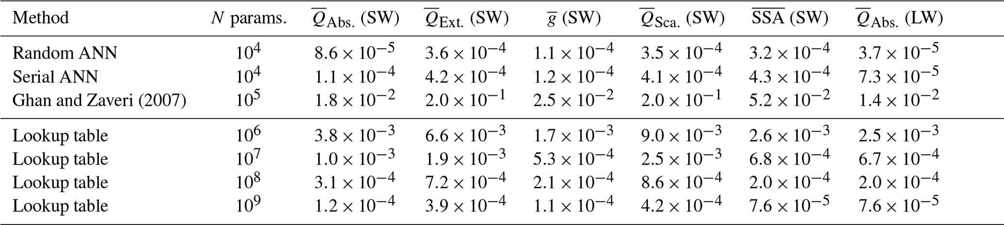

Figure 4Error histograms for estimates of the bulk aerosol optics test dataset. These panels show the distribution of errors on a log–log histogram to make outlier cases with high error more apparent. The vertical grid shows the bin edges of the histogram. The blue and magenta lines represent the Chebyshev-polynomial-based parameterization and the neural network, respectively. The dashed gray lines represent the error from applying linear interpolation to precomputed optics datasets of varying resolution, with the highest-resolution tables appearing to the left and progressively coarser tables to the right.
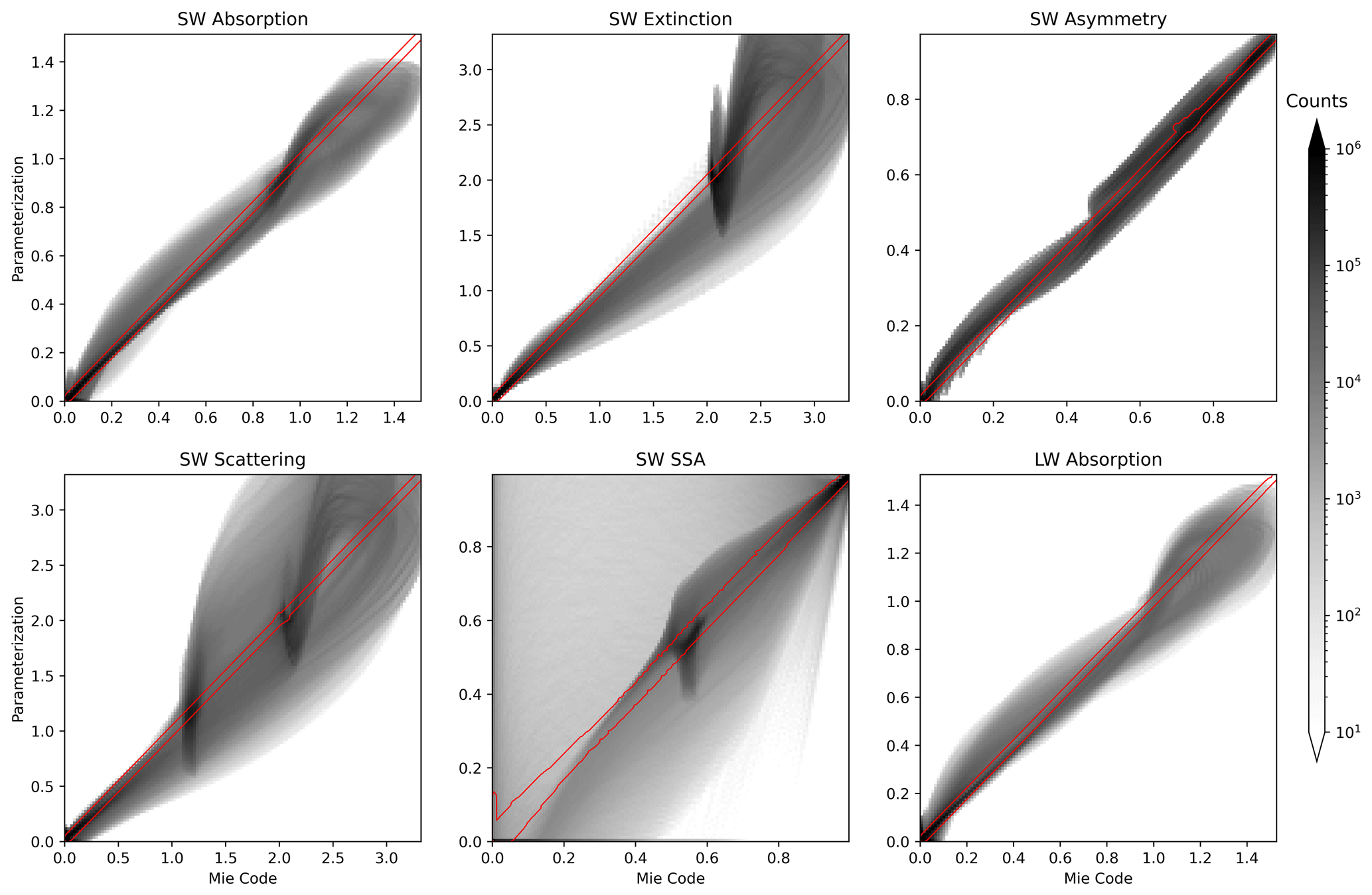
Figure 5Scatterplot-like joint histograms comparing optical properties from the Chebyshev-interpolation-based parameterization and Mie code. Gray shading indicates the density of data points. The red contour contains all outputs from the neural network, which all lie very close to the 1-to-1 line.
The very low MAE shown in Table 1 is encouraging, but ideally a parameterization should perform well over the full range of possible inputs and a low MAE could potentially still be achieved in the presence of outlier cases with high error that could cause problems when it is used in a climate simulation. Figure 4 shows logarithmically scaled histograms of the absolute error for all individual samples in the test set. Here, we see that, in addition to outperforming the benchmark optics tables and existing parameterization on average, the most extreme errors produced by the ANN are also far smaller than those produced by the existing parameterization. Furthermore, the ANN's histograms tend to have peaks at lower error values than the other methods. Note that, because of the log scaling, the peak represents a large number of samples and the size of the error distribution's tails is exaggerated. An interesting feature from Fig. 4 is that the lookup tables tend to have longer left tails, representing cases with very low error. These occur because some regions in the input space have little to no variability in the output space – for instance, the large regions where extinction is near zero. The linear interpolation in the lookup tables can perfectly fit constant-valued functions, but the ANN and Chebyshev methods will still have a small amount of error. Ultimately, the key observation from Fig. 4 is that the ANN's errors do not have a large right tail, meaning that we still expect very accurate estimates of aerosol optical properties, even for the input queries where the ANN performs worst.
Finally, Fig. 5 shows a joint histogram of bulk aerosol optical properties estimated by the existing parameterization and by direct computation with Mie code for all samples in the test set. Separate joint histograms are not included for the ANN outputs; instead, a red contour in each of the joint histograms denotes the boundary containing all samples. Notable patterns appear in the joint histograms of the shortwave extinction field and the fields derived from it (SW scattering and SSA) as well as, to a lesser degree, the other predicted fields. These arise in the Ghan and Zaveri (2007) parameterization from the Chebyshev polynomial fit used to approximate optical properties as a function of surface mode radius. The Chebyshev polynomials are smooth functions that do not perfectly fit the bulk extinction efficiency curve, for instance, and consistently over- or undershoot it for certain rs values. Because bulk extinction efficiency is very sensitive to the particle size distribution, this effect is obvious in Fig. 5.
Drawing the training set from a regular grid over the input space has ensured good coverage of possible input values, while generating a test set of equal size consisting of intermediate values that are not near points in the training or validation data helps demonstrate that the ANN will not perform unexpectedly when interpolating within the region defined by the training data. Together, Table 1 and Figs. 4 and 5 demonstrate that the ANN parameterization not only provides a dramatic performance improvement over the current approach but can also be expected to perform exceedingly well for the full range of possible input data, with no extreme cases of high error. Therefore, the ANN parameterization is an accurate and reliable replacement for the current bulk aerosol optics parameterization.
This work has demonstrated the effectiveness of machine learning for emulating the aerosol optical properties that are crucial to climate simulation. A neural network is capable of producing bulk optical property estimates that are substantially more accurate than those produced by the existing (Ghan and Zaveri, 2007) parameterization in E3SM and CESM and does so with an order of magnitude smaller memory requirement. The computational requirements for evaluating an ANN with 104 parameters is larger than the computational requirements of the current approach, but this parameterization is evaluated every time EAM calls radiation code, and evaluating the ANN requires negligible computation compared with the radiation code, so the impact on model runtime should be negligible. Additionally, the ANN outperforms lookup-table-based optics emulators that resolve aerosol optical properties at much higher resolution than the existing scheme. Testing over a wide range of possible input data showed that the neural network performs well over the possible input space and will not produce any outlier errors or unexpected results within this range. Representation of aerosol direct effects is a major source of uncertainty in climate simulation; while representation of aerosol optics is likely only a small component of this uncertainty, adequate representation of these physics is a key step forward towards accurately representing aerosols in general.
This work, to some degree, should be seen as a first step or proof of concept and as a demonstration of the power of randomly wired networks for this problem. Our ultimate goal is to develop a neural-network-based parameterization that represents core–shell scattering – a physical model that is too computationally expensive to represent with existing parameterizations. While this work presents the machine learning technique and evaluates it directly against Mie code, we expect to follow it with a climate modeling study evaluating the impacts of this parameterization, and a future core–shell scattering model, on E3SM simulations.
In addition to developing a new parameterization, we applied a recently developed (Xie et al., 2019) neural architecture search strategy that randomizes wiring patterns in deep neural networks. Key findings were that deeper ANNs significantly outperformed a single-layer ANN of comparable size. Also, the majority of randomly constructed ANN architectures (which include skip connections) outperformed conventional multilayer perceptron networks. In the context of this study, the NAS allowed us to identify neural architectures that provide a substantial performance improvement with no increase in network size.
Our findings provide some insights into ANN design. The fact that the majority of randomly wired networks outperform multilayer networks with serially connected layers indicates that the inclusion of skip connections may be critical for this type of problem. In image processing, convolutional neural networks with a large number of layers and skip connections (He et al., 2016; Huang et al., 2017) were identified as superior to serially connected designs several years ago, and they have dominated deep learning research since. While using skip connections in networks constructed of fully connected layers is certainly not a new idea (Lang and Witbrock, 1988), it has received comparatively little attention in recent machine learning literature. This work indicates that the inclusion of skip connections could be an effective way to train smaller regressor and function-fitting neural networks to fit complicated data or surfaces.
To the best of our knowledge, this is the first use of randomly wired neural architecture search approaches in the atmospheric sciences. Their performance against conventional serially connected feed-forward ANNs in this task was striking. The majority of random wirings were better able to represent Mie optics than serial wirings by a substantial amount (about 10 %–30 % in the shortwave regime and 65 % in the longwave) with no increase in model complexity in terms of the number of trainable parameters. There has recently been significant push to leverage new advances in machine learning to replace the various existing parameterizations used by climate and weather models with more performant and/or accurate representations (e.g., Gettelman et al., 2021; Lagerquist et al., 2021). Many of these problems, like the Mie optics problem addressed here, are data-rich and well suited for neural architecture search, as training data can be produced by an accurate but computationally expensive numerical simulation. Our results indicate that, when using neural networks for this type of application, significant performance improvements can be achieved by taking care to design or select network architectures optimized for the target task. NAS algorithms and random wirings have, so far, received little attention in the Earth sciences, and random network wiring may be a fruitful strategy for developing neural-network-based parameterizations and physics emulators in the future.
Table A1Errors between optical properties computed with PyMieScatt and MIEV0.
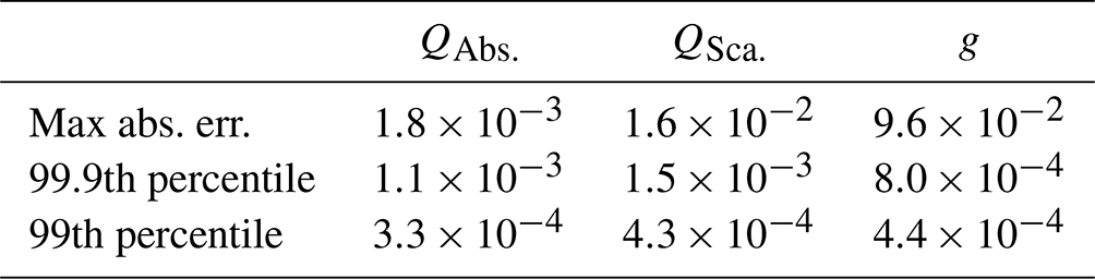
Table A2Constants used to standardize ANN inputs. For all variables except the real refractive index, standardization is done after taking the natural logarithm. A value of is added to the imaginary refractive index before taking the logarithm.

The code created as part of this research is available from the project's GitHub repository (https://github.com/avgeiss/aerosol_optics_ml, last access: 20 February 2023) and has been archived on Zenodo: https://doi.org/10.5281/zenodo.6767169 (Geiss, 2022a).
Wiscombe's MIEV0 is thoroughly documented in Wiscombe (1979, 1980a) and has been preserved in several locations online, including as part of the CESM 1.0 code: https://www.cesm.ucar.edu/models/cesm1.0/cesm/cesmBbrowser/html_code/cam/miesubs.F.html##MIEV0 (last access: 25 April 2022) and https://github.com/avgeiss/aerosol_optics_ml/blob/main/mie_codes/miev0.F (Wiscombe, 1980b).
PyMieScatt is available from https://github.com/bsumlin/PyMieScatt (Sumlin, 2017) and can be installed via the pip Python package manager. PyMieScatt documentation is available from https://pymiescatt.readthedocs.io/en/latest/ (last access: 8 February 2022).
All data produced as part of this study, including optics tables, random ANN files, and Chebyshev coefficients generated by our Python port of the Ghan and Zaveri (2007) parameterization, have been made available online at https://doi.org/10.5281/zenodo.6762700 (Geiss, 2022a). We note that all of the data stored here can be produced by running the code in the project's GitHub repository.
AG wrote the manuscript, performed the experiments, and developed the methods and code. PLM secured funding, conceived the project, edited the manuscript, and provided assistance with Fortran code. JCH provided input on project planning and direction. BS provided assistance with the Fortran code.
At least one of the (co-)authors is a member of the editorial board of Geoscientific Model Development. The peer-review process was guided by an independent editor, and the authors also have no other competing interests to declare.
Publisher's note: Copernicus Publications remains neutral with regard to jurisdictional claims in published maps and institutional affiliations.
The research used high-performance computing resources from PNNL Research Computing as well as resources from the National Energy Research Scientific Computing Center (NERSC), a U.S. Department of Energy Office of Science User Facility located at Lawrence Berkeley National Laboratory (operated under contract no. DE-AC02-05CH11231 using NERSC award nos. ALCC-ERCAP0016315, BER-ERCAP0015329, BER-ERCAP0018473, and BER-ERCAP0020990). We would also like to thank Sam J. Silva and William Yik for their helpful discussions regarding randomly wired neural networks.
This study was supported as part of the “Enabling Aerosol–cloud interactions at GLobal convection-permitting scalES (EAGLES)” project (project no. 74358), sponsored by the U.S. Department of Energy, Office of Science, Office of Biological and Environmental Research, Earth System Model Development (ESMD) program area. The Pacific Northwest National Laboratory is operated for DOE by Battelle Memorial Institute under contract DE-AC05-76RL01830.
This paper was edited by Samuel Remy and reviewed by two anonymous referees.
Albrecht, B. A.: Aerosols, cloud microphysics, and fractional cloudiness, Science, 245, 1227–1230, 1989. a
Angeline, P., Saunders, G., and Pollack, J.: An evolutionary algorithm that constructs recurrent neural networks, IEEE T. Neural Networ., 5, 54–65, https://doi.org/10.1109/72.265960, 1994. a
Baker, B., Gupta, O., Naik, N., and Raskar, R.: Designing Neural Network Architectures using Reinforcement Learning, ArXiv [preprint], https://doi.org/10.48550/arXiv.1611.02167, 2017. a
Bellouin, N., Quaas, J., Gryspeerdt, E., Kinne, S., Stier, P., Watson-Parris, D., Boucher, O., Carslaw, K. S., Christensen, M., Daniau, A.-L., Dufresne, J.-L., Feingold, G., Fiedler, S., Forster, P., Gettelman, A., Haywood, J. M., Lohmann, U., Malavelle, F., Mauritsen, T., McCoy, D. T., Myhre, G., Mülmenstädt, J., Neubauer, D., Possner, A., Rugenstein, M., Sato, Y., Schulz, M., Schwartz, S. E., Sourdeval, O., Storelvmo, T., Toll, V., Winker, D., and Stevens, B.: Bounding global aerosol radiative forcing of climate change, Rev. Geophys., 58, e2019RG000660, https://doi.org/10.1029/2019RG000660, 2020. a, b
Bergstra, J., Yamins, D., and Cox, D.: Making a Science of Model Search: Hyperparameter Optimization in Hundreds of Dimensions for Vision Architectures, in: Proceedings of the 30th International Conference on Machine Learning, edited by: Dasgupta, S. and McAllester, D., Proceedings of Machine Learning Research, Atlanta, Georgia, USA, Vol. 28, 115–123, https://doi.org/10.5555/3042817.3042832, 2013. a
Bohren, C. F. and Huffman, D. R.: Absorption and Scattering of Light by Small Particles, John Wiley and Sons Inc., ISBN 0-471-05772-X, 1983. a, b, c, d
Boucher, O., Randall, D., Artaxo, P., Bretherton, C., Feingold, G., Forster, P., Kerminen, V.-M., Kondo, Y., Liao, H., Lohmann, U., Rasch, P., Satheesh, S., Sherwood, S., Stevens, B., and Zhang, X.: Clouds and Aerosols. In: Climate Change 2013: The Physical Science Basis, Contribution of Working Group I to the Fifth Assessment Report of the Intergovernmental Panel on Climate Change, Cambridge University Press, Cambridge, United Kingdom and New York, NY, USA, https://doi.org/10.1017/CBO9781107415324.016, 2013. a
Boukabara, S.-A., Krasnopolsky, V., Penny, S. G., Stewart, J. Q., McGovern, A., Hall, D., Ten Hoeve, J. E., Hickey, J., Huang, H.-L. A., Williams, J. K., Ide, K., Tissot, P., Haupt, S. E., Casey, K. S., Oza, N., Geer, A. J., Maddy, E. S., and Hoffman, R. N.: Outlook for exploiting artificial intelligence in the earth and environmental sciences, B. Am. Meteorol. Soc., 102, E1016–E1032, 2021. a
Brenowitz, N. D. and Bretherton, C. S.: Prognostic validation of a neural network unified physics parameterization, Geophys. Res. Lett., 45, 6289–6298, 2018. a
Bretherton, C. S., Henn, B., Kwa, A., Brenowitz, N. D., Watt-Meyer, O., McGibbon, J., Perkins, W. A., Clark, S. K., and Harris, L.: Correcting Coarse-Grid Weather and Climate Models by Machine Learning From Global Storm-Resolving Simulations, J. Adv. Model. Earth Sy., 14, e2021MS002794, https://doi.org/10.1029/2021MS002794, 2022. a
Clevert, D.-A., Unterthiner, T., and Hochreiter, S.: Fast and accurate deep network learning by exponential linear units (elus), arXiv [preprint], https://doi.org/10.48550/arXiv.1511.07289, 2015. a
Danabasoglu, G., Lamarque, J.-F., Bacmeister, J., Bailey, D. A., DuVivier, A. K., Edwards, J., Emmons, L. K., Fasullo, J., Garcia, R., Gettelman, A., Hannay, C., Holland, M. M., Large, W. G., Lauritzen, P. H., Lawrence, D. M., Lenaerts, J. T. M., Lindsay, K., Lipscomb, W. H., Mills, M. J., Neale, R., Oleson, K. W., Otto-Bliesner, B., Phillips, A. S., Sacks, W., Tilmes, S., van Kampenhout, L., Vertenstein, M., Bertini, A., Dennis, J., Deser, C., Fischer, C., Fox-Kemper, B., Kay, J. E., Kinnison, D., Kushner, P. J., Larson, V. E., Long, M. C., Mickelson, S., Moore, J. K., Nienhouse, E., Polvani, L., Rasch, P. J., and Strand, W. G.: The community earth system model version 2 (CESM2), J. Adv. Model. Earth Sy., 12, e2019MS001916, https://doi.org/10.1029/2019MS001916, 2020. a
Elsken, T., Metzen, J. H., and Hutter, F.: Neural Architecture Search: A Survey, J. Mach. Learn. Res., 20, 1–21, http://jmlr.org/papers/v20/18-598.html (last access: 10 February 2023), 2019. a, b
Fan, J., Wang, Y., Rosenfeld, D., and Liu, X.: Review of aerosol–cloud interactions: Mechanisms, significance, and challenges, J. Atmos. Sci., 73, 4221–4252, 2016. a
Friedlander, S. K.: Smoke, Dust, and Haze Fundamentals of Aerosol Dynamics, Topics in chemical engineering, Oxford University Press, New York, NY, ISBN 0-19-512999-7, 2000. a
Geiss, A.: avgeiss/aerosol_optics_ml: GMD Supplementary Code (Version v1), Zenodo [code], https://doi.org/10.5281/zenodo.6767169, 2022a. a
Geiss, A.: Aerosol Optics ML Datasets, Zenodo [data set], https://doi.org/10.5281/zenodo.6762700, 2022b. a
Geiss, A., Silva, S. J., and Hardin, J. C.: Downscaling atmospheric chemistry simulations with physically consistent deep learning, Geosci. Model Dev., 15, 6677–6694, https://doi.org/10.5194/gmd-15-6677-2022, 2022. a
Gelbard, F. and Seinfeld, J. H.: The general dynamic equation for aerosols. Theory and application to aerosol formation and growth, Journal of Colloid and Interface Science, 68, 363–382, https://doi.org/10.1016/0021-9797(79)90289-3, 1979. a
Gelbard, F., Tambour, Y., and Seinfeld, J. H.: Sectional representations for simulating aerosol dynamics, J. Colloid Interf. Sci., 76, 541–556, https://doi.org/10.1016/0021-9797(80)90394-X, 1980. a
Gettelman, A., Gagne, D. J., Chen, C.-C., Christensen, M., Lebo, Z., Morrison, H., and Gantos, G.: Machine learning the warm rain process, J. Adv. Model. Earth Sy., 13, e2020MS002268, https://doi.org/10.1029/2020MS002268, 2021. a, b
Ghan, S., Laulainen, N., Easter, R., Wagener, R., Nemesure, S., Chapman, E., Zhang, Y., and Leung, R.: Evaluation of aerosol direct radiative forcing in MIRAGE, J. Geophys. Res.-Atmos., 106, 5295–5316, 2001. a
Ghan, S. J. and Zaveri, R. A.: Parameterization of optical properties for hydrated internally mixed aerosol, J. Geophys. Res.-Atmos., 112, D10201, https://doi.org/10.1029/2006JD007927, 2007. a, b, c, d, e, f, g, h, i, j, k, l, m, n, o, p
Glorot, X., Bordes, A., and Bengio, Y.: Deep sparse rectifier neural networks, in: Proceedings of the fourteenth international conference on artificial intelligence and statistics, JMLR Workshop and Conference Proceedings, https://proceedings.mlr.press/v15/glorot11a.html (last access: 10 February 2023), 315–323, 2011. a
Golaz, J.-C., Caldwell, P. M., Van Roekel, L. P., Petersen, M. R., Tang, Q., Wolfe, J. D., Abeshu, G., Anantharaj, V., Asay-Davis, X. S., Bader, D. C., Baldwin, S. A., Bisht, G., Bogenschutz, P. A., Branstetter, M., Brunke, M. A., Brus, S. R., Burrows, S. M., Cameron-Smith, P. J., Donahue, A. S., Deakin, M., Easter, R. C., Evans, K. J., Feng, Y., Flanner, M., Foucar, J. G., Fyke, J. G., Griffin, B. M., Hannay, C., Harrop, B. E., Hoffman, M. J., Hunke, E. C., Jacob, R. L., Jacobsen, D. W., Jeffery, N., Jones, P. W., Keen, N. D., Klein, S. A., Larson, V. E., Leung, L. R., Li, H.-Y., Lin, W., Lipscomb, W. H., Ma, P.-L., Mahajan, S., Maltrud, M. E., Mametjanov, A., McClean, J. L., McCoy, R. B., Neale, R. B., Price, S. F., Qian, Y., Rasch, P. J., Reeves Eyre, J. E. J., Riley, W. J., Ringler, T. D., Roberts, A. F., Roesler, E. L., Salinger, A. G., Shaheen, Z., Shi, X., Singh, B., Tang, J., Taylor, M. A., Thornton, P. E., Turner, A. K., Veneziani, M., Wan, H., Wang, H., Wang, S., Williams, D. N., Wolfram, P. J., Worley, P. H., Xie, S., Yang, Y., Yoon, J.-H., Zelinka, M. D., Zender, C. S., Zeng, X., Zhang, C.,Zhang, K., Zhang, Y., Zheng, X., Zhou, T., and Zhu, Q.: The DOE E3SM coupled model version 1: Overview and evaluation at standard resolution, J. Adv. Model. Earth Sy., 11, 2089–2129, 2019. a, b
Goodfellow, I., Bengio, Y., and Courville, A.: Deep Learning, MIT Press, http://www.deeplearningbook.org (last access: 23 June 2022), 2016. a
Hansen, J., Sato, M., Ruedy, R., Nazarenko, L., Lacis, A., Schmidt, G. A., Russell, G., Aleinov, I., Bauer, M., Bauer, S., Bell, N., Cairns, B., Canuto, V., Chandler, M., Cheng, Y., Del Genio, A., Faluvegi, G., Fleming, E., Friend, A., Hall, T., Jackman, C., Kelley, M., Kiang, N., Koch, D., Lean, J., Lerner, J., Lo, K., Menon, S., Miller, R., Minnis, P., Novakov, T., Oinas, V., Perlwitz, Ja., Perlwitz, Ju., Rind, D., Romanou, A., Shindell, D., Stone, P., Sun, S., Tausnev, N., Thresher, D., Wielicki, B., Wong, T., Yao, M., and Zhang, S.: Efficacy of climate forcings, J. Geophys. Res.-Atmos., 110, https://doi.org/10.1029/2005JD005776, 2005. a
Hansen, J. E. and Travis, L. D.: Light scattering in planetary atmospheres, Space Sci. Rev., 16, 527–610, https://doi.org/10.1007/BF00168069, 1974. a
He, K., Zhang, X., Ren, S., and Sun, J.: Delving deep into rectifiers: Surpassing human-level performance on imagenet classification, in: Proceedings of the IEEE international conference on computer vision, 1026–1034, https://doi.org/10.1109/ICCV.2015.123, 2015. a
He, K., Zhang, X., Ren, S., and Sun, J.: Deep Residual Learning for Image Recognition, in: 2016 IEEE Conference on Computer Vision and Pattern Recognition (CVPR), 770–778, https://doi.org/10.1109/CVPR.2016.90, 2016. a, b
Hornik, K., Stinchcombe, M., and White, H.: Multilayer feedforward networks are universal approximators, Neural Networks, 2, 359–366, https://doi.org/10.1016/0893-6080(89)90020-8, 1989. a
Huang, G., Liu, Z., Van Der Maaten, L., and Weinberger, K. Q.: Densely connected convolutional networks, in: Proceedings of the IEEE conference on computer vision and pattern recognition, 4700–4708, https://doi.org/10.1109/CVPR.2017.243, 2017. a
Feurer, M. and Hutter, F.: Hyperparameter Optimization, in: Automated Machine Learning. The Springer Series on Challenges in Machine Learning, edited by: Hutter, F., Kotthoff, L., and Vanschoren, J., Springer, Cham, https://doi.org/10.1007/978-3-030-05318-5_1, 2019. a
Iacono, M. J., Delamere, J. S., Mlawer, E. J., Shephard, M. W., Clough, S. A., and Collins, W. D.: Radiative forcing by long-lived greenhouse gases: Calculations with the AER radiative transfer models, J. Geophys. Res.-Atmos., 113, https://doi.org/10.1029/2008JD009944, 2008. a, b
Ioffe, S. and Szegedy, C.: Batch Normalization: Accelerating Deep Network Training by Reducing Internal Covariate Shift, Proceedings of Machine Learning Research, PMLR, Lille, France, Vol. 37, https://proceedings.mlr.press/v37/ioffe15.html (last access: 23 June 2022), 2015. a
Johnson, J. S., Regayre, L. A., Yoshioka, M., Pringle, K. J., Lee, L. A., Sexton, D. M. H., Rostron, J. W., Booth, B. B. B., and Carslaw, K. S.: The importance of comprehensive parameter sampling and multiple observations for robust constraint of aerosol radiative forcing, Atmos. Chem. Phys., 18, 13031–13053, https://doi.org/10.5194/acp-18-13031-2018, 2018. a
Krasnopolsky, V., Belochitski, A. A., Hou, Y., Lord, S. J., and Yang, F.: Accurate and fast neural network emulations of long and short wave radiation for the NCEP global forecast system model, NCEP Office Note, https://repository.library.noaa.gov/view/noaa/6951 (last access: 1 May 2023), 2012. a
Krasnopolsky, V. M., Fox-Rabinovitz, M. S., and Belochitski, A. A.: Using ensemble of neural networks to learn stochastic convection parameterizations for climate and numerical weather prediction models from data simulated by a cloud resolving model, Advances in Artificial Neural Systems, 2013, 485913, https://doi.org/10.1155/2013/485913, 2013. a
Lagerquist, R., Turner, D., Ebert-Uphoff, I., Stewart, J., and Hagerty, V.: Using Deep Learning to Emulate and Accelerate a Radiative Transfer Model, J. Atmos. Ocean. Tech., 38, 1673–1696, 2021. a, b
Lamarque, J.-F., Emmons, L. K., Hess, P. G., Kinnison, D. E., Tilmes, S., Vitt, F., Heald, C. L., Holland, E. A., Lauritzen, P. H., Neu, J., Orlando, J. J., Rasch, P. J., and Tyndall, G. K.: CAM-chem: description and evaluation of interactive atmospheric chemistry in the Community Earth System Model, Geosci. Model Dev., 5, 369–411, https://doi.org/10.5194/gmd-5-369-2012, 2012. a
Lang, K. and Witbrock, M.: Learning to Tell Two Spirals Apart, in: Proceedings of the 1988 Connectionist Models Summer School, Morgan Kaufmann Publishers, San Mateo CA, https://doi.org/10.13140/2.1.3459.2329, 1988. a, b, c
Liu, X., Easter, R. C., Ghan, S. J., Zaveri, R., Rasch, P., Shi, X., Lamarque, J.-F., Gettelman, A., Morrison, H., Vitt, F., Conley, A., Park, S., Neale, R., Hannay, C., Ekman, A. M. L., Hess, P., Mahowald, N., Collins, W., Iacono, M. J., Bretherton, C. S., Flanner, M. G., and Mitchell, D.: Toward a minimal representation of aerosols in climate models: description and evaluation in the Community Atmosphere Model CAM5, Geosci. Model Dev., 5, 709–739, https://doi.org/10.5194/gmd-5-709-2012, 2012. a, b, c, d
Liu, X., Ma, P.-L., Wang, H., Tilmes, S., Singh, B., Easter, R. C., Ghan, S. J., and Rasch, P. J.: Description and evaluation of a new four-mode version of the Modal Aerosol Module (MAM4) within version 5.3 of the Community Atmosphere Model, Geosci. Model Dev., 9, 505–522, https://doi.org/10.5194/gmd-9-505-2016, 2016. a, b
McGraw, R.: Description of Aerosol Dynamics by the Quadrature Method of Moments, Aerosol Sci. Tech., 27, 255–265, https://doi.org/10.1080/02786829708965471, 1997. a
Mlawer, E. and Clough, S.: On the extension of rapid radiative transfer model to the shortwave region, in: Proceedings of the 6th Atmospheric Radiation Measurement (ARM) Science Team Meeting, US Department of Energy, CONF-9603149, 1997. a
Mlawer, E. J., Taubman, S. J., Brown, P. D., Iacono, M. J., and Clough, S. A.: Radiative transfer for inhomogeneous atmospheres: RRTM, a validated correlated-k model for the longwave, J. Geophys. Res.-Atmos., 102, 16663–16682, 1997. a
Murphy, K.: Machine Learning: A Probabalistic Perspective, MIT Press, Cambridge MA, ISBN 978-0-262-01802-9, 2012. a, b
NCAR: CESM Documentation, https://escomp.github.io/CESM/versions/master/html/index.html (last access: 15 February 2023), 2020. a
Neale, R. B., Chen, C.-C., Gettelman, A., Lauritzen, P. H., Park, S., Williamson, D. L., Conley, A. J., Garcia, R., Kinnison, D., Lamarque, J.-F., Marsh, D., Mills, M., Smith, A. K., Tilmes, S., Vitt, F., Morrison, H., Cameron-Smith, P., Collins, W. D., Iacono, M. J., Easter, R. C., Ghan, S. J., Liu, X., Rasch, P. J., and Taylor, M. A.: Description of the NCAR Community Atmosphere Model (CAM 5.0), NCAR Technical Note, https://www.cesm.ucar.edu/models/cesm1.0/cam/docs/description/cam5_desc.pdf (last access: 15 February 2023), 2012. a
Pincus, R. and Stevens, B.: Paths to accuracy for radiation parameterizations in atmospheric models, J. Adv. Model. Earth Sy., 5, 225–233, 2013. a, b, c
Rasch, P. J., Xie, S., Ma, P.-L., Lin, W., Wang, H., Tang, Q., Burrows, S. M., Caldwell, P., Zhang, K., Easter, R. C., Cameron-Smith, P., Singh, B., Wan, H., Golaz, J.-C., Harrop, B. E., Roesler, E., Bacmeister, J., Larson, V. E., Evans, K. J., Qian, Y., Taylor, M., Leung, L. R., Zhang, Y., Brent, L., Branstetter, M., Hannay, C., Mahajan, S., Mametjanov, A., Neale, R., Richter, J. H., Yoon, J.-H., Zender, C. S., Bader, D., Flanner, M., Foucar, J. G., Jacob, R., Keen, N., Klein, S. A., Liu, X., Salinger, A. G., Shrivastava, M., and Yang, Y.: An overview of the atmospheric component of the Energy Exascale Earth System Model, J. Adv. Model. Earth Sy., 11, 2377–2411, 2019. a
Rasp, S., Pritchard, M. S., and Gentine, P.: Deep learning to represent subgrid processes in climate models, P. Natl. Acad. Sci. USA, 115, 9684–9689, 2018. a
Scher, S.: Toward data-driven weather and climate forecasting: Approximating a simple general circulation model with deep learning, Geophys. Res. Lett., 45, 12616–12622, 2018. a
Srivastava, N., Hinton, G., Krizhevsky, A., Sutskever, I., and Salakhutdinov, R.: Dropout: A Simple Way to Prevent Neural Networks from Overfitting, J. Mach. Learn. Res., 15, 1929–1958, http://jmlr.org/papers/v15/srivastava14a.html (last access: 1 May 2023), 2014. a
Sumlin, B.: PyMieScatt, GitHub [code], https://github.com/bsumlin/PyMieScatt (last access: 8 February 2022), 2017. a, b
Sumlin, B. J., Heinson, W. R., and Chakrabarty, R. K.: Retrieving the aerosol complex refractive index using PyMieScatt: A Mie computational package with visualization capabilities, J. Quant. Spectrosc. Ra., 205, 127–134, https://doi.org/10.1016/j.jqsrt.2017.10.012, 2018. a, b
Twomey, S.: The influence of pollution on the shortwave albedo of clouds, J. Atmos. Sci., 34, 1149–1152, 1977. a
van de Hulst, H. C.: Light scattering by small particles, John Wiley and Sons, New York, ISBN 9780486139753, 1957. a
Vetterling, W. T., Flannery, B. P., Press, W. H., and Teukolsky, S. A.: Numerical recipes in C: the art of scientific computing, Cambridge University Press, ISBN 0-521-43108-5, 1988. a
Wang, H., Easter, R. C., Zhang, R., Ma, P.-L., Singh, B., Zhang, K.,Ganguly, D., Rasch, P. J., Burrows, S. M., Ghan, S. J., Lou, S., Qian, Y., Yang, Y., Feng, Y., Flanner, M., Leung, L. R., Liu, X., Shrivastava, M., Sun, J.,Tang, Q., Xie, S., and Yoon, J.-H.: Aerosols in the E3SM Version 1: New developments and their impacts on radiative forcing, J. Adv. Model. Earth Sy., 12, e2019MS001851, https://doi.org/10.1029/2019MS001851, 2020. a
Wang, J., Liu, Z., Foster, I., Chang, W., Kettimuthu, R., and Kotamarthi, V. R.: Fast and accurate learned multiresolution dynamical downscaling for precipitation, Geosci. Model Dev., 14, 6355–6372, https://doi.org/10.5194/gmd-14-6355-2021, 2021. a
Watt-Meyer, O., Brenowitz, N. D., Clark, S. K., Henn, B., Kwa, A., McGibbon, J., Perkins, W. A., and Bretherton, C. S.: Correcting weather and climate models by machine learning nudged historical simulations, Geophys. Res. Lett., 48, e2021GL092555, https://doi.org/10.1029/2021GL092555, 2021. a
Weyn, J. A., Durran, D. R., and Caruana, R.: Improving data-driven global weather prediction using deep convolutional neural networks on a cubed sphere, J. Adv. Model. Earth Sy., 12, e2020MS002109, https://doi.org/10.1029/2020MS002109, 2020. a
Wiscombe, W. J.: Mie Scattering Calculations: Advances in Technique and Fast, Vector-speed Computer Codes, University Corporation for Atmospheric Research Technical Note, No. NCAR/TN-140+STR), https://doi.org/10.5065/D6ZP4414, 1979. a, b, c, d
Wiscombe, W. J.: Improved Mie scattering algorithms, Appl. Optics, 19, 1505–1509, https://doi.org/10.1364/AO.19.001505, 1980a. a, b
Wiscombe, W.: MIEV0, GitHub [code], https://github.com/avgeiss/aerosol_optics_ml/blob/main/mie_codes/miev0.F (last access: 5 October 2022), 1980b. a
Xie, S., Kirillov, A., Girshick, R., and He, K.: Exploring Randomly Wired Neural Networks for Image Recognition, 2019 IEEE/CVF International Conference on Computer Vision (ICCV), 1284–1293, https://doi.org/10.1109/ICCV.2019.00137, 2019. a, b, c
Yao, X.: Evolving artificial neural networks, P. IEEE, 87, 1423–1447, https://doi.org/10.1109/5.784219, 1999. a
Zhang, H., Sharma, G., Dhawan, S., Dhanraj, D., Li, Z., and Biswas, P.: Comparison of discrete, discrete-sectional, modal and moment models for aerosol dynamics simulations, Aerosol Sci. Tech., 54, 739–760, https://doi.org/10.1080/02786826.2020.1723787, 2020. a
Zoph, B., Vasudevan, V., Shlens, J., and Le, Q. V.: Learning Transferable Architectures for Scalable Image Recognition, 2018 IEEE/CVF Conference on Computer Vision and Pattern Recognition, 8697–8710, https://doi.org/10.1109/CVPR.2018.00907, 2018. a