Data fusion uncertainty-enabled methods to map street-scale hourly NO₂ in Barcelona: a case study with CALIOPE-Urban v1.0

Comprehensive monitoring of NO₂ exceedances is imperative for protecting human health, especially in urban areas with traffic. However, an accurate spatial characterization of the exceedances is challenging due to the typically low density of air quality monitoring stations and the inherent uncertainties in urban air quality models. We study how observational data from different sources and timescales can be combined with a dispersion air quality model to obtain bias-corrected NO₂ hourly maps at the street scale. We present a kriging-based data fusion workflow that merges dispersion model output with continuous hourly observations and uses a machine-learning-based land use regression (LUR) model constrained with past short intensive passive dosimeter campaign measurements. While the hourly observations allow the bias adjustment of the temporal variability in the dispersion model, the microscale LUR model adds information on the NO₂ spatial patterns. Our method includes an uncertainty calculation based on the estimated error variance of the universal kriging technique, which is subsequently used to produce urban maps of probability of exceeding the 200 µg m⁻³ hourly and the 40 µg m⁻³ annual NO₂ average limits. We assess the statistical performance of this approach in the city of Barcelona for the year 2019. Our results show that simply merging the monitoring stations with the model output already significantly increases the correlation coefficient (r) by +29 % and decreases the root mean square error (RMSE) by −32 %. When adding the time-invariant microscale LUR model in the data fusion workflow, the improvement is even more remarkable, with +46 % and −48 % for the r and RMSE, respectively. Our work highlights the usefulness of high-resolution spatial information in data fusion methods to better estimate exceedances at the street scale.

1 Introduction

Air pollution is the leading environmental risk factor globally (WHO, 2021). Mortality, the decrease in quality of life, and the detrimental economic effects associated with air pollution are pressing decision-makers to take action, especially in urban areas, where more than 50 % of the global population lives and air quality standards are frequently exceeded. In the city of Barcelona (Spain), the high vehicle density (about 5800 vehicles per km²; Rivas et al., 2014) induces a chronic NO₂ problem, which makes Barcelona the European city with the sixth-highest mortality associated with NO₂ exposure (ISGlobal, 2021; Khomenko et al., 2021). In this context, obtaining information on high-resolution exposure to NO₂ is crucial for decision-making in urban air quality management.

During the last few decades, several approaches have been developed to estimate NO₂ exposure at different spatiotemporal scales (Denby, 2011). A common one is the land use regression (LUR) model, which relates explanatory variables of a different nature (land use cover, population density, traffic, climate, and others) with air quality observations using regression models (Briggs et al., 1997; Hoek et al., 2008; Beelen et al., 2013). LUR models are generally skillful, relatively easy to implement, and not very demanding regarding computational resources. However, urban areas often present strong NO₂ spatial gradients that the official monitoring network cannot correctly characterize due to its low spatial representativeness (Vardoulakis et al., 2005; Santiago et al., 2013; Duyzer et al., 2015a). To overcome this limitation and produce accurate surface NO₂ maps, urban or microscale LUR models rely on low-cost sensors (LCSs), typically restricting the temporal coverage to a few weeks. Works dealing with microscale LUR models have used different types of LCSs, including passive dosimeters, which report period-averaged concentrations (Perelló et al., 2021a; Su et al., 2009), time-dependent LCSs (Munir et al., 2020; Weissert et al., 2019), or mobile LCS campaigns (Wang et al., 2021). Due to the lack of experimental campaigns monitoring consistently at high spatial and temporal (hourly) resolutions over a whole year, current microscale LUR studies typically cannot target the hourly averaged NO₂ maximum level (200 µg m⁻³) regulated by the 2008 European Union Ambient Air Quality Directive (AAQD; 2008/EC/50).

Physics-based urban air quality models can generate hourly pollutant concentration estimates, overcoming the temporal limitation of microscale LUR models. Currently, these systems usually consist of the coupling between a regional chemical transport model, which accounts for the long-range transport of pollutants, and an urban-scale dispersion model. The latter can be based on semi-empirical relations, such as Gaussian dispersion models and mass exchange global parameterizations (e.g., Soulhac et al., 2017; Kim et al., 2018; Benavides et al., 2019; Denby et al., 2020; Hood et al., 2021), or an obstacle-resolving dispersion model using computational fluid dynamics (Kwak et al., 2015; Auvinen et al., 2017). Despite the recent efforts to improve urban dispersion modeling systems, they are afflicted by persistent uncertainties and biases, notably due to the difficulty of prescribing accurate boundary conditions and emissions at the street scale and reproducing the turbulent phenomena within the urban canopy.

In order to reduce model uncertainties, data fusion methods can be employed to post-process model outputs and obtain more reliable NO₂ exposure maps. Several works have used monitoring station data to build data fusion methods, either by relying solely on urban dispersion models to explain the spatial distribution (Tilloy et al., 2013) or by adding different spatial information (e.g., traffic intensity, satellite data, or land use cover) as proxies in addition to the model output (Horálek et al., 2006; Chen et al., 2019; Zhang et al., 2021; Dimakopoulou et al., 2022). In urban areas, the usual low density of monitoring stations has motivated the development of data fusion methods that integrate LCS campaigns to better explain the spatial distribution of NO₂ at the street scale. For instance, the works of Schneider et al. (2017) and Mijling (2020) combine time-resolved LCS hourly data with an urban model output to improve the NO₂ characterization at a high-spatial resolution. Schneider et al. (2017) use a popular geostatistics technique, universal kriging, which considers the time-aggregated annual mean of an urban model as a basemap (or climatology) to explain the long-term spatial gradients at the street scale, while the time-dependent LCS network explains the short-term temporal behavior. However, the temporal coverage of their results is restricted to a few weeks in which measurements are available. Thus, this compromises their ability to systematically estimate hourly NO₂ exposure levels for extended periods of the order of years.

By combining model and observational data, advanced data fusion methods can provide typically unbiased estimates of pollutant concentrations at the street scale. However, another piece of information that is of crucial importance is the uncertainty in the estimated concentrations, as it can help with decision-making or support the design of environmental epidemiological studies (Gryparis et al., 2009). The universal kriging methodology provides the error variance of its predictions, which has already been used as a measure of the uncertainty in the data fusion results of NO₂ at the street scale (Schneider et al., 2017). However, the validity of the confidence intervals and the normality of error distribution in this application remains to be investigated.

Our study presents a data fusion methodology considering a microscale LUR model, in addition to the hourly monitoring data, to bias correct hourly NO₂ estimates of an urban dispersion model at a high spatial resolution (20 m × 20 m). Similar to Schneider et al. (2017), our work also relies on the basemap concept. However, contrary to previous studies, we have derived it using a microscale LUR model based on 844 samplers from recent passive dosimeter campaigns (Perelló et al., 2021a; Benavides et al., 2019). Thus, the basemap accounts for the spatial patterns, whereas the temporal behavior is characterized by the hourly urban model output and hourly monitoring data. This approach can be very convenient for applying data fusion methods in cities for which period-averaged LCS campaigns are available but yearly time-dependent LCS data are lacking, which is usually the case. To assess the benefits of considering such a microscale LUR basemap, we compare two different data fusion methods, namely (i) universal kriging combining hourly observations with the hourly outputs of a street-scale Gaussian dispersion model (i.e., UK-DM) and (ii) universal kriging combining the above items and the microscale LUR model (i.e., UK-DM-LUR). The data fusion methods are applied in the city of Barcelona (Spain) for the entire year 2019. An original aspect of the present study is the empirical validation of the uncertainties based on universal kriging and their translation into street-scale probabilities of exceeding the NO₂ hourly and annual regulatory thresholds.

The paper is structured as follows: the observational data and study domain are described in Sect. 2.1. The Gaussian dispersion air quality model, CALIOPE-Urban, used to produce hourly high-resolution fields of surface NO₂ concentrations is described in Sect. 2.2, while the microscale LUR method is explained in Sect. 2.3. A detailed description of the data fusion methods is given in Sect. 2.4. Results of the microscale LUR model are presented in Sect. 3.1, and Sect. 3.2 discusses the results of the data fusion methodologies. Finally, conclusions and final remarks are provided in Sect. 4.

2 Data and methodology

We compare two data fusion methods (UK-DM and UK-DM-LUR; illustrated in Fig. 1). Below we describe each process and dataset used to derive them.

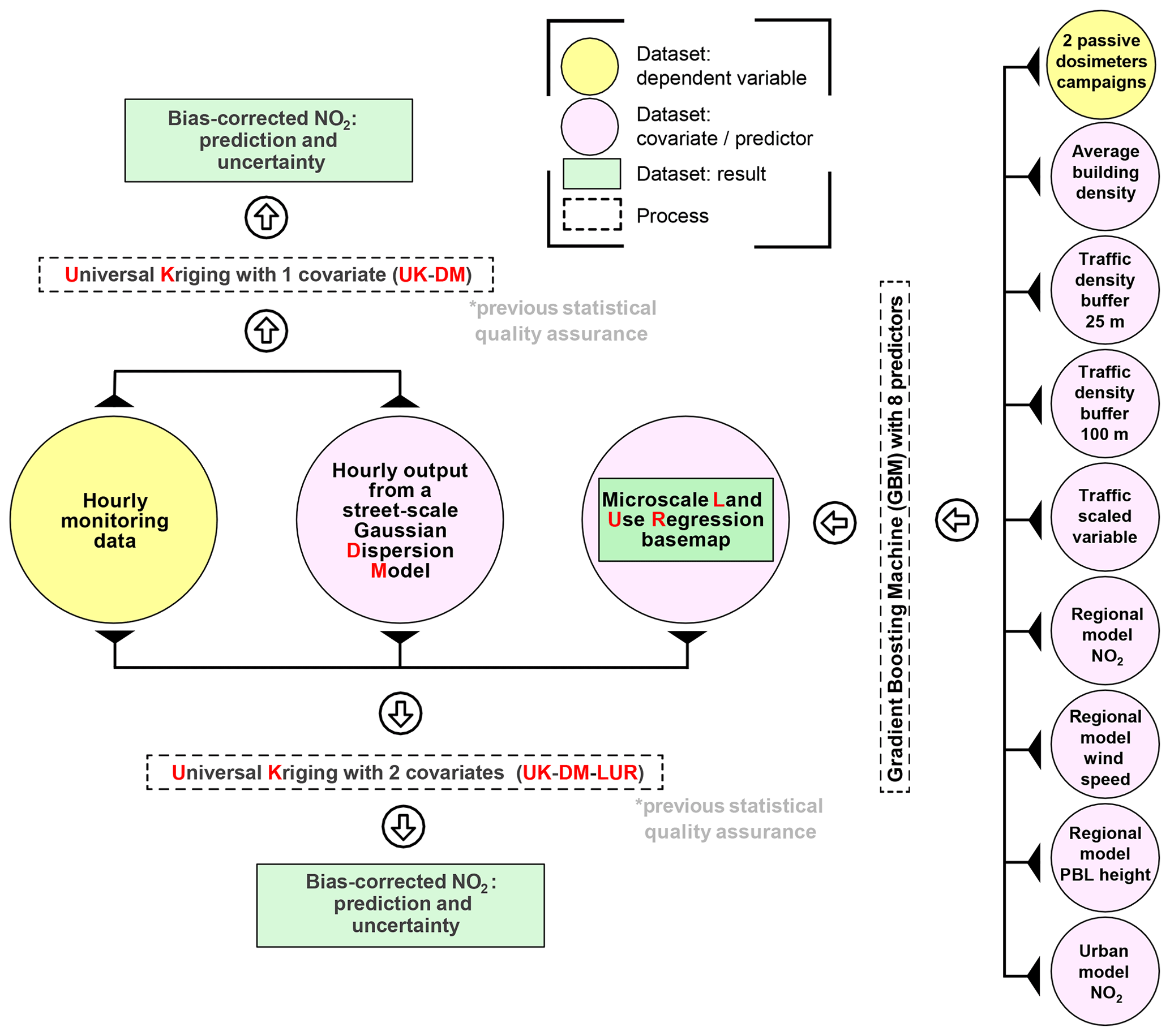
Figure 1 Workflow of the two studied data fusion methodologies. Hourly data from monitoring stations are combined with hourly dispersion model results (UK-DM) and the time-invariant microscale LUR basemap (UK-DM-LUR). PBL stands for planetary boundary layer.

2.1 Study domain and observational NO₂ data

Barcelona (Fig. 2) is the second most populated city in Spain and the 10th in Europe, with approximately 1 660 000 inhabitants and 102 km² (∼16 300 people per km²). It is located on the northeastern coast of Spain, between the Mediterranean Sea and the Collserola mountains. The city has a Mediterranean climate characterized by the dominance of a sea breeze during the warm season, shallow boundary layer development, and the recirculation of air pollutants (Jorba et al., 2004).

Hourly NO₂ observational data for 2019 are obtained from the Catalan Air Pollution Monitoring and Forecasting Network (XVPCA) measurement points in the Barcelona urban and surrounding areas. There are 13 stations available on the Barcelona agglomeration (Fig. 2), with a percentage of availability of hourly data greater than 93 %. Gràcia and Eixample are urban traffic monitoring stations, Sagnier, Observatori Fabra, and Jardins are suburban background stations, and the remaining eight correspond to urban background stations. The Observatori Fabra station is not used in our data fusion methodology since its inclusion significantly degraded the data fusion skills in the urban environment. This is expected, since the station is located on a hill relatively far from built-up areas. In fact, it is not exactly an urban station because it measures air pollution above the urban canopy, while the other stations measure pollution within the urban canopy. We are aware that, by removing this station, we may lose relevant information on the low-NO₂-level regions surrounding the city. However, the main goal of our urban model is to characterize NO₂ exceedances in critical trafficked areas. Therefore, we decided to exclude the Observatori Fabra station.

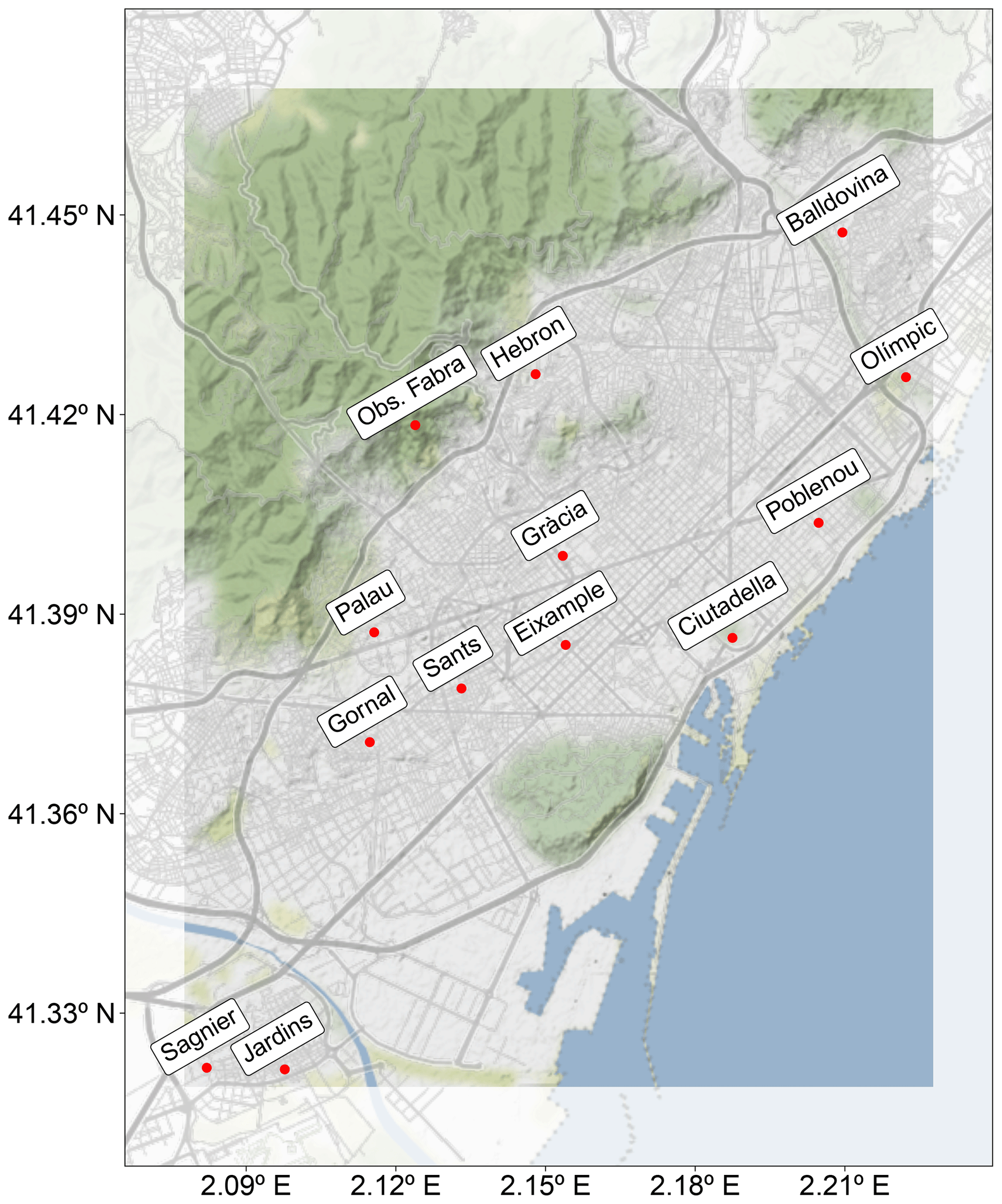
Figure 2 Domain of study and location of the referenced monitoring stations. The map has been generated using the ggplot2 (Wickham, 2016) and ggmap (Kahle and Wickham, 2013) R packages (R Core Team, 2013) and data from OpenStreetMap. © OpenStreetMap contributors 2017, distributed under the Open Data Commons Open Database License (ODbL) v1.0. Map tiles are by © Stamen Design, under a Creative Commons Attribution (CC BY 3.0) license.

Two different NO₂ passive dosimeter experimental campaigns (Fig. 3) are considered to derive the microscale LUR model, namely the xAire citizen science campaign (Perelló et al., 2021a, b) composed of 725 samplers deployed between 16 February and 15 March 2018 and the 2-week measurement campaign of the Institute of Environmental Assessment and Water Research – Spanish National Research Council (IDAEA-CSIC) that deployed 175 NO₂ samplers across Barcelona during February and March 2017 (Benavides et al., 2019). Both campaigns used Palmes-type NO₂ diffusion tubes (Palmes et al., 1976) to sample the NO₂ levels, which implies an estimated uncertainty of ±25 %, as reported in Kuklinska et al. (2015).

2.2 Street-scale air quality model: CALIOPE-Urban

Hourly high-resolution concentrations of surface NO₂ at the street scale over the city of Barcelona are estimated using the CALIOPE-Urban multiscale air quality model (Benavides et al., 2019). CALIOPE-Urban accounts for the dispersion of traffic emissions at high spatial resolution using the R-LINE Gaussian dispersion model (Snyder et al., 2013; Venkatram et al., 2013). As described in more detail in Benavides et al. (2019), R-LINE is adapted to street canyons by taking into account road link traffic emissions (Guevara et al., 2020), meteorological variables (e.g., wind speed and direction; Monin–Obukhov length and planetary boundary layer height), and building morphology (e.g., building density and height and street orientation). The chemical balance between NO_x and NO₂ is computed based on the generic reaction set (Valencia et al., 2018), assuming clear-sky conditions and uncoupling chemistry from transport phenomena. In other words, the aging of pollutants is solely a function of wind speed and the distance between the source and receptors.

At the regional scale, CALIOPE-Urban relies on the regional air quality modeling system CALIOPE (Baldasano Recio et al., 2011) for predicting the urban background NO₂ concentration. The regional CALIOPE accounts for the long-range transport of pollutants using three nested domains at increasing resolutions, namely 12 km × 12 km for the European region, 4 km × 4 km for the Iberian Peninsula, and 1 km × 1 km for the region of Catalonia (Baldasano Recio et al., 2011; Pay et al., 2014). The urban background NO₂ concentrations obtained with regional CALIOPE are combined with the R-LINE dispersion results using a dedicated parameterization of the vertical mixing (Benavides et al., 2019).

In this work, CALIOPE-Urban employs a non-uniform mesh that is refined at the edge of traffic roads and coarser in low-gradient regions of NO₂. This type of mesh accelerates the calculations and reduces memory demand. The refined grid zones have a resolution of 25 m × 25 m, progressively degrading to 500 m × 500 m in the regions of low NO₂ gradients. To facilitate their visualization, these NO₂ concentrations are finally interpolated over a uniform mesh, with a resolution of 20 m × 20 m. CALIOPE-Urban has been evaluated and successfully used in the framework of several impact studies, including the works of Benavides et al. (2021) and Rodriguez-Rey et al. (2022).

2.3 Microscale LUR model using gradient boosting machine (GBM)

A nonlinear microscale LUR model based on passive dosimeter campaigns is used to produce an observation-based climatological view of the NO₂ concentrations at a high spatial resolution over Barcelona. While the monitoring stations and the urban dispersion model provide information on the pollutants' short-term temporal behavior, the microscale LUR basemap (long-term mean) remains constant in time. Its main goal is to provide reliable long-term spatial variability patterns of NO₂ at a high resolution, using observational data and other urban information.

The target variable of the microscale LUR model is the time-averaged concentrations of the two different NO₂ experimental campaigns described in Sect. 2.1 and represented in Fig. 3. We have discarded the xAire samplers related to playgrounds and classrooms, so we are using the remaining 669. In order to combine the xAire and IDAEA-CSIC campaigns, we have annualized both, following the procedure described in Perelló et al. (2021b). For each station, an adjustment factor is computed as the ratio between the observed 2017 annual mean and the average over the period of the experimental campaign. Then, the average of this factor over all stations is used to scale all passive samplers to the 2017 annual mean. This scaling assumes that the ratio does not depend on the location and can be applied to all samplers. Despite adding some noise to the experimental results, it corrects the bias induced by environmental conditions (e.g., wind speed, atmospheric stability, precipitation, radiation, and temperature) and also allows the combining of both campaigns, producing a dataset of 844 samplers on which the microscale LUR model relies. Note that the microscale LUR model is trained using experimental campaigns deployed in February and March. As a result, even though the annualization process corrects the NO₂ levels and the predictors are expressed as annual averages, the captured spatial gradients may still have a significant seasonal bias.

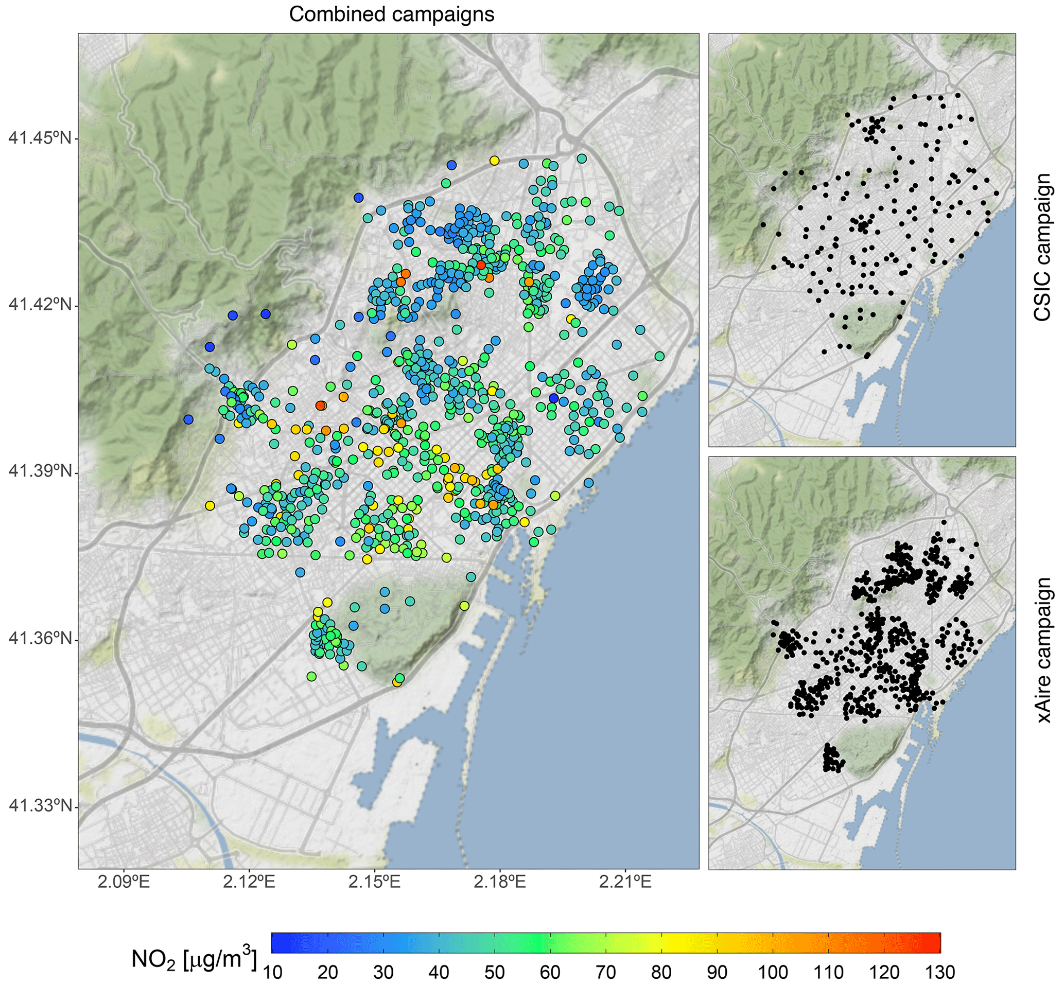
Figure 3 Sampler locations of the two different NO₂ experimental campaigns used to train the microscale LUR model. The left panel shows the NO₂ values and the locations of the combined campaigns. The top-right and bottom-right panels show the CSIC and xAire campaign locations, respectively. The color scale refers to the 2017 annualized NO₂ values (in µg m⁻³). The map has been generated using ggplot2 (Wickham, 2016) and ggmap (Kahle and Wickham, 2013) R packages (R Core Team, 2013) and data from OpenStreetMap. © OpenStreetMap contributors 2017, distributed under the Open Data Commons Open Database License (ODbL) v1.0. Map tiles are by © Stamen Design, under a Creative Commons Attribution (CC BY 3.0) license.

The potential predictors of the microscale LUR model are shown in Table 1. The geometric variables are calculated from the Institut Cartogràfic i Geològic de Catalunya (ICGC, 2019) and Plan Nacional de Ortografía Aérea (PNOA, 2020). Traffic-related predictors consist of traffic density (t) for different circular buffer sizes. With a being the radius of the buffer, t_a is computed following Eq. (1; expressed in vehicles per m s⁻¹):

$$\begin{array}{}\text{(1)}& t_a=\sum _{i=\mathrm{1}}^n{\text{AAT}}_i\cdot l_{a,i},\end{array}$$

where i represents the street segment, n is the number of street segments over the circular area of πa², l_i is the length of the street segment i within the buffer of radius a, and AAT_i is the annual average traffic of the street segment i (expressed in vehicles per second). The t_a predictors associated with the smaller buffers (5, 10, and 15 m) have highly skewed distributions, given that most values across the map are null. To avoid training the microscale LUR with skewed predictors, we introduce the traffic-scaled variable s here, which combines all buffers as follows:

$$\begin{array}{}\text{(2)}& s={\displaystyle \frac{\mathrm{1}}{N}}\sum _a{\displaystyle \frac{t_a}{\mathit{\pi }{a}^{\mathrm{2}}}},\end{array}$$

where N is the number of buffers (12 in our case). Traffic data are extracted from the road link traffic network of the HERMESv3 bottom-up emission model (Guevara et al., 2020). We also considered NO₂, the planetary boundary layer height, and the wind speed annual averages from the regional air quality modeling system CALIOPE as potential predictors, together with the NO₂ annual mean from the air quality model CALIOPE-Urban.

Table 1 The microscale LUR model contemplates the use of these 21 potential predictors.

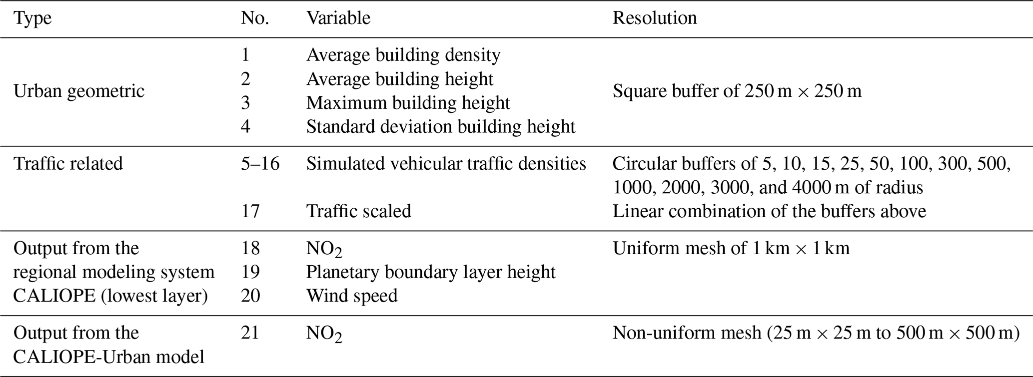
A recursive feature elimination method has been applied to remove highly correlated or uninformative features. We have used the simple backward-selection algorithm implemented in the R package caret (Kuhn, 2008), which starts with the full-featured model and gradually removes the least important feature, while monitoring the RMSE in cross-validation (CV). The goal is to obtain the simplest model with the lowest RMSE to gain generalization and interpretability. The final microscale LUR model includes the following eight predictors: average building density, traffic buffers of 25 and 100 m, traffic-scaled variable s, all the annually averaged data from the regional CALIOPE modeling system (NO₂, the planetary boundary layer height, and the wind speed), and the NO₂ annual mean from CALIOPE-Urban.

To account for nonlinear relations among the predictors and the target variable, we used the gradient boosting machine (GBM) algorithm implemented in the R package gbm (Greenwell et al., 2022). GBM is a popular machine learning algorithm (Natekin and Knoll, 2013) that has shown excellent results in terms of accuracy and generalization when compared to other learning algorithms (Caruana and Niculescu-Mizil, 2006). The GBM hyperparameters (shrinkage rate, interaction depth, minimum observation per node, and bag fraction) are optimized based on the minimum mean cross-validated error and a grid search algorithm. Additionally, following the work of Chen et al. (2019), we exploit the potential spatial correlation of the GBM residuals by interpolating and adding them to the predicted values. The interpolation is done with ordinary kriging (Wackernagel, 2003).

One could think that skipping over the LUR computation by directly using all of its time-invariant information (passive dosimeter campaigns, urban geometry, traffic-related data, and annually averaged model results) as covariates in the universal kriging methodology would simplify the workflow. However, there are two main drawbacks to doing so. On the one hand, in contrast to GBM, universal kriging assumes linear relations between covariates and the observed NO₂, which is not necessarily true for this case. On the other hand, when considering a large number of covariates with only 12 monitoring stations, strong spurious correlations lacking physical meaning are prone to happen, which drive the final solution wrongly (Hengl et al., 2007). Thus, gathering all static information into a single LUR covariate offers more robust results, while permitting the addition of predictors using nonlinear regression models.

2.4 Universal kriging as a data fusion methodology for spatial bias correction

The microscale LUR model and the hourly CALIOPE-Urban outputs are combined with observational NO₂ data from the monitoring stations using the geostatistical technique of universal kriging, which is commonly used for spatial interpolation. This methodology predicts a random variable Z at a target point x, based on a combination between a (multi-)linear regression analysis with external variables f, referred to as covariates, and a pure spatial interpolation considering the autocorrelation structure of the regression residuals. In our case, the variable Z corresponds to the monitoring data, while the covariates are CALIOPE-Urban and our microscale LUR model. A simple (multi-)linear regression model is convenient here, given the low number (12) of available monitoring stations within the computational domain. Universal kriging assumes the following relation (Cressie, 1993):

$$\begin{array}{}\text{(3)}& Z\left(\mathbf{x}\right)=\sum _{l=\mathrm{0}}^L{a}_{\mathrm{l}}{f}_{\mathrm{l}}\left(\mathbf{x}\right)+R\left(\mathbf{x}\right),\end{array}$$

where L equals 1 in the UK-DM approach and 2 in the UK-DM-LUR, a_l are the non-zero coefficients from the (multi-)linear regression between the observations and the covariates f_l (with f₀(x)=1 by convention), and R(x) is the residual random field. The deterministic part of the variable Z is explained by a linear combination of the covariates, while the residual random field is considered to have zero mean and to be spatially autocorrelated. The main advantage of this method is that, depending on the strength of the correlation between covariates and observations, universal kriging gives more weight either to the (multi-)linear regression or to the spatial interpolation of the residuals (Hengl, 2009), thus providing a robust data fusion method that adapts to the quality of the model output.

As a Gaussian process, universal kriging estimates the variance of its predictions (σ²) coming from both the (multi-)linear regression (${\mathit{\sigma }}_{\mathrm{MLR}}^{\mathrm{2}}$) and the spatial interpolation (${\mathit{\sigma }}_{\mathrm{SI}}^{\mathrm{2}}$) steps, as follows:

$$\begin{array}{}\text{(4)}& {\mathit{\sigma }}^{\mathrm{2}}\left(\mathbf{x}\right)=\underset{{\mathit{\sigma }}_{\mathrm{SI}}^{\mathrm{2}}}{\underbrace{\sum _{\mathit{\alpha }=\mathrm{1}}^m{w}_{\mathit{\alpha }}\cdot {\mathit{\gamma }}_R({\mathbf{x}}_{\mathit{\alpha }}-\mathbf{x})}}+\underset{{\mathit{\sigma }}_{\mathrm{MLR}}^{\mathrm{2}}}{\underbrace{\sum _{l=\mathrm{0}}^L{\mathit{\lambda }}_{\mathrm{l}}{f}_{\mathrm{l}}\left(\mathbf{x}\right)}},\end{array}$$

where m is the number of monitoring stations, w_α are the spatial interpolation weights associated with each measurement point, λ_l are the L+1 Lagrangian multipliers used to minimize the variance error, and γ_R(x_α−x) stands for the variogram which characterizes the spatial structure of the residuals (Chiles and Delfiner, 1999). Thus, the variance of a prediction reflects how far the unmeasured location is from the observation points and from the feature space in which the regression model has been calibrated, i.e., the extrapolation effect (Hengl, 2009). Our universal kriging implementation relies on the R package gstat (Pebesma, 2004; Gräler et al., 2016).

To normalize the distribution of the NO₂ data and to ensure positive predicted values, we have applied the universal kriging technique described above after transforming NO₂ data into the log space. However, the results need to be back-transformed to the original scale. Following the work of Cressie (1993), the back-transformation is performed as follows:

$$\begin{array}{}\text{(5)}& {\displaystyle }\widehat{Z}\left(\mathbf{x}\right)=\exp \left(Z_{\mathrm{l}}\right(\mathbf{x})+{\mathit{\sigma }}_{\mathrm{l}}^{\mathrm{2}}(\mathbf{x})/\mathrm{2}),\text{(6)}& {\displaystyle }{\widehat{\mathit{\sigma }}}^{\mathrm{2}}\left(\mathbf{x}\right)=\left(\exp \right({\mathit{\sigma }}_{\mathrm{l}}^{\mathrm{2}}\left(\mathbf{x}\right))-\mathrm{1})\cdot \exp (\mathrm{2}\cdot Z_{\mathrm{l}}(\mathbf{x})+{\mathit{\sigma }}_{\mathrm{l}}^{\mathrm{2}}(\mathbf{x}\left)\right),\end{array}$$

where $\widehat{Z}\left(\mathbf{x}\right)$ and ${\widehat{\mathit{\sigma }}}^{\mathrm{2}}\left(\mathbf{x}\right)$, respectively, represent the back-transformed prediction and variance at the target point, while Z_l(x) and ${\mathit{\sigma }}_{\mathrm{l}}^{\mathrm{2}}\left(\mathbf{x}\right)$ are the prediction and variance in the log space, respectively.

Assuming a normal distribution of the error, the probability of exceedance (𝒫) of a certain limit value (ℒ) can be computed as follows (Horálek et al., 2008):

$$\begin{array}{}\text{(7)}& \mathcal{P}\left(\mathbf{x}\right)=\mathrm{1}-F\left({\displaystyle \frac{\mathcal{L}-\widehat{Z}\left(\mathbf{x}\right)}{\widehat{\mathit{\sigma }}\left(\mathbf{x}\right)}}\right),\end{array}$$

where F is the normal cumulative distribution function.

2.4.1 Statistical metrics to evaluate data fusion skills

Statistical performance is assessed by leave-one-out cross-validation (LOOCV), which consists of performing the data fusion by considering all of the monitoring stations, except for one that is kept to cross-validate the results. For each LOOCV, we present the coefficient of efficiency (COE), the root mean square error (RMSE), the mean bias (MB), and the correlation coefficient (r), defined as follows:

$$\begin{array}{}\text{(8)}& {\displaystyle }\text{COE}=\mathrm{1}-{\displaystyle \frac{{\sum }_{i=\mathrm{1}}^k\mathrm{|}{M}_i-O_i\mathrm{|}}{{\sum }_{i=\mathrm{1}}^k\mathrm{|}{O}_i-O\mathrm{|}}}\text{(9)}& {\displaystyle }\text{MB}={\displaystyle \frac{\mathrm{1}}{k}}\sum _{i=\mathrm{1}}^k{M}_i-O_i\text{(10)}& {\displaystyle }r={\displaystyle \frac{\mathrm{1}}{k-\mathrm{1}}}\sum _{i=\mathrm{1}}^k\left({\displaystyle \frac{M_i-M}{{\mathit{\sigma }}_M}}\right)\left({\displaystyle \frac{O_i-O}{{\mathit{\sigma }}_O}}\right)\text{(11)}& {\displaystyle }\text{RMSE}=\sqrt{{\displaystyle \frac{\mathrm{1}}{k}}\sum _{i=\mathrm{1}}^k(M_i-O_i{)}^{\mathrm{2}}},\end{array}$$

where k is the total number of observations, O_i and M_i are the observed and modeled i values, respectively, O and M are their respective means, and σ_O and σ_M refer to their standard deviation.

2.4.2 Spatial autocorrelation structure of NO₂ levels

In the universal kriging context, the variogram describes the spatial autocorrelation structure of the residual random field. In our case, the limited number of monitoring stations makes it challenging to extract a meaningful spatial structure. For this reason, we estimate the residual variogram based on the dosimeter campaigns. This decision, however, entails a substantial limitation due to the assumption of a static variogram. We rely only on the IDAEA-CSIC campaign (discarding the xAire campaign for the variogram derivation) to avoid extra premises for the combination of campaigns. Additionally, we considered an isotropic variogram. All of these postulates impact the variance error estimated by universal kriging (Brus and Heuvelink, 2007). To assess the impact of such assumptions, an analysis of the estimated variance in LOOCV is carried out in Sect. 3.2.

The variogram is fitted using the Matérn model with Stein's parameterization implemented in the R package automap (Hiemstra et al., 2009), setting the smoothing parameter κ=0.2. The resulting variogram model is characterized by a $\mathrm{5}\times {\mathrm{10}}^{-\mathrm{2}}$ partial sill, $\mathrm{3}\times {\mathrm{10}}^{-\mathrm{5}}$ nugget, and a range of 620 m. Following the work of Denby et al. (2007), we have optimized the range value to minimize the RMSE of universal kriging. The range estimates the distance at which the data are no longer correlated. To optimize it, we performed an hourly LOOCV by varying the range from 1 to 10 km for every 1 km, while keeping all other model parameters constant. We obtained the best results for the range of 5 km, which improved the r coefficient by 4 %, the COE by 14 %, and the RMSE by −9 % on average over all monitoring stations, compared to the UK-DM-LUR methodology that used the original range of 620 m.

2.4.3 Statistical quality assurance of the (multi-)linear regression

The correlation coefficient (r) and the regression coefficient (slope) of the regression model between covariates (CALIOPE-Urban and the microscale LUR model) and observations are checked before the covariates are included in the universal kriging workflow (as indicated in Fig. 1). If a covariate shows a low correlation (p value >0.05) with the observations at a specific hour, then it is not considered in the regression model, as in the works of Zhang et al. (2021) and Oh et al. (2021). Additionally, if none of the covariates shows a significant correlation, then we use both covariates to build the regression model. However, to avoid nonphysical hourly maps, the covariates are used only if their regression coefficient is positive, as suggested by Denby et al. (2007). In case all of the regression coefficients are negative, or there are fewer than four observations available in a specific hour, universal kriging is not performed, and the results of the data fusion method are directly the raw dispersion–model output. Following the above criteria, the percentage of cases with fewer than four monitoring observations is relatively small, 0.034 % (3 h), and is the same for each kriging application. For the UK-DM methodology, 14.11 % of the hours have not been corrected due to negative regression coefficients. On the other hand, for the case of UK-DM-LUR, only 1.47 % of the hours have been discarded due to a negative regression coefficient in both covariates. As Benavides et al. (2019) identified, the poor skills of the urban model are attributed to low wind speeds and atmospheric stability situations, which cause the performance of the mesoscale model to decrease. Concerning the static microscale LUR basemap, the poor correlation on an hourly basis is associated with hours that significantly deviate from the average behavior.

3 Results and discussion

The results are organized into two sections. First, in Sect. 3.1, we estimate the microscale LUR model performance and present the obtained NO₂ basemap. Second, in Sect. 3.2, the data fusion methodologies are discussed in terms of statistical performance, uncertainty quantification, and exceedance probability maps. All the maps presented in this section have been generated using the ggplot2 (Wickham, 2016) and ggmap (Kahle and Wickham, 2013) R packages (R Core Team, 2013) and data from Open Data BCN (Ajuntament de Barcelona, 2019) and OpenStreetMap (© OpenStreetMap contributors 2017, distributed under the Open Data Commons Open Database License (ODbL) v1.0. Map tiles are by © Stamen Design, under a Creative Commons Attribution (CC BY 3.0) license).

3.1 Microscale LUR model

3.1.1 Performance assessment

The GBM-based microscale LUR model is evaluated using two nested K-fold CVs, with the inner one for tuning the model (training–validation set) and the outer one for testing the model on different parts of the dataset (test set). Such a procedure aims at giving a reliable estimate of the expected performance. We use an outer 10-fold CV and an inner 4-fold CV, as illustrated in Fig. 4. The tuning of the model is performed through a grid search over the following hyperparameters: shrinkage rate (with values ranging from 0.001 to 0.05 every 0.001), the interaction depth (from 1 to 4 every 1), the minimum observation in a node (from 5 to 15 every 1), and the bag fraction (0.5 and 0.65).

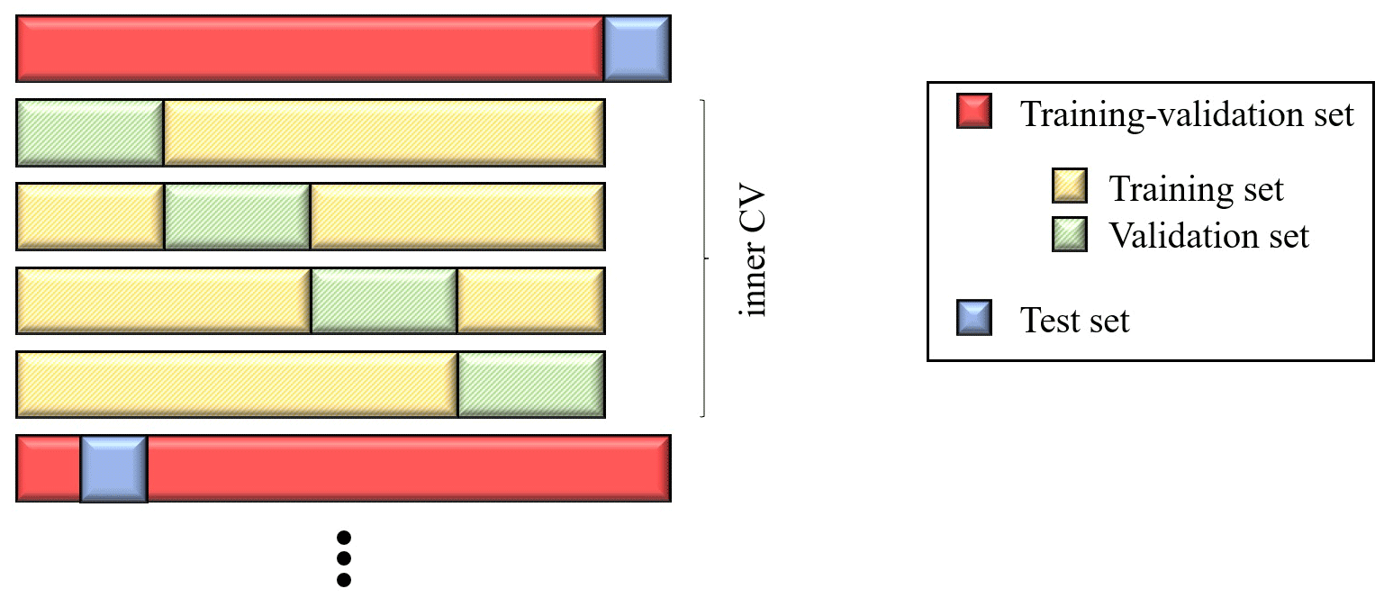
Figure 4 Scheme of the outer 10-fold CV and the inner 4-fold CV applied for the GBM training.

The results are given in Table 2, together with the performance reference of the annual mean NO₂ concentration obtained directly from CALIOPE-Urban. As explained in Sect. 2.3, we exploit the spatial autocorrelation of the LUR residuals to improve its estimation. To do so, the microscale LUR residuals at the training locations are interpolated at the test locations by applying an ordinary kriging. Then, they are added to the predictions to obtain the corrected results (see values for “test set adding the residuals” in Table 2).

Table 2 Statistical results of the microscale LUR model in nested CV. The 2017 annual mean concentration of NO₂ of the raw dispersion model (CALIOPE-Urban) is also shown. The parameter n stands for the number of data points used to compute the statistics.

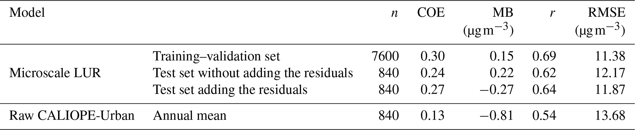
Table 2 shows that the microscale LUR model significantly improves the CALIOPE-Urban results. Also, the addition of the residuals slightly increases the statistical performance. The training–validation set results are not perfectly fitted and are only slightly better than the test set results, indicating that the microscale LUR is not overfitted and has good capabilities for the prediction of unseen data.

In Fig. 5, we show the scatterplots of the CALIOPE-Urban annual mean and the test set results with and without adding the residuals, along with the observational uncertainty ranges indicated by the dashed red lines (±25 %, according to Kuklinska et al., 2015). Although a large portion of the predicted values for the microscale LUR model with the residual correction lies within the uncertainty range, difficulty can be observed in predicting values of NO₂ higher than 80 µg m⁻³. We attribute this behavior to not only the limited number of points in this range, which can weaken the model training, particularly in the nested CV context, but also to the already poor predictive skills of CALIOPE-Urban in this concentration range (as seen in Fig. 5a).

Figure 5 (a) Raw annual mean of CALIOPE-Urban NO₂ concentrations, (b) microscale LUR model results, without the interpolated residuals, and (c) microscale LUR model results, with the interpolated residuals, versus the annualized passive dosimeter campaigns. These figures use the test sets in which the performance of the microscale LUR model has been assessed. The dashed red lines report passive dosimeter uncertainty (±25 %), and the identity line is represented in blue. The statistical results are shown in Table 2.

Comparing these results with previous works, the resulting correlation coefficient (r) is lower than a LUR model fitted with the xAire campaign data (r=0.74 in LOOCV), as reported in Perelló et al. (2021a). However, Perelló et al. (2021a) used only 370 outdoor sampling sites out of the 669 available. They excluded samplers close to traffic and street intersections, achieving a skilled urban LUR model. Even if the r coefficient is slightly lowered, we have considered all outdoor sampling sites (along with the IDAEA-CSIC campaign) to capture, as much as possible, the NO₂ spatial trends. On the other hand, the work of Munir et al. (2020) reported a microscale LUR model based on 40 time-dependent LCSs with slightly lower performance in the CV than the present one (r=0.56). Moreover, Munir et al. (2020) also reported a r value of 0.53 when the nonlinear LUR model is based on the combination of 188 period-averaged and 40 time-dependent LCSs. A key aspect of the present data fusion methodology is that the microscale LUR model results explain better the annualized passive dosimeter campaigns compared to the reference CALIOPE-Urban annual mean. Therefore, they are subsequently considered to be a covariate in the universal kriging methodology, as further explained in Sect. 3.1.2. An assessment regarding the necessary number of samplers to derive a robust microscale LUR is presented in Appendix A.

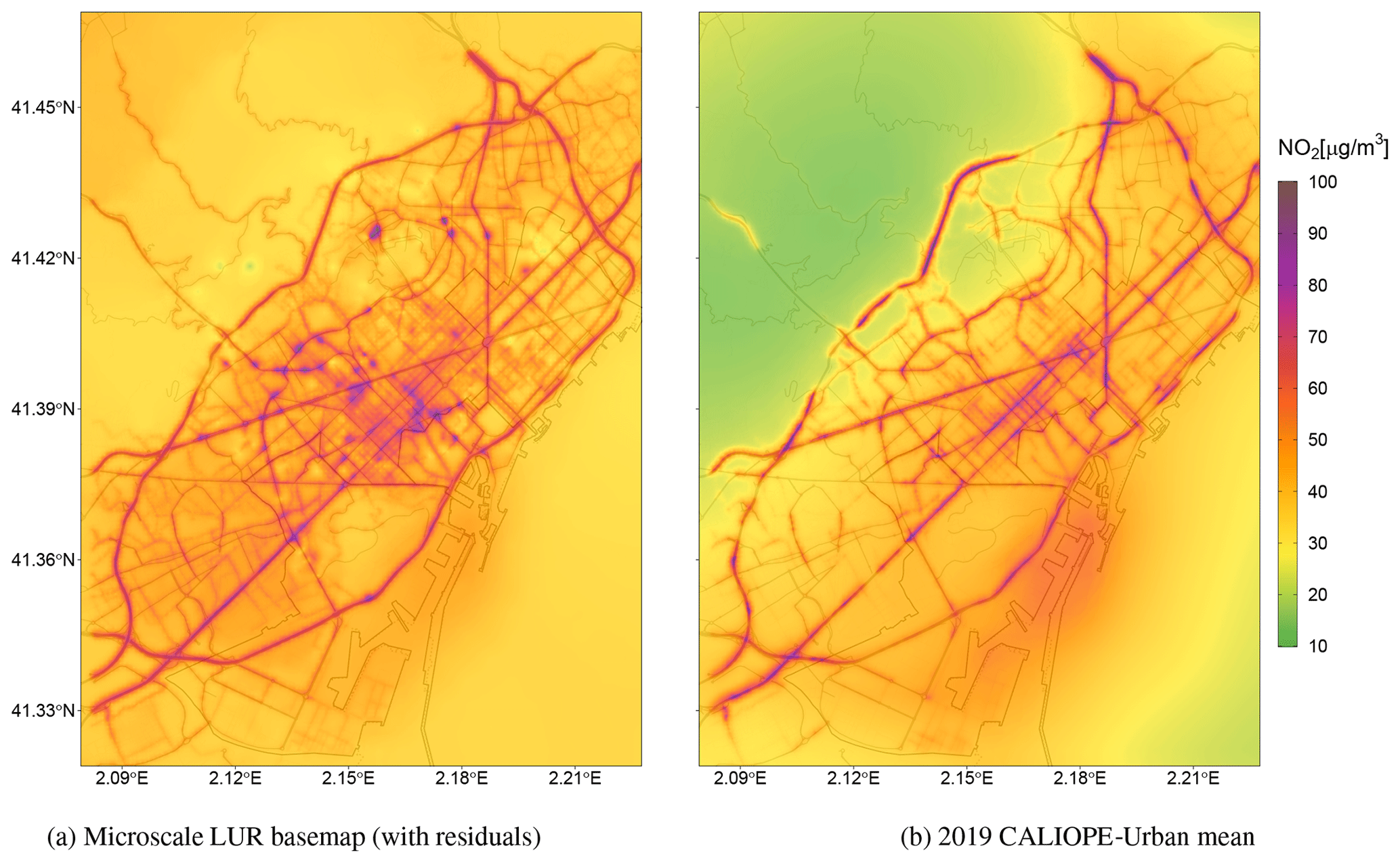
Figure 6 (a) Resulting microscale LUR basemap using all available sampling sites and adding the interpolated residuals. (b) The 2019 annual mean concentration of NO₂ of the raw dispersion model CALIOPE-Urban.

3.1.2 Microscale LUR basemap

We proceed to train the microscale LUR model with the residual correction using all available sampling sites. Figure 6 compares the long-term NO₂ patterns from the microscale LUR basemap (Fig. 6a) with the NO₂ 2019 annual mean of CALIOPE-Urban (Fig. 6b). Notice that the goal of the basemap is to correct the long-term spatial variability in NO₂. Thus, Fig. 6 highlights the differences in spatial patterns rather than differences in absolute NO₂ values. The resulting basemap shows a qualitatively consistent NO₂ distribution; the major trafficked roads of the city and the port area are the most polluted locations, while the Collserola mountains and the sea bordering the city have moderate NO₂ levels. Although both figures show similar NO₂ patterns, local differences from experimental information can be observed in Fig. 6a. For instance, there is a noticeable increase in NO₂ levels for the microscale LUR basemap in the mountainous northwestern area of the study domain. This artifact is probably caused by the spatial distribution of the passive dosimeter campaigns (Fig. 3), which poorly cover this region. The NO₂ overprediction of this area is not reflected in the statistical evaluation of the data fusion since we deliberately omitted the monitoring station located in this area. We excluded this station to improve the data fusion model's ability to capture NO₂ exceedances in built-up areas, which is the main goal of the urban model. As further shown in the statistical results, considering extensive passive dosimeters information through the microscale LUR model avoids relying only on the urban model to describe the NO₂ gradients and significantly improves the data fusion methodology.

The influence of each predictor in the final microscale LUR model has been computed based on the methodology proposed by Friedman (2001) and implemented in the R package gbm (Greenwell et al., 2022), in which the relative importance of each variable is associated with the reduction in the GBM cost function. Given the chosen set of predictors, the most influential variable is the NO₂ CALIOPE-Urban annual mean with a relative importance of 25.1 %, followed by 17.7 % for the traffic scaled variable and 15.7 % for the average building density. The other predictors exhibited a relative influence under the 15 %, with the NO₂ CALIOPE regional annual mean as the lowest one with 4.3 %.

3.2 Data fusion methodologies

3.2.1 Statistical evaluation

In order to quantify the added value of including the microscale LUR basemap in the data fusion methodology, two different post-processes (see Fig. 1) have been carried out. First, the output of the urban dispersion model CALIOPE-Urban is merged with the monitoring data using universal kriging, named UK-DM. Second, the microscale LUR basemap is added as a covariate in the universal kriging workflow, named UK-DM-LUR.

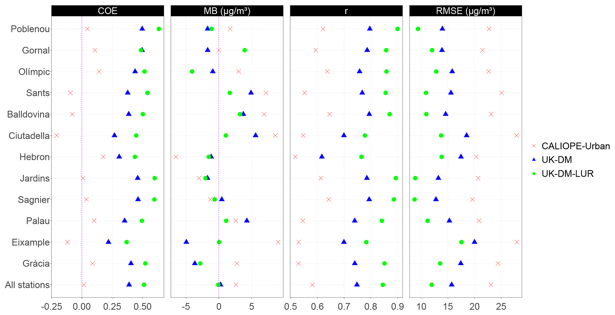
Figure 7 Statistical results for each station after applying UK-DM and UK-DM-LUR to 2019 hourly data in LOOCV. In addition, we show the statistical results for the CALIOPE-Urban estimates at each station. All stations refer to the average over all stations.

Hourly statistical results for the raw CALIOPE-Urban, UK-DM, and UK-DM-LUR models are shown in Fig. 7 for each monitoring station using all available data of 2019. UK-DM and UK-DM-LUR results have been computed in LOOCV, as explained in Sect. 2.4. Gràcia and Eixample are the urban traffic monitoring stations, and the last row in Fig. 7 corresponds to the average results over all stations. This figure shows that the hourly scale post-processing consistently improves all studied statistical metrics at all monitoring stations, regardless of their type. Moreover, adding the microscale LUR basemap as a covariate (UK-DM-LUR) further improves the spatial correction at all stations and for all statistical metrics, except for the MB, which does not have a clear trend. A negative COE value reflects a poor predictive capacity, so we highlight that both data fusion methods achieve a positive COE at all considered stations. Almost all stations show a positive MB for CALIOPE-Urban, indicating a general overestimation of the model, while UK-DM and UK-DM-LUR present almost null MB averaged over all stations. The overestimation of CALIOPE-Urban in the monitoring stations may seem contradictory, with the negative bias presented in Table 2 for the passive dosimeter campaigns. However, this could indicate that the highest NO₂ values in Barcelona are not routinely monitored, as already pointed out in the work of Duyzer et al. (2015b). Regarding the RMSE, the averaged reduction between CALIOPE-Urban and UK-DM is about 32 % and 24 % between UK-DM and UK-DM-LUR. For the r coefficient, an averaged improvement of 29 % between CALIOPE-Urban and UK-DM is observed, while the improvement between UK-DM and UK-DM-LUR is 13 %.

3.2.2 Uncertainty quantification

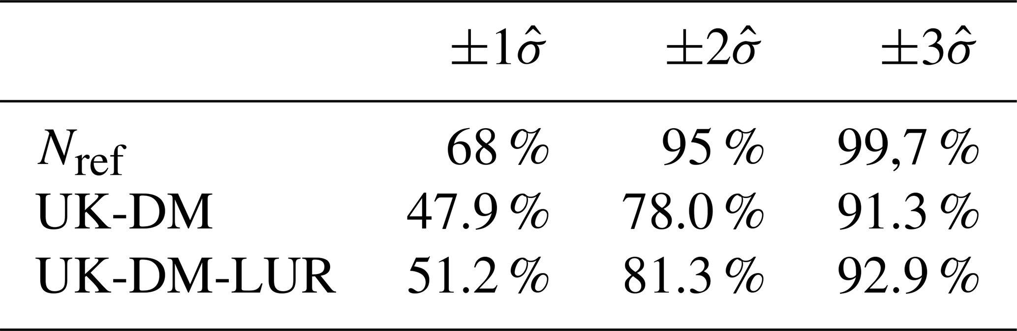
The uncertainty in the universal kriging predictions is estimated from the (multi-)linear regression and the spatial interpolation variances, as formulated in Eq. (4). The spatial interpolation is based on the variogram, which has been modeled from a period-averaged passive dosimeter campaign; thus, it assumes a static behavior, as pointed out in Sect. 2.4.2. Additionally, the variogram is considered isotropic for simplicity, while we know that, in the urban scale, the NO₂ autocorrelation structure may vary significantly, depending on the direction with respect to traffic road links. These assumptions directly impact the error variance estimated by the universal kriging, ${\widehat{\mathit{\sigma }}}^{\mathrm{2}}$. Considering that the interpolation error is normally distributed (N_ref), the observation at a specific monitoring station when performing a LOOCV should be within $\pm \widehat{\mathit{\sigma }}$ of the predicted value for 68 % of the time, while being 95 % and 99.7 %, respectively, for $\pm \mathrm{2}\widehat{\mathit{\sigma }}$ and $\pm \mathrm{3}\widehat{\mathit{\sigma }}$, as indicated in Table 3. To assess the normality of these distributions, Table 3 reports an empirical validation of the percentage of observations falling within the corresponding error range, again computed in LOOCV. These percentages show that the uncertainty is underpredicted for both methods. However, the overconfident UK-DM-LUR results are slightly better than the UK-DM ones.

Table 3 Percentages of observations falling in the $\pm \widehat{\mathit{\sigma }}$, $\pm \mathrm{2}\widehat{\mathit{\sigma }}$, $\pm \mathrm{3}\widehat{\mathit{\sigma }}$ confidence intervals, using all stations in LOOCV during 2019. Confidence intervals are computed based on the hourly predicted values and their standard deviation.

To better understand the behavior of uncertainty estimates, in Fig. 8 we show the probability density functions (PDFs) of the hourly bias, normalized by the error standard deviation $\widehat{\mathit{\sigma }}$, for UK-DM and UK-DM-LUR, using all studied monitoring stations in LOOCV over all available hours in 2019. The error PDFs have normal trends with a slightly negative skew and are overconfident, in accordance with Table 3. Both methodologies, especially UK-DM, exhibit negative skewness. This is because the corrected model struggles to capture the infrequent high-pollution peaks, tending to underestimate them significantly instead. Thus, negative biases (M_h<O_h) are rare but stronger. On the other hand, the model tends to overpredict moderate observed values slightly. Therefore, positive biases (M_h>O_h) are more frequent and less severe. In agreement with the overall null bias, the rare strong underestimations are compensated by frequent moderate overestimations.

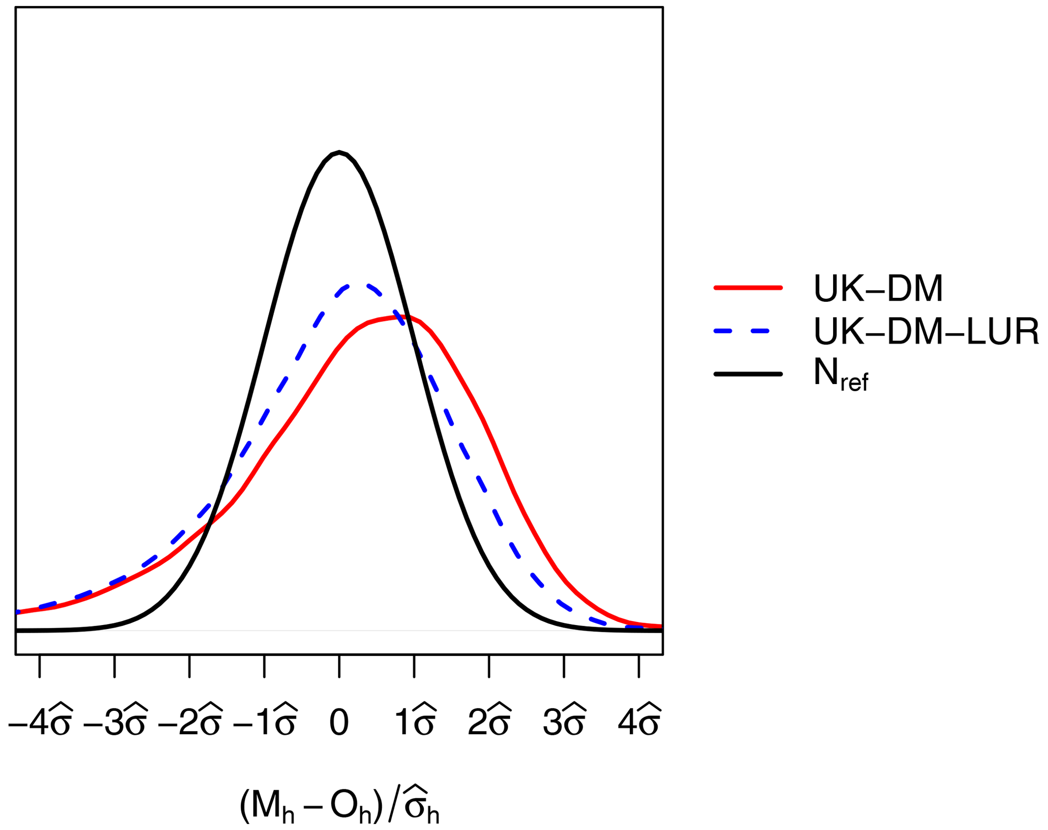
Figure 8 PDF of the hourly bias, normalized by the universal kriging standard deviation, for all monitoring stations in LOOCV during 2019. The PDFs correspond to the reference normal distribution (N_ref), UK-DM, and UK-DM-LUR hourly results.

In addition, in Fig. 9, the PDFs are computed by splitting the observed NO₂ concentration levels in three different ranges, namely less than 40 µg m⁻³, greater than 100 µg m⁻³, and between 40 and 100 µg m⁻³. These PDFs allow us to study the behavior of the error distribution for different NO₂ values. This figure shows that larger concentration levels tend to be underestimated, while the smaller ones are overestimated. In all ranges and for both methodologies, the normal trends of the error PDFs are conserved, with the intermediate ranges being the closest to the theoretical normal distribution.

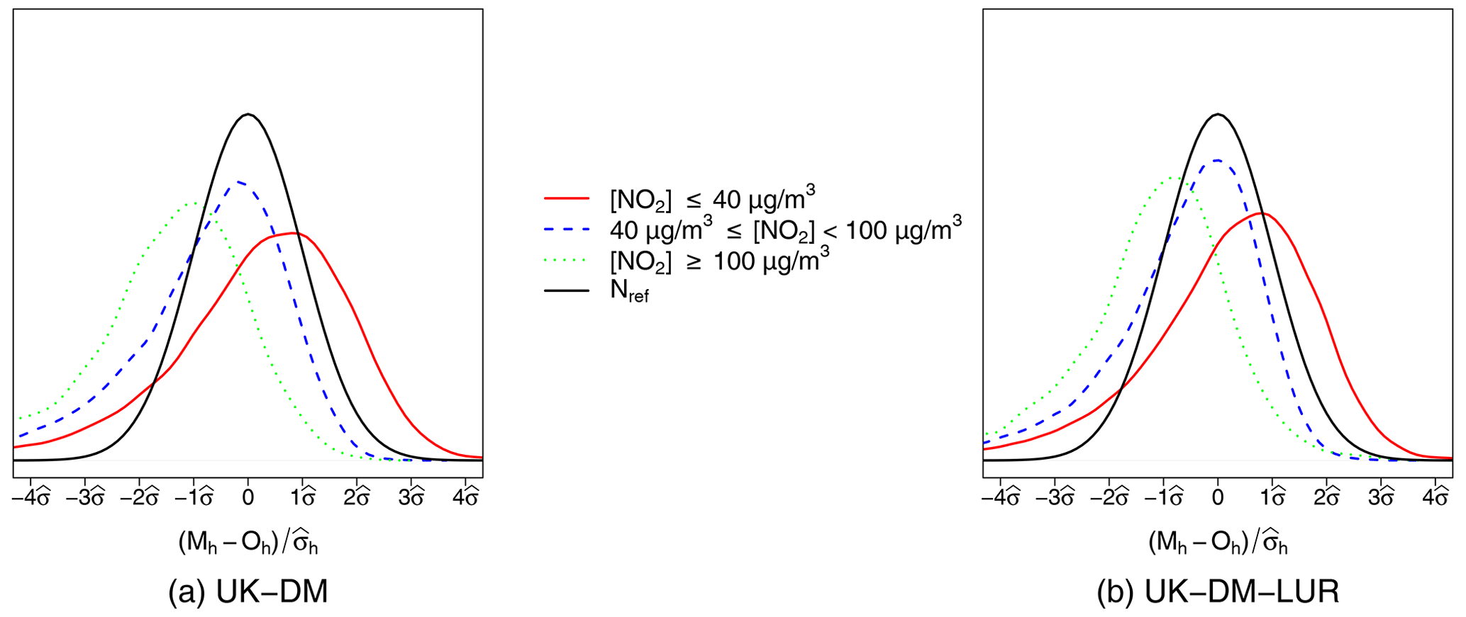
Figure 9 PDFs by observed NO₂ ranges of the hourly bias, normalized by the standard deviation error, for all monitoring stations in LOOCV during 2019 for (a) UK-DM and (b) UK-DM-LUR applications.

3.2.3 Street-scale maps

We first analyze the annual mean concentration levels of NO₂. Table 4 presents the evaluation in LOOCV of the results post-processed by the UK-DM and the UK-DM-LUR methodologies applied directly to the 2019 annual mean. The presented statistics are computed using a single NO₂-averaged value for each station. The annually based statistics are similar to the hourly results shown in Fig. 7. However, there is a substantial drop in the RMSE associated with the bias compensation when averaging the hourly data.

Table 4 Statistical results using the 12 monitoring stations after applying UK-DM and UK-DM-LUR directly to the annual averages in LOOCV.

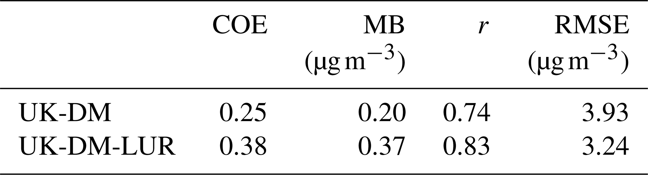
Figure 10 (a) NO₂ 2019 annual map resulting from applying UK-DM with the annual values. (b) Relative uncertainty associated with the predictions in panel (a). (c) Annual probability map of values exceeding the 40 µg m⁻³ NO₂ limit, using the values in panels (a) and (b). (d) NO₂ 2019 annual map resulting from applying UK-DM-LUR with the annual values. (e) Relative uncertainty associated with the predictions in panel (d). (f) Annual probability map of values exceeding the 40 µg m⁻³ NO₂ limit, using the values in panels (d) and (e).

Figure 10 presents the NO₂ annual mean, its associated relative uncertainty, and the probability map of values exceeding the NO₂ annual limit value of 40 µg m⁻³ (AAQD 2008/EC/50) for both UK-DM and UK-DM-LUR methodologies. The annual mean levels combining the raw model with the monitoring stations data (UK-DM; Fig. 10a) have similar trends to the raw CALIOPE-Urban (Fig. 6b). However, pollution levels are significantly reduced. Adding the passive dosimeter information through the microscale LUR basemap (UK-DM-LUR; Fig. 10d) slightly increases NO₂ concentrations, particularly in the city center and secondary roads, where the microscale LUR basemap (Fig. 6a) exhibits steeper NO₂ gradients than CALIOPE-Urban (Fig. 6b).

As expected, the areas surrounding the monitoring stations (presented in Fig. 2) show lower relative uncertainty, as can be seen in Fig. 10b and e. The higher uncertainty regions, on the other hand, correspond to areas far from the monitoring sites, and areas with extreme concentration levels, which causes an extrapolation effect in the regression model. When comparing the two uncertainty maps (Fig. 10b and e), UK-DM-LUR has regions with higher relative uncertainty than UK-DM. This behavior is due to the addition of the microscale LUR covariate, which increases the standard deviation associated with the regression model. In addition, some localized regions of high uncertainty can be observed in Fig. 10e. They are associated with the locations of the passive dosimeters and trafficked roads, where the microscale LUR covariate has caused an increase in NO₂ concentrations, thereby raising the level of extrapolation in the regression model. The high uncertainty values in the upper-left corner of Fig. 10b and e correspond to the low NO₂ levels predicted in the Collserola mountains. These high-uncertainty values can be reduced by considering the Observatori Fabra station, which is located in this area. However, as explained in Sect. 2.1, we excluded this station since its inclusion decreases the data fusion model's ability to predict high NO₂ values in critical trafficked areas.

Regardless of the data fusion method, the most polluted regions correspond to probabilities exceeding the annual limit above 0.7, as shown in Fig. 10c and f. When considering the UK-DM-LUR method, 13 % of the Barcelona municipality area has a 0.7 or higher probability of exceeding the annual limit, and this percentage rises to 30 % when considering probabilities equal to or higher than 0.5. The Eixample district, which is the most polluted, while being the most populous and densely populated (approximately 270 000 inhabitants and 36 000 inhabitants per square kilometer, according to Ajuntament de Barcelona, 2019), has 95 % of its area exceeding the annual limit, with a probability equal to or higher to 0.5 and 69 % in the case of 0.7. Thus, significant evidence indicates that the NO₂ annual legal limit was broadly exceeded in Barcelona in 2019. Stronger evidence could be obtained by reducing the uncertainty associated with the results, either by using a better-correlated urban model or by increasing the monitoring system's coverage. To test a more restrictive threshold, we have analyzed the annual exceedance probability maps using the recommended WHO 2021 annual limit of 10 µg m⁻³ (WHO, 2021), obtaining probabilities above 0.9 across the domain for both methodologies (not shown here).

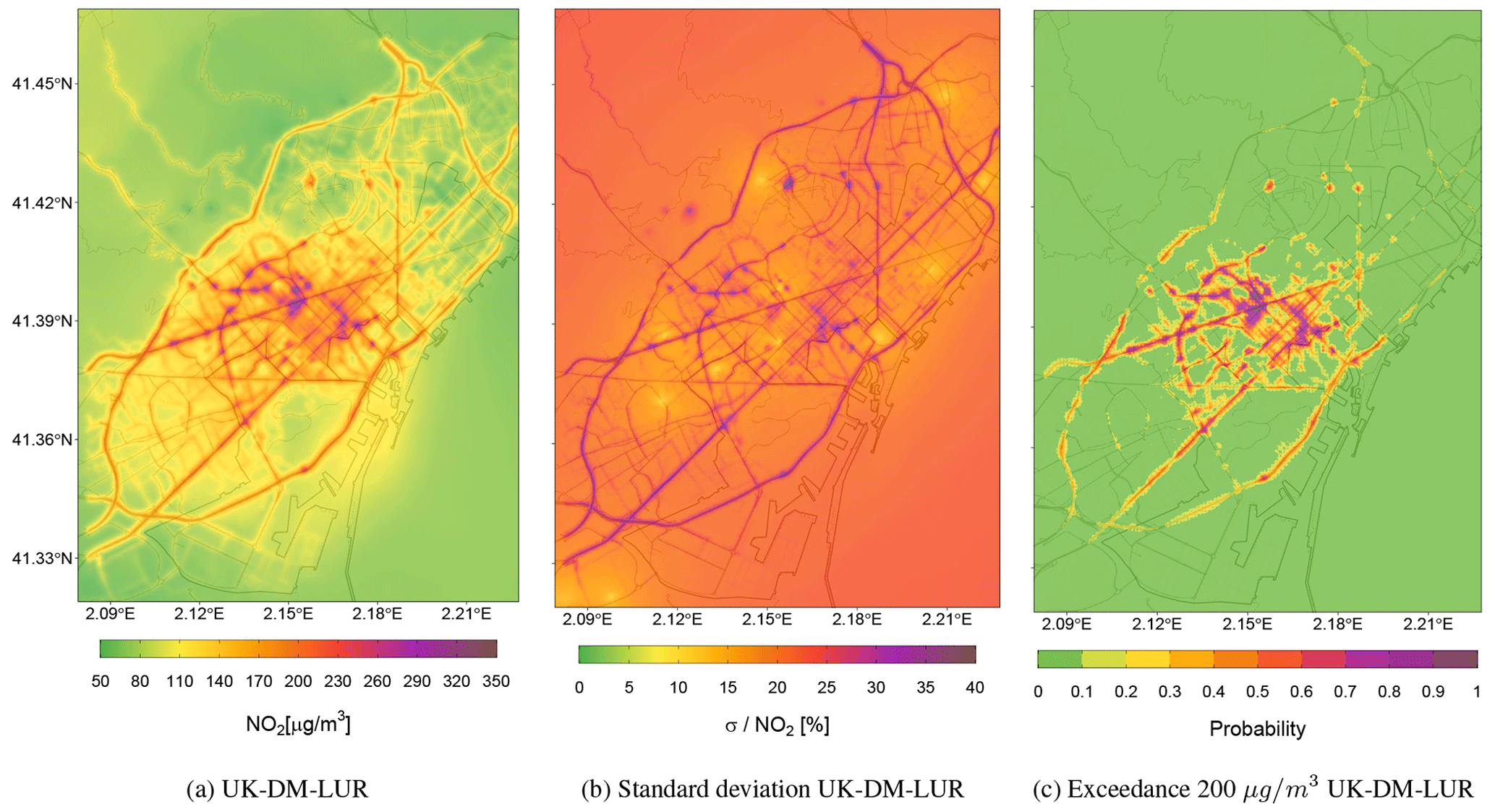
Figure 11 (a) Hourly NO₂ concentration map as a result of applying the UK-DM-LUR methodology at 09:00 UTC on 28 February 2019. (b) Relative uncertainty associated with the predictions in panel (a). (c) Hourly probability map exceeding the 200 µg m⁻³ NO₂ hourly averaged limit, using the values in panels (a) and (b).

Figure 11 presents the NO₂ prediction at a specific hour, its associated relative uncertainty, and the exceedance probability map based on the 200 µg m⁻³ NO₂ hourly threshold (AAQD 2008/EC/50) for the UK-DM-LUR methodology. The goal is to illustrate that, apart from studying the long-term NO₂ values, the present methodology can also be used to correct short NO₂ exposure episodes, such as the ones observed during traffic rush hours. Figure 11 corresponds to the peak traffic hour at 09:00 UTC on 28 February 2019, which was a particularly polluted hour, reporting 138 and 201 µg m⁻³ at the traffic monitoring stations of Eixample and Gràcia, respectively. Similar to Fig. 10, low-uncertainty regions are obtained around the locations of the monitoring stations. Likewise, high relative uncertainty regions are associated with pollution hotspots due to the extrapolation effect in the regression step. Concerning the exceedance probability maps shown in Fig. 11c, the city center and its major trafficked streets have the highest values (>0.7). In the Eixample district, 19 % of the area exceeds the NO₂ hourly limit, with a probability equal to or higher than 0.5 and 6 % in the case of 0.7.

4 Conclusions

The present work assesses the added value of including a microscale LUR basemap into a data fusion method to obtain spatially bias-corrected urban maps of NO₂ at the hourly scale. To do so, we have compared two different data fusion methods, namely (i) merging an urban dispersion model with the observational data coming from 12 monitoring stations, using universal kriging (UK-DM), and (ii) adding a nonlinear microscale LUR model as a covariate in the kriging workflow based on the GBM algorithm (UK-DM-LUR). The comparison is based on the statistical performance in LOOCV at each monitoring station, the resulting NO₂ maps, and their associated uncertainty.

The statistical performance of the microscale LUR model has been assessed using a comprehensive nested CV. As expected, the obtained microscale LUR basemap (r=0.64; RMSE=11.87 µg m⁻³) outperformed the raw annually averaged dispersion model results (r=0.54; RMSE=13.68 µg m⁻³), highlighting the convenience of using passive dosimeter campaigns to explain the spatial distribution of NO₂. Moreover, a novel traffic density variable based on the combination of different traffic buffer sizes has been shown to have a significant influence (17.7 %) in the microscale LUR basemap, suggesting its relevance in future microscale LUR models.

Adding the microscale LUR time-invariant spatial information (UK-DM-LUR) has been demonstrated to significantly improve the skills of the more straightforward data fusion UK-DM method at the hourly scale, increasing the r coefficient by 13 % and reducing the RMSE by −24 % on average over all monitoring stations during 2019. Thus, our results suggest that data fusion methods applied at the street scale benefit from high-spatial-resolution data such as passive dosimeter campaigns, urban morphology, or traffic intensity estimates. When using only monitoring stations in the data fusion approach, the spatial patterns of NO₂ mainly rely on the urban model patterns. Generally, the better the temporal and spatial coverage of observational data, the better the statistical performance that can be achieved.

To check the consistency of the estimated uncertainty, we have empirically validated the universal-kriging-based uncertainties through a LOOCV. Despite the predicted variance of the universal kriging being slightly overconfident and tending to degrade for extreme concentration values, we found that it is a meaningful estimation of uncertainty. The PDFs of the error are close to the normal distribution, especially for the UK-DM-LUR approach. The spatial characterization of the uncertainty adds value to the NO₂ concentration maps, making data fusion results more comprehensive for regulatory purposes, decision-makers, and health impact assessment. For instance, uncertainty maps can be used to allocate new observational stations or to plan future LCS campaigns. In this regard, our results show that pollution hotspots are areas of high uncertainty that are underrepresented by the current monitoring system. We thus stress the need to monitor the vicinity of heavily trafficked roads better to increase the performance of data fusion methods in predicting hourly and annual exceedances.

In developing our microscale LUR model, a limitation arises when using campaigns conducted between February and March. Although the annualization adjustment factor corrects the NO₂ values, the spatial patterns are still linked to the period of the campaigns. If additional campaigns from different seasons of the year were available, then assessing the seasonal bias effects on the spatial gradients would be highly interesting. Ideally, the basemap should be on a seasonal scale rather than a yearly scale. This highlights room for a potential improvement in our methodology because we could not quantify this in the present analysis due to the lack of experimental campaigns during other seasons of the year. Another limitation identified is that the Observatori Fabra station has been excluded from the data fusion methodology because its inclusion worsened the results in the urban environment. Although its exclusion means losing relevant information regarding low-NO₂-level areas, the primary objective of the urban model is to identify NO₂ exceedances in highly trafficked areas.

Local authorities frequently conduct air quality diagnoses based solely on available monitoring stations, resulting in inaccurate assessments of the situation, since numerous local pollution hotspots remain unmonitored. We have shown that data fusion methods can provide a more comprehensive analysis by minimizing the sampling bias. For instance, in 2019, only the Gràcia and Eixample stations exceeded the annual legal NO₂ limit of 40 µg m⁻³, and just four hourly exceedances were recorded during this period in Barcelona. In contrast, our results point out that large, built-up areas and the main transit streets in the city recurrently exceeded the legal limits during the same period. Particularly, 13 % of Barcelona has a probability of 0.7 or higher of exceeding the NO₂ annual limit value of 40 µg m⁻³, which increases to 30 % with a probability of 0.5 or higher. For the Eixample district, which is the most populous and densely populated, those percentages are 69 % and 95 %, respectively.

A strong point of the presented methodology is the characterization of the NO₂ spatial patterns by combining two sources of information, namely the urban dispersion model and the microscale LUR model. Therefore, the transferability of this method to other cities depends upon the existence of relevant passive dosimeter observations (or other observations providing constraints on the spatial variability at urban/street level) and the availability of a high-resolution urban air quality model. Regarding the urban dispersion model, key aspects are the availability of a detailed road network to derive meaningful emissions and utilizing a skilled regional model to prescribe the boundary conditions accurately. On the other hand, Appendix A presents an assessment of the necessary number of samplers to retrieve a valid microscale LUR model. On top of that, a network of monitoring stations plays a crucial role in the regression step of universal kriging, as a linear model is derived every hour. In this study, we observed that at least four monitoring stations have to be available to build robust linear regressions. However, this might vary, depending on the specificities of the analysis, such as the urban model skills and the size of the city.

Appendix A: Impact of selected passive dosimeter campaigns on the data fusion results

An assessment of the passive dosimeters data needed for the present data fusion methods is provided here. Despite the specificities of the data, this assessment is intended to aid in the transferability to other cities. First, Sect. A1 provides a statistical assessment of the data fusion techniques as a function of the experimental campaign used. Second, Sect. A2 includes a brief discussion of the number of samplers required.

A1 Impact of combining different experimental campaigns

We have calculated the effect of using campaigns from different years at two distinct levels, namely effects on the microscale LUR performance and effects on the overall data fusion workflow performance (UK-DM-LUR).

A1.1 Impact on the microscale LUR performance

Applying the performance evaluation procedure described in Sect. 3.1.1, Table A1 compares statistical results for the microscale LUR model when relying solely on data from the CSIC or the xAire campaigns. As a reference, we have also added the results of the raw CALIOPE-Urban model and the microscale LUR performance when using both campaigns (already shown in Table 2).

Table A1 Statistical results of the microscale LUR model in nested CV, considering both campaigns or only one of them. The 2017 annual mean concentration of NO₂ of the raw dispersion model (CALIOPE-Urban) is also shown.

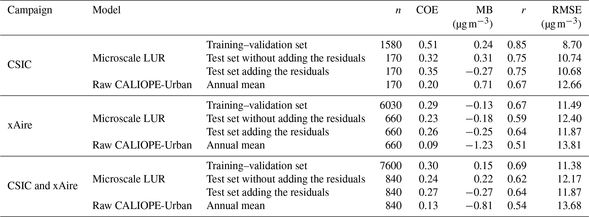
The microscale LUR model, based solely on the CSIC campaign, exhibits superior performance compared to the model based on both campaigns, whereas the model based solely on the xAire campaign demonstrates the opposite trend. However, there are notable differences in the number of data points and the motivation behind each campaign. The CSIC campaign deployed fewer samplers (175), which raises concerns about possible overfitting. In this line, the COE statistic shows a significant decline (∼40 %) between the training set and the test set without residuals, although the decrease in performance for the other statistics is not as prominent. Additionally, we expect a higher data quality from the CSIC campaign, since it was conducted by a specialized research agency. In contrast, the xAire campaign was a citizen science initiative, involving school children and their families. All of this could have affected issues such as clustering (see Fig. 3), although the number of dosimeters included here in this campaign is considerably larger (669). Combining both campaigns allows us to consider more samples, to characterize the complex NO₂ gradients in the city, while reducing potential errors associated with overfitting and clustering.

A1.2 Impact on the full data fusion workflow performance

Figure A1 shows the statistical results (COE, MB, r, and RMSE) obtained through an hourly LOOCV approach across the 12 monitoring stations. The statistical analysis compares the universal kriging technique that employs only the CALIOPE-Urban output as a covariate (UK-DM), the universal kriging technique adding the microscale LUR model resulting from combining both dosimeter campaigns (UK-DM-LUR), and the UK-DM-LUR models based only on one campaign (UK-DM-LUR CSIC and UK-DM-LUR xAire). For reference, the raw CALIOPE-Urban statistical results are also presented.

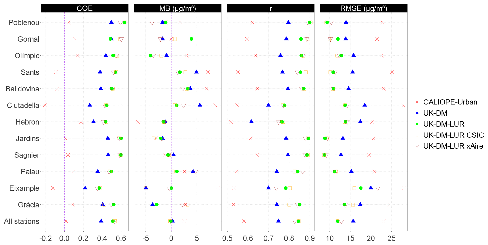
Figure A1 Statistical results for each station after applying UK-DM and UK-DM-LUR to 2019 hourly data in LOOCV. For the UK-DM-LUR application, we have considered developing the microscale LUR model with only one experimental campaign (UK-DM-LUR CSIC or UK-DM-LUR xAire) or both of them (UK-DM-LUR). In addition, we show the statistical results for the CALIOPE-Urban estimates at each station. All stations refer to the average over all stations.

Regardless of the configuration, UK-DM-LUR improves the UK-DM methodology (and, therefore, CALIOPE-Urban) for the COE, r, and RMSE indicators. For the MB indicator, there is no clear trend once again. Once the microscale LUR model was integrated into the universal kriging framework, the statistical differences among UK-DM-LUR configurations were less significant than the ones shown in Table A1. It should be noted that the LOOCV is carried out in a limited number of monitoring stations (12), which represents a significant constraint on the current statistical evaluation. Despite this limitation in the evaluation, we consider that the broader spatial coverage of the samplers when combining both campaigns is the best option because it allows us to capture a greater number of complex NO₂ structures not reproduced by CALIOPE-Urban.

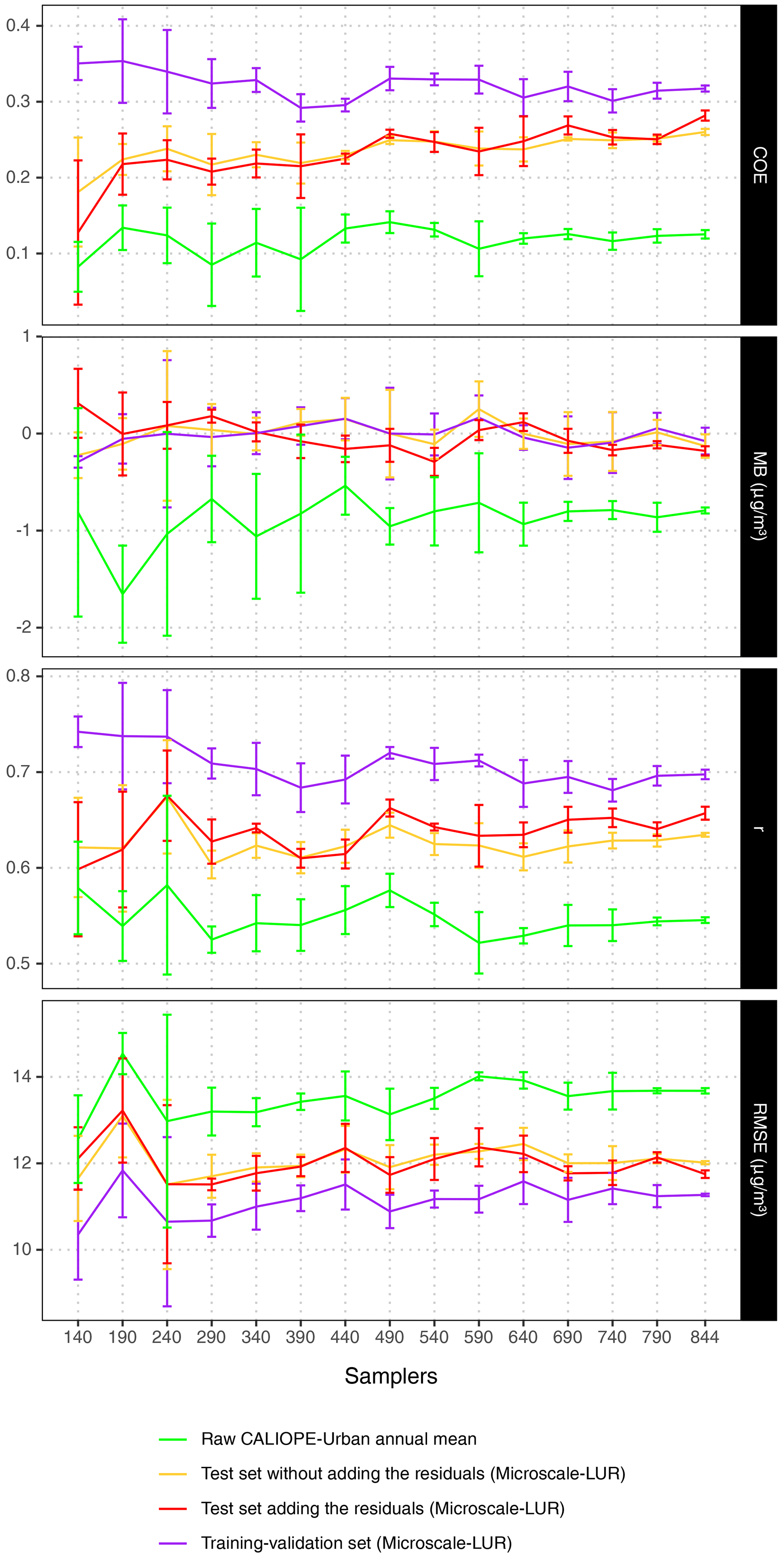
Figure A2 Statistical results of the 15 microscale LUR models in nested CVs. The models are built by considering both dosimeter campaigns and gradually increasing the number of samplers from 140 to 790 by uniform increments of 50 random samplers, in addition to the final model with all of the samplers (844). The statistics represent the evaluation of the microscale LUR models for the training and test (with and without the correction of the residuals) sets. The 2017 annual mean concentration of NO₂ of the raw dispersion model (CALIOPE-Urban) is also shown and evaluated at the locations of the dosimeters.

A2 Impact of the number of samplers considered on the microscale LUR performance

In the case of using two campaigns, we have computed the microscale LUR performance by gradually increasing the number of samplers from 140 to 790 with uniform increments of 50 random samplers, which results in 14 new models. In addition, we have also added the final model with all samplers (844) to make a comparison. To ensure the robustness of the results, we repeated these computations three times, randomly varying the selected samplers. Then, from these three series, the average and the standard deviation of the statistical indicators are computed. Figure A2 compares the COE, MB, r, and RMSE when gradually increasing the number of samplers for the training dataset, the test dataset, the test dataset interpolating the residuals, and the raw CALIOPE-Urban output.

As expected, as more samplers are considered, the standard deviation of the different metrics decreases. Also, an increasing trend in COE and r for the test sets is observed, while the same statistics decrease for the training sets. This opposite trend indicates that the overfitting is being reduced as more samplers are considered. For the test sets, the RMSE fluctuates around 12 µg m⁻³ beyond 290 samplers with a moderated variability. Despite some fluctuations in the results, we can conclude that, from the 290th sampler onwards, the COE differences between training and test sets, as well as the resulting RMSE, remain more or less constant. Therefore, based on these results, we would recommend a minimum of 290 samplers to build the microscale LUR.