4DVarNet-SSH: end-to-end learning of variational interpolation schemes for nadir and wide-swath satellite altimetry

The reconstruction of sea surface currents from satellite altimeter data is a key challenge in spatial oceanography, especially with the upcoming wide-swath SWOT (Surface Water and Ocean and Topography) altimeter mission. Operational systems, however, generally fail to retrieve mesoscale dynamics for horizontal scales below 100 km and timescales below 10 d. Here, we address this challenge through the 4DVarnet framework, an end-to-end neural scheme backed on a variational data assimilation formulation. We introduce a parameterization of the 4DVarNet scheme dedicated to the space–time interpolation of satellite altimeter data. Within an observing system simulation experiment (NATL60), we demonstrate the relevance of the proposed approach, both for nadir and nadir plus SWOT altimeter configurations for two contrasting case study regions in terms of upper ocean dynamics. We report a relative improvement with respect to the operational optimal interpolation between 30 % and 60 % in terms of the reconstruction error. Interestingly, for the nadir plus SWOT altimeter configuration, we reach resolved space–timescales below 70 km and 7 d. The code is open source to enable reproducibility and future collaborative developments. Beyond its applicability to large-scale domains, we also address the uncertainty quantification issues and generalization properties of the proposed learning setting. We discuss further future research avenues and extensions to other ocean data assimilation and space oceanography challenges.

1 Introduction

Satellite altimetry is the main data source for the observation and reconstruction of sea surface dynamics on a global scale (Chelton et al., 2001). Current satellite altimeters only deliver along-track nadir observations. This results in a very scarce sampling of the ocean surface. Interpolation schemes are then key components of the operational processing of satellite altimetry data. Current operational products (Taburet et al., 2019; Lellouche et al., 2018), however, show a limited ability to retrieve the full range of mesoscale dynamics. The upcoming wide-swath altimetry SWOT (Surface Water and Ocean and Topography) mission (see, e.g., Gaultier et al., 2015) will provide, for the first time, a two-dimensional observation of the sea surface height (SSH). The space–time sampling of satellite altimeters will, however, still remain scarce for a long time, which has motivated the recent surge in research literature towards the finding an improvement of the interpolation of satellite-derived SSH fields (see, e.g., Lopez-Radcenco et al., 2019, Lguensat et al., 2017, Beauchamp et al., 2021, and Ballarotta et al., 2019).

Besides operational schemes based on optimal interpolation techniques (Taburet et al., 2019) and data assimilation schemes for ocean circulation models (Benkiran et al., 2021), we may sort the proposed SSH interpolation schemes into three main categories, namely extension of optimal interpolation approaches towards multiscale schemes (Ardhuin et al., 2020), data assimilation schemes using sea surface dynamical priors such as quasi-geostrophic (QG) dynamics (Le Guillou et al., 2020), and data-driven interpolation methods. The latter comprises both EOF-based (empirical orthogonal function) techniques (Beckers and Rixen, 2003b; Alvera-Azcárate et al., 2009), analog approaches (Lguensat et al., 2017; Tandeo et al., 2020), and, more recently, deep learning schemes (Fablet et al., 2020; Fablet and Chapron, 2022; Manucharyan et al., 2021; Beauchamp et al., 2020).

Here, we further explore this avenue and, more specifically, the 4DVarNet framework recently introduced in Fablet et al. (2021). As it relies on a variational data assimilation formulation, it appears to be particularly suited to the space–time interpolation of sea surface variables from irregularly sampled observations. We propose a parameterization of the 4DVarNet scheme dedicated to SSH interpolation from satellite altimeter data and report OSSE (observing system simulation experiment) results to support the relevance of the proposed scheme. Our main contributions are as follows:

• The proposed 4DVarNet-SSH scheme delivers an end-to-end neural architecture using raw satellite altimeter data and optimally interpolated fields as input. We also address uncertainty quantification issues using an ensemble method.

• For the OSSE on two case study regions, respectively, along the GULFSTREAM, and for an open-ocean area dominated by mesoscale eddy dynamics, the 4DVarNet-SSH scheme outperforms previous work and significantly improves the performance metrics with respect to the operational processing. We also support the relevance of wide-swath SWOT altimeter data to significantly improve the reconstruction of sea surface dynamics compared to nadir-only satellite altimeters.

• We deliver an open-source code for the proposed 4DVarNet-SSH scheme. It relies on PyTorch and associated state-of-the-art packages. As such, it supports multi-GPU configuration and can scale up to large-scale domains.

We believe that these contributions are able to help in the development of deep learning approaches for satellite altimetry and, more broadly, for operational oceanography.

This paper is organized as follows. Section 2 briefly reviews the key methodological aspects and related work. We describe the proposed 4DVarNet-SSH approach in Sect. 3, and Sect. 4 presents the considered OSSE setting. We report our results in Sect. 5 and further discuss our main contributions in Sect. 6.

2 Background and related work

From a methodological point of view, interpolation problems in geoscience are classically regarded as data assimilation issues (Asch et al., 2016). They aim at estimating the state x_t of a multidimensional dynamical system as follows:

$$\begin{array}{}\text{(1)}& {\displaystyle }\left\{\begin{array}{ll}\frac{\mathrm{d}{\mathit{x}}_t}{\mathrm{d}t}& =\mathcal{M}\left({\mathit{x}}_t\right)+{\mathit{\eta }}_t\\ {\mathit{y}}_t& ={\mathcal{H}}_t\left({\mathit{x}}_t\right)+{\mathit{\epsilon }}_t\end{array}\right..\end{array}$$

The first equation relates to the forecast step which describes the evolution of the system from time t to t+dt, according to the potentially nonlinear model ${\mathit{x}}_{k+\mathrm{1}}=\mathcal{M}\left({\mathit{x}}_k\right)$. The second equation introduces the observations y_t at time t, where ℋ_t is the corresponding observation operator, which is usually known and also potentially learnable. η(t) is the model error and ε(t) the observation error. Both errors are generally assumed to be Gaussian, unbiased, and uncorrelated over time. When discretized on a spatiotemporal grid, where index $k=\mathrm{1},\mathrm{\cdots },T$ refers to time t_k, their associated covariance matrices are ${\mathbf{Q}}_k\in {\mathbb{R}}^{m\times m}$ and ${\mathbf{R}}_k\in {\mathbb{R}}^{p_k\times p_k}$.

Broadly speaking, a vast family of data assimilation methods stems from the minimization of some energy or function which involves two terms, a dynamical prior, and an observation term. We may distinguish two main categories of data assimilation approaches (Evensen, 2009), namely variational and statistical data assimilation. Specifically, within a variational data assimilation framework, the state analysis x^a results in a gradient-based minimization of the defined variational cost $\mathcal{J}\left(\mathit{x}\right)={\mathcal{J}}_{\mathrm{\Phi }}(\mathit{x},\mathit{y},\mathrm{\Omega })$ (Asch et al., 2016). The latter generally combines the sum of an observation term and a regularization term involving an operator Φ, as follows:

$$\begin{array}{ll}{\displaystyle }{\mathcal{J}}_{\mathrm{\Phi }}(\mathit{x},\mathit{y},\mathrm{\Omega })& {\displaystyle }={\displaystyle \frac{\mathrm{1}}{\mathrm{2}}}\sum _{i=k-L}^{k+L}\left|\right|{\mathit{y}}_i-{\mathcal{H}}_i\left({\mathit{x}}_i\right)|{|}_{{\mathbf{R}}_i^{-\mathrm{1}}}^{\mathrm{2}}\\ {\displaystyle }& {\displaystyle }+{\displaystyle \frac{\mathrm{1}}{\mathrm{2}}}\sum _{i=k-L}^{k+L}\left|\right|{\mathit{x}}_i-{\mathrm{\Phi }}_i\left({\mathit{x}}_i\right)|{|}_{{\mathbf{Q}}_i^{-\mathrm{1}}}^{\mathrm{2}}.\end{array}$$

The prior operator Φ_k is a time-stepping operator at time t_k. In a model-based data assimilation, it generally relates to a dynamical model ℳ to provide a background estimation (i.e., the physical prior) corresponding to the deterministic forecast. $\mathit{x}=\mathit{\{}{x}_{k-L},\mathrm{\cdots },x_{k+L}\mathit{\}}$, respectively, denotes the temporal vectors of sizes $(\mathrm{2}L+\mathrm{1})\times m$, and ${\prod }_{i=k-L}^{k+L}{p}_i$ associated with the state of the system and the observations within the data assimilation window (DAW) of length 2L+1 centered around t_k. ℋ_k is the observation operator, and Ω={Ω_k} is the set of subdomains of 𝒟, with observations at times t_k, $k=\mathrm{1},\mathrm{\cdots },T$. Last, Q_k and R_k are the background and the observation error covariance matrices. This formulation of functional ${\mathcal{J}}_{\mathrm{\Phi }}(\mathit{x},\mathit{y},\mathrm{\Omega })$ directly relates to weak constraint 4D-Var (see, e.g., Carrassi et al., 2018), which aims at estimating the optimal trajectory of a system in a predefined DAW, given the additional constraint of model uncertainty in the objective function 𝒥.

Regarding statistical data assimilation, many state-of-the-art methods rely on optimal interpolation (OI), which is the basic block of all statistical methods, especially regarding SSH-related datasets. OI has been used for decades (Taburet et al., 2019) for the interpolation of along-track nadir altimeter datasets and is still used today for the operational marine (Copernicus Marine Environment Monitoring Service, CMEMS) and climate (Copernicus Climate Change Service, C3S) production of the EU Copernicus program. It involves a significant smoothing for solving spatial scales up to 150 km. Extensions of OI schemes to multiscales to better account for mesoscale sea surface dynamics have recently been proposed (Ardhuin et al., 2020; Ubelmann et al., 2016).

Variational DA schemes have also been widely explored for the assimilation of satellite altimeter data in ocean general circulation models (see, e.g., Ngodock et al., 2015, Benkiran et al., 2021, or Li et al., 2021). Previous works have also considered quasi-geostrophic (QG) dynamics as an approximate and reduced-order dynamical prior for sea surface dynamics, leading to state-of-the-art performance (Ubelmann et al., 2016; Le Guillou et al., 2020).

Whereas model-driven and optimal interpolation approaches are the state-of-the-art solutions for operational products, data-driven strategies have recently emerged as promising alternatives to improve the space–time resolution of interpolated products. We may cite, among others, DINEOF (Data Interpolating Empirical Orthogonal Functions; Beckers and Rixen, 2003a; Alvera-Azcárate et al., 2005, 2009) and the analog data assimilation (AnDA; Lguensat et al., 2017; Tandeo et al., 2020) and the recent developments of deep learning schemes (Barth et al., 2019). Beauchamp et al. (2020) have reported a benchmarking experiment, which supported the relevance of data-driven schemes compared with the operational OI product.

Here, we further explore deep learning approaches, and more particularly the 4DVarNet scheme (Fablet and Chapron, 2022), which bridges variational data assimilation and deep learning. Because the analyzed state obtained from OI matches the minimization of the 3D-Var cost function, this establishes the formal link between the statistical DA framework and the optimal control theory used in the variational formulation. When adding time as an extra dimension, 4D-Var generalizes the stationary case of the 3D-Var formulation (see, e.g., Carrassi et al., 2018). It makes the 4DVarNet framework relevant for comparison with traditional DA methods. The BOOST-SWOT 2020 data challenge (https://github.com/ocean-data-challenges/2020a_SSH_mapping_NATL60, last access: 2022) provides a representative benchmarking framework to assess the performance of SSH mapping schemes for nadir-only and nadir plus SWOT (denoted as nadir+swot in the figures) altimetry datasets.

As detailed hereafter, we introduce a parameterization of the 4DVarNet scheme dedicated to SSH interpolation issues and demonstrate its relevance in the context of the benchmarking settings introduced in the BOOST-SWOT 2020 data challenge.

3 Method

This section details the proposed learning-based framework for the interpolation of satellite altimeter data. We first briefly review 4DVarNet framework recently introduced in Fablet et al. (2021) in Sect. 3.1 and present the proposed parameterization for SSH mapping from nadir and SWOT altimeter data in Sect. 3.2. We describe the resulting PyTorch package and its associated implementation details in Sect. 3.4 and the proposed learning setting in Sect. 3.3.

3.1 4DVarNet framework

The 4DVarNet framework introduced in Fablet et al. (2021) provides a generic approach for the training of 4D-Var models and solvers. They have been shown to outperform classic 4D-Var solvers for toy case studies, such as Lorenz-63 and Lorenz-96 dynamics, when considering partially observed systems. The 4DVarNet framework can be regarded as an extension that used trainable, gradient-based solvers of the deep learning scheme, which led to the best SSH interpolation performance in our previous work (Beauchamp et al., 2020).

From a methodological point of view, the 4DVarNet framework derives an end-to-end neural architecture from an underlying variational data assimilation (DA) formulation (see Sect. 2 again) as follows:

$$\begin{array}{}\text{(2)}& {\displaystyle }{\mathcal{J}}_{\mathrm{\Phi }}(\mathit{x},\mathit{y},\mathrm{\Omega }){\displaystyle }={\mathit{\lambda }}_{\mathrm{1}}\left|\right|\mathit{y}-\mathcal{H}\left(\mathit{x}\right)|{|}_{\mathrm{\Omega }}^{\mathrm{2}}+{\mathit{\lambda }}_{\mathrm{2}}||\mathit{x}-\mathrm{\Phi }(\mathit{x}\left)\right|{|}^{\mathrm{2}},\end{array}$$

where λ_1,2 are predefined or tunable scalar weights, and we replaced the Mahalanobis norms $\left|\right|.|{|}_R^{-\mathrm{1}}$ and $\left|\right|.|{|}_Q^{-\mathrm{1}}$ with a standard mean square norm for the sake of simplicity. In the regularization term, we substitute the traditional dynamical prior ℳ with a neural operator Φ based on a convolutional architecture. Then, we can exploit the automatic differentiation tools embedded in deep learning libraries to consider the following iterative gradient-based solver, denoted as Γ, for the minimization of variational cost 𝒥_Φ with regard to the state x, as follows:

$$\begin{array}{}\text{(3)}& \left\{\begin{array}{cl}{g}^{(i+\mathrm{1})}& =\mathrm{LSTM}\left[\mathit{\alpha }\cdot {\mathrm{\nabla }}_{\mathit{x}}{\mathcal{J}}_{\mathrm{\Phi }}({\mathit{x}}^{\left(i\right)},\mathit{y},\mathrm{\Omega }),h\left(i\right),c\left(i\right)\right]\\ & \\ x^{(i+\mathrm{1})}& =x^{\left(i\right)}-\mathcal{T}\left(g^{(i+\mathrm{1})}\right)\end{array},\right.\end{array}$$

where LSTM denotes a convolutional long short-term memory model (see, e.g., Shi et al., 2015), α a is normalization scalar, h(i) and c(i) denote the internal states of the LSTM, and 𝒯 is a linear mapping. The key idea relies on the capability of the LSTM to learn an adaptive gradient update g⁽ⁱ⁺¹⁾ from the gradient of the variational cost ∇_x𝒥_Φ(x⁽ⁱ⁾) in order to considerably speed up the optimization and reach the corresponding optimal state. This iterative rule, based on a trainable LSTM operator, is similar to meta-learning schemes (Andrychowicz et al., 2016). Due to the ability of LSTM models to capture long-term dependencies, it results in a trainable gradient descent with momentum.

Figure 1 Sketch of the gradient-based algorithm. The upper-left stack of images corresponds to an example of the temporal sequence of SSH observations, with missing data used as input. The upper-right stack of images is an example of intermediate reconstruction of the SSH gradient at iteration i, while the bottom-left stack of images identifies the updated reconstruction fields used as new inputs after each iteration of the algorithm.

Overall, a 4DVarNet scheme defines a neural architecture which runs a predefined number of iterative gradient-based updates (see Eq. 3). Let us denote ${\mathrm{\Psi }}_{\mathrm{\Phi },\mathrm{\Gamma }}({\mathit{x}}^{\left(\mathrm{0}\right)},\mathit{y},\mathrm{\Omega })$ as the output of the 4DVarNet architecture for a given prior Φ and solver Γ, the initialization x⁽⁰⁾ of the state x, and the observations y on the domain Ω. The resulting neural architecture is referred as an end-to-end architecture, since it uses as input raw observation data and an initial guess and directly provides as output the reconstructed state.

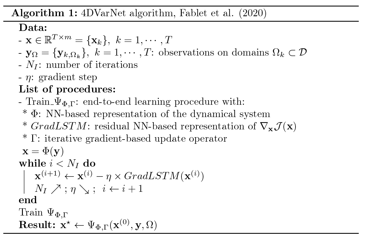
Then, the joint training of operators {Φ,Γ} is stated as the minimization of a reconstruction cost $\mathcal{L}(\mathit{x},{\mathit{x}}^{\star })$, which is typically the root mean squared error (RMSE) between the true state x and its reconstruction x^⋆ and additional regularization terms (fully described in Sect. 3.3), as follows:

$$\begin{array}{}\text{(4)}& \arg \underset{\mathrm{\Phi },\mathrm{\Gamma }}{min}\mathcal{L}(\mathit{x},{\mathit{x}}^{\star })\text{subject to}{\mathit{x}}^{\star }={\mathrm{\Psi }}_{\mathrm{\Phi },\mathrm{\Gamma }}({\mathit{x}}^{\left(\mathrm{0}\right)},\mathit{y},\mathrm{\Omega }).\end{array}$$

Let us stress that the outer loss function ℒ differs from the inner variational cost 𝒥_Φ in order to take advantage of a supervised configuration (true states are known during training). Such a formulation turns out to be particularly efficient when applied to Gaussian processes for which the optimal solution is known (see, e.g., Beauchamp et al., 2022), with promising transfer to non-Gaussian/nonlinear dynamics.

In Appendix A, a parameter-free fixed point version of the solver is also given, based on the previous results of (Beauchamp et al., 2020). In addition, Beauchamp et al. (2021) have already shown how the iterative gradient-based update is more efficient than the simpler fixed-point formulation.

3.2 4DVarNet-SSH parameterization

The proposed 4DVarNet-SSH framework aims at exploiting and improving the mapping performance of current operational OI products. This section draws from the generic 4DVarNet formulation presented above and adapts its target components, given that OI products retrieve consistent large-scale dynamics. Then, we rely on the following multiscale decomposition:

$$\begin{array}{}\text{(5)}& {\displaystyle }\mathit{x}=\stackrel{\mathrm{‾}}{\mathit{x}}+\mathrm{d}\mathit{x}+\mathit{ϵ},\end{array}$$

where the anomaly dx is seen as the difference between the true state x and the large-scale components $\stackrel{\mathrm{‾}}{\mathit{x}}$. Regarding the observation data, let us denote by y(Ω)={y_k(Ω_k)} the partial and potentially noisy altimetry observations associated with masks $\mathrm{\Omega }=\mathit{\left\{}{\mathrm{\Omega }}_k\mathit{\right\}}\subset \mathcal{D}$, where $\stackrel{\mathrm{‾}}{{\mathrm{\Omega }}_k}$ corresponds to the gappy part of the field and index k refers to time t_k. We use the operational OI product as a gap-free observation data, denoted as $\stackrel{\mathrm{‾}}{\mathit{y}}$, for the state component $\stackrel{\mathrm{‾}}{\mathit{x}}$, whereas the observation data for anomaly dx are $\mathit{y}-\stackrel{\mathrm{‾}}{\mathit{y}}$ over domain Ω.

Numerical experiments showed that an augmented-state formulation led to better interpolation performance regarding the potential stripping of artifacts due to the nadir along-track sampling. This results in the application of 4DVarNet model (see Eq. 4) to augmented states $\stackrel{\mathrm{̃}}{\mathit{x}}$ and observations $\stackrel{\mathrm{̃}}{\mathit{y}}$ are defined as follows:

$$\begin{array}{}\text{(6)}& {\displaystyle }\stackrel{\mathrm{̃}}{\mathit{x}}=\left(\begin{array}{c}\stackrel{\mathrm{‾}}{\mathit{x}}\\ \mathrm{d}{\mathit{x}}_{\mathrm{1}}\\ \mathrm{d}{\mathit{x}}_{\mathrm{2}}\end{array}\right),\stackrel{\mathrm{̃}}{\mathit{y}}=\left(\begin{array}{c}\stackrel{\mathrm{‾}}{\mathit{y}}\\ \mathrm{d}{\mathit{y}}_{\mathrm{1}}\\ \mathrm{d}{\mathit{y}}_{\mathrm{2}}\end{array}\right),\stackrel{\mathrm{̃}}{\mathrm{\Omega }}=\left(\begin{array}{c}\mathbb{1}\\ \mathrm{\Omega }\\ \mathbf{0}.\end{array}\right)\end{array}$$

This augmented-state parameterization introduces two anomaly components, dx₁ and dx₂, with corresponding observations. While only the first one is actually observed, the reconstructed SSH state is, however, given by the addition of the coarse component $\stackrel{\mathrm{‾}}{\mathit{x}}$ and the latent anomaly dx₂, where ${\mathit{x}}^{\star }=\stackrel{\mathrm{‾}}{\mathit{x}}+\mathrm{d}{\mathit{x}}_{\mathrm{2}}$.

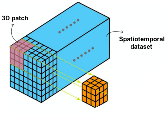
Figure 2 Patch-based strategy, where the whole spatiotemporal dataset is split into small patches. The temporal size of the patches corresponds to the length of the data assimilation window.

Following Fablet et al. (2021), the operator Φ follows a purely data-driven parameterization with two-scale residual architectures involving bilinear units (Fablet et al., 2020). The number of residual blocks is set to two, and the bilinear units are made of two hidden convolutional layers, respectively, with linear and rectified linear unit (ReLU) activations, followed by a linear scheme combining the outputs of the second layer. A final convolutional layer with linear activation is involved to bring the outputs back to the initial-state dimension. In its current implementation, Φ contains about 500 000 parameters. In any case, the number of gradient iterations for the solver Γ is fixed at five. Complementary tests showed that a higher number of iterations leads to a large increase in the training time (because of the implicit number of parameters which grows linearly with this number of iterations) without a significant gain in terms of the 4DVarNet reconstruction skills.

Regarding the initial state for iterative gradient-based rule (Eq. 3), we consider the OI field $\stackrel{\mathrm{‾}}{\mathit{y}}$ for the state component $\stackrel{\mathrm{‾}}{\mathit{x}}$, $\mathit{y}-\stackrel{\mathrm{‾}}{\mathit{y}}$ for the anomaly component dx₁, and a zero state for the anomaly component dx₂. For anomaly component dx₁, gaps are initialized to 0.

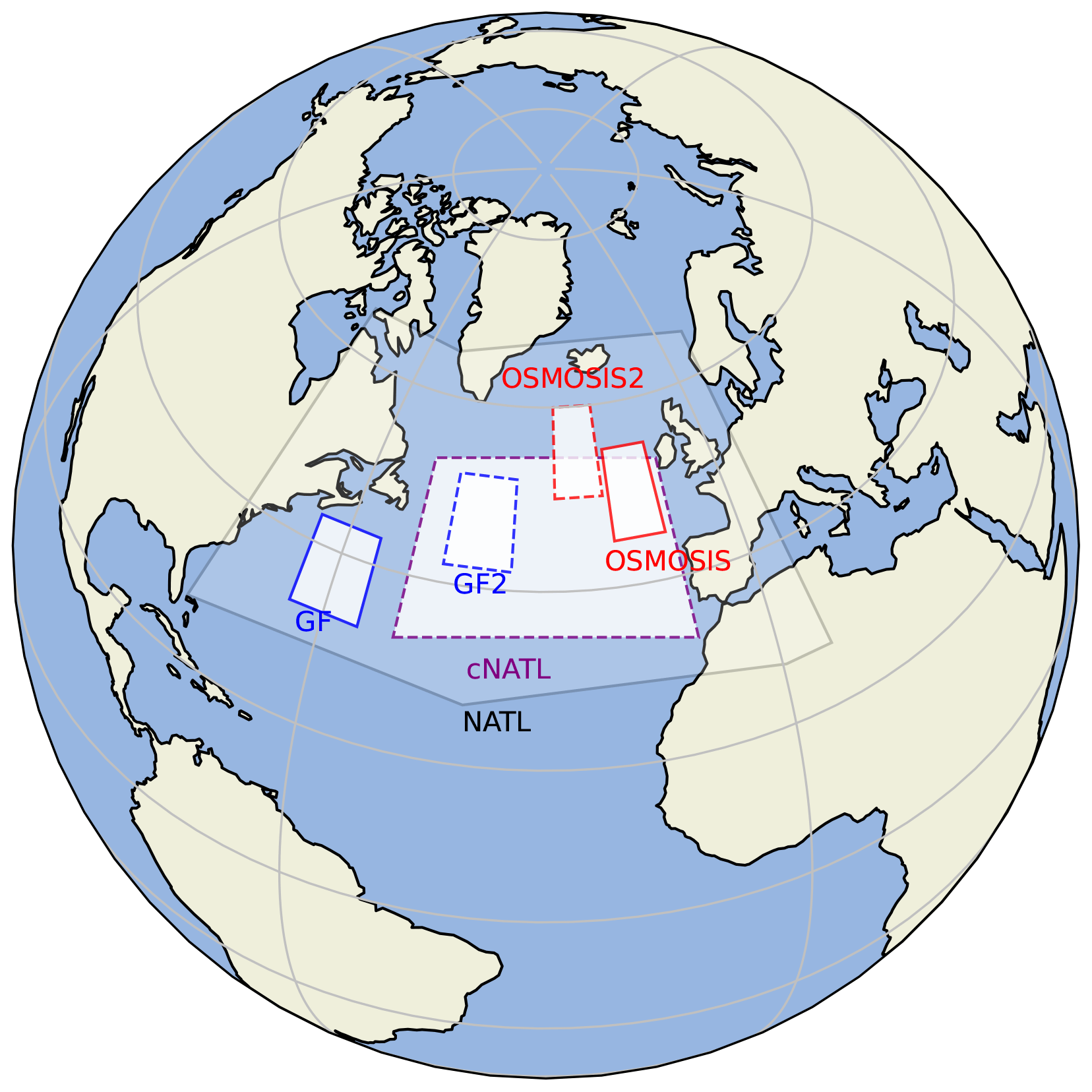
Figure 3 Extents of the GULFSTREAM, GULFSTREAM2, OSMOSIS, OSMOSIS2, and cNATL domains used in this work, which are all part of the North Atlantic (NATL) basin used in the BOOST-SWOT data challenge.

3.3 Learning setting

We implement a classic supervised learning strategy using gap-free targets. The considered training loss ℒ combines reconstruction losses and additional regularization terms as follows:

$$\begin{array}{}\text{(7)}& {\displaystyle }\mathcal{L}(\mathit{x},{\mathit{x}}^{\star })={\mathit{\lambda }}_{\mathrm{1}}\sum _{i=\mathrm{1}}^N{\mathit{w}}_i\left|\right|\mathit{x}-{\mathit{x}}^{\star }|{|}^{\mathrm{2}}+{\mathit{\lambda }}_{\mathrm{2}}|\sum _{i=\mathrm{1}}^N{\mathit{w}}_i|{\mathrm{\nabla }}_{\mathit{x}}-{\mathrm{\nabla }}_{{\mathit{x}}^{\star }}|{|}^{\mathrm{2}}\text{(8)}& {\displaystyle }+{\mathit{\lambda }}_{\mathrm{3}}\sum _{i=\mathrm{1}}^N{\mathit{w}}_i\left|\right|\mathit{x}-\mathrm{\Phi }\left({\mathit{x}}^{\star }\right)|{|}^{\mathrm{2}}+{\mathit{\lambda }}_{\mathrm{4}}\sum _{i=\mathrm{1}}^N{\mathit{w}}_i||\mathit{x}-\mathrm{\Phi }(\mathit{x}\left)\right|{|}^{\mathrm{2}},\end{array}$$

i.e., the L2 norm of the difference between the state x and reconstruction x^⋆, in addition to their gradients, and regularization losses according to the prior Φ is to enforce that both the true states and the reconstructed ones are correctly encoded by prior Φ. w={w_i}, $i=\mathrm{1},\mathrm{\cdots },N$ denote a weighting vector along the data assimilation window of size N (=7 here). To give more importance to the center of the DAW, we use the following:

$$\begin{array}{}\text{(9)}& {\displaystyle }\mathit{w}={\left[\begin{array}{ccccccc}\mathrm{0}& \mathrm{0.25}& \mathrm{0.75}& \mathrm{1}& \mathrm{0.75}& \mathrm{0.25}& \mathrm{0}\end{array}\right]}^{\mathrm{T}}.\end{array}$$

This training loss is used in Sect. 4 for the OSSE-based BOOST-SWOT data challenge framework.

Regarding the training configuration, when the domain is small (see the GULFSTREAM and OSMOSIS regions defined in Sect. 4), we use a single GPU and Adam optimizer with a batch size of 2 over 200 epochs. The same set of parameters holds for larger domains (NATL and cNATL; see again Table 1), but we use the 4DVarNet-distributed version of the code over 4 GPUs. The computational time of the training procedure lies between 4 and 5 h for the small-domain setup and between 7 and 8 h for the large-domain setup.

3.4 Implementation aspects

We provide an open-source PyTorch implementation of the 4DVarNet-SSH scheme. (The code is available at https://doi.org/10.5281/zenodo.7186322, hgeorgenthum et al., 2023). PyTorch is a state-of-the-art deep learning framework. We benefit from the associated packages such as lightning and hydra to provide a high-level environment and make the reproduction of the experiments and the development of other applications easier. Through the lightning package, our implementation supports multi-GPU distributed learning configurations. This may be highly relevant for speeding up the training process.

Regarding computational issues, the OSSE-based applications (see Sect. 4) involve the processing of $\mathrm{7}\times \mathrm{240}\times \mathrm{240}$ tensors (i.e., 7 d time series over a $\mathrm{12}{}^{\circ }\times \mathrm{12}{}^{\circ }$ domain with a $\mathrm{1}/\mathrm{20}{}^{\circ }$ resolution). GPUs with a significant RAM (typically above 30 Gb), such as NVIDIA V100, A40, and A100, can process such tensors through the proposed 4DVarNet architecture. The direct training 4DVarNet models over larger spatial domains is, however, limited by the GPU memory. To address this issue, we develop a specific data management module, through so-called data loaders. Our data loader module automatically extracts patches of a predefined size (typically, $\mathrm{7}\times \mathrm{240}\times \mathrm{240}$ in the reported experiments) from the considered training dataset according to stride parameters (as sketched in Fig. 2). One can exploit the same approach to apply a learned model to a large domain during the evaluation or production stage. In both cases, we benefit from the fully convolutional feature of the considered neural architecture. This guarantees that, up to border effects, the 4DVarNet processing is translation invariant.

Let us specify that the size of the tensors relates to the maximal space–time distance with significant autocorrelation of the SSH. Then, we use a data assimilation window of length $N=\mathrm{2}L+\mathrm{1}$, meaning that we use temporal sequences of the state space ${\mathit{x}}_{k\pm L}={\mathit{x}}_{k-L:k+L}$. The idea is to optimize the results for the time t_k at the center of the window $[t_{k-L};t_{k+L}]$, and the value of N has to be chosen according to the dynamics of the geophysical field considered, which is the SSH here. In the following experiments, we use a value of N=7, which seems to be enough to describe the spatiotemporal correlations of the anomaly between the ground truth and the DUACS (Data Unification and Altimeter Combination System) OI scheme. To apply 4DVarNet directly on the SSH dataset, without providing the DUACS OI baseline as a coarse version of the reconstruction, the value of N shall increase up to ∼20 d (see, e.g., Beauchamp et al., 2022). In the same vein, the spatial size of the patches is 240 × 240 pixels, with a corresponding 0.05^∘ resolution, where 12^∘ is large enough to consider the spatial autocorrelation as negligible outside of the patch.

4 Observation system simulation experiments

This section details the experimental setup considered in this study for the quantitative evaluation of the proposed framework. We first introduce the simulation dataset used in our experiments as well as the case study regions. Section 4.2 reviews the simulation satellite altimetry datasets and Sect. 4.3 describes our evaluation framework.

4.1 NATL60 dataset and case study regions

In our study, the nature run (NR) corresponds to the NATL60 configuration (Molines, 2018) of the NEMO (Nucleus for European Modelling of the Ocean) model. It is one of the most advanced, state-of-the-art, basin-scale, high-resolution ($\mathrm{1}/\mathrm{60}{}^{\circ }$) simulations available today, whose surface field effective resolution is about 7 km.

Table 1 Description of the NATL subdomains used for assessing 4DVarNet capabilities generalization.

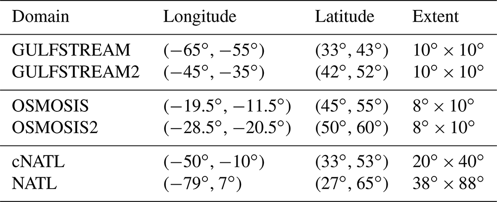
In this work, we will use the following five different subdomains of the North Atlantic basin (see Fig. 3):

• two ${\mathrm{10}}^{\circ }\times {\mathrm{10}}^{\circ }$ GULFSTREAM and GULFSTREAM2 domains,

• two ${\mathrm{8}}^{\circ }\times {\mathrm{10}}^{\circ }$ OSMOSIS and OSMOSIS2 open-ocean domains, and

• a large ${\mathrm{20}}^{\circ }\times {\mathrm{40}}^{\circ }$ cNATL domain, at the center North Atlantic basin, used to assess 4DVarNet training on large domains, without any areas of land inside to avoid any issues in the learning process.

The GULFSTREAM and OSMOSIS domains (solid blue and red lines in Fig. 3) are the domains used by the BOOST-SWOT project in the framework of the NATL60 OSSE throughout the different related studies (see their 2020 ocean data challenges in Le Guillou et al., 2020). Because we aim at exploring the capabilities of 4DVarNet to deploy at the basin scale, we also propose the two alternate GULFSTREAM2 and OSMOSIS2 domains (dashed blue and red lines in Fig. 3), with similar dynamical properties to the two initial domains, and a larger domain centered in the North Atlantic basin (cNATL; dashed purple lines). The full extent of the subdomains is summarized in Table 1.

Figure 4 NATL60 ground truth (a) and its gradient (b). Panel (c) shows 1 d accumulated along-track four nadirs, and wide-swath SSH pseudo-observations plus four nadirs are shown in panel (d), both for 25 October 2012 (GULFSTREAM domain).

Figure 5 NATL60 ground truth (a) and its gradient (b). Panel (c) shows 1 d accumulated along-track four nadirs, and wide-swath SSH pseudo-observations plus four nadirs are shown in panel (d), both for 25 October 2012 (OSMOSIS domain).

The GULFSTREAM regions display physical processes 100 times more energetic at scales larger than 100 km, with a greater temporal variability than the OSMOSIS regions. As a consequence, the SSH spatial gradient at scales above 100 km is lower for OSMOSIS regions, which explains why we can see more small-scale-related structures on such domains. In addition to their intrinsic differences in terms of the dynamical regimes, the latitudes of GULFSTREAM-based and OSMOSIS-based regions implies different SWOT temporal samplings. For OSMOSIS regions, one SWOT observation is available every day, while over the low-latitude GULFSTREAM domains, the SWOT sampling is irregular, leading to sequences of several days with only pseudo-nadir observations.

Over these regions, the SSH resolution of the nature run is downgraded to $\mathrm{1}/\mathrm{20}{}^{\circ }$, which is enough to capture both mesoscale dynamical regimes and the OSMOSIS-related smaller scales, while avoiding unnecessary heavy computation time.

The NATL60 nature run will then be used as the reference ground truth (GT) in an observing system simulation experiments (OSSEs). The pseudo-altimetric nadir and SWOT observational datasets will be generated by a realistic sub-sampling of satellite constellations.

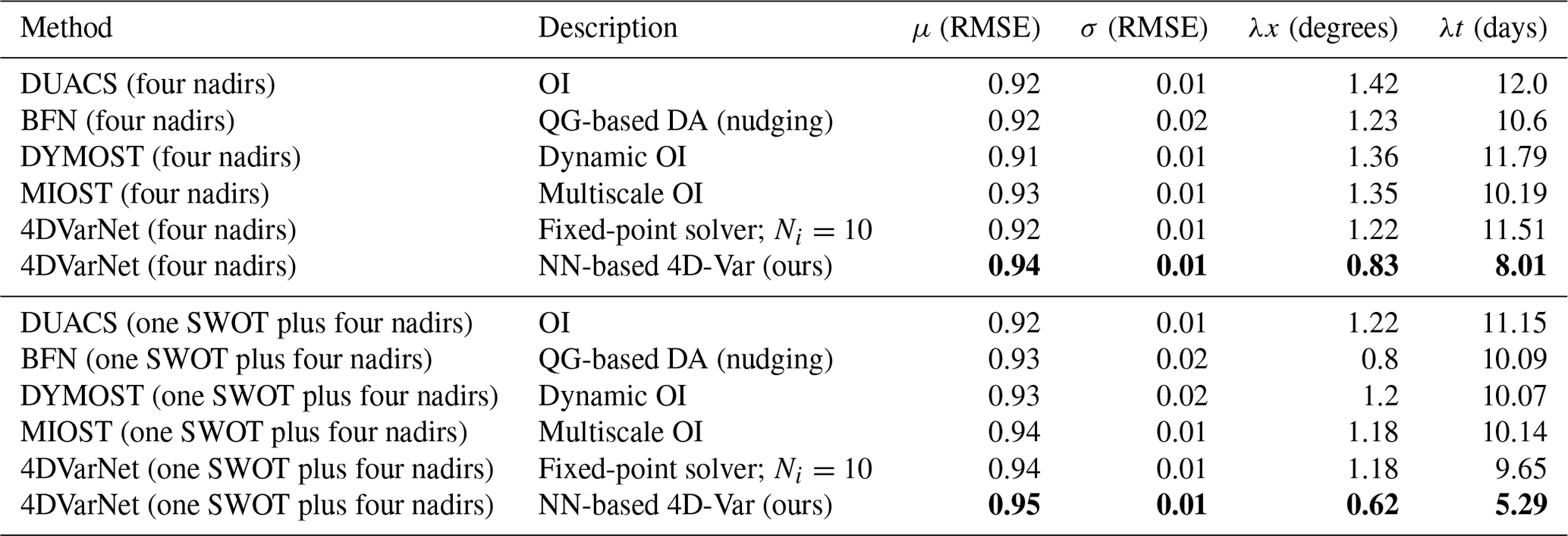
Table 2 4DVarNet-SSH performance on the GULFSTREAM domain compared to DUACS OI (traditional covariance-based optimal interpolation), BFN (back-and-forth nudging of a QG model), MIOST (multiscale OI), DYMOST (dynamic OI accounting for nonlinear temporal propagation of the SSH fields), fixed-point versions with 10, and a single iteration of the 4DVarNet solver, over the period from 22 October to 2 December 2012 (42 d). Bold formatting stands for the best metrics.

4.2 Simulated altimetry datasets

In this section, we provide a technical description of the two observational datasets used to train 4DVarNet, namely the four nadir and one SWOT plus four nadir configurations. Regarding the pseudo-nadir altimetry dataset, representative of the current pre-SWOT observational altimetric dataset, we use the ground tracks of four altimetric missions (TOPEX/Poseidon, Geosat, Jason-1, and Envisat) picked up from the 2003 constellation to interpolate the NATL60 simulation from 1 October 2012 to 29 September 2013. A Gaussian white noise, with variance σ²=(4⋯9) cm², is added to the interpolated NATL60 simulation by the SWOT simulator tool to mimic noise with a spectrum of error consistent with global estimates from the Jason-2 altimeter (Dufau et al., 2016). We aggregate the nadir pseudo-observations on a daily basis to procure the gappy daily fields used as input by 4DVarNet-SSH. Figures 4c vs. d and Figs. 5c vs. d illustrate the resulting nadir altimetry data on 25 October 2012.

Table 3 4DVarNet-SSH performance on the OSMOSIS domain compared to DUACS OI over the period from 22 October to 2 December 2012 (42 d). Bold formatting stands for the best metrics.

We proceed similarly to simulate the SWOT pseudo-observations using the SWOT simulator tool (Gaultier et al., 2015) in its swath mode, with an along-track and across-track 2 km spatial resolution (the same theoretical resolution that the upcoming SWOT-mission-derived products are expected to provide). Let us note that we consider error-free SWOT pseudo-observations.

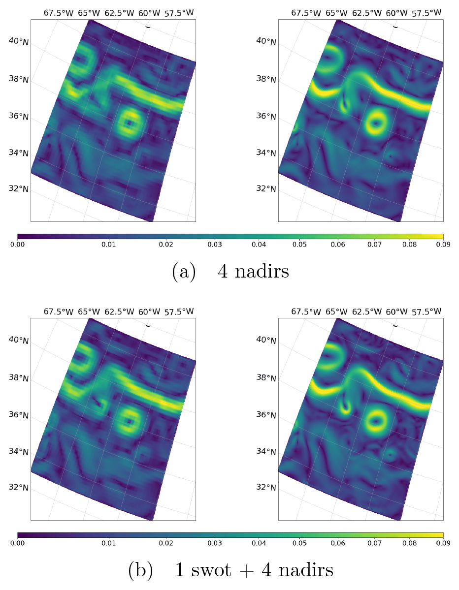
Figure 6 SSH Gradient (DUACS OI and 4DVarNet reconstruction) on 25 October 2012 for the GULFSTREAM domain.

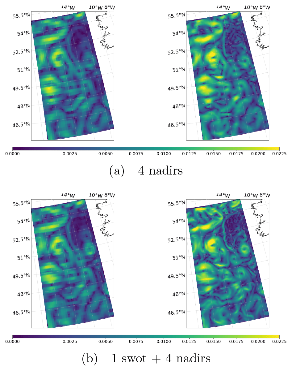
Figure 7 SSH Gradient (DUACS OI and 4DVarNet-SSH reconstruction) on 25 October 2012 for the OSMOSIS domain.

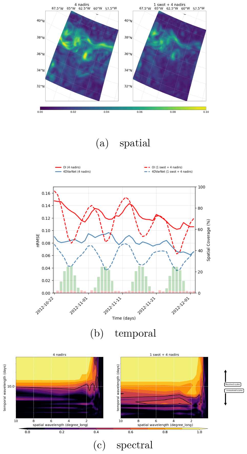
Figure 8 (a) Spatial performance, where the RMSE time series are computed for each spatial position of the GULFSTREAM domain (four nadirs on the left and one SWOT plus four nadirs on the right). (b) Temporal performance, where the RMSE daily GULFSTREAM maps are computed along the BOOST-SWOT DC evaluation period (four nadirs on the left and one SWOT plus four nadirs on the right), and the daily spatial coverage of the two configurations are given as complementary red and green bar plots scaled on the right-hand side. (c) Spectral performance, where the PSD-based score evaluates the spatiotemporal scales resolved in GULFSTREAM mapping (yellow area; four nadirs at the top and one SWOT plus four nadirs at the bottom).

4.3 Evaluation framework

Our evaluation framework exploits and extends the one introduced in Le Guillou et al. (2020), as follows:

• Training and evaluation setting. Because the NATL60 dataset is made of 365 daily simulations, and the reference data used for training never have to be used during the optimization, we train all learning-based models using the time period from 4 February to 30 September 2013. During the training procedure, we select the best model according to the metrics computed over the validation period from 1 January to 2 February 2013. Overall, we evaluate the performance metrics over the test period from 22 October to 2 December 2012, which is 42 d, corresponding to two SWOT cycles in the SWOT science-phase orbit. In doing so, the test period can be considered uncorrelated to the training and validation period.

• Evaluation metrics. We use BOOST-SWOT DC (data challenge) metrics to benchmark the 4DVarNet-SSH scheme with respect to the state-of-the-art SSH interpolation schemes. They comprise the following:

  • –

    $\stackrel{\mathrm{‾}}{{\mathrm{RMSE}}_{\mathrm{s}}\left(t\right)}$, for the mean RMSE score (normalized RMSE),

  • –

    σ[RMSE_s(t)], for the RMSE(t) standard deviation of the RMSE(t), which gives some information regarding the temporal stability of the reconstruction,

  • –

    λ_x, for which the minimum spatial scale is resolved (wavelength in degrees),

  • –

    λ_t, for which the minimum temporal scale is resolved (wavelength in days),

  where ${\mathrm{RMSE}}_{\mathrm{s}}\left(t\right)=\mathrm{1}-\frac{\mathrm{RMSE}\left(t\right)}{\mathrm{RMS}\left(\mathit{x}\right)}$, RMS denotes the root mean square function, N is the number of pixels included in the study domain, and $\mathrm{RMSE}\left(t\right)=\sqrt{\frac{\mathrm{1}}{N}{\sum }_{i=\mathrm{1}}^N\left({\mathit{x}}^{\star }\right(t,i)-\mathit{x}(t,i){)}^{\mathrm{2}}}$. Last, the spectral analysis (λ_x and λ_t) is based on the wavenumber frequency power spectral density score PSD${}_{\mathrm{S}}^{\mathrm{wf}}$, which is defined as PSD${}_{\mathrm{S}}^{\mathrm{wf}}=\mathrm{1}-\frac{{\mathrm{PSD}}^{\mathrm{wf}}({\mathit{x}}^{\star }-\mathit{x})}{{\mathrm{PSD}}^{\mathrm{wf}}\left(\mathit{x}\right)}$. We refer the reader to Le Guillou et al. (2020) for additional descriptions regarding these metrics. Besides these quantitative metrics, we also analyze the space–time distribution of the interpolation error and explore the impact of the interpolation for the characterization of mesoscale eddy dynamics. Based on the work of Mason et al. (2014), we detect anticyclonic and cyclonic eddies in the ground truth NATL60 outputs, interpolate SSH fields using the py-eddy-tracker toolbox (Delepoulle et al., 2022), and analyze how key features of matching eddies, such as speed radius (km), outer radius (km), amplitude (cm), and speed max (cm s⁻¹), are retrieved.

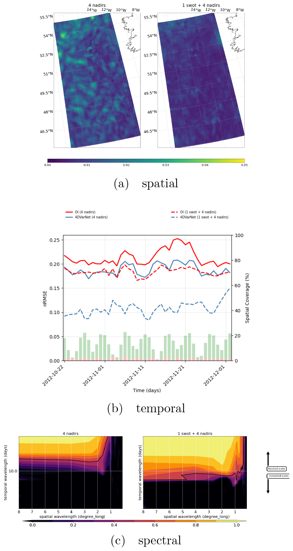
Figure 9 (a) Spatial performance, where the RMSE time series are computed for each spatial position of the GULFSTREAM domain (four nadirs on the left and one SWOT plus four nadirs on the right). (b) Temporal performance, where the RMSE daily GULFSTREAM maps are computed along the BOOST-SWOT DC evaluation period (four nadirs on the left and one SWOT plus four nadirs on the right), and the daily spatial coverage of the two configurations are given as complementary red and green bar plots scaled on the right-hand side. (c) Spectral performance, where the PSD-based score evaluates the spatiotemporal scales resolved in GULFSTREAM mapping (yellow area; four nadirs at the top and one SWOT plus four nadirs at the bottom).

5 Results

This section presents the considered OSSE for the evaluation of the 4DVarNet-SSH scheme. We first report the benchmarking experiments with respect to the state of the -art (Sect. 5.1). Section 5.2 studies the impact of wide-swath SWOT data to improve the reconstruction of finer-scale SSH pattern. Last, we analyze generalization issues and uncertainty quantification in Sect. 5.3 and 5.4.

5.1 Benchmarking experiments

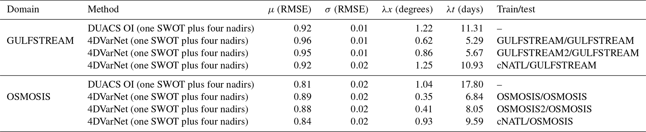
Regarding the BOOST-SWOT OSSE data challenge on the GULFSTREAM domain, we provide both performance with four nadirs and one SWOT plus four nadirs in Table 2. For both settings, the improvement is quite significant with respect to all benchmarked schemes, i.e., not only compared to DUACS OI (Taburet et al., 2019) but also with respect to the recently proposed SSH interpolation schemes Le Guillou et al. (2020), DYMOST (dynamic OI accounting for the SSH nonlinear temporal propagation; see, e.g., Ballarotta et al., 2020) and MIOST (multiscale OI) in Ardhuin et al. (2020). While DUACS OI has a minimal spatial and temporal resolution of 1.42^∘ (four nadirs)$/$1.22^∘ (one SWOT plus four nadirs) and 12 d (four nadirs)$/$11.15 d (one SWOT plus four nadirs), 4DVarNet-SSH reaches 0.83^∘ (four nadirs)$/$0.62^∘ (one SWOT plus four nadirs) and 8.01 d (four nadirs)$/$5.29 d (one SWOT plus four nadirs). It amounts to a gain of up to 33 % in the four-nadir setup and 50 % in the one SWOT plus four nadir configuration.

Figure 6 displays the SSH gradient field of DUACS OI and 4DVarNet-SSH interpolations on 25 October. The comparison to the associated ground truth displayed in Fig. 4b clearly reveals the improvement brought by 4DVarNet-SSH, in particular along the main meander of the GULFSTREAM.

We can draw similar conclusions from the experiments reported in Table 3 and Fig. 7 for the OSMOSIS domain. We may emphasize that 4DVarNet-SSH interpolation for the one SWOT plus four nadir configuration (see, e.g., Fig. 7) retrieves most of the fine-scale features of the SSH fields, which are smoothed out by the optimal interpolation.

5.2 Impact of SWOT data on the interpolation performance

Thanks to its ability to reconstruct finer-scale patterns, 4DVarNet-SSH complements the assessment of the potential impact of SWOT data onto the reconstruction of mesoscale sea surface dynamics. Though the interpolation performance (Tables 2 and 3) improves with the use of SWOT data for all the interpolation methods, the relative improvement strongly depends on the interpolation method. Interestingly, contrary to the DUACS OI scheme, we report a significant improvement when using SWOT data with 4DVarNet-SSH for both GULFSTREAM and OSMOSIS regions. These results emphasize the ability of our scheme to exploit irregularly sampled high-resolution data. For instance, for the OSMOSIS region, we truly benefit from SWOT data for reconstructing mesoscale dynamics up to 0.4^∘ and 7 d, whereas OI DUACS smooths out the altimetry signals in the mesoscale range below 1^∘ and 14 d.

While we report relative gains of 20 %–25 % for the GULFSTREAM region for the different evaluation metrics, it reaches 40 %–60 % for the OSMOSIS domain. We interpret these results as a direct consequence of differences in the space–time sampling of SWOT data for these two regions. As revealed by Figs. 8b and 9b, no SWOT data may be available over 4 (respectively, 1) consecutive days for the GULFSTREAM (respectively, OSMOSIS) domain. This time variability in the sampling pattern translates to a periodic variability in the MSE (mean squared error) time series in the GULFSTREAM region. By contrast, the OSMOSIS region leads to a much lower time variability in the interpolation performance. The PSD-based analysis reported in Figs. 8c and 9c further supports these conclusions.

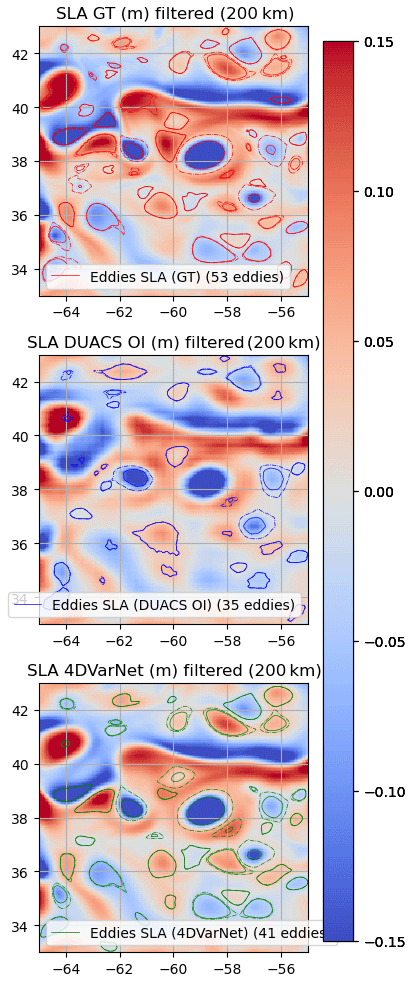
Figure 10 Eddies detected on the GULFSTREAM domain (25 October 2012) over SSH (one SWOT plus four nadirs).

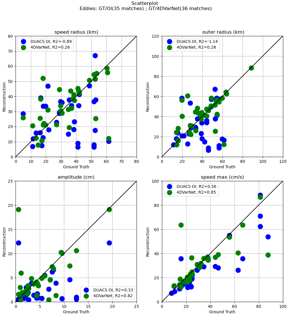
Figure 11 Speed radius (km), outer radius (km), amplitude (cm), and speed max (cm s⁻¹) scatterplots of 4DVarNet/DUACS OI (one SWOT plus four nadirs) vs. ground truth in the GULFSTREAM domain (25 October 2012) for matching eddies.

To complement with the analysis of the contribution of SWOT altimetry on the interpolation performance, Fig. 10 displays the eddy identification results for 25 October 2022 after application of a 200 km high-pass filter when using a one SWOT plus four nadir configuration. Additional figures are given in Appendix B for illustrations of both the GULFSTREAM and OSMOSIS domains in the two observational configurations (four nadirs and one SWOT plus four nadirs). Clearly, 4DVarNet-SSH improves the matching between the true and interpolated eddies (39 vs. 35), and the features of the matching eddies are also more similar to those of the true eddies, in terms of the speed radius (km), outer radius (km), amplitude (cm), and speed max (cm s⁻¹), with respect to their true values. Again, the interpolation of eddy-related dynamics significantly improves with the exploitation of SWOT data.

5.3 Generalization performance

Whereas the results reported in the previous sections involve 4DVarNet-SSH models evaluated on the same domain as the training one, we assess how 4DVarNet-SSH schemes trained for a specific domain may also apply to another one. Besides the GULFSTREAM and OSMOSIS regions, we consider the following three additional domains:

• cNATL domain, which is a larger 20${}^{\circ }\times$40^∘ North Atlantic domain that involves a variety of dynamical regimes,

• GULFSTREAM2 domain, which is a domain similar to the reference GULFSTREAM domain in terms of upper-ocean dynamics but with a disjointed spatial extent, and

• OSMOSIS2 domain, which is a domain similar to the reference OSMOSIS domain in terms of upper-ocean dynamics but with a disjointed spatial extent.

For the one SWOT plus four nadir configuration, we train 4DVarNet-SSH schemes on these three domains. We then evaluate how these models compare with the models reported in Sect. 5.1 for the GULFSTREAM and OSMOSIS domains. We also evaluate how the different models apply to the cNATL domain. Table 4 summarizes the resulting performance metrics.

As expected for each evaluation domain, we retrieve the best performance for the model trained on this domain. For the GULFSTREAM regions, the difference in terms of the minimal temporal scales is negligible, while the minimal spatial scales may exhibit an increase of 30 % when using the model trained on the GULFSTREAM2 domain. This does not hold in the opposite direction when applying on the GULFSTREAM2 domain a model learned on GULFSTREAM, as similar spatial scales resolved in the end. The same conclusions hold for the OSMOSIS regions, except that the minimal resolved temporal scales also display a slight increase (lower than 20 %) over OSMOSIS. These results are consistent with the dynamical properties given in Sect. 4 and support the generalization capabilities of 4DVarNet-SSH schemes. The comparison with the performance metrics reported for the model trained on the cNATL domain suggests that the considered 4DVarNet-SSH parameterization applies to a regional scale. This training configuration only leads to a relatively marginal gain with regard to OI DUACS when applied to the GULFSTREAM region. We report a slightly better performance for the OSMOSIS domain. We expect future work to explore new 4DVarNet-SSH parameterizations, which could better account for basin-scale variabilities.

Table 4 4DVarNet performance on the GULFSTREAM and OSMOSIS domain compared to DUACS OI over the period from 22 October to 2 December 2012 (42 d).

5.4 Uncertainty quantification for 4DVarNet-SSH interpolations

Besides gap-free fields, operational interpolation products generally require us to provide some evaluation of the reconstruction uncertainty. While this is a built-in feature of OI and statistical DA methods, uncertainty quantification may involve specific methodological or computational methods for other data assimilation schemes, among which ensemble methods represent a widely considered family of approaches (see, e.g., Asch et al., 2016). Their common feature is to generate an ensemble of solutions, generally through some randomization process.

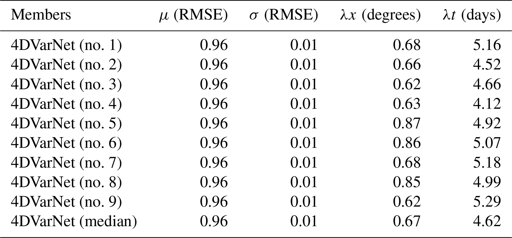
Table 5 4DVarNet performance on the GULFSTREAM domain based on nine different training sessions with a random initialization of both Φ and Γ weights but similar training parameters (number of epochs, learning rates, optimizers, gradient steps, etc.) over the period from 22 October to 2 December 2012 (42 d).

Here, we benefit from the stochastic nature of the training procedure of 4DVarNet-SSH schemes (Goodfellow et al., 2016). Similar to most deep learning schemes, we exploit a stochastic gradient descent during the learning stage and a random initialization of model parameters. As such, for a given training configuration, we can train an ensemble of 4DVarNet-SSH schemes by running multiple training procedures.

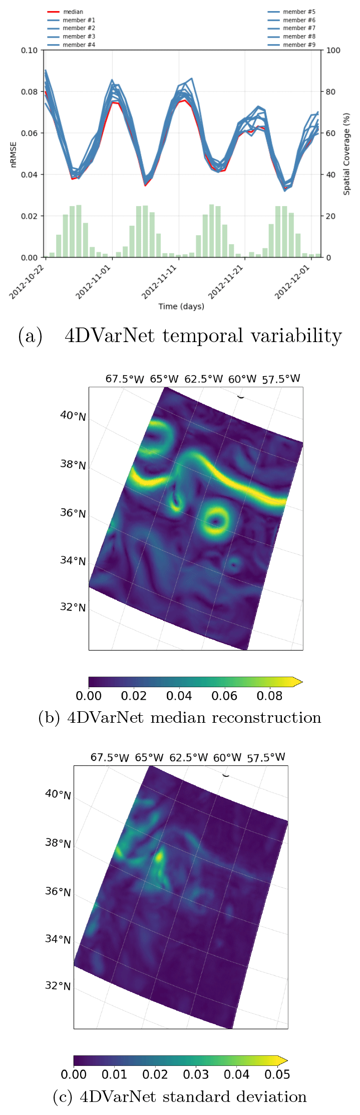
Figure 12 Interpolation performance of an ensemble of nine 4DVarNet-SSH models trained using similar training parameters (number of epochs, learning rates, optimizers, gradient steps, etc.) but different random initialization of both Φ and Γ weights. (a) Spatial RMSE time series on the BOOST-SWOT DC evaluation period, (b) 4DVarNet median run (25 October 2012; GULFSTREAM domain), and (c) its spatial standard deviation.

We apply this approach to build an ensemble of nine 4DVarNet-SSH schemes for a given training configuration, which comprises a training dataset, the considered 4DVarNet-SSH parameterization, and given training hyperparameters (i.e., number of epochs, learning rates, and optimizers). For a given observation time window, we then retrieve nine interpolations from which we can compute a median field and the associated standard deviation. We report the performance metrics for the GULFSTREAM domain of the nine trained models and the median model in Table 5. It reveals the internal variability in the training process. Though it does not reach the best performance, the median model combines a resolved spatial scale below 0.7^∘ and a resolved timescale below 5 d, which is only the case for 6 out of 9 of the trained models. Figure 12a further illustrates this aspect. Interestingly, the standard deviation of the ensemble of 4DVarNet-SSH schemes correlates to the interpolation error, with an R² coefficient of determination equal to 0.86. Even if the scales between the interpolation error and the training-related 4DVarNet internal variability differ (see Fig. 13), the latter can be regarded as an indicator of the interpolation error, usually with an appropriate localization of large errors. In future works, we plan to draw from traditional ensemble DA methods or ensemble Gaussian-based simulations to address all the components of the interpolation error related to the data assimilation scheme.

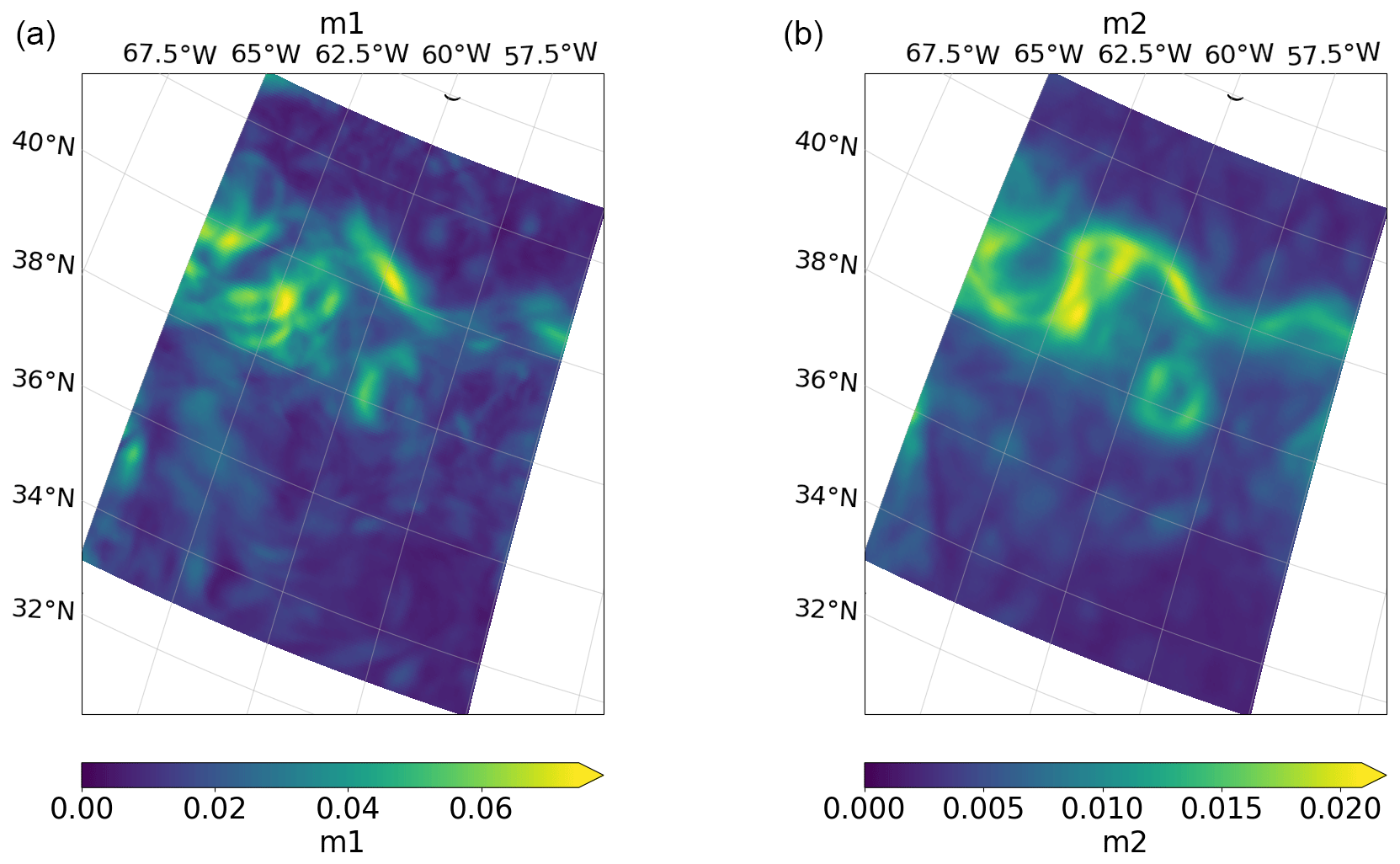
Figure 13 Standard deviation of the 4DVarNet-SSH median ensemble interpolation error (a) and average of the daily standard deviation interpolation errors in the test period (b).

6 Conclusion and discussion

This paper introduced the 4DVarNet-SSH scheme, an end-to-end neural architecture for the space–time interpolation of SSH fields from nadir and wide-swath satellite altimetry data. The 4DVarNet-SSH scheme draws from recent methodological development to bridge data assimilation and deep learning with a view to training 4D-Var DA models and solvers from data. Numerical experiments within an OSSE setting support the relevance of the 4DVarNet-SSH scheme with respect to the state of the art.

We further discuss our main contributions according to three aspects, namely the added value of a deep learning scheme for satellite altimetry and operational oceanography, the exploitation of upcoming SWOT data, and the ability to scale up learning approaches from regional case studies to the global scale.

• Deep learning for satellite altimetry and operational oceanography. This study contributes to a growing research effort regarding the potential benefit of deep learning schemes for space and operational oceanography challenges (see, e.g., Ballarotta et al., 2020). Given the sampling of available satellite and in situ data sources, interpolation problems naturally arise as critical challenges. This study brings additional evidence of the potential of deep learning schemes to outperform the state-of-the-art operational techniques, which are generally based on optimal interpolation and data assimilation. Importantly, we do not rely on the off-the-shelf application of some reference deep learning architectures. The considered class of neural architecture relates to a variational DA formulation, such that it can be regarded as the implementation of a neural and trainable version of a DA model and solver. Our results for satellite altimetry are in line with other recent studies for other ocean parameters, such as sea surface temperature (Barth et al., 2019), suspended sediments (Vient et al., 2022), and 3D temperature and salinity fields (Pauthenet et al., 2022). All these studies support the potential of neural approaches to retrieve finer-scale variabilities from available satellite and/or in situ observations. Regarding satellite altimetry, a future challenge includes the application to real altimetry datasets (see, e.g., the 2021 Observing System Experiments (OSEs) BOOST-SWOT data challenge at https://github.com/ocean-data-challenges/2021a_SSH_mapping_OSE, last access: 2022) and the exploitation of multimodal synergies (Fablet and Chapron, 2022).

• Making the most of SWOT data. Our study brings new evidence that the wide-swath space–time sampling of the upcoming SWOT mission could lead to a very significant improvement in the reconstruction of mesoscale sea surface dynamics. For the considered case study regions, with contrasting dynamical regimes at play and different revisit times of SWOT orbits, we report relative gains from 20 % to 60 % compared to nadir altimetry data only in terms of RMSE and resolved space–timescales. These results assume an error-free SWOT product. Therefore, exploring further how these results could generalize to error-prone (Esteban-Fernandez, 2014; Gaultier and Ubelmann, 2010) and uncalibrated SWOT data (Febvre et al., 2022) is a critical challenge. Preliminary preprocessing of the pseudo-SWOT observations (Metref et al., 2020) to filter out the correlated components and avoid major issues in the assimilation and/or learning process of the interpolation methods may also be considered. The extension of the considered OSSE to multi-SWOT configurations could also provide new means to optimize the deployment of multi-satellite configurations in coming years.

• Scaling up to a global scale with a learning-based scheme. Our numerical experiments focused mainly on a regional scale, typically $\mathrm{10}{}^{\circ }\times \mathrm{10}{}^{\circ }$ domains, as illustrated by the GULFSTREAM and OSMOSIS regions. The reported results support the relevance of the proposed 4DVarNet-SSH parameterization to account for such regional space–time variabilities. Scaling up to a basin scale or even the global scale naturally arises as a key challenge for future work. Through the built-in features of the PyTorch framework and its associated packages, our open-source code can leverage multi-GPU distribution learning schemes and on-the-fly mini-batch generation tools to deal with larger-scale datasets from a computational point of view. To account for a greater diversity in the dynamical regimes at play on the global scale, or even on a basin scale, it also seems necessary to explore more complex 4DVarNet-SSH parameterizations, especially regarding dynamical prior Φ. This could benefit from the variety of neural architectures recently introduced in computational imaging (Barbastathis et al., 2019), especially when using attention mechanisms (Vaswani et al., 2017) to achieve some decomposition of the underlying space–time variabilities.

Appendix A: Fixed-point formulation of the solver

Let note that when replacing both CNN (convolutional neural networks) and/or LSTM cells by the identity operator and the minimization function ${\mathcal{J}}_{\mathrm{\Phi }}(\mathit{x},\mathit{y},\mathrm{\Omega })$ by its single regularization term ${\mathcal{J}}_{\mathrm{\Phi }}^b\left(\mathit{x}\right)$, the gradient-based solver simply leads to a parameter-free fixed-point version of the algorithm, the same used in Beauchamp et al. (2020); Fablet et al. (2019), which is similar to the DINEOF approach (see Fig. A1).

$$\begin{array}{}\text{(A1)}& \left\{\begin{array}{ll}{\mathit{x}}^{(k+\mathrm{1})}& =\mathit{\psi }\left({\mathit{x}}^{\left(k\right)}\right)\\ {\mathit{x}}^{(k+\mathrm{1})}\left(\mathrm{\Omega }\right)& =\mathit{y}\left(\mathrm{\Omega }\right)\\ {\mathit{x}}^{(k+\mathrm{1})}\left(\stackrel{\mathrm{‾}}{\mathrm{\Omega }}\right)& ={\mathit{x}}^{(k+\mathrm{1})}\left(\stackrel{\mathrm{‾}}{\mathrm{\Omega }}\right)\end{array}\right.\end{array}$$

This fixed-point solver is parameter free and easily implemented as a neural network (NN) in a joint solution with the NN parameterization of 𝒥_Φ for the interpolation problem.

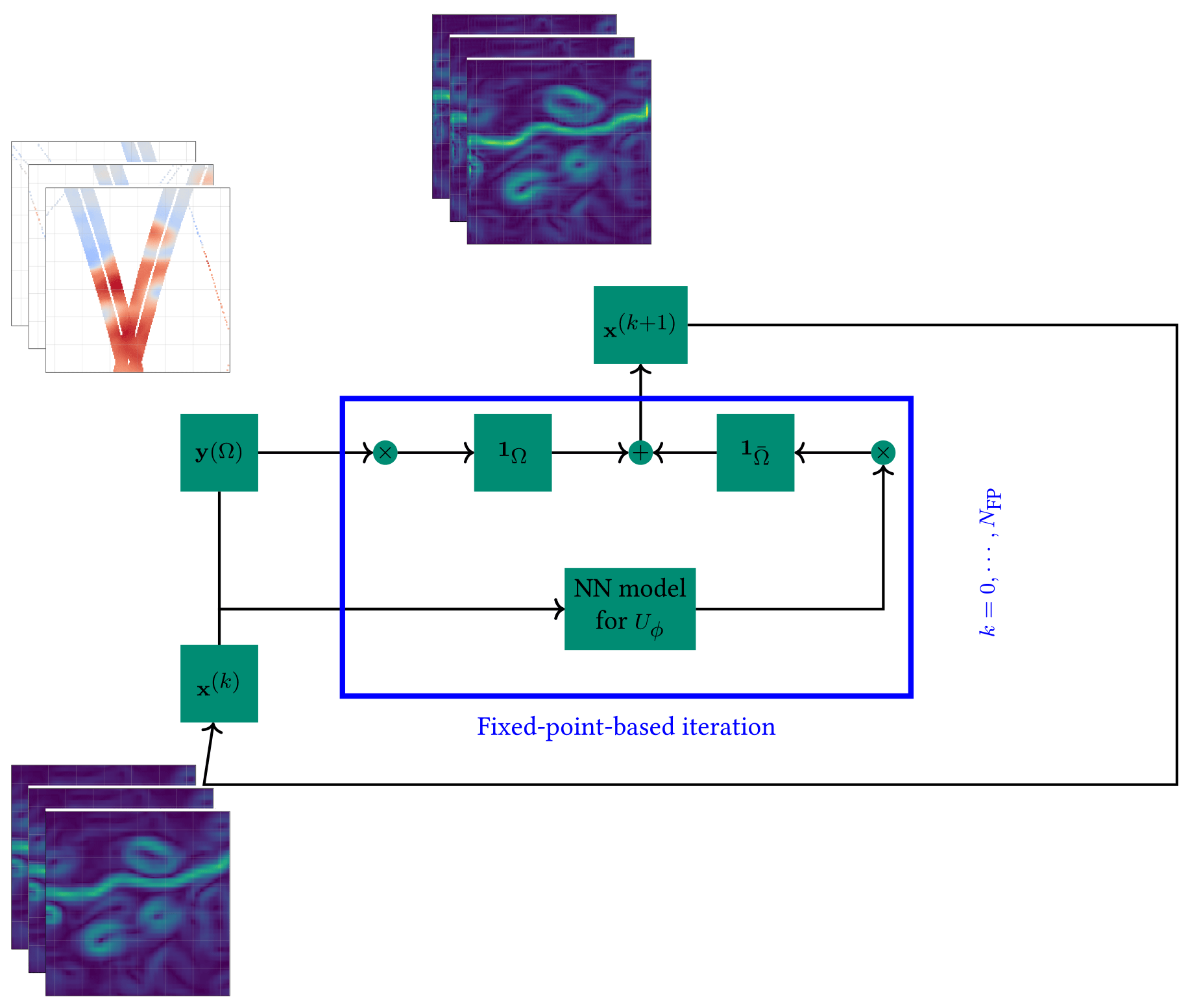
Figure A1 Sketch of the iterative fixed-point algorithm. The upper-left stack of images corresponds to an example of SSH observations temporal sequence, with missing data used as input. The upper-right stack of images is an example of an intermediate reconstruction of the SSH gradient at iteration i, while the bottom-left stack of images identifies the updated reconstruction fields used as new inputs after each iteration of the algorithm.

Appendix B: Additional results on the 4DVarNet generalization capabilities

Table B1 4DVarNet performance on the GULFSTREAM2 and OSMOSIS2 domain compared to DUACS OI over the period from 22 October to 2 December 2012 (42 d).

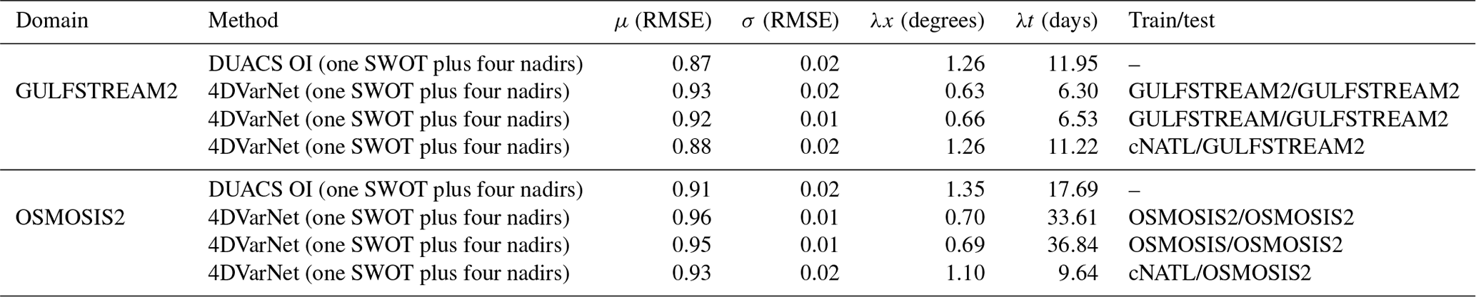
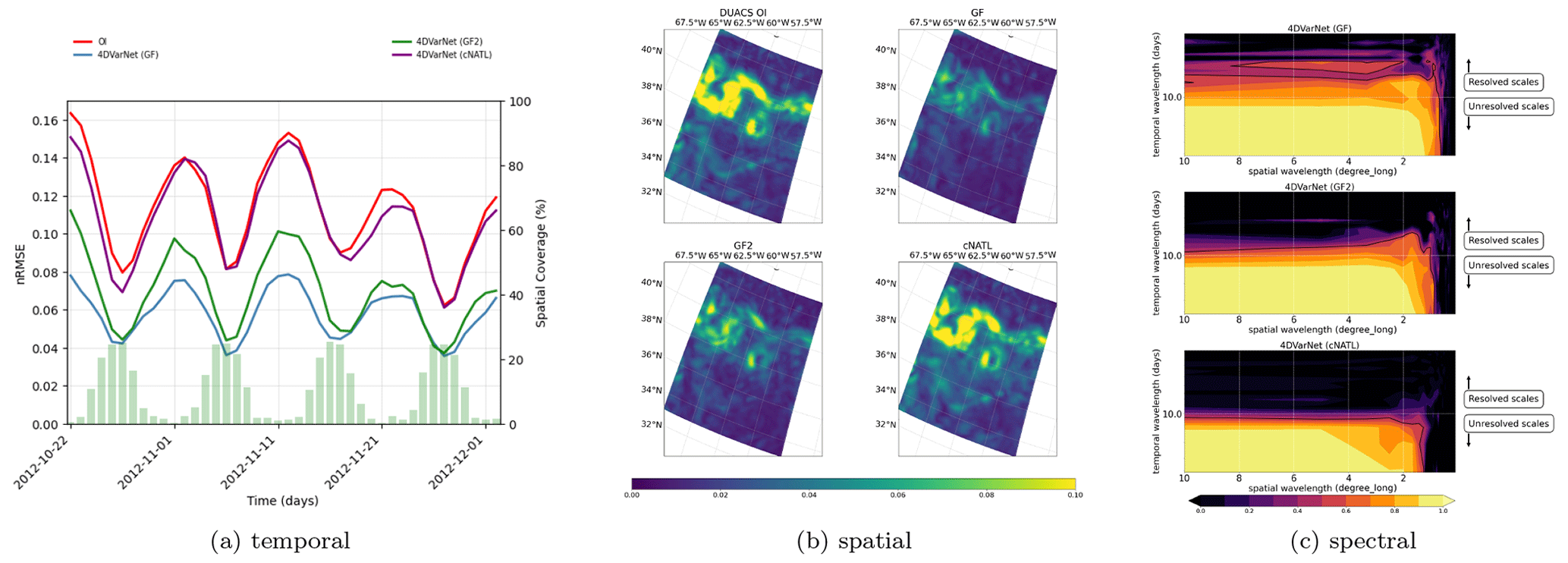
Figure B1 4DVarNet generalization capabilities (GULFSTREAM), with the spatial, temporal, and spectral performance in the BOOST-SWOT DC evaluation period, based on the three different training domains of GULFSTREAM, GULFSTREAM2, and cNATL.

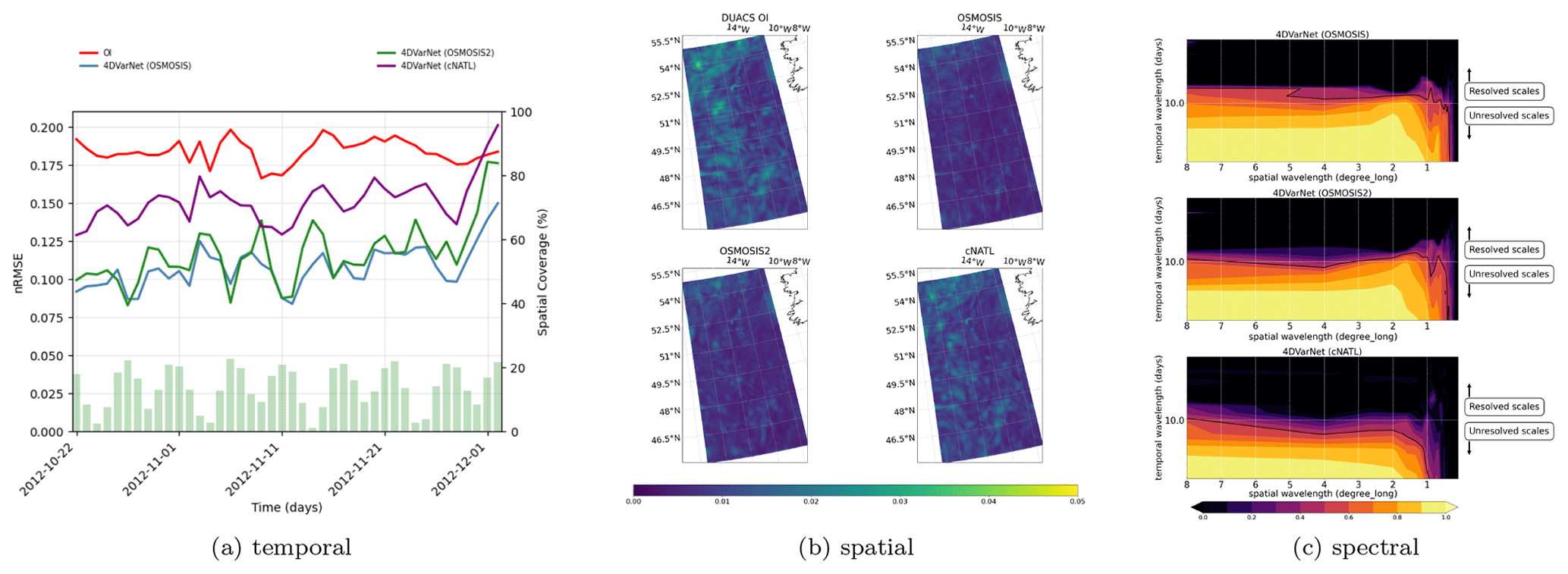
Figure B2 4DVarNet generalization capabilities (OSMOSIS), with the spatial, temporal, and spectral performance on the BOOST-SWOT DC evaluation period, based on the three different training domains of OSMOSIS, OSMOSIS2, and cNATL.

Figure B3 4DVarNet generalization capabilities (cNATL), with the spatial, temporal, and spectral performance on the BOOST-SWOT DC evaluation period, based on the three different training domains of cNATL, GULFSTREAM, and OSMOSIS.

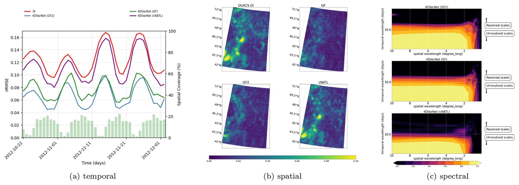
Figure B4 4DVarNet generalization capabilities (GULFSTREAM2), with the spatial, temporal, and spectral performance on the BOOST-SWOT DC evaluation period, based on the three different training domains of GULFSTREAM2, GULFSTREAM, and cNATL.

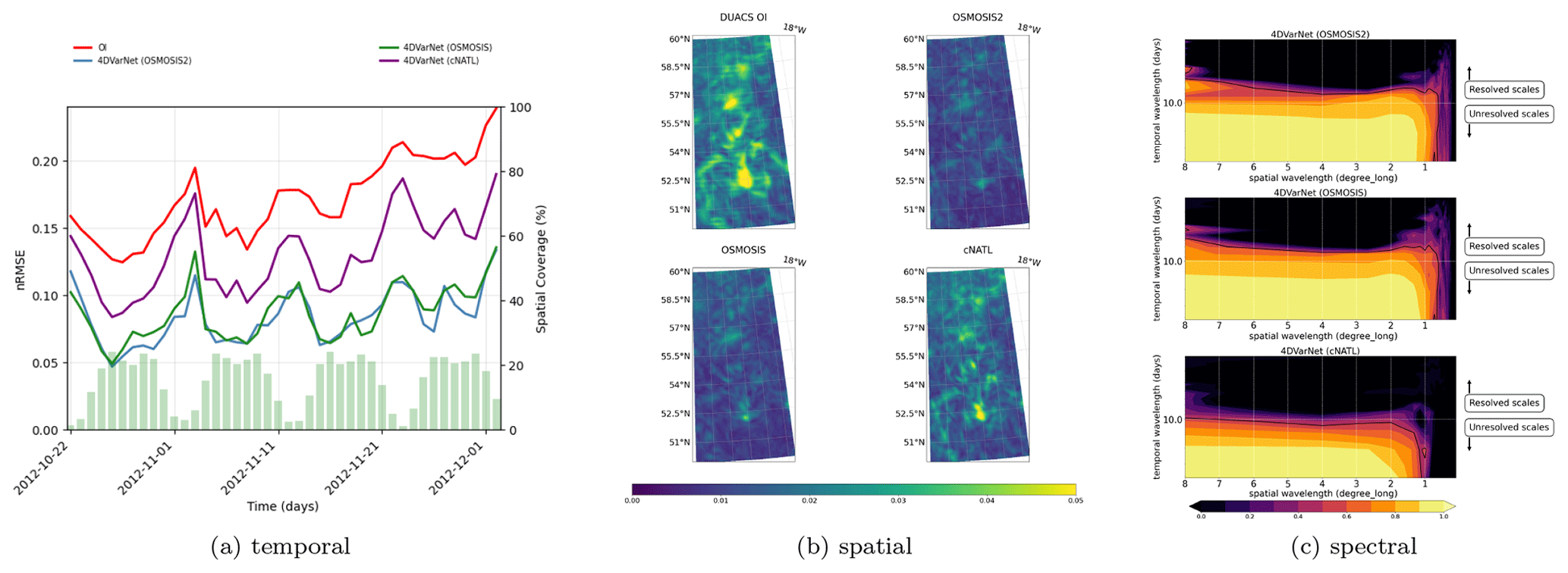
Figure B5 4DVarNet generalization capabilities (OSMOSIS2), with the spatial, temporal, and spectral performance on the BOOST-SWOT DC evaluation period, based on the three different training domains of OSMOSIS2, OSMOSIS, and cNATL.

Appendix C: Eddy identifications

Figure C1 Eddies detected on the GULFSTREAM domain (25 October 2012) over SSH (four nadirs).

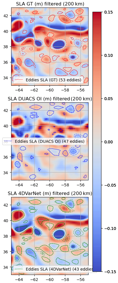
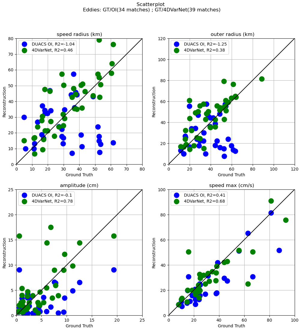
Figure C2 Speed radius (km), outer radius (km), amplitude (cm), and speed max (cm s⁻¹) scatterplots of 4DVarNet/DUACS OI (four nadirs) vs. ground truth on the GULFSTREAM domain (25 October 2012) for matching eddies.

Figure C3 Eddies detected on the OSMOSIS domain (25 October 2012) over SSH (four nadirs).

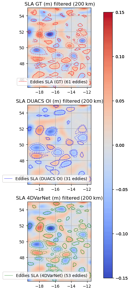
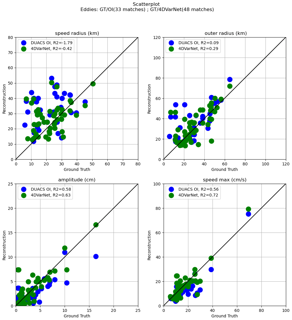
Figure C4 Speed radius (km), outer radius (km), amplitude (cm), and speed max (cm s⁻¹) scatterplots of 4DVarNet/DUACS OI (four nadirs) vs. ground truth on the OSMOSIS domain (25 October 2012) for matching eddies.

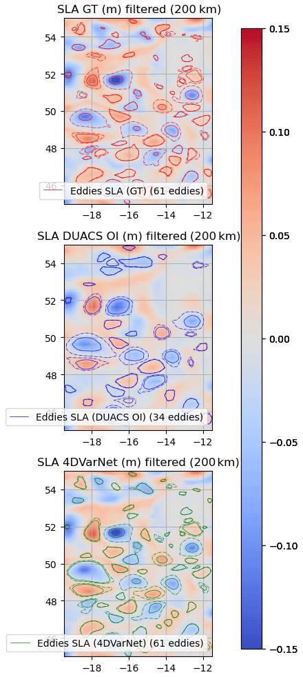
Figure C5 Eddies detected on the OSMOSIS domain (25 October 2012) over SSH (one SWOT plus four nadirs).

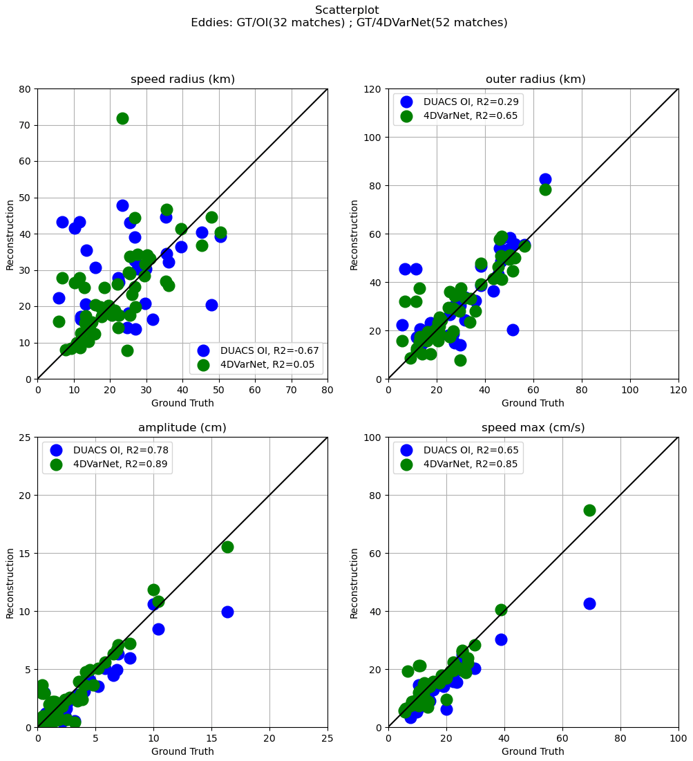
Figure C6 Speed radius (km), outer radius (km), amplitude (cm), and speed max (cm s⁻¹) scatterplots of 4DVarNet/DUACS OI (one SWOT plus four nadirs) vs. ground truth on the OSMOSIS domain (25 October 2012) for matching eddies.