Moana Ocean Hindcast – a  > 25-year simulation for New Zealand waters using the Regional Ocean Modeling System (ROMS) v3.9 model

Here we present the first open-access long-term 3D hydrodynamic ocean hindcast for the New Zealand ocean estate. The 28-year 5 km×5 km resolution free-running ocean model configuration was developed under the umbrella of the Moana Project, using the Regional Ocean Modeling System (ROMS) version 3.9. It includes an improved bathymetry, spectral tidal forcing at the boundaries and inverse-barometer effect usually absent from global simulations. The continuous integration provides a framework to improve our understanding of the ocean dynamics and connectivity, as well as identify long-term trends and drivers for particular processes. The simulation was compared to a series of satellite and in situ observations, including sea surface temperature (SST), sea surface height (SSH), coastal water level and temperature stations, moored temperature time series, and temperature and salinity profiles from the CORA5.2 (Coriolis Ocean database for ReAnalysis) dataset – including Argo floats, XBTs (expendable bathythermographs) and CTD (conductivity–temperature–depth) stations. These comparisons show the model simulation is consistent and represents important ocean processes at different temporal and spatial scales, from local to regional and from a few hours to years including extreme events. The root mean square errors are 0.11 m for SSH, 0.23 ^∘C for SST, and <1 ^∘C and 0.15 g kg⁻¹ for temperature and salinity profiles. Coastal tides are simulated well, and both high skill and correlation are found between modelled and observed sub-tidal sea level and water temperature stations. Moreover, cross-sections of the main currents around New Zealand show the simulation is consistent with transport, velocity structure and variability reported in the available literature. This first multi-decadal, high-resolution, open-access hydrodynamic model represents a significant step forward for ocean sciences in the New Zealand region.

1 Introduction

Interest in the marine realm around New Zealand heavily centres on understanding the drivers of variability from event to decadal timescales in coastal areas. For ocean temperature, this is due to the sensitivity of valuable marine ecosystems to water temperature. While the New Zealand fishing and aquaculture industries are expanding, there is increasing evidence that global Western Boundary Current regions, including New Zealand, are rapidly warming (e.g. Shears and Bowen, 2017). There has been a push in recent years with aquaculture infrastructure moving offshore to minimize the impact of increasing coastal temperatures. For sea level, there is increasing interest in understanding and predicting elevation trends and how these interact with storm surge events and affect coastal infrastructure (e.g. Paulik et al., 2021). For ocean circulation, several efforts are underway to understand pollutant dispersal (e.g. Vennel et al., 2021) and biological connectivity that impact water quality, species distribution, fishing and aquaculture activities (e.g. Chaput et al., 2022; Silva et al., 2019). Although ocean observations provide an essential record of oceanic variability, they are intrinsically scarce – one simply cannot observe everything, everywhere, all the time. Therefore, a consistent, continuous and realistic long integration of a regional simulation can serve as an important source of information. A freely available, multi-decadal, well-evaluated ocean state model that accurately and seamlessly represents coastal and open-water variability across the entirety of New Zealand can provide many benefits to the nation's maritime industries and research purposes. This includes analysis of long-term trends, extreme events and planning for infrastructure developments, as well as research on the physical drivers of the ocean state.

The background ocean state from a free-running model is a key step towards predictive tools such as an ocean reanalyses that combines model and observations through a data assimilation scheme. A robust hindcast is necessary to avoid biases and represent the relevant physical processes for successful data assimilation. This becomes particularly important when implementing strong-constraint assimilation schemes that assume the background model “perfectly” describes the system dynamics (Howes et al., 2017).

Regional simulations are also often used to provide boundary conditions to local models. Due to the large differences between the spatial resolution needed for coastal and/or local studies (typically ≤1 km) and the global simulations (typically ≈9 km), intermediate or regional domains are necessary to transfer information from the large and mesoscales to the local domain. As emphasized by Moore et al. (2019), surface and lateral boundary conditions can represent a significant source of error for such models. To maximize the benefits provided by regional model results, the simulation must include the main dynamical drivers (e.g. winds, tides, boundary currents), have a high enough spatial and temporal resolution to properly represent the regional processes of interest, and be evaluated against a variety of ocean observations to attest its realism.

Keeping these key concepts in mind, a >25-year hindcast named the Moana Ocean Hindcast (also known as Moana Backbone) (Souza, 2022b) was developed for the region around New Zealand. This simulation was performed under the umbrella of the Moana Project. The objective is to provide datasets and products to improve the understanding and prediction of ocean processes in New Zealand. A general project description is provided at https://www.moanaproject.org (last access: 19 December 2022), and the model results are openly available (details available on the project website). The present simulation represents an upgrade on the publicly available ocean hindcasts, especially for New Zealand. The configuration developed for the hindcast and described in the present work was deployed operationally to provide daily forecasts for a period of 7 d, nested inside the Copernicus global ocean operational simulation.

A series of recent papers provide detailed descriptions of the main physical processes driving the circulation around New Zealand and its connection to the broader Pacific, Southern Ocean and the global ocean circulation. Two publications in particular review the main ocean circulation features around New Zealand: Chiswell et al. (2015) describe the large-scale currents and the “blue water” physical oceanography from the literature and recent satellite observations, hydrographic cruises, surface drifters and profiling floats, and Stevens et al. (2019) focus on the continental shelf waters and review prior studies of ocean transport and mixing. In addition, Sutton and Bowen (2019) describe observed changes in ocean temperature around New Zealand in the last 36 years and identify potential drivers of marine heat wave events. The authors combine historical satellite sea surface temperature (SST) observations with water column temperature profiles to identify a warming trend in the waters north of the Subtropical Front that is highly correlated with air temperatures on inter-annual timescales. The strongest warming occurs in the southernmost limit of the local western boundary current – the East Auckland Current, along the east coast of the North Island south of East Cape. Salinger et al. (2020) go a step further and analyse the drivers of summer marine heatwaves. The authors conclude that the events were caused by either atmospheric fluxes or a combination of atmospheric forcing and ocean advection. More recently, Elzahaby et al. (2021) emphasize the role of advection in driving deep and long-lasting marine heatwaves, highlighting the importance of properly representing the ocean currents for a good representation and predictability of such events. While sea surface temperature from satellites has been available for the last >30 years, a high-resolution integral representation of the subsurface ocean structure can only be provided through a continuous model integration.

Given its dimensions and location in the Southwest Pacific Basin, the New Zealand regional circulation is subjected to significant influence from basin-scale flow patterns introduced through the boundaries. Given their typical horizontal resolution, global reanalyses with data assimilation (DA) are expected to represent such dynamics with a significant degree of skill. However, the complex bathymetry, narrow continental shelf, riverine influence and high mesoscale variability add complexities that are beyond the capability of relatively coarse global reanalysis, even considering comprehensive DA.

The repercussions for the regional dynamics are multiple. The interaction of dynamical processes normally excluded from the global simulations with the bathymetry significantly alters the water column density structure. For example, this leads to a poor representation of the temperatures over the continental shelf due to misrepresentation of coastal upwelling in areas such as the Three Kings Islands and the Bay of Plenty (Baxter, 2022; Stevens et al., 2019). The density structure in the Firth of Thames cannot be represented without the inclusion of the input from the Waihou and Piako rivers, influencing the whole Hauraki Gulf (O'Calaghan and Stevens, 2017). The circulation around the Pegasus and Kaikōura canyons cannot be reproduced without a high-resolution bathymetry, affecting cross-shore transports (Lewis and Barnes, 1999).

Here we document and describe the configuration of the 28-year free-running hydrodynamic model and provide an evaluation of the simulation results so that the open-access model can be used with confidence. The hindcast results and model configuration files are available at the Moana Project website (https://www.moanaproject.org, last access: 19 December 2022). The operational forecast system, data-assimilating reanalysis, and their ability in representing and predicting the ocean behaviour will be described in future publications. Section 2 presents the regional simulation configuration and the datasets used to force and validate the model. Section 3 shows a rigorous model evaluation through comparisons between model results and a wide range of observations. Section 4 aggregates the conclusions on the overall quality and limitations of the Moana Ocean Hindcast model.

2 Methods

2.1 Model setup

In the present study, the Moana Ocean Hindcast regional model is developed using the Regional Ocean Modeling System (ROMS) version 3.9. This is a 3D primitive-equation ocean model using hydrostatic and Boussinesq approximations. A full description of ROMS can be found in Shchepetkin and McWilliams (2005) and McWilliams (2009) and on the ROMS website (https://www.myroms.org, last access: 19 December 2022). ROMS has been particularly popular in the oceanographic community in the last decade. There are several hindcasts and operational systems in place using this model, for regions as diverse as Hawaii (Matthews et al., 2012), the deep Gulf of Mexico (Maslo et al., 2020) and the East Australia Current (Kerry et al., 2016; Kerry and Roughan, 2020).

The Moana Ocean Hindcast regional model domain spans ≈161 to ≈185^∘ E and from ≈52 to ≈31^∘ S, with ≈5 km resolution (Fig. 1) with 467×397 grid cells. The grid limits were chosen to include the majority of the New Zealand exclusive economic zone (EEZ), including the Auckland Islands and Chatham Islands, to place the open boundaries far enough from the three New Zealand main islands and to have both the Tasman Front to the north and the Subtropical Front to the south entering the domain through the western boundary, all the while keeping in mind the computational cost for the provision of high-resolution forecasts in an operational setting.

Figure 1 Moana Ocean Hindcast domain and bathymetry and coastal observation locations of daily water temperature (magenta triangle) and tide gauge sea level measurements (red dots) for use in model–data comparison (Sect. 3.4). Temperature locations are sequentially lettered (A–J) from north to south. Land Information New Zealand (LINZ) tide gauge stations are numbered (1–15) to follow anticlockwise Kelvin wave propagation from the southeast station (Port Chalmers) to the southwest (Puysegur). The grey contours show the positions of the 200 and 2000 m isobaths.

ROMS uses a generalization of the classic terrain-following vertical coordinate system (σ coordinates), defined as s coordinates. Stretching functions are used to improve the resolution near the surface and bottom boundaries. In the present study we use the vertical stretching function proposed by Souza et al. (2015), which provides a thinner and less variable surface layer. This is important for the inclusion of the assimilation of sea surface temperature, a following development step in the Moana Project. The present configuration uses 50 vertical layers, with vertical stretching factors of 6 for the surface (θ_s) and 2 for the bottom (θ_b).

The model bathymetry was obtained from a combination of the General Bathymetric Chart of the Oceans (GEBCO) and local sources such as navigation charts and echo sounder surveys. The smoothing of the bathymetry is commonly used in sigma coordinate models to avoid the generation of spurious pressure gradients (PGE – pressure gradient error) in regions of steep slopes due to the model discretization. An iterative approach was adopted to minimize this smoothing and avoid misrepresenting the real basin geometry and, therefore, the dynamics. The smoothing was only applied to grid points where PGE-associated bottom velocities were above the 1 cm s⁻¹ threshold while preserving the total basin volume. This approach was applied before by Shchepetkin and McWilliams (2005), Souza et al. (2015), and others.

A split third-order upstream horizontal advection scheme (Marchesiello et al., 2009) is used for temperature and salinity to help minimize spurious numerical diapycnal mixing in deep waters, while a fourth-order centred differences scheme is used for the vertical advection. The vertical mixing was resolved using the “generic length scale” (GLS) turbulence model configured as a k-kl – equivalent to Mellor–Yamada 2.5 – as described by Warner et al. (2005). Along-isopycnal horizontal mixing was defined for tracers, with along-sigma levels mixing for momentum.

Atmospheric forcing was provided by the Climate Forecast System Reanalysis (CFSR) provided by the National Center for Atmospheric Research (NCAR) (https://climatedataguide.ucar.edu/climate-data/climate-forecast-system-reanalysis-cfsr, last access: 19 December 2022). This includes 10 m winds, air temperature, relative humidity, precipitation rate, downward short- and long-wave radiation, and sea level pressure. Upward long-wave radiation is calculated internally by ROMS. Although more recent atmospheric reanalyses seem to outperform CFSR in other regions, we still lack a detailed analysis and inter-comparison for New Zealand. However, this product has been extensively used in the past and presents a long time series that opens the possibility of expanding the Moana Ocean Hindcast in the future. The fluxes from 42 rivers around New Zealand are included as climatological values obtained from the https://www.data.govt.nz (last access: 19 December 2022) portal. Following Janekovic and Powell (2012), tides were included at the open boundaries as a separate spectral forcing with harmonics provided by the TPXO (TOPEX/Poseidon Global Inverse Solution tidal model) global tidal solution (Egbert and Erofeeva, 2002).

The configuration is nested inside daily results from the Mercator Ocean Global Reanalysis (GLORYS) 12v1 ocean reanalysis (Lellouche et al., 2021), and this choice is described below. Radiation conditions were used for the tracers (temperature and salinity) in the open boundaries, associated with a nudging zone with timescales decreasing from 1 d⁻¹ at the boundary to 0 at ≈200 km towards the domain interior. The 3D velocities were clamped to the GLORYS fields. The free-surface and barotropic velocities used a combination of implicit Chapman and Flather boundary conditions, respectively. Solano et al. (2020) demonstrated these provide optimal results for the representation of tides in coastal models.

The Moana Ocean Hindcast model was run for 27 years, from January 1993 to December 2020. The first year was considered a spin-up period and discarded from the present analysis. The state variables, sea level and velocity components were saved as hourly instantaneous fields and daily mean values. This provides an unprecedented source of high-resolution information, both spatial and temporal, on the ocean conditions and processes around New Zealand.

2.2 Boundary conditions – Mercator reanalysis – GLORYS

A rigorous evaluation of the performance of four readily available global ocean reanalyses in the New Zealand region was conducted by Souza et al. (2020) who showed that GLORYS 12v1 performed best in the region when assessed against local observations. Although all four of the near-global simulations analysed by Souza et al. (2020) (Bluelink ReANalysis, BRAN; HYbrid Coordinate Ocean Model, HYCOM; GLORYS; and CFSR) presented biases in the coastal region, GLORYS showed a more realistic ocean variability and smaller biases in the water column structure in the offshore regions, making it suitable as boundary conditions.

The GLORYS ocean reanalysis is developed by the Copernicus Marine Environment Monitoring Service (CMEMS). It has $\mathrm{1}/\mathrm{12}{}^{\circ }$ horizontal resolution and 50 vertical levels. The reanalysis is generated using the Nucleus for European Modelling of the Ocean (NEMO) ocean model driven at the surface by the ECMWF ERA-Interim reanalysis. It assimilates along-track altimeter observations (sea level anomaly), satellite SST, sea ice concentration, and in situ temperature and salinity vertical profiles from the Coriolis Ocean database for ReAnalysis (CORA) dataset (Szekely et al., 2019) using a reduced-order Kalman filter scheme. In addition, it uses a 3D-Var (3D variational) scheme for the correction of large-scale biases in temperature and salinity. The reanalysis covers the satellite era from 1993 to 2018. For the years 2019 and 2020 the boundary conditions are provided by nowcasts from the Mercator Ocean operational model. This simulation uses the same model configuration as GLORYS.

More details on GLORYS can be found in Lellouche et al. (2021) and the on product page on the CMEMS website (https://data.marine.copernicus.eu/product/GLOBAL_MULTIYEAR_PHY_001_030/description, last access: 19 December 2022).

2.3 Sea level variability forcing

Tides and the inverse-barometer effect can be determinant factors for the representation of the sea surface height and circulation in coastal regions. These phenomena are usually not included in lower-resolution global simulations that provide the boundary conditions for regional models. At least in part, the poor performance of the global reanalyses in the New Zealand coastal region discussed by Souza et al. (2020) can be explained by the absence of such key processes. To include tides, we obtained tidal constituents from the Oregon State University TOPEX/Poseidon Global Inverse Solution (TPXO) version 7.8.1 (Egbert and Erofeeva, 2002). Following the methodology described by Janekovic and Powell (2012), 11 tidal constituents were introduced to our simulation as spectral forcing at the boundaries to the free-surface and barotropic velocity. The inverse-barometer effect is internally calculated in ROMS using the sea level pressure provided by CFSR.

2.4 Observational datasets for model evaluation

A number of publicly available observational datasets were chosen for model evaluation based on their spatial and temporal coverage and the representation of the regional dynamics. The Moana Ocean Hindcast is validated against the observations and the GLORYS reanalysis to provide a comparison against the real world (obs – observations) and an ocean state estimate used to provide boundary conditions (GLORYS). By doing this we seek to highlight the improvement provided by the higher resolution (including bathymetry) and added physical forcing (tides, inverse barometer, rivers, etc.) in the regional simulation. When interpreting the results however, it is necessary to take into consideration that GLORYS assimilates the observations used for the model evaluation, while the Moana Ocean Hindcast is a free-running simulation. It is then expected that GLORYS will present smaller errors when compared to the assimilated observations associated with the large-scale and mesoscale phenomena.

A selection of satellite-derived products and vertical hydrographic profiles are used to evaluate how the simulation represents the large-scale and mesoscale dynamics, while observations of coastal sea level and long-term temperature show the ability of the model in reproducing the hydrodynamic variability in shallow areas over the shelf.

A general overview of the datasets used for model evaluation is given in Table 1, and a description of each is provided in the next subsections.

Table 1 Observational datasets used for the Moana Ocean Hindcast evaluation.

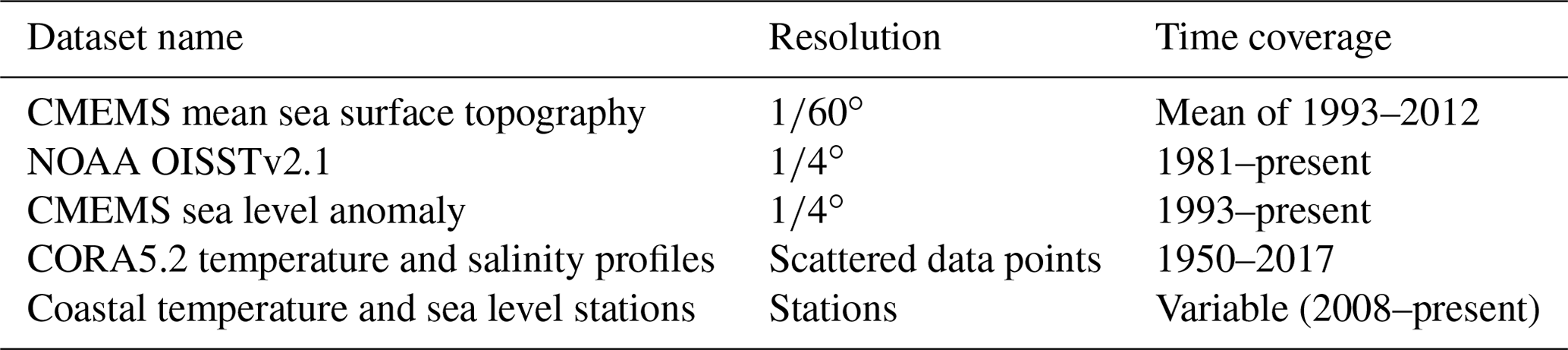
2.4.1 Sea surface height (SSH) – CMEMS products

To evaluate the general pattern of the mean circulation, the simulations were compared to the mean sea surface (MSS) topography and sea level anomaly (SLA) satellite composite products provided by CMEMS (Pujol and Mertz, 2019). The MSS corresponds to a 20-year mean (1993–2012) based on altimetry data, provided at $\mathrm{1}/\mathrm{60}{}^{\circ }$ resolution. The SLA is provided as daily global maps on $\mathrm{1}/\mathrm{4}{}^{\circ }$ resolution. We use the CMEMS “all satellites” product which combines all the available along-track observations at each time to provide the best possible estimate.

2.4.2 Sea surface temperature – NOAA OISSTv2.1

To evaluate the performance of the Moana Ocean Hindcast in reproducing SST we use the Advanced Very High Resolution Radiometer (AVHRR) Optimum Interpolation Sea Surface Temperature (OISST) product provided by NOAA. OISST is an analysis constructed by combining observations from different platforms (satellites, ships, buoys and Argo floats) on a regular global grid. It consists of a $\mathrm{1}/\mathrm{4}{}^{\circ }$ horizontal resolution daily product, which covers the period from late 1981 to the present. More details on the SST product generation are provided by Reynolds et al. (2007).

2.4.3 Temperature and salinity profiles – CORA5.2 dataset

The CORA5.2 dataset described by Szekely et al. (2019) provides a global comprehensive collection of in situ temperature and salinity profiles from 1950 to 2017. It contains data from a diverse set of observational platforms, including mechanical bathythermographs (MBTs) prior to 1965, expendable bathythermographs (XBTs), conductivity–temperature–pressure (CTD) sensors and Argo float profiles from the late 1990s onward. However, most of the observations are limited to 0–2000 m deep – the maximum depth of regular Argo floats. This dataset is used to evaluate the representation of the water column structure in the simulations.

2.4.4 Coastal water temperature and sea level

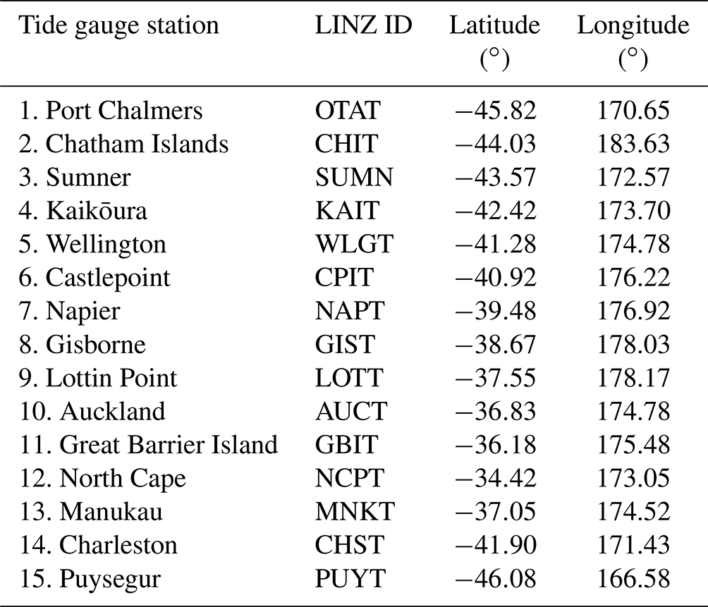
Sea level data are provided through a network of tide gauge stations maintained by Land Information New Zealand (LINZ) (Fig. 1). Sea level data are collected at a 1 min sampling rate and have been available online since 2008 (https://www.linz.govt.nz/sea/tides/sea-level-data/sea-level-data-downloads, last access: 19 December 2022). A total of 15 locations in the tide gauge network are used for model–data evaluation of tidal and sub-tidal sea level variability (Table 2).

Table 2 Land Information New Zealand (LINZ) tide gauge station names, ID and locations for model–data evaluation of sea level.

A total of 10 locations around New Zealand collect daily water temperature measurements from the shore (Table 3). Those from seven stations are collected by the New Zealand's National Institute of Water and Atmospheric Research (NIWA) with digital temperature sensors (Chiswell and Grant, 2019). Additional data are obtained from the University of Otago Portobello Marine Laboratory (daily measurement with handheld mercury thermometer), the University of Auckland Leigh Marine Laboratory and a Datawell Waverider buoy maintained by the Port of Tauranga. Data record continuity and duration vary considerably throughout the hindcast period, with some stations reporting near-complete coverage over the 27-year period (e.g. Evans Bay, Portobello), while other datasets extend ≈4 years (e.g. Bluff). Efforts continue to centrally collate and archive oceanic measurements on the New Zealand Ocean Data Network (NZODN, https://nzodn.nz/portal/, last access: 19 December 2022) and to build co-ordinated ocean observing partnerships across the nation (NZ-OOS – New Zealand ocean observing system;  Callaghan et al., 2019).

Table 3 Coastal daily surface temperature measurement station names, locations and data coverage, where percentage represents the duration of the Moana Ocean Hindcast period. Measurement stations are maintained by NIWA, except where noted.

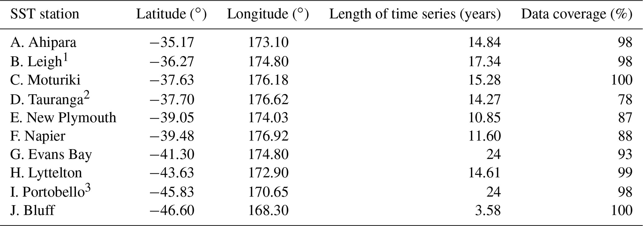
¹ Leigh Marine Laboratory, University of Auckland. ² Tauranga wave buoy, Bay of Plenty Regional Council. ³ Portobello Marine Laboratory, University of Otago.

3 Results and discussion

3.1 Surface

Daily mean fields for SSH and SST were calculated from the Moana Ocean Hindcast to make it comparable to the GLORYS reanalysis and the AVISO (Archiving, Validation and Interpretation of Satellite Oceanographic data) and OISST observational products.

The Moana Ocean Hindcast reproduces well both the large-scale and mesoscale SSH structure (Fig. 2). The Moana Ocean Hindcast temporal mean SSH agrees with the GLORYS reanalysis, which assimilates altimeter observations. It shows the main high (at the northeast of the domain) and low (at the southeast) SSH centres and their respective fronts that reflect the positions of the main large-scale currents at the same locations (Fig. 2). While the high SSH indicates the position of the East Auckland Current (EAUC) and its continuation to the south of the East Cape, the low-SSH front shows the position of the Southland Current and its continuation as the Subtropical Front as it veers eastward and detaches from the coast. Gradients in SSH are generally stronger in the Moana Ocean Hindcast, especially in the region of the EAUC to the north and east of the North Island of New Zealand. This constitutes in sharper fronts and stronger boundary currents, desired in a higher-resolution model as discussed in Sect. 3.3.

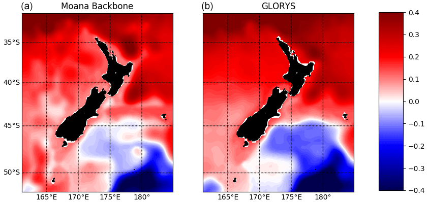
Figure 2 Temporal mean SSH (m) from the free-running Moana Ocean Hindcast (a) and the data-assimilating GLORYS (b) simulations. The general patterns of the SSH are reproduced by both models.

Table 4 Summary of the deviations for the SSH (m) and SST (^∘C) of the Moana Ocean Hindcast simulation compared to the AVISO and the OISST observational gridded products, respectively. Statistics for the RMSE, mean absolute error (MAE) and maximum absolute error (MaxAE) are presented.

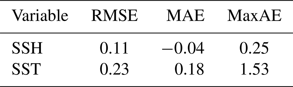
Figure 3 shows a similar pattern for the variance of the SSH between the Moana Ocean Hindcast and GLORYS simulations and the gridded AVISO observational product. The Moana Ocean Hindcast shows larger overall variance, as expected due to its higher horizontal resolution. With the higher resolution comes a better representation of oceanic eddies and fronts and the process that lead to their formation such as instabilities. More energy is transferred between scales, leading to stronger variability, and less is left to be parameterized usually using a diffusion operator. These larger variability values are more evident in the regions corresponding to the eddying EAUC and its continuation to the east in the Subtropical Front and the area influenced by the northern branch of the Antarctic Circumpolar Current in the southeast extremity of the domain. Ballarotta et al. (2019) showed that the effective spatial resolution of the altimetry maps around New Zealand is between 150 and 200 km, marginally resolving the mesoscale eddies.

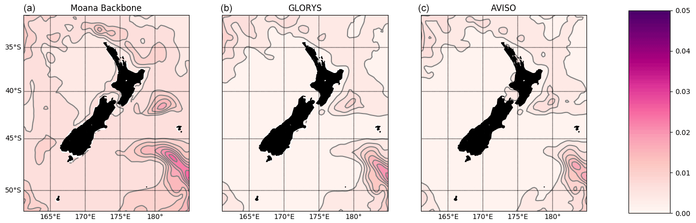
Figure 3 Variance of the SSH (m²) from the free-sunning Moana Ocean Hindcast (a), the data-assimilating GLORYS (b) simulations and the AVISO product (c). Although the same general distribution is observed, the Moana Ocean Hindcast presents stronger variability due to its higher spatial resolution. Contours are provided at 0.01 m² intervals.

To evaluate the spatio-temporal structure of the SSH variability, the elevation fields from the Moana Ocean Hindcast and GLORYS simulations and the AVISO observations were decomposed into the empirical orthogonal functions (EOFs). Following Ballarotta et al. (2019), a 40 d low-pass filter was used on the data prior to the EOF decomposition. The authors show that the mean temporal resolution of the AVISO altimetry maps at the Equator is 34 d, with values ranging between 35 and 42 d around New Zealand. Figure 4 shows the first EOF, which explains 35 %, 38 % and 37 % of the variance for the Moana Ocean Hindcast, GLORYS and AVISO, respectively, and the remaining EOFs have contributions 1 order of magnitude smaller. The overall pattern is similar between the simulations and observations. The Moana Ocean Hindcast shows stronger high-frequency variability, as evidenced in the principal-component time series. This can be related to a series of factors, including the higher horizontal resolution and the inclusion of physical processes such as tides and the inverse-barometer effect. The seasonal to inter-annual variability of the SSH throughout the domain is well reproduced.

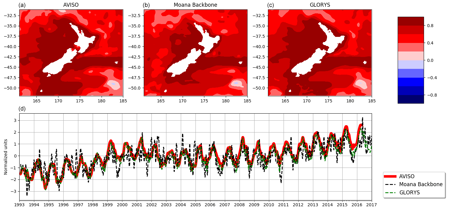
Figure 4 Empirical orthogonal function (a, b, c) and principal component (d) decomposition of the 40 d low-pass filtered SSH from the Moana Ocean Hindcast (a) and GLORYS simulations (b) and the AVISO observational product (c).

The Moana Ocean Hindcast also reproduces the SST throughout the domain well, with a good representation of variability in a range of timescales from sub-seasonal to inter-annual as shown in Fig. 5. It is interesting to observe how the historical high-temperature peak in 2018 is well reproduced in the simulation. Individual high-temperature anomaly events with a duration on the order of a few days, such as marine heatwaves, were also reproduced and will be explored in depth in separate publications.

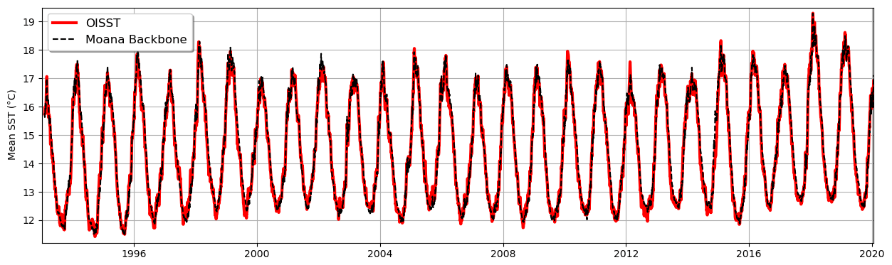
Figure 5 Domain-averaged SST (^∘C) for the Moana Ocean Hindcast and the OISST observational product. The Moana Ocean Hindcast model is able to reproduce the observed SST variability ranging from sub-seasonal to inter-annual.

The root mean square error (RMSE) and bias (BIAS) maps in Fig. 6 show deviations of the model in relation to the OISST observational products. The model errors are concentrated in the coastal waters and the position of strong eddying fronts. The bias pattern is reminiscent of the differences showed by GLORYS in Fig. 6 of Souza et al. (2020), which shows overall negative values in the coastal region and positive values in the east of the domain – especially in the Subtropical Front area. These differences relate to a series of factors: (a) the fact that a free-running simulation is in general not able to place eddies in the exact same place and time of the observations, (b) the relatively coarse resolution of the OISST product that tends to smooth the frontal regions, and (c) issues related to the observation of SST from satellites close to the coast and in a region notorious for its high cloud coverage. While (a) and (b) are intrinsic limitations of the model and the satellite product, respectively, (c) is further explored in Sect. 3.4.2, where we evaluate the Moana Ocean Hindcast results against coastal temperature stations. Indeed, regions of larger RMSE agree in general with areas of large variability as shown in the SSH variance map in Fig. 3. Two notable exceptions are the RMSE hotspots at 43^∘ S, 174^∘ E and 48^∘ S, 166^∘ E. These two regions correspond to fronts of the Southland Current where large SST gradients are present. Therefore, we estimate that the RMSE is related to differences in the location of the front in the simulation in relation to the OISST product. Although this can be due to errors in the model, one should keep in mind that the $\mathrm{1}/\mathrm{4}{}^{\circ }$ Optimum Interpolation Sea Surface Temperature product will have smoothed fronts which will contribute to (if not dominate) the large RMSE.

Figure 6 RMSE and BIAS of the Moana Ocean Hindcast SST (^∘C) in comparison to the OISST observational product. It shows that differences between the simulation results and the OISST are concentrated in the locations of strong fronts and the coast. These relate to the fact that this is a free-running simulation, differences in resolution and the inability of the observational product to represent temperatures close to the shoreline.

The errors for the SSH and SST are summarized in Table 4. The Moana Ocean Hindcast shows a very good agreement with the observational products, especially for a non-assimilating simulation. While the performance for SSH is similar to global simulations when the whole domain is considered, the present results show smaller errors for SST. The errors in the global simulations, including GLORYS, are described by Souza et al. (2020). As presented above, the SSH errors must be taken with care since the Moana Ocean Hindcast simulation includes tides and the inverse-barometer effect that are not included in the GLORYS reanalysis and are removed from the satellite data prior to the generation of the gridded product. Therefore, the differences are at least in part due to the improved physics. This is evaluated in detail when we compare the model results against tide gauge elevations in Sect. 3.4.1.

While the MaxAE is simply the maximum absolute difference between the two datasets, the RMSE and MAE in Table 3 were calculated using the below formulations:

$$\begin{array}{}\text{(1)}& {\displaystyle }\mathrm{RMSE}=\sqrt{{\displaystyle \frac{\mathrm{1}}{n}}{\mathrm{\Sigma }}_{i=\mathrm{1}}^n(\mathrm{obs}-\mathrm{model}{)}^{\mathrm{2}}},\text{(2)}& {\displaystyle }\mathrm{MAE}=\sum _{i=\mathrm{1}}^n|\mathrm{obs}-\mathrm{model}|,\end{array}$$

where n is the number of data points, obs is the observations and model is the simulation results.

3.2 Water column

We compare the daily mean fields from the Moana Ocean Hindcast model results against all the vertical profiles in the CORA5.2 dataset. A total of 118 040 temperature and 54 787 salinity profiles were used in the model evaluation. These are unevenly distributed in time and across the model domain. Therefore, only aggregated information and scatter maps are presented. The model results were co-located in time and linearly interpolated in space to the observations.

The RMSE for both temperature and salinity (Fig. 7) show larger errors near the surface – in particular in the top 20 m. Such an increase is related to the surface fluxes provided by the atmospheric simulation (CFSR) used to force the Moana Ocean Hindcast. The error decreases steadily with depth, with values in general under 1 ^∘C for temperature and 0.15 g kg⁻¹ for salinity below the mixed layer. These compare well with the GLORYS errors presented by Souza et al. (2020).

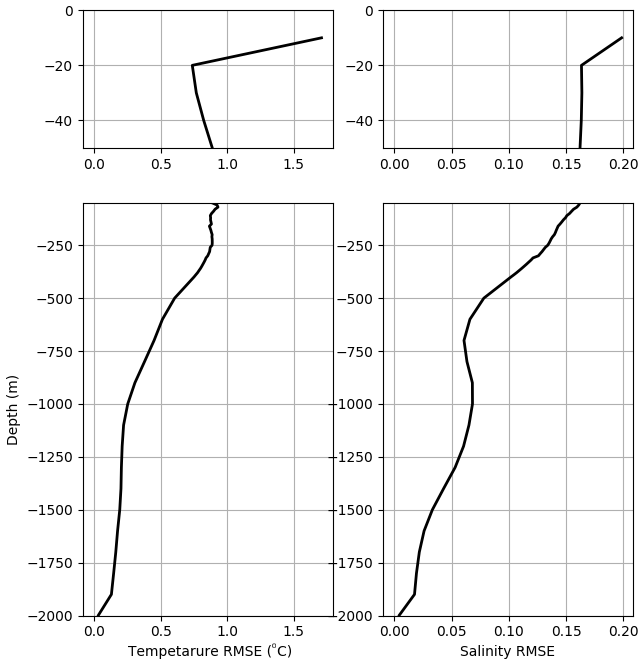
Figure 7 RMSE profiles for temperature (^∘C) and salinity (g kg⁻¹) of the Moana Ocean Hindcast simulation in relation to the CORA5.2 observations. A zoom-in of the first 50 m where the larger differences are observed is provided in the upper row.

Looking at the difference maps in Fig. 8 one can see a general pattern of warmer and saltier waters to the east of New Zealand and the opposite to the west. As shown in the RMSE profile (Fig. 7), the differences are larger closer to the surface. Despite the difficulty in asserting the reasons behind such differences, they seem to be in part related to the surface forcing from CFSR and in part due to the boundary conditions from GLORYS. Souza et al. (2020) show a similar pattern of differences for GLORYS in the thermocline and deep waters.

Indeed, the boundary conditions from GLORYS set the large-scale water mass structure that is fed to the model domain. However, the presence of a water mass formation zone in the Subtropical Front provides a pathway through which atmospheric signals coming from CFSR can penetrate to depths below the thermocline and influence the 3D density structure – especially for central and deep waters.

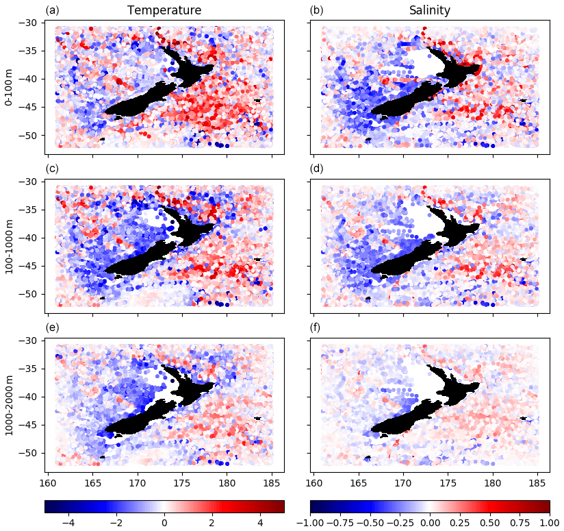
Figure 8 Scatter map of the depth mean deviation (by layers) of the Moana Ocean Hindcast results from the CORA5.2 temperature (^∘C; a, c, e) and salinity (g kg⁻¹; b, d, f) observations. The differences are divided by slabs corresponding roughly to the mixed layer (0–100 m; a, b), thermocline (100–1000 m; c, d) and deep waters (1000–2000 m; e, f). A geographic distribution pattern is evident in the model result differences, which follow the same overall distribution presented by the GLORYS reanalysis.

Modelled and observed surface mixed-layer depths (MLDs) are compared seasonally and spatially over the hindcast period (Fig. 9). Surface MLDs are estimated for individual CORA5.2 temperature profiles and Moana Ocean Hindcast temperature fields interpolated (nearest neighbour in time, linear horizontally and vertically) onto the CORA5.2 profiles, with MLDs detected using a temperature difference criterion of 0.2 ^∘C (de Boyer Montégut et al., 2004) and a MATLAB implementation of the Holte and Talley (2009) MLD algorithm available from http://mixedlayer.ucsd.edu/ (last access: 19 December 2022).

Results from the MLD analysis of the CORA5.2 observations (Fig. 9, first column) are consistent with the literature and the expected seasonal dynamics of MLD thickness (Holte et al., 2017). During austral summer, MLDs across the region 31–45^∘ S are shallow at <25 m, and the variability, indicated by 5th and 95th percentiles, is low (Fig. 9, last column) with both metrics increasing toward higher latitude. Seasonal thickening of the MLD and increased variability in MLDs are evident across the entire domain with maximum MLDs reached during austral winter. The deepest MLDs and highest MLD variability is seen south of 45^∘ S, particularly along the borders of the Campbell Plateau and northern limit of the Antarctic Circumpolar Current, where MLDs exceed 250 m.

The model (Fig. 9, second column) reproduces the seasonal and spatial pattern well in MLDs across New Zealand seen from CORA5.2, although there are some notable differences. These are evident by comparing differences between the model and corresponding observed MLDs over the entire domain (Fig. 9, third column). The model generally underestimates the MLD, with a domain-wide mean difference of 7–12 m, depending on the season. The most notable differences are present in a halo around New Zealand during austral winter and spring, as well as in the vicinity of the Campbell Plateau. A comparison between the 5th and 95th percentiles around the zonal-mean MLDs from the model and observations (Fig. 9, last column) provides a further assessment of the model's performance in capturing temporal variability of the MLD. Generally, the model MLD variability falls within the envelope of the observed MLD variability for all latitudes and season; however, the 95th percentile of model MLDs is consistently lower than found in observations, suggesting that the model is underestimating the depth of the deepest mixed layers in all seasons. We note that the accuracy of the daily MLDs is important for a range of applications, for example when diagnosing drivers of marine heatwaves (Elzahaby et al., 2021).

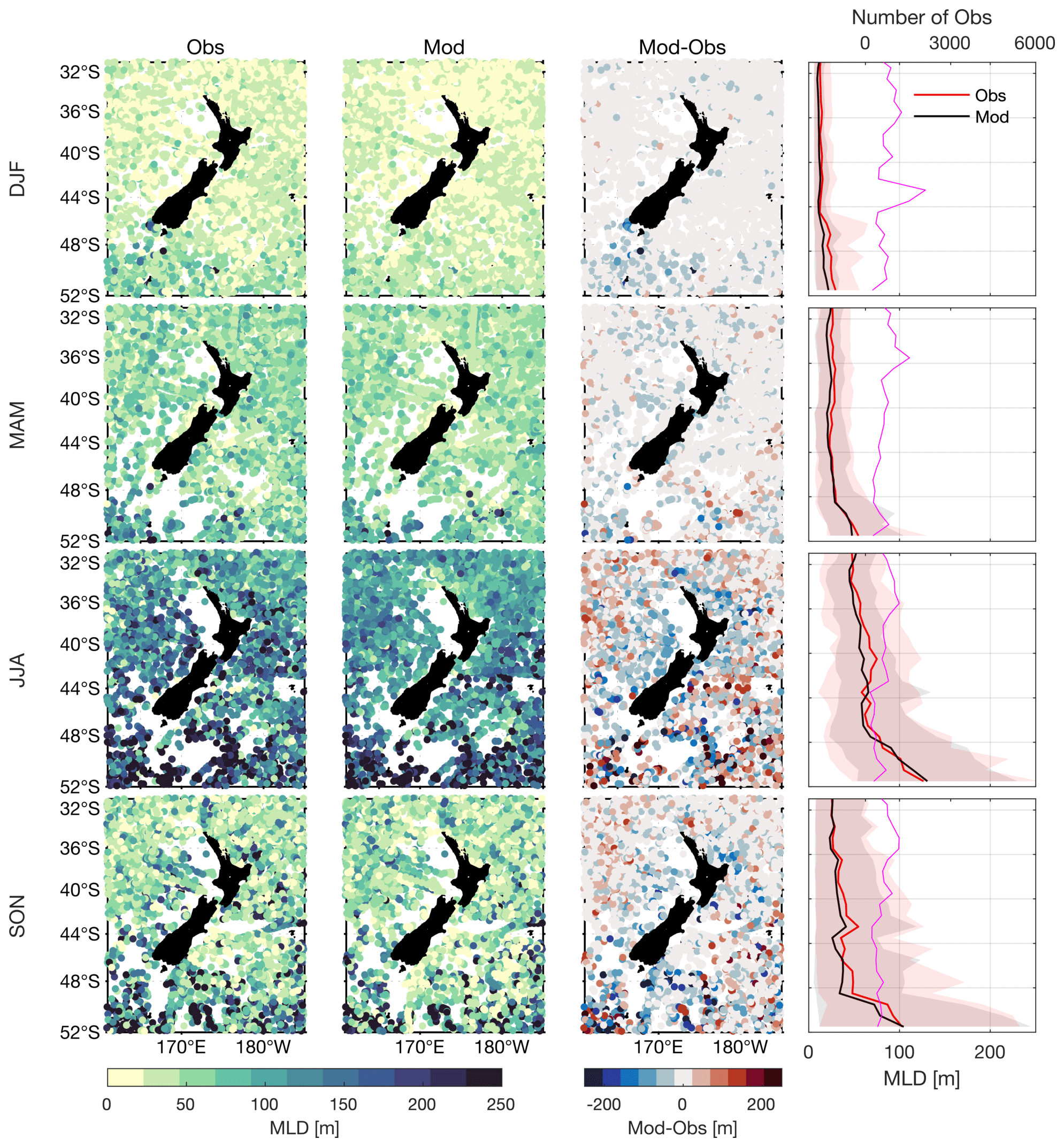
Figure 9 Seasonal mixed-layer depths (MLDs) computed from temperature profiles from CORA5.2 (first column), the Moana Ocean Hindcast (second column) and the difference between these (third column) within the region 31–52^∘ S, 161–185^∘ E over the period 1994–2017 using a temperature threshold method (Holte and Talley, 2009). The last column indicates the zonal-mean MLD from the Moana Ocean Hindcast (black solid) and CORA5.2 (red solid), together with the 5th and 95th percentiles (shaded). Also shown are the number of temperature profiles in each latitude band (magenta solid). DJF: December–January–February, MAM: March–April–May, JJA: June–July–August, SON: September–October–November.

3.3 Boundary current transport

The mean surface currents from the Moana Ocean Hindcast (Fig. 10a) represent New Zealand's major boundary currents as described in Chiswell et al. (2015) and Stevens et al. (2019). Current variability is greatest over the eddy-dominated regions where the EAUC separates from the coast (off North Cape, East Cape and Wairarapa), while the more coherent Southland Current shows little directional variability (Fig. 10b). To quantify New Zealand's major boundary current transport and variability, we choose eight shore normal sections where the flow is maximum (Fig. 10a, sections 1–8) and four sections where major boundary currents turn offshore (Fig. 10a, sections A–D).

The volume transport through each section is computed daily and is given by

$$\begin{array}{}\text{(3)}& \mathrm{Trans}={\displaystyle \frac{\mathrm{1}}{{\mathrm{10}}^{\mathrm{6}}}}\underset{-D}{\overset{\mathrm{0}}{\int }}\underset{x_{\mathrm{0}}}{\overset{x_i}{\int }}\left(\mathit{v}\right)\mathrm{d}x\mathrm{d}z,\end{array}$$

where x₀ to x_i is the cross-section distance, −D is the depth of the section, v is the daily-averaged across-section velocity and the transport has units of Sv (1 Sv =10⁶ m³ s⁻¹). The section length (which corresponds to the distance offshore for sections 1–7, Fig. 10a) and depth over which the transport is computed are defined by the +0.05 or −0.05 m s⁻¹ contour in the velocity mean (the sign depending on the mean flow direction). In cases where the current core is not well defined (i.e. Fiordland Current, Westland Current and western coast of New Zealand), a distance of 200 km offshore is chosen. The transport is computed daily for the 25-year hindcast.

The means and standard deviations of the daily volume transport over the long-term simulation, as well as the distances and depths over which transport is computed, are presented in Table 5. The Cook Strait section in our model is ≈15 km wide (represented by only three grid cells), compared to, in reality, a 22 km wide strait at its narrowest region.

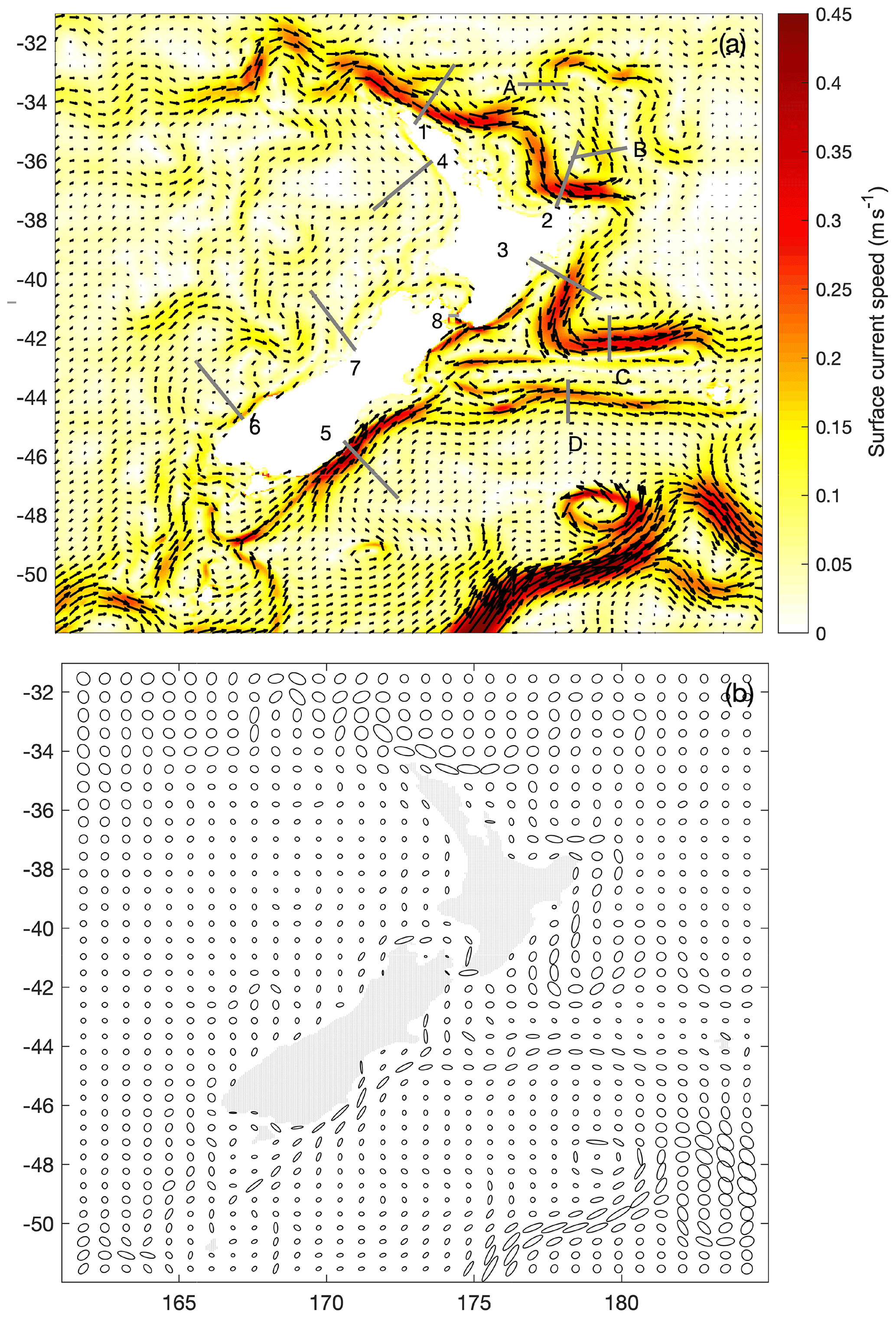
Figure 10 Mean surface current speed and velocity vectors (a) and velocity variance ellipses (b). Data are from the daily-averaged output from the 25-year Moana Ocean Hindcast (also known as Moana Backbone). Sections for the transport calculations are shown.

Table 5 Alongshore transport (Sv) through cross-shore sections (Fig. 10, sections 1–8) and the offshore sections (Fig. 10, sections A–D) computed daily for the 25-year hindcast. The section length (which corresponds to the distance offshore for sections 1–7) and depth over which the transport is computed is defined by the +0.05 or −0.05 m s⁻¹ contour in the velocity mean (the sign depending on the mean flow direction), expect in cases where there is no defined core, in which case a distance of 200 km offshore is chosen. Section length and depth are included in the table. FD: full depth.

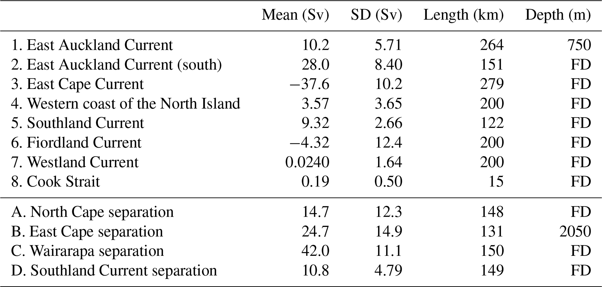
We evaluate the model's ability to reproduce the large-scale circulation through long-term-averaged volume transport comparisons with estimates presented in the literature. We limit this model assessment to three sections, corresponding to the EAUC, ECC (East Cape Current) and SC (Southland Current), given the extensive fieldwork carried out to date along the eastern margin of the New Zealand continental shelf. Volume transport calculations are sensitive to the dataset used (e.g. in situ, altimetry or model) and the section area over which transport is computed, which is directly dependent on data availability and/or assumptions made in the definition of the boundary current spatial extent (e.g. horizontal and vertical). Nevertheless, comparing in situ versus modelled transport estimates allows for a reasonable quantitative assessment of the model's representation of the boundary currents.

Overall, modelled mean volume transport estimates from the main boundary currents are in agreement, within the range of the standard deviation, with values presented in the literature, indicating that the model reproduces the flow structure and magnitude of New Zealand's major boundary currents with a good degree of accuracy. Below is a more detailed description of how each boundary current compares with previous in situ and/or remote-based volume transport estimates.

East Auckland Current

The mean modelled transport estimated for the EAUC, northeast of North Cape (Fig. 10, section 1), is 10.2±5.71 Sv (Table 5). Our mean transport is found to be within the range of those reported in Roemmich and Sutton (1998) (9.0 Sv) and Stanton and Sutton (2003) (9.5±5.5 Sv), derived from XBT climatology and altimetry, respectively. Similar values were also encountered by Fernandez et al. (2018) in the region using a significantly longer dataset. Their results show values of 12.4±4.5 and 12.6±2.6 Sv derived from 21 years of altimetry and 28 years of XBT measurements, respectively, and 8.4±6.2 Sv from CTD casts along same the altimeter track. These values are also consistent with a volume transport of 8–15 Sv derived from Argo float trajectories in the same region (Bowen et al., 2014).

East Cape Current

The mean modelled transport estimated in the ECC region (Fig. 10, section 3) is 37.6±10.2 Sv (Table 5). This estimate is considerably higher than those presented in the literature; however key difference in the calculation methods and locations exist. The ECC transects of Fernandez et al. (2018) are to the north and to the south of our chosen transect and estimate altimeter-derived mean and standard deviation of volume transports of 10.5 Sv (2.7 Sv) and 5.6 Sv (2.2 Sv), respectively. The transect that is further to the north (directly off East Cape) is located where current velocities are considerably lower, while the transect to the south is downstream of the peak current velocity, transverses the equatorward counter current and does not extend offshore into the core of the ECC (Fig. 10).

Furthermore, their calculations purposely excluded transport due to recirculation of eddies. In contrast, our section was chosen where the ECC (south of East Cape) shows the strongest velocities, and transport is considerably strengthened due to recirculation of the Wairarapa eddy. This strengthening due to recirculation is also seen in the East Australian Current (EAC) (Kerry and Roughan, 2020). Previous attempts to estimate transport use satellite altimetry combined with subsurface observations to estimate the vertical structure of the current and assume a level of no motion of 2000 dbar (e.g. Fernandez et al., 2018). In addition, transport estimates are highly sensitive to the distance offshore over which transport is calculated.

A detailed discussion of the differences in calculation methods and the significantly higher ECC transport estimates compared to previous estimates in the literature, including Fernandez et al. (2018), is presented in Kerry et al. (2022). This study is indeed the first study that we are aware of that has estimated transport in the ECC at this latitude, where velocities are strongest. Furthermore our transport estimate encompasses the entire cross-section through the current (based on the 0.05 m s⁻¹ mean velocity contour) extending 279 km offshore and to the full water depth (below 3000 m). Chiswell (2005) estimates the transport in the ECC feeding the Wairarapa eddy to be 15 Sv relative to the 2000 dbar, yet they note that this is likely to be an underestimate as the current core extends deeper than the 2000 dbar (Chiswell, 2003).

Southland Current

The mean modelled transport estimated in the SC region (Fig. 10, section 5) is 9.32±2.66 Sv (Table 5). Similar values (10.4 Sv) have been reported by Chiswell (1996), inferred from geostrophic velocities estimated from a 1-year-long CTD survey conducted along a transect off Oamaru (virtually the same location as for the section adopted here). These values are also in agreement with those found by Sutton (2003) (8.3±2.7 Sv) obtained from full-depth transport estimates derived from CTD surveys carried out between the years 1993 and 2000 over a region offshore Otago Peninsula encompassing the north of Campbell Plateau and south of Chatham Rise. More recently, Fernandez et al. (2018) derived the SC volume transport from 1993–2012 altimeter data across two sections, south and north of our reference section, reporting 7.2±0.8 and 10.6±1.0 Sv, respectively.

Cook Strait

We also assess the mean cross-sectional transports through the Cook Strait (Fig. 10, section 8) given the significance and role that volume exchange across the strait plays in the upper-water-column ocean circulation in the central New Zealand region. The mean modelled transport across the strait is 0.19±0.50 Sv (Table 5). The high standard deviation relative to the mean illustrates the variable nature of the residual transport, and it can be expected that the mean transport is sensitive to the time period over which the mean is taken. Stevens (2014) estimated a mean transport of 0.25 Sv based on residual (low-pass filtered at 48 h) currents from 20-month continuous acoustic Doppler current profiler (ADCP) measurements. Hadfield and Stevens (2021) estimate a 3-year mean volume flux of 0.42 Sv±0.08 Sv based on modelled–measured adjustments. Our modelled value may be lower as the Cook Strait width is 15 km at its narrowest point in the model, compared to the real width of 22 km.

3.4 Coastal sea level and water temperature

3.4.1 Coastal sea level

Observed and modelled sea level variability are compared over a 3-year period (January 2015–December 2017). The modelled values were extracted from the closest model water grid point. Data from 15 oceanic grid locations adjacent to the coincident LINZ stations are extracted from the Moana Ocean Hindcast. Sea level observations from the LINZ tide gauge observations are hourly averaged to match hourly model output sea surface height (ζ) from the Moana Ocean Hindcast. The software T_TIDE (Pawlowicz et al., 2002) is used to conduct harmonic analysis, extracting the amplitude and phase from the eight largest tidal constituents in both observations and the model output.

Results from the harmonic analysis for the four largest tidal constituents (three semidiurnal (M₂, S₂, N₂) and one diurnal (K₁)) (Fig. 11) reproduce the well-documented spatial structure of tidal amplitude around New Zealand (e.g. Walters et al., 2001; Lane et al., 2009; Stevens et al., 2019). Most tidal constituents are amplified towards the northern portions of the North Island, with smaller sea level variability over the South Island. Both observations (red dots, Fig. 11, left panels) and the model (black dots, left panels) demonstrate this variability. The largest model discrepancy appears to be for the K₁ constituent at tide gauges 10–15 (Fig. 11g). Note however that the K₁ amplitudes are relatively small, amounting to a model–data difference of ≈2 cm. Despite LINZ tidal stations located in both harbour and open-coast locations, the spatial variability in tidal constituents is overall reproduced well in the Moana Ocean Hindcast. In addition to amplitude, the phase progression around the north and south islands is also reproduced well in both the semidiurnal (Fig. 11b, d, f) and diurnal tidal band (Fig. 11h).

Figure 11 Harmonic tidal amplitude (left panels; a, c, e, g) and phase (right panels; b, d, f, h) estimated from observed sea level (red) and modelled (black) time series for 15 stations around New Zealand (Table 2). Station numbers (1–15) are indicated to follow anticlockwise Kelvin wave propagation from the southeast station (Port Chalmers, 1) to the southwest (Puysegur, 15). Amplitude and phase are shown for the M₂ (a, b), S₂ (c, d), N₂ (e, f) and K₁ (g, h) tidal constituents.

A summary of all eight analysed tidal constituents across all 15 stations is presented as an RMSE between model and observations (e.g. Wang et al., 2009), separately for amplitude and phase (Table 6). In general, the RMSE amplitude is an order of magnitude smaller than the root mean square (RMS) of the tide gauge observed amplitude for all semidiurnal constituents. The largest RMSE amplitude (4 cm), the M₂ tide, is also the largest tidal constituent measured at the tide gauges. The RMSE for O₁ and K₁ diurnal constituents were small (1 cm) and represent $\mathrm{1}/\mathrm{3}$ and $\mathrm{1}/\mathrm{5}$ the amplitude of the observations, respectively. The RMSE of the phase error was also smaller for the large amplitude semidiurnal constituents compared to diurnal constituents. The phase of the semidiurnal (diurnal) constituent error, K₂ (P₁), had an RMSE of 1.2 (4.4) h, perhaps indicating an accumulated error due to harbour propagation unresolved in the Moana Ocean Hindcast.

Table 6 Collected tidal amplitude and phase statistics at the 15 tide gauge stations. Root mean square (RMS) observed amplitude for the eight largest tidal constituents. RMSE in amplitude and phase between observations and the hindcast model.

Tides account for >98 % of the variance in sea level variability at all observed and modelled stations. However, non-tidal sea level (SLA) fluctuations can be an important indicator of oceanic processes such as storm surge, wind-driven up-/downwelling, and geophysical Kelvin and Rossby waves (e.g. Walters et al., 2001; Lane et al., 2009). Although a thorough decomposition of coastal SLA into various forcing mechanisms is beyond the scope of the current study, a comparative analysis between observations and modelled SLA is performed here to indicate the extent to which natural SLA variability around New Zealand is produced in the Moana Ocean Hindcast. Model and observed SLA time series from three locations roughly covering the New Zealand latitude spanning Manukau (SLA_TG13, Fig. 12a), Wellington (SLA_TG5, Fig. 12b) and Port Chalmers (SLA_TG1, Fig. 12c) are displayed for 2017. The coastal SLA is calculated from a 40 h low-pass filter of detided, hourly time series. Model–data time series are compared with Willmott skill (Willmott, 1981):

$$\begin{array}{}\text{(4)}& \mathrm{WS}=\mathrm{1}-{\displaystyle \frac{\mathrm{MSE}}{\langle \left(\right|m-\langle o\rangle |+|o-\langle o\rangle |{)}^{\mathrm{2}}\rangle }},\end{array}$$

where m (o) is the modelled (observed) sub-tidal sea level, angle brackets denote a time mean and the mean square model–data difference (error) is denoted by $\mathrm{MSE}=\langle (m-o{)}^{\mathrm{2}}\rangle$. The high values of Willmott skill (WS >0.9) at the three locations demonstrate that sub-tidal sea level signals across a variety of events and timescales are well reproduced across New Zealand (Fig. 12). Although 11 of the 15 stations have WS >0.9, a few comparisons were less favourable. The northernmost location for example, North Cape (SLA_TG12, not shown), had WS =0.72, perhaps indicating that some observed features of the variability of coastal sea level require higher-resolution modelling than currently simulated by the Moana Ocean Hindcast.

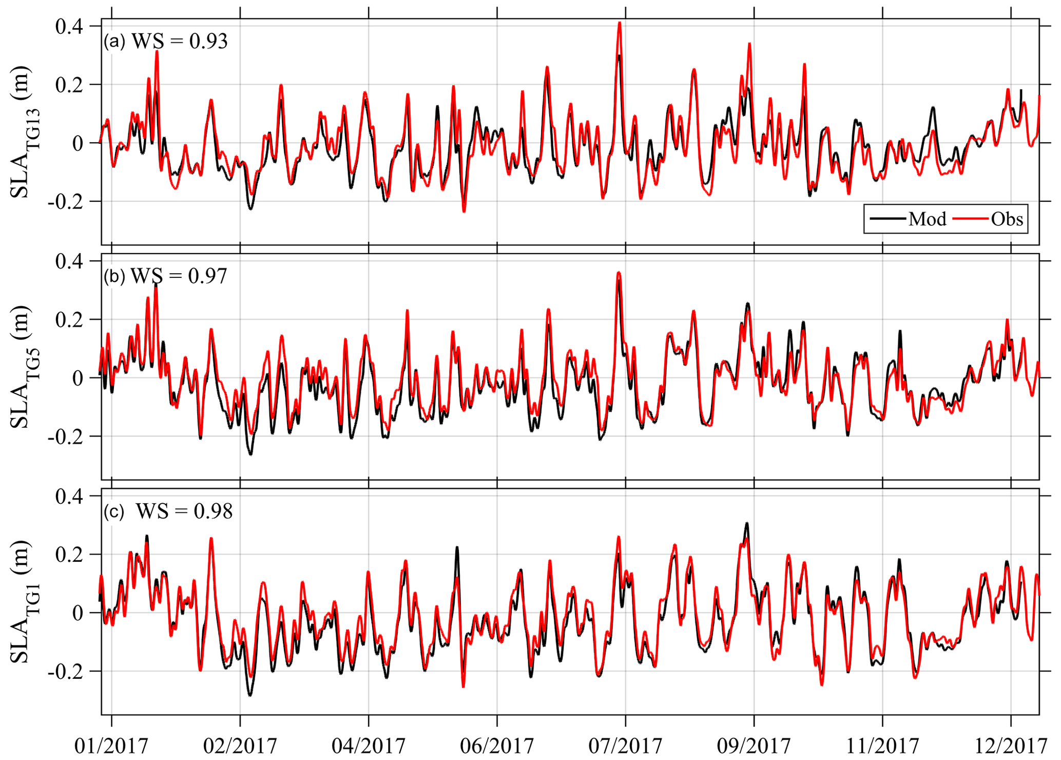
Figure 12 Observed (red) and modelled (black) sub-tidal anomalies of coastal sea level for calendar year 2017 at three stations: Manukau (SLA_TG13, a), Wellington (SLA_TG5, b) and Port Chalmers (SLA_TG1, c).

3.4.2 Coastal daily water temperature

Observed and modelled daily water temperature are compared over the hindcast period at 10 available temperature stations spanning the latitudinal range of New Zealand (Fig. 13, sites shown in Fig. 1). As for the SSH, the modelled values were extracted at the closest valid model grid point. At all stations, the seasonal cycle of temperature is large relative to other sources of variability. Differences in observed temperature between stations likely reflect a combination of the station latitude, exposure to the various boundary currents around New Zealand and that some coastal sampling stations are located in shallow bays or harbours. The length of the available observed time series for model–data comparison varies considerably with location (Table 3); therefore in this analysis primary statistics are presented for observations that overlap in time with the Moana Ocean Hindcast. This period varies in length from the entire hindcast period (e.g. Evans Bay and Portobello; Fig. 13g, i) to as little as a 4-year period at Bluff (Fig. 13j).

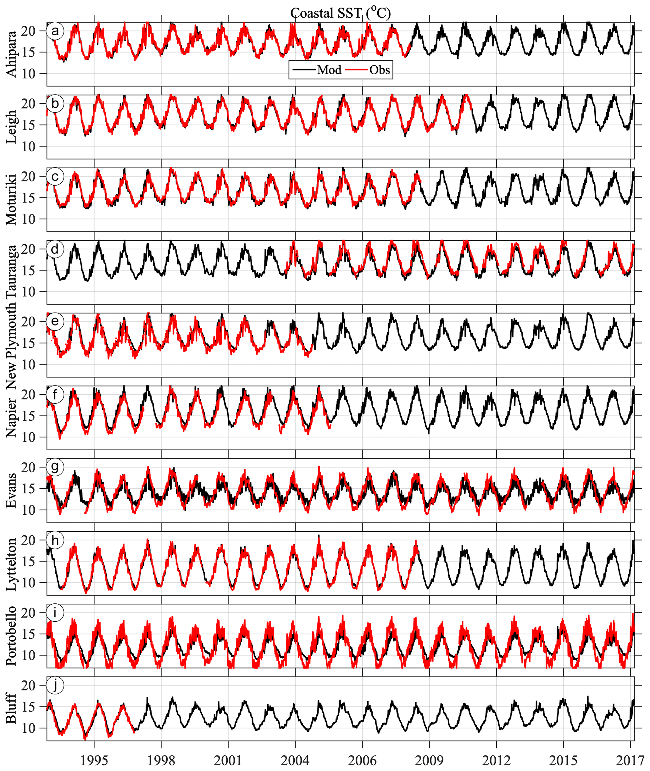
Figure 13 Observed (red) and modelled (black) daily coastal sea surface temperature from 10 stations around New Zealand (Table 3) roughly ordered from the northernmost (a, Ahipara) to southernmost (j, Bluff) station as shown in Fig. 1.

The primary time series statistics compared between observed and modelled temperature are the time mean, amplitude of the seasonal cycle, and the standard deviation of daily temperature anomaly σ_obs and σ_mod (Fig. 14). The anomaly is calculated as the difference between the raw daily individual time series and a harmonic regression fit consisting of the time mean, seasonal cycle and the first two higher harmonics of the seasonal cycle. The time-mean temperature at each station is very well reproduced by the model hindcast and is dominated by the north–south latitudinal gradient of the coastal temperature (Fig. 14a). The largest mean difference (bias) is a cold model bias found at the Tauranga wave buoy (−0.57 ^∘C, latitude −37.7^∘). Note that this measurement is taken from the base of a wave buoy (Table 3), a different method from the other stations. Due to a lack of wave buoy sampling during winter conditions, the Tauranga measurement is also slightly skewed towards summertime measurements.

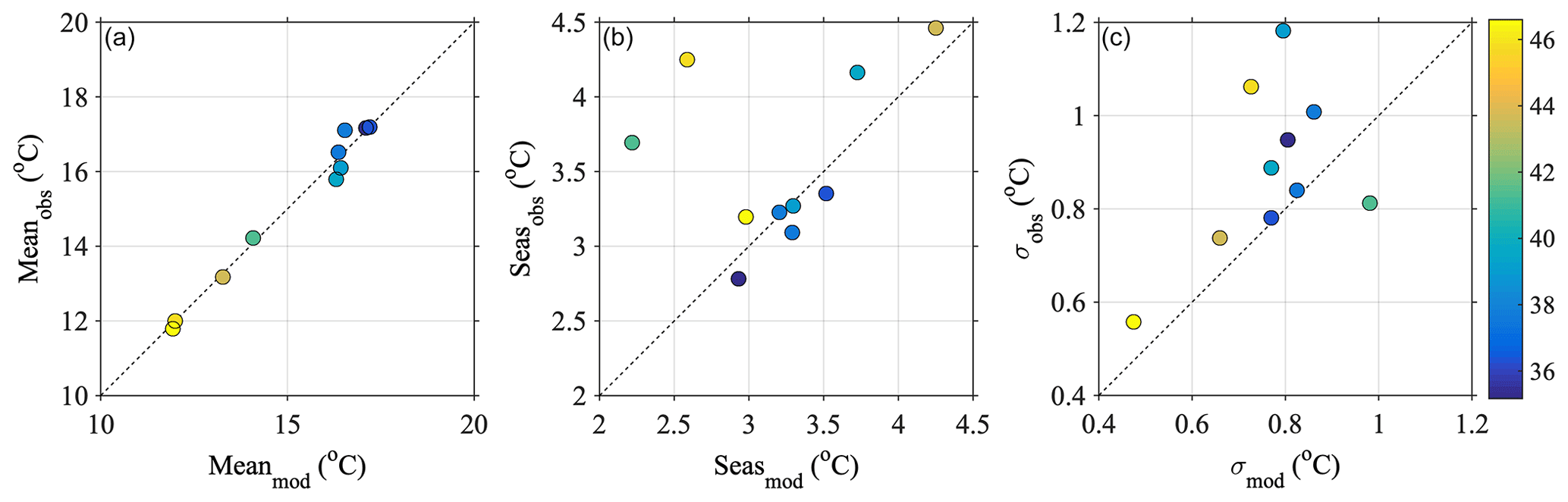
Figure 14 Primary statistics of coastal water temperature in the model (x axis) and observations (y axis): time-mean temperature (a), amplitude of seasonal harmonic (b) and standard deviation of daily temperature anomaly (c). Colours denote the latitude of the coastal measurement station location.

The amplitude of the seasonal cycle varies across station locations between 2–4.5 ^∘C, consistent with previous results (Chiswell and Grant, 2019). The amplitude of the modelled seasonal cycle falls within 0.25 ^∘C of a 1:1 line for 7 out of the 10 stations, with little discernible preference for latitude (Fig. 14b). This reflects cooler (warmer) temperatures at the peak of summer (winter) than observed at the coastal stations. The three stations with the largest discrepancy in seasonal cycle are all under-reproduced in the model. With the difference from 1:1 listed in descending order, these locations are Portobello (1.66 ^∘C), Evans Bay (1.47 ^∘C) and Napier (0.43 ^∘C). These locations are all located within semi-enclosed bays and harbours where a larger seasonal cycle can be observed but is potentially unresolved in a regional-scale oceanic model of this resolution due to land–air–sea processes. Satellite-derived annual cycle amplitudes show coastal regions around New Zealand vary from ≈3 ^∘C in northern New Zealand to about ≈1 ^∘C in southern New Zealand (e.g. Wijffels et al., 2018). The coastal annual cycles presented here are typically higher than the satellite-derived ones, consistent with previous analysis of coastal stations (Chiswell and Grant, 2019).

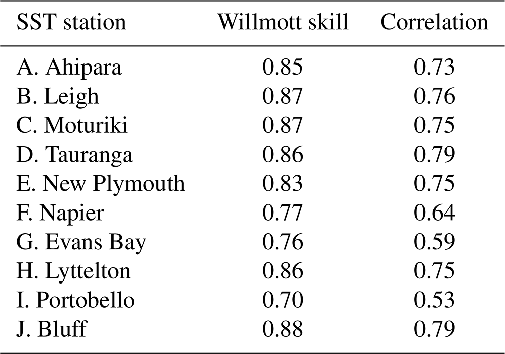
Non-seasonal, daily temperature anomaly variability ranges between 0.4–1.2 ^∘C in both the model and observations (Fig. 14c). At all locations, σ_obs is larger than σ_mod, except in Evans Bay, Wellington, which is not fully resolved by the 5 km grid spacing. Overall, these coastal temperature anomalies show a decrease with latitude in both observations and the model. In addition to the primary temperature statistics, the daily temperature anomaly time series are further compared with cross-correlation coefficients and Willmott skill (Eq. 4) between the model and observations. In general, both metrics are high and significant at the 95 % confidence level (Table 7), indicating that the processes regulating temperature anomalies at these stations are represented in the Moana Ocean Hindcast. Locations with somewhat lower correlations are similar to those with large differences in σ_obs compared to σ_mod (Fig. 14c).

Table 7 Coastal daily surface temperature model–data comparison statistics. Willmott skill is used as the model hindcast predictability metric. Pearson correlation coefficient is used as the degree of correspondence.

4 Conclusions

Our rigorous model evaluation shows that the Moana Ocean Hindcast provides a consistent, continuous and realistic representation of the ocean state around New Zealand. It includes important physical processes usually absent from global simulations, such as tides and the inverse-barometer effect, the contribution from all the main rivers, and a more detailed and realistic bathymetry. The results are available at higher spatial and temporal resolutions than most open-access datasets, providing an optimal basis for a series of analyses of the ocean dynamics in this region.

The model performs well in the coastal region as demonstrated by the comparison against coastal stations. The multi-decadal time frame of the simulation makes it useful for rigorous statistical analysis, including extreme value analysis necessary for coastal infrastructure projects. The simulation represents the ocean variability at a range of timescales from a few hours to inter-annual well. This makes the present configuration a good starting point for regional climate downscaling studies since it does not present intrinsic biases related to internal processes.

When compared to Souza et al. (2020), the present simulation shows an improvement in relation to the global reanalysis in the coastal region. The RMSE for the temperature and salinity profiles are comparable to the global models, even without data assimilation.

However, future improvements to the simulation could come from enhanced atmospheric forcing. Ideally, this would come from a built-for-purpose simulation, calibrated for the New Zealand region. The inclusion of variable river flux contribution is also a sensible point. It should be noted that the inter-annual variation of the flux can be more important than the seasonality. The inclusion of realistic river flux can lead to improvements of the model solution on the continental shelf.

Another way to make the model results more “realistic” is by data assimilation. This is part of the Moana Project, and a reanalysis is under development. A reanalysis, however, presents inherent discontinuities between assimilation windows, while a continuous free run provides an ideal data source for process studies.

Therefore, this first multi-decadal, high-resolution, open-access model represents a significant step forward for ocean sciences in New Zealand.