the Creative Commons Attribution 4.0 License.
the Creative Commons Attribution 4.0 License.
 | 13 Apr 2023
The Permafrost and Organic LayEr module for Forest Models (POLE-FM) 1.0
Winslow D. Hansen
Adrianna Foster
Benjamin Gaglioti
Rupert Seidl
Werner Rammer
Climate change and increased fire are eroding the resilience of boreal forests. This is problematic because boreal vegetation and the cold soils underneath store approximately 30 % of all terrestrial carbon. Society urgently needs projections of where, when, and why boreal forests are likely to change. Permafrost (i.e., subsurface material that remains frozen for at least 2 consecutive years) and the thick soil-surface organic layers (SOLs) that insulate permafrost are important controls of boreal forest dynamics and carbon cycling. However, both are rarely included in process-based vegetation models used to simulate future ecosystem trajectories. To address this challenge, we developed a computationally efficient permafrost and SOL module named the Permafrost and Organic LayEr module for Forest Models (POLE-FM) that operates at fine spatial (1 ha) and temporal (daily) resolutions. The module mechanistically simulates daily changes in depth to permafrost, annual SOL accumulation, and their complex effects on boreal forest structure and functions. We coupled the module to an established forest landscape model, iLand, and benchmarked the model in interior Alaska at spatial scales of stands (1 ha) to landscapes (61 000 ha) and over temporal scales of days to centuries. The coupled model generated intra- and inter-annual patterns of snow accumulation and active layer depth (portion of soil column that thaws throughout the year) generally consistent with independent observations in 17 instrumented forest stands. The model also represented the distribution of near-surface permafrost presence in a topographically complex landscape. We simulated 39.3 % of forested area in the landscape as underlain by permafrost, compared to the estimated 33.4 % from the benchmarking product. We further determined that the model could accurately simulate moss biomass, SOL accumulation, fire activity, tree species composition, and stand structure at the landscape scale. Modular and flexible representations of key biophysical processes that underpin 21st-century ecological change are an essential next step in vegetation simulation to reduce uncertainty in future projections and to support innovative environmental decision-making. We show that coupling a new permafrost and SOL module to an existing forest landscape model increases the model's utility for projecting forest futures at high latitudes. Process-based models that represent relevant dynamics will catalyze opportunities to address previously intractable questions about boreal forest resilience, biogeochemical cycling, and feedbacks to regional and global climate.
- Article
(12180 KB) - Full-text XML
-
Supplement
(313 KB) - BibTeX
- EndNote


The boreal forest is warming at a rate at least twice the global average (IPCC, 2021; Chylek et al., 2022), which can reduce fuel moisture and cause climate-sensitive disturbances, like forest fire, to increase (Seidl et al., 2020; Walker et al., 2020). Together, pronounced warming and larger, more severe fires are initiating abrupt changes in forest cover, structure, functions, and tree species composition (Johnstone et al., 2010a; Alexander and Mack, 2016; Walker et al., 2019; Mack et al., 2021; Baltzer et al., 2021), trends that will likely continue for at least the next several decades (Mekonnen et al., 2019; Foster et al., 2019, 2022). This is important because biophysical properties of the boreal forest underpin feedbacks to regional climate (Foley et al., 1994; Chapin et al., 2008; Rogers et al., 2013; Potter et al., 2020), and ∼ 30 % of all terrestrial organic carbon stocks are stored in the biome (Lorenz and Lal, 2010; Schurr et al., 2018). Some portion of those stocks could be released to the atmosphere and further accelerate warming (Anderegg et al., 2022). Thus, society urgently needs projections of where, when, and why the boreal forest will change.
Ecological legacies are the organismal adaptations (i.e., information), physical materials, and energy that persist in ecosystems through multiple disturbances (Ogle et al., 2015). Legacies will underpin how the boreal forest responds to climate change and fire (Turetsky et al., 2016; Johnstone et al., 2016). For example, adaptive traits, like cone serotiny (cones that stay closed for many years until heated by fire) and asexual resprouting, are information legacies that facilitate postfire forest recovery (Johnstone et al., 2009, 2010a). Thick moss-dominated soil-surface organic layers (SOLs) form over decades of postfire forest development, and a portion often escapes burning in the subsequent fire, leading to accumulation of SOL over multiple fire cycles (Walker et al., 2018). This serves as a physical legacy that preserves permafrost (subsurface material that remains frozen for at least 2 consecutive years) (Kasischke and Johnstone, 2005; Jorgenson et al., 2010) and shapes tree species composition by controlling seedling germination and establishment (Johnstone et al., 2020). In conjunction with insulative physical legacies, energy legacies of past temperature regimes also maintain permafrost underneath forests where current air temperature would otherwise not support it (Schuur and Mack, 2018).
Physical and energy legacies underpin spatio-temporal patterns of permafrost at multiple scales. In the boreal forest of North America, permafrost is continuous in the north, becomes discontinuous and sporadic, and is then eventually absent in the south (Obu et al., 2019). Within the discontinuous zone, the permafrost distribution is heterogeneous, varying on fine spatial scales with topography, dominant forest type, and fire history (Brown et al., 2016; Gibson et al., 2018). Permafrost dynamics are particularly important for shaping boreal forest structure and function as well as hydrology (Turetsky et al., 2010; Baltzer et al., 2014; Dearborn and Baltzer, 2021). Within permafrost-affected soils, a portion of the soil column termed the “active layer” undergoes an annual cycle of freezing and thawing. The annual maximum active layer depth can vary from a few centimeters to several meters (Smith et al., 2022). This freezing-and-thawing cycle determines the seasonality, vertical distribution, and amount of plant-available soil water and influences nutrient availability (Abbott and Jones, 2015; Young-Robertson et al., 2017).
In response to continued warming, annual maximum active-layer depth is predicted to increase, and the distribution of permafrost will likely contract, with large hydrologic and biogeochemical consequences (Pastick et al., 2015; Schuur and Mack, 2018). Increasing wildfire (Veraverbeke et al., 2017; Phillips et al., 2022) will also impact permafrost by combusting SOLs and altering tree regeneration pathways (Baltzer et al., 2021; Johnstone et al., 2010a). However, permafrost and the legacies that affect its dynamics are rarely considered in forest models. In fact, just a handful of models explicitly simulate permafrost (Foster et al., 2019; Gustafson et al., 2020; Kruse et al., 2022), and those that do often operate at relatively coarse spatial (≥ 25 ha grid cells) and/or temporal (≥ monthly) resolutions (but see Kruse et al., 2022, who describe a permafrost module that runs with a 5 min temporal resolution). This makes it difficult to capture the fine-scale spatial heterogeneity of permafrost distributions and the effects of daily temperature variability on plant water availability during short but critical shoulder seasons. Further, most existing permafrost algorithms rely on computationally intensive numerical methods (Sitch et al., 2003; Beer et al., 2007; Karra et al., 2014; Perreault et al., 2021; Yokohata et al., 2020; Westermann et al., 2016), limiting the spatio-temporal resolutions at which they can be applied, particularly across broad domains.
To address this challenge, we present the Permafrost and Organic LayEr module for Forest Models (POLE-FM) that was designed to mechanistically simulate daily changes in active layer depth, annual SOL accumulation, and the associated ecological effects on boreal forests and fire at a fine spatial resolution (i.e., grain of ∼ 1 ha) in a computationally efficient manner (Fig. 1). When paired with a state-of-the-art forest model, such as iLand, the module allows for simulation of complex feedbacks among forests, fire, and permafrost dynamics in topographically complex landscapes under historical and future conditions. In this paper, we describe the module and benchmark its ability to represent permafrost and SOLs in forest stands to landscapes of interior Alaska across days to centuries.
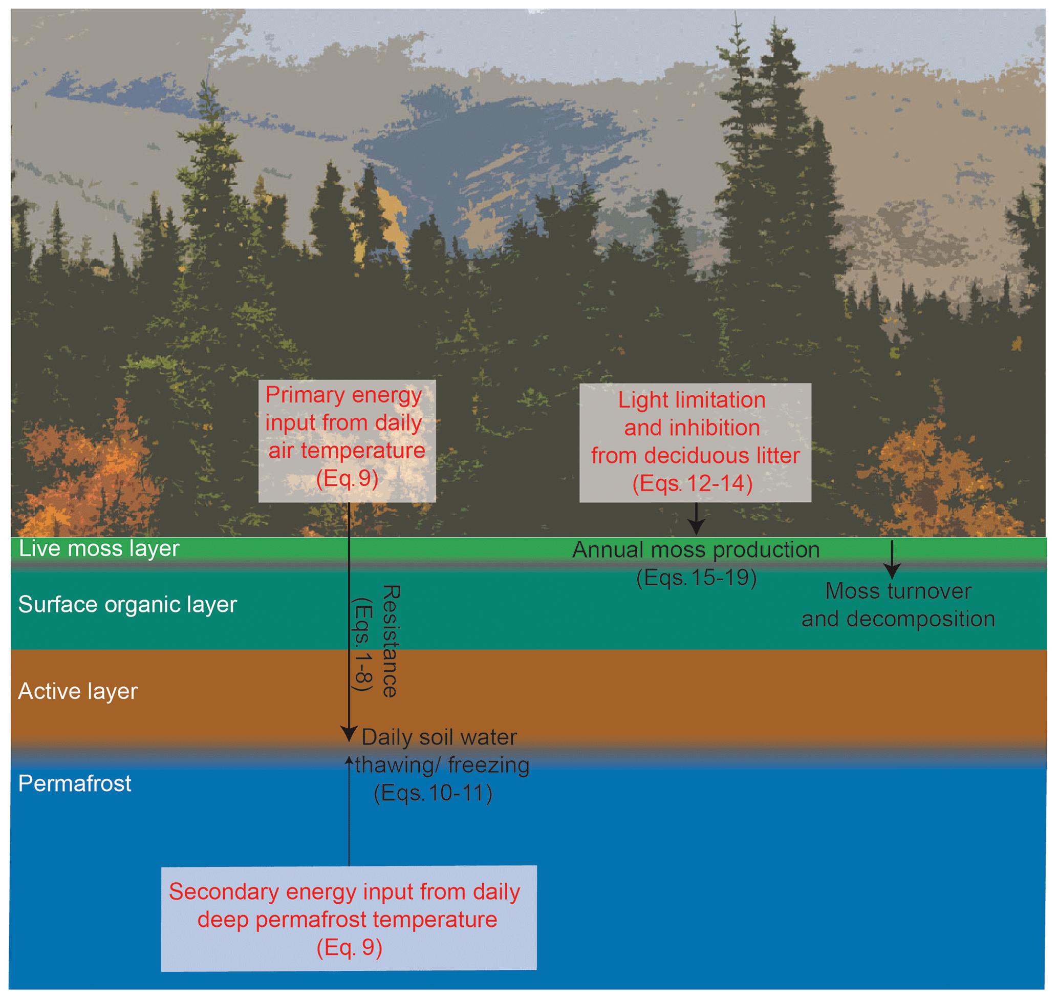
Figure 1Conceptual diagram of the permafrost and soil-surface organic layer module. State variables are in white, processes are described in black, and forcing variables are in red.
2.1 Permafrost and SOL module
The module represents daily changes in active layer depth and long-term trends (years to decades) in permafrost presence. Permafrost is represented based on physical principles of heat transport through vegetation and soil media with varying thermal resistances affected by soil moisture content. We incorporate the insulating effects of snow and deep SOLs and capture transient shifts between permafrost regimes (e.g., a transition from temporally continuous to sporadic permafrost due to climate change). Moreover, we aimed for a computationally efficient approach that operates well within the runtime and memory constraints of forest models. The module tracks the energy fluxes that thaw and freeze water at the edge of the active layer (zero isoline, or the depth at which soil temperature is 0 ∘C), requires only a few state variables, and provides daily values of active layer depth with little computational overhead by avoiding iterative numerical approximations of differential equations.
To capture daily changes in active layer depth, we first estimate the thermal resistances R (m2 W−1 K−1) of snow (when present), SOL, and the mineral soil layer (Eq. 1).
Snow depth is represented as a function of the precipitation that falls during days with mean air temperature below 0 ∘C and the density of snowpack (set at 190 kg m−3) (Bonan, 1991; Bennett et al., 2019). We set snow thermal conductivity, Snow.k, at 0.3 W m−1 K−1 (Cook et al., 2008). SOL depth is estimated based on the mass of live and dead mosses and litter pools in each grid cell. SOL thermal conductivity, SOL.k, is set at 0.09 W m −1 K−1 (Hinzman et al., 1991; O'Donnell et al., 2009).
Characteristics of the mineral soil layer that determine its conductivity are explicitly considered. We allow mineral soil thermal conductivity, M.Soil.k, to vary with soil texture and soil moisture. We derive mineral soil conductivity following the approach of Farouki (1981) as described in Bonan (2019) (Eq. 2).
where M.Soil.k is determined by linearly ramping between saturated conductivity, M.Soil.k.sat, and dry conductivity, M.Soil.k.dry, based on a factor, Ke, that varies with relative soil moisture and soil texture, represented separately for unfrozen (Eq. 3) and frozen (Eq. 4) soils.
where Ke is the Kersten number, and SE is the volumetric soil water content (VWC) relative to the volumetric soil water content at saturation (VWC.sat).
M.Soil.k.dry is estimated from bulk density (Eq. 5).
where . M.Soil.k.sat is estimated as a function of the conductivity of solids, water, and ice in the matrix, modeled separately for unfrozen (Eq. 6) and frozen (Eq. 7) soils.
We assume Kwater =0.57 and Kice = 2.29 W m−1 K−1. Calculation of Ksolid is calculated in Eq. (8).
Using the total thermal resistance R from Eq. (1), we can then estimate the daily sum of energy flow (Einput, MJ d−1) that reaches the zero isoline from the atmosphere above (Eq. 9).
where Air.Temp is the daily mean air temperature, Temp.zero.isoline = 0 ∘C, and the constant converts from J s−1 to MJ d−1. Einput is then used to calculate the daily sum of water that thaws or freezes at the zero isoline based on the enthalpy (or latent heat) of fusion (Ethaw; 0.33 MJ L−1 water). Equation (9) is also used to estimate the daily energy flux from soil below the active layer by replacing Air.Temp with the temperature of the soil below. Deep soil temperatures, set at 5 m, are assumed to be at equilibrium with mean annual air temperature of the previous decade (Riseborough, 2004).
We then model the daily amount of water that thaws or freezes, delta.W.mm (Eq. 10).
where delta.W.mm is constrained to values between −10 and +10 mm (only 10 mm of water is allowed to freeze or thaw each day in order to avoid numerical instabilities close to the soil surface). Finally, the corresponding depth of soil that freezes or thaws each day in meters, delta.s.m, is calculated (Eq. 11).
Since frozen soil (and the water captured therein) is not accessible for plants, the actual water holding capacity of the soil is dynamically modified each day. If soil thaws in a given day, that freshly melted water is added to the soil water pool and the capacity for soil to hold water increases. The approach described here also works for estimating seasonal thawing and freezing of soils in areas not underlain by permafrost.
The SOL component was adapted from Bonan and Korzuhin (1989) and Foster et al. (2019) and represents SOL depth as a function of annual moss net primary production, biomass accumulation, respiration, and turnover. It adds live and dead moss to the fuels for forest fires, and the depth of the SOL influences postfire tree regeneration. Annual moss productivity is simulated as a function of environmental scalars that represent effects of light attenuation through the forest canopy and moss layer and growth inhibition from fresh deciduous litter. The amount of light that reaches moss for photosynthesis attenuates with increasing forest canopy cover and with increasing moss biomass. Effects of light attenuation are represented by first calculating the amount of light available for photosynthesis in year t as Light.availt (Eq. 12).
where k is the light extinction coefficient, set at 0.92, LAI.forestt is the leaf area index (square meters of leaf area per square meter of ground) of tree cover in year t. LAI.mosst is the leaf area index of moss in year t calculated as moss biomass multiplied by the specific leaf area of moss (1 m2 kg −1) (Foster et al., 2019, and https://github.com/UVAFME/UVAFME_model/blob/main/src/Soil.f90, last access: 10 October 2022). The effect of light attenuation on moss productivity, FLight.availt, is then calculated (Eq. 13).
where LRmax is the light saturation point, or the amount of light, relative to the light level above the canopy, above which an increase in light does not increase moss gross primary production (GPP), set at 0.05. LRmin is the light compensation point, or the amount of light, relative to light level above the forest canopy, beyond which moss begins to photosynthesize, set at 0.01.
Field experiments show that fresh leaf litter from deciduous broadleaf tree species strongly inhibits moss productivity (Jean et al., 2020). Such inhibitory effects, FDecidt, are modeled as Eq. (14).
when or 1 when , where is the fresh (previous year's) forest floor deciduous litter biomass in megagrams per hectare. At, annual assimilation by moss in year t (kilograms of biomass per square meter of leaf area) is then computed (Eq. 15).
where AMax, the maximum moss productivity per unit leaf area, is 0.3 kg m−2 yr −1 (Foster et al., 2019). We estimate effective assimilation in year t, A.efft, in kilograms per kilogram biomass (Eq. 16).
Moss productivity in year t, Pt, in kilograms per square meter biomass then depends on turnover, Tt, and respiration, Rt, in year t (Eqs. 17–19).
where is the previous year's moss biomass in kilograms per square meter, and b and q are empirical parameters set at 0.136 and 0.12, respectively (Foster et al., 2019). The moss biomass pool is updated (Eq. 20).
Note that the biomass pool can shrink if Pt becomes negative, e.g., due to a closing canopy.
Thickness of the live moss layer is calculated as biomass divided by a bulk density of 31 kg m−3 calculated from field observations described in Walker et al. (2020). Dead moss and forest floor litter layer thickness is calculated as biomass divided by bulk density, set at 91 kg m−3 (Walker et al., 2020).
The permafrost and SOL module is implemented in C for computational efficiency and is relatively compact (< 1000 lines of code). It is compatible with PC, Linux, or Mac, and full source code and documentation are available under a GNU General Public License (GNU GPL http://www.gnu.org/licenses/gpl-3.0.html, last access: 1 October 2022) (see code availability section). While the design is modular, we note that the complex feedbacks between vegetation, permafrost dynamics, and SOL accumulation may require some adaptations and code modifications when integrating our work in different forest models. Below, we detail the integration into the individual-based forest landscape and disturbance model iLand (Seidl et al., 2012a).
2.2 Coupling the permafrost and SOL with iLand
The growth and mortality of individual trees in spatially explicit landscapes are simulated by iLand as a function of canopy light interception, climate, nutrient availability, and disturbance (Seidl et al., 2012a, b). The model was originally designed to study effects of natural disturbances, like forest fire, on forest landscapes in the context of climate change (Seidl et al., 2012a). Thus, iLand emphasizes representation of disturbances and the processes that underpin forest responses to disturbance, including tree seed production and dispersal, abiotic filters of tree seedling establishment, and multiple pathways of tree mortality (Seidl et al., 2012a, b; Hansen et al., 2018, 2020). For an exhaustive technical description of iLand, including carbon cycling and simulation of forest fire, see Appendix A and https://iland-model.org/ (last access: 1 October 2022), which includes full model source code.
The proportion of moss biomass that turns over (dies) each year in the new module is fed into the litter layer of iLand's decomposition module. Decomposition is simulated by iLand as a function of climate and pool-specific carbon-to-nitrogen ratios (Seidl et al., 2012b). The C:N ratio of moss litter is set at 30 (Melvin et al., 2015). Together, live moss, dead moss, and forest floor litter layers comprise the SOL in iLand. Wildfire ignition, spread, and severity are partially contingent on downed fuel availability in iLand (Seidl et al., 2014a), and we now include live and dead moss as available fuel in the fire module. When a grid cell burns, the combusted forest floor litter, dead moss, and live moss pools are subtracted from SOL depth.
The tree species that establish in years following fire shape multi-decadal successional trajectories (Seidl and Turner, 2022). The depth of burning in the SOL is an important determinant of seedling establishment success because the SOL is often dry, and seedlings must expand their roots into mineral soil to access water (Johnstone and Chapin, 2006; Brown and Johnstone, 2012). We therefore included the effect of deep SOL as an additional limiting factor when calculating tree seedling establishment in iLand. For each 1 ha iLand cell, the probability of establishment is scaled with a negative exponential function following Trugman et al. (2016) (Eq. 21).
where estab.pt is a multiplicative factor reducing the abiotic establishment probability in year t; SOL.deptht is the depth of the SOL (cm) in year t; and c is a species-specific shape parameter, set at 0.50 for trembling aspen (Populus tremuloides Michx.) and Alaskan birch (Betula neoalaskana Sarg.), 0.25 for white spruce (Picea glauca (Moench) Voss), and 0.15 for black spruce (Picea mariana (P. Mill.) B.S.P.).
We used a pattern-oriented modeling framework (Grimm et al., 2005) to evaluate the new module by simulating forests of interior Alaska at stand and landscape scales over days to centuries. Pattern-oriented modeling is an approach to benchmarking where patterns of many variables operating at multiple temporal and spatial scales are compared to observational datasets. We chose interior Alaska because it is located in the discontinuous permafrost zone where permafrost presence, moss production, and SOL accumulation vary with dominant forest type, disturbance history, and topography. For example, areas dominated by mature black spruce in lowland valley bottoms and north-facing slopes are generally underlain by permafrost and support a relatively productive forest floor moss layer and thick SOLs. Upland and south-facing slopes are dominated by deciduous trembling aspen and Alaskan birch, which are often not underlain by permafrost, and moss is far less prevalent. White spruce also inhabits upland positions on its own or mixed with black spruce and contains SOLs of intermediate thickness (Van Cleve and Viereck, 1981). The multiple interacting biotic and abiotic drivers of permafrost and moss productivity create complex landscape mosaics (Johnstone et al., 2010a) that we wanted to ensure the module could produce.
We first evaluated whether the module could generate reasonably realistic daily patterns of snow accumulation/melting and active layer thawing/freezing at the stand level. We then simulated a ∼ 61 000 ha forested landscape to test whether the approach could generate complex mosaics of near-surface permafrost presence, moss productivity, and SOL accumulation consistent with observations. To ensure robust simulations, we updated an existing iLand tree species parameter set for interior Alaska (Hansen et al., 2021) (Table B1) and parameterized the iLand carbon cycle (Table B2) using values derived from the literature.
3.1 Temporal patterns of snow and active layer depth
To evaluate whether the module could generate realistic intra- and inter-annual patterns of snow accumulation and active layer depth, we selected 17 forested sites in interior Alaska that span approximately 700 km. The southernmost site sits along the Alaskan highway at the border between Canada and Alaska. The northernmost site is just south of the Brooks mountain range along the Dalton highway. Each site was instrumented with temperature probes to measure daily soil temperature at depths of 0 to 6 m between 2014 and 2018 (https://permafrost.gi.alaska.edu/sites_list, last access: 1 March 2022). Seven of the sites were recorded as having an annual maximum active layer depth of less than 2 m (permafrost present). Ten of the sites had an annual maximum active layer deeper than 2 m (permafrost absent). We used the 2 m depth cutoff because it is the maximum effective soil depth assumed in iLand. The sites were initialized from field inventories covering the same domain selected to match the species composition recorded in the soil temperature database (Walker and Johnstone, 2014; Johnstone et al., 2020). Soil information used to initialize iLand was extracted from the global SoilGrids250m V. 1.0 (for effective soil depth) and 2.0 (for percent sand, silt, and clay) (Hengl et al., 2017). Relative soil fertility, expressed as plant-available nitrogen, was set to 45 kg ha−1 yr−1 (Hansen et al., 2021). Depth of the SOL was not recorded in the soil temperature database for the 17 sites. Thus, we used photos from the instrumented sites and information on the dominant forest type to assign initial SOL depths to the iLand stands. Sites where researchers recorded dominance of deciduous trees or where SOLs appeared absent or shallow in photographs were assigned a depth of 0 or 0.07 m to match independent field estimates of SOL depths in deciduous forests located in the Tanana Valley near Fairbanks (Melvin et al., 2015). Sites dominated by black spruce or where photographs suggested a deep SOL were assigned a depth of 0.25 m based on field surveys of black spruce stands (Johnstone et al., 2010a). Stands dominated by white spruce were assigned an intermediate depth of 0.16 m.
Stands were simulated in iLand with 2001–2018 daily climate (minimum and maximum daily temperature, precipitation, shortwave solar radiation, and vapor pressure deficit) from the 1 km Daymet product (Thornton et al., 2021). We benchmarked simulated maximum annual snow depth and timing of snowmelt for the period 2001–2017 (the period when snow observations were available) using a gridded snow product (Yi et al., 2020). This product was developed by integrating downscaled reanalysis data with satellite imagery to provide a continuous estimate of snow depth at 1 km spatial grain. When compared with a meteorological station network (SNOTEL), the gridded observational product had a RMSE of 0.32 m with a bias of −0.09 m in mid-elevations (400–800 m), where 70 % our forested sites were located, and a bias of 0.01 m at low elevations (< 400 m), where the rest of our sites were located (Yi et al., 2020).
We compared simulated and observed maximum annual active layer depth for 2014–2018, the period where soil temperature observations were available, at the 7 permafrost sites and maximum annual freezing depth for the 10 non-permafrost sites. We converted observed daily soil temperatures at depths of 0.03, 0.5, 1, 1.5, 2, 4, and 6 m to active layer depth by identifying the zero isoline with linear interpolation. We also compared the day of year when maximum active layer depth and freezing depth were reached in simulations and observations.
3.2 Landscape heterogeneity in near-surface permafrost presence, moss productivity, and SOL accumulation
We evaluated whether the module, coupled with iLand, could simulate landscape mosaics of near-surface permafrost (≤ 1 m deep), moss production, and SOL accumulation in a large forested area (∼ 61 000 ha of land area). We initialized the model with a tree species composition map based on a remotely sensed plant functional type (PFT) product for Alaska and western Canada that classified vegetation as spruce, deciduous, mixed forest, or nonforest (Wang et al., 2020) and reflected fire history. We further decomposed PFTs into black spruce, white spruce, trembling aspen, Alaskan birch, mixed forest, potential forest (i.e., areas currently unforested that could support forest in the future), and nonforest using rules based on aspect, elevation, and a permafrost map (Table B3). While this approach allowed us to disaggregate PFTs to the species level, we lack robust datasets to evaluate the accuracy of the species composition map. This is a challenge as the dominant tree species determines SOL accumulation and permafrost distribution. In the future, well-validated, remotely sensed tree species composition maps would markedly reduce initial condition uncertainty in forest simulations in interior Alaska (Hermosilla et al., 2022).
Initial stand densities, tree sizes, and forest floor carbon pools (litter, coarse wood, live and dead moss; Table B4) for the appropriate tree species were initialized in the model as early postfire (11 years old) forest based on field inventories described earlier (Walker and Johnstone, 2014; Johnstone et al., 2020). Because the forest landscape was initialized as entirely early postfire, it did not reflect variation in forest stand age. Thus, we ran a 200-year spin-up as a function of historical climate (climate years 1950–2005 recycled randomly with replacement) and simulated fire dynamically to generate spatial heterogeneity consistent with internal model logic, following protocols established in previous iLand studies (Hansen et al., 2020; Turner et al., 2022). We then simulated forests for another 100 years and used this period in all analyses.
We want to eventually conduct simulations with future 21st-century climate. Thus, we used daily meteorological data from the historical period of the CMIP5 generation CCSM4 general circulation model (GCM) (Gent et al., 2011) to force landscape-level simulations instead of Daymet (as was used in the stand-level experiment). This GCM corresponds closely with observed historical climate in Alaska (Walsh et al., 2018), and we statistically downscaled it to a 1 km spatial resolution using quantile matching with Daymet as the observational grid (Hansen et al., 2021). We extracted soil data from the same sources as the stand-level experiment that geographically corresponded to the 1 ha grid cells in our simulated landscape. Because fire is stochastic in iLand and an important determinant of permafrost dynamics, SOL depth, tree species composition, and stand structure, we ran 10 replicates and analyzed output from the run with the smallest difference between modeled and observed mean annual burned patch size and annual probability of a fire event.
We compared fire from simulation years 201–300 to observations in the Alaska Large Fire Database from the period 1980–2021. This database contains perimeters for larger fires (size threshold for inclusion has varied over time, ranging from 10–1000 ha) and point locations for smaller fires in Alaska. We chose years 201–300 for evaluation because a century aligns with the historical-mean fire return interval in Alaska (Johnstone et al., 2010b). We combined these datasets to ensure comprehensive coverage and assumed a circular shape for the smaller fires when perimeters were unavailable. Fire is a stochastic process in iLand, so we did not expect perfect correspondence between modeled and observed individual fire sizes and locations. Instead, we aimed for the model to generate fire characteristics (i.e., frequency, patch size, annual area burned, and severity) that were generally consistent with the observational record. We took two approaches for benchmarking. First, we compared simulated and observed annual probability of fire occurrence and mean annual burned patch size, as well as the proportion of stems and basal area killed by fire. Second, we compared simulated and observed fire characteristics from the landscape with observed fire characteristics in all of the forests of interior Alaska broken into 625–61 000 ha landscapes. This allowed us to determine how the dynamic fire module in iLand performed for our landscape specifically and how the model performed relative to the spatial variation in fire regimes across interior Alaska.
We compared the proportion of the landscape underlain by near-surface permafrost in the last 40 years of simulation (years 261–300) to a remotely sensed product of near-surface permafrost presence (Pastick et al., 2015). Forty years was chosen because we wanted to evaluate permafrost over a multi-decadal period and because it aligned with the period used to evaluate postfire SOL combustion and tree seedling density (see below). This product was created by integrating satellite records and other geospatial datasets to predict the probability of near-surface permafrost presence at a 30 m spatial resolution with machine learning. Because iLand operates at 1 ha spatial resolution for permafrost, we aggregated the remotely sensed data from 30 m to 1 ha grid cells by calculating the mean probability of near-surface permafrost presence in each 1 ha grid cell. We then used a ≥ 50 % probability of permafrost presence, the same cutoff used in the original analysis (Pastick et al., 2015), to map the permafrost distribution. In iLand, near-surface permafrost was considered present in any grid cell where the annual maximum active layer depth was ≤ 1 m in 15 (38 %) of the last 40 years of simulation. This cutoff ensured we only included areas that were underlain by consistently frozen ground. We compared the total proportion of the landscape underlain by near-surface permafrost and how permafrost presence varied as a function of aspect in simulations and the benchmarking product. We also evaluated how permafrost presence varied as a function of simulated dominant tree species but did not compare to the benchmarking product because we lack tree species composition maps in interior Alaska.

Figure 2(a) Observed vs. simulated maximum annual snow depth at 17 sites between 2001–2017. (b) Observed vs. simulated day of spring snowmelt at 17 sites between 2001–2017. (c) Observed vs. simulated maximum annual thaw depth at seven sites underlain by permafrost between 2014–2018 (only site years with complete observational records are included). (d) Observed vs. simulated maximum annual freeze depth at 10 sites not underlain by permafrost between 2014–2018 (only site years with complete observational records are included). Black lines show one-to-one relationships in all panels.
We compared SOL carbon in simulation year 300 separated by forest type to field inventories (Alexander and Mack, 2016; Walker et al., 2020). While benchmarking data were unavailable, we also evaluated landscape variability in total SOL and live moss depth. We assessed SOL combustion by fire in different forest types for model years 261–300 and compared model output to the two extensive sets of postfire field plots (Walker and Johnstone, 2014; Johnstone et al., 2020; Walker et al., 2020) also used for initialization. The period of analysis was selected to ensure a sufficient number of fires while balancing the computational intensity of these calculations.
Because near-surface permafrost presence and moss productivity are affected by and feed back to influence forest dynamics, we determined whether the model could realistically represent landscape-level patterns of tree species composition and stand structure. We explored how landscape patterns of dominant forest type shifted through 300 years of simulation and compared simulated stand density and basal area of each forest type from the end of the simulation with two field inventories. The first was a regional network of permanent plots in interior Alaska collected by the Bonanza Creek Long-Term Ecological Research Network (Ruess et al., 2021). The second inventory was the Cooperative Alaska Forest Inventory, which is a set of permanent plots covering interior Alaska, south-central Alaska, and the Kenai Peninsula (Malone et al., 2009). We reran the 300-year simulation with the SOL and permafrost module turned off to evaluate how the module shaped landscape distributions of tree species composition.
We also compared simulated aboveground live tree biomass from the end of the simulation with remotely sensed estimates of aboveground live woody biomass for interior Alaska and western Canada (Wang et al., 2021). This dataset is a 30 m product that characterizes annual live woody biomass for the years 1984–2014. We aggregated 2014 biomass estimates to the 1 ha spatial resolution of iLand using bilinear interpolation. We further benchmarked snag and coarse-wood carbon pools in model year 300 with published field observations (Alexander and Mack, 2015; Melvin et al., 2015).
To quantify the underpinning drivers of landscape variability in tree species composition and aboveground live and dead biomass, we compared simulated variation in postfire tree seedling density by species and SOL depth from years 261–300 with field observations (Walker and Johnstone, 2014; Johnstone et al., 2020) using the same fires that were analyzed for postfire SOL combustion. Finally, we analyzed the computational efficiency of the module by simulating the landscape with and without the permafrost module turned on to quantify its memory requirement and runtime.
Dominant forest type was determined using species importance values (IVs), a measure of stand dominance based on the relative proportions of species density and basal area. It ranges from zero to two (Hansen et al., 2020). We considered stands dominated by a particular species if their IV was greater than one. Stands were considered mixed spruce or mixed deciduous forest if black spruce and white spruce or aspen and birch IVs summed to greater than one, respectively. Averages in the text are presented as medians and inter-quartile ranges (IQRs) (25th–75th percentiles). When comparing simulated and observed datasets, parametric statistics were not used because sample sizes can be increased with simulations to artificially inflate statistical significance. Benchmarking analyses were conducted in R statistical software V. 4.0.4 (R Core Team, 2021) using the packages tidyverse (Wickham et al., 2019) and terra (Hijmans, 2021).
4.1 Snow depth, timing of snowmelt, and active layer depth
When forced with 2001–2017 climate, median simulated maximum annual snow depth was 0.68 (0.52–0.84) m compared with median observed maximum annual snow depth of 0.49 (0.39–0.59) m. The model overestimated snow depth for sites and years where snowfall was above average (Fig. 2a), likely because snow compaction is not considered in the model. The simulated median number of Julian days to snowmelt was 122 (116–130) compared to the observed median number of Julian days of 117 (117–125) (Fig. 2b).
When forced with 2014–2018 climate, simulated median annual maximum active layer depth was 1.6 (1.3–1.8) m, and observed median annual maximum active layer depth was 1.4 (1.0–1.5) m in seven forest stands underlain by permafrost (Fig. 2c). Simulated daily patterns of active layer depth also corresponded well with observations (Fig. 3). On average, maximum annual active layer depth occurred 20 d later in iLand than in observations with an IQR of 10 d earlier to 39 d later. Simulated and observed median annual maximum freezing depths were 2.0 (1.9–2.0) m and 1.9 (1.9–2.0) m, respectively (Fig. 2d). On average, the maximum annual freeze depth was reached 10 d earlier in simulations than in observations with an IQR of 28 d earlier to 7 d later than observations.
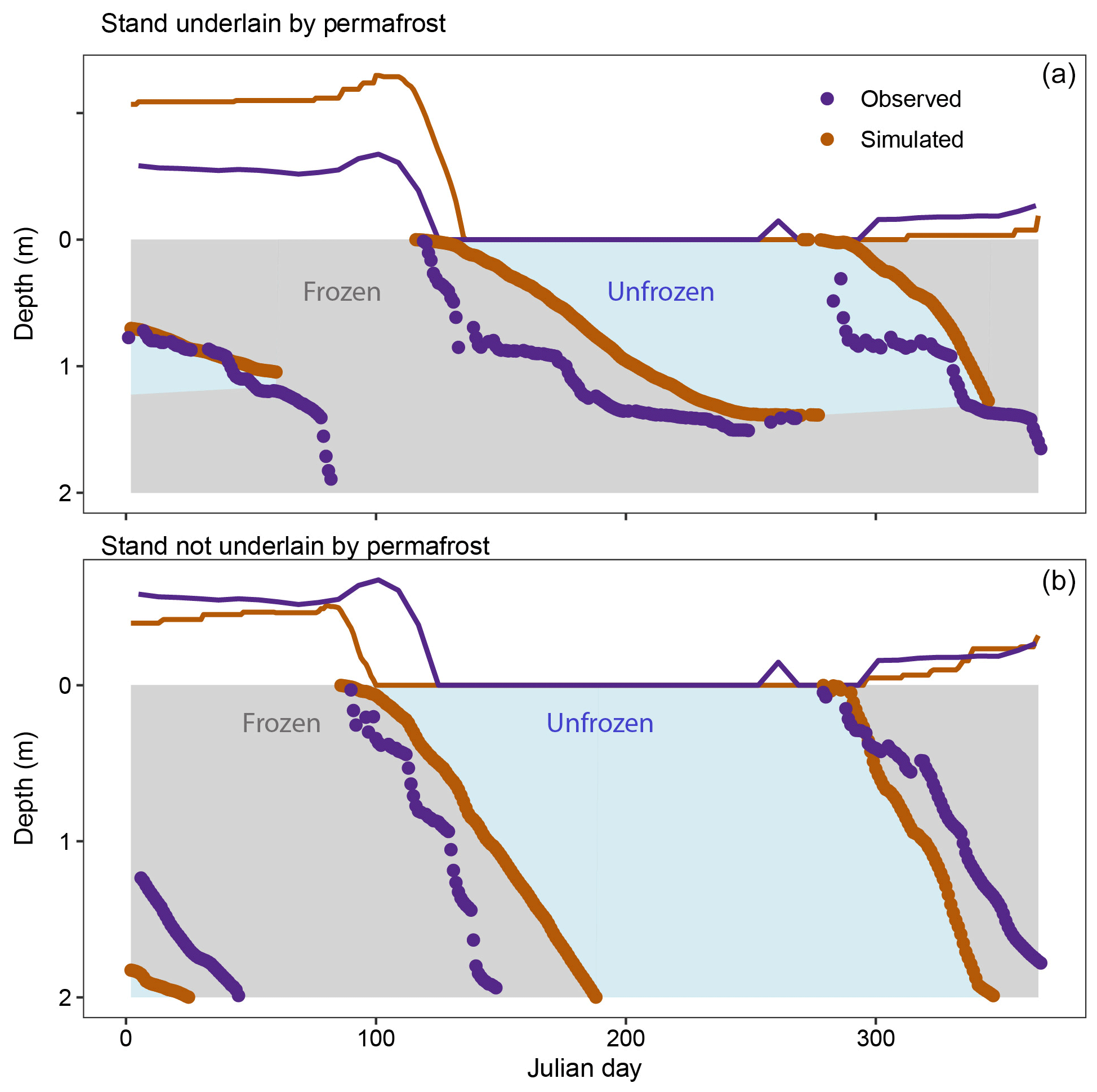
Figure 3(a) Example of daily active layer freezing and thawing. Data from 2016 at one of seven forest stands underlain by permafrost. (b) Example of daily thawing and freezing. Data from 2016 at 1 of 10 forest stands not underlain by permafrost. Solid lines represent snow depth. Dots represent active layer depth or depth of freezing. Gray fill represents simulated frozen soils. Blue fill represents simulated unfrozen soils.
4.2 Landscape-level fire characteristics
Mean annual burned patch size was 3628 ha, and annual probability of a fire event was 11 % in the best of the 10 replicate landscape simulations. These values differed from observed values by 5 % and 8 %, respectively (Fig. 4a, b). However, among all 10 replicates, burned patch size and probability of a fire event differed by as much as 44 % and 42 %, highlighting the stochastic nature of fire. Both observed and simulated fire metrics for the landscape were also representative of observed fire characteristics in all 625 sampled 61 000 ha landscapes across the boreal domain of Alaska (Fig. 4c). On average, 73 (70–76) % of stems and 52 (46–60) % of basal area were killed by fire in the model (Fig. B1).
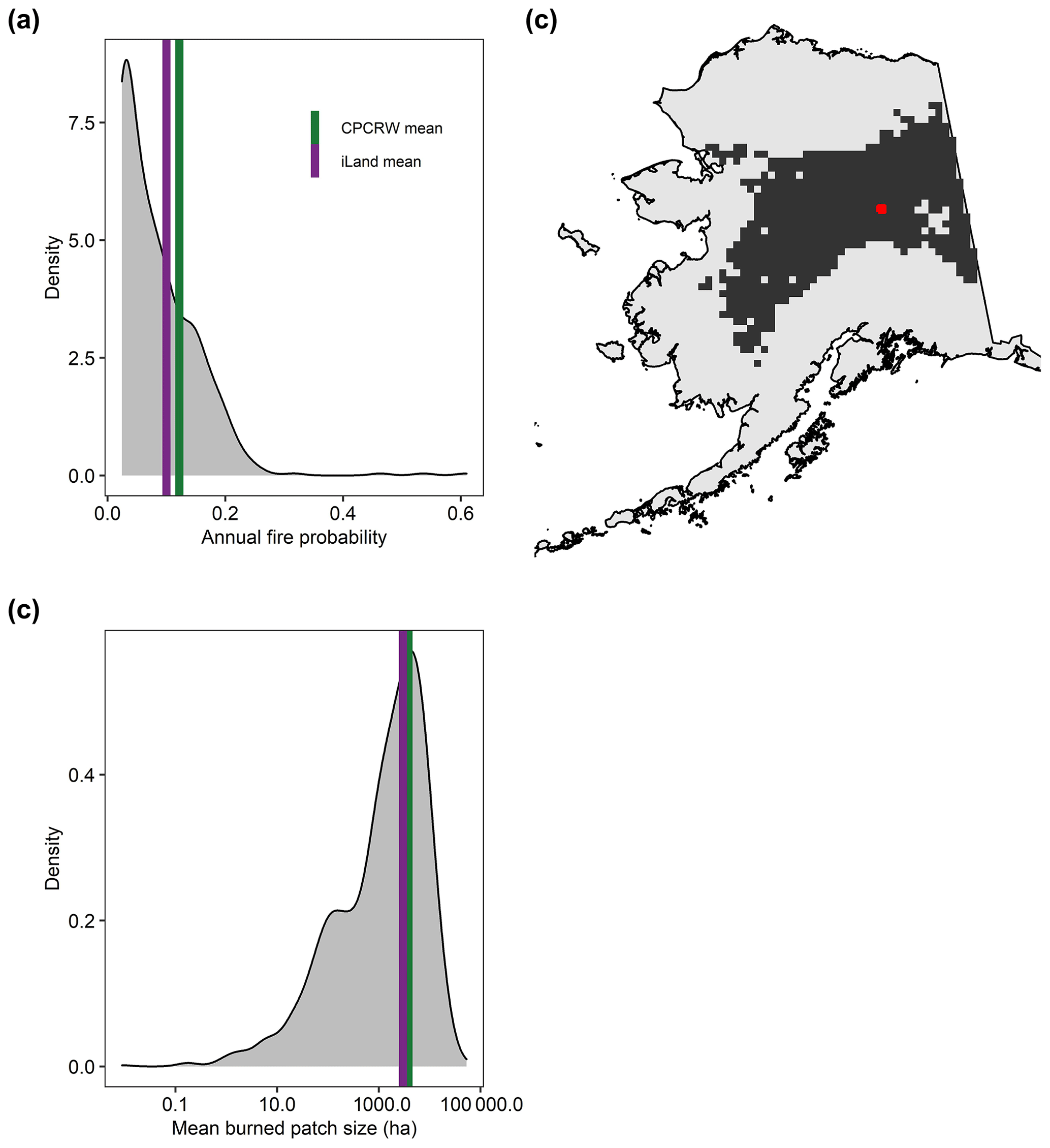
Figure 4Simulated and observed (a) annual fire probability and (b) mean burned patch size in a 61 000 ha landscape (Caribou Poker Creek Watershed, CPCRW) in interior Alaska. Model output is for years 201–300. Observations are from years 1980–2020. The gray density distribution shows observed values for all sampled 625 61 000 ha landscapes across the boreal domain of interior Alaska. (c) Map showing all 625 sampled landscapes as dark-gray squares. The red square shows the landscape simulated in iLand.
4.3 Landscape near-surface permafrost, moss, and SOL depth
The model simulated 39.3 % of forested area in the landscape as underlain by permafrost between years 261–300, compared to the estimated 33.4 % of forested area from the benchmarking product (Fig. 5a). Aspect was an important determinant of permafrost presence in the model and in observations (Fig. 5b). Simulated permafrost was overrepresented on north-facing slopes, as compared to the benchmarking product, but corresponded well in all other aspects. Near-surface permafrost presence also varied with dominant tree species in iLand. A total of 71 % percent of simulated black spruce forest area was underlain by near-surface permafrost, followed by 51 % of white spruce forest, 14 % of aspen-dominated stands, 11 % of mixed spruce, 6 % of mixed deciduous forest, and 0.2 % of birch-dominated forest.
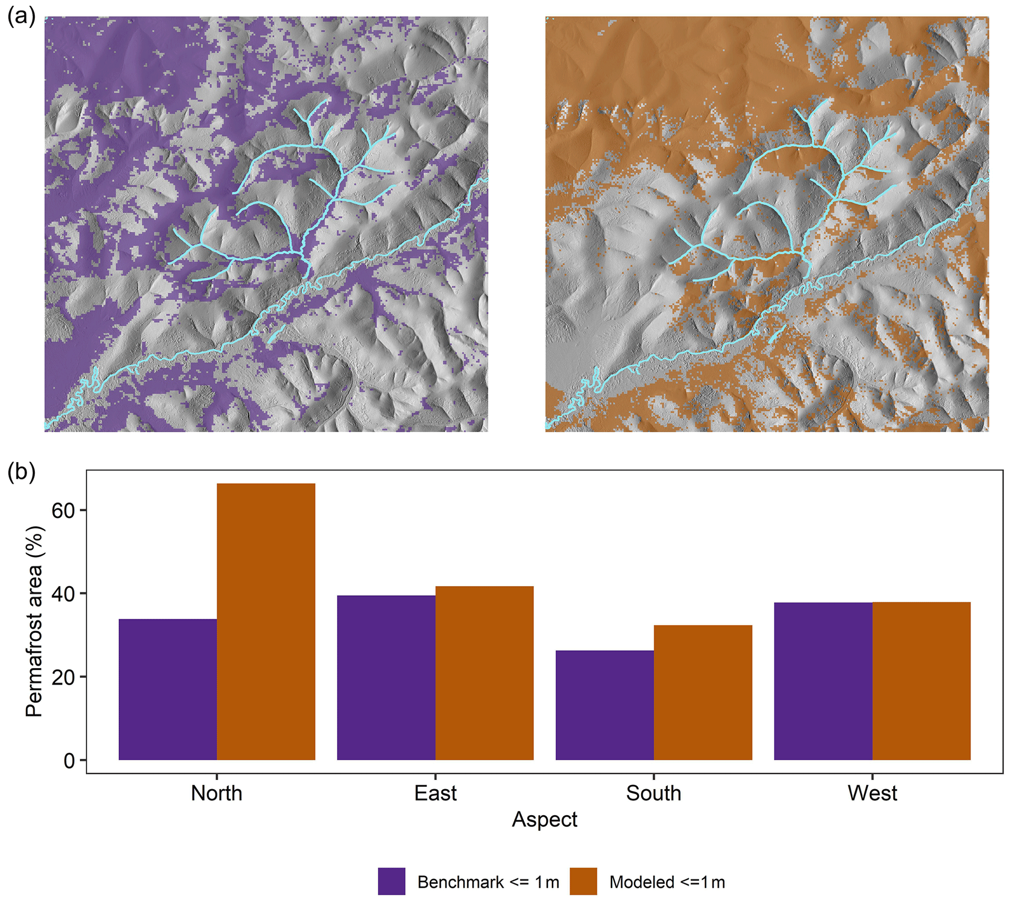
Figure 5(a) Observed and simulated near-surface (≤ 1 m deep) permafrost in a 61 000 ha forested landscape in interior Alaska. (b) Observed and simulated percent of forested area underlain by near-surface permafrost in the same landscape as a function of aspect. Simulated permafrost presence is for years 261–300 of the simulation. Benchmarking product is derived from years 1990–2013.
Soil-surface organic layer C in simulation year 300 averaged 4801 (2965–6575) g m−2. When broken out by dominant forest type, simulated SOL C closely corresponded to observations for all forest types where comparison was possible (Fig. 6a). Dead moss and litter depth across the landscape averaged 11.6 (7.4–15.5) cm in simulation year 300, and live moss depth averaged 5.4 (2.7–8.7) cm, with pronounced spatial heterogeneity (Fig. 6b). Tree species composition was an important determinant of total SOL depth (Fig. B2): the SOL was thickest in black-spruce-dominated stands, averaging 25 (21–27) cm, followed by white spruce: 17 (15–19) cm; mixed spruce: 14 (7–17) cm; aspen: 9 (4–11) cm; mixed deciduous: 5 (4–10) cm; and birch-dominated forest: 4 (3.7–4.1) cm. Fire occurrence also strongly influenced SOL depth. In black and white spruce stands, fire combusted 9 (6–12) cm on average. In contrast, almost no SOL was combusted in deciduous stands. The memory footprint of the permafrost and SOL module was approximately 15 MB (∼ 0.1 % of total memory footprint), and it increased overall runtime by 1 %.
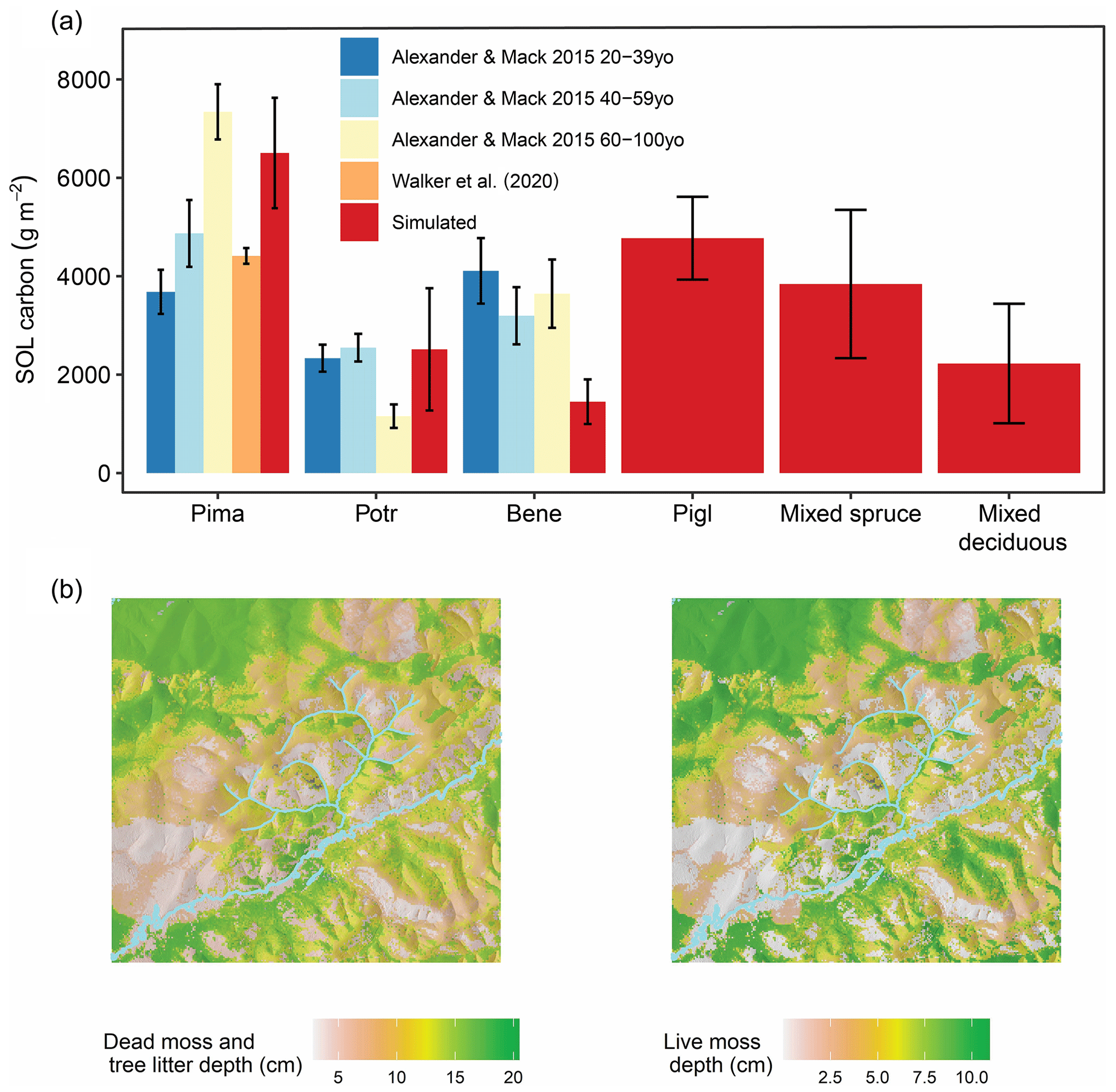
Figure 6(a) Observed and simulated surface organic layer carbon as a function of dominant forest type. Bars and whiskers show mean SOL carbon ±1 standard error due to limited availability of raw observational data. Simulated SOL carbon is from simulation year 300 in a 61 000 ha forested landscape in interior Alaska. Observations are from field sampling in other boreal forest stands. (b) Simulated dead moss and tree litter depth and live moss depth are from simulation year 300 in a 61 000 ha forested landscape in interior Alaska. Together, these two variables comprise the total surface organic layer in iLand.
4.4 Landscape-level tree species composition and forest structure
Between simulation year 0 and 300, forest cover increased from 48 811 to 60 629 ha, as trees colonized areas initialized as potential forest. The model was initialized with black spruce forest comprising 41 % of the land area, followed by white spruce (22 %), aspen (7 %), birch (6 %), and mixed forest (5 %) (Fig. 7a). By year 300, the land area dominated by black spruce remained high at 40 % (Fig. 7b). However, white-spruce-dominated forest area declined markedly to 2 % because black spruce trees colonized white spruce stands, as is commonly found in interior Alaska (Van Cleve and Viereck, 1981; Burns and Honkala, 1990). At the end of the simulation, mixed spruce stands comprised 42 % of land area. Aspen and birch also intermixed by year 300, with mixed deciduous forest covering 11 % of the landscape. The land area dominated by aspen in year 300 declined to 2 %, and birch-dominated forest declined to 3 % of the landscape. Rerunning simulations with the permafrost and SOL module turned off led to markedly different tree species composition compared to initial conditions and after 300 years of simulation where permafrost and SOL were dynamically represented (Fig. 8).
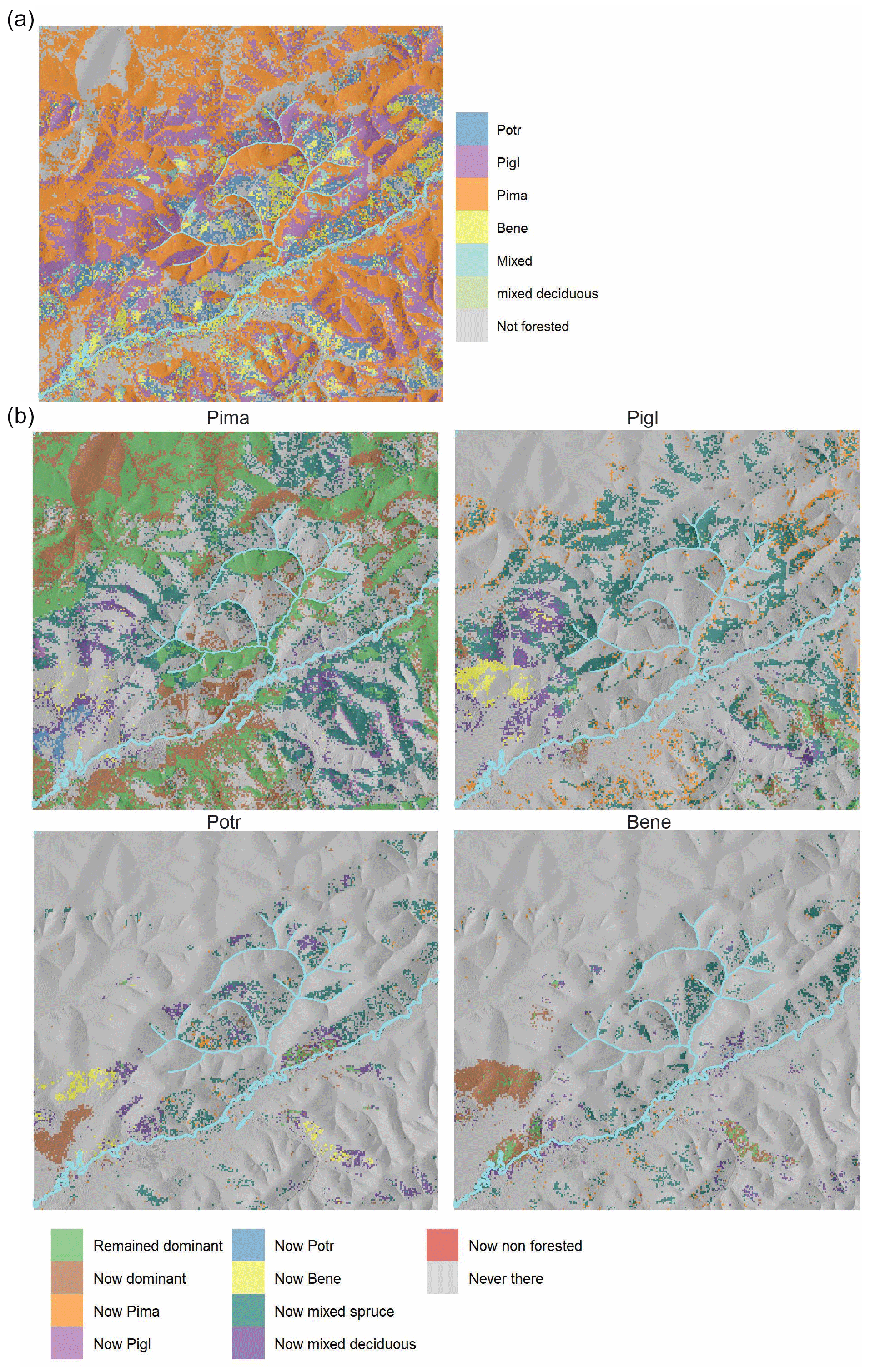
Figure 7(a) Tree species composition in a 61 000 ha forested landscape of interior Alaska used to initialize iLand. (b) Changes in tree species dominance over 300 years of simulation. Pima (Picea mariana): black spruce; Pigl (Picea glauca): white spruce; Potr (Populus tremuloides): trembling aspen; Bene (Betula neoalaskana): Alaskan birch.
Stand density and basal area in the model corresponded well with multiple field observation datasets in year 300 (Fig. 9). Aspen and birch stands were most dense, followed by black-spruce- and white-spruce-dominated stands. Deciduous-dominated stands also had the greatest basal area, followed by white spruce and black spruce stands (Fig. 9b).
Figure 8(a) Initial tree species composition, (b) tree species composition after 300 years when permafrost and SOL were simulated, and (c) tree species composition after 300 years when permafrost and SOL were not simulated in a 61 000 ha forested landscape of interior Alaska. Pima (Picea mariana): black spruce; Pigl (Picea glauca): white spruce; Potr (Populus tremuloides): trembling aspen; Bene (Betula neoalaskana): Alaskan birch. POLE-FM stands for Permafrost and Organic LayEr module for Forest Models.
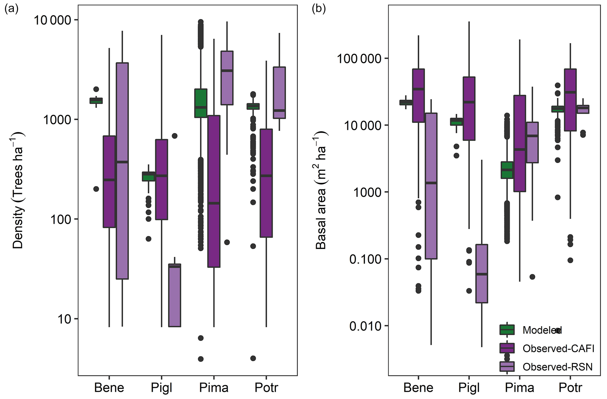
Figure 9Simulated and observed stand density and basal area broken out by dominant forest type in a 61 000 ha forested landscape of interior Alaska. Model output is from simulation year 300. Observations are from field sampling in other boreal forest stands (see main text for sources). Pima (Picea mariana): black spruce; Pigl (Picea glauca): white spruce; Potr (Populus tremuloides): trembling aspen; Bene (Betula neoalaskana): Alaskan birch.
Simulated aboveground live woody biomass across the landscape was within 28 % of the observed average. Aboveground live woody biomass in iLand was 51 931 (20 456–68 200) kg ha−1, on average, and observed biomass was 39 277 (9219–56 246) kg ha−1. Average simulated standing snag carbon differed from the observed average by 41 % (Fig. B3a). Simulated downed coarse-wood C varied markedly by dominant forest type and corresponded closely to field observations (Fig. B3b).
Simulated tree seedling density 2 years after fires closely matched field observations and varied with depth of postfire SOL (Fig. 10). Birch and aspen seedlings were most abundant where SOLs were shallow (0–5 cm), with 8.9 (6.1–13.1) and 6.2 (4.9–8.0) seedlings m−2 being established. Black spruce seedlings were the next most abundant, at 3.6 (0.3–4.8) seedlings m−2, followed by white spruce with 0.3 (0.2–0.4) seedlings m−2. Where SOLs were thicker (15–20 cm), black spruce density averaged 2.1 (1.3–3.1) seedlings m−2, and aspen, white spruce, and birch were rarely established.
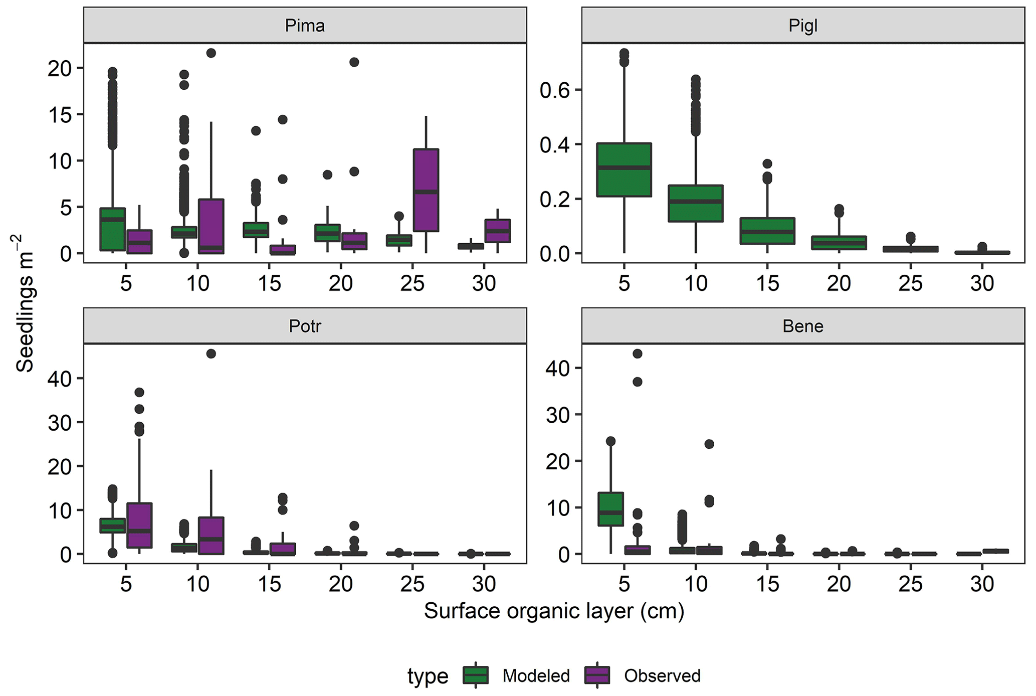
Figure 10Simulated and observed tree seedling density 2 years postfire as a function of surface organic layer depth. Model output is from recently burned areas in simulation years 261–300 in a 61 000 ha forested landscape in interior Alaska. Observations are from field sampling in other boreal forest stands (see main text for sources). Pima (Picea mariana: black spruce; Pigl (Picea glauca): white spruce; Potr (Populus tremuloides): trembling aspen; Bene (Betula neoalaskana): Alaskan birch.
Ecological legacies will determine how forests are affected by climate change and increasingly prevalent disturbances, like fire (Turetsky et al., 2016; Kannenberg et al., 2020; Hansen et al., 2022a). However, some legacies uniquely important to the structure and functioning of boreal forests (e.g., permafrost and SOLs) are rarely considered in models used to project 21st-century ecological change. Here, we present a new permafrost and SOL module that operates at fine temporal (daily) and spatial (1 ha) scales and is computationally efficient. The module simulates daily changes in active layer depth, moss production, and annual SOL accumulation (Fig. 1). When coupled to a forest model, it also represents the complex ecological effects of permafrost and SOLs on boreal forests and fire. With some exceptions discussed below, benchmarking results demonstrate that the model recreates temporal and spatial patterns consistent with observations at stand to landscape scales over days to centuries. Our model will contribute to improving 21st-century projections of boreal forest change.
Process-based simulation models are powerful tools for assessing how forests will change (Seidl, 2017; Albrich et al., 2020; Fisher and Koven, 2020). Forests often respond slowly to stressors relative to other ecological systems (Hughes et al., 2013; Turner et al., 2022). As a result, models must capture dynamic feedbacks among variables and represent the key legacies that accumulate over decades to centuries in order to project future trajectories of forests (Johnstone et al., 2016). Our objective was to mechanistically represent permafrost and SOLs and capture effects of daily variability in weather as well as the feedbacks that arise among forest dynamics, fires, and permafrost in topographically complex landscapes. The model was skilled at capturing inter-annual variability in maximum thaw depth, but it generally occurred later in simulations than in observations. There are a number of potential reasons for this. First, the model does not track the moisture content of the SOL separately from the mineral soil layer. In reality, the low bulk density of SOL relative to mineral soils leads to more variable moisture content and thus a greater range of thermal conductivities, which could lead to slower thawing in simulations if simulated SOL moisture was lower during the spring thaw (Fisher et al., 2016). Another potential explanation is that forest structure (density and leaf area index) and tree species composition have been shown to strongly modulate microclimate and permafrost thaw in complex ways (Stuenzi et al., 2021). Effects of forests on microclimate are also not yet included in the model. Finally, snow depth and melt play a critical role in active layer dynamics. Our model reasonably recreated snow accumulation patterns for most years but overestimated depth in years when snowpack was unusually deep. This is likely because iLand takes a relatively simple approach to simulating snow derived from Running and Coughlan (1988), which is not particularly mechanistic. For example, we used a single snow-density parameter value, which ignores compaction. In reality, snow density varies tremendously across landscapes and over time. In the future, our approach would benefit from separately tracking moisture content of the SOL and from a representation of forest structure and composition effects on microclimate. Further, a more advanced snow model could be added that includes key processes affecting snow depth and conductive properties, including the representation of variation in snow density, freeze–thaw cycles, and sublimation (Bormann et al., 2013; Jafarov et al., 2014).
At landscape scales, the model generally captured mosaics of near-surface permafrost, moss production, and SOL accumulation in a large forested area (∼ 61 000 ha of land area), but it did overestimate the area underlain by permafrost on north-facing slopes. This may have occurred for two reasons. First, the climate data used to force iLand were statistically downscaled to a 1 km resolution from a global general circulation model and thus do not perfectly capture variability in climate as a function of fine-scale variation in aspect and topography. Further downscaling using lapse rates might help improve simulations. Further, dominant forest type varies strongly with aspect in interior Alaska and in turn shapes SOL thickness and permafrost distributions. However, we lack landscape-level maps of individual tree species distributions to initialize the model. In the future, well-validated, remotely sensed tree species composition maps would markedly reduce initial condition uncertainty in forest simulations in interior Alaska (Hermosilla et al., 2022) and could improve landscape level simulations of permafrost distribution.
The module was designed to represent permafrost and SOL effects on forest dynamics and fire. In particular, it determines the water available to plants and accumulation of forest floor biomass, which serves as fuels for fire and influences postfire tree regeneration. When coupled with iLand, the model reproduced common secondary successional trajectories found in interior Alaska, including self-replacement and disturbance-induced abrupt transitions in forest types (Johnstone et al., 2010a, 2016). For example, when thick SOLs remained after fire in black spruce stands, self-replacement was common, leading to recovery of forests functionally and structurally similar to the prefire stands (Anderson et al., 2003; Johnstone and Kasischke, 2005). In contrast, when fires combusted most of the SOL in black spruce stands, abrupt transitions from spruce- to deciduous-dominated forest (mixtures of aspen and birch) occurred, consistent with regional trends documented in the last few decades (Johnstone et al., 2010a, 2020).
The boreal forest biome is warming at least 2 times faster than the global average (IPCC, 2021), causing climate-sensitive disturbances, like fire, to increase in frequency and severity (Seidl et al., 2020; Walker et al., 2020). Our permafrost and SOL module will help process-based modelers produce more accurate projections of how forests in the biome are likely to change over the next century. Better projections will resolve a number of important uncertainties, including (1) where increased burning due to climate change may reduce boreal fuel loads such that fire self-limitation emerges (Héon et al., 2014; Buma et al., 2022); (2) when shifts in postfire successional trajectories will initiate biophysical feedbacks that further alter regional climate; and (3) how climate change, fire, and permafrost thaw will interact to reshape boreal carbon cycling (Schurr et al., 2018; Schuur and Mack, 2018; Mack et al., 2021). Because boreal forests have disproportionate impacts on the climate system through biogeochemical and biophysical pathways, such information is essential to inform innovative and effective global climate mitigation and adaptation strategies.
A1 Carbon cycling in iLand
Carbon in live foliage, branch, stem, and root compartments and in standing snag, forest floor litter, downed coarse wood, and mineral soil organic material pools is dynamically modeled by iLand (Seidl et al., 2012b). Primary production is simulated with a radiation use efficiency approach. Carbon fixed by trees is then allocated to different tree compartments based on allometric equations, representing functional balance. Influxes of carbon from live compartments to dead-organic-matter pools are calculated based on leaf turnover rates, tree mortality, and snag dynamics. Snag fall occurs over time based on a species-specific half-life. When snags fall, they are added to the downed coarse-wood pool. Decomposition of dead-organic-matter pools is represented with a pool- and species-specific optimal decomposition rate (10 ∘C, no water limitation) that is then modified by prevailing temperature and precipitation.
A2 Forest fire in iLand
The model also includes robust representations of several natural disturbances, including forest fire (Seidl et al., 2014a, b; Hansen et al., 2020). Fire occurrence and spread are dynamically simulated at a 20 m resolution as a function of 20th-century fire probability and size distributions; landscape topography; model-generated wind speed and direction; and the proportion of total downed litter and coarse-wood pools that are burnable, which is determined by fuel moisture (as quantified by the Keetch–Byram drought index, KBDI). For every 20 m grid cell that burns, the available fuels are assumed combusted. Percent crown kill of live trees is estimated as a function of tree size, available fuel loads, and aridity. For the portion of live tree canopies that are killed, we assumed 90 % of foliage, 50 % of branch, and 30 % of the burned stem biomass are combusted. Tree mortality from fire is simulated probabilistically based on tree size; percent crown kill; and bark thickness, a model parameter that varies by tree species. If a tree dies, the non-combusted foliage and branches are added to the downed litter and coarse-wood pools. Portions of killed tree stems that were not combusted enter the standing snag pool.
Table B1Species parameters for interior Alaskan boreal forest. Pima: Picea mariana (black spruce); Pigl: Picea glauca (white spruce); Potr: Populus tremuloides (trembling aspen); Bene: Betula neoalaskana (Alaskan birch); dim: dimensionless; exp: expression; sdlings: seedlings. See Hansen et al. (2021) for sources.
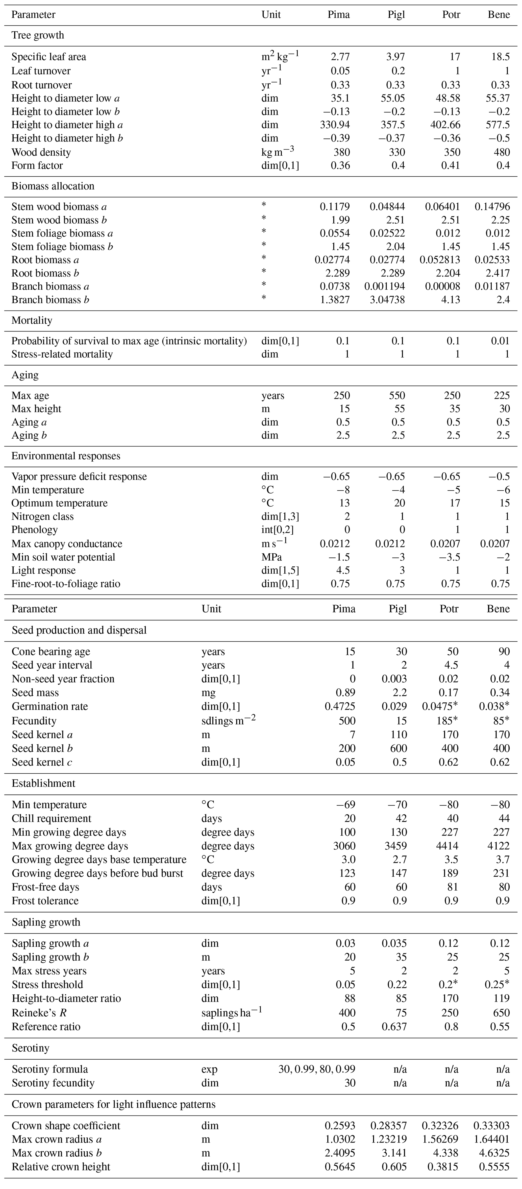
* Adjusted from Hansen et al. (2021) with addition of permafrost module. n/a – not applicable
Table B2Carbon cycle parameters of iLand. Pima: Picea mariana (black spruce); Pigl: Picea glauca (white spruce); Potr: Populus tremuloides (trembling aspen); Bene: Betula neoalaskana (Alaskan birch).
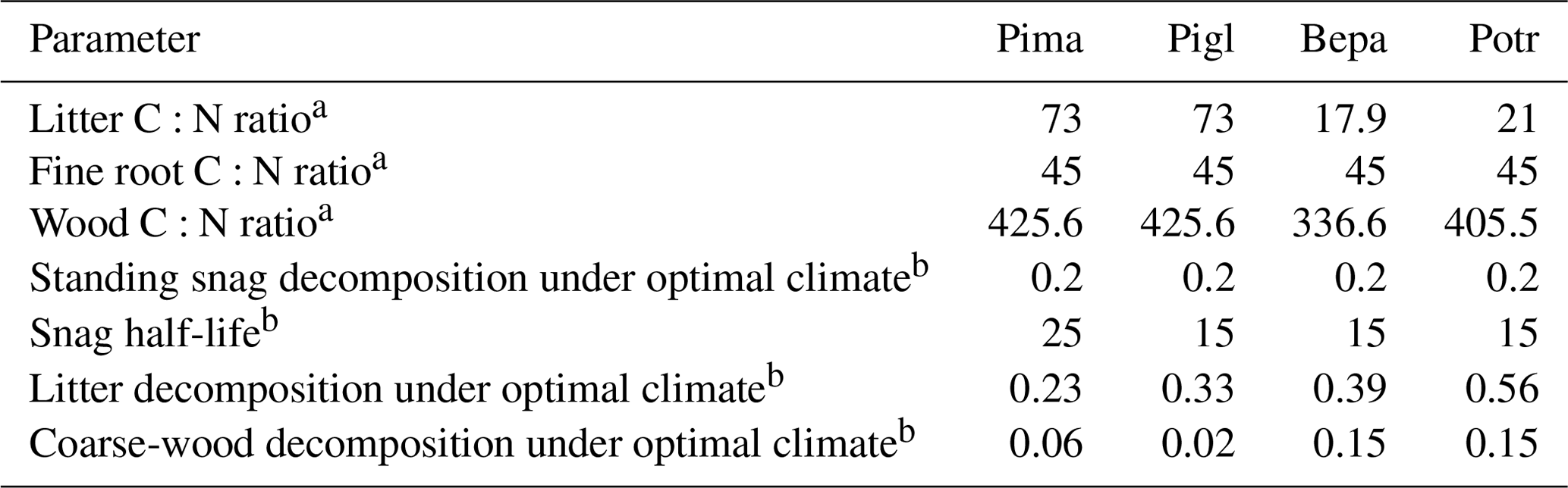
a Alexander and Mack (2015). b This study.
Table B3Rules for converting plant functional type maps from Wang et al. (2020) to species-level maps for initializing iLand.
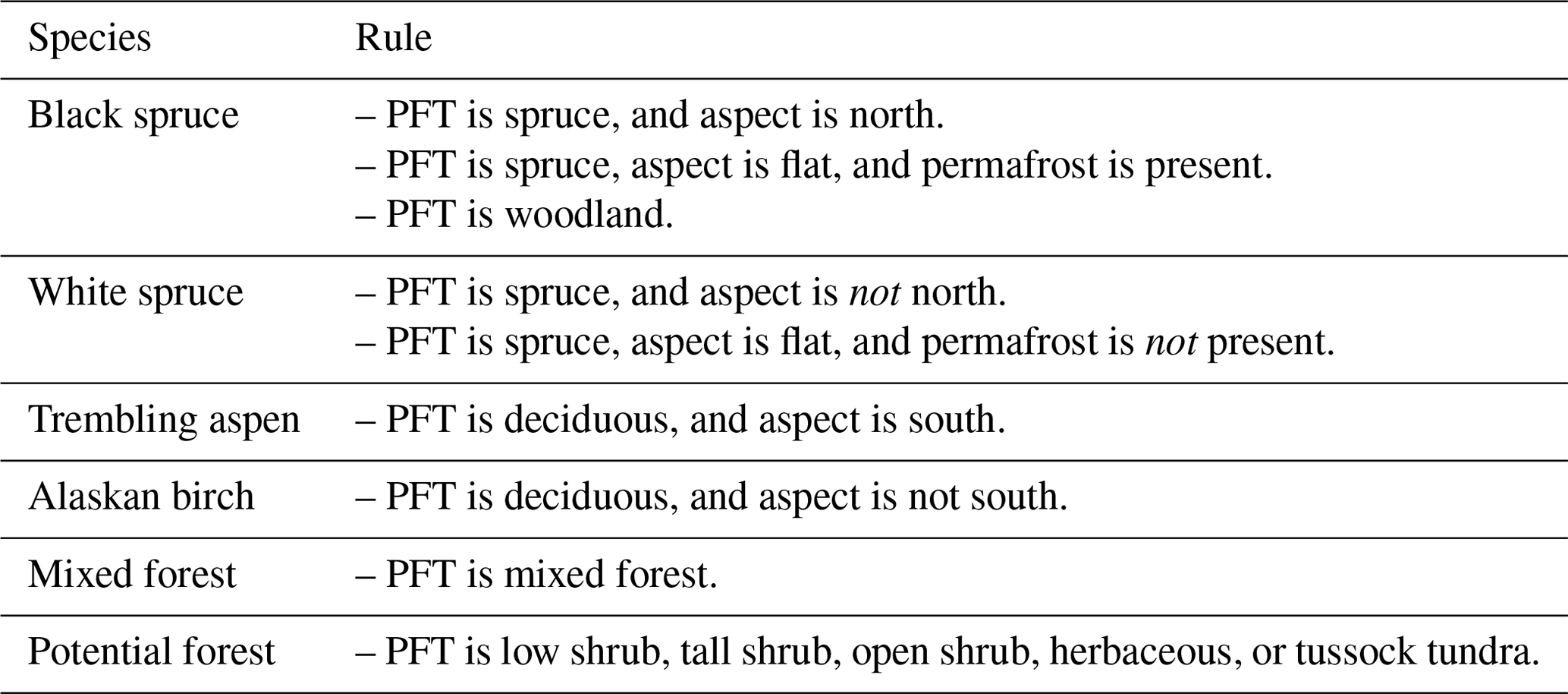
Table B4Initial conditions for iLand carbon cycle. Pima: Picea mariana (black spruce); Pigl: Picea glauca (white spruce); Potr: Populus tremuloides (trembling aspen); Bene: Betula neoalaskana (Alaskan birch).
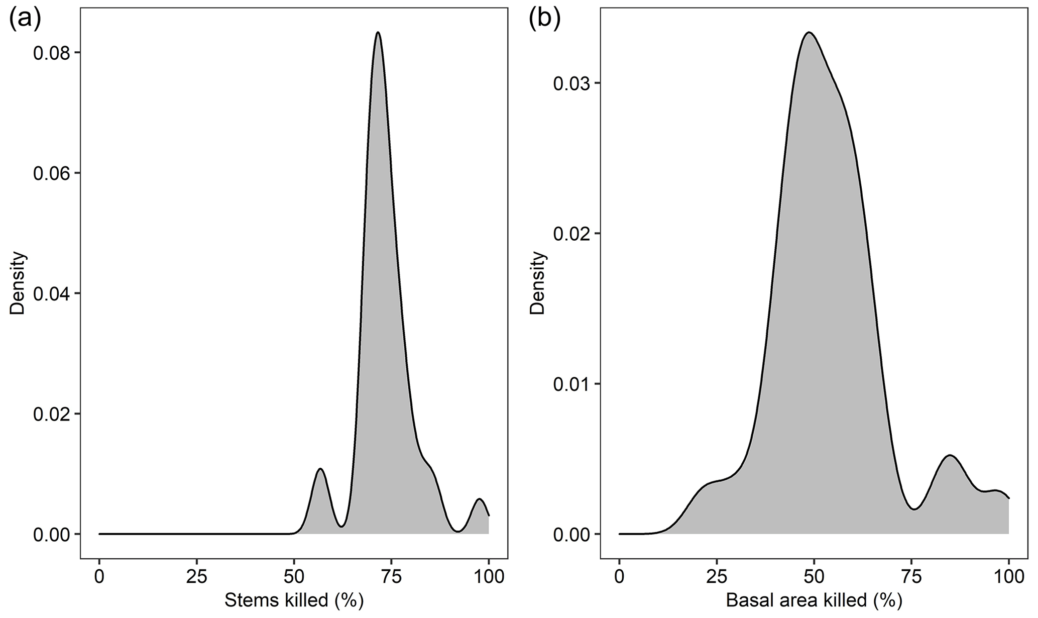
Figure B1Simulated percent of (a) stems killed and (b) basal area killed by fire in a 61 000 ha forested landscape in interior Alaska. Model output is from simulation years 201–300.
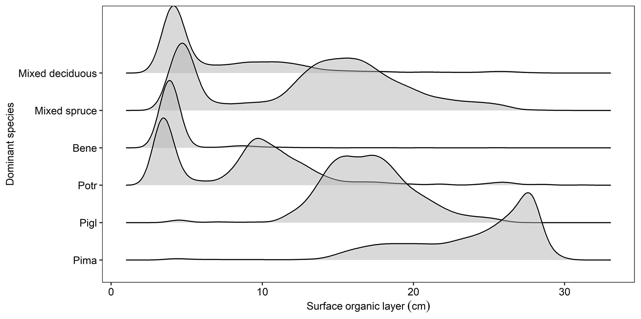
Figure B2Simulated surface organic layer depth as a function of dominant forest type in a 61 000 ha forested landscape in interior Alaska. Model output is from simulation year 300.
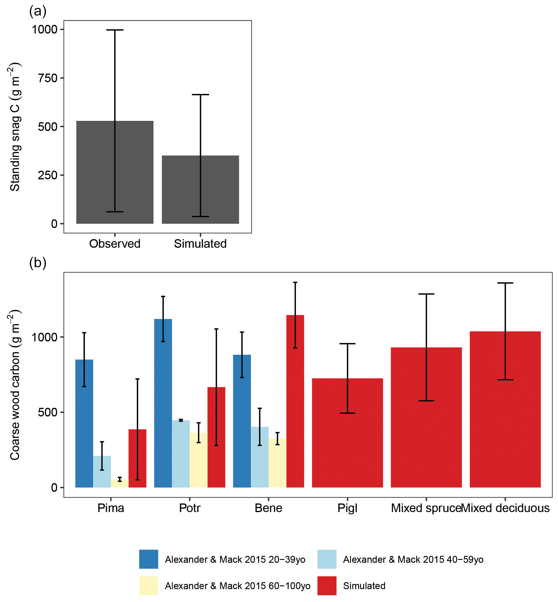
Figure B3Observed and simulated (a) standing snag carbon and (b) downed coarse-wood carbon as a function of dominant forest type. Bars and whiskers show means ±1 standard deviation in plot (a) and means ±1 standard error due to the limited availability of the raw field observations. Modeled carbon stocks are from simulation year 300 in a 61 000 ha forested landscape in interior Alaska. Observations are from field sampling in other boreal forest stands.
The source code is available as a Supplement to this paper. The model executable and source code, project directories, and analysis R scripts used in this project are also available at the Cary Institute of Ecosystem Studies data repository (DOI: https://doi.org/10.25390/caryinstitute.21339090; Hansen et al., 2022). A technical description of the permafrost and SOL module is available at https://iland-model.org/permafrost (last access: 1 October 2022).
The supplement related to this article is available online at: https://doi.org/10.5194/gmd-16-2011-2023-supplement.
WR and WDH developed the permafrost and SOL module, and WDH conducted benchmarking simulations, analyzed outputs, and wrote the paper. All co-authors contributed to the paper.
The contact author has declared that none of the authors has any competing interests.
Publisher's note: Copernicus Publications remains neutral with regard to jurisdictional claims in published maps and institutional affiliations.
We are grateful to Brendan Rogers, Scott Goetz, Michelle Mack, and Xanthe Walker, who provided feedback on an earlier draft of this paper. Winslow D. Hansen acknowledges support from the National Science Foundation (grant no. OPP 2116863) and the Royal Bank of Canada. Rupert Seidl and Werner Rammer acknowledge funding from the European Research Council under the European Union's Horizon 2020 research and innovation program (grant agreement 101001905). Benjamin Gaglioti acknowledges support from the Joint Fire Sciences Program (project 20-2-01-13).
This research has been supported by the National Science Foundation (grant no. OPP 2116863), the European Research Council under the European Union’s Horizon 2020 research and innovation program (grant agreement 101001905), the Joint Fire Sciences Program (project 20-2-01-13), and the Royal Bank of Canada.
This paper was edited by Marko Scholze and reviewed by Simone Maria Stuenzi and one anonymous referee.
Abbott, B. W. and Jones, J. B.: Permafrost collapse alters soil carbon stocks, respiration, CH4, and N2O in upland tundra, Glob.Change Biol., 21, 4570–4587, https://doi.org/10.1111/gcb.13069, 2015.
Albrich, K., Rammer, W., Turner, M. G., Ratajczak, Z., Braziunas, K. H., Hansen, W. D., and Seidl, R.: Simulating forest resilience: A review, Global Ecol. Biogeogr., 29, 2082–2096, https://doi.org/10.1111/geb.13197, 2020.
Alexander, H. D. and Mack, M. C.: A canopy shift in interior Alaskan boreal forests: Consequences for above- and belowground carbon and nitrogen pools during post-fire succession, Ecosystems, 19, 98–114, https://doi.org/10.1007/s10021-015-9920-7, 2016.
Anderegg, W. R. L., Wu, C., Acil, N., Carvalhais, N., Pugh, T. A. M., Sadler, J. P., and Seidl, R.: A climate risk analysis of Earth's forests in the 21st century, Science, 377, 1099–1103, https://doi.org/10.1126/science.abp9723, 2022.
Anderson, P. M., Edwards, M. E., and Brubaker, L. B.: Results and paleoclimate implications of 35 years of paleoecological research in Alaska, in: Developments in Quaternary Sciences, vol. 1, Elsevier, 427–440, https://doi.org/10.1016/S1571-0866(03)01019-4, 2003.
Baltzer, J. L., Veness, T., Chasmer, L. E., Sniderhan, A. E., and Quinton, W. L.: Forests on thawing permafrost: fragmentation, edge effects, and net forest loss, Glob. Change Biol., 20, 824–834, https://doi.org/10.1111/gcb.12349, 2014.
Baltzer, J. L., Day, N. J., Walker, X. J., Greene, D., Mack, M. C., Alexander, H. D., Arseneault, D., Barnes, J., Bergeron, Y., Boucher, Y., Bourgeau-Chavez, L., Brown, C. D., Carrière, S., Howard, B. K., Gauthier, S., Parisien, M.-A., Reid, K. A., Rogers, B. M., Roland, C., Sirois, L., Stehn, S., Thompson, D. K., Turetsky, M. R., Veraverbeke, S., Whitman, E., Yang, J., and Johnstone, J. F.: Increasing fire and the decline of fire adapted black spruce in the boreal forest, P. Natl. Acad. Sci. USA, 118, e2024872118, https://doi.org/10.1073/pnas.2024872118, 2021.
Beer, C., Lucht, W., Gerten, D., Thonicke, K., and Schmullius, C.: Effects of soil freezing and thawing on vegetation carbon density in Siberia: A modeling analysis with the Lund-Potsdam-Jena Dynamic Global Vegetation Model (LPJ-DGVM), Global Biogeochem. Cy., 21, GB1012, https://doi.org/10.1029/2006GB002760, 2007.
Bennett, K. E., Cherry, J. E., Balk, B., and Lindsey, S.: Using MODIS estimates of fractional snow cover area to improve streamflow forecasts in interior Alaska, Hydrol. Earth Syst. Sci., 23, 2439–2459, https://doi.org/10.5194/hess-23-2439-2019, 2019.
Bonan, G.: Surface Energy Fluxes, in: Climate Change and Terrestrial Ecosystem Modeling, University of Cambridge Press, Cambridge, UK, 101–114, https://doi.org/10.1017/9781107339217, 2019.
Bonan, G. B.: A biophysical surface energy budget analysis of soil temperature in the boreal forests of interior Alaska, Water Resour. Res., 27, 767–781, https://doi.org/10.1029/91WR00143, 1991.
Bonan, G. B. and Korzuhin, M. D.: Simulation of moss and tree dynamics in the boreal forests of interior Alaska, Vegetatio, 84, 31–44, https://doi.org/10.1007/BF00054663, 1989.
Bormann, K. J., Westra, S., Evans, J. P., and McCabe, M. F.: Spatial and temporal variability in seasonal snow density, J. Hydrol., 484, 63–73, https://doi.org/10.1016/j.jhydrol.2013.01.032, 2013.
Brown, C. D. and Johnstone, J. F.: Once burned, twice shy: Repeat fires reduce seed availability and alter substrate constraints on Picea mariana regeneration, Forest Ecol. Manage., 266, 34–41, https://doi.org/10.1016/j.foreco.2011.11.006, 2012.
Brown, D. R. N., Jorgenson, M. T., Kielland, K., Verbyla, D. L., Prakash, A., and Koch, J. C.: Landscape effects of wildfire on permafrost distribution in interior Alaska derived from remote sensing, Remote Sensing, 8, 654, https://doi.org/10.3390/rs8080654, 2016.
Buma, B., Hayes, K., Weiss, S., and Lucash, M.: Short-interval fires increasing in the Alaskan boreal forest as fire self-regulation decays across forest types, Sci. Rep., 12, 4901, https://doi.org/10.1038/s41598-022-08912-8, 2022.
Burns, R. M. and Honkala, B. H.: Silvics Manual Volume 1-Conifers and Volume 2-Hardwoods, 2nd Edn., U.S. Department of Agriculture, Forest Service, Washington DC, US Library of Congress catalog number: 86-60058, 1990.
Chapin, F. S., Randerson, J. T., McGuire, A. D., Foley, J. A., and Field, C. B.: Changing feedbacks in the climate–biosphere system, Front. Ecol. Environ., 6, 313–320, https://doi.org/10.1890/080005, 2008.
Chylek, P., Folland, C., Klett, J. D., Wang, M., Hengartner, N., Lesins, G., and Dubey, M. K.: Annual Mean Arctic Amplification 1970–2020: Observed and Simulated by CMIP6 Climate Models, Geophys. Res. Lett., 49, e2022GL099371, https://doi.org/10.1029/2022GL099371, 2022.
Cook, B. I., Bonan, G. B., Levis, S., and Epstein, H. E.: The thermoinsulation effect of snow cover within a climate model, Clim. Dynam., 31, 107–124, https://doi.org/10.1007/s00382-007-0341-y, 2008.
Dearborn, K. D. and Baltzer, J. L.: Unexpected greening in a boreal permafrost peatland undergoing forest loss is partially attributable to tree species turnover, Glob. Change Biol., 27, 2867–2882, https://doi.org/10.1111/gcb.15608, 2021.
Farouki, O. T.: The thermal properties of soils in cold regions, Cold Reg. Sci. Technol., 5, 67–75, https://doi.org/10.1016/0165-232X(81)90041-0, 1981.
Fisher, J. P., Estop-Aragonés, C., Thierry, A., Charman, D. J., Wolfe, S. A., Hartley, I. P., Murton, J. B., Williams, M., and Phoenix, G. K.: The influence of vegetation and soil characteristics on active-layer thickness of permafrost soils in boreal forest, Glob. Change Biol., 22, 3127–3140, https://doi.org/10.1111/gcb.13248, 2016.
Fisher, R. A. and Koven, C. D.: Perspectives on the future of land surface models and the challenges of representing complex terrestrial systems, J. Adv. Model. Earth Sy., 12, e2018MS001453, https://doi.org/10.1029/2018ms001453, 2020.
Foley, J. A., Kutzbach, J. E., Coe, M. T., and Levis, S.: Feedbacks between climate and boreal forests during the Holocene epoch, Nature, 371, 52–54, https://doi.org/10.1038/371052a0, 1994.
Foster, A. C., Armstrong, A. H., Shuman, J. K., Shugart, H. H., Rogers, B. M., Mack, M. C., Goetz, S. J., and Ranson, K. J.: Importance of tree- and species-level interactions with wildfire, climate, and soils in interior Alaska: Implications for forest change under a warming climate, Ecol. Model., 409, 108765, https://doi.org/10.1016/j.ecolmodel.2019.108765, 2019.
Foster, A. C., Shuman, J. K., Rogers, B. M., Walker, X. J., Mack, M. C., Bourgeau-Chavez, L. L., Veraverbeke, S., and Goetz, S. J.: Bottom-up drivers of future fire regimes in western boreal North America, Environ. Res. Lett., 17, 025006, https://doi.org/10.1088/1748-9326/ac4c1e, 2022.
Gent, P. R., Danabasoglu, G., Donner, L. J., Holland, M. M., Hunke, E. C., Jayne, S. R., Lawrence, D. M., Neale, R. B., Rasch, P. J., Vertenstein, M., Worley, P. H., Yang, Z.-L., and Zhang, M.: The Community Climate System Model Version 4, J. Climate, 24, 4973–4991, https://doi.org/10.1175/2011JCLI4083.1, 2011.
Gibson, C. M., Chasmer, L. E., Thompson, D. K., Quinton, W. L., Flannigan, M. D., and Olefeldt, D.: Wildfire as a major driver of recent permafrost thaw in boreal peatlands, Nat. Commun., 9, 3041, https://doi.org/10.1038/s41467-018-05457-1, 2018.
Grimm, V., Revilla, E., Berger, U., Jeltsch, F., Mooij, W. M., Railsback, S. F., Thulke, H.-H., Weiner, J., Wiegand, T., and DeAngelis, D. L.: Pattern-oriented modeling of agent-based complex systems: Lessons from ecology, Science, 310, 987–991, https://doi.org/10.1126/science.1116681, 2005.
Gustafson, E. J., Miranda, B. R., Shvidenko, A. Z., and Sturtevant, B. R.: Simulating growth and competition on wet and waterlogged soils in a forest landscape model, Front. Ecol. Evol., 8, 598775, https://doi.org/10.3389/fevo.2020.598775, 2020.
Hansen, W. D., Braziunas, K. H., Rammer, W., Seidl, R., and Turner, M. G.: It takes a few to tango: Changing climate and fire regimes can cause regeneration failure of two subalpine conifers, Ecology, 99, 966–977, https://doi.org/10.1002/ecy.2181, 2018.
Hansen, W. D., Abendroth, D., Rammer, W., Seidl, R., and Turner, M.: Can wildland fire management alter 21st-century subalpine fire and forests in Grand Teton National Park, Wyoming, USA?, Ecol. Appl., 30, e02030, https://doi.org/10.1002/eap.2030, 2020.
Hansen, W. D., Fitzsimmons, R., Olnes, J., and Williams, A. P.: An alternate vegetation type proves resilient and persists for decades following forest conversion in the North American boreal biome, J. Ecol., 109, 85–98, https://doi.org/10.1111/1365-2745.13446, 2021.
Hansen, W. D., Schwartz, N. B., Williams, A. P., Albrich, K., Kueppers, L. M., Rammig, A., Reyer, C. P. O., Staver, A. C., and Seidl, R.: Global forests are influenced by legacies of past inter-annual temperature variability, Environ. Res. Ecol., 1, 011001, https://doi.org/10.1088/2752-664X/ac6e4a, 2022a.
Hansen, W. D., Foster, A., Gaglioti, B., Seidl, R., and Rammer, W.: Data and code associated with: The Permafrost and Organic LayEr module for Forest Models (POLE-FM) 1.0, Cary Institute [code and data set], https://doi.org/10.25390/caryinstitute.21339090.v3, 2022b.
Hengl, T., Jesus, J. M. de, Heuvelink, G. B. M., Gonzalez, M. R., Kilibarda, M., Blagotić, A., Shangguan, W., Wright, M. N., Geng, X., Bauer-Marschallinger, B., Guevara, M. A., Vargas, R., MacMillan, R. A., Batjes, N. H., Leenaars, J. G. B., Ribeiro, E., Wheeler, I., Mantel, S., and Kempen, B.: SoilGrids250m: Global gridded soil information based on machine learning, PLOS ONE, 12, e0169748, https://doi.org/10.1371/journal.pone.0169748, 2017.
Héon, J., Arseneault, D., and Parisien, M.-A.: Resistance of the boreal forest to high burn rates, P. Natl. Acad. Sci. USA, 111, 13888–13893, https://doi.org/10.1073/pnas.1409316111, 2014.
Hermosilla, T., Bastyr, A., Coops, N. C., White, J. C., and Wulder, M. A.: Mapping the presence and distribution of tree species in Canada's forested ecosystems, Remote Sens. Environ., 282, 113276, https://doi.org/10.1016/j.rse.2022.113276, 2022.
Hijmans, R. J.: Spatial Data analysis, Rpackage version 1.7-22 [software], https://rspatial.org/ (last access: 1 March 2022), 2021.
Hinzman, L. D., Kane, D. L., Gieck, R. E., and Everett, K. R.: Hydrologic and thermal properties of the active layer in the Alaskan Arctic, Cold Reg. Sci. Technol., 19, 95–110, https://doi.org/10.1016/0165-232X(91)90001-W, 1991.
Hughes, T. P., Linares, C., Dakos, V., van de Leemput, I. A., and van Nes, E. H.: Living dangerously on borrowed time during slow, unrecognized regime shifts, Trends Ecol. Evol., 28, 149–55, https://doi.org/10.1016/j.tree.2012.08.022, 2013.
IPCC: Climate Change 2021: The Physical Science Basis. Contribution of Working Group I to the Sixth Assessment Report of the Intergovernmental Panel on Climate Change, Cambridge University Press, https://doi.org/10.1017/9781009157896, 2021.
Jafarov, E. E., Nicolsky, D. J., Romanovsky, V. E., Walsh, J. E., Panda, S. K., and Serreze, M. C.: The effect of snow: How to better model ground surface temperatures, Cold Reg. Sci. Technol., 102, 63–77, https://doi.org/10.1016/j.coldregions.2014.02.007, 2014.
Jean, M., Melvin, A. M., Mack, M. C., and Johnstone, J. F.: Broadleaf litter controls feather moss growth in black spruce and birch forests of interior Alaska, Ecosystems, 23, 18–33, https://doi.org/10.1007/s10021-019-00384-8, 2020.
Johnstone, J. and Chapin, F.: Effects of soil burn severity on post-fire tree recruitment in boreal forest, Ecosystems, 9, 14–31, https://doi.org/10.1007/s10021-004-0042-x, 2006.
Johnstone, J., Boby, L., Tissier, E., Mack, M., Verbyla, D., and Walker, X.: Postfire seed rain of black spruce, a semiserotinous conifer, in forests of interior Alaska, Can. J. Forest Res., 39, 1575–1588, https://doi.org/10.1139/X09-068, 2009.
Johnstone, J. F. and Kasischke, E. S.: Stand-level effects of soil burn severity on postfire regeneration in a recently burned black spruce forest, Can. J. Forest Res., 35, 2151–2163, 2005.
Johnstone, J. F., Hollingsworth, T. N., Chapin, F. S., and Mack, M. C.: Changes in fire regime break the legacy lock on successional trajectories in Alaskan boreal forest, Glob. Change Biol., 16, 1281–1295, https://doi.org/10.1111/j.1365-2486.2009.02051.x, 2010a.
Johnstone, J. F., Chapin, F. S., Hollingsworth, T. N., Mack, M. C., Romanovsky, V., and Turetsky, M.: Fire, climate change, and forest resilience in interior Alaska, Can. J. Forest Res., 40, 1302–1312, https://doi.org/10.1139/X10-061, 2010b.
Johnstone, J. F., Allen, C. D., Franklin, J. F., Frelich, L. E., Harvey, B. J., Higuera, P. E., Mack, M. C., Meentemeyer, R. K., Metz, M. R., Perry, G. L., Schoennagel, T., and Turner, M. G.: Changing disturbance regimes, ecological memory, and forest resilience, Front. Ecol. Environ., 14, 369–378, https://doi.org/10.1002/fee.1311, 2016.
Johnstone, J. F., Celis, G., Chapin, F. S., Hollingsworth, T. N., Jean, M., and Mack, M. C.: Factors shaping alternate successional trajectories in burned black spruce forests of Alaska, Ecosphere, 11, e03129, https://doi.org/10.1002/ecs2.3129, 2020.
Jorgenson, M. T., Romanovsky, V., Harden, J., Shur, Y., O'Donnell, J., Schuur, E. A. G., Kanevskiy, M., and Marchenko, S.: Resilience and vulnerability of permafrost to climate change, Can. J. Forest Res., 40, 1219–1236, https://doi.org/10.1139/X10-060, 2010.
Kannenberg, S. A., Schwalm, C. R., and Anderegg, W. R. L.: Ghosts of the past: how drought legacy effects shape forest functioning and carbon cycling, Ecol. Lett., 23, 891–901, https://doi.org/10.1111/ele.13485, 2020.
Karra, S., Painter, S. L., and Lichtner, P. C.: Three-phase numerical model for subsurface hydrology in permafrost-affected regions (PFLOTRAN-ICE v1.0), The Cryosphere, 8, 1935–1950, https://doi.org/10.5194/tc-8-1935-2014, 2014.
Kasischke, E. S. and Johnstone, J. F.: Variation in postfire organic layer thickness in a black spruce forest complex in interior Alaska and its effects on soil temperature and moisture, Can. J. Forest Res., 35, 2164–2177, https://doi.org/10.1139/x05-159, 2005.
Kruse, S., Stuenzi, S. M., Boike, J., Langer, M., Gloy, J., and Herzschuh, U.: Novel coupled permafrost–forest model (LAVESI–CryoGrid v1.0) revealing the interplay between permafrost, vegetation, and climate across eastern Siberia, Geosci. Model Dev., 15, 2395–2422, https://doi.org/10.5194/gmd-15-2395-2022, 2022.
Lorenz, K. and Lal, R.: Carbon Dynamics and Pools in Major Forest Biomes of the World, in: Carbon Sequestration in Forest Ecosystems, edited by: Lorenz, K. and Lal, R., Springer Netherlands, Dordrecht, 159–205, https://doi.org/10.1007/978-90-481-3266-9_4, 2010.
Mack, M. C., Walker, X. J., Johnstone, J. F., Alexander, H. D., Melvin, A. M., Jean, M., and Miller, S. N.: Carbon loss from boreal forest wildfires offset by increased dominance of deciduous trees, Science, 372, 280–283, https://doi.org/10.1126/science.abf3903, 2021.
Malone, T., Liang, J., and Packee, E. C.: Cooperative Alaska Forest Inventory, United States Department of Agriculture, Forest Service, Pacific Northwester Research Station, https://doi.org/10.2737/PNW-GTR-785, 2009.
Mekonnen, Z. A., Riley, W. J., Randerson, J. T., Grant, R. F., and Rogers, B. M.: Expansion of high-latitude deciduous forests driven by interactions between climate warming and fire, Nature Plants, 5, 952–958, https://doi.org/10.1038/s41477-019-0495-8, 2019.
Melvin, A. M., Mack, M. C., Johnstone, J. F., Mcguire, A. D., Genet, H., and Schuur, E. A. G.: Differences in ecosystem carbon distribution and nutrient cycling linked to forest tree species composition in a mid-successional boreal forest, Ecosystems, 18, 1472–1488, https://doi.org/10.1007/s10021-015-9912-7, 2015.
Obu, J., Westermann, S., Bartsch, A., Berdnikov, N., Christiansen, H. H., Dashtseren, A., Delaloye, R., Elberling, B., Etzelmüller, B., Kholodov, A., Khomutov, A., Kääb, A., Leibman, M. O., Lewkowicz, A. G., Panda, S. K., Romanovsky, V., Way, R. G., Westergaard-Nielsen, A., Wu, T., Yamkhin, J., and Zou, D.: Northern Hemisphere permafrost map based on TTOP modelling for 2000–2016 at 1 km2 scale, Earth-Sci. Rev., 193, 299–316, https://doi.org/10.1016/j.earscirev.2019.04.023, 2019.
O'Donnell, J. A., Romanovsky, V. E., Harden, J. W., and McGuire, A. D.: The effect of moisture content on the thermal conductivity of moss and organic soil horizons from black spruce ecosystems in interior Alaska, Soil Sci., 174, 646–651, https://doi.org/10.1097/SS.0b013e3181c4a7f8, 2009.
Ogle, K., Barber, J. J., Barron-Gafford, G. A., Bentley, L. P., Young, J. M., Huxman, T. E., Loik, M. E., and Tissue, D. T.: Quantifying ecological memory in plant and ecosystem processes, Ecol. Lett., 18, 221–235, https://doi.org/10.1111/ele.12399, 2015.
Pastick, N. J., Jorgenson, M. T., Wylie, B. K., Nield, S. J., Johnson, K. D., and Finley, A. O.: Distribution of near-surface permafrost in Alaska: Estimates of present and future conditions, Remote Sens. Environ., 168, 301–315, https://doi.org/10.1016/j.rse.2015.07.019, 2015.
Perreault, J., Fortier, R., and Molson, J. W.: Numerical modelling of permafrost dynamics under climate change and evolving ground surface conditions: application to an instrumented permafrost mound at Umiujaq, Nunavik (Québec), Canada, Écoscience, 28, 377–397, https://doi.org/10.1080/11956860.2021.1949819, 2021.
Phillips, C. A., Rogers, B. M., Elder, M., Cooperdock, S., Moubarak, M., Randerson, J. T., and Frumhoff, P. C.: Escalating carbon emissions from North American boreal forest wildfires and the climate mitigation potential of fire management, Sci. Adv., 8, eabl7161, https://doi.org/10.1126/sciadv.abl7161, 2022.
Potter, S., Solvik, K., Erb, A., Goetz, S. J., Johnstone, J. F., Mack, M. C., Randerson, J. T., Román, M. O., Schaaf, C. L., Turetsky, M. R., Veraverbeke, S., Walker, X. J., Wang, Z., Massey, R., and Rogers, B. M.: Climate change decreases the cooling effect from postfire albedo in boreal North America, Glob. Change Biol., 26, 1592–1607, https://doi.org/10.1111/gcb.14888, 2020.
R Core Team: R: A Language and Environment for Statistical Computing, R Foundation for Statistical Computing, Vienna, Austria, [software], https://www.R-project.org/ (last access: 1 March 2022), 2021.
Riseborough, D. W.: Exploring the Parameters of a Simple Model of the Permafrost – Climate Relationship, Carleton University, Ottawa, Canada, 282 pp., https://doi.org/10.22215/etd/2004-05938, 2004.
Rogers, B. M., Randerson, J. T., and Bonan, G. B.: High-latitude cooling associated with landscape changes from North American boreal forest fires, Biogeosciences, 10, 699–718, https://doi.org/10.5194/bg-10-699-2013, 2013.
Ruess, R. W., Winton, L. M., and Adams, G. C.: Widespread mortality of trembling aspen (Populus tremuloides) throughout interior Alaskan boreal forests resulting from a novel canker disease, PLOS ONE, 16, e0250078, https://doi.org/10.1371/journal.pone.0250078, 2021.
Running, S. W. and Coughlan, J. C.: A general model of forest ecosystem processes for regional applications I. Hydrologic balance, canopy gas exchange and primary production processes, Ecol. Model., 42, 125–154, https://doi.org/10.1016/0304-3800(88)90112-3, 1988.
Schuur, E. A. G. and Mack, M. C.: Ecological response to permafrost thaw and consequences for local and global ecosystem services, Annu. Rev. Ecol. Evol. S., 49, 279–301, https://doi.org/10.1146/annurev-ecolsys-121415-032349, 2018.
Schurr, E. A. G., McGuire, A. D., Romanovsky, V. E., Schädel, C., and Mack, M.: Chapter 11: Arctic and boreal carbon, in: Second State of the Carbon Cycle Report (SOCCR2): A Sustained Assessment Report, U.S. Global Change Research Program, Washington, DC, 428–468, https://doi.org/10.7930/SOCCR2.2018., 2018.
Seidl, R.: To model or not to model, that is no longer the question for ecologists, Ecosystems, 20, 222–228, https://doi.org/10.1007/s10021-016-0068-x, 2017.
Seidl, R. and Turner, M. G.: Post-disturbance reorganization of forest ecosystems in a changing world, P. Natl. Acad. Sci. USA, 119, e2202190119, https://doi.org/10.1073/pnas.2202190119, 2022.
Seidl, R., Rammer, W., Scheller, R. M., and Spies, T. A.: An individual-based process model to simulate landscape-scale forest ecosystem dynamics, Ecol. Model., 231, 87–100, https://doi.org/10.1016/j.ecolmodel.2012.02.015, 2012a.
Seidl, R., Spies, T. A., Rammer, W., Steel, E. A., Pabst, R. J., and Olsen, K.: Multi-scale drivers of spatial variation in old-growth forest carbon density disentangled with lidar and an individual-based landscape model, Ecosystems, 15, 1321–1335, https://doi.org/10.1007/s10021-012-9587-2, 2012b.
Seidl, R., Rammer, W., and Spies, T. A.: Disturbance legacies increase the resilience of forest ecosystem structure, composition, and functioning, Ecol. Appl., 24, 2063–2077, 2014a.
Seidl, R., Rammer, W., and Blennow, K.: Simulating wind disturbance impacts on forest landscapes: Tree-level heterogeneity matters, Environ. Modell. Softw., 51, 1–11, https://doi.org/10.1016/j.envsoft.2013.09.018, 2014b.
Seidl, R., Honkaniemi, J., Aakala, T., Aleinikov, A., Angelstam, P., Bouchard, M., Boulanger, Y., Burton, P. J., De Grandpré, L., Gauthier, S., Hansen, W. D., Jepsen, J. U., Jõgiste, K., Kneeshaw, D. D., Kuuluvainen, T., Lisitsyna, O., Makoto, K., Mori, A. S., Pureswaran, D. S., Shorohova, E., Shubnitsina, E., Taylor, A. R., Vladimirova, N., Vodde, F., and Senf, C.: Globally consistent climate sensitivity of natural disturbances across boreal and temperate forest ecosystems, Ecography, 43, 967–978, https://doi.org/10.1111/ecog.04995, 2020.
Sitch, S., Smith, B., Prentice, I. C., Arneth, A., Bondeau, A., Cramer, W., Kaplan, J. O., Levis, S., Lucht, W., Sykes, M. T., Thonicke, K., and Venevsky, S.: Evaluation of ecosystem dynamics, plant geography and terrestrial carbon cycling in the LPJ dynamic global vegetation model, Glob. Change Biol., 9, 161–185, https://doi.org/10.1046/j.1365-2486.2003.00569.x, 2003.
Smith, S. L., O'Neill, H. B., Isaksen, K., Noetzli, J., and Romanovsky, V. E.: The changing thermal state of permafrost, Nat. Rev. Earth Environ., 3, 10–23, https://doi.org/10.1038/s43017-021-00240-1, 2022.
Stuenzi, S. M., Boike, J., Gädeke, A., Herzschuh, U., Kruse, S., Pestryakova, L. A., Westermann, S., and Langer, M.: Sensitivity of ecosystem-protected permafrost under changing boreal forest structures, Environ. Res. Lett., 16, 084045, https://doi.org/10.1088/1748-9326/ac153d, 2021.
Thornton, P. E., Shrestha, R., Thornton, M., Kao, S.-C., Wei, Y., and Wilson, B. E.: Gridded daily weather data for North America with comprehensive uncertainty quantification, Sci. Data, 8, 190, https://doi.org/10.1038/s41597-021-00973-0, 2021.
Trugman, A. T., Fenton, N. J., Bergeron, Y., Xu, X., Welp, L. R., and Medvigy, D.: Climate, soil organic layer, and nitrogen jointly drive forest development after fire in the North American boreal zone, J. Adv. Model. Earth Sy., 8, 1180–1209, https://doi.org/10.1002/2015MS000576, 2016.
Turetsky, M. R., Mack, M. C., Hollingsworth, T. N., and Harden, J. W.: The role of mosses in ecosystem succession and function in Alaska's boreal forest, Can. J. Forest Res., 40, 1237–1264, https://doi.org/10.1139/X10-072, 2010.
Turetsky, M. R., Baltzer, J. L., Johnstone, J. F., Mack, M. C., Mccann, K., and Schuur, E. A. G.: Losing legacies, ecological release, and transient responses: Key challenges for the future of northern ecosystem science, Ecosystems, 20, 23–30, https://doi.org/10.1007/s10021-016-0055-2, 2016.
Turner, M. G., Braziunas, K. H., Hansen, W. D., Hoecker, T. J., Rammer, W., Ratajczak, Z., Westerling, A. L., and Seidl, R.: The magnitude, direction, and tempo of forest change in Greater Yellowstone in a warmer world with more fire, Ecol. Monogr., 92, e01485, https://doi.org/10.1002/ecm.1485, 2022.
Van Cleve, K. and Viereck, L. A.: Forest Succession in Relation to Nutrient Cycling in the Boreal Forest of Alaska, in: Forest Succession: Concepts and Application, edited by: West, D. C., Shugart, H. H., and Botkin, D. B., Springer, New York, NY, 185–211, https://doi.org/10.1007/978-1-4612-5950-3_13, 1981.
Veraverbeke, S., Rogers, B. M., Goulden, M. L., Jandt, R. R., Miller, C. E., Wiggins, E. B., and Randerson, J. T.: Lightning as a major driver of recent large fire years in North American boreal forests, Nat. Clim. Change 7, 529–534, 2017.
Walker, X. and Johnstone, J. F.: Widespread negative correlations between black spruce growth and temperature across topographic moisture gradients in the boreal forest, Environ. Res. Lett., 9, 064016–064016, https://doi.org/10.1088/1748-9326/9/6/064016, 2014.
Walker, X. J., Rogers, B. M., Baltzer, J. L., Cumming, S. G., Day, N. J., Goetz, S. J., Johnstone, J. F., Schuur, E. A. G., Turetsky, M. R., and Mack, M. C.: Cross-scale controls on carbon emissions from boreal forest megafires, Glob. Change Biol., 24, 4251–4265, https://doi.org/10.1111/gcb.14287, 2018.
Walker, X. J., Baltzer, J. L., Cumming, S. G., Day, N. J., Ebert, C., Goetz, S., Johnstone, J. F., Potter, S., Rogers, B. M., Schuur, E. A. G., Turetsky, M. R., and Mack, M. C.: Increasing wildfires threaten historic carbon sink of boreal forest soils, Nature, 572, 520–523, https://doi.org/10.1038/s41586-019-1474-y, 2019.
Walker, X. J., Rogers, B. M., Veraverbeke, S., Johnstone, J. F., Baltzer, J. L., Barrett, K., Bourgeau-Chavez, L., Day, N. J., de Groot, W. J., Dieleman, C. M., Goetz, S., Hoy, E., Jenkins, L. K., Kane, E. S., Parisien, M.-A., Potter, S., Schuur, E. A. G., Turetsky, M., Whitman, E., and Mack, M. C.: Fuel availability not fire weather controls boreal wildfire severity and carbon emissions, Nat. Clim. Change, 10, 1130–1136, https://doi.org/10.1038/s41558-020-00920-8, 2020.
Walsh, J. E., Bhatt, U. S., Littell, J. S., Leonawicz, M., Lindgren, M., Kurkowski, T. A., Bieniek, P. A., Thoman, R., Gray, S., and Rupp, T. S.: Downscaling of climate model output for Alaskan stakeholders, Environ. Modell. Softw., 110, 38–51, 2018.
Wang, J. A., Sulla-Menashe, D., Woodcock, C. E., Sonnentag, O., Keeling, R. F., and Friedl, M. A.: Extensive land cover change across Arctic–Boreal Northwestern North America from disturbance and climate forcing, Glob. Change Biol., 26, 807–822, https://doi.org/10.1111/gcb.14804, 2020.
Wang, J. A., Baccini, A., Farina, M., Randerson, J. T., and Friedl, M. A.: Disturbance suppresses the aboveground carbon sink in North American boreal forests, Nat. Clim. Change, 11, 435–441, https://doi.org/10.1038/s41558-021-01027-4, 2021.
Westermann, S., Langer, M., Boike, J., Heikenfeld, M., Peter, M., Etzelmüller, B., and Krinner, G.: Simulating the thermal regime and thaw processes of ice-rich permafrost ground with the land-surface model CryoGrid 3, Geosci. Model Dev., 9, 523–546, https://doi.org/10.5194/gmd-9-523-2016, 2016.
Wickham, H., Averick, M., Bryan, J., Chang, W., McGowan, L. D., François, R., Grolemund, G., Hayes, A., Henry, L., Hester, J., Kuhn, M., Pedersen, T. L., Miller, E., Bache, S. M., Müller, K., Ooms, J., Robinson, D., Seidel, D. P., Spinu, V., Takahashi, K., Vaughan, D., Wilke, C., Woo, K., and Yutani, H.: Welcome to the {tidyverse}, J. Open Source Softw., 4, 1686, https://doi.org/10.21105/joss.01686, 2019.
Yi, Y., Kimball, J., and Miller, C. E.: ABoVE: High Resolution Cloud-Free Snow Cover Extent and Snow Depth, Alaska, 2001–2017, ORNL DAAC [data set], https://doi.org/10.3334/ORNLDAAC/1757, 2020.
Yokohata, T., Saito, K., Takata, K., Nitta, T., Satoh, Y., Hajima, T., Sueyoshi, T., and Iwahana, G.: Model improvement and future projection of permafrost processes in a global land surface model, Prog. Earth Planet Sci., 7, 69, https://doi.org/10.1186/s40645-020-00380-w, 2020.
Young-Robertson, J. M., Ogle, K., and Welker, J. M.: Thawing seasonal ground ice: An important water source for boreal forest plants in Interior Alaska, Ecohydrology, 10, e1796–e1796, https://doi.org/10.1002/eco.1796, 2017.