ISAT v2.0: an integrated tool for nested-domain configurations and model-ready emission inventories for WRF-AQM

The ISAT (Inventory Spatial Allocation Tool) v2.0 is an integrated tool that has been developed to configure nested domains, downscale regional emission inventories, allocate local emission inventories, and generate model-ready emission inventories for the Weather Research and Forecasting (WRF)–Air Quality Numerical Model (AQM). The tool consists of four modules, namely “Prepgrid”, “Downscale”, “Mapinv”, and “Prepmodel”, which are designed to perform specific tasks. The Prepgrid module utilizes a nested-domain configuration algorithm based on WRF-AQM nested rules and the target domain shapefile. The Downscale module establishes a “sub-grid nearest” method to downscale the regional emission inventory based on spatial surrogate, thereby improving the accuracy and computational efficiency of the process. The Mapinv module allocates a user-defined regional- and/or city-level emission inventory to grid level based on the target domain shapefile and the spatial surrogate. Finally, the Prepmodel module generates the model-ready inventories by introducing unique user-friendly emission sector IDs using abbreviations and speciation profiles based on species in the emission inventory and chemical mechanisms, which is available for both the CMAQ and CAMx models. The ISAT v2.0 tool provides a user-friendly solution for model users to configure and run WRF-AQM. And it provides a framework and related algorithms for researchers to develop similar tools for WRF-AQM.

1 Introduction

High-spatial- and temporal-resolution emission inventories (HREIs) of air pollutants are essential for atmospheric environmental mitigation strategies, ambient air quality forecasting, and research on air pollution, as they can quantify pollutant concentrations based on an air quality model (AQM), such as the Weather Research and Forecast (WRF)–Community Multiscale Air Quality (CMAQ) model (Burnett et al., 2018; H. Wang et al., 2022; K. Wang et al., 2022a). Preparing HREIs requires spatial allocation, temporal allocation, and chemical speciation. Spatial allocation maps areas and point emissions into the AQM domain based on source locations and spatial surrogates (Z. Huang et al., 2021; Zheng et al., 2021; Zhou et al., 2017). Temporal allocation provides hourly emissions based on temporal profiles, such as monthly production statistics, heating degree days, and temporal variation in traffic activity (K. Wang et al., 2021a). Chemical speciation produces speciated emissions for specific mechanisms, such as CB05 or SAPRC99, based on speciation profiles that provide the composition of organic gases and particulate matter in sectors (Huang et al., 2015).

The downscaling of regional emission inventory (REI) disaggregated atmospheric emissions from a national or regional scale to the grid level provides a method for obtaining an HREI for an AQM, such as the MEIC, with a spatial resolution of 0.25^∘ (ECJRC, 2017; Li et al., 2017; Zheng et al., 2018). The process involves using a spatial surrogate to represent a fraction of the total national and regional emissions on a target grid between zero and 1 (Eyth and Hanisak, 2003). Proxies such as population density, land use, and road maps were developed as spatial surrogates for the intensity of real activity in residential, agriculture, transportation, and other sectors (Lin et al., 2022; Wang et al., 2017). The nearest method is a popular downscaling method, which locates the closet REI value on the target grid and allocates emissions using spatial surrogates (Zhang et al., 2014; Zhuang et al., 2022). However, the use of this method may amplify the emission mismatch without considering a projection difference that may exist between the AQM and the REI, which may be caused by the changes in the research domain. The intersect method splits the target domain into several parts between the target domain and the REI, which accounts for the projection difference but may lead to low calculation efficiency. Therefore, a new algorithm is necessary to improve both calculation efficiency and accuracy in the REI downscaling process.

Various emission inventory processing tools have been previously developed, yet an integrated tool for domain configuration to model-ready inventory workflow for WRF-AQM in unavailable. For example, TEMMS can only support the emission of transportation (Namdeo et al., 2002), and THOSCANE cannot create a model-ready emission inventory for AQMs (Monforti and Pederzoli, 2005). SMOKE, a Linux-platform-supported and widely used tool in AQMs, requires a predefined spatial surrogate from other geoprocessing tools, such as ArcGIS, and cannot define parameters for nested domains in WRF-AQM (Baek and Seppanen, 2021). The WRF Domain Wizard (https://esrl.noaa.gov/gsd/wrfportal/DomainWizard.html, last access: 30 March 2023) allows the user to configure nested domains by manually delimiting research areas. However, without the shapefile of the target area, obtaining precise domains is challenging, which requires several trials and expert experience to obtain suitable nested domains in AQMs. Therefore, it is essential to develop an integrated tool that ensures domain consistency and provides a user-friendly workflow from a nested-domain configuration to the WRF-AQM system.

Innovatively, a user-friendly and integrated tool, ISAT (Inventory Spatial Allocation Tool) v2.0, was developed from the nested-domain configuration to a model-ready emission inventory for WRF-AQM in this study. We established a nested-domain configuration algorithm based on a shapefile that ensures domain consistency between the WRF, AQM, and emission inventory. We proposed a regional inventory downscaling algorithm called the “sub-grid nearest” method, which improved the computational efficiency and accuracy of the REI downscaling. We provided interfaces for a model-ready emission inventory for CMAQ and CAMx models. In addition, we embedded population- and road-based spatial surrogate data into the ISAT, which supports most spatial allocation workflows for WRF-AQM in China.

2 Materials and methods

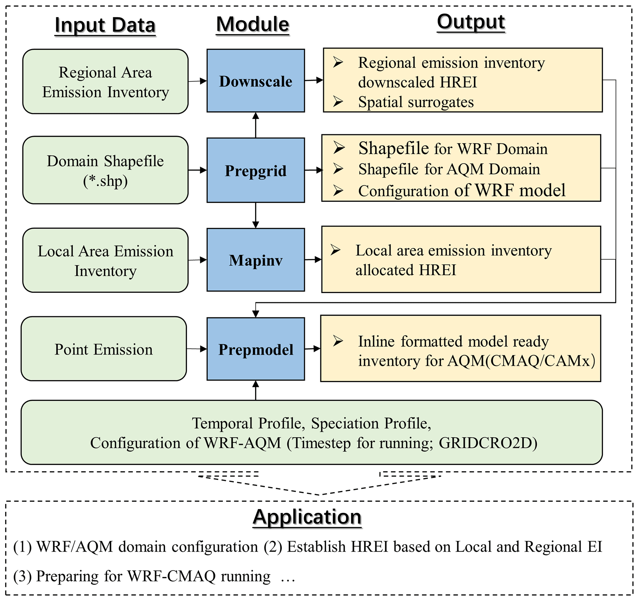
We developed an integrated tool to complete the workflow from a nested-domain configuration to a model-ready HREI for WRF-AQM, as depicted in Fig. 1. The shapefiles provide location and extent in each domain used to configure nested domains in WRF-AQM by the Prepgrid module. For domains without a local emission inventory, REIs such as the MEIC can be downscaled into domains by the Downscale module. Local emission inventories can be allocated into domains by the Mapinv module. Both the CMAQ and CAMx models support inline plume rise calculations and inline-format HREI (Guevara et al., 2014). Based on gridded emissions from Downscale and Mapinv, the inline-format HREI for WRF-AQM can be created in Prepmodel. Users can adopt each module individually or in combination according to their needs. The methodological innovations in this study included a nested-domain configuration algorithm, a sub-grid nearest method, a user-friendly emission source ID, and speciation profiles, as detailed in the following sections.

Figure 1 ISAT framework.

2.1 Nested-domain configuration in Prepgrid

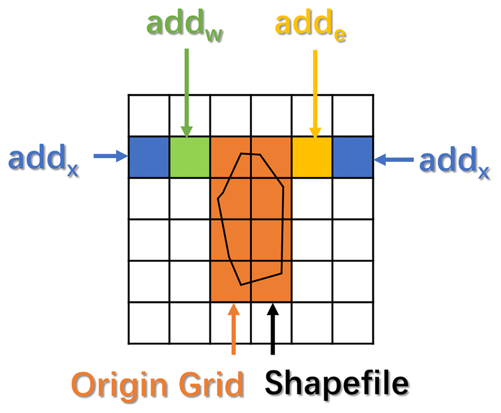
Using Arakawa C-grid staggering in the WRF model, a 3:1 grid-distance nesting ratio between domains is required for a nested-domain configuration (Skamarock et al., 2019). Nested domains can be classified into parent and child domains and initially configured based on the extent of shapefiles (Daniels et al., 2016). The outermost domain determines the projection in WRF-AQM. The child domains need to be extended based on user needs and the 3:1 grid-distance nesting ratio between domains. Users can set the number of extended grids in the east, west, south, and north directions as needed: (add_e, add_w, add_s, and add_n). The number of grids that must be expanded under grid-distance nesting rules were also considered: (add_x and add_y). Taking the x direction as an example, add_e, add_w, and add_x were used to extend the domain in the WRF model, as shown in Fig. 2. Moreover, due to the outermost cells in WRF being inappropriate for use in an AQM (US EPA, 2019), model_clip was conducted to define a lateral boundary for the AQM, as shown in Appendix A. In practice, we usually obtain the extent of the study area based on its shapefile. Compared with manual configuration, using a shapefile can provide a consistent and accurate nested domain between WRF, AQM, and an emission inventory. The major steps and key parameters are described below.

Figure 2 Parameters for modifying the domain in the x direction.

2.1.1 Projection configuration based on the outermost domain

Standard parallels, the central meridian, and the latitude of the Lambert conformal conic (LCC) projection can be obtained from the shapefile in the outermost domain. Due to defined grid spacing, the WRF-AQM domain may exceed the study area's shapefile; thus, the shapefile center does not represent the center of the LCC projection. We designed four main steps to accomplish projection configuration. (i) The first is setting standard parallels. Standard parallels were defined by users according to the location of the outermost domain (for example, Shanxi province configured with 33 and 42^∘). (ii) The second is setting the extent and number of grids in domain. Under the LCC projection in the previous step and the shapefile, we obtained the number of grids (num_x and num_y) and origin (X_min and Y_min) as shown in Eqs. (1)–(4). (iii) The third is updating LCC projection. The center of the domain was transferred into WGS 84 projection and used to update the center in LCC projection. (iv) The fourth is getting final LCC projection parameters, looped through steps (iii)–(ii)–(iii) until the difference in the center of the domain and shapefile in the loops could be ignored.

$$\begin{array}{}\text{(1)}& {\displaystyle }{\mathrm{num}}_x=\mathrm{Roundup}\left({\displaystyle \frac{\mathrm{disx}}{\mathrm{d}x}}\right)+{\mathrm{add}}_{\mathrm{e}}+{\mathrm{add}}_{\mathrm{w}},\text{(2)}& {\displaystyle }{\mathrm{num}}_y=\mathrm{Roundup}\left({\displaystyle \frac{\mathrm{disy}}{\mathrm{d}y}}\right)+{\mathrm{add}}_{\mathrm{s}}+{\mathrm{add}}_{\mathrm{n}},\text{(3)}& {\displaystyle }{X}_{\min }={\displaystyle \frac{-({\mathrm{num}}_x\times \mathrm{d}x)}{\mathrm{2}}},\text{(4)}& {\displaystyle }{Y}_{\min }={\displaystyle \frac{-({\mathrm{num}}_y\times \mathrm{d}y)}{\mathrm{2}}},\end{array}$$

where disx and disy represent the length of the shapefile in the x and y directions.

2.1.2 Determination of child domain parameters

Constrained by grid-distance nesting rules and lateral boundaries for the AQM, the child domain configuration step is different from the parent domain step. Spatial resolution and origin in the parent and child domains (dx_par, dx_child, xstart_child, and xstart_parent) were adopted for the child domain configuration. Taking the x direction as an example, the number of grids was calculated based on the spatial coverage of the shapefile, user-defined parameters, and the number of grids constrained by the nesting rules in the WRF model, as shown in Eq. (5). The term add_x is the must-add number of grids according to the nesting rules and the shapefile in the parent and child domain, as shown in Eq. (6), and num_x was further corrected by Eqs. (7)–(8). X_min is the present start position of the child domain with a projection configuration based on the nesting rules and the user-defined add_w as shown in Eq. (9). Moreover, start_x denotes the starting position for the child domain in the parent domain, which can be used to configure a nested domain in the WRF model in Eq. (10).

$$\begin{array}{}\text{(5)}& {\displaystyle }{\mathrm{num}}_{x,\mathrm{tmp}}=\mathrm{Roundup}\left({\displaystyle \frac{{\mathrm{disx}}_{\mathrm{child}}}{\mathrm{d}{x}_{\mathrm{child}}}}\right)+{\mathrm{add}}_{\mathrm{e}}+{\mathrm{add}}_{\mathrm{w}}+{\mathrm{add}}_x\text{(6)}& {\displaystyle }\begin{array}{rl}& {\mathrm{add}}_x=\\ & \mathrm{Roundup}\left({\displaystyle \frac{{\mathrm{xstart}}_{\mathrm{child}}-\mathrm{int}\left(\frac{{\mathrm{xstart}}_{\mathrm{child}}-{\mathrm{xstart}}_{\mathrm{parent}}}{\mathrm{d}{x}_{\mathrm{par}}}\right)\times \mathrm{d}{x}_{\mathrm{par}}-{\mathrm{xstart}}_{\mathrm{parent}}}{\mathrm{d}{x}_{\mathrm{child}}}}\right)\end{array}\text{(7)}& {\displaystyle }{\mathrm{tmpgrid}}_x=\mathrm{mod}\left({\mathrm{num}}_{x,\mathrm{tmp}},{\displaystyle \frac{\mathrm{d}{x}_{\mathrm{par}}}{\mathrm{d}{x}_{\mathrm{child}}}}\right)\text{(8)}& {\displaystyle }{\mathrm{num}}_x=\left\{\begin{array}{l}{\mathrm{num}}_{x,\mathrm{tmp}}({\mathrm{tmpgrid}}_x=\mathrm{0})\\ {\mathrm{num}}_{x,\mathrm{tmp}}+\frac{\mathrm{d}{x}_{\mathrm{par}}}{\mathrm{d}{x}_{\mathrm{child}}}-{\mathrm{tmpgrid}}_x({\mathrm{tmpgrid}}_x\ne \mathrm{0})\end{array}\right.\text{(9)}& {\displaystyle }\begin{array}{rl}{X}_{\min }& =\mathrm{integer}\left({\displaystyle \frac{{\mathrm{xstart}}_{\mathrm{child}}-{\mathrm{xstart}}_{\mathrm{parent}}}{\mathrm{d}{x}_{\mathrm{par}}}}\right)\times \mathrm{d}{x}_{\mathrm{par}}\\ & +{\mathrm{xstart}}_{\mathrm{parent}}-\mathrm{d}{x}_{\mathrm{child}}\times {\mathrm{add}}_{\mathrm{w}}\end{array}\text{(10)}& {\displaystyle }{\mathrm{start}}_x={\displaystyle \frac{X_{\min }-{\mathrm{xstart}}_{\mathrm{parent}}}{\mathrm{d}{x}_{\mathrm{par}}}}\end{array}$$

2.2 Sub-grid nearest method in Downscale

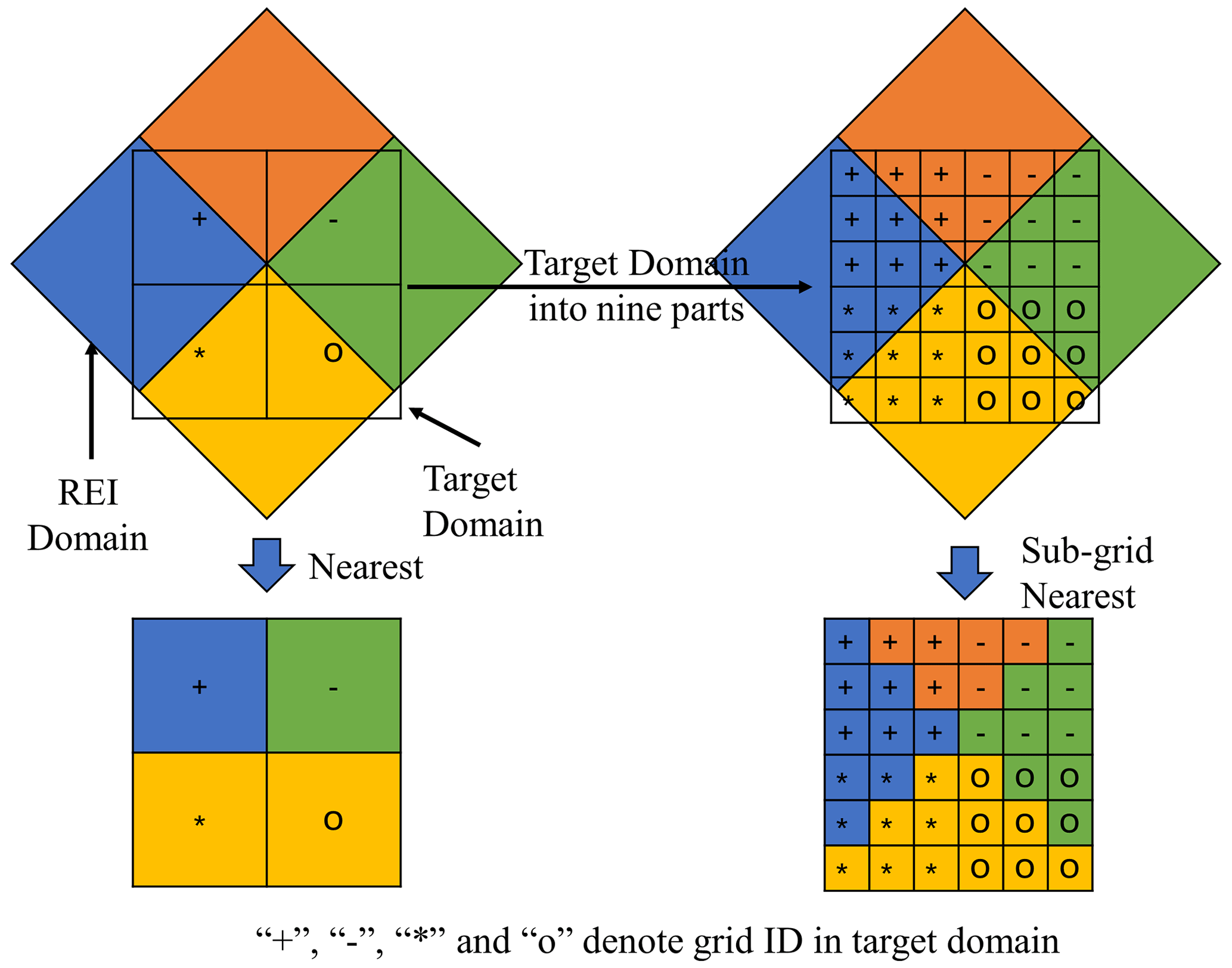
Intersect and nearest methods are commonly used to downscale REI into user-defined domains. The intersect method obtains overlapping areas between the REI and the target domain, while the nearest method assigns emissions based on the nearest REI value. The intersect method accurately reflects the spatial relationship between the target domain and the REI. However, if there are evident projection and spatial resolution differences between REI and the target domain, a large number of small intersections are created, which significantly decreases calculation efficiency. The nearest method addresses this limitation but may lead to emission mismatches due to spatial differences. For example, the nearest method ignored the orange grid emissions but exaggerated the contribution of the yellow grids in the research domain, as shown in Fig. 3. To fully consider the advantages and disadvantages of these two algorithms, we used the sub-grid nearest method to allocate the emission inventory, as shown in Eqs. (11)–(13). Figure 3 depicts the process we used to obtain the REI values using the nearest and sub-grid nearest methods. The colors in the figure represent the REI values, and the symbols (such as ^*) represent the grid ID. First, we introduced a “sub-grid ratio” to divide each grid into p sub-grids, such as nine sub-grids in each grid. Second, we adopted the conventional nearest method to locate the nearest REI values for each sub-grid. Third, we calculated the emissions for each sub-grid based on the nearest REI value and spatial surrogates. Finally, we obtained the emissions for each grid based on a summary of the sub-grid emissions in each grid. It should be ensured that ${\mathrm{SA}}_{\mathrm{region},I_{i,j,p}}$ is larger or equal to the sum of ${\mathrm{SA}}_{\mathrm{target},i,j,p}$ in the same region grid $I_{i,j,p}$ based on the principle of mass conservation. This module can downscale regional emission inventories in a user-friendly and easy-to-use way based on a default or user-defined proxy without external tools such as ArcGIS.

$$\begin{array}{}\text{(11)}& {\displaystyle }{E}_{\mathrm{target},i,j}={\sum }_p{E}_{\mathrm{target},i,j,p},\text{(12)}& {\displaystyle }\begin{array}{rl}{E}_{\mathrm{target},i,j,p}& =E_{\mathrm{region},I_{i,j,p}}\times R_{\mathrm{region},I_{i,j,p}}\\ & \times {\displaystyle \frac{{\mathrm{SA}}_{\mathrm{target},i,j,p}}{{\mathrm{SA}}_{\mathrm{region},I_{i,j,p}}}},\end{array}\text{(13)}& {\displaystyle }{I}_{i,j,p}=\mathrm{Nearest}({\mathrm{Grid}}_{\mathrm{target},i,j,p},{\mathrm{Grid}}_{\mathrm{region}}),\end{array}$$

where i and j are the column and row number of the target grid, p is the sub-grid ID in grid (i,j), $E_{\mathrm{target},i,j}$ is the emissions in grid (i,j), $E_{\mathrm{target},i,j,p}$ is the emissions in sub-grid p in grid (i,j), $I_{i,j,p}$ is the location of sub-grid p for the target grid (i,j) in the region domain, $E_{\mathrm{region},I_{i,j,p}}$ represents the regional emissions in $I_{i,j,p}$, ${\mathrm{SA}}_{\mathrm{region},I_{i,j,p}}$ is the spatial allocator for region grid $I_{i,j,p}$, ${\mathrm{SA}}_{\mathrm{target},i,j,p}$ is the spatial allocator for sub-grid p of target grid (i,j), Grid_region is the domain of the REI, and ${\mathrm{Grid}}_{\mathrm{target},i,j,p}$ is the sub-grid p of target grid (i,j); ${\mathrm{R}}_{\mathrm{region},I_{i,j,p}}$ is an adjustment factor to ensure mass conservation.

Figure 3 Concept of the sub-grid nearest method.

2.3 User-friendly emission source sector ID in Prepmodel

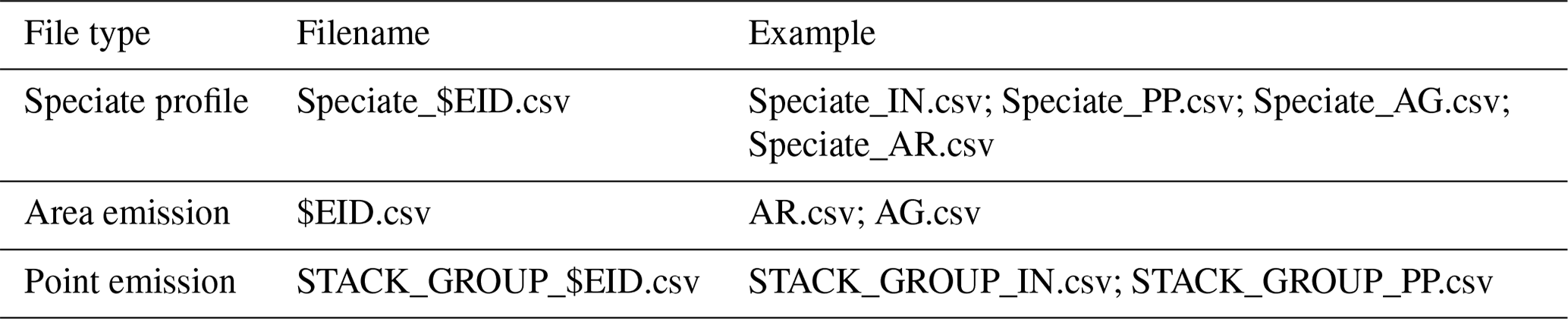
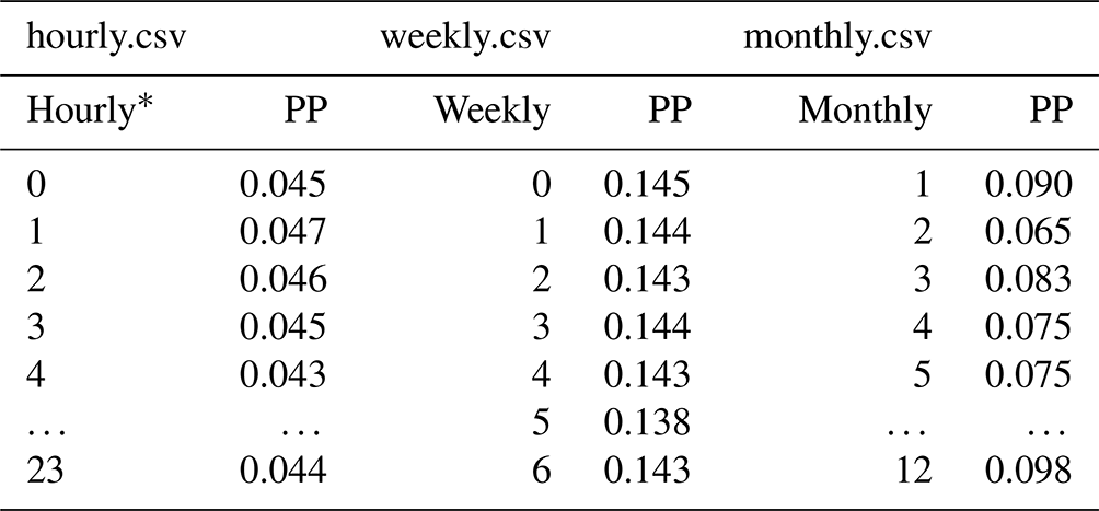
User-friendly emission source sector IDs (EIDs) are source abbreviations: for example, AG for agriculture. The EID is a unique ID for the emission source sector in ISAT. Speciate and temporal profiles for sectors can be easily defined with an EID, as shown in Table 1, where the speciate profile and point emission inventory are prefixed by Speciate_ and STACK_GROUP_ and suffixed by an EID. The area emission inventory was called EID. To define a temporal profile for each sector, users can add columns labeled by EID in hourly.csv, weekly.csv, and monthly.csv, as shown in Table 2. Users can easily add or delete sources in a model-ready emission inventory according to their needs in Prepmodel.

Table 1 File structure defined by emission source sector ID (EID).

Table 2 Case of temporal profiles (for PP source).

^* UTC.

2.4 User-friendly speciation profile structure in Prepmodel

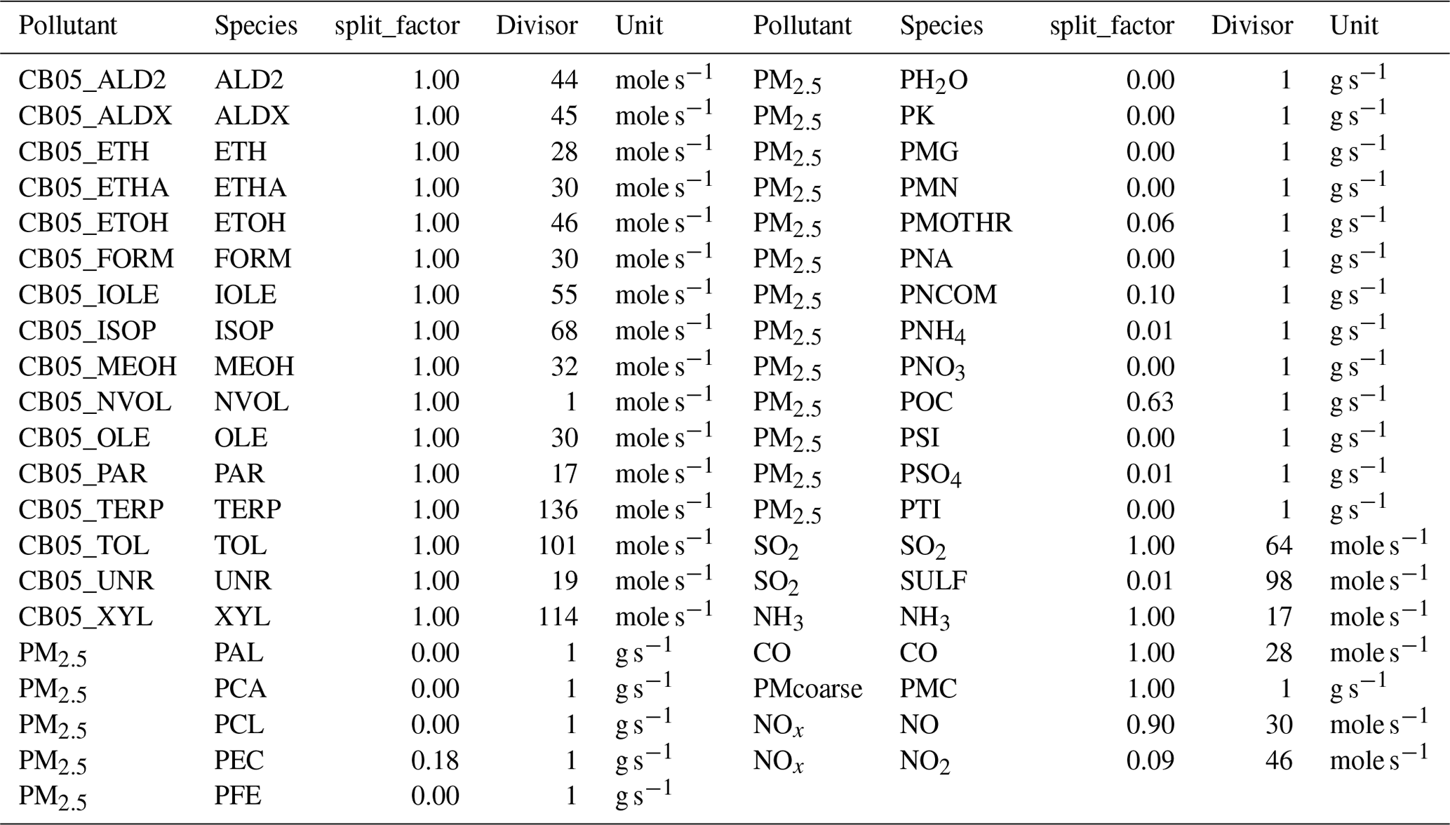
Compared with multiple input file types for chemical speciation in the SMOKE model, including GSCNV, GSPRO, GSPRODESC, GSPRO_COMBO, GSREF, and GSTAG files, this tool simplifies the process with individual speciate profiles for each sector. An example of a speciate profile is shown in Table 3. Here, “pollutant” denotes the pollutants in the emission inventory, “species” denotes the pollutants in the chemical mechanism adopted in the AQM, “split_factor” represents the fraction of the pollutant emission to species in the AQM between zero and 1 (and it must be mass-conservative), “unit” is the unit of species adopted in the AQM (such as “moles/s” for gaseous pollutants and “g/s” for particulate pollutants), and “divisor” converts mass-based speciation into mole-based speciation, with molar mass for gaseous pollutants and a default value (set to 1) for particulate pollutants. Therefore, the user can easily modify the speciation profile based on the chemical mechanism in the AQM and the pollutants in the emission inventory.

Table 3 Case of speciate profile in ISAT.

In addition, we embedded a gridded spatial surrogate for roads and populations in the ISAT. The road database was obtained from OpenStreetMap, with four levels, including motorway, secondary road, primary road, and residential road. The standard road length (Zheng et al., 2009), based on vehicle speed, number of lanes, and road width from the Code for Transport Planning on Urban Roads (GB 50220-95) in China, was used to calculate the gridded road map data. Population density data based on the 2020 LandScan Global Population Database (Rose et al., 2021) can be used in ISAT with NetCDF. Users can also prepare any proxy for their needs. For example, land use and point of interest (POI) data are recommended for agriculture and residential sectors (Wang et al., 2017; Huang et al., 2022). Due to the nearly 1 km resolution of the ISAT-embedded gridded population and road maps, users can generate HREIs with finer spatial resolution ≥1 km.

3 Case studies

As the capital of China, Beijing has a large population and number of vehicles, making it a hotspot for air pollution research in China (Gao et al., 2018; X. Huang et al., 2021). This study presents three nested-domain cases: mainland China, Beijing–Tianjin–Hebei (BTH), and Beijing (BJ), with spatial resolutions of 27, 9, and 3 km, respectively, as shown in Fig. 4. The ISAT was used for the workflow from the nested-domain configuration to the model-ready inventory for the WRF-AQM. The shapefile for these domains was used to configure nested domains in the WRF-AQM and to create the ready emission inventory in the Prepgrid module. Provincial pollutant sources in transportation and residential sectors in Beijing (BMEE, 2021) were allocated into 3 km × 3 km grids by the Mapinv module. The MEIC regional emission inventory with a spatial resolution of 0.25^∘ × 0.25^∘ in 2020 was downscaled to grid level in the Downscale module.

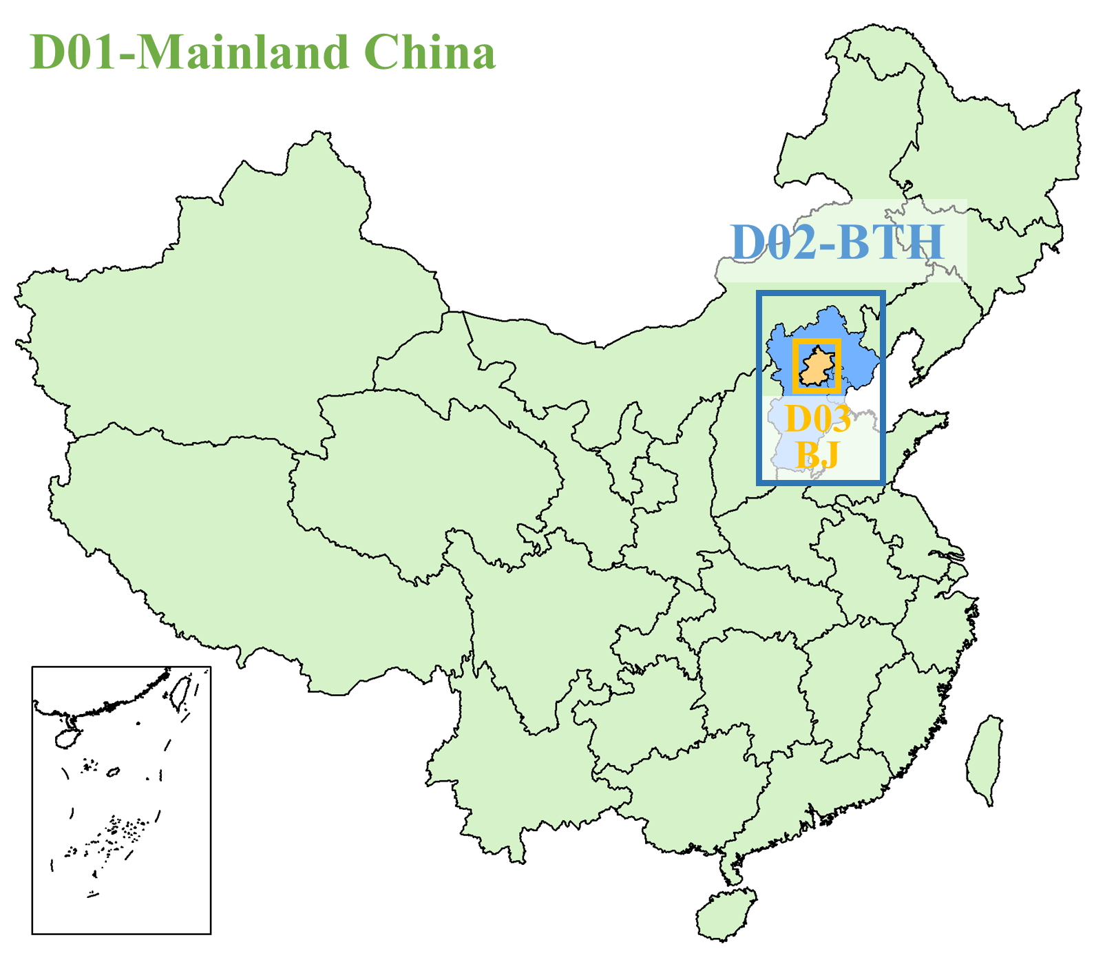
Figure 4 The three nested domains and their shapefiles.

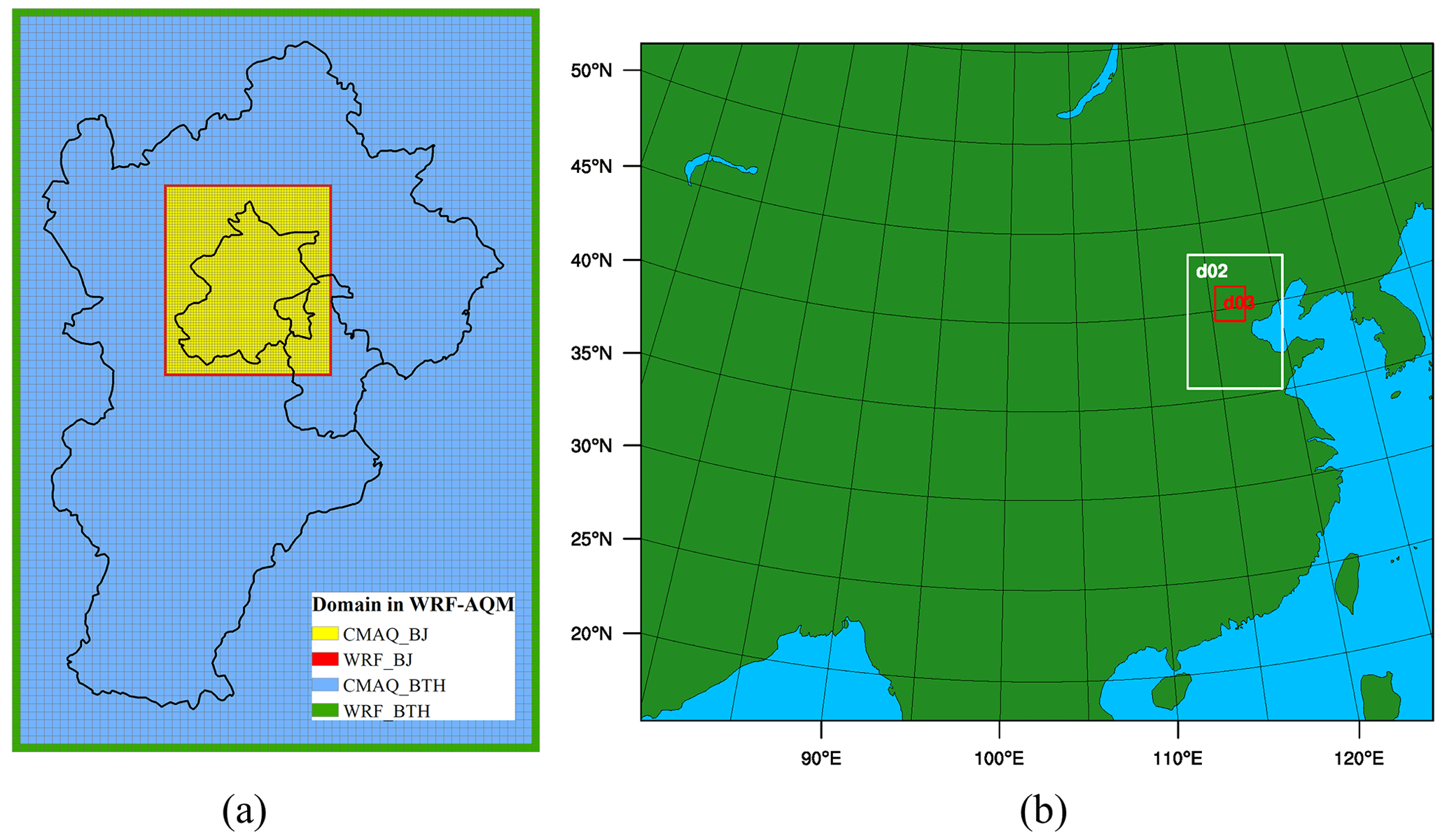
Figure 5 ISAT-configured WRF-AQM nested domains.

3.1 Nested-domain configuration by Prepgrid

ISAT provides comprehensive grid information for the WRF-AQM in comma-separated value (.csv) files and shapefile formats. Data formatted in .csv contain grid information for each domain and can be further used as the input for other ISAT modules. Shapefile-formatted data can be displayed directly in ArcGIS or other geographic information system to display and check the configuration for nested domains. “Domainname” and “Casename” were used to mark the output in the Prepgrid module. “${Casename}_gridinfo.csv” summarizes grid information in nested domains and can be used to configure domain parameters in the WRF model, as shown in Fig. 5b. “wrf_${Domainname}.shp” and “wrf_${Domainname}.csv” provided shapefile and grid information for the ISAT-configured WRF model. “aqm_${Domainname}.shp” and “aqm_${Domainname}.csv” were the shapefile and grid information for the ISAT-configured AQM. Due to the blend of larger-scale driving data and scale-specific physics, the outermost cells in the WRF domain are inappropriate to use and usually removed in AQM (US EPA, 2019). The ISAT-configured domains reflect this requirement of a lateral boundary in AQM and accurately obtain the WRF-AQM domain.

3.2 Downscaled regional emissions inventory by Downscale

The MEIC inventory is widely used in China. In this study, the 2020 annual MEIC emissions were preprocessed into .csv format and downscaled into the AQM domain by the Downscale module. Compared with ArcGIS, SMOKE, and other tools, using the Downscale module reduces the timeliness from hours to minutes. We compared gridded residential emissions in BTH under different downscaled method, including the intersect method, nearest method, and sub-grid nearest method. The sub-grid ratio, the key parameter in the sub-grid nearest method, must either be 1 or a multiple of 3 and applied to test the allocation result. Therein, the nearest method can be configured with a sub-grid ratio equal to 1. With the sub-grid ratio increased from 1 to 9, the spatial allocation was close to the result of the intersect method for the urban area, as shown in Fig. 6. The sub-grid method with a sub-grid ratio equal to 3 significantly improved the allocation compared to the nearest method, and the R-squared increased from 0.91 to 0.98. The increase in the sub-grid ratio from 3 to 9 slightly improved the distribution results, with R-squared increasing from 0.979 to 0.984, as shown in Fig. 7. Although a higher sub-grid ratio may lead to a more accurate allocation, one needs to consider the computational efficiency and resolution of the spatial surrogate. For example, the running time of the “downscaled” module increased from 2 to 10 min, and the sub-grid ratio increased from 3 to 9 in this case. In addition, for REI grids with empty spatial surrogates, ISAT applies the grid area as a weight when allocating emissions. Constrained by the spatial surrogate (≤1) for each REI grid based on the principle of mass conservation, the downscaled emission inventory exhibited good agreement with the REI. Regarding the result of the intersect method as the true value, the relative error of total PM_2.5 emissions under each sub-grid ratio is less than 0.2 %, which reflects the good quality of the downscaling in terms of mass flux conservation.

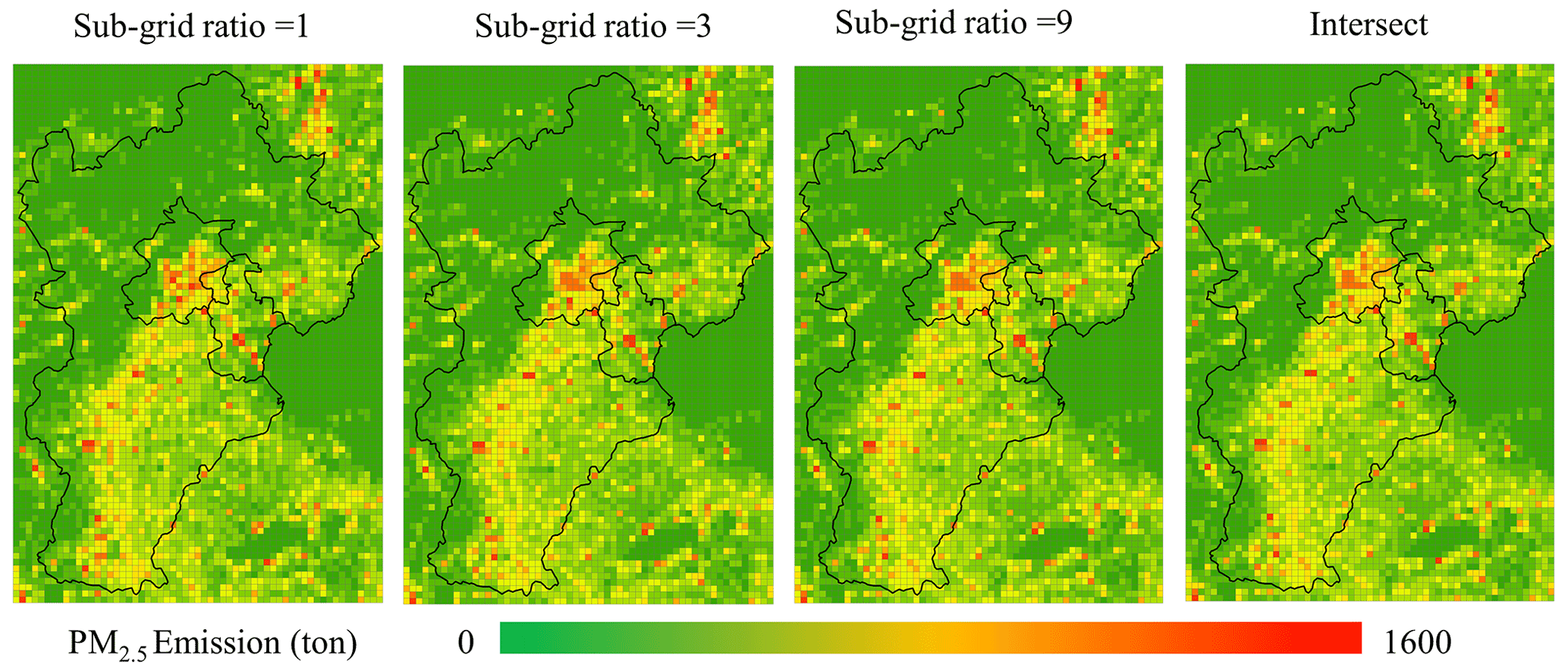
Figure 6 Comparison of the intersect and the sub-grid nearest method allocations with different sub-grid ratios.

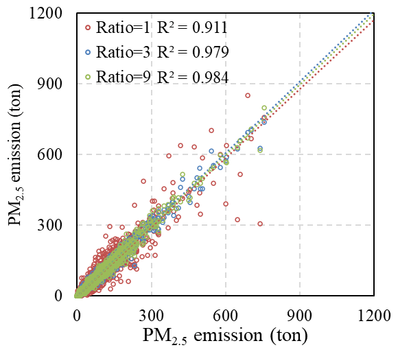
Figure 7 Pairwise relationship between the intersect and sub-grid nearest methods with different sub-grid ratios for particulate matter (PM).

These downscaled REIs can be used to produce model-ready emissions for domains without a local emission inventory. Due to more detailed and realistic emission characteristics, a local emission inventory is highly recommended based on spatial–temporal emission characteristic research and simulation in WRF-AQM in the innermost domain.

3.3 Gridded local emission inventory by Mapinv

Differing from the downscale process used for the gridded REI described in Sect. 3.2, mapping the provincial- and/or city-level local emission inventory onto the grid level required the identification of region attributes for each AQM domain and the allocation of emissions based on spatial surrogates. In ISAT v2.0, users can add a column to define the region in the shapefile and input the local emission inventory in the “localinv” file. ISAT will allocate the local emission inventory for each species to grid level. Taking Beijing as an example, emissions for the occupied residential (RE) and transportation sectors were 7763 t NO_x with 25 900 t VOCs and 22 700 t NO_x with 2654 t VOCs, respectively. The gridded emission inventory for the occupied residential (RE) and transportation (TR) sectors created by the ISAT reflected the spatial variations in population density and the road map in Beijing, as shown in Fig. 8. Based on the embedded population density and road map, ISAT could flexibly allocate the local emission inventory to grid level.

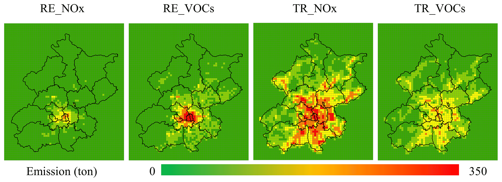
Figure 8 Spatial allocation for Beijing.

3.4 Model-ready emission inventory by Prepmodel

Users can generate inline-format model-ready emission inventories for AQM using the Prepmodel module. The gridded emission inventory generated by Mapinv and Downscale can be used as area emission input files. The point emission file was organized into .csv format, which contained emissions, locations, and stack parameters with reference to the SMOKE model. Temporal profile files were defined based on statistical data and previous studies. The speciation profiles for sectors were obtained from the SPECIATE database or field measurements. Moreover, GRIDCRO2D files generated by the Meteorology–Chemistry Interface Processor in the CMAQ model were applied to provide global attributes and configurations consistent with the AQM. “Runtime” was used to define the model-ready emission time steps for the AQM. The ISAT inline-format emission inventory was named EID. For example, “TR.nc” denoted the area emission source for the TR sector. “PPpoint.nc” and “STACK_GROUP_PP.nc” represented hourly emissions and the source information for the power plants, respectively. The model-ready emission inventory can be directly used in AQMs, such as CMAQ and CAMx, as well as instrumental modules, such as the decoupled direct method (DDM) and integrated source apportionment method (ISAM). Previous studies achieved reliable simulation results using this approach (H. Wang et al., 2021; K. Wang et al., 2022a, 2021a, b; Liu et al., 2023; Li, 2021; Tan, 2022).

The configurations and steps used in these cases are detailed in Appendix A.

4 Conclusion

We have developed an integrated tool, ISAT v2.0, that streamlines the workflow from a nested-domain configuration to a model-ready emission inventory for WRF-AQM. ISAT v2.0 consists of four main modules: Prepgrid, Downscale, Mapinv, and Prepmodel. The Prepgrid module can accurately provide user-defined domain configuration under nesting rules in WRF-AQM and the shapefile of the study area. It can also configure the namelist.wps file in WPS using domain parameters defined in this module. The Downscale module conducted with the “sub-grid nearest” method significantly improved the allocation result in comparison to the Downscale module with the nearest method. Moreover, users can flexibly set the “sub-grid ratio” according to their specific needs. The Mapinv module provides a user-friendly tool to allocate a provincial- and/or city-level local emission inventory to grid level using user-defined shapefiles and local emission inventories. Finally, the Prepmodel module can generate an inline-format model-ready file emission inventory for WRF-AQM and provides users with the numerical simulations. ISAT is free, expansible, and supported by both Linux and Windows, and it can be applied to process other regional emission inventories, such as REAS, by providing grid templates and updating user-defined spatial surrogates. Relying on the established relationship between the shapefile and the WRF-AQM domain, ISAT is highly extendable, including the creation of ocean files in CMAQ models (US EPA, 2019), the labeling of source regions in CAMX-PSAT, and other potential uses.

Appendix A: ISAT step-by-step guide

Taking the nested domains in Fig. 4 with a spatial resolution of “27km-9km-3km” as an example.

Step 1: obtain nested-domain parameters for WRF-AQM based on the domain shapefile

(a) Give the information of “par.ini” in the Prepgrid module

lat1:33.0	# First standard latitude for LCC
lat2:42.0	# Second standard latitude for LCC
casename:3nestdomain	# Case name
numdom:3	# Number of nested domains
shpath: ./shp/mainlandchina.shp, ./shp/JJJ.shp,./shp/beijing.shp	# Shpfile path for domains
dx:27000,9000,3000	# Resolution in meters for domains
xladd:2,3,3	# Added grid in left in x direction
xradd:2,3,3	# Added grid in right in x direction
ytadd:2,3,3	# Added grid in top in y direction
ydadd:2,3,3	# Added grid in down in y direction
domainname:MainlandChina,JJJ,Beijing	# Name for domains
model_clip:1,1,1	# Clip number of grids for AQM

(b) Running the Prepgrid module by “python prepgrid.py” – domain information summarized in “3nestdomain_gridinfo.csv”, detailed below

domid	centlon	centlat	xmin	ymin	numx	numy	xstart	ystart
0	102.0737	36.68731	−2 484 000	−2 119 500	184	157	0	0
1	102.0737	36.68731	945 000	−40 500	66	93	127	77
2	102.0737	36.68731	1 116 000	382 500	63	72	19	47

Therein, you can define the WPS domain the using variables above
parent_id	1	1	2
parent_grid_ratio	1	3	3
i_parent_start	1	$xstart(1) + 1	$xstart(2) + 1
j_parent_start	1	$ystart(1) + 1	$ystart(2) + 1
e_we	$numx(0) + 1	$numx(1) + 1	$numx(2) + 1
e_sn	$numy(0) + 1	$numy(1) + 1	$numy(2) + 1
ref_lat	$centlat
ref_lon	$centlon
truelat1	$lat1
stand_lon	$centlon
truelat2	$lat2

(c) You can get a fishnet shapefile for the WRF model called “wrf_” + ${domainname} + “.shp” and AQM called “aqm_” + $domainname + “.shp”

(d) You can also get gridded information for domains in “wrf_” + ${domainname} + “.csv” for the WRF model and “aqm_” + $domainname+ “.shp” for AQM, respectively

Step 2: downscaling regional emission inventory into target domains

(a) Give the information of “par.ini” in the Downscale module

invf:./input/domain/aqmJJJ.csv	# Path of target domain information
dx:9000	# Resolution in meters for target domain
ratio:3	# Sub-grid ratio
emissions: ./regioninv/agricultureannual.csv,./regioninv/transportationannual.csv,./regioninv/residentialannual.csv	# Path for regional emission inventory
casename:JJJ	# Case name
method:area,road,pop	# Allocation method for specific emission inventory area: based on grid area road: based on roads map pop: based on population map

(b) Running the Downscale module by “python downscale.py” and getting gridded emissions for specific area sources

Step 3: preparation of model-ready emission inventories for AQM

(a) Give the information of “par.ini” in the Prepmodel module

runtime:193	# Time steps for AQM run
gridcro2d: ./src/met/GRIDCRO2D_9km	# MCIP generated GRIDCRO2D file
speciate: ./src/speciate/speciate_AR.csv, ./src/speciate/speciate_AG.csv	# Speciation profile for area emission sources.
speciate_groups: ./src/speciate/speciate_IN.csv	# Speciation profile for point emission sources.
temporary_hour : ./src/temporary/hourly.csv	# Hourly temporal profile for emission sources.
temporary_week : ./src/temporary/weekly.csv	# Weekly temporal profile for emission sources.
temporary_month: ./src/temporary/monthly.csv	# Monthly temporal profile for emission sources.
emissions: ./src/emissions/MEIC/AR.csv, ./src/emissions/MEIC/AG.csv	# Path of area emission files
stack_groups: ./src/emissions/MEIC/STACK_GROUP_IN.csv	# Path of point emission files

(b) Run the Prepmodel module by “python area_emis.py; python point_emis.py; python point_info.py” – for the CAMx model, CMAQ2CAMx can be used transfer this output into CAMx

Other step: mapping a local emission inventory to the grid level

(a) Give the information of “par.ini” in the Mapinv module

regionshp:./input/Region/BJ.shp	# Shapefile for region
Key:NAME	# Region column in shapefile
grid:./input/Grid/3km.csv	# Grid information by “pregrid”
sapath:./input/SA/inv_sa_tmp_ road.csv,./input/SA/inv_ sa_ tmp_pop.csv	# Spatil surrogated by “downscale” module
localinv:./input/localinv/TR.csv,./input/localinv/RE.csv	# Path way for local emission inventory
localname:TR3KM,AR3KM	# Name of gridded emission inventory output

(b) Run the Mapinv module by “python mapinv.py”