the Creative Commons Attribution 4.0 License.
the Creative Commons Attribution 4.0 License.
 | 27 Mar 2023
Fast approximate Barnes interpolation: illustrated by Python-Numba implementation fast-barnes-py v1.0
Bruno K. Zürcher
Barnes interpolation is a method that is widely used in geospatial sciences like meteorology to remodel data values recorded at irregularly distributed points into a representative analytical field. When implemented naively, the effort to calculate Barnes interpolation depends on the product of the number of sample points N and the number of grid points W×H, resulting in a computational complexity of . In the era of highly resolved grids and overwhelming numbers of sample points, which originate, e.g., from the Internet of Things or crowd-sourced data, this computation can be quite demanding, even on high-performance machines.
This paper presents new approaches of how very good approximations of Barnes interpolation can be implemented using fast algorithms that have a computational complexity of . Two use cases in particular are considered, namely (1) where the used grid is embedded in the Euclidean plane and (2) where the grid is located on the unit sphere.
- Article
(6360 KB) - Full-text XML
- BibTeX
- EndNote


In the early days of numerical weather prediction, various methods of objective analysis were developed to automatically produce the initial conditions from the irregularly spaced observational data (Daley, 1991), one of which was Barnes interpolation (Barnes, 1964). However, objective analysis soon lost its significance in this field against statistical approaches. Today, the Barnes method is still used to create grid-based isoline visualizations of geospatial data, like in the meteorological workstation project NinJo (Koppert et al., 2004) for instance, which is jointly developed by the Deutscher Wetterdienst, the Bundeswehr Geophysical Service, MeteoSwiss, the Danish Meteorological Institute and the Meteorological Service of Canada.
Barnes interpolation for an arbitrary point x∈D and a given set of sample points xk∈D with observation values fk∈ℝ for is defined as
with Gaussian weights
a distance function and a Gaussian width parameter σ.
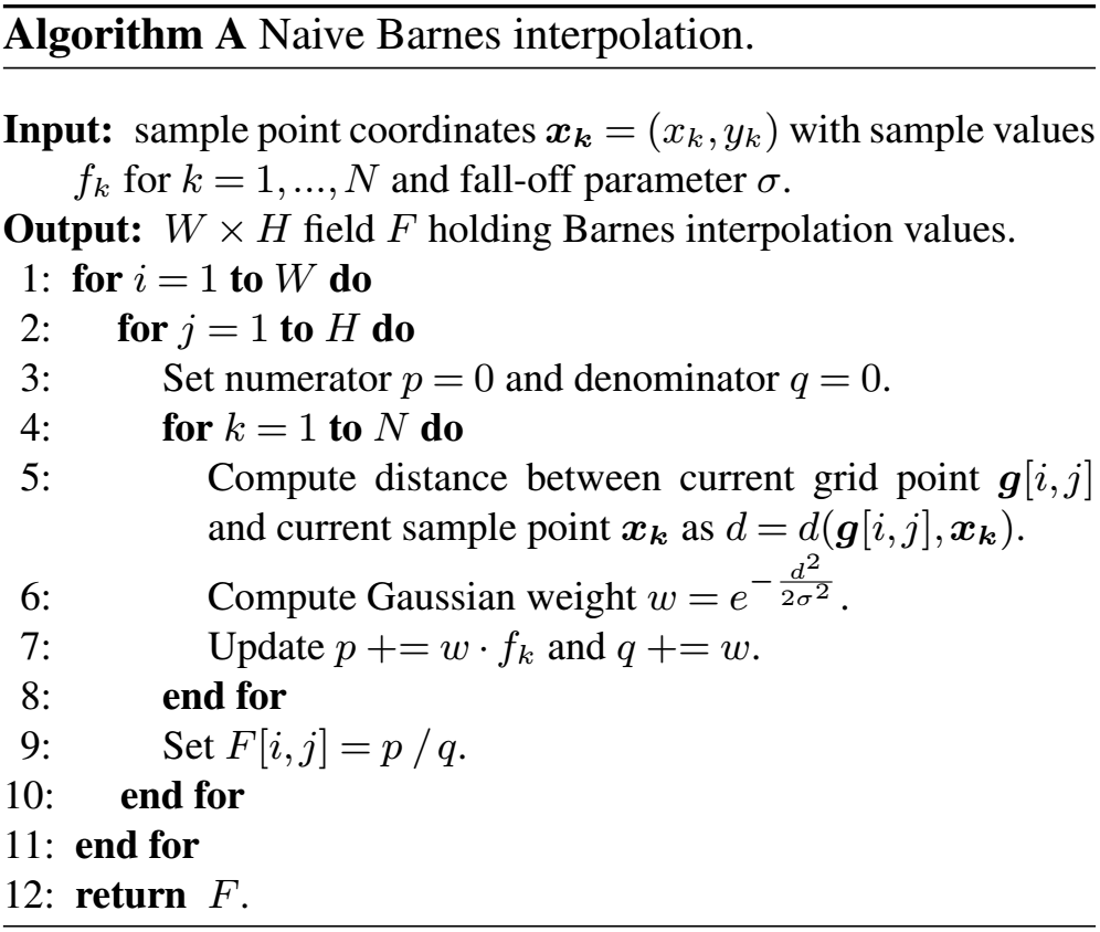
If Barnes interpolation is computed in a straightforward way for a regularly spaced W×H grid, the computational complexity is given by as easily can be seen from the 3-fold nested loops of Algorithm A given below. Consequently, for big values of N or dense grids, a naive implementation of Barnes interpolation turns out to be unreasonably slow.
The fact that the Gaussian weight function quickly approaches 0 for increasing distances leads to a first improvement attempt, which consists of neglecting all terms in the sums of Eq. (1), for which the weights wk drop below a certain limit w0, e.g., w0=0.001. This is equivalent to only taking into account observation points xk that lie within the distance from the interpolation point x. Thus, the described procedure requires the ability to quickly extract all observation points xk that lie within a distance r0 from point x. Data structures that support such searches, e.g., are so-called k–d trees (Bentley, 1975) or quadtrees (Finkel and Bentley, 1974).
This improved approach actually reduces the required computational time by a constant factor, but the computational complexity remains in the same order. To see this, note that a specific sample point xk contributes to the interpolation value of exactly those grid points that are contained in the circular disk of radius r0 around it. Also note that in a regularly spaced grid, the number of affected grid points is roughly the same for each sample point. If now the number of grid points W and H in each dimension is increased by a factor of κ – i.e., the grid becomes denser – the number of grid points contained in grows accordingly, namely by a factor of κ2, which shows that the algorithmic costs rise in direct dependency to W and H. Since this is obviously true for the number of sample points N as well, the improved algorithm also has complexity .
In this paper, we discuss a new and fast technique to compute very good approximations of Barnes interpolation. The utilized underlying principle of applying multiple convolution passes with a simple rectangular filter in order to approximate a Gaussian convolution is well known in computational engineering. In image processing and computer vision, for instance, Gaussian filtering of images is often efficiently calculated by repeated application of an averaging filter (Wells, 1986).
The theoretical background of the new approach is presented in Sects. 2 and 3. Thereafter, we investigate two use cases for the domain D:
For a set of independent and identically distributed (i.i.d.) random variables with mean μ and variance σ2, the central limit theorem (Klenke, 2020) states that the probability distribution of their sum converges to a normal distribution if n approaches infinity, formally written as
Without loss of generality, we assume in the further discussion that μ=0. Let p(x) denote the probability density function (PDF) of the scaled random variables that consequently have the variance . Since the PDF of a sum of random variables corresponds to the convolution of their individual PDFs, we find that on the other hand
where p∗n(x) denotes the n-fold convolution of p(x) with itself (refer to Appendix A). With that result, we can write the relationship (3) equivalently in an unintegrated form as
which leads directly to
Approximation 1. For sufficiently large n, the n-fold self-convolution of a probability density function p(x) with mean μ=0 and variance approximates a Gaussian with mean 0 and variance σ2, i.e.,
Note that this approximation is valid for arbitrary PDFs p(x) with mean μ=0 and variance .
A particularly simple PDF is given by the uniform distribution. We therefore define a family of uniform PDFs as , of which each member un(x) has mean 0 and variance . These uniform PDFs can be expressed by means of elementary rectangular functions:
such that
where . From this definition, it is clear that un(x) is actually a PDF with mean E[un]=0 and variance
as postulated. According to the convergence relation (4) and Approximation 1, the series of the n-fold self-convolutions converges to a Gaussian with mean 0 and variance σ2. The converging behavior can actually be examined visually in Fig. 1, which plots the n-fold self-convolution of the first few family members.
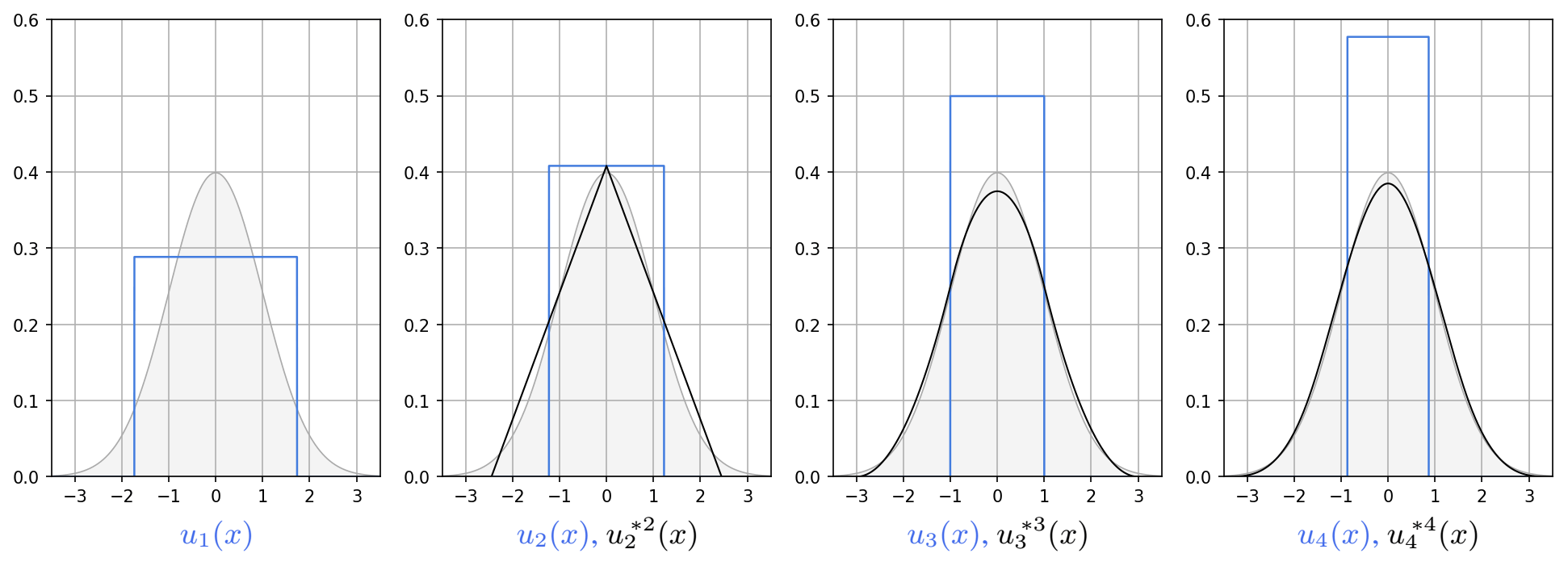
Figure 1From left to right, blue indicates the plot of the PDFs of the uniform distributions u1(x), u2(x), u3(x) and u4(x) for σ=1; black shows their self-convolutions , and . The area covered by the PDF of the normal distribution is indicated in gray.
The central limit theorem can also be stated more generally for i.i.d. m-dimensional random vectors , refer for instance to (Muirhead, 1982; Klenke, 2020). Supposing that the Xk has a mean vector μ=0 and a covariance matrix Σ, we can follow the same line of argument as in the one-dimensional case. Let p(x) be the joint PDF of the scaled random variables , which therefore have a zero mean vector and the covariance matrix . Then the limit law in m dimensions becomes
For the remainder of the discussion, we fix the number of dimensions to m=2 and for the sake of readability, we write the vector argument x in its component form (x,y), if it is appropriate. In case the random vectors Xk are isotropic, i.e., do not have any preference in a specific spatial direction, the covariance matrix is a multiple of the identity matrix Σ=σ2I and, in two dimensions, the limit law simplifies to the following:
In the following step, we are aiming to substitute p(x) with the members of the family of two-dimensional uniform distributions over a square-shaped domain, which are defined as
With this definition, the members have a mean vector 0 and an isotropic covariance matrix , and hence satisfy the prerequisite of the limit law in Eq. (6). Also note that is separable because . As a consequence of the latter, the n-fold self-convolution of is itself separable, i.e.,
where the operators and denote one-dimensional convolution in the x and y direction, respectively (refer to Appendix B). Substituting p(x) in Eq. (6) with the right-hand side (RHS) of Eq. (7), we obtain
or expressed as
Approximation 2. For sufficiently large n, the n-fold self-convolution of the two-dimensional uniform probability density function approximates a bivariate Gaussian with mean vector 0 and covariance matrix σ2I, i.e.,
where rn(x) is an elementary rectangular function defined as
Let φμ,σ(x) denote the PDF of a two-dimensional normal distribution with mean vector μ and isotropic variance σ2, i.e.,
Note that φ0,σ(x) corresponds to the RHS of Approximation 2. Further, let δa(x) denote the Dirac or unit impulse function at location a with the property . Then we can write
Thus, a Gaussian-weighted sum as found in the numerator of Barnes interpolation (1) for the Euclidean plane ℝ2 can be written as convolutional operation
and due to the distributivity and the associativity with scalar multiplication of the convolution operator, Eq. (8) follows:
Substituting φ0,σ(x) with Approximation 2, we obtain the following for sufficiently large n:
For the denominator of Barnes interpolation (1), we can use the same expression but set the coefficients fk to 1.
Since the common factors in the numerator and the denominator cancel each other, we can state
Approximation 3. For sufficiently large n, Barnes interpolation for the Euclidean plane ℝ2 can be approximated by
provided that the quotient is defined.
In other words, Barnes interpolation can very easily be approximated by the quotient of two convolutional expressions, both consisting of an irregularly spaced Dirac comb, followed by a sequence of convolutions with a one-dimensional rectangular function of width , executed n times in the x direction and n times in the y direction. As the convolution operation is commutative, the convolutions can basically be carried out in any order. The sequence shown in Approximation 3, evaluated from left to right, is however especially favorable regarding the computational effort.
Approximation 3 can be stated in a more generalized context as well, i.e., also for non-uniform PDFs. In the special case of using a normal distribution with mean 0 and variance σ2, we can even formulate a convolutional expression that is equal to Barnes interpolation. Refer to Appendix C for more details.
In a straightforward way, Approximation 3 leads to a very efficient algorithm for an approximate computation of Barnes interpolation on a regular grid Γ that is embedded in the Euclidean plane ℝ2. Let
be a grid of dimension W×H with a grid-point spacing Δs. Without loss of generality, we assume that all sample points xk are sufficiently well contained in the interior of Γ. In what follows, we differentiate discrete functions from their continuous function counterparts by enclosing the arguments in brackets instead of parentheses and write, for instance, g[i] for g(x) in the one-dimensional case and g[i,j] for g(x,y) in the two-dimensional case.
In an iterative procedure, we now compute the convolutional expression that corresponds to the numerator (or denominator) of Approximation 3 simultaneously for all points [i,j] of grid Γ. The intermediate fields that result from this iteration are denoted by F(m), where m indicates the iteration stage.
The first step consists of discretizing the expression , i.e., by injecting the values fk at their respective sample points xk into the underlying grid. For this purpose, the field F(0) is initialized with 0. From the definition of Dirac's impulse function in two dimensions,
we deduce for its discrete version that the grid cell containing the considered sample point receives the weight , while all other cells are left unchanged with weight 0.
Since a sample point xk in general does not coincide with a grid point (refer also to Fig. 2) and in order to achieve a good localization, the Dirac impulse is distributed in a bilinear way to its four neighboring grid points according to step 5 of Algorithm B.1.
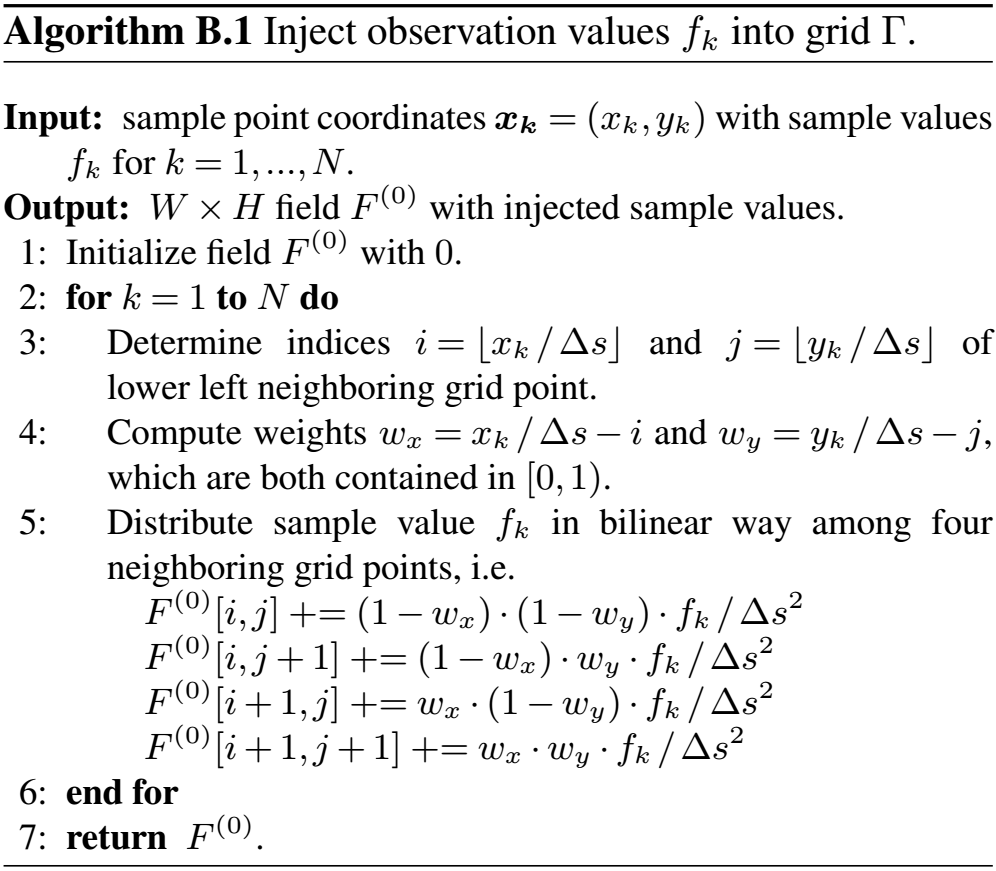
Note that if a grid point [i,j] is affected by several sample points, the determined weight fractions are accumulated accordingly in the respective field element F(0)[i,j]. For the final calculation of quotient (9), the factor cancels out and can therefore be omitted in Algorithm B.1, but for reasons of mathematical correctness, it is shown here. Since we have N input points and we perform a fixed number of operations for each of them, the complexity of Algorithm B.1 is given by 𝒪(N).
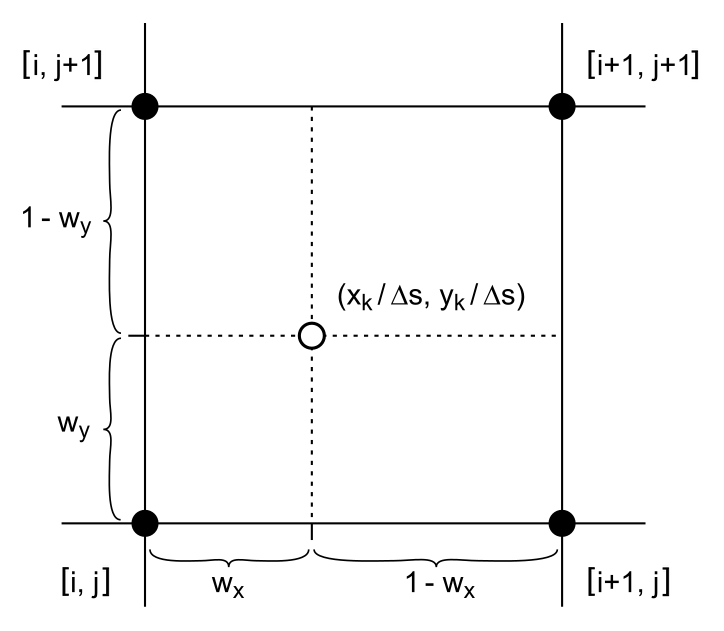
Figure 2The nearer a sample point xk is located to a grid point, the larger the weight assigned to it. Grid point [i,j], e.g., receives a weight of .
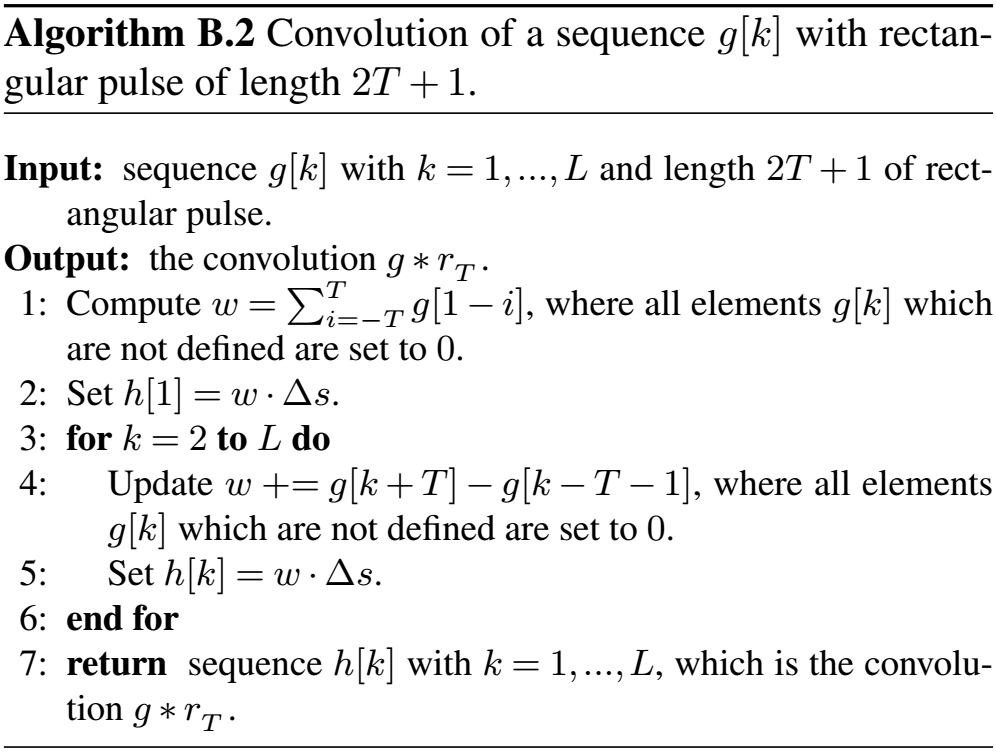
The other algorithmic fragment we require, which is implemented by Algorithm B.2, is the computation of a one-dimensional convolution of an arbitrary function g(x) with the rectangular function rn(x) as defined in Eq. (5). Employing the definition of convolution, we obtain
where . In other words, the convolution g ∗ rn at point x is simply the integral of g(x) in the window . Transferred to a one-dimensional grid with spacing Δs, the rectangular function rn(x) reads as rectangular pulse:
with a width parameter T∈ℕ0 that is gained by rounding to the nearest integer number:
Then, Eq. (10) translates in the discrete case to
where element h[k] corresponds to h(k⋅Δs) and g[i] to g(i⋅Δs). Equivalently to the continuous case, the value h[k] results up to a factor Δs from putting a window of length 2T+1 centrally over the sequence element g[k] and summing up all elements covered by it.
Assuming that we already computed h[k−1], it is immediately clear that the following value h[k] results from moving the window by one position to the right and thus can be obtained very easily from h[k−1] by adding the newly enclosed sequence element g[k+T] but subtracting element that falls outside the window.
As in the earlier case of Algorithm B.1, the factor Δs cancels out in the final calculation of Eq. (9) and can therefore also be omitted here.
Thus, Algorithm B.2 has 2T additions in step 1 and another 2(L−1) additions in the loop of step 3. Assuming that T is much smaller than L, an algorithmic complexity of 𝒪(L) results.
Now we are able to formulate Algorithm B.3 that computes convolutional expressions as found in the numerator and denominator of Approximation 3.
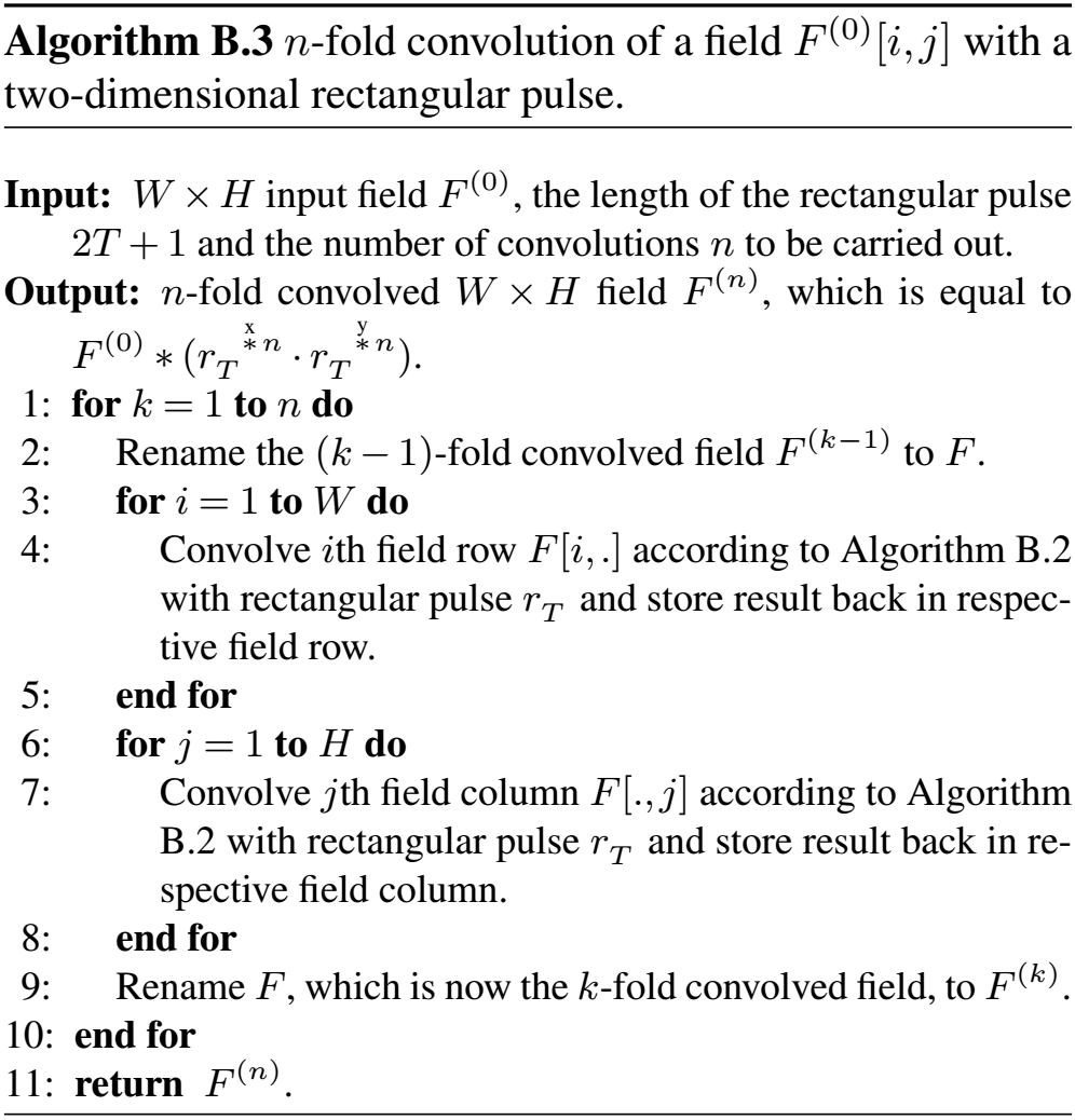
Note that due to the commutativity of and , the outer loop over index k can be moved inward within the loops over the rows and the columns, respectively. With this alternate loop layout, the field is first traversed row-wise in a single pass, where each row is convolved n times with rT in one sweep. Subsequently, the field is traversed column-wise and each column is convolved n times. In such a way, more economic strategies with respect to memory access can be achieved and moreover, this loop order is very well suited for parallel execution, such that Algorithm B.3 can be computed very efficiently. Since in practice n is chosen constant (proven values for n lie between 3 and 6), the algorithmic complexity is 𝒪(W⋅H).
Algorithms B.1 and B.3 now allow us to state the final Algorithm B, which implements the approximate computation of Barnes interpolation Eq. (9).
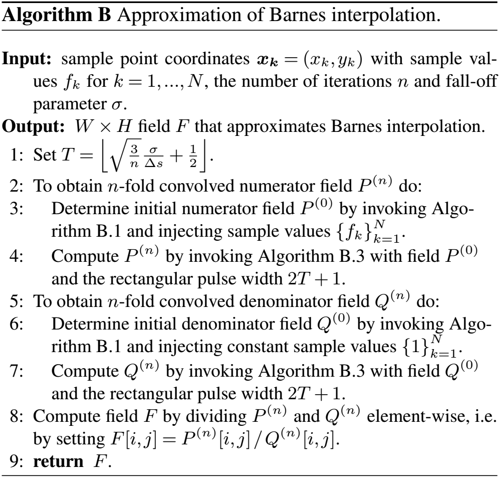
If the denominator Q(n)[i,j] in step 8 is 0, which is the case if the grid point [i,j] has a greater distance than 2nT from the nearest sample point in at least one dimension, the corresponding field value F[i,j] is undefined and set to NaN.
Since Algorithms B.1 and B.3 are invoked twice and step 8 employs another W⋅H divisions, the overall algorithmic complexity of the presented approach is limited to , which is a drastic improvement compared to the costs of of the naive implementation.
5.1 Test setup
The described Algorithm B – hereinafter denoted with “convolution” – was tested on a dataset that contained a total of 3490 QFF values (air pressure reduced to mean sea level) obtained from measurements at meteorological stations distributed over Europe and dating from the 27 July 2020 at 12:00 UTC. More specifically, we considered the geographic area ∘ E, 49∘ E]×[34.5∘ N, 72∘ N]⊂ℝ2, equipped with the Euclidean distance function defined on D×D, i.e., we measured distances in a first examination directly in the plate carrée projection neglecting the curved shape of the earth. The values of the QFF data range from 992.1 to 1023.2 hPa.
The convolution interpolation algorithm is subsequently compared with the results of two alternate algorithms. The first of them – referred to as “naive” – is given by the naive Algorithm A as stated in the Introduction. The second one – denoted with “radius” – consists of the improved naive algorithm that considers in its innermost loop only those observation points whose Gaussian weights w exceed 0.001 and thus are located within a radius of 3.717σ around the interpolation point. For this purpose, the implementation performs a so-called radius search on a k–d tree, which contains all observation points. Such a radius search can be achieved with a worst-case complexity of .
All algorithms were implemented in Python using the Numba just-in-time compiler (Lam et al., 2015) in order to achieve compiled code performance using ordinary Python code. The tests were conducted on a computer with a customary 2.6 GHz Intel i7-6600U processor with two cores, which is in fact only of minor importance since the tested code was written in single-threaded manner. All time measurements were performed 10 times and the best value among them was set as the final execution time of the respective algorithm.
5.2 Visual results
In general, the Barnes method yields a remarkably good interpolation and results in an aesthetic illustration for regions where the distance between the sample points has the same order of magnitude as the used Gaussian width parameter σ. However, if the distance between adjacent sample points is large compared to σ, this method exhibits some shortcomings because then the interpolation converges towards a step function with steep transitions. This effect can be clearly identified, for example, in the generation of plateaus of almost constant value over the Atlantic Ocean in Fig. 3a. In the limit case, if σ→0, the interpolation produces a Voronoi tessellation with cells of constant value around a sample point that are bordered by discontinuities towards the neighboring cells.
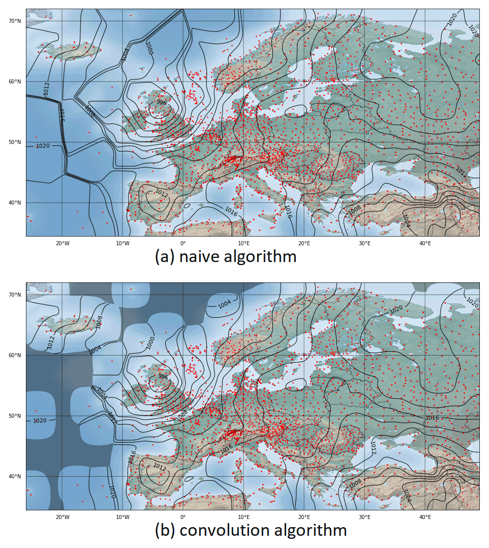
Figure 3Panel (a) shows exact Barnes interpolation with the naive algorithm for 3490 sample points depicted in red, a 2400×1200 grid with a resolution of 32 grid points per degree and . Panel (b) shows approximate Barnes interpolation with the convolution algorithm for the same settings as for the naive algorithm above. The applied 4-fold convolution uses a rectangular mask of size 57. Areas where the denominator of Eq. (9) drops below a value of 0.001 or is even 0 are rendered with a darker shade.
The comparison of the isoline visualizations in Fig. 3a and b shows an excellent agreement between the two approaches in the well-defined areas. The result for the radius algorithm is consistently similar to the other two and is therefore not depicted.
Note that the shaded, i.e., the undefined areas of Fig. 3b correspond to those areas where Barnes interpolation produces the plateau effect. In this sense, one can state that the convolution algorithm filters out the problematic areas in an inherent way.
5.3 Time measurements
For a grid of constant size, the measured execution times in Table 1 show a linear dependence to the number N of considered sample points for the naive and the radius algorithms, while they are almost constant for the presented convolution algorithm. The costs of the injection step are obviously more or less inexistent compared to the costs of the subsequent steps of the algorithm. This fact is in total agreement with the deduced complexity , since in our test setup, the grid size W×H clearly dominates over N.
Table 1Execution times (in s) of the investigated algorithms for varying numbers of sample points. The grid size of 2400×1200 points with a resolution of 32 points per degree and the Gaussian width are kept constant. The convolution algorithm applied a 4-fold convolution.
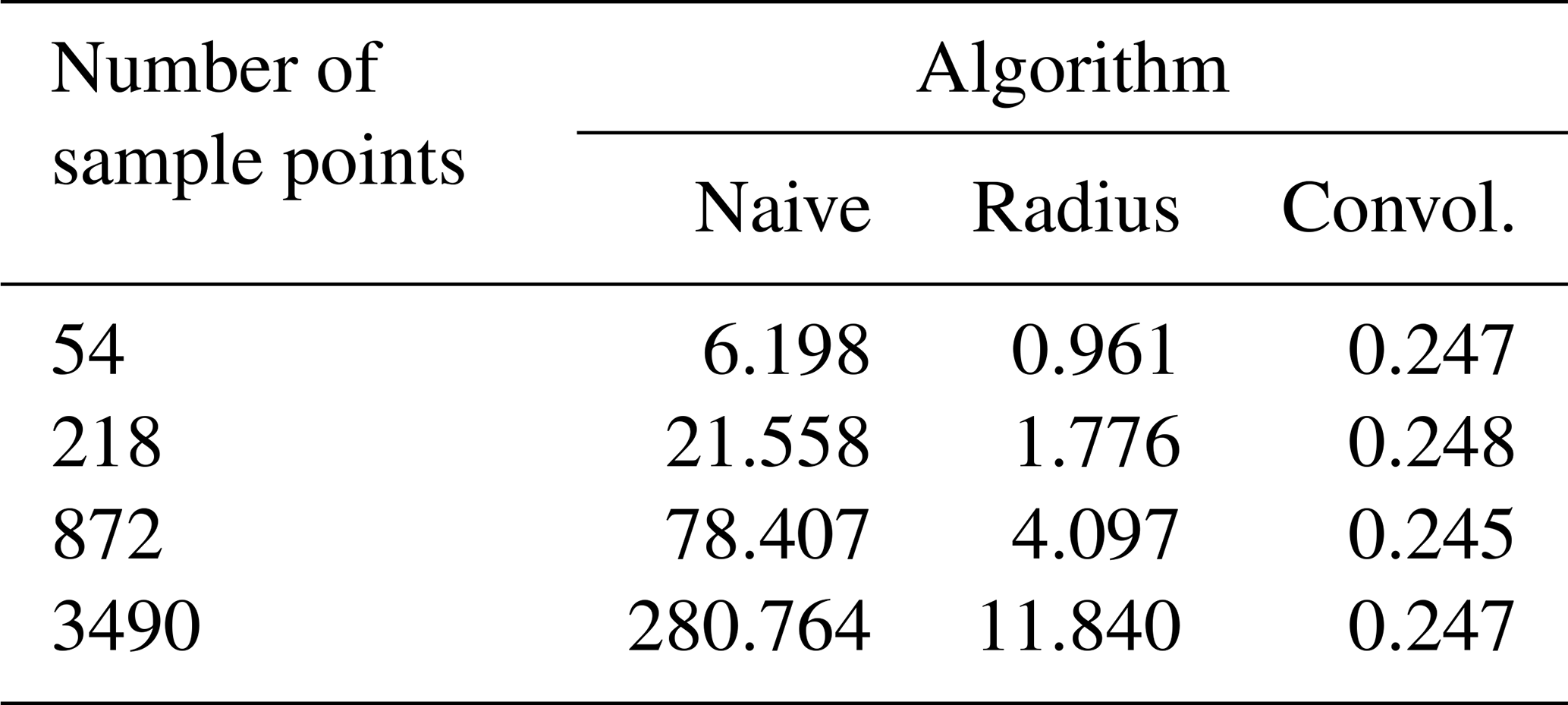
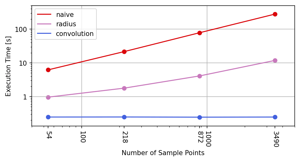
Figure 4Plot of execution times from Table 1 against number of sample points. Both axes use a logarithmic scale.
Also note that between the naive and the convolution algorithms, the speed-up factor roughly ranges between 25 and 1000 for the considered number of sample points.
If the grid size is varied, all considered algorithms reveal a linear-like dependence to the number of points in the grid as can be seen in Table 2 and Fig. 5. For smaller grid sizes, the convolution algorithm provides a speed-up factor of around 2000 compared to the naive implementation, but for bigger grids, the factor drops below 1000.
This effect can be explained by the fact that the crucial parts of the convolution algorithm access memory for smaller grids with a high spatial and temporal locality and thus make optimal use of the highly efficient CPU cache memory (Patterson and Hennessy, 2014). For bigger grids, the number of cache misses increases, which result in a slightly degraded performance.
Table 2Execution times (in s) of the investigated algorithms for varying grid sizes and resolutions, respectively. The number of sample points N=3490 and the Gaussian width are kept constant. The convolution algorithm applied a 4-fold convolution.
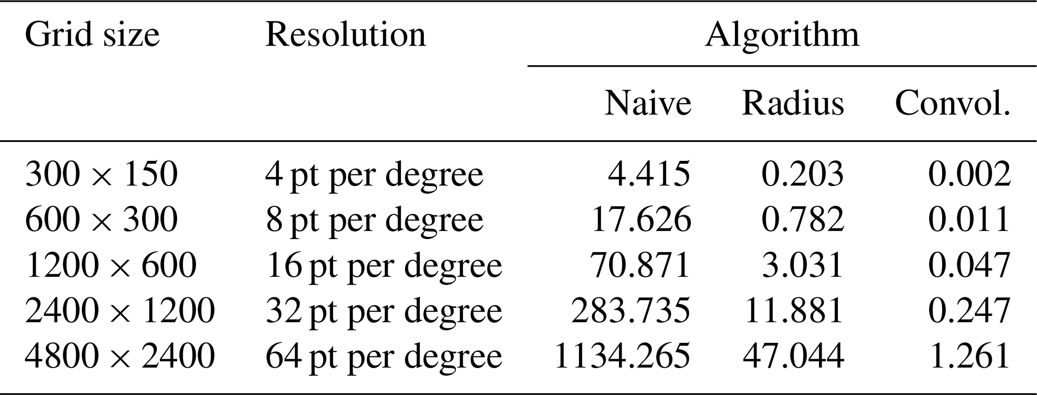
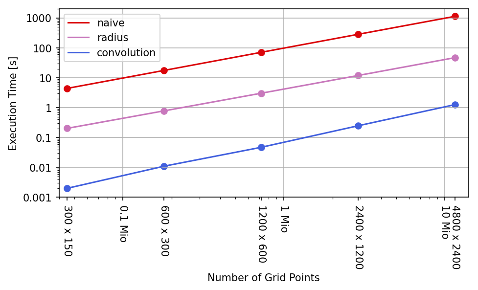
Figure 5Plot of execution times from Table 2 against number of grid points. Both axes use a logarithmic scale.
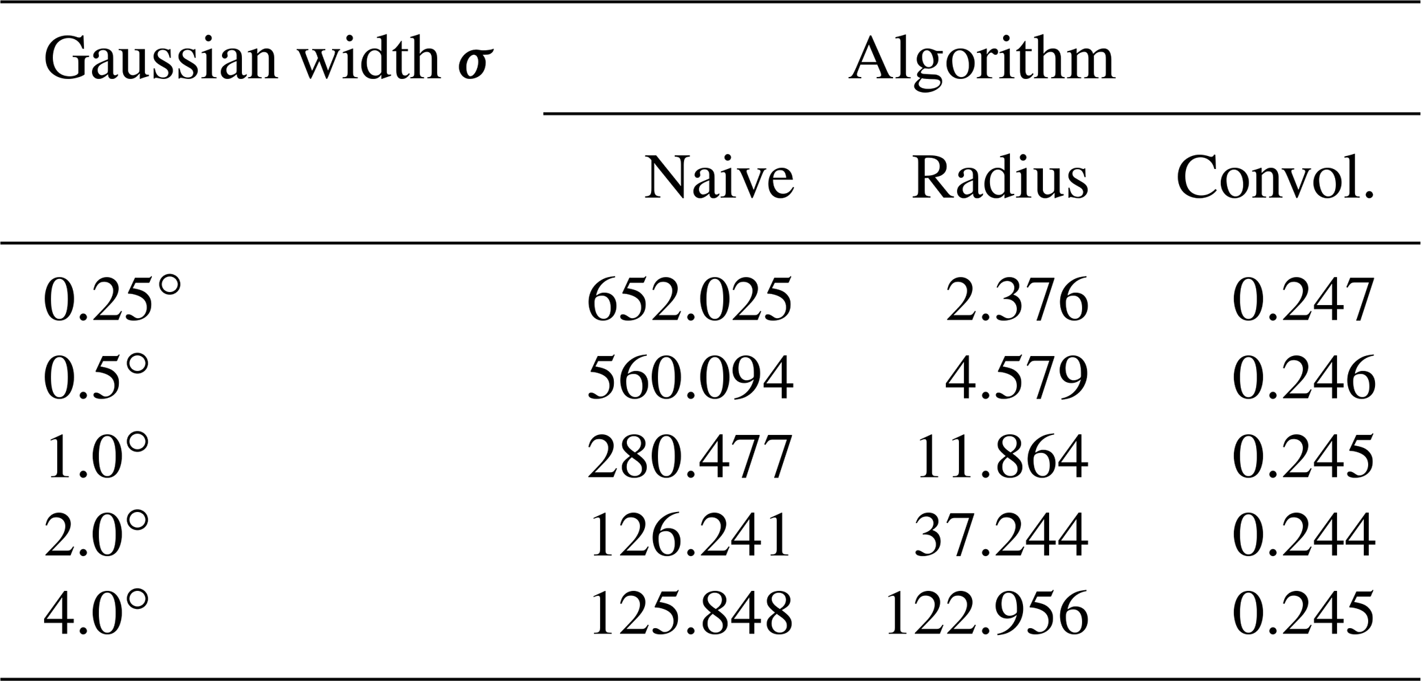
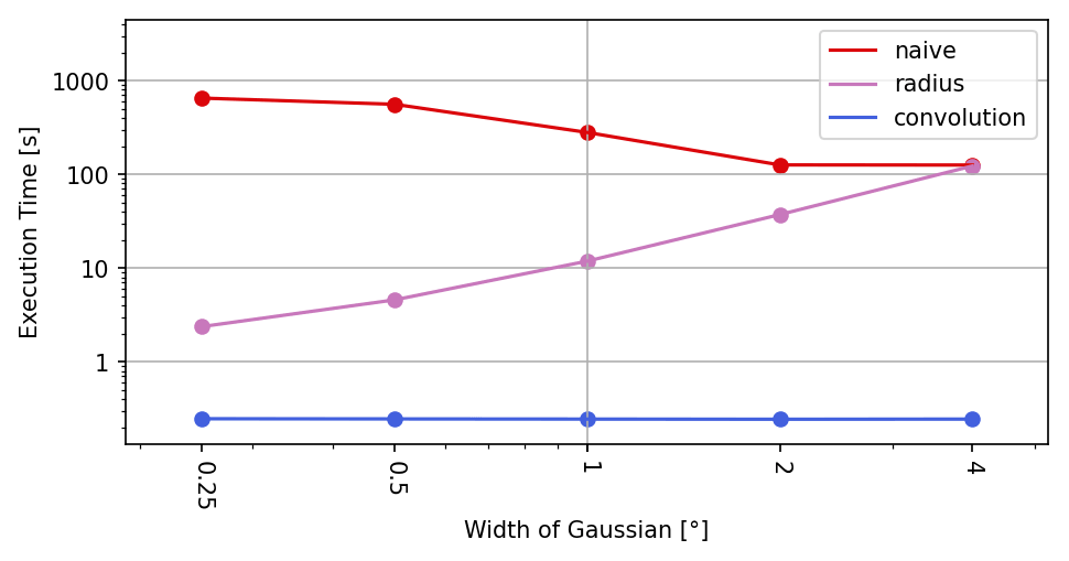
As is to be expected, the Gaussian width parameter σ has no decisive impact on the execution times measured for the naive and the convolution algorithms (refer to Table 3 and Fig. 6). The radius algorithm, on the other hand, shows a quadratic dependence, since the relevant area around a grid point – and thus also the average number of sample points to be considered – grows quadratically with the radius of influence, which in turn depends linearly on σ.
The unstable time measurements for the naive algorithm are caused by a peculiar execution time behavior of the exponential function. Although the value of Eq. (2) is less than the smallest representable float and therefore results in 0 for distances d>38.6σ, its computational cost increases to a multiple of the time needed for shorter distances. With growing σ, this computational overhead is less and less noticeable in the test series.
Table 3Execution times (in s) of the investigated algorithms for varying Gaussian width parameters σ. The number of sample points N=3490 and the grid size of 2400×1200 points with a resolution of 32 points per degree are kept constant. The convolution algorithm applied a 4-fold convolution.
5.4 Algorithm fine tuning
In the discretization step, we round off the window width parameter T∈ℕ0 to the nearest integer, i.e., we set
and then repeatedly convolve the input fields with a rectangular pulse signal rT[k] that has a length 2T+1. In the extreme case, if n exceeds and hence T=0, the underlying pulse signal degrades to r0[k], which is identical to the discrete unit pulse, the neutral element with respect to convolution. Under these circumstances, the algorithm stops rendering a meaningful interpolation. Since normally σ>Δs, the respective bound for n can go into the hundreds, which is why the described extreme case is typically not encountered for real applications.
Nevertheless, a general consequence of the rounding operation is that the effectively obtained Gaussian width σeff for our algorithm only approximates the desired width σ. For the following considerations, let uT[k] be the uniform probability distribution that corresponds to rT[k], i.e.,
By algorithmic design, is the variance of uT[k], which is convolved n times with itself and which is employed on a grid with point spacing Δs. Therefore,
For T≥1, the integer number T can be fixed by Eq. (11) to the unit interval
which in turn allows us to derive sharp bounds for σeff when substituted into Eq. (12):
The last relation reveals that the range of possible values for σeff grows with increasing n until σeff collapses to 0 when , as we have seen further above. In summary, there are two diametrically opposed effects that determine the result quality of the presented algorithm. From the perspective of the central limit theorem, the approximation performance is better for large n, while on the other hand, σeff tends to be closer to the target σ for small n.
If full accuracy is required for the Gaussian width and the grid spacing Δs is not strictly given in advance, one can tune the spacing such that the resulting width σeff corresponds exactly to the desired σ. For T≥1, Eq. (12) then allows us to determine the necessary grid step as
If, however, the grid is fixed a priori and cannot be modified, the only option to attain the requested σ exactly is to refrain from using a stringent rectangular pulse and to employ a slightly more complicated signal (Gwosdek et al., 2011). For this purpose, we set this time as follows:
which is gained from taking the positive solution of the quadratic Eq. (12) for T. Now we have and we define the linearly blended signal for :
This modified signal rT,α[k] is basically the pure rectangular signal rT[k] of unit elements with a trailing element α appended at both ends. Due to the continuity of the variance, there must be a specific for which , whereas designates the probability distribution of rT,α[k]. With
we conclude that the wanted is given by
The respective expression for derived in (Gwosdek et al., 2011) corresponds to a special case of Eq. (14) when setting Δs=1.
Remember now that the central limit theorem is valid for any PDF, which means that the mathematical framework presented in the previous chapters is also valid for the modified signal . Therefore, we receive an optimized approximate Barnes interpolation by marginally adapting Algorithm B.2 to compute the convolution with instead of rT[k]. To do so, steps 2 and 5 of it have to be rewritten to . Although the optimized approach requires 2L additions and L multiplications more than the original one, the adapted Algorithm B.2 remains in the complexity class 𝒪(L). Measurements (refer to Table 4 and Fig. 7) show that the optimized interpolation in fact needs only about 10 % to 30 % more time for the depicted range of convolution rounds than the original one.
Table 4Signal width parameter T and the effective Gaussian width σeff for the original convolution algorithm and the tail value for the optimized convolution algorithm as a function of the number of performed convolutions n, where N=3490, grid size is 2400×1200, with a resolution of 32 points per degree and . The root mean square error RMSE is computed for the sub-area displayed in Fig. 9 and with respect to the exact results of the naive algorithm. The execution times texec are measured in seconds.
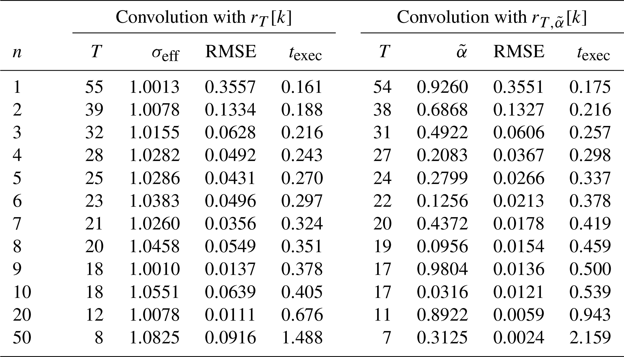
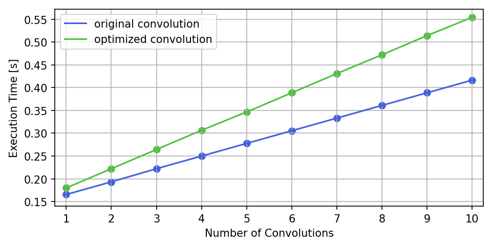
Figure 7Plot of execution times from Table 4 against number of performed convolutions for both the original and the optimized convolution algorithms.
The unstable behavior of the original convolution algorithm with respect to the number of performed convolutions can be best observed in the RMSE plot of Fig. 8, where the baseline is given by the exact interpolation of the naive algorithm. A corresponding unsteady feature is also visible in the upper row of the maps shown in Fig. 9a, more precisely in the fluctuating diameter of the small high-pressure area west of the Balearic Islands.
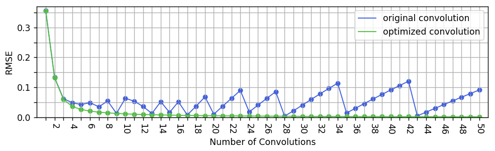
Figure 8Root mean square error with respect to the exact Barnes interpolation in dependency of the number of performed convolutions for both the original and the optimized convolution algorithms.
In contrast to that, the optimal convolution algorithm shows a stable convergence towards the exact interpolation obtained by the naive algorithm, which manifests in strictly monotonic decreasing RMSE values. These results suggest that three or four performed convolution rounds already achieve a very good approximation of Barnes interpolation when used to visualize data, as done in this paper. For other applications, which require a higher precision, a 10-fold convolution or even more might make sense.
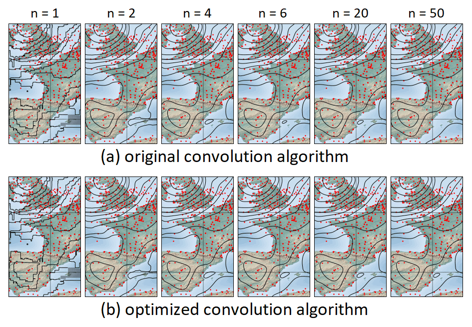
Figure 9Results for a different number of performed convolutions n. Upper row (a) with results for the original convolution algorithm and lower row (b) with results for the optimized convolution algorithm.
5.5 Application on sphere geometry
So far, we applied the convolution algorithm on sample points contained in the plane ℝ2 and used the Euclidean distance measure. For geospatial applications, this simplification is acceptable as long as the considered area is sufficiently small enough. If we deal with a dataset, which is distributed over a larger region – as it is actually the case in our test setup – it becomes necessary to take the curvature of the earth into account.
The adaptation of the naive Barnes interpolation algorithm to the spherical geometry on 𝒮2 merely comprises the exchange of the Euclidean distance with the spherical distance. Since the calculation of the spherical distance between two points involves several trigonometric function calls, the price of such a switchover is accordingly high and consequently, the exact Barnes interpolation for a spherical geometry is roughly a factor of 2.5 times slower in our tests than that with the Euclidean approach. In other words, an already costly algorithm becomes even more expensive.
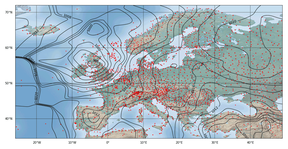
Figure 10Exact Barnes interpolation with the naive algorithm for the same setup as for Fig. 3 but using spherical distances from 𝒮2 instead of Euclidean distances from ℝ2. The generated isolines are notably different in the northern part, while they are quite similar in the south.
However, the distance calculation does not occur explicitly in the convolution algorithm, since the latter by virtue of the central limit theorem is inherently tied to the Euclidean distance measure. Therefore, the convolution algorithm has to be transferred to the spherical geometry with a different method.
The chosen approach is to first map the sample points to a map projection, which distorts the region of interest as minimal as possible and then to apply the convolution algorithm directly in that map space. The resulting field is finally mapped back to the original map projection and provides an approximation of Barnes interpolation there with respect to the spherical geometry of 𝒮2.
Projection types that are considered suitable for this purpose are conformal map projections. Conformal maps preserve angles and shapes locally, while distances and areas underlie a certain distortion. Conformal maps used often are (Snyder, 1987)
-
Mercator projection for regions of interest that stretch in east–west direction around the Equator,
-
transverse Mercator projection for regions with north–south orientation,
-
Lambert conformal conic projection for regions in the mid-latitudes that stretch in east–west direction or
-
polar stereographic projection for polar regions.
In order to replicate Fig. 10 with our fast optimized convolution algorithm, we therefore use a Lambert conformal conic map projection for our test setup with sample points in the mid-latitudes. We choose the two standard parallels that define the exact projection at latitudes of 42.5 and 65.5∘ N, such that our region of interest is evenly captured by them. By nature of Lambert conformal conic maps, the chosen map scale is exactly adopted along these two latitudes, while it is too small between them and too large beyond them. Similarly, for a grid with a formal resolution of 32 grid points per degree that is embedded into this map, the specified resolution only applies exactly along the standard parallels, while the effective resolution between them is smaller and larger beyond them.
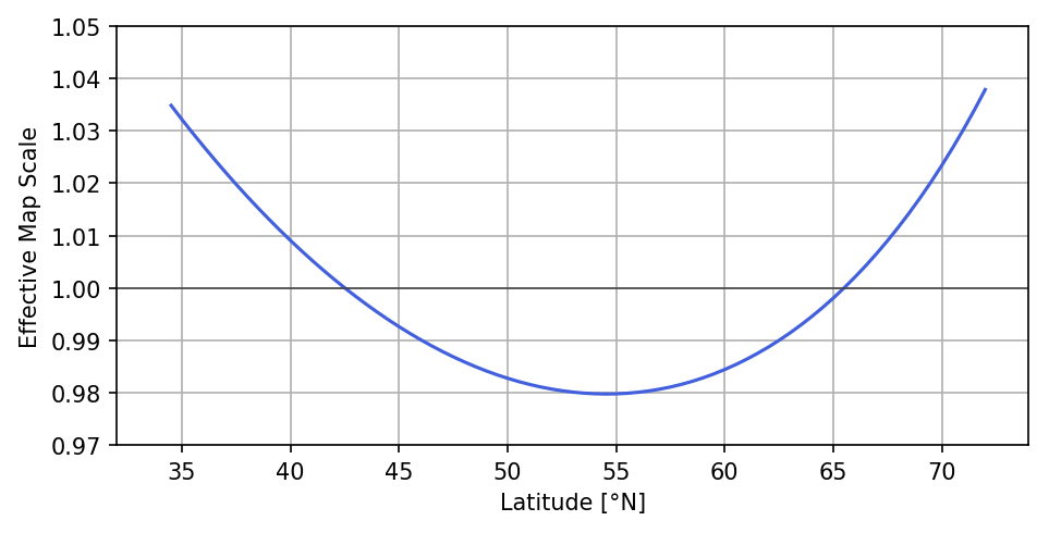
Figure 11The effective scale of a Lambert conformal conic map in dependency of the latitude if the scale at 42.5 and 65.5∘ N is set to 1.0. The minimum scale of 0.98 is reached at a latitude of 54.5∘ N.
We now employ the optimized convolution algorithm with a nominal Gaussian width parameter on the Lambert conformal conic map grid postulated above, in which we injected the given sample points beforehand. The resulting field shown in Fig. 12 thereby experiences a 2-fold approximation, the first one caused by the distortion of the map and the second one due to the approximation property of the convolution algorithm.
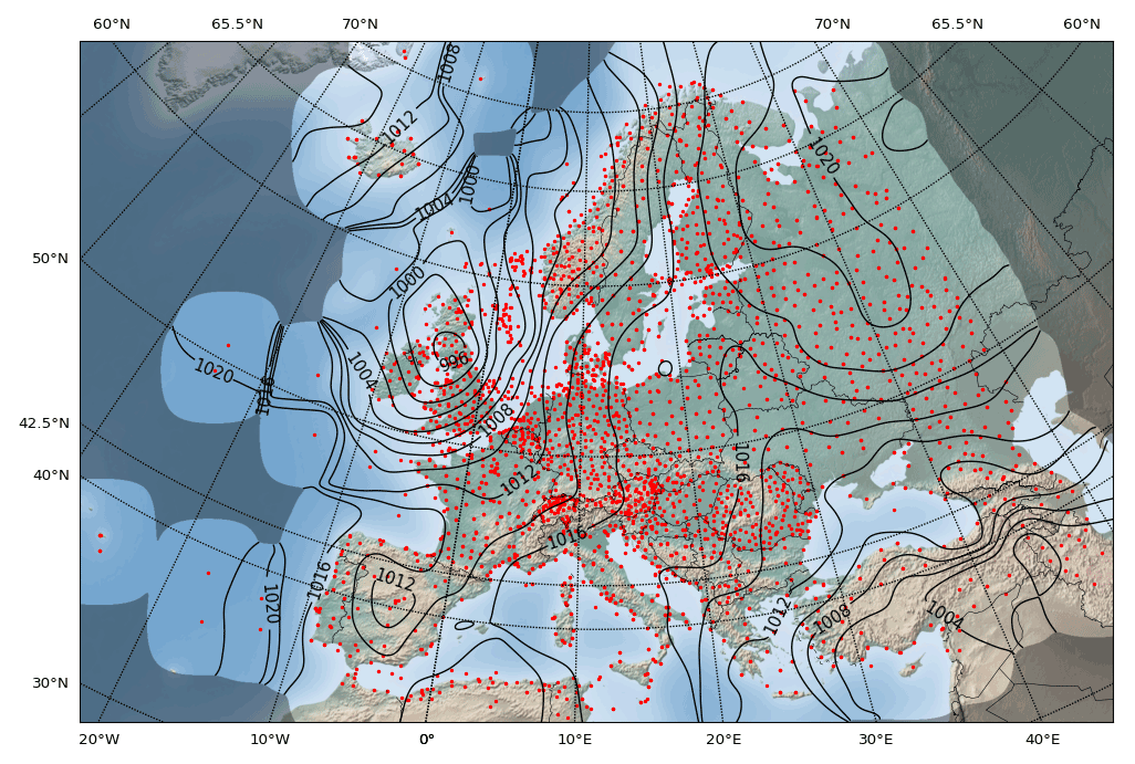
Figure 12Optimized Barnes interpolation algorithm applied on the Lambert conformal map on a 2048×1408 grid with a resolution of 32 grid points per degree along the standard parallels at 42.5 and 65.5∘ N, and a 4-fold convolution.
In a last step, the result field is mapped back to the target map, which uses a plate carrée projection in our case. In order to do this, the location of a target field element is looked up in the Lambert map source field and subsequently its element value is determined by bilinear interpolation of the four neighboring source field element values. This last operation performs an averaging and thus adds a further small error to the final result shown in Fig. 13. Similar to the case for the Euclidean distance, the comparison with the exact Barnes interpolation on 𝒮2 in Fig. 10 yields a very good correspondence. This perception is also supported by measurement of the RMSE, which adds up for the same sub-area as investigated in Table 4 to 0.0467, which is negligibly larger than the corresponding 0.0367 measured for the Euclidean case.
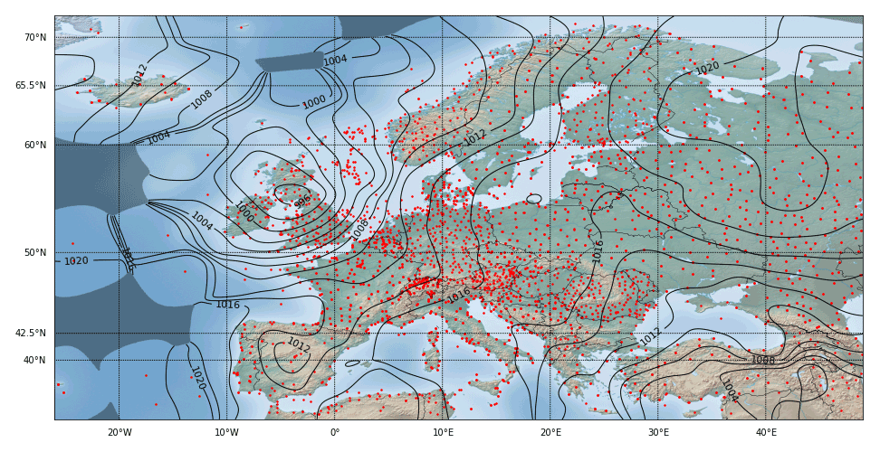
Figure 13Resulting field from Fig. 12 projected back to a plate carrée map.
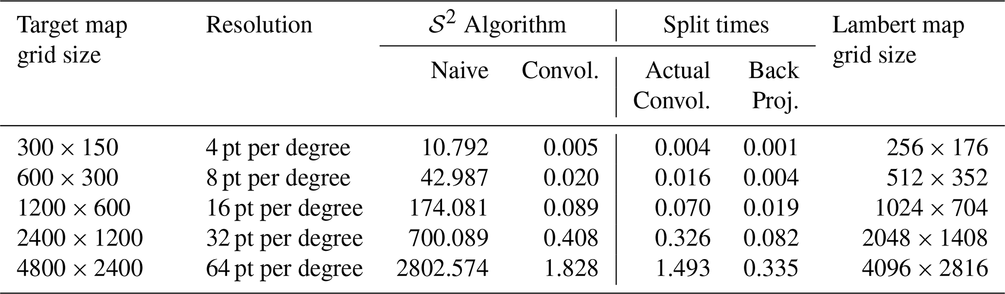
Table 5Execution times (in s) for the naive and the optimized convolution algorithms using spherical distances on 𝒮2 for varying grid sizes. The number of sample points N=3490 and the Gaussian width are kept constant. The convolution algorithm applied a 4-fold convolution and was executed on a Lambert map grid of the indicated size. The two split time columns show the separated execution times for the actual convolution and the subsequent back projection to the plate carrée map. For the investigated scenarios, the optimized convolution algorithm is more than 1000 times faster than the naive one.
5.6 Round-off error issues
Computing the convolution of a rectangular pulse in floating-point arithmetic using the moving window technique as described in Algorithm B.2 of Sect. 4 is extremely efficient, but it is also prone to imprecisions since round-off errors are steadily accumulated during the progress. Different approaches are known to reduce this error. The Kahan summation algorithm (Kahan, 1965), for instance, implements an error-compensation scheme at the expense of requiring essentially more basic operations than used for ordinary addition.
Another error-reduction technique that is effective in the context of Barnes interpolation is to center the numbers to be added around 0.0, where the mesh density of representable floating-point numbers is highest. For this purpose, an offset
is initially subtracted from the sample values fk, such that their range is exactly located around 0.0. The presented convolution algorithm is then applied to the shifted sample values. In a final step, the elements of the resulting field F[i,j] are shifted back to the original range by adding to each of them. This modification basically needs extra additions, such that the computational complexity of the convolution algorithm is not harmed and stays unchanged.
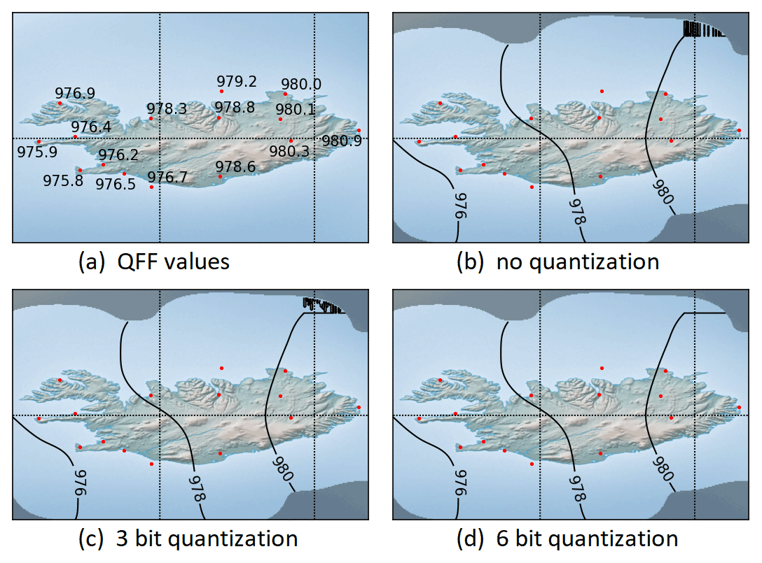
Figure 14Constellation of QFF values over Iceland with generated isolines for . Note the 980.0 hPa observation value in the northeast of Iceland, which triggers the creation of the faulty isoline for the same value. By increasing the quantization degree of the resulting field values, the visual appearance is gradually improved.
Minimal numerical round-off errors can generate surprisingly prominent artifacts when areas of constant or near-constant data are rendered with an isoline visualization. In such cases, the value obtained by the convolution algorithm fluctuates seemingly randomly around the true constant value, and if it happens that one of the rendered isolines represents exactly this value, the visualized result may appear like a fractal curve as shown in Fig. 14. A counter measure against this effect is to apply a quantization scheme to the resulting values, which basically suppresses a suitable number of least significant bits and rounds the value off to the nearest eligible floating point number. After this operation, the obtained values in areas of constant data are actually constant and thus result in a more pleasant isoline visualization. In areas with varying data values, the quantization of the result data has no harmful impact.
We presented a new technique for computing very good approximations of Barnes interpolation, which offers speed-up factors for realistic scenarios that can reach into the hundreds or even into the thousands when applied on a spherical geometry. The underlying convolutional algorithm exhibits a computational complexity of , in which the number of sample points N is decoupled from the grid size W×H. This is a major improvement over the computational complexity of the naive algorithm of . Our tests suggest that four to six iteration rounds of convolutions lead to approximations of Barnes interpolation that achieve highly satisfactory results for most applications.
The usage of the algorithm is not restricted to ℝ2 or 𝒮2 and it can easily be extended to higher dimensional spaces ℝn. The algorithm allows us to incorporate quality measures that assign each sample point xk a weight of certainty ck, which specifies how much this point shall contribute to the overall result. To achieve this, the terms in the two sums in Eq. (1) are simply multiplied by the additional factor ck, and likewise the same factors then also appear in Approximation 3.
Barnes interpolation is often used in the context of successive correction methods (Cressman, 1959; Bratseth, 1986) with or without a first guess from a background field. In this technique, the interpolation is not performed just once, but applied several times with decreasing Gaussian width parameters to the residual errors in order to minimize them successively. Needless to say that instead of exact Barnes interpolation, the convolutional algorithm can equally be used for the method of successive correction.
Since the presented solution for spherical geometries is only suitable for the treatment of local maps, we plan to generalize the approach to global maps in a next step. This could for instance be done by smoothly merging local Barnes interpolation approximation patches into a global approximation.
Furthermore, we also want to provide a statement about the quality of the calculated approximation depending on the number of performed convolutions by deriving a theoretical upper bound for the maximum possible error. It will also be of interest, in a similar way to Getreuer (2013), to consider other distributions for the approximation and investigate their behavior in terms of computational speed and accuracy.
For an integrable function , the n-fold convolution with itself f∗n(x) is recursively defined by
with . The equivalent closed form representation
is in most cases only of formal interest, since in practice the effective calculation of the multiple integral will lead to the recursive definition (A1) again.
Analogously, in the case of an integrable function of two variables , the n-fold convolution with itself is recursively given by
for and with .
A function of two variables is called separable if two functions of one variable g1(x) and g2(y) exist, both in L1(ℝ), such that the following equality holds:
The convolution of f(x,y) with a separable function can be decomposed into two unidirectional convolutions that only act along one of the coordinate axis. In order to make this clear, we define two left-associative operators and that map from by setting
where convolves along the x axis and along the y axis. With these definitions, we then find
From the fact that we can change the order of integration, we finally infer the following:
Hence, the two operands g1 and g2 commute, but note here that the unidirectional operators to their left have to be swapped with them as well. The n-fold convolution with a separable function thus decomposes into
Due to the commutation law (B4), we can basically write the operands on the RHS of f in any order, but we prefer to group them as
Because the last formula looks a bit cumbersome, we again use Eq. (B4) to join the two n-fold self-convoluted operands to a separable function, which then reads as
Throughout the paper, we use the concise representation of Eq. (B6) but keep in mind that it is equivalent to Eq. (B5), where each convolution operand is expressed separately, and thus indicates clearly how this expression is to be calculated.
For the derivation of Approximation 3, we used a separable two-dimensional PDF that consists of two uniform one-dimensional distributions.
This result can be broadened, if more general marginal distributions are employed.
For this purpose, let p1(x) and p2(x) be two one-dimensional PDFs with mean 0 and variance .
Now, we define the separable two-dimensional PDF , which has a mean vector 0 and a covariance matrix .
Consequently, the PDF p(x,y) constructed in this way satisfies the assumptions of the central limit theorem (6) and thus, after performing the same conversion steps as taken in Sect. 3, follows the generalized
Approximation 4. For sufficiently large n, Barnes interpolation on the Euclidean plane ℝ2 can be approximated by
provided that the quotient is defined.
In practice, p1(x) and p2(x) will most often be chosen to be identical. Using the normal distribution φ0,σ(x) with mean value 0 and variance σ2, i.e.,
it is clear from Eq. (8) that we can formulate Barnes interpolation based on a convolutional expression where even equality holds.
Let φ0,σ(x) be the normal distribution with mean value 0 and variance σ2. For Barnes interpolation on the Euclidean plane ℝ2, the following then holds:
Note that in the case of the normal distribution, it is sufficient to apply the convolution just once.
The formal algorithms introduced in this paper are provided as Python implementation on GitHub https://github.com/MeteoSwiss/fast-barnes-py (last access: 11 March 2023) under the terms of the BSD 3-clause license and are archived on Zenodo https://doi.org/10.5281/zenodo.7651530 (Zürcher, 2023a). The sample dataset and the scripts are also included, which allow us to reproduce the figures and tables presented in this paper. The interpolation code is available as well as Python package fast-barnes-py on https://PyPI.org/project/fast-barnes-py (Zürcher, 2023b).
The author has declared that there are no competing interests.
Publisher's note: Copernicus Publications remains neutral with regard to jurisdictional claims in published maps and institutional affiliations.
The author would like to thank the topical editor Sylwester Arabas and the two anonymous reviewers for their valuable comments and helpful suggestions. All map backgrounds were made with Natural Earth, which provides free vector and raster map data at https://naturalearthdata.com (last access: 11 March 2023).
This paper was edited by Sylwester Arabas and reviewed by two anonymous referees.
Barnes, S. L.: A Technique for Maximizing Details in Numerical Weather Map Analysis, J. Appl. Meteorol., 3, 396–409, https://doi.org/10.1175/1520-0450(1964)003<0396:ATFMDI>2.0.CO;2, 1964. a
Bentley, J. L.: Multidimensional Binary Search Trees Used for Associative Searching, Commun. ACM, 18, 509–517, https://doi.org/10.1145/361002.361007, 1975. a
Bratseth, A. M.: Statistical interpolation by means of successive corrections, Tellus A, 38, 439–447, https://doi.org/10.3402/tellusa.v38i5.11730, 1986. a
Cressman, G. P.: An Operational Objective Analysis System, Mon. Weather Rev., 87, 367–374, https://doi.org/10.1175/1520-0493(1959)087<0367:AOOAS>2.0.CO;2, 1959. a
Daley, R.: Atmospheric Data Analysis, Cambridge University Press, Cambridge, https://doi.org/10.1002/joc.3370120708, 1991. a
Finkel, R. A. and Bentley, J. L.: Quad Trees, a Data Structure for Retrieval on Composite Keys, Acta Inform., 4, 1–9, https://doi.org/10.1007/BF00288933, 1974. a
Getreuer, P.: A Survey of Gaussian Convolution Algorithms, Image Processing On Line, 3, 286–310, https://doi.org/10.5201/ipol.2013.87, 2013. a
Gwosdek, P., Grewenig, S., Bruhn, A., and Weickert, J.: Theoretical foundations of Gaussian convolution by extended box filtering, International Conference on Scale Space and Variational Methods in Computer Vision, 447–458, https://doi.org/10.1007/978-3-642-24785-9_38, 2011. a, b
Kahan, W.: Further remarks on reducing truncation errors, Commun. ACM, 8, 40, https://doi.org/10.1145/363707.363723, 1965. a
Klenke, A.: Probability Theory: a Comprehensive Course, 3rd Edn., Universitext, Springer, https://doi.org/10.1007/978-3-030-56402-5, 2020. a, b
Koppert, H. J., Pedersen, T. S., Zürcher, B., and Joe, P.: How to make an international meteorological workstation project successful, Twentieth International Conference on Interactive Information and Processing Systems for Meteorology, Oceanography, and Hydrology, 84th AMS Annual Meeting, Seattle, WA, 11.1, https://ams.confex.com/ams/84Annual/techprogram/paper_71789.htm (last access: 11 March 2023), 2004. a
Lam, S. K., Pitrou, A., and Seibert, S.: Numba: A LLVM-based Python JIT Compiler, LLVM '15: Proceedings of the Second Workshop on the LLVM Compiler Infrastructure in HPC, 1–6, https://doi.org/10.1145/2833157.2833162, 2015. a
Muirhead, R. J.: Aspects of Multivariate Statistical Theory, Wiley Series in Probability and Mathematical Statistics, John Wiley & Sons, Inc., https://doi.org/10.1002/9780470316559, 1982. a
Patterson, D. A. and Hennessy, J. L.: Computer Organization and Design: the Hardware/Software Interface, 5th Edn., Elsevier, https://dl.acm.org/doi/book/10.5555/2568134 (last access: 11 March 2023), 2014. a
Snyder, J. P.: Map Projections: A Working Manual, US Geological Survey Professional Paper 1395, US Government Printing Office, Washington, https://doi.org/10.3133/pp1395, 1987. a
Wells, W. M.: Efficient Synthesis of Gaussian Filters by Cascaded Uniform Filters, IEEE T. Pattern Anal., 8, 2, 234–239, https://doi.org/10.1109/TPAMI.1986.4767776, 1986. a
Zürcher, B.: MeteoSwiss/fast-barnes-py: fast-barnes-py v1.0.0 (v1.0.0), Zenodo [code], https://doi.org/10.5281/zenodo.7651530, 2023a. a
Zürcher B.: fast-barnes-py 1.0.0, PyPI [code], https://PyPI.org/project/fast-barnes-py, last access: 11 March 2023b. a
- Abstract
- Introduction
- Conclusions from central limit theorem
- Barnes interpolation as series of convolutions
- Discretization
- Results and further considerations
- Summary and outlook
- Appendix A: n-fold self-convolution
- Appendix B: Separable functions
- Appendix C: Generalized approximate Barnes interpolation
- Code and data availability
- Competing interests
- Disclaimer
- Acknowledgements
- Review statement
- References