the Creative Commons Attribution 4.0 License.
the Creative Commons Attribution 4.0 License.
 | 17 Mar 2023
Evaluating a global soil moisture dataset from a multitask model (GSM3 v1.0) with potential applications for crop threats
Jiangtao Liu
David Hughes
Farshid Rahmani
Kathryn Lawson
Climate change threatens our ability to grow food for an ever-increasing population. There is a need for high-quality soil moisture predictions in under-monitored regions like Africa. However, it is unclear if soil moisture processes are globally similar enough to allow our models trained on available in situ data to maintain accuracy in unmonitored regions. We present a multitask long short-term memory (LSTM) model that learns simultaneously from global satellite-based data and in situ soil moisture data. This model is evaluated in both random spatial holdout mode and continental holdout mode (trained on some continents, tested on a different one). The model compared favorably to current land surface models, satellite products, and a candidate machine learning model, reaching a global median correlation of 0.792 for the random spatial holdout test. It behaved surprisingly well in Africa and Australia, showing high correlation even when we excluded their sites from the training set, but it performed relatively poorly in Alaska where rapid changes are occurring. In all but one continent (Asia), the multitask model in the worst-case scenario test performed better than the soil moisture active passive (SMAP) 9 km product. Factorial analysis has shown that the LSTM model's accuracy varies with terrain aspect, resulting in lower performance for dry and south-facing slopes or wet and north-facing slopes. This knowledge helps us apply the model while understanding its limitations. This model is being integrated into an operational agricultural assistance application which currently provides information to 13 million African farmers.
- Article
(5629 KB) - Full-text XML
-
Supplement
(627 KB) - BibTeX
- EndNote


Soil moisture is a critical variable that influences a number of natural disasters. As a result, widely available, high-quality soil moisture products can be vital for regions that need aid. Too much soil moisture can prime the landscape for floods (Norbiato et al., 2008), and too little of it for too long can damage or kill crops and native vegetation (Narasimhan and Srinivasan, 2005; Sheffield and Wood, 2008). Moreover, many insect pests lay eggs in soils with certain soil moisture conditions – for example, locusts prefer to lay their eggs in sandy, wet soils (Hunter-Jones, 1964). In the year 2020, disastrous locust swarms terrorized large swaths of eastern Africa and Southeast Asia (Baraniuk, 2020; UN WFP, 2020). The knowledge of soil moisture levels can be critical in planning pest control activities, as the immature stages are the best targets for effective control (Ellenburg et al., 2021; Nuwer, 2021). Besides insect pests, pathogenic fungi and bacteria can be heavily influenced by soil moisture, resulting in crop losses. In all of these cases, soil moisture products can be highly valuable in reducing both current and emerging threats to crops. Finally, the current global crisis in fertilizer availability following the ongoing war in Europe (Bentley et al., 2022) necessitates strategies that increase the efficient use of fertilizer, for which a precise understanding of soil moisture is critical because water availability in the soil affects both plant uptake of fertilizer and fertilizer loss.
Soil moisture is monitored globally by a number of satellite missions and is simulated globally by multiple land surface hydrologic models, but these products have their respective limitations. Satellite missions like Soil Moisture Active Passive (SMAP) (Entekhabi, 2010) and Soil Moisture and Ocean Salinity (SMOS) (Kerr et al., 2010) have limited spatial resolution and accuracy. When evaluated in comparison to in situ data, especially on sparsely instrumented sites that are outside of the missions' core calibration and validation sites, their error can be high (Al-Yaari et al., 2017) (also demonstrated later in this work). Land surface models can also produce decent simulations with seamless spatiotemporal coverage (Albergel et al., 2018; Beaudoing and Rodell, 2019; Yang et al., 2011), but they may not be fully exploiting available information, as evidenced by the better performance produced by machine learning models where data are available (Liu et al., 2022a; O and Orth, 2021). Both satellite and model products may also have a large bias compared to in situ data.
Recently, we developed a multiscale time series deep learning (DL) model that learns simultaneously from satellite and in situ data and can substantially outperform satellite-based products, a model trained on in situ data alone, and traditional land surface model simulations (Liu et al., 2022a). In a spatial cross-validation test (trained on some sites and tested on others), the multiscale DL model obtained a median correlation (R) of 0.901 when evaluated by the sparse soil moisture network over the conterminous United States (CONUS), comparing favorably to the SMAP 9 km product's R value of 0.762 and the Noah model's R value of 0.761, and it had minor bias. This work suggested that many previous simulations have not fully leveraged the available information. In addition, it demonstrated that multiple sources of datasets may each constrain certain aspects of a network and train models that outperform each one of its supervising datasets; i.e., learning from two teachers can be better than one. This multiscale approach can overcome the limitations with each single dataset.
However, it is uncertain if the robust model performance from deep networks in the data-dense CONUS can generalize well to other regions in the world where hydrological variables are of interest due to potential natural disasters. Typically, the performance of all kinds of models declines somewhat when applied to neighboring untrained sites (as in a random holdout test) and then declines more substantially when applied in a large region without training data (Feng et al., 2021; Gauch et al., 2021; Hrachowitz et al., 2013). Sequence-to-sequence deep networks like long short-term memory (LSTM) (Hochreiter and Schmidhuber, 1997) can give us high predictive performance in a range of hydrologic tasks (Fang et al., 2017, 2019; Feng et al., 2020; Kratzert et al., 2019; Meyal et al., 2020; Rahmani et al., 2021b; Shen, 2018; Zhi et al., 2021) because they do not have rigid model structures and can absorb information more exhaustively from big data. Their functional behaviors are completely shaped by data, and thus they can be exempt from many errors in previous models' assumptions. On the flip side, in data-sparse regions, there is a chance that such a strength could potentially become a weakness. In Africa especially, there are very few in situ sites to constrain a model. Recent work has trained LSTM-based global soil moisture models completely on in situ sites, for example, the SoMo.ml model (O and Orth, 2021), but this only learns from in situ locations. It was not clear if optimality had been reached by such models or if a multitask model learning from both satellite and in situ data could provide further advantages.
Regarding the potential for data-driven models in data-scarce regions, there are two competing hypotheses. The optimistic hypothesis is that surface soil moisture dynamics are relatively simple to grasp (compared to the streamflow prediction problem), quite uniform around the world, and well described by available surface characterization datasets (soil texture); as a result, the hundreds of publicly available sites can thoroughly train a DL model that generalizes well in space. The more pessimistic hypothesis is that the quality of available inputs, e.g., soil texture, is low, meaning that the number of sites in the world is far from being sufficient to train a global-scale DL soil moisture model. Confirming one hypothesis or the other not only influences how we choose a model but may also alter our understanding about the complexity of the soil moisture prediction problem.
Given that we would like to have a high-quality product in data-sparse regions like Africa, we asked three research questions regarding not only the performance of a global-scale LSTM-based soil moisture model but also the nature of the soil moisture dynamics:
-
How well can a LSTM-based soil moisture model perform on the global scale for untrained sites in comparison to existing satellite-based and model-based products?
-
How well can such a model generalize to highly data-sparse regions; e.g., in an entire continent without data, are soil moisture processes homogeneous enough to permit cross-continental model applications?
-
What factors control the success or failure of such a model; i.e., can we predict, a priori, if this model can be successful?
We developed and trained a multitask LSTM-based model that learns simultaneously from both satellite and in situ data. We tested the model in random holdout and cross-continental experiments to learn its strengths and weaknesses. We then used a stratified analysis to diagnose where the model would likely be successful or challenged. In the end, we produced a globally operational surface soil moisture product that can be leveraged by non-profit organizations at 9 km resolution.
2.1 The multitask LSTM model
The multitask model based on the long short-term memory (LSTM) algorithm can be described succinctly as follows:
where y represents simulated soil moisture, x represents dynamic atmospheric forcings, and A represents static landscape attributes. L is the loss function the model tries to minimize, which is based on root-mean-square error (RMSE). ys represents satellite-based soil moisture products (SMAP L3, 9 km resolution), and yin represents in situ data (from the International Soil Moisture Network, ISMN). This model does not use recent observations and is thus suitable for long-term simulations or trend predictions but could be enhanced for short-term forecasting via data assimilation or data integration (Fang and Shen, 2020; Feng et al., 2020). This multitask loss function means that the simulations will attempt to respect both in situ data and satellite data. Since LSTM has been described extensively in previous work (Fang et al., 2019; Feng et al., 2020; Liu et al., 2022a), we omit its mathematical descriptions here for brevity. Here, because we are now applying it on a global scale, we chose this multitask scheme over our previous multiscale scheme (Liu et al., 2022a), which aggregates many fine-resolution grid cells to match a coarse-resolution grid cell to reduce computational demand. To avoid over-tuning the hyperparameters, we inherited most of the parameters from our multi-scale model. Our final parameters were as follows: a mini-batch size of 128, a hidden-state size of 256, a dropout rate of 0.5, an epoch length of 100, and a sequence length (rho) of 365 d.
2.2 The input and training datasets
We used the SMAP Enhanced L3 Radiometer Global and Polar Grid Daily 9 km EASE-Grid Soil Moisture version 5 (SPL3SMP_E) product (O'Neill et al., 2021) as our satellite target and the International Soil Moisture Network (ISMN) product as our in situ target (Dorigo et al., 2011, 2013). The input data include 18 different meteorological forcings and 17 different static attributes. We obtained daily leaf area index (LAI), soil temperature, and surface pressure, among other variables (Table S1 in the Supplement), from the ECMWF Reanalysis v5 (ERA5) (Muñoz Sabater, 2019). We tried multiple sources of precipitation data, including Multi-Source Weighted-Ensemble Precipitation (MSWEP) (Beck et al., 2019), Global Precipitation Measurement (GPM) (Huffman et al., 2019), and ERA5 precipitation data. Our preliminary results suggested that, in terms of the correlations of the resulting models, we had the following order: MSWEP+GPM+ERA5≈MSWEP>GPM>ERA5. Thus, to allow the model to fully absorb the precipitation information, we include all of MSWEP, GPM, and ERA5 in the input data. Albedo data included black-sky albedo and white-sky albedo from the Moderate Resolution Imaging Spectroradiometer (MODIS) MCD43A3 version 6 (Schaaf and Wang, 2021). The Land Surface Temperature (LST) dataset includes LST day and LST night data from MODIS Land Surface Temperature/Emissivity Daily (MYD11A1) version 6.1 (Wan et al., 2021).
Static terrain attributes included slope, aspect, plane curvature (pcurv), elevation, and roughness from the global 1, 5, 10, and 100 km topography database (Amatulli et al., 2018), and we changed their resolution from 10 to 9 km using the bilinear interpolation method. Aspect was determined using the aspect cosine, which is >0 for north-facing slopes and <0 for south-facing slopes in the Northern Hemisphere. We further multiplied the aspect cosine in the Southern Hemisphere by −1 to reflect the Sun's position. Soil physiographic attributes included sand, clay, and silt fractions and bulk density from the Harmonized World Soil Database v1.2 (HWSD) (FAO et al., 2012; Fischer et al., 2008). Other attributes, including land cover (ESA, 2017) and normalized difference vegetation index (NDVI; Didan, 2015), were derived from several satellite products. We averaged all NDVI data from 1 April 2015 to 31 March 2022 to obtain multiple years of static NDVI data and resampled the data to 9 km using bilinear interpolation. To perform factorial importance analysis, we also calculated long-term averages of daily LST, albedo, LST, and SMAP data and used them along with other static attributes as inputs in the LSTM model and random forest model (using R of the tests as the target, and removing duplication caused by multi-year average values). All attributes and their sources are listed in Table S1 in the Supplement.
To train the model and evaluate its performance, we used soil moisture measurements (m3 m−3) from the International Soil Moisture Network (ISMN) (Table S2). The ISMN is an international collaboration where soil moisture measurements are collected from dozens of soil moisture networks across the world. We selected site data from ISMN with ∼5 cm depth and aggregated the hourly data into daily data. We used a total of 1317 sites, located across Africa (18), Asia (115), Europe (129), the CONUS (969), Alaska (44), and Australia (19). The remaining sites are distributed across some islands. Based on the site clustering in Africa, we divided the data for Africa into northern Africa and southern Africa according to latitudes 1.8 to 19.3 and −38.9 to −22.0, respectively.
2.3 The models and products for comparisons
We compared the results with a wealth of data products and algorithms to put the proposed method into context. These include the SMAP-L3 enhanced 9 km product (O'Neill et al., 2021), the SMOS-L3 product (Al Bitar et al., 2017; Support CATDS, 2022), the LPRM_AMSR2_DS_ A_SOILM3 product (de Jeu and Owe, 2013; Owe et al., 2008), the NOAH025 (10 cm depth) model from the Global Land Data Assimilation System (GLDAS) (Beaudoing and Rodell, 2019; Rodell et al., 2004), and another machine learning model, SoMo.ml (O and Orth, 2021). SMAP-L3 and SMOS-L3 are the low-frequency-pass microwave products that provide a composite of daily estimates of global land surface soil moisture retrieved by the L band at 9 and 25 km resolution, respectively. LPRM_AMSR2_ DS_ A_SOILM3 (denoted as AMSR2) is a high-frequency-pass microwave product, and we used the X-band data to estimate global soil moisture (de Jeu and Owe, 2013; Owe et al., 2008). GLDAS_NOAH025 integrates ground-based observation data and satellite data to drive land surface models to estimate hydrologic variables including soil moisture. It is to be noted that SMAP and GLDAS products were not optimized to match the sparse in situ networks, meaning that this comparison is not entirely fair, but they were shown to provide context.
Another machine-learning-based model, SoMo.ml, obtained by an LSTM model trained solely on global in situ networks (O and Orth, 2021), has been evaluated on global in situ networks using the spatial cross-validation method. Notably, the SoMo.ml product provides soil moisture estimation from 0–10 cm depth rather than 0–5 cm depth. Its final product was obtained by retraining the model using all available sites and times rather than by using spatial cross-validation (spatial cross-validation is regarded as a more rigorous test, so this comparison puts our model at a disadvantage). The SoMo.ml model also differs from the multitask model as it uses different input data, only in situ data in calculating the loss function, and a sequence-to-one structure. Despite these differences, we still think a best effort at comparison could be useful to the community. The model performance under different experiments is compared with the ISMN in situ data, while the final product input and output data are both global 9 km grid data. All of the comparison datasets and results are listed in Tables S3 and S4, respectively. We also resampled the model's input data and the other products to retrain a new model. They were compared at the same resolution of 0.25∘. The model's performance dropped slightly, but the results supported the same conclusions as the 9 km resolution (Table S5).
2.4 The experiments
To understand the model's performance for short-distance spatial interpolation, we ran random 5-fold cross-validation for random spatial tests. To understand performance for long-distance spatial extrapolation, we slightly modified this procedure and ran cross-continental tests. We also ran a 7-fold cross-validation experiment. However, there was no significant difference in their results. To save computational resources, we showed the results from the 5-fold experiments. We randomly separated the in situ and satellite data into five groups. In each round, we used four of the five groups to train the multitask model and used the remaining one for testing. We repeated this for a total of five rounds so that each point was tested. In the cross-continental test, we divided the global data into seven large regions. In each round, we kept one region's data as the test set and used the rest as the training dataset. We repeated this process seven times so that each region was treated as the test region once. Both the spatial training and test periods were from 1 April 2015 to 31 December 2020. We also ran temporal tests, for which the training period was from 1 April 2016 to 31 December 2020, and the test period was from 1 April 2015 to 31 March 2016.
2.5 Analysis of controls of model performance
We used a stratified analysis to explain which variables may have had control over the model's performance. We first trained a random forest model from the scikit-learn library (Pedregosa et al., 2011) in order to identify the first few important factors influencing correlation (R) of the LSTM model in these experiments. A random forest (RF) model is a classification and regression algorithm consisting of many decision trees that use bagging and randomness of features to create a series of decision trees. It is suitable for nonlinear data and reduces the risk of overfitting. Briefly, RF uses a collection of decision trees to predict the R values. At the nodes of each tree, the data are split into two bins to minimize the variance of the bins after the split. Therefore, we could calculate the average contribution of each factor to the reduction in variance and then obtain the ranking of importance. Note that the importance ranking is not about factor A being important for predicting soil moisture, but rather whether there are certain ranges of a factor, or joint ranges of multiple factors, where the model behaves more poorly than other ranges. From the importance results, we chose two importance factors and plotted R as a function of these factors to explore and interpret how they controlled model performance. The goals were to gain a physical interpretation of why the model sometimes produced lower-quality outputs and offer some possible guidance about when to be more cautious in relying on model results.
2.6 Evaluation metrics
The metrics used to evaluate the multitask model's performance include Pearson's correlation coefficient (Corr), bias, root-mean-square error (RMSE), and unbiased RMSE (ubRMSE), in which RMSE is calculated after bias is removed. These metrics are the median value of all satellite grids and in situ measurements. When we calculated these metrics, we removed the observed and predicted data when there was a “nan” value (not a number; an error) in the observation.
3.1 Error types and temporal tests
Before we dive into the results, we first need to discuss several error types so it is easier to interpret the results. We can roughly separate soil moisture modeling errors into multiple components: (i) climatic forcing errors, (ii) training data limitations and nonstationarity (e.g., the model being unable to learn the correct response to drastic changes that have never been seen before), (iii) errors due to uncaptured spatial heterogeneity in soil properties, and (iv) model training errors (i.e., overfitting or underfitting to the training data resulting in mismatches for the testing data). Among these, components (i) and (ii) are likely to manifest as errors in the temporal tests. Component (ii) especially appears as large temporal test errors when compared to the spatial test errors, which would indicate strong nonstationarity. Components (ii) and (iii) can both be reduced when there are more numerous or more accurate training data. Component (iii) appears as a large error in the spatial test, indicating either that the available soil property data are not accurate or diverse enough to reflect the impacts of soil texture or that there are local hydrologic processes, e.g., riverine inundation or irrigation, that are unknown to the LSTM (not contained in the inputs). Component (iii) will also modestly decrease as data density increases (as training sites inherently become closer together) but typically cannot be removed entirely. Component (iv) appears as a large difference between training and testing metrics. It is worthwhile to note that LSTM models typically (although not always) perform better for each site when given data from more numerous or more diverse sites due to a “data synergy” effect (Fang et al., 2022).
Table 1Model performance in three scenarios. (a) The model's temporal testing in different regions. (b) The model's spatial cross-validation testing in different regions. (c) The model's continental cross-validation testing in different regions.
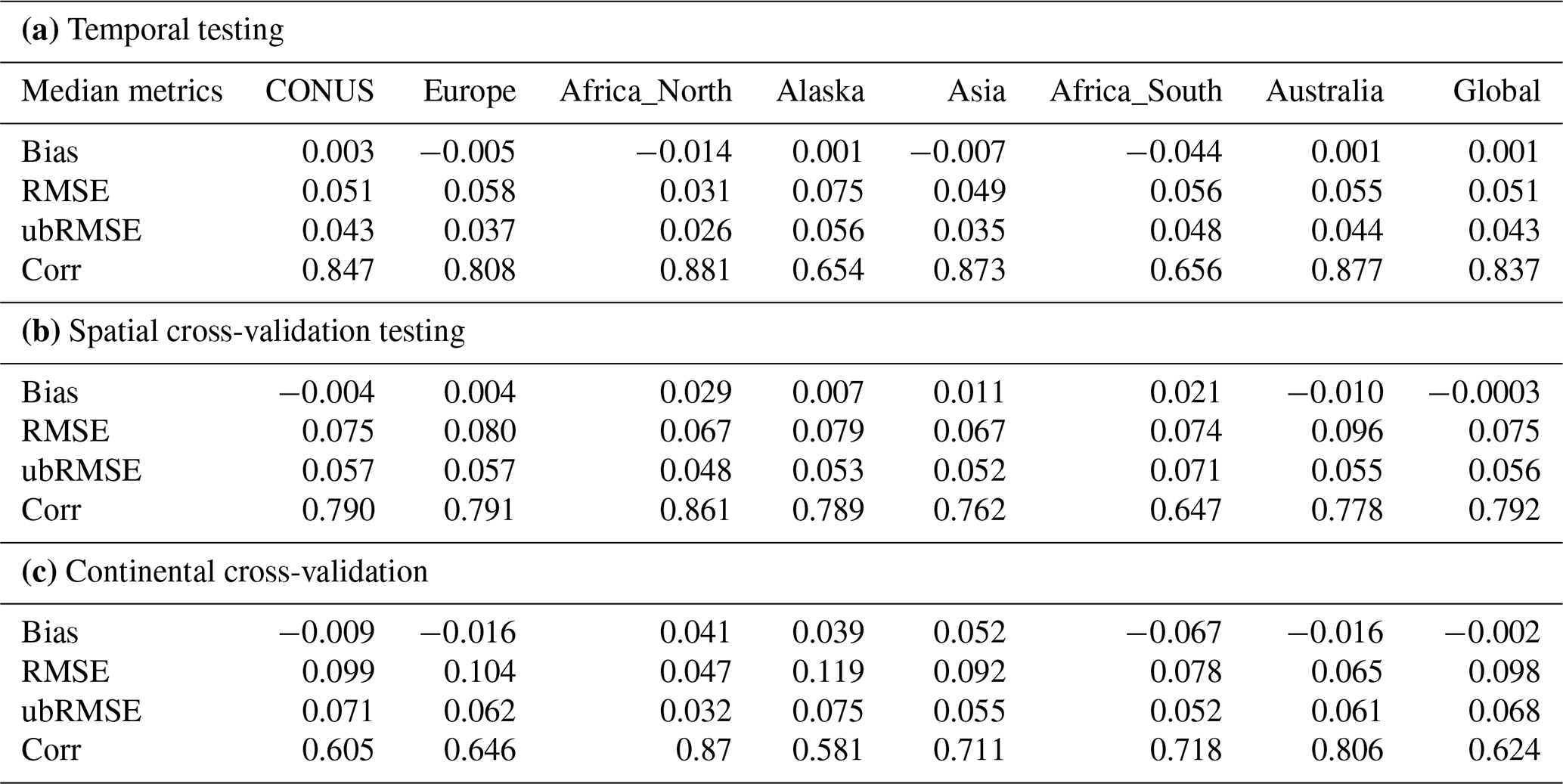
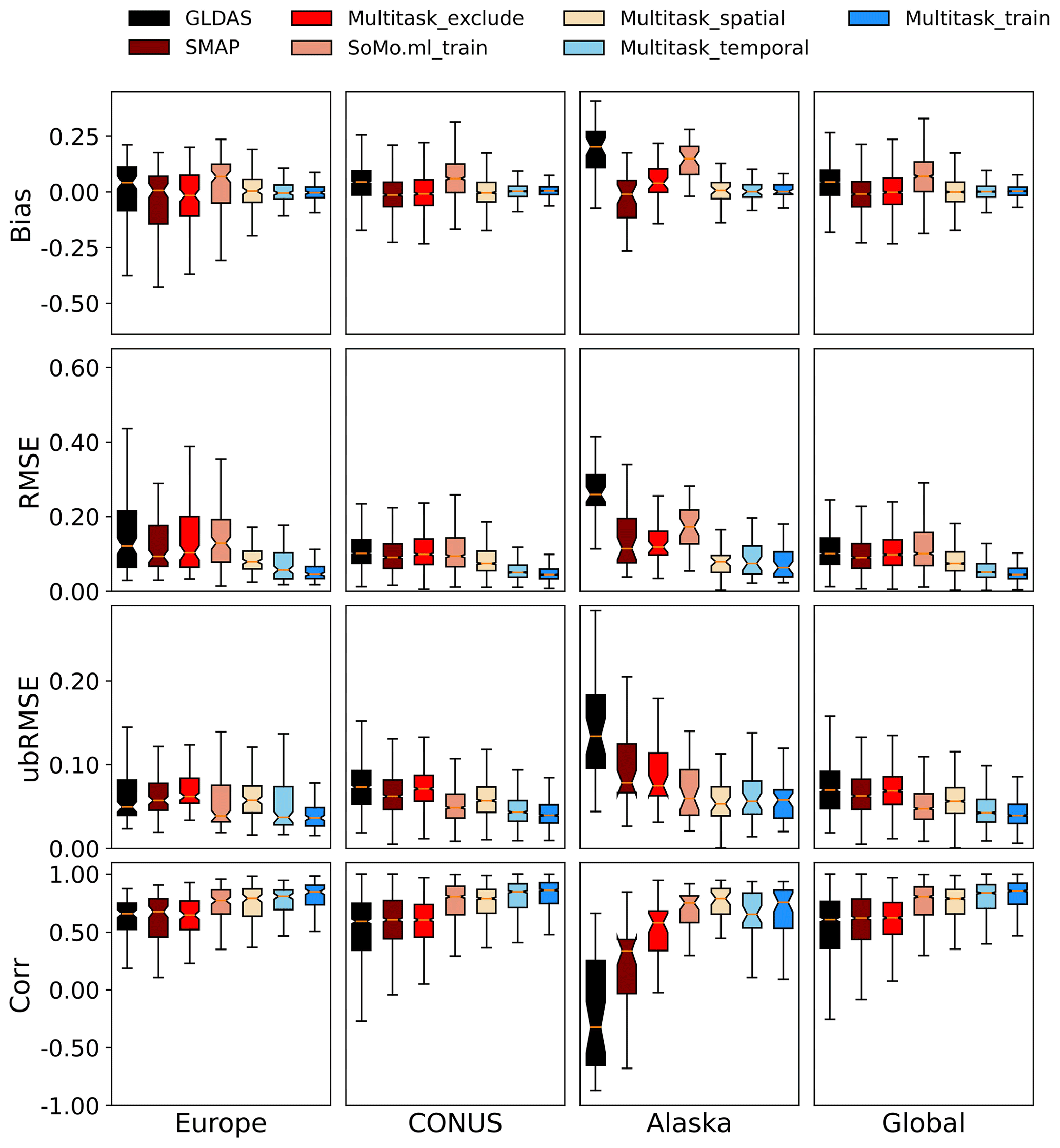
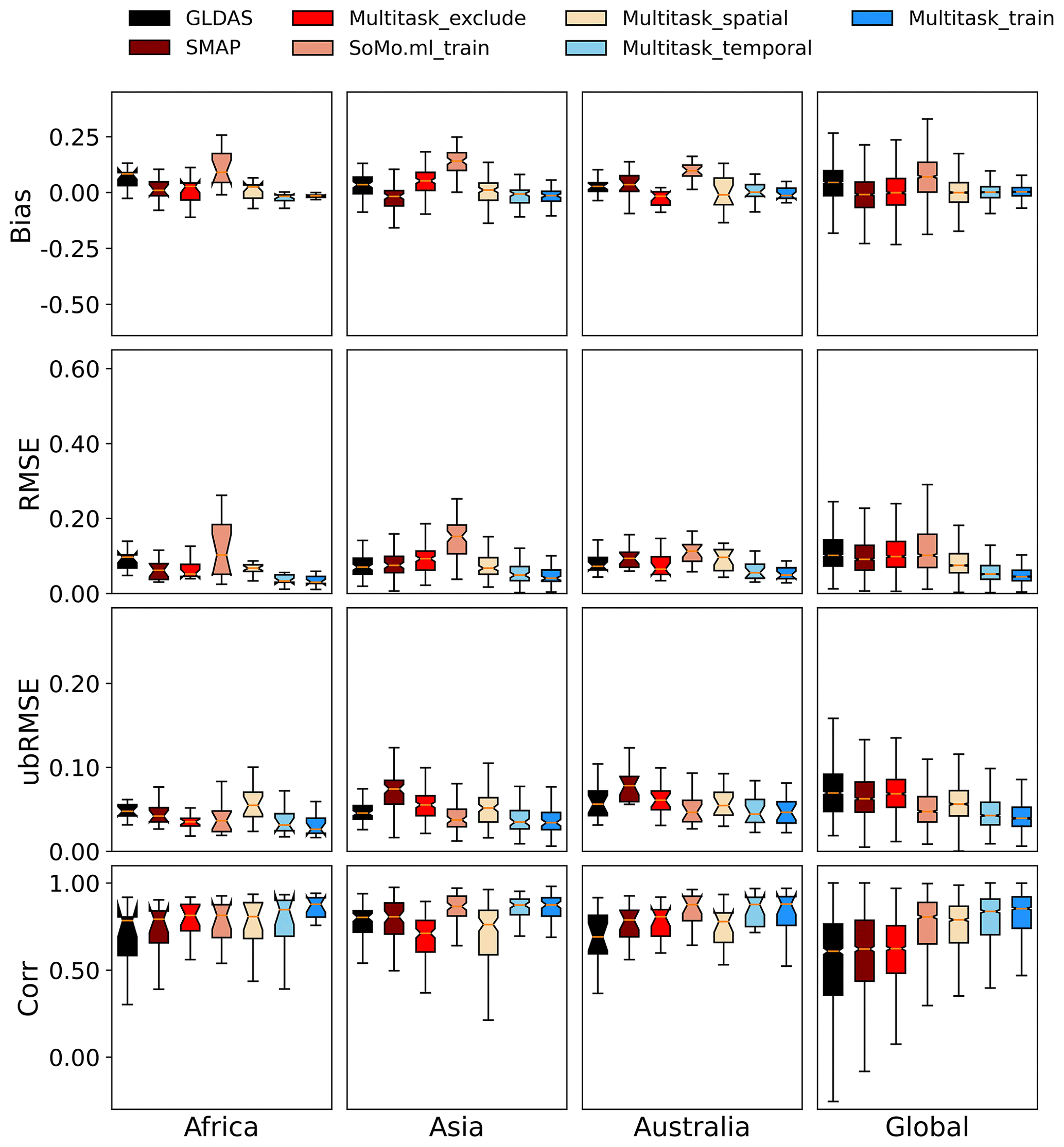
Figure 1Comparison of model performances for different continents in data-rich regions. Models from left to right are ranked from lowest to highest global correlation. We plotted results for the training period, as well as temporal, spatial, and cross-continental tests. “Multitask_exclude” means the cross-continent test: the models were tested on a continent, but sites from that continent were excluded from training. The SoMo.ml product shown here was trained on all sites in all time periods, and thus it is most comparable to our “Multitask_train” product.
The temporal tests (trained on some sites in one time period and tested on the same sites in another time period), which are used to establish a reference performance level, showed a strong ability for LSTM to capture soil moisture dynamics around the world, posting a global median correlation (R) of 0.837 (Table 1a and the sky-blue box, Multitask_temporal, in Figs. 1 and 2). Because LSTM has learned from the history of the sites, these test-region-aggregated temporal test metrics are normally higher than spatial tests (except for Alaska, which is to be discussed below) and reflect the inherent and geographically varying difficulties of soil moisture modeling in different regions. The temporal test R values for different regions are organized in the following order: Africa_North > Australia > Asia > CONUS > Europe > Africa_South ≅ Alaska. One immediately apparent observation is that this order is not related to the number of sites in each region or the density of sites. For example, the highest-ranking (in terms of R) regions are Africa_North, Australia, and Asia, which all are among the regions with the lowest counts of sites. Alaska has a relatively high site density but had the lowest median R, which could be attributed to the unique difficulties associated with frozen soil and thawing permafrost. This observation suggests that more training sites in these regions may not result in significantly better temporal test results at existing sites. Africa_South was more difficult than Africa_North, presumably because more sites are located in arid environments (LSTM has previously shown lower performance in such regions in the CONUS, as discussed in Feng et al., 2020). While these results show that there are some regions in the world that are more difficult to capture than others for the prediction of soil moisture, the overall results are encouraging. The model's performance over these regions indicates that the quality of the forcing (MSWEP+GPM+ERA5 precipitation) and soil characterization data is globally consistent.
Apart from Alaska, there were no particularly strong spatial patterns in either R or RMSE in the random spatial (cross-validation) tests (Fig. 3). Over the CONUS, there was a mild concentration of poorly performing sites in the northwest. In Europe, we found poorly performing sites in the central region, e.g., Hungary and Romania. Other than that, poorly performing sites were interspersed among the well-performing sites, suggesting that most of the causes of poor performance are local rather than climatic effects, which we will explore in Sect. 3.3. The cross-continental tests led to a widespread decrease in R, in comparison to the random spatial tests (Fig. 4). While some African sites, like those immediately south of the Sahara (Fig. 4c), had noticeably deteriorated performance, some other sites in fact improved, such as the three most southern sites in Africa_South (Fig. 4f).

Figure 3Metric distributions for the multitask model random spatial cross-validation tests. (I) Correlation and (II) RMSE of spatial cross-validation tests for (a) the CONUS, (b) Europe, (c) Africa_North, (d) Alaska, (e) Asia, (f) Africa_South, and (g) Australia. The training and testing periods were both from 1 April 2015 to 31 December 2020. Maps are made with Natural Earth imagery, no permission needed (Natural Earth, 2022).
3.2 Randomly sampled spatial cross-validation
The random spatial (randomly sampled cross-validation) tests, which examined the effect of spatial interpolation, showed record-breaking results despite their slight performance decline compared to the temporal tests. The global median R was 0.792, ubRMSE was 0.056, and RMSE was 0.075, all of which were slightly better than the CONUS median values (Table 1b and the wheat-colored box, Multitask_spatial, in Figs. 1 and 2). In contrast, the SMAP 9 km product and GLDAS had global median R values of 0.621 and 0.608, respectively. It should be noted that the numbers are not entirely comparable: SMAP 9 km and GLDAS were not calibrated fully on the sparse in situ sites. As expected, at the global scale, the training metrics were slightly better and had a smaller spread than those for the temporal and spatial tests. The LSTM-based SoMo.ml model obtained a median R of ∼0.6 for spatial cross-validation (Fig. 7 in O and Orth, 2021), while the downloadable SoMo.ml product (0.805, as shown in Figs. 1 and 2) was obtained based on training on all the sites and time periods and thus should in fact be compared to the our training period results (the rightmost box in each panel, Multitask_train; R=0.853). It should be noted that SoMo.ml has soil moisture for multiple depths, but we only explored the 5 cm product here. The closest model to the multitask LSTM is the one from Beck et al. (2021) (we do not have the data to plot their results), which was calibrated on 177 of the soil moisture sites and tested on the others. Their MSWEP+HBV (Hydrologiska Byråns Vattenbalansavdelning) model obtained a median R value of 0.78. Their performance is competitive and quite impressive for a process-based model, but unfortunately the HBV model only outputs a water storage value (in mm) that can be correlated to the fluctuation of observed soil moisture and not the soil moisture itself, and thus other metrics like bias cannot be calculated (additional linear transformations are required to obtain soil moisture, which introduces uncertainty). It would be interesting to explore how HBV or similar models would react to the cross-continental test below, where it may show some advantages.

Figure 4Metric distributions for the multitask model continental cross-validation tests. (I) Correlation and (II) RMSE of continental cross-validation tests for (a) the CONUS, (b) Europe, (c) Africa_North, (d) Alaska, (e) Asia, (f) Africa_South, and (g) Australia. The training and testing periods were both from 1 April 2015 to 31 December 2020. Maps are made with Natural Earth imagery, no permission needed (Natural Earth, 2022).
In general, the difference between the training and temporal tests is small, and thus we regard the model training error to be small. Switching from the temporal test to the random spatial test, most regions suffered a small decline in performance, suggesting that the impact of spatial heterogeneity is larger than the impact of temporal nonstationarity for soil moisture predictions. Regions seeing noticeable declines include the CONUS (from 0.847 to 0.790), Asia (0.873 to 0.762), and Australia (0.877 to 0.778), which could reflect the limited quality of soil texture data and processes that cannot be described by the input attributes. Alaska stood out as the exception (temporal test R=0.654; spatial test R=0.789), which is in fact consistent with our theory of errors discussed earlier and highlights the rapid changes facing Arctic regions. Alaska is challenging because it is the frontier of rapid changes in permafrost thawing and months of frozen ground conditions. As a result, temporal nonstationarity in that region trumps spatial heterogeneity. This observation suggests that the soil moisture dynamics in Arctic regions in the coming years will differ materially from those in the past decades.
Precipitation data quality exerts an important influence on the performance of the model but does not materially change the model comparisons. MSWEP is a high-quality global precipitation dataset (daily, 0.1∘ resolution) arising from blending multiple forcing datasets and correcting their biases (Beck et al., 2019). To support a fair comparison, we also ran our multitask model with the more widely used ERA5 precipitation data, which gave slightly lower-performing results. The multiscale model still outperformed reference products (Table S6). We further note that our previous CONUS results used the NLDAS-2 (North American Land Data Assimilation System Phase 2) forcing data, which are more customized toward North America, and obtained an R of 0.901 (Liu et al., 2022a). We thus conclude that the forcing dataset used has a moderate impact on results and needs to be the same for models to be fully comparable.
3.3 Cross-continental tests
As expected, model performances dropped significantly in the cross-continental test (testing on a continent where no training data was provided), but even under this adverse situation, the multitask LSTM model surpassed or equaled the performance of SMAP in all regions except Asia (Tables 1c, S4, Figs. 1 and 2). When the CONUS was included as a training region, the R value in all regions except Alaska stayed above 0.64. When both the CONUS and Europe were included (again, except for Alaska), there seemed to be a baseline performance level (R=0.70) that the model would not fall below, despite there being no training data from the test continent. For Africa and Australia, the advantages of the multitask model (multitask_exclude in Fig. 2) over SMAP or GLDAS are prominent. This suggests that we could consider the multitask LSTM model to be a viable product even in the no-data scenario.
Interestingly, the fewer sites a region had, the less impact there was by switching from the random spatial to the cross-continental test (Table 1c and the bright red boxes, Multitask_exclude, in Figs. 1 and 2). For Africa_North, Africa_South, and Australia, there was no decline from the random spatial test (Table 1b) to the cross-continental test (Table 1c). Asia saw a larger impact, with R dropping from 0.762 in the spatial test to 0.711 in the cross-continental test. We noticed precipitous drops for Alaska (median R from 0.789 to 0.581 – again suggesting soil moisture dynamics there are materially different from other parts of the world), Europe (0.791 to 0.646), and the CONUS (0.790 to 0.605). We thus conclude that when a region had very few sites but high heterogeneity, these sites only played a minor role in training the model, and thus removing them did not materially change the model. When a region had a large number of sites, like the CONUS or Europe, removing them substantially reduced the training data diversity. The quality of a DL model is a strong function of its training data – thus it would be severely weakened if a large part of its training data were removed.
It is also interesting that African, Australian, and Asian sites had good performance in this experiment. It seems to suggest their soil types and rainfall moisture responses have already been covered by similar sites in the CONUS and Europe, and thus the model was already sufficient. With diverse climates and landscapes ranging from desert to temperate forest and from croplands to wetlands, the CONUS networks play a dominant role in providing training on how soil moisture responds to different forcings, as modulated by the soil and landscape characteristics. We cannot know for certain that the model will work well in other parts of Africa and Asia until we have more in situ sites there. However, the current results at least can make us hopeful that the model will likely produce good results in some parts of the untrained world and will likely add value beyond satellite products.
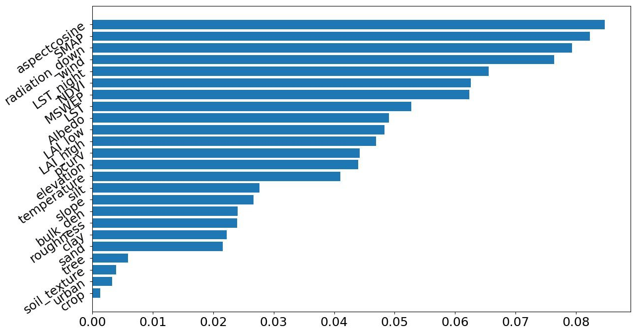
Figure 5The feature importance determined from a random forest (RF) model constructed to predict temporal test R using all the unduplicated category data presented in this paper as inputs. The correlation of this model is 0.6. Aspect, average soil moisture, and downward radiation are the top three factors. A separate gradient-boosted decision model was also trained and obtained a correlation of 0.77, and the top three important factors were similar: slope aspect, precipitation, and downward solar radiation.
3.4 Factorial influences on model performance
Due to LSTM's strong ability to fit to data, it can serve as a probe for process complexity (Liu et al., 2022a; Feng et al., 2022, 2020; Tsai et al., 2021): those sites that LSTM cannot adequately capture may contain complicated processes that are not well described by the inputs. The factorial importance analysis indicates that slope aspect, average soil moisture, and surface solar radiation downwards are the top three factors that influence the multitask LSTM model's R in the temporal test (Fig. 5). The RF model has a test correlation of 0.6 (with 80 % training data and 20 % test data), but its only purpose here is to provide a reading on the top three factors. We have also tried using gradient-boosted decision trees (Friedman, 2001), which produced a test correlation of 0.77, and the top three important factors were slope aspect, precipitation, and surface solar radiation downwards. Therefore, this model choice does not qualitatively affect our conclusions. As a reminder, the feature importance test is based on training random forest (RF) models with the inputs listed in Fig. 5, and R from the temporal test serves as the target. A high-ranking factor in Fig. 5 implies that it has influence not only on soil moisture but also on the predictability of soil moisture. It could be that in a certain range of this factor (the range may be conditional on other factors due to factorial interactions) there are not that many sites of this kind (it is a minority class that is not well represented in the training dataset) or that some latent processes become important. Nevertheless, due to the inherent limitations of machine learning, factorial importance is only a hypothesis rather than confirmed truth (Tsai et al., 2021). As a result, human interpretation of the results will be required. Because the sensitivity to radiation is somewhat difficult to interpret, here we focus on average soil moisture and aspect.
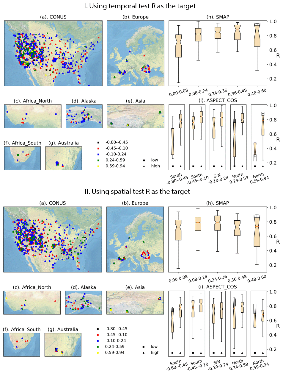
Figure 6Stratified analysis of the distribution of R values from (I) temporal and (II) spatial tests. (a–g) The maps show the global distribution of test sites as a function of average SMAP soil moisture value and aspect. The colors on the map represent aspect cosine. The average SMAP <0.08 sites are a minority class and are represented by squares. (h) The SMAP boxplot shows the distribution of R under different average soil moisture values (SMAP). (i) The aspect boxplot shows the distribution of R in different aspect cosine bins, where the left boxplot in each bin indicates SMAP ≦0.08, and the right boxplot in each bin indicates SMAP >0.08. The upper half of the figure, part I, shows temporal test R values (which characterize temporal nonstationarity), while the lower half of the figure, part II, shows spatial test R values, which characterize the effect of spatial heterogeneity. Maps are made with Natural Earth imagery, no permission needed (Natural Earth, 2022).
The model correlation in the temporal test generally rises as soil moisture goes up, until reaching the wettest regime (0.48–0.6), where its variability increases (Fig. 6Ih). The sites in the middle range tend to have continuity in soil moisture and regular rainfall patterns, which are most ideal for LSTM. There is a clear rising trend in R for the temporal test from dry to wet sites. The driest sites may be difficult to predict due to scarce but sudden rainfall events that quickly dry out, which reduces the usefulness of LSTM's memory capability. When we plotted the spatial test R (Fig. 6IIh), the pattern is similar but less pronounced, which suggests the driest sites are also more impacted by temporal non-stationarity than spatial heterogeneity because they have seen limited storm events. Toward the wettest regime, saturation often occurs, and soil moisture may be influenced by groundwater or flooding processes, which are difficult to account for.
Interestingly, aspect has a nonlinear effect that varies in different soil moisture regimes (Fig. 6Ii) due to its impact on shading and solar insolation. It is well known that aspect can have a predominant control on soil moisture and plants for dry sites, as witnessed by different vegetation densities and species and microbial communities on south-facing and north-facing slopes (Armesto and Martnez, 1978; Bennie et al., 2006; Xue et al., 2018). For the very dry sites (average SMAP <0.08), only those with mid-range aspects tended to have a decent correlation. The temporal test R (Fig. 6Ii) had a larger response to aspect than the spatial test R (Fig. 6IIi), which suggests this difficulty is not a result of too few training sites in space but a result of highly complex and nonstationary temporal trends in this combined range of average soil moisture and aspect. The north-facing dry slopes have a lower R, perhaps because of complex vegetation–soil moisture interactions in this regime, which may shift from year to year. The most south-facing dry slopes also have low R, perhaps because they approach the lower limit of soil moisture and can see large changes due to individual storm events. In contrast, for the wetter soil regimes, the role of aspect is reduced; we see noticeably reduced R only for the most south-facing slope (Fig. 6IIi). This reduced impact may be because soil moisture is no longer such a strong selector of vegetation species on these slopes, and thus the distinction of aspect becomes less important.
In the vast parts of Africa or Asia where soil moisture predictions are required but not well supported by in situ measurements, the analysis above can help us to anticipate challenges. At the hillslope scale, our predictions may have a larger error for those north-facing slopes in the dry regime and also straight south-facing slopes for the Northern Hemisphere (to be reversed for the Southern Hemisphere). The results highlight the importance of aspect controls on soil moisture and suggest that future models will need to represent its effect well before they can be accurate.
3.5 Further discussion
Our correlation is modestly higher than the previous state-of-the-art model, the well-calibrated conceptual hydrologic model, HBV. Even though that model does not simulate the physical quantity of soil moisture, it could be modified to have a module that does. However, to obtain suitable parameters on the global scale and improve the physical processes, we think adding differentiable programming to the model will give it the adaptive capability to learn from big data (Feng et al., 2022; Shen et al., 2023; Aboelyazeed et al., 2022; Bindas et al., 2022). It is possible that such a model may generalize better than LSTM over long distances due to the imposed physical constraints.
Typically, for many hydrologic applications (Fang et al., 2022; Feng et al., 2021; Liu et al., 2022a; Rahmani et al., 2021a), a spatial test is a tougher test than a temporal test for fully data-driven models, showing the strong impacts of spatial heterogeneity. This could either mean the inputs of the model do not completely describe the problem or that there are not enough sites in space with different combinations of input attributes for the model to fully resolve their impacts. Typically, spatial error can be gradually reduced if there are more training sites in space. However, in both Alaska (Fig. 1) and north-facing dry slopes around the world (Fig. 6IIi), temporal errors have exceeded spatial errors. Consistently, when we ran K-fold experiments with a higher K, it also did not result in noticeably different performances for the models (data not shown). These observations not only highlight the unique challenges of these places (rapid climate-driven changes and strong nonstationarity) but also suggest that the number of training sites is not a predominant issue for limiting the accuracy of soil moisture predictions.
While our product did not surpass SMAP by a large margin under the most stringent test (cross-continental), it is suitable as a long-term simulation tool, as it does not require near-real-time observations. Thus it can be used to assess future climate change impacts. It is also easy to further expand LSTM networks to enable “data integration” or “data assimilation”, which absorbs information from recent observations to improve future forecasts (Fang and Shen, 2020; Feng et al., 2020). Satellite observations could also be employed as the recent observations, as they could help to update LSTM's hidden states. Such assimilation typically results in a significant boost in performance and the elimination of bias. Compared to data assimilation with traditional models, we could skip the bias correction procedure, as LSTM models tend to have little bias and will adaptively learn to remove the bias by themselves. Data assimilation only has short-term impacts, however, and the value of the information content of the data will eventually wane as the simulation proceeds.
The LSTM-based SMAP modeling product is already deployed at scale via the operational agricultural advice application of PlantVillage, a nonprofit organization based at Penn State. We intend to put the multitask model into production alongside alternative estimates. This service is provided free of charge to farmers and extension services in Africa through the USAID Current and Emerging Threats to Crops Innovation Lab (CETC IL). PlantVillage currently scales out precipitation data to 13 million farmers per week in Kenya and Burkina Faso and believes the ability to complement this with more accurate information on soil moisture will be of large assistance to farmers coping with droughts and erratic weather as a result of climate change. It is also valuable to help farmers optimize fertilizer application rates, which has become even more critical due to the massive increase in fertilizer prices over the last 12 months.
When evaluated against sparse in situ soil moisture networks, the multitask LSTM model outperformed currently available satellite-based products, land surface models, and an alternative DL model across most continents. Judging by the 5-fold spatial test model results, the model had not only dramatically lower bias but also the highest correlation with in situ soil moisture networks. Learning from multiple data sources, the model can be deployed at large scales at a small computational cost and can be expanded to incorporate data assimilation capabilities. These features make it a suitable operational tool to democratize access to information for agriculture in developing regions. While we wish for more measurements in Africa for model training and validation, the results are at least encouraging. The model can utilize satellite-estimated soil moisture as one of the learning targets while also learning from in situ data, and thus it is well poised to provide higher-resolution outputs than the satellite-based products.
The LSTM model served as a probe for process complexity and showed that mean soil moisture and aspect have important controls on soil moisture predictability, while also showing that Arctic regions are inherently more difficult to predict due to rapid soil changes. For the dry slopes (average SMAP soil moisture <0.08) that face north, there could be complicated vegetation–soil moisture interactions that are difficult to predict. For the wetter slopes, the role of aspect becomes less prominent. Error analysis suggests that in these difficult regions, temporal errors can outweigh spatial errors, and thus having longer data records and monitoring most recent changes can be more important than adding more sites.
The multitask LSTM model can generalize well in highly data-sparse regions. Even in the worst-case scenario (no training data on a whole continent), the model was able to surpass SMAP's accuracy on most continents. It did seem to have some trouble generalizing to Alaska, where the soil dynamics are much different from other regions and are also experiencing rapid changes. However, it provided decent performance when tested in data-sparse continents where it has not been trained, like Africa and Australia, showing that these predictions can be beneficial for such regions where there are not a lot of published soil moisture datasets. This modeling success is partially due to the strong ability of the model to generalize but also because the soils in the known sites in Africa are similar to those in the training set. It is fortunate that the more intensively instrumented CONUS and Europe already contain a wide variety of soils and climates for training, without which the model would suffer greatly.
The multitask LSTM code and GSM3 soil moisture dataset can be downloaded at https://doi.org/10.5281/zenodo.7026036 (Liu et al., 2022b). Links to data sources have been provided in the Methods section.
The supplement related to this article is available online at: https://doi.org/10.5194/gmd-16-1553-2023-supplement.
CS conceived the study. JL ran the experiments and wrote an early draft. JL, DH, FR, KL, and CS edited the manuscript.
Chaopeng Shen and Kathryn Lawson have financial interests in HydroSapient, Inc., a company that could potentially benefit from the results of this research. This interest has been reviewed by the university in accordance with its individual conflict of interest policy for the purpose of maintaining the objectivity and integrity of research at The Pennsylvania State University.
Publisher’s note: Copernicus Publications remains neutral with regard to jurisdictional claims in published maps and institutional affiliations.
We thank the two reviewers and the editor for their constructive comments. We also thank the dataset providers for their effort in making data publicly accessible. Data access is a critical step toward enabling research on the global scale.
This work was supported by Google.org's AI Impacts Challenge Grant 1904-57775 and Gates Foundation award INV-018429. Chaopeng Shen was partially supported by National Science Foundation Award EAR-2221880 and OAC no. 1940190. Computation was partially supported by National Science Foundation Major Research Instrumentation Award PHY-2018280.
This paper was edited by Christoph Müller and reviewed by Richard Mills and one anonymous referee.
Aboelyazeed, D., Xu, C., Hoffman, F. M., Jones, A. W., Rackauckas, C., Lawson, K. E., and Shen, C.: A differentiable ecosystem modeling framework for large-scale inverse problems: demonstration with photosynthesis simulations, Biogeosciences Discuss. [preprint], https://doi.org/10.5194/bg-2022-211, in review, 2022.
Al Bitar, A., Mialon, A., Kerr, Y. H., Cabot, F., Richaume, P., Jacquette, E., Quesney, A., Mahmoodi, A., Tarot, S., Parrens, M., Al-Yaari, A., Pellarin, T., Rodriguez-Fernandez, N., and Wigneron, J.-P.: The global SMOS Level 3 daily soil moisture and brightness temperature maps, Earth Syst. Sci. Data, 9, 293–315, https://doi.org/10.5194/essd-9-293-2017, 2017.
Albergel, C., Dutra, E., Munier, S., Calvet, J.-C., Munoz-Sabater, J., de Rosnay, P., and Balsamo, G.: ERA-5 and ERA-Interim driven ISBA land surface model simulations: which one performs better?, Hydrol. Earth Syst. Sci., 22, 3515–3532, https://doi.org/10.5194/hess-22-3515-2018, 2018.
Al-Yaari, A., Wigneron, J.-P., Kerr, Y., Rodriguez-Fernandez, N., O'Neill, P. E., Jackson, T. J., De Lannoy, G. J. M., Al Bitar, A., Mialon, A., Richaume, P., Walker, J. P., Mahmoodi, A., and Yueh, S.: Evaluating soil moisture retrievals from ESA's SMOS and NASA's SMAP brightness temperature datasets, Remote Sens. Environ., 193, 257–273, https://doi.org/10.1016/j.rse.2017.03.010, 2017.
Amatulli, G., Domisch, S., Tuanmu, M.-N., Parmentier, B., Ranipeta, A., Malczyk, J., and Jetz, W.: A suite of global, cross-scale topographic variables for environmental and biodiversity modeling, Sci. Data, 5, 180040, https://doi.org/10.1038/sdata.2018.40, 2018.
Armesto, J. J. and Martnez, J. A.: Relations between vegetation structure and slope aspect in the Mediterranean region of Chile, J. Ecol., 66, 881–889, https://doi.org/10.2307/2259301, 1978.
Baraniuk, C.: Locust Swarms Are Getting So Big That We Need Radar to Track Them, Medium, https://onezero.medium.com/locust-swarms-are-getting-so-big-that-we-need-radar-to-track-them-dc79c06496a0 (last access: 1 August 2022), 2020.
Beaudoing, H. and Rodell, M.: GLDAS Noah Land Surface Model L4 3 hourly 0.25 x 0.25 degree V2.0 (GLDAS_NOAH025_3H 2.0), Greenbelt, Maryland, USA, Goddard Earth Sciences Data and Information Services Center (GES DISC) [data set], https://doi.org/10.5067/342OHQM9AK6Q, 2019.
Beck, H. E., Wood, E. F., Pan, M., Fisher, C. K., Miralles, D. G., Dijk, A. I. J. M. van, McVicar, T. R., and Adler, R. F.: MSWEP V2 Global 3-Hourly 0.1∘ Precipitation: Methodology and Quantitative Assessment, B. Am. Meteorol. Soc., 100, 473–500, https://doi.org/10.1175/BAMS-D-17-0138.1, 2019.
Beck, H. E., Pan, M., Miralles, D. G., Reichle, R. H., Dorigo, W. A., Hahn, S., Sheffield, J., Karthikeyan, L., Balsamo, G., Parinussa, R. M., van Dijk, A. I. J. M., Du, J., Kimball, J. S., Vergopolan, N., and Wood, E. F.: Evaluation of 18 satellite- and model-based soil moisture products using in situ measurements from 826 sensors, Hydrol. Earth Syst. Sci., 25, 17–40, https://doi.org/10.5194/hess-25-17-2021, 2021.
Bennie, J., Hill, M. O., Baxter, R., and Huntley, B.: Influence of slope and aspect on long-term vegetation change in British chalk grasslands, J. Ecol., 94, 355–368, https://doi.org/10.1111/j.1365-2745.2006.01104.x, 2006.
Bentley, A. R., Donovan, J., Sonder, K., Baudron, F., Lewis, J. M., Voss, R., Rutsaert, P., Poole, N., Kamoun, S., Saunders, D. G. O., Hodson, D., Hughes, D. P., Negra, C., Ibba, M. I., Snapp, S., Sida, T. S., Jaleta, M., Tesfaye, K., Becker-Reshef, I., and Govaerts, B.: Near- to long-term measures to stabilize global wheat supplies and food security, Nat. Food, 3, 483–486, https://doi.org/10.1038/s43016-022-00559-y, 2022.
Bindas, T., Tsai, W.-P., Liu, J., Rahmani, F., Feng, D., Bian, Y., Lawson, K., and Shen, C.: Improving large-basin streamflow simulation using a modular, differentiable, learnable graph model for routing, ESS Open Archive [preprint], https://doi.org/10.1002/essoar.10512512.1, 2022.
de Jeu, R. and Owe, M.: AMSR2/GCOM-W1 surface soil moisture (LPRM) L3 1 day 10 km x 10 km ascending V001, Goddard Earth Sciences Data and Information Services Center (GES DISC) (Bill Teng), Greenbelt, MD, USA, Goddard Earth Sciences Data and Information Services Center (GES DISC) [data set], https://doi.org/10.5067/B0GHODHJLDA8, 2013.
Didan, K.: MOD13C2: MODIS/Terra Vegetation Indices Monthly L3 Global 0.05Deg CMG version 6, NASA EOSDIS Land Processes DAAC [data set], https://doi.org/10.5067/MODIS/MOD13C2.006, 2015.
Dorigo, W. A., Wagner, W., Hohensinn, R., Hahn, S., Paulik, C., Xaver, A., Gruber, A., Drusch, M., Mecklenburg, S., van Oevelen, P., Robock, A., and Jackson, T.: The International Soil Moisture Network: a data hosting facility for global in situ soil moisture measurements, Hydrol. Earth Syst. Sci., 15, 1675–1698, https://doi.org/10.5194/hess-15-1675-2011, 2011.
Dorigo, W. A., Xaver, A., Vreugdenhil, M., Gruber, A., Hegyiová, A., Sanchis-Dufau, A. D., Zamojski, D., Cordes, C., Wagner, W., and Drusch, M.: Global automated quality control of in situ soil moisture data from the international soil moisture network, Vadose Zone J., 12, vzj2012.0097, https://doi.org/10.2136/vzj2012.0097, 2013.
Ellenburg, W. L., Mishra, V., Roberts, J. B., Limaye, A. S., Case, J. L., Blankenship, C. B., and Cressman, K.: Detecting desert locust breeding grounds: A satellite-assisted modeling approach, Remote Sens., 13, 1276, https://doi.org/10.3390/rs13071276, 2021.
Entekhabi, D.: The Soil Moisture Active Passive (SMAP) mission, P. IEEE, 98, 704–716, https://doi.org/10/bz3xhb, 2010.
ESA: Land Cover CCI Product User Guide Version 2, http://maps.elie.ucl.ac.be/CCI/viewer/download/ESACCI-LC-Ph2-PUGv2_2.0.pdf (last access: 1 August 2022), 2017.
Fang, K. and Shen, C.: Near-real-time forecast of satellite-based soil moisture using long short-term memory with an adaptive data integration kernel, J. Hydrometeorol., 21, 399–413, https://doi.org/10.1175/jhm-d-19-0169.1, 2020.
Fang, K., Shen, C., Kifer, D., and Yang, X.: Prolongation of SMAP to spatiotemporally seamless coverage of continental U.S. using a deep learning neural network, Geophys. Res. Lett., 44, 11030–11039, https://doi.org/10.1002/2017gl075619, 2017.
Fang, K., Pan, M., and Shen, C.: The value of SMAP for long-term soil moisture estimation with the help of deep learning, IEEE T. Geosci. Remote, 57, 2221–2233, https://doi.org/10/gghp3v, 2019.
Fang, K., Kifer, D., Lawson, K., Feng, D., and Shen, C.: The data synergy effects of time-series deep learning models in hydrology, Water Resour. Res., 58, e2021WR029583, https://doi.org/10.1029/2021WR029583, 2022.
FAO, IIASA, ISRIC, ISSCAS, and JRC: Harmonized World Soil Database (version 1.2), FAO IIASA, ISRIC, ISSCAS, and JRC [data set], http://www.fao.org/soils-portal/data-hub/soil-maps-and-databases/harmonized-world-soil-database-v12/en/ (last access: 1 August 2022), 2012.
Feng, D., Fang, K., and Shen, C.: Enhancing streamflow forecast and extracting insights using long-short term memory networks with data integration at continental scales, Water Resour. Res., 56, e2019WR026793, https://doi.org/10.1029/2019WR026793, 2020.
Feng, D., Lawson, K., and Shen, C.: Mitigating prediction error of deep learning streamflow models in large data-sparse regions with ensemble modeling and soft data, Geophys. Res. Lett., 48, e2021GL092999, https://doi.org/10.1029/2021GL092999, 2021.
Feng, D., Liu, J., Lawson, K., and Shen, C.: Differentiable, learnable, regionalized process-based models with multiphysical outputs can approach state-of-the-art hydrologic prediction accuracy, Water Resour. Res., 58, e2022WR032404, https://doi.org/10.1029/2022WR032404, 2022.
Fischer, G., Nachtergaele, F., Prieler, S., van Velthuizen, H. T., Verelst, L., and Wiberg, D.: Global Agro-Ecological Zones Assessment for Agriculture (GAEZ 2008), IIASA Laxenburg, Austria and FAO, Rome, Italy, 2008.
Friedman, J. H.: Greedy Function Approximation: A Gradient Boosting Machine, Ann. Stat., 29, 1189–1232, 2001.
Gauch, M., Mai, J., and Lin, J.: The Proper Care and Feeding of CAMELS: How Limited Training Data Affects Streamflow Prediction, Environ. Modell. Softw., 135, 104926, https://doi.org/10.1016/j.envsoft.2020.104926, 2021.
Hochreiter, S. and Schmidhuber, J.: Long Short-Term Memory, Neural. Comput., 9, 1735–1780, https://doi.org/10.1162/neco.1997.9.8.1735, 1997.
Hrachowitz, M., Savenije, H. H. G., Blöschl, G., McDonnell, J. J., Sivapalan, M., Pomeroy, J. W., Arheimer, B., Blume, T., Clark, M. P., Ehret, U., Fenicia, F., Freer, J. E., Gelfan, A., Gupta, H. V., Hughes, D. A., Hut, R. W., Montanari, A., Pande, S., Tetzlaff, D., Troch, P. A., Uhlenbrook, S., Wagener, T., Winsemius, H. C., Woods, R. A., Zehe, E., and Cudennec, C.: A decade of Predictions in Ungauged Basins (PUB)–a review, Hydrol. Sci. J., 58, 1198–1255, https://doi.org/10/gfsq5q, 2013.
Huffman, G. J., Stocker, E. F., Bolvin, D. T., Nelkin, E. J., and Tan, J.: GPM IMERG Final Precipitation L3 1 day 0.1 degree x 0.1 degree V06 (GPM_3IMERGDF 06), edited by: Andrey Savtchenko, Greenbelt, MD, Goddard Earth Sciences Data and Information Services Center (GES DISC) [data set], https://doi.org/10.5067/GPM/IMERGDF/DAY/06, 2019.
Hunter-Jones, P.: Egg development in the Desert Locust (Schistocerca gregaria Forsk.) in relation to the availability of water, Proc. R. Entomol. Soc. A, 39, 25–33, https://doi.org/10.1111/j.1365-3032.1964.tb00781.x, 1964.
Kerr, Y. H., Waldteufel, P., Wigneron, J.-P., Delwart, S., Cabot, F., Boutin, J., Escorihuela, M.-J., Font, J., Reul, N., Gruhier, C., Juglea, S. E., Drinkwater, M. R., Hahne, A., Martín-Neira, M., and Mecklenburg, S.: The SMOS mission: New tool for monitoring key elements of the global water cycle, P. IEEE, 98, 666–687, https://doi.org/10/b9szx6, 2010.
Kratzert, F., Klotz, D., Shalev, G., Klambauer, G., Hochreiter, S., and Nearing, G.: Towards learning universal, regional, and local hydrological behaviors via machine learning applied to large-sample datasets, Hydrol. Earth Syst. Sci., 23, 5089–5110, https://doi.org/10.5194/hess-23-5089-2019, 2019.
Liu, J., Rahmani, F., Lawson, K., and Shen, C.: A multiscale deep learning model for soil moisture integrating satellite and in situ data, Geophys. Res. Lett., 49, e2021GL096847, https://doi.org/10.1029/2021GL096847, 2022a.
Liu, J., Hughes, D., Rahmani, F., Lawson, K., and Shen, C.: Global Soil Moisture Dataset From a Multitask Model (GSM3), Zenodo [data set], https://doi.org/10.5281/zenodo.7344484, 2022b.
Meyal, A. Y., Versteeg, R., Alper, E., Johnson, D., Rodzianko, A., Franklin, M., and Wainwright, H.: Automated cloud based long short-term memory neural network based SWE prediction, Front. Water, 2, 1–12, https://doi.org/10.3389/frwa.2020.574917, 2020.
Muñoz Sabater, J.: ERA5-Land hourly data from 1950 to present, Copernicus Climate Change Service (C3S) Climate Data Store (CDS) [data set], https://doi.org/10.24381/cds.e2161bac, 2019.
Narasimhan, B. and Srinivasan, R.: Development and evaluation of Soil Moisture Deficit Index (SMDI) and Evapotranspiration Deficit Index (ETDI) for agricultural drought monitoring, Agr. Forest Meteorol., 133, 69–88, https://doi.org/10/fq9wdv, 2005.
Natural Earth: Free vector and raster map data, Natural Earth [data set], https://www.naturalearthdata.com/, last access: 1 August 2022.
Norbiato, D., Borga, M., Degli Esposti, S., Gaume, E., and Anquetin, S.: Flash flood warning based on rainfall thresholds and soil moisture conditions: An assessment for gauged and ungauged basins, J. Hydrol., 362, 274–290, https://doi.org/10/dtw4hm, 2008.
Nuwer, R.: As Locusts Swarmed East Africa, This Tech Helped Squash Them, N. Y. Times, 8th April, https://www.nytimes.com/2021/04/08/science/locust-swarms-africa.html (last access: 1 August 2022), 2021.
O, S. and Orth, R.: Global soil moisture data derived through machine learning trained with in-situ measurements, Sci. Data, 8, 170, https://doi.org/10.1038/s41597-021-00964-1, 2021.
O'Neill, P. E., Chan, S., Njoku, E. G., Jackson, T., Bindlish, R., Chaubell, J., and Colliander, A.: SMAP Enhanced L3 Radiometer Global and Polar Grid Daily 9 km EASE-Grid Soil Moisture, Version 5 (SPL3SMP_E), Boulder, Colorado USA, NASA National Snow and Ice Data Center Distributed Active Archive Center [data set], https://doi.org/10.5067/4DQ54OUIJ9DL, 2021.
Owe, M., de Jeu, R., and Holmes, T.: Multisensor historical climatology of satellite-derived global land surface moisture, J. Geophys. Res., 113, 1–17, https://doi.org/10.1029/2007JF000769, 2008.
Pedregosa, F., Varoquaux, G., Gramfort, A., Michel, V., Thirion, B., Grisel, O., Blondel, M., Prettenhofer, P., Weiss, R., and Dubourg, V.: Scikit-learn: Machine learning in Python, J. Mach. Learn. Res., 12, 2825–2830, 2011.
Rahmani, F., Shen, C., Oliver, S., Lawson, K., and Appling, A.: Deep learning approaches for improving prediction of daily stream temperature in data-scarce, unmonitored, and dammed basins, Hydrol. Process., 35, e14400, https://doi.org/10.1002/hyp.14400, 2021a.
Rahmani, F., Lawson, K., Ouyang, W., Appling, A., Oliver, S., and Shen, C.: Exploring the exceptional performance of a deep learning stream temperature model and the value of streamflow data, Environ. Res. Lett., 16, 024025, https://doi.org/10.1088/1748-9326/abd501, 2021b.
Rodell, M., Houser, P. R., Jambor, U., Gottschalck, J., Mitchell, K., Meng, C.-J., Arsenault, K., Cosgrove, B., Radakovich, J., Bosilovich, M., Entin, J. K., Walker, J. P., Lohmann, D., and Toll, D.: The Global Land Data Assimilation System, B. Am. Meteorol. Soc., 85, 381–394, https://doi.org/10.1175/BAMS-85-3-381, 2004.
Schaaf, C. and Wang, Z.: MODIS/Terra+Aqua BRDF/Albedo Daily L3 Global – 500m V061, NASA EOSDIS Land Processes DAAC [data set], https://doi.org/10.5067/MODIS/MCD43A3.061, 2021.
Sheffield, J. and Wood, E. F.: Global trends and variability in soil moisture and drought characteristics, 1950–2000, from observation-driven simulations of the terrestrial hydrologic cycle, J. Climate, 21, 432–458, https://doi.org/10.1175/2007JCLI1822.1, 2008.
Shen, C.: A transdisciplinary review of deep learning research and its relevance for water resources scientists, Water Resour. Res., 54, 8558–8593, https://doi.org/10.1029/2018wr022643, 2018.
Shen, C., Appling, A. P., Gentine, P., Bandai, T., Gupta, H., Tartakovsky, A., Baity-Jesi, M., Fenicia, F., Kifer, D., Li, L., Liu, X., Ren, W., Zheng, Y., Harman, C. J., Clark, M., Farthing, M., Feng, D., Kumar, P., Aboelyazeed, D., Rahmani, F., Beck, H. E., Bindas, T., Dwivedi, D., Fang, K., Höge, M., Rackauckas, C., Roy, T., Xu, C., and Lawson, K.: Differentiable modeling to unify machine learning and physical models and advance Geosciences, arXiv [preprint], https://doi.org/10.48550/arXiv.2301.04027, 10 January 2023.
Support CATDS: CATDS-PDC L3SM Simple UDP – 1 day soil moisture Simple User Data Product from SMOS satellite, CATDS (CNES, IFREMER, CESBIO) [data set] https://doi.org/10.12770/8db7102b-1b22-4db3-949d-e51269417aae, 2022.
Tsai, W.-P., Feng, D., Pan, M., Beck, H., Lawson, K., Yang, Y., Liu, J., and Shen, C.: From calibration to parameter learning: Harnessing the scaling effects of big data in geoscientific modeling, Nat. Commun., 12, 5988, https://doi.org/10.1038/s41467-021-26107-z, 2021.
UN WFP: Stop locusts in East Africa now or pay much more to help people later, U. N. UN World Food Programme WFP, 14th February, https://www.wfp.org/news/stop-locusts-east-africa-now-or-pay-much-more-help-people-later-wfp (last access: 1 August 2022), 2020.
Wan, Z., Hook, S., and Hulley, G.: MODIS/Aqua Land Surface Temperature/Emissivity Daily L3 Global 1km SIN Grid V061, NASA EOSDIS Land Processes DAAC [data set], https://doi.org/10.5067/MODIS/MYD11A1.061, 2021.
Xue, R., Yang, Q., Miao, F., Wang, X., Shen, Y., Xue, R., Yang, Q., Miao, F., Wang, X., and Shen, Y.: Slope aspect influences plant biomass, soil properties and microbial composition in alpine meadow on the Qinghai-Tibetan plateau, J. Soil Sci. Plant Nut., 18, 1–12, https://doi.org/10.4067/S0718-95162018005000101, 2018.
Yang, Z.-L., Niu, G.-Y., Mitchell, K. E., Chen, F., Ek, M. B., Barlage, M., Longuevergne, L., Manning, K., Niyogi, D., Tewari, M., and Xia, Y.: The community Noah land surface model with multiparameterization options (Noah-MP): 2. Evaluation over global river basins, J. Geophys. Res.-Atmos., 116, D12110, https://doi.org/10.1029/2010JD015140, 2011.
Zhi, W., Feng, D., Tsai, W.-P., Sterle, G., Harpold, A., Shen, C., and Li, L.: From hydrometeorology to river water quality: Can a deep learning model predict dissolved oxygen at the continental scale?, Environ. Sci. Technol., 55, 2357–2368, https://doi.org/10.1021/acs.est.0c06783, 2021.