A mixed finite-element discretisation of the shallow-water equations

This paper introduces a mixed finite-element shallow-water model on the sphere. The mixed finite-element approach is used as it has been shown to be both accurate and highly scalable for parallel architecture. Key features of the model are an iterated semi-implicit time-stepping scheme, a finite-volume transport scheme, and the cubed sphere grid. The model is tested on a number of standard spherical shallow-water test cases. Results show that the model produces similar results to other shallow-water models in the literature.

1 Introduction

The dynamical core of an atmospheric model numerically approximates the solution to the governing fluid dynamics equations that determine the evolution of the atmosphere. An operational dynamical core must be both accurate, to give confidence in the forecast, and efficient, to produce a forecast in the desired time frame. Current supercomputer architectures focus on using an increasing number of processors to decrease runtime, and so future dynamical cores must be suitable for massively parallel architecture. Key aspects of the dynamical core that will greatly affect both accuracy and parallel scalability are the type of grid and the numerical methods used to discretise the equations.

Traditionally, atmospheric models used a latitude–longitude grid (Wood et al., 2014). However, the convergence of the meridians at the pole leads to a computational bottleneck, and thus the latitude–longitude grid is not suitable for future supercomputers. Hence, a number of different approaches to gridding the sphere without a pole have been developed and used in dynamical cores, such as icosahedral grids and the yin–yang grid (Staniforth and Thuburn, 2012). One such promising grid is the cubed sphere, which uses quadrilateral cells on six panels that cover the sphere (Ronchi et al., 1996).

The choice of numerical methods used in a dynamical core will affect both the accuracy and the efficiency of the model. High-order methods generally improve accuracy but increase the computational cost. There are a variety of spatial methods (for example, finite-difference, finite-volume, semi-Lagrangian) and temporal methods (for example, explicit, semi-implicit, horizontally explicit, vertically implicit) used in atmospheric models by different operational centres and modelling groups (see Ullrich et al., 2017, and references within). The mixed finite-element method of Cotter and Shipton (2012) and Cotter and Thuburn (2014) is a spatial method that allows high-order schemes to be defined whilst retaining good parallel properties (Melvin et al., 2019). Mixed finite elements retain many properties of C-grid finite-difference and finite-volume methods, such as good numerical dispersion relations. They also have the advantage of not requiring orthogonal grids (Cotter and Shipton, 2012), better consistency of the Coriolis operator (Thuburn and Cotter, 2015), and the flexibility to increase accuracy by using higher-order elements. In practice, most current atmospheric dynamical cores aim for second-order accuracy overall (with the transport scheme often higher order) (Wood et al., 2014). For this reason the lowest-order mixed finite-element method will be a building block of the model described in this article.

The shallow-water equations are an important step in testing the methods used for the development of a dynamical core (Williamson et al., 1992). The shallow-water equations contain many of the properties of the full atmospheric governing equations but with a reduction in complexity. In practice, if a method is not good enough (by whatever metric) for a shallow-water model, it will not be good enough for an atmospheric dynamical core. This allows the methods to be evaluated in a simpler setting and design decisions to be made early in development.

This document presents a novel mixed finite-element discretisation, extending that of Melvin et al. (2019) for atmospheric dynamics in Cartesian geometry, of the rotating shallow-water equations in a spherical domain. This is the natural next step from Melvin et al. (2019) in the development of a three-dimensional dynamical core in spherical geometry, allowing the impact of the chosen spherical grid to be investigated in a simplified context using an evolution of the same numerics. As with the model of Melvin et al. (2019), the shallow-water discretisation presented here has been developed in the LFRic framework: see Adams et al. (2019). Key components of the model are the semi-implicit iterated time-stepping scheme and the finite-volume transport. The governing shallow-water equations are given in Sect. 2. The discretisation, including the spatial and temporal aspects, is given in Sect. 3, the finite-volume transport scheme is described in Sect. 4, and the solution procedure is outlined in Sect. 5. Results from standard shallow-water test suites are given in Sect. 7, with a concluding summary in Sect. 8.

2 Governing equations

The shallow-water equations in a rotating domain are given in vector-invariant form by

$$\begin{array}{}\text{(1)}& {\displaystyle \frac{\partial \mathit{u}}{\partial t}}+q\mathrm{\Phi }{\mathit{u}}^{⟂}+\mathrm{\nabla }\left(K+\mathrm{\Phi }+{\mathrm{\Phi }}_{\mathrm{s}}\right)=\mathrm{0},\text{(2)}& {\displaystyle \frac{\partial \mathrm{\Phi }}{\partial t}}+\mathrm{\nabla }\cdot \left(\mathit{u}\mathrm{\Phi }\right)=\mathrm{0},\end{array}$$

where $\mathit{u}=(u,v)$ is the velocity, Φ=gh is the geopotential (with gravity g and free surface height h), Φ_s is the surface geopotential, and $K\equiv \mathrm{1}/\mathrm{2}|\mathit{u}{|}^{\mathrm{2}}$ is the kinetic energy. The perpendicular operator is defined by $(u,v{)}^{⟂}=(-v,u)$.

The potential vorticity (PV) q is defined as

$$\begin{array}{}\text{(3)}& q={\displaystyle \frac{{\mathrm{\nabla }}^{⟂}\cdot \mathit{u}+f}{\mathrm{\Phi }}},\end{array}$$

where f is the Coriolis parameter and ${\mathrm{\nabla }}^{⟂}\cdot \equiv \mathit{k}\cdot \mathrm{\nabla }\times$, and taking the curl of Eq. (1) gives a conservative transport equation for PV:

$$\begin{array}{}\text{(4)}& {\displaystyle \frac{\partial \mathrm{\Phi }q}{\partial t}}+\mathrm{\nabla }\cdot \left(\mathit{u}\mathrm{\Phi }q\right)=\mathrm{0}.\end{array}$$

3 Discretisation

The governing Eqs. (1) and (2) are discretised in time using a two-time-level iterated implicit scheme (Sect. 3.1) and in space using a mixed finite-element method (Sect. 3.2) for the wave-dynamic terms and a high-order upwind finite-volume scheme (Sect. 4) for the advection terms. This process is an extension to the shallow-water equations on the sphere of Melvin et al. (2019), who presented a similar discretisation in a three-dimensional Cartesian domain.

3.1 Temporal discretisation

To achieve second-order temporal accuracy, a time-centred approach is used. The target discretisation, as in Melvin et al. (2019), is a two-time-level iterated implicit scheme where terms responsible for the fast-wave dynamics are treated by the iterative semi-implicit scheme and the transport terms (those involving the mass flux in Eq. 2 and the potential vorticity in Eq. 1) are computed using a high-order, upwind, explicit finite-volume scheme. Taking Eqs. (1) and (2) and applying this discretisation results in

$$\begin{array}{}\text{(5)}& {\displaystyle }{\mathit{\delta }}_t\mathit{u}+{\mathcal{F}}^{⟂}\left(q^n{\mathrm{\Phi }}^n,{\stackrel{\mathrm{‾}}{\mathit{u}}}^{\mathrm{1}/\mathrm{2}}\right)+\mathrm{\nabla }{\stackrel{\mathrm{‾}}{\left(K+\mathrm{\Phi }+{\mathrm{\Phi }}_{\mathrm{s}}\right)}}^{\mathit{\alpha }}& {\displaystyle }=\mathrm{0},\text{(6)}& {\displaystyle }{\mathit{\delta }}_t\mathrm{\Phi }+\mathrm{\nabla }\cdot \mathcal{F}\left({\mathrm{\Phi }}^n,{\stackrel{\mathrm{‾}}{\mathit{u}}}^{\mathrm{1}/\mathrm{2}}\right)& {\displaystyle }=\mathrm{0},\end{array}$$

where ${\mathit{\delta }}_{t}s\equiv \left(s^{n+\mathrm{1}}-s^n\right)/\mathrm{\Delta }t$, ${\stackrel{\mathrm{‾}}{s}}^{\mathit{\alpha }}\equiv \mathit{\alpha }{s}^{n+\mathrm{1}}+\left(\mathrm{1}-\mathit{\alpha }\right)s^n$, and 𝓕(s,u) are the fluxes computed by the transport scheme of variable s by wind field u. We use $\mathit{\alpha }=\mathrm{1}/\mathrm{2}$ to achieve the second order centred in the time scheme.

3.2 Mixed finite-element discretisation

The mixed finite-element formulation in two spatial dimensions requires the specification of three finite-element function spaces: ${\mathbb{V}}_{\mathrm{0}},{\mathbb{V}}_{\mathrm{1}},{\mathbb{V}}_{\mathrm{2}}$ (cf. the four function spaces ${\mathbb{W}}_i,i=\mathrm{0}\mathrm{\dots }\mathrm{3}$ used in Melvin et al., 2019). The scalar spaces are an H₁ space consisting of point-wise scalars, 𝕍₀ (zero forms), or an L₂ space consisting of area-integrated scalars, 𝕍₂ (two forms). There are two choices for the vector space 𝕍₁ corresponding to either ${\mathbb{V}}_{\mathrm{1}}^C$, a H_curl space of circulation vectors, or ${\mathbb{V}}_{\mathrm{1}}^D$, a H_div space of flux vectors. Each choice has an associated discrete de Rham complex,

$$\begin{array}{}\text{(7)}& {\mathbb{V}}_{\mathrm{0}}\stackrel{\mathrm{\nabla }}{⟶}{\mathbb{V}}_{\mathrm{1}}^C\stackrel{\mathit{k}\cdot \mathrm{\nabla }\times }{⟶}{\mathbb{V}}_{\mathrm{2}}\end{array}$$

for curl-conforming vectors and

$$\begin{array}{}\text{(8)}& {\mathbb{V}}_{\mathrm{0}}\stackrel{\mathit{k}\times \mathrm{\nabla }}{⟶}{\mathbb{V}}_{\mathrm{1}}^D\stackrel{\mathrm{\nabla }\cdot }{⟶}{\mathbb{V}}_{\mathrm{2}}\end{array}$$

for div-conforming vectors. For this paper only the div-conforming complex Eq. (8) will be considered: ${\mathbb{V}}_{\mathrm{1}}\equiv {\mathbb{V}}_{\mathrm{1}}^D$, with u∈𝕍₁ and Φ∈𝕍₂. This is analogous to the standard C-grid staggering (Arakawa and Lamb, 1977) where the normal components of the velocity vector are stored at the cell edges. The div-conforming complex, with the locations of the prognostic variables u, v, and Φ, is shown in Fig. 1.

Figure 1 The finite-element function spaces 𝕍₀, 𝕍₁, and 𝕍₂ for the div-conforming complex, showing the locations of the velocity components and the geopotential.

The potential vorticity q∈𝕍₂ is collocated with Φ and is computed diagnostically as follows. The velocity u is represented in the H_curl space as $\mathit{v}\in {\mathbb{V}}_{\mathrm{1}}^{\mathrm{C}}$ using a Galerkin projection, and then the curl is taken to give the relative vorticity $\mathit{\omega }\equiv \mathit{k}\cdot \mathrm{\nabla }\times \mathit{v}\in {\mathbb{V}}_{\mathrm{2}}$. The absolute vorticity is projected into 𝕍₂ and then divided by the geopotential. As the lowest-order space is used, this gives the potential vorticity q∈𝕍₂.

Taking Eq. (5), multiplying by a test function w from the velocity space and integrating over the domain D gives

$$\begin{array}{}\text{(9)}& \underset{\mathrm{D}}{\int }\mathit{w}\cdot \left[{\mathit{\delta }}_t\mathit{u}+{\mathcal{F}}^{⟂}\left(q^n{\mathrm{\Phi }}^n,{\stackrel{\mathrm{‾}}{\mathit{u}}}^{\mathrm{1}/\mathrm{2}}\right)\right]-\mathrm{\nabla }\cdot \mathit{w}{\stackrel{\mathrm{‾}}{\left(K+\mathrm{\Phi }+{\mathrm{\Phi }}_{\mathrm{s}}\right)}}^{\mathit{\alpha }}\mathrm{d}A=\mathrm{0},\end{array}$$

where, since the geopotential and kinetic energy are discontinuous between cells, the third term has been integrated by parts and the boundary term vanishes due to the continuity of the test functions w. Similarly, taking Eq. (6), multiplying by a test function σ from the geopotential space and integrating over the domain gives

$$\begin{array}{}\text{(10)}& \underset{\mathrm{D}}{\int }\mathit{\sigma }\left[{\mathit{\delta }}_t\mathrm{\Phi }+\mathrm{\nabla }\cdot \mathcal{F}\left({\mathrm{\Phi }}^n,{\stackrel{\mathrm{‾}}{\mathit{u}}}^{\mathrm{1}/\mathrm{2}}\right)\right]\mathrm{d}A=\mathrm{0},\end{array}$$

where it is assumed that the advection scheme returns fluxes 𝓕∈𝕍₁.

3.3 Transforms

As in Melvin et al. (2019), the equations are transformed from a physical cell C to a reference cell $\widehat{\mathrm{C}}$ using the mapping $\mathit{\varphi }:\widehat{\mathrm{C}}\to \mathrm{C}$. The physical cell, on the cubed sphere, has coordinates χ, and the reference cell, a unit square, has coordinates $\widehat{\mathit{\chi }}$, and the transform is such that $\mathit{\chi }=\mathit{\varphi }\left(\widehat{\mathit{\chi }}\right)$. Transforming the equations to a single reference cell provides a number of computational efficiencies such as a single set of basis functions and quadrature points (Rognes et al., 2009). The Jacobian of this transformation is defined as $\mathbf{J}\equiv \partial \mathit{\varphi }\left(\widehat{\mathit{\chi }}\right)/\partial \widehat{\mathit{\chi }}$ and is used in transforming variables between the physical and reference cells. The transformations used for spaces 𝕍₁ and 𝕍₂ are designed to preserve fluxes through an edge (𝕍₁) and area-integrated values (𝕍₂) respectively. The transformation for 𝕍₁ is $\mathit{v}\left(\mathit{\chi }\right)\equiv \mathit{v}\left(\mathit{\varphi }\left[\widehat{\mathit{\chi }}\right]\right)=\mathbf{J}\widehat{\mathit{v}}\left(\widehat{\mathit{\chi }}\right)/\text{det}\mathbf{J}$. Following Melvin et al. (2019), for the 𝕍₂ transformation rehabilitation, the approach of Bochev and Ridzal (2010) is used so that the 𝕍₂ mapping is modified to $\mathit{\sigma }\left(\mathit{\chi }\right)\equiv \mathit{\sigma }\left(\mathit{\varphi }\left[\widehat{\mathit{\chi }}\right]\right)=\widehat{\mathit{\sigma }}\left(\widehat{\mathit{\chi }}\right)$. Applying these to Eqs. (9) and (10) gives

$$\begin{array}{}\text{(11)}& \begin{array}{rl}\underset{\mathrm{D}}{\int }& {\displaystyle \frac{\mathbf{J}\widehat{\mathit{w}}}{\text{det}\mathbf{J}}}\cdot \left[{\mathit{\delta }}_t\mathbf{J}\widehat{\mathit{u}}+\mathbf{J}{\widehat{\mathcal{F}}}^{⟂}\left(q^n{\mathrm{\Phi }}^n,{\stackrel{\mathrm{‾}}{\mathit{u}}}^{\mathrm{1}/\mathrm{2}}\right)\right]\\ & -\widehat{\mathrm{\nabla }}\cdot \widehat{\mathit{w}}{\stackrel{\mathrm{‾}}{\left(\widehat{K}+\widehat{\mathrm{\Phi }}+\widehat{{\mathrm{\Phi }}_{\mathrm{s}}}\right)}}^{\mathit{\alpha }}\mathrm{d}\widehat{A}=\mathrm{0}\end{array}\end{array}$$

and

$$\begin{array}{}\text{(12)}& \underset{\mathrm{D}}{\int }\widehat{\mathit{\sigma }}\left[{\mathit{\delta }}_t\widehat{\mathrm{\Phi }}\text{det}\mathbf{J}+\widehat{\mathrm{\nabla }}\cdot \widehat{\mathcal{F}}\left({\mathrm{\Phi }}^n,{\stackrel{\mathrm{‾}}{\mathit{u}}}^{\mathrm{1}/\mathrm{2}}\right)\right]\mathrm{d}\widehat{A}=\mathrm{0}.\end{array}$$

4 Transport scheme

The transport scheme is an extension to the method-of-lines scheme used by Melvin et al. (2019), computing fluxes 𝓕 of a scalar field s by a wind field u:

$$\begin{array}{}\text{(13)}& \mathcal{F}\left(s,\mathit{u}\right)=\underset{t}{\overset{t+\mathrm{\Delta }t}{\int }}s\mathit{u}\mathrm{d}t.\end{array}$$

The flux 𝓕 is obtained using a method-of-lines scheme where a conservative transport equation

$$\begin{array}{}\text{(14)}& s^{n+\mathrm{1}}-s^n+\mathrm{\Delta }t\mathrm{\nabla }\cdot \mathcal{F}\left(s^n,\mathit{u}\right)=\mathrm{0}\end{array}$$

is solved to obtain 𝓕. The temporal aspects of this scheme are handled in the same manner as Melvin et al. (2019) using an m-stage Runge–Kutta scheme

$$\begin{array}{}\text{(15)}& {\displaystyle }\begin{array}{rl}& s^{\left(i\right)}=s^n-\mathrm{\Delta }t\sum _{j=\mathrm{1}}^{i-\mathrm{1}}{a}_{i,j}\mathrm{\nabla }\cdot \mathit{F}\left(s^{\left(j\right)},\mathit{u}\right),\\ & i=\mathrm{1},\mathrm{\dots },m,\end{array}\text{(16)}& {\displaystyle }{s}^{n+\mathrm{1}}=s^n-\mathrm{\Delta }t\sum _{k=\mathrm{1}}^m{b}_k\mathrm{\nabla }\cdot \mathit{F}\left(s^{\left(k\right)},\mathit{u}\right).\end{array}$$

The coefficients a_i,j and b_k in Eqs. (15) and (16) are given by the Butcher tableau for the scheme:

0
c2	a2,1
c3	a3,1	a3,2
⋮	⋮		⋱
cm	am,1	⋮		$a_{m,m-\mathrm{1}}$
	b1	b2	⋮	bm−1	bm

Here the three-stage third-order strong stability preserving (SSP3) method of Gottleib (2005) is used, which has the Butcher tableau:

0
1	1
$\mathrm{1}/\mathrm{2}$	$\mathrm{1}/\mathrm{4}$	$\mathrm{1}/\mathrm{4}$
	$\mathrm{1}/\mathrm{6}$	$\mathrm{1}/\mathrm{6}$	$\mathrm{4}/\mathrm{6}$

At each stage i we need to compute $\mathit{F}\left(s^{\left(i\right)},\mathit{u}\right)\equiv {\stackrel{\mathrm{ˇ}}{s}}^{\left(i\right)}\mathit{u}$, where $\stackrel{\mathrm{ˇ}}{s}$ is a high-order upwind reconstruction of s. We use a quadratic reconstruction for $\stackrel{\mathrm{ˇ}}{s}$ (see Sect. 4.1), resulting in a transport scheme that is third order in both time and space. As the model uses the cubed sphere grid, the spatial reconstruction of Melvin et al. (2019) is extended to take into account the non-uniformity of the mesh by using a two-dimensional horizontal reconstruction. The scheme defined in this section works on order l=0 spaces.

4.1 Reconstruction of a scalar field

The advection scheme computes a high-order upwind reconstruction $\stackrel{\mathrm{ˇ}}{s}$ of a given scalar field s. The reconstructed field is computed at points staggered half a grid length in all directions from the original field, so for a field s∈𝕍₂, which is located at cell centres, the reconstructed field $\stackrel{\mathrm{ˇ}}{s}$ is computed at the centre of each cell edge. The reconstruction is computed by fitting a polynomial through a number of cells and evaluating this polynomial at the staggered points. The reconstruction is such that the integral of the polynomial is equal to the integral of s within each cell. This is given an upwind bias by choosing even-order polynomials for the reconstruction which require an odd number of s points and hence can be weighted to the upwind side of the point at which the reconstruction is needed; for example, for a one-dimensional quadratic reconstruction at a point ${\stackrel{\mathrm{ˇ}}{s}}_{i+\mathrm{1}/\mathrm{2}}$ with a positive wind field, two upwind points s_i−1 and s_i and one downwind point s_i+1 are used.

The horizontal spatial reconstruction is based on that used in Thuburn et al. (2014), which uses a similar method to Baldauf (2008) and Skamarock and Menchaca (2010). To summarise, a series of polynomials P_k of a given order n in a local Cartesian coordinate system (x,y) is defined over a stencil of n_s cells. The polynomial is required to fit (in a least squares sense) the discrete field being reconstructed. The integral along the cell edge of the reconstructed field $\stackrel{\mathrm{ˇ}}{s}$ is approximated by Gaussian quadrature and is given by

$$\begin{array}{}\text{(17)}& \begin{array}{rl}\int \stackrel{\mathrm{ˇ}}{s}\mathrm{d}S& \equiv \int \sum _{k=\mathrm{1}}^{n_s}{P}_k\left(x,y\right)s_k\mathrm{d}S\\ & \approx \sum _{j=\mathrm{1}}^{n_q}\sum _{k=\mathrm{1}}^{n_s}{w}_j{P}_k\left(x_j,y_j\right)s_k,\end{array}\end{array}$$

where (x_j,y_j) are the integration points and w_j the weights of the Gaussian quadrature. In practice, a n_q=2 point quadrature is used, and this is found to give a small improvement over single-point quadrature.

The weights P_k(x_r,y_r) that multiply each value s_k in the stencil are obtained by evaluating a polynomial

$$\begin{array}{}\text{(18)}& P_k\left(x,y\right)=\sum _{i=\mathrm{0}}^n\sum _{j=\mathrm{0}}^{n-i}{a}_{i,j}^k{x}^i{y}^j\end{array}$$

at (x_r,y_r). The coefficients $a_{i,j}^k$ of P_k are determined by minimising the residual r_k

$$\begin{array}{}\text{(19)}& r_k=\sum _{j=\mathrm{1}}^{ns}{\left[\underset{j}{\int }{P}_k-{\mathit{\delta }}_{jk}\mathrm{d}{A}_j\right]}^{\mathrm{2}},\end{array}$$

so that the integral of P_k=1 in cell k and P_k=0 otherwise.

For an order n reconstruction, there are $n_m\equiv (n+\mathrm{1})(n+\mathrm{2})/\mathrm{2}$ coefficients $a_{i,j}^k$, and so, to avoid an under-determined problem, this requires at least n_m cells in the stencil. Additionally, the stencil should be symmetric about the central cell. To ensure these properties hold, the stencils are generated in the same manner as Thuburn et al. (2014). To summarise, the following algorithm is used.

1. Add the central cell to the stencil (if n=0, stop).

2. Loop until the number of cells in the stencil n_s is at least the number of monomials n_m.

3. Find the set S of all neighbouring cells of cells currently in the stencil.

4. Either add all cells in S that are not already in the stencil and are neighbours of two cells already in the stencil or, if no cell in S is a neighbour of two cells in the stencil, add all cells in S that are not already in the stencil.

An example of the type of stencil this generates around a corner of the cubed sphere is shown in Fig. 2.

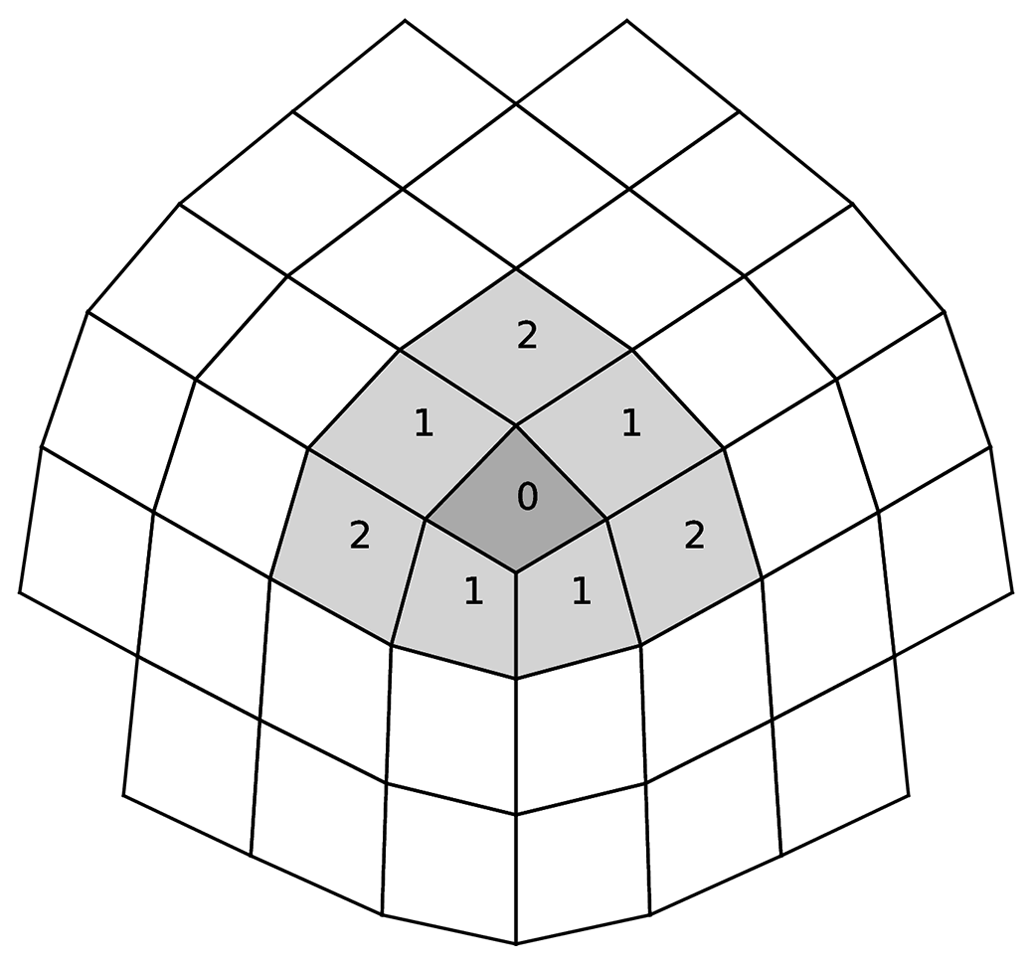
Figure 2 Stencil for a quadratic reconstruction of a field around the corner of a cubed sphere. Numbers indicate at which iteration of the stencil generation the cell is added, lightly shaded cells indicate cells used for the reconstruction that are fitted in a least squares manner, and the darkly shaded cell indicates the central cell which is fitted exactly.

For example, with a quadratic reconstruction n=2 there are n_m=6 monomials, and the stencil algorithm will generate a stencil with n_s=9 cells in general and n_s=8 cells near the corners of the cubed sphere. As in Thuburn et al. (2014) the central cell (k=1) in the stencil is fitted exactly (r₁=0 in Eq. 19), and the others are fitted in a least squares sense.

The local Cartesian coordinates (x,y) are computed as in Thuburn et al. (2014), the origin of the coordinate system x₀ is taken to be the centre of the cell in the centre of the stencil, and the direction of the x axis is then taken as the direction from x₀ to an arbitrary neighbour. Then it is straightforward to reconstruct any point ${\mathit{x}}_i\equiv \left(X_i,Y_i,Z_i\right)$ in the stencil in terms of the local coordinates (x_i,y_i); see Thuburn et al. (2014) for more details.

4.2 Flux computation

Once the scalar field s has been reconstructed at the locations of the 𝕍₁ degrees of freedom to give $\stackrel{\mathrm{ˇ}}{s}$, the flux of that field on a cell face is obtained by multiplying the reconstructed scalar by the normal component of the velocity field at that point:

$$\begin{array}{}\text{(20)}& \widehat{\mathcal{F}}=\widehat{\mathit{u}}\stackrel{\mathrm{ˇ}}{\mathbf{s}},\end{array}$$

where $\stackrel{\mathrm{ˇ}}{\mathbf{s}}$ is the vector containing all $\stackrel{\mathrm{ˇ}}{s}$ at cell edges.

4.3 Predictors

The temporal discretisation is designed to mimic a semi-implicit semi-Lagrangian discretisation such as that used in Wood et al. (2014). For the transport scheme this includes advecting predictors (Φ^p,q^p) for the geopotential and potential vorticity fields instead of the values at the start of the time step (Φⁿ,qⁿ). This is motivated by considering a semi-Lagrangian discretisation of a prototypical equation

$$\begin{array}{}\text{(21)}& {\displaystyle \frac{\mathrm{D}s}{\mathrm{D}t}}+G\left(s\right)=\mathrm{0},\end{array}$$

with $\mathrm{D}/\mathrm{D}t\equiv \partial /\partial t+\mathit{u}\cdot \mathrm{\nabla }$. Discretising across a trajectory from x_D at time level n to x_A at time level n+1 gives

$$\begin{array}{}\text{(22)}& {\left[s+\mathit{\alpha }\mathrm{\Delta }tG\left(s\right)\right]}_{\mathrm{A}}^{n+\mathrm{1}}={\left[s-\left(\mathrm{1}-\mathit{\alpha }\right)\mathrm{\Delta }tG\left(s\right)\right]}_{\mathrm{D}}^n,\end{array}$$

with subscripts “A” and “D” denoting evaluation at arrival x_A and departure x_D points respectively. Evaluation of a function F at a departure point can be expressed as

$$\begin{array}{}\text{(23)}& F_{\mathrm{D}}^n=F_{\mathrm{A}}^n-{\mathcal{A}}_{\mathrm{sl}}\left(F^n,{\stackrel{\mathrm{‾}}{\mathit{u}}}^{\mathrm{1}/\mathrm{2}}\right),\end{array}$$

where 𝒜_sl is the operation of the semi-Lagrangian advection operator. Applying this approximation to Eq. (21) gives

$$\begin{array}{}\text{(24)}& {\displaystyle }{\left[s+\mathit{\alpha }\mathrm{\Delta }tG\left(s\right)\right]}^{n+\mathrm{1}}=s^p-{\mathcal{A}}_{\mathrm{sl}}\left[s^p,{\stackrel{\mathrm{‾}}{\mathit{u}}}^{\mathrm{1}/\mathrm{2}}\right],\text{(25)}& {\displaystyle }{s}^p\equiv {\left[s-\left(\mathrm{1}-\mathit{\alpha }\right)\mathrm{\Delta }tG\left(s\right)\right]}^n,\end{array}$$

where the subscript “A” has been dropped for convenience. Applying this idea to Eq. (2), the geopotential predictor to be advected is then

$$\begin{array}{}\text{(26)}& {\mathrm{\Phi }}^p\equiv {\left[\mathrm{\Phi }-\left(\mathrm{1}-\mathit{\alpha }\right)\mathrm{\Delta }t\mathrm{\Phi }\mathrm{\nabla }\cdot \mathit{u}\right]}^n.\end{array}$$

This can also be applied to potential vorticity using Eq. (4). These predictors come from considering the continuity and PV equations in advective form $\mathrm{D}s/\mathrm{D}t+s\mathrm{\nabla }\cdot \mathit{u}=\mathrm{0}$, where s=Φ or qΦ, as would be used in a semi-Lagrangian model.

5 Solution procedure

The procedure for the solution of the shallow-water equations is as follows. The semi-implicit governing equations, Eqs. (5) and (6), are repeated here for clarity:

$$\begin{array}{}\text{(27)}& {\displaystyle }{\mathit{\delta }}_t\mathit{u}+{\mathcal{F}}^{⟂}\left(q^n{\mathrm{\Phi }}^n,{\stackrel{\mathrm{‾}}{\mathit{u}}}^{\mathrm{1}/\mathrm{2}}\right)+\mathrm{\nabla }{\stackrel{\mathrm{‾}}{\left(K+\mathrm{\Phi }+{\mathrm{\Phi }}_{\mathrm{s}}\right)}}^{\mathit{\alpha }}& {\displaystyle }=\mathrm{0},\text{(28)}& {\displaystyle }{\mathit{\delta }}_t\mathrm{\Phi }+\mathrm{\nabla }\cdot \mathcal{F}\left({\mathrm{\Phi }}^n,{\stackrel{\mathrm{‾}}{\mathit{u}}}^{\mathrm{1}/\mathrm{2}}\right)& {\displaystyle }=\mathrm{0}.\end{array}$$

An iterated implicit scheme is used to solve Eqs. (27) and (28). At each stage (k) of the iterative scheme, the time-level n+1 terms are lagged and included in the residuals such that

$$\begin{array}{}\text{(29)}& {\displaystyle }\begin{array}{rl}{\mathit{R}}_u& \equiv {\left(\mathit{u}+\mathit{\alpha }\mathrm{\Delta }t\mathrm{\nabla }(K+\mathrm{\Phi }+{\mathrm{\Phi }}_{\mathrm{s}})\right)}^{\left(k\right)}\\ & -{\left(\mathit{u}-\left[\mathrm{1}-\mathit{\alpha }\right]\mathrm{\Delta }t\mathrm{\nabla }(K+\mathrm{\Phi }+{\mathrm{\Phi }}_{\mathrm{s}})\right)}^n\\ & +\mathrm{\Delta }t{\mathcal{F}}^{⟂}\left((q\mathrm{\Phi }{)}^p,{\stackrel{\mathrm{‾}}{\mathit{u}}}^{\mathrm{1}/\mathrm{2}}\right),\end{array}\text{(30)}& {\displaystyle }{R}_{\mathrm{\Phi }}\equiv {\mathrm{\Phi }}^{\left(k\right)}-{\mathrm{\Phi }}^n+\mathrm{\Delta }t\mathrm{\nabla }\cdot \mathcal{F}\left({\mathrm{\Phi }}^p,{\stackrel{\mathrm{‾}}{\mathit{u}}}^{\mathrm{1}/\mathrm{2}}\right),\end{array}$$

where k is the estimate for the n+1 terms after k iterations of the iterative scheme. Increments ${\mathit{u}}^{\prime }\equiv {\mathit{u}}^{\left(k+\mathrm{1}\right)}-{\mathit{u}}^{\left(k\right)}$ and ${\mathrm{\Phi }}^{\prime }\equiv {\mathrm{\Phi }}^{\left(k+\mathrm{1}\right)}-{\mathrm{\Phi }}^{\left(k\right)}$ to Eqs. (29)–(30) are sought such that the fast-wave terms are handled implicitly:

$$\begin{array}{}\text{(31)}& {\displaystyle }{\mathit{u}}^{\prime }+\mathit{\tau }f({\mathit{u}}^{\prime }{)}^{⟂}+\mathit{\tau }\mathrm{\Delta }t\mathrm{\nabla }{\mathrm{\Phi }}^{\prime }& {\displaystyle }=-{\mathit{R}}_u,\text{(32)}& {\displaystyle }{\mathrm{\Phi }}^{\prime }+\mathit{\tau }\mathrm{\Delta }t\mathrm{\nabla }\cdot \left({\mathrm{\Phi }}^{*}{\mathit{u}}^{\prime }\right)& {\displaystyle }=-R_{\mathit{\varphi }},\end{array}$$

where Φ^* is a reference state used to obtain the linearisation and τ is a relaxation parameter (usually chosen to be $\mathit{\tau }=\mathrm{1}/\mathrm{2}$). In practice, we use ${\mathrm{\Phi }}^{*}={\mathrm{\Phi }}^n$ as the reference state. Applying the mixed finite-element discretisation, this becomes the system

$$\begin{array}{}\text{(33)}& \left(\begin{array}{cc}{\mathbf{M}}_{\mathrm{1}}+\mathit{\tau }\mathrm{\Delta }t\mathbf{C}& -\mathit{\tau }\mathrm{\Delta }t\mathbf{D}{\left(\mathrm{1}\cdot \right)}^T\\ \mathit{\tau }\mathrm{\Delta }t\mathbf{D}\left({\mathrm{\Phi }}^{*}\cdot \right)& {\mathbf{M}}_{\mathrm{2}}\end{array}\right)\left(\begin{array}{c}{\mathit{u}}^{\prime }\\ {\mathrm{\Phi }}^{\prime }\end{array}\right)=-\left(\begin{array}{c}{\mathcal{R}}_u\\ {\mathcal{R}}_{\mathrm{\Phi }}\end{array}\right),\end{array}$$

where 𝓡_u and ℛ_Φ are the finite-element discretisations of Eqs. (29) and (30) respectively given by Eqs. (11) and (12). The matrices are defined as

$$\begin{array}{}\text{(34)}& {\displaystyle }{\mathbf{M}}_{\mathrm{1}}^{i,j}\equiv & {\displaystyle }\underset{\mathbf{D}}{\int }\mathbf{J}{\widehat{\mathit{w}}}_i\cdot {\displaystyle \frac{\mathbf{J}}{\text{det}\mathbf{J}}}{\widehat{\mathit{w}}}_j\mathrm{d}\widehat{A},\text{(35)}& {\displaystyle }{\mathbf{M}}_{\mathrm{2}}^{i,j}\equiv & {\displaystyle }\underset{\mathbf{D}}{\int }{\widehat{\mathit{\sigma }}}_i{\widehat{\mathit{\sigma }}}_j\text{det}\mathbf{J}\mathrm{d}\widehat{A},\text{(36)}& {\displaystyle }{\mathbf{C}}^{i,j}\equiv & {\displaystyle }f\underset{\mathrm{D}}{\int }\mathbf{J}{\widehat{\mathit{w}}}_i\cdot {\displaystyle \frac{\mathbf{J}}{\text{det}\mathbf{J}}}{\widehat{\mathit{w}}}_j^{⟂}\mathrm{d}\widehat{A},\text{(37)}& {\displaystyle }\mathbf{D}{\left(\mathit{\psi }\right)}^{i,j}\equiv & {\displaystyle }\underset{\mathbf{D}}{\int }\widehat{\mathrm{\nabla }}\cdot {\widehat{\mathit{w}}}_i\mathit{\psi }{\mathit{\sigma }}_j\mathrm{d}\widehat{A}.\end{array}$$

At each iteration (k) the system (33) is solved using an iterative Krylov subspace method (in this case the generalised minimal residual method – GMRES). For the tests presented in this paper (see Sect. 7), GMRES generally converged in two to three iterations to a tolerance of 10⁻⁴.

6 Mesh

An equiangular cubed sphere mesh is used to grid the sphere. We use the notation Cn to describe a cubed sphere with n×n cells per panel. The mesh is parameterised using a finite-element representation of the sphere within a cell with polynomials of order m. Note therefore that a point within a cell does not necessarily lie on the sphere, with the error depending on the order of the elements used. For example, a linear element lies on the sphere at the vertices of the element and uses a linear approximation to the surface of the sphere within the element. Representing the sphere with these elements removes the need for analytical transforms to the reference grid, allowing the use of an arbitrary grid if required (in this paper we use the standard equiangular cubed sphere). To compute the error of the mesh parameterisation, the geocentric coordinates $(X,Y,Z)$ at a point in the cell are computed using the finite-element representation. The error is the difference between the true radius of the sphere and the radius using $(X^{\mathrm{2}}+Y^{\mathrm{2}}+Z^{\mathrm{2}}{)}^{\mathrm{1}/\mathrm{2}}$.

Figure 3 shows the error within a cell when using linear and quadratic elements on a C96 grid with the Earth's radius. The error for the linear element is largest at the cell centre, with a maximum error of 426.39 m. The quadratic element reduces the error by 5 orders of magnitude, with a maximum error of 0.0018 m. Figure 3c shows the convergence of the maximum error within a cell. The linear element error converges at second order, with the quadratic element converging at fourth order. For this reason the quadratic element is used to create the mesh for the shallow-water model. Note that the quadratic element is for the representation of the mesh, whereas the lowest-order finite elements are used for the spatial discretisation of the model.

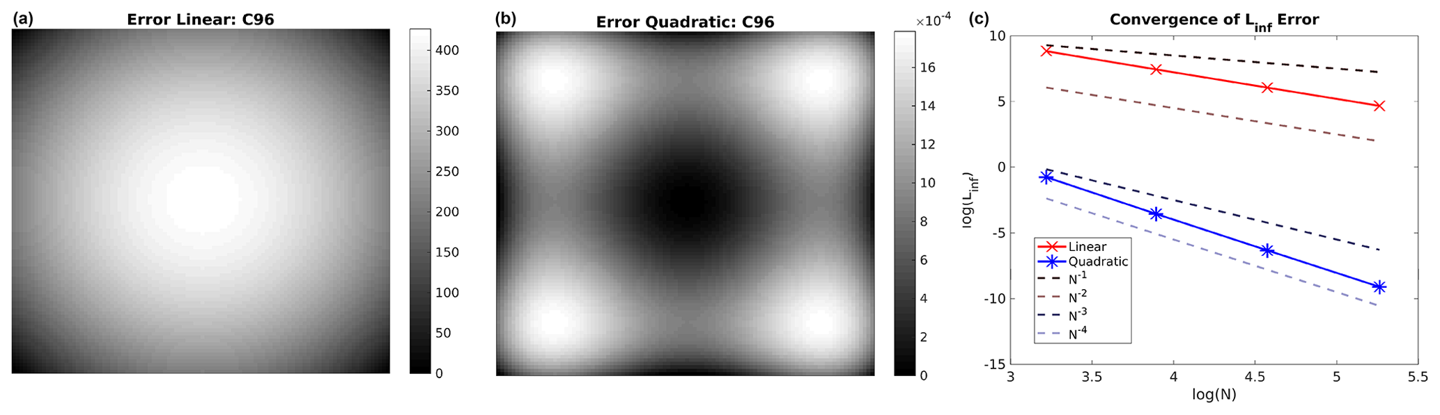
Figure 3 The error from linear and quadratic finite-element representations of the sphere within a cell. The left and centre plots show the absolute error (true – FE) for the linear and quadratic basis functions respectively on the C96 cubed sphere grid. The right plot shows the convergence of the ℓ_inf error, using C24, C48, C96 and C192 cubed sphere grids.

7 Numerical results

This section shows the results of the model runs using a standard set of spherical shallow-water test cases. The full initial conditions for each of the tests are given in the references under each test case.

7.1 Williamson 2: steady state

The first test case is the steady-state test described in Williamson et al. (1992). The steady flow means that the initial conditions are the analytical solution at any time, and thus error norms can be calculated for the runs at different resolutions.

The normalised ℓ₂ error norms of the geopotential field at 15 d are given in the top two rows of Table 1 for the C24 (Δt=3600), C48 (Δt=1800), and C96 (Δt=900) resolutions. The error norms can be used to determine the convergence rate and hence the empirical order of accuracy of the model. The convergence rates of the ℓ₂ and ℓ_∞ error norms are approximately second order. This is expected as the finite-element discretisation and the time-stepping scheme are both second-order methods. The error fields after 15 d for the C96 resolution are shown in Fig. 4: these errors show a wave number 4 pattern coming from the underlying cubed sphere mesh; however, the errors are large scale and are not particularly clustered around the edges and corners of the cubed sphere, indicating an acceptable level of grid imprinting.

Table 1 The normalised ℓ₂ and ℓ_∞ geopotential error norms for the Williamson 2 test (top) and the normalised ℓ₂ and absolute ℓ_∞ geopotential error norms for the Williamson 5 test (bottom) at different resolutions after 15 d.

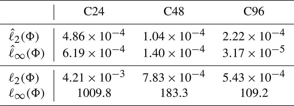
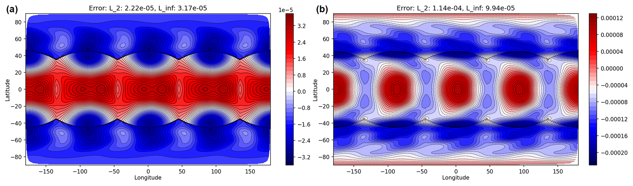
Figure 4 Errors after 15 d for the Williamson 2 test at C96 resolution for geopotential (a) and zonal wind (b) showing the large-scale nature of the error.

7.2 Williamson 5: mountain test

The mountain test case of Williamson et al. (1992) is used to show the performance of the model when orography is present (i.e. Φ_s≠0). The initial zonal flow is over a mountain centred at 90^∘ longitude and 30^∘ latitude. The same grid resolutions and time steps used for the Williamson 2 test are used for the mountain test.

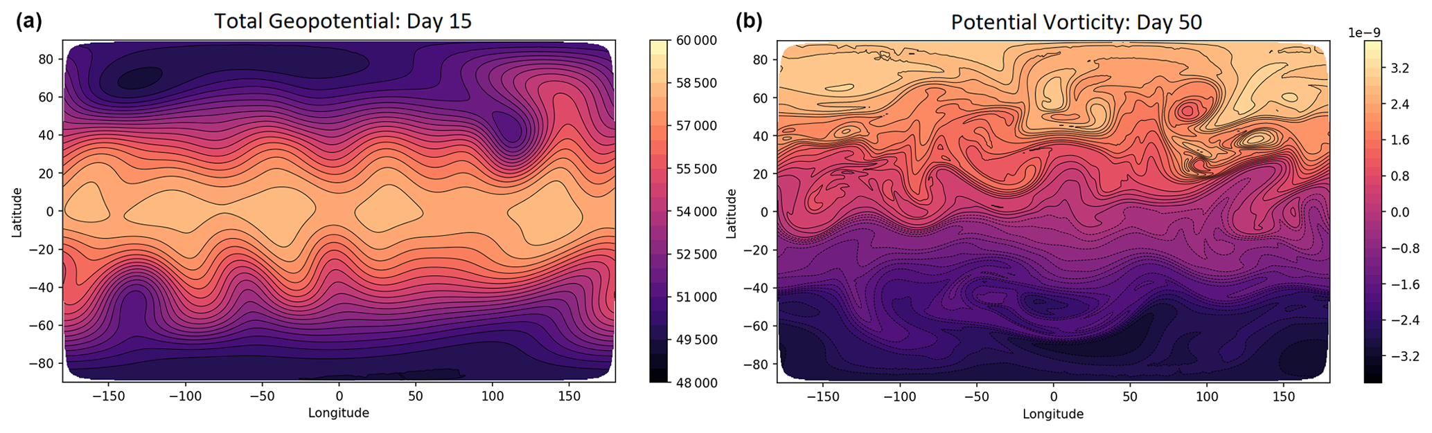
Figure 5 Results for the Williamson mountain test on the C96 grid. Panel (a) shows the total geopotential (Φ+Φ_s) after 15 d. Panel (b) shows the potential vorticity (q) after 50 d.

The geopotential at day 15, shown in Fig. 5a for the C96 grid, is comparable to other shallow-water models at similar resolutions (see for example Thuburn et al., 2010, 2014; Ullrich, 2014). We investigate the errors in the total geopotential by comparing them with a high-resolution solution generated using the semi-implicit semi-Lagrangian (SISL) shallow-water model of Zerroukat et al. (2009). This reference solution uses a time step of Δt=60 s and a high-resolution latitude–longitude grid of 1536×768 points. The high-resolution solution is then interpolated, using bi-cubic interpolation, to the corresponding cubed sphere grid where the difference is taken to produce the error plots and diagnostics.

Figure 6 Absolute error plots for total geopotential (Φ+Φ_s) for the Williamson mountain test on the C24 grid (a) and the C48 grid (b) after 15 d. Note the different scales on the colour bars.

The error plots for the total geopotential are shown in Fig. 6 for the C24 and C48 resolutions. The error for the C48 solution is visually similar to that of the finite-element cubed sphere model of Thuburn and Cotter (2015) (their Fig. 7), with a large negative error near the mountain and the wave train error in the Southern Hemisphere. The errors decrease significantly as the resolution increases. The normalised ℓ₂ and absolute ℓ_∞ error norms, calculated from the high-resolution SISL model, are given in the bottom of Table 1.

The C48 maximum errors (given in Fig. 6 and in Table 1) are smaller in magnitude than those for the 13 824-cell finite-volume cubed sphere model of Thuburn et al. (2014) and have a similar magnitude to the SISL model (Zerroukat et al., 2009) at 160×80 resolution (note that Thuburn et al., 2014, use total height, not total geopotential, in their results, and so their results need to be multiplied by gravity to give an equivalent value). The absolute ℓ_∞ error norm values converge at a rate of 1.6, similarly to those given in Thuburn et al. (2014) (note that they use a smaller time step than presented in our results).

The normalised ℓ₂ errors of the geopotential, given in the bottom of Table 1, have a convergence rate of 2.42 between C24 and C48. However, at higher resolution the error convergence stalls, similarly to that found in Thuburn et al. (2014) for comparable time steps, with a rate of only 0.53 between C48 and C96. Even with this stalling, the total rate between C24 and C96 is 1.48.

To demonstrate the conservation properties of the model, the mass, total energy and potential enstrophy are computed at each time step. The total energy is defined as

$$\begin{array}{}\text{(38)}& E=\underset{\mathrm{D}}{\int }{\displaystyle \frac{\mathrm{1}}{\mathrm{2}}}h\left(|\mathit{u}{|}^{\mathrm{2}}+\mathrm{\Phi }+\mathrm{2}{\mathrm{\Phi }}_{\mathrm{s}}\right)\mathrm{d}A,\end{array}$$

and the potential enstrophy is defined as

$$\begin{array}{}\text{(39)}& Z=\underset{\mathrm{D}}{\int }{\displaystyle \frac{\mathrm{1}}{\mathrm{2}}}\mathrm{\Phi }{q}^{\mathrm{2}}\mathrm{d}A,\end{array}$$

where the integrals are over the whole domain.

Mass, energy, and potential enstrophy are conserved in the continuous equations. As the model uses a finite-volume transport scheme, the mass is conserved to machine precision; however, energy and potential enstrophy are not conserved by the discretisation presented here, and in fact, in the discrete case, potential enstrophy cascades downscale from resolved to unresolved scales and thus is expected to decrease with time.

The normalised total energy and potential enstrophy are plotted against time in Fig. 7 for different grid resolutions (C24, C48, and C96) up to day 50. As the resolution increases, the dissipation in the model decreases, and the total energy and potential enstrophy curves are closer to conservation (a horizontal line). The flow is initially weakly non-linear, and so for the first 15 d there are no significant cascades to unresolved scales. After 15 d the percentage loss in total energy is 0.0355 % for C24, 0.0062 % for C48, and 0.001 % for C96. For potential enstrophy the percentage loss is 0.3648 % for C24, 0.076 % for C48, and 0.014 % for C96. Extending to 50 d, the flow becomes more non-linear, and this results in more dissipation of energy and potential enstrophy. The percentage losses are 0.221 % for C24, 0.063 % for C48, and 0.014 % for C96 in the total energy and 3.33 % for C24, 2.19 % for C48, and 1.45 % for C96 in the potential enstrophy.

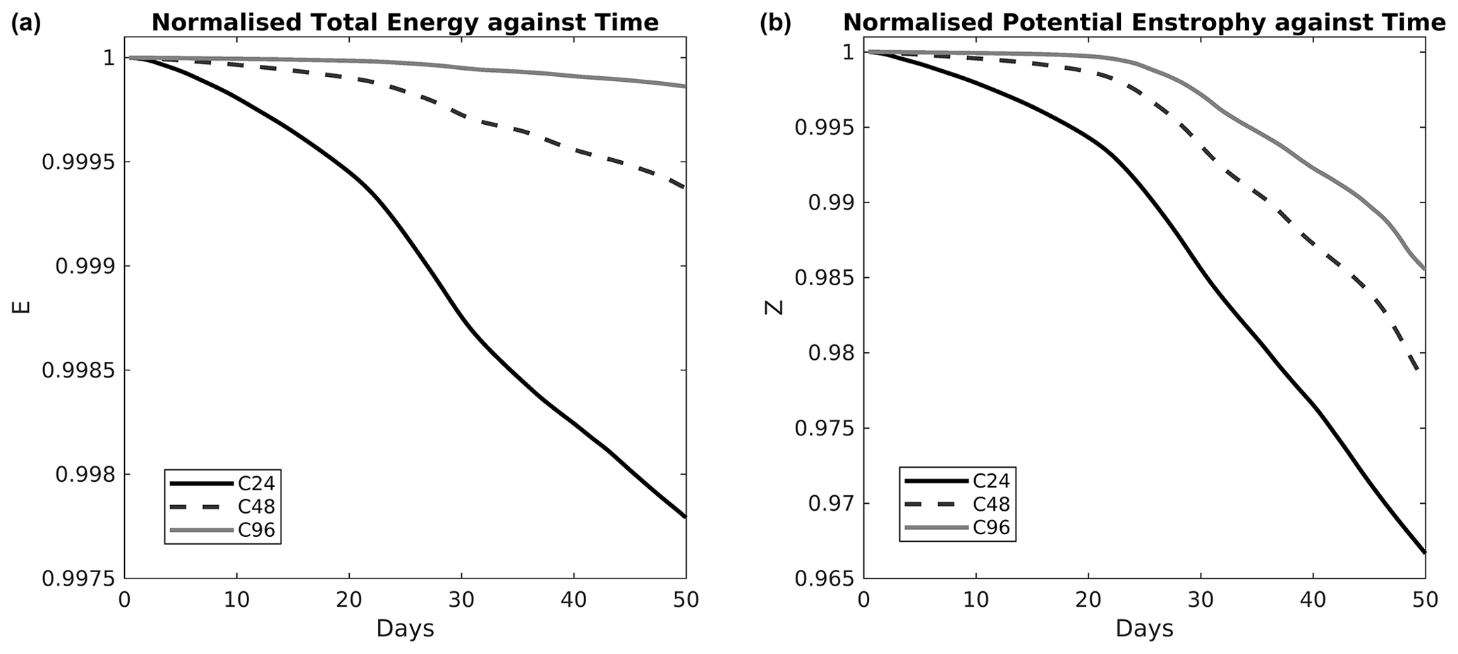
Figure 7 The normalised total energy (a) and potential enstrophy (b) against time for the Williamson mountain test.

The potential vorticity at day 50 is shown in Fig. 5b for the C96 resolution. As the flow has become non-linear, the potential vorticity contours start to wrap up. The model captures the potential vorticity filaments without producing noise. The results for this test indicate that the model is correctly simulating flow over orography.

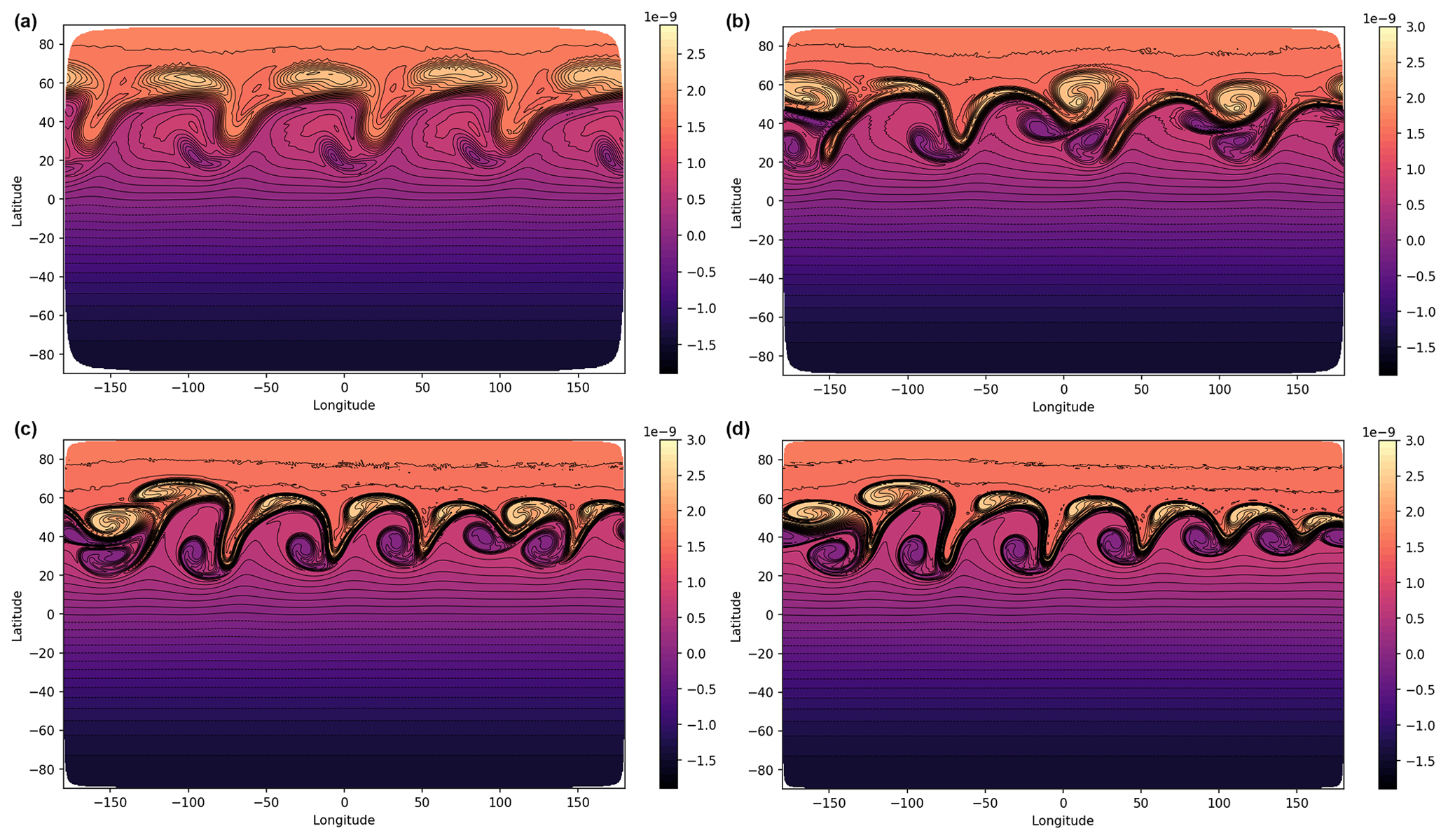
Figure 8 The potential vorticity q after 6 d for the Galewsky instability test. Panel (a) shows the C48 solution, panel (b) shows the C96 solution, panel (c) shows the C192 solution, and panel (d) shows the C384 solution.

7.3 Galewsky instability test

For the Galewsky instability test (Galewsky et al., 2004), a perturbation is added to a balanced jet to create a barotropic instability. As the instability progresses, many small-scale potential vorticity filaments are produced.

The potential vorticity solutions at day 6 are shown in Fig. 8 for the C48, C96, C192, and C384 resolution runs (with Δt=900, 450, 225, and 112.5 s respectively). At C48 resolution the grid imprinting from the cubed sphere is evident. A wave number 4 pattern appears on the jet, dominating the development of the instability. Increasing the resolution to C96, C192, or C384 reduces the impact of the grid imprinting; however, the instability has still developed more than in the reference solution of Galewsky et al. (2004) at T341 resolution. This is consistent with the finite-element cubed sphere model of Thuburn and Cotter (2015), which uses a similar mixed finite-element discretisation to the one used here. In Thuburn and Cotter (2015) it is stated that the grid imprinting may be exaggerated by the highly unstable initial state of this test.

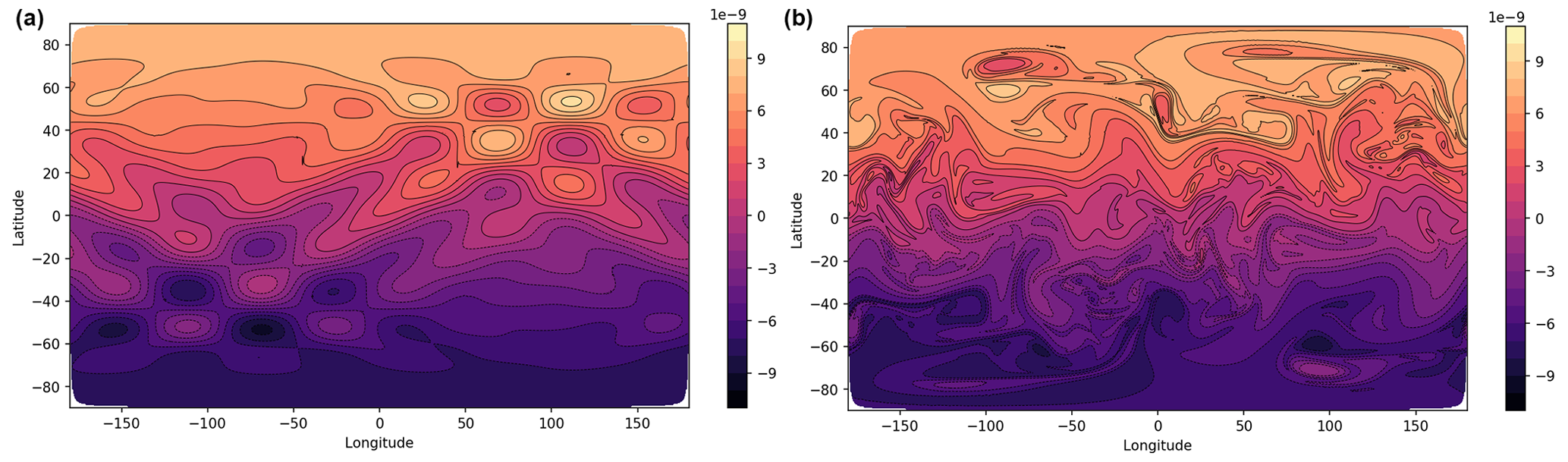
Figure 9 The potential vorticity q for the vortices test case. Panel (a) shows the initial conditions, and panel (b) shows the solution after 15 d from a high-resolution C192 simulation.

At the higher resolution many small-scale features are resolved by the model without producing grid-scale noise. This is due to the implicit diffusion from the transport scheme damping grid-scale features. These solutions are comparable to the results shown in Thuburn et al. (2014) and Thuburn and Cotter (2015).

Figure 10 The potential vorticity q for the vortices test case after 15 d for the C24 resolution (a) and the C96 resolution (b).

7.4 Vortices test

The final test case is the field of vortices test from Kent et al. (2016). A field of vortices (shown by the potential vorticity in Fig. 9a) is set to evolve over a number of days. The vortices interact, leading to small-scale vorticity filaments and fingers as the vortices are stretched out as well as the merger of vortices. A high-resolution run (using C192 resolution, with potential vorticity shown after 15 d in Fig. 9b) is used as a reference solution.

Figure 10 shows the day 15 potential vorticity for the C24 and C96 runs (with Δt=1800 and 450 s respectively). The C24 run is unable to resolve many of the features of the vortices, but the implicit diffusion from the transport scheme is sufficient to prevent grid-scale noise. For the higher-resolution C96 run, the small-scale features of the potential vorticity are well represented, and the solution matches the reference solution well. This demonstrates the model's ability to represent small-scale features without producing grid-scale noise.

8 Conclusions

This article presents a new shallow-water model on the sphere. The model is comprised of a mixed finite-element spatial discretisation, a high-order finite-volume transport scheme, and an iterated semi-implicit time scheme and makes use of the cubed sphere grid. The finite-element discretisation is chosen as it has been shown to be both accurate and scalable on many processors (Cotter and Shipton, 2012). The lowest-order finite-element method is used to give second-order spatial accuracy, and the finite-element spaces are such that they are analogous to a C-grid staggering. The semi-implicit time stepping provides stability for the fast gravity waves along with second-order temporal accuracy. The method-of-lines advection scheme, using third-order Runge–Kutta time stepping with a quadratic finite-volume reconstruction, gives high accuracy and conservation for transport.

The model achieves computational efficiency through the use of the mixed finite-element method and the cubed sphere grid. The cubed sphere cells are more uniform in size than the traditional latitude–longitude grid, and so fewer cells are required for the same resolution. For example, a 1^∘ × 1^∘-resolution grid requires $\mathrm{360}\times \mathrm{180}=\mathrm{64}\mathrm{800}$ cells on a latitude–longitude grid but only 48 600 cells on a C90 cubed sphere grid (with both grids having 360 cells around the Equator). The cubed sphere grid also removes the pole problem of the latitude–longitude grid and thus is more scalable on massively parallel architecture (Staniforth and Thuburn, 2012).

The model has been tested on a standard set of shallow-water test cases. The Williamson steady-state test shows that the model converges at second-order accuracy. The mountain test demonstrates the model's ability to capture flow over orography. Grid imprinting from the Galewsky instability test is evident at coarse spatial resolutions but is significantly reduced at higher resolutions, in line with results from other models with similar discretisations and cubed sphere meshes. The vortex field test highlights that the model can resolve small-scale features without producing grid-scale noise. The results presented from this testing are comparable to other models in the literature. This indicates that this model has a similar level of accuracy to these other well-known shallow-water models.

This shallow-water model has been developed alongside the mixed finite-element Cartesian model for atmospheric dynamics of Melvin et al. (2019). The vector-invariant model presented here is a building block towards a mixed finite-element spherical geometry dynamical core for the atmosphere.