Simulating marine neodymium isotope distributions using Nd v1.0 coupled to the ocean component of the FAMOUS–MOSES1 climate model: sensitivities to reversible scavenging efficiency and benthic source distributions

The neodymium (Nd) isotopic composition of seawater is a widely used ocean circulation tracer. However, uncertainty in quantifying the global ocean Nd budget, particularly constraining elusive non-conservative processes, remains a major challenge. A substantial increase in modern seawater Nd measurements from the GEOTRACES programme, coupled with recent hypotheses that a seafloor-wide benthic Nd flux to the ocean may govern global Nd isotope distributions (ε_Nd), presents an opportunity to develop a new scheme specifically designed to test these paradigms. Here, we present the implementation of Nd isotopes (¹⁴³Nd and ¹⁴⁴Nd) into the ocean component of the FAMOUS coupled atmosphere–ocean general circulation model (Nd v1.0), a tool which can be widely used for simulating complex feedbacks between different Earth system processes on decadal to multi-millennial timescales.

Using an equilibrium pre-industrial simulation tuned to represent the large-scale Atlantic Ocean circulation, we perform a series of sensitivity tests evaluating the new Nd isotope scheme. We investigate how Nd source and sink and cycling parameters govern global marine ε_Nd distributions and provide an updated compilation of 6048 Nd concentrations and 3278 ε_Nd measurements to assess model performance. Our findings support the notions that reversible scavenging is a key process for enhancing the Atlantic–Pacific basinal ε_Nd gradient and is capable of driving the observed increase in Nd concentration along the global circulation pathway. A benthic flux represents a major source of Nd to the deep ocean. However, model–data disparities in the North Pacific highlight that under a uniform benthic flux, the source of ε_Nd from seafloor sediments is too non-radiogenic in our model to be able to accurately represent seawater measurements. Additionally, model–data mismatch in the northern North Atlantic alludes to the possibility of preferential contributions from “reactive” non-radiogenic detrital sediments.

The new Nd isotope scheme forms an excellent tool for exploring global marine Nd cycling and the interplay between climatic and oceanographic conditions under both modern and palaeoceanographic contexts.

1 Introduction

The neodymium (Nd) isotope composition of seawater shows a clear provinciality between different ocean basins and is often used as a water mass provenance tracer (e.g. Frank, 2002; Goldstein and Hemming, 2003). The measured ${}^{\mathrm{143}}\mathrm{Nd}{/}^{\mathrm{144}}\mathrm{Nd}$ ratio is denoted relative to the bulk Earth standard:

$$\begin{array}{}\text{(1)}& {\mathit{\epsilon }}_{\mathrm{Nd}}=\left({\displaystyle \frac{{\left({}^{\mathrm{143}}\mathrm{Nd}{/}^{\mathrm{144}}\mathrm{Nd}\right)}_{\mathrm{sample}}}{{\left({}^{\mathrm{143}}\mathrm{Nd}{/}^{\mathrm{144}}\mathrm{Nd}\right)}_{\mathrm{CHUR}}}}-\mathrm{1}\right)\times {\mathrm{10}}^{\mathrm{4}},\end{array}$$

where (${}^{\mathrm{143}}\mathrm{Nd}{/}^{\mathrm{144}}\mathrm{Nd}$)_CHUR relates to the Chondritic Uniform Reservoir (CHUR; 0.512638: Jacobsen and Wasserburg, 1980). Distinct variations in the Nd isotope signal of water masses originate from different continental regions and their isotopic fingerprints and subsequent influence by ocean circulation, water mass mixing, and particle cycling, as well as interaction with sediments (e.g. Tachikawa et al., 2017; van de Flierdt et al., 2016 for recent reviews). Neodymium in the deep ocean has an estimated mean ocean residence time between 360 and 800 years (Arsouze et al., 2009; Rempfer et al., 2011; Gu et al., 2019; Pöppelmeier et al., 2020a, 2021b), which is shorter than the global overturning of the deep ocean. Unlike other tracers of ocean circulation (e.g. δ¹³C, Δ¹⁴C), Nd is not fractionated by marine biological cycling, giving rise to its promise as a carbon-cycle-independent ocean circulation tracer (Blaser et al., 2019a). Yet, a fundamental caveat in the application of ε_Nd as a reliable oceanographic tracer is that knowledge of the Nd fluxes in and out of the ocean remains incomplete, and while internal cycling must occur, the efficiency of it with different particle types is poorly constrained (Abbott et al., 2015a; Haley et al., 2017; van de Flierdt et al., 2016).

Numerical models are useful tools for investigating Nd cycling since they can specify the processes that govern the spatiotemporal variability in Nd isotope distributions in the ocean. Neodymium isotopes have been simulated in a range of different modelling studies testing specific hypotheses relating to Nd fluxes and thermohaline redistribution (Pöppelmeier et al., 2020a; Arsouze et al., 2009; Rempfer et al., 2011; Siddall et al., 2008; Jones et al., 2008; Roberts et al., 2010; Tachikawa et al., 2003; Ayache et al., 2016; Gu et al., 2019; Oka et al., 2021, 2009; Pöppelmeier et al., 2022; Ayache et al., 2023; Pasquier et al., 2022; Du et al., 2020). However, recent work suggests that a seafloor-wide benthic flux, resulting from early diagenetic reactions, may dominate the marine Nd cycle (Haley et al., 2017; Abbott, 2019; Abbott et al., 2015a, b, 2019; Du et al., 2016). These observations, alongside an ever-growing body of high-quality and highly resolved measurements of dissolved seawater Nd concentrations ([Nd]) and ε_Nd from the GEOTRACES programme (GEOTRACES Intermediate Data Product Group, 2021), present an opportunity to re-evaluate, revise, and explore constraints on the marine Nd cycle.

Initially, the predominant lithogenic fluxes of Nd to the ocean were believed to be mostly at the surface (aeolian dust and riverine fluxes; Goldstein et al., 1984; Goldstein and Jacobsen, 1987). Early modelling studies applying surface fluxes reproduced reasonable ε_Nd in the North Atlantic (Bertram and Elderfield, 1993; Tachikawa et al., 1999). However, considering only dust and river fluxes alone led to an unrealistic calculated residence time of Nd in seawater on the order of 5000 years (Bertram and Elderfield, 1993; Jeandel et al., 1995). It was then found that considering dust and river surface inputs alone failed to balance both [Nd] and ε_Nd, thus indicating a “missing source” of Nd to the ocean that accounted for ≈90 % of the Nd flux to the ocean (Tachikawa et al., 2003). This led to a new hypothesis relating to other Nd sources to seawater that could account for this missing source, including submarine groundwater discharge (SGD) (Johannesson and Burdige, 2007) and exchange of Nd between seawater and sediment deposited on the continental margins (Lacan and Jeandel, 2005). The term “boundary exchange” was then coined to describe significant modification of Nd isotopic composition by the co-occurrence of Nd release from sediment and boundary scavenging without substantially changing [Nd] (Lacan and Jeandel, 2005). Arsouze et al. (2007) simulated realistic global ε_Nd distributions using sedimentary fluxes constrained to the continental margins as the only source–sink term, and since then particle–seawater exchange along the margins has represented the major flux of Nd to seawater in recent global Nd isotope models (Arsouze et al., 2009; Rempfer et al., 2011; Gu et al., 2019).

Nonetheless, seafloor–sediment interactions along the continental margins alone cannot fully reconcile the global marine Nd cycle. Specifically, it cannot explain the observed vertical profiles of [Nd], which are decoupled from ε_Nd (i.e. the “Nd paradox”; Goldstein and Hemming, 2003), with low concentrations near the surface increasing with depth. This is a common characteristic of isotopes and elements (e.g. thorium) that are reversibly scavenged (i.e. where the element is scavenged onto sinking particles at the surface and is subsequently remineralised in the deep ocean) (Bertram and Elderfield, 1993; Bacon and Anderson, 1982). Siddall et al. (2008) first addressed a numerical hypothesis that the Nd paradox can be explained by a combination of lateral advection and reversible scavenging by applying the reversible scavenging model pioneered by Bacon and Anderson (1982) to Nd cycling. In their study, both [Nd] and ε_Nd were modelled simultaneously and explicitly to explore internal cycling of Nd in the deep ocean. Their findings demonstrated that scavenging and remineralisation processes are important active components in the marine cycling of Nd, driving the increase of [Nd] with depth but still allowing ε_Nd to act as an effective water mass tracer.

Although inclusion of reversible scavenging can explain aspects of marine Nd cycling, the use of oversimplified fixed surface [Nd] and ε_Nd boundary conditions in the model by Siddall et al. (2008) limited what could be determined about the full marine cycling of Nd and hence the Nd paradox. The most comprehensive Nd-isotope-enabled ocean models to date now explicitly represent and quantify a wider range of distinct Nd fluxes that are both external and internal to the marine realm. For example, Arsouze et al. (2009) used a fully prognostic coupled dynamic and biogeochemical model to simulate [Nd] and ε_Nd, considering dust fluxes, dissolved riverine sources, sediment sources along the continental margins, and reversible scavenging. In their study, a sediment source from the continental margins represented the major source of Nd to seawater (≈95 % of the total source). Rempfer et al. (2011) continued this work, undertaking a more detailed and comprehensive investigation of Nd sources and particle scavenging using a coarse-resolution intermediate-complexity model (Bern3D ocean model) and extensive sensitivity experiments. This later scheme was then closely followed by Gu et al. (2019) for the implementation of Nd isotopes in the ocean component of a more comprehensive Earth system model (ESM, specifically the Community Earth System Model, CESM1.3) to explore the changes to end-member ε_Nd signatures in response to ocean circulation and climate changes in detail. Overall, these comprehensive models, capable of quantifying the major sources implicated in marine Nd cycling, indicated that dust and river fluxes were important for representing [Nd] and ε_Nd distributions in the surface but that the main flux of Nd to seawater is via a sediment source operating along the continental margins.

Recent pore fluid concentration profiles measured on the Oregon margin in the Pacific Ocean indicate that there may be a benthic flux of Nd from sedimentary pore fluids, presenting a potential major seafloor-wide (i.e. no longer limited to the continental margins) source of Nd to seawater (Abbott et al., 2015b, a); however, there are observations of low [Nd] from southeastern equatorial Pacific pore waters, implying possibly heterogeneous benthic flux in relation to deep-sea sediment composition (Paul et al., 2019). Additional measurements from the Tasman Sea inferred the likely presence of a benthic source of similar magnitude to that estimated for the North Pacific, which may indicate that regions with dominantly calcareous sediment also contribute a significant benthic source of Nd (Abbott, 2019). Evidence of this previously overlooked benthic sedimentary source of Nd has led to a shifting paradigm that contends that the dominant addition of Nd to the ocean is from a diffuse sedimentary source at depth, rather than surface point sources from rivers and dust and the shallow to intermediate continental margins (Haley et al., 2017).

Simple box models have been employed to investigate, to a first order, the non-conservative effects from a benthic flux (Du et al., 2016, 2018, 2020; Haley et al., 2017; Pöppelmeier et al., 2020b), suggesting overprinting of deep-water mass ε_Nd is linked to benthic flux exposure time and the difference between the Nd isotope composition of the benthic flux and the bottom water (Abbott et al., 2015a; Du et al., 2018). However, these models lack comprehensive descriptions of both the marine Nd cycle and of physical ocean circulation and climate interactions, limiting a clear interpretation of precisely how (and under what physical or environmental conditions) the benthic flux may determine global marine Nd distributions. Applying an intermediate complexity model, Pöppelmeier et al. (2021a) investigated the benthic flux hypothesis in more detail by updating the Nd-isotope-enabled Bern3D model (Rempfer et al., 2011) to represent recent observations that indicate a Nd flux from bottom waters could occur across the entire seafloor. This was done by removing the depth limitation of the sediment source (previously 3 km) and invoking a constant benthic flux that escapes from all sediment–water interfaces. The scheme was further extended by revising key source–sink parameterisations for subsequent investigation of non-conservative Nd isotope behaviour under different ocean circulation states (Pöppelmeier et al., 2022). The authors demonstrate substantial non-conservative effects occur even under strong circulation regimes with low benthic flux exposure times and are not strictly limited to the deep ocean. This work highlights the importance of downward vertical fluxes via reversible scavenging alongside the benthic flux to describe non-conservative marine Nd isotope behaviour. Nonetheless, the low horizontal resolution of the intermediate-complexity model limits full resolution of key circulation patterns such as distinct deep-water formation in the Labrador Sea and in the Nordic Seas, inhibiting the capability of the scheme to fully capture and explore water mass end-member ε_Nd distributions.

Thus, despite substantial progress to explicitly describe seawater Nd budgets, it is apparent that outstanding questions remain, alongside divergent lines of argument amongst subject specialists, limiting a full, quantitative description of marine Nd cycling. The decoupled nature of marine [Nd] and ε_Nd, which is yet to be fully understood, and new emerging observations (e.g. Stichel et al., 2020; Lagarde et al., 2020; Paffrath et al., 2021; Deng et al., 2022) emphasise the critical need to progress our understanding of modern marine Nd cycling in the light of continued use of ε_Nd as a valuable tracer of ocean circulation. In this context, Nd-isotope-enabled ocean models remain an effective way to understand seawater measurements and to progress with testing and constraining processes governing marine Nd cycling, which can then feedback key information to the wider GEOTRACES and ocean tracer modelling community.

With this is mind, there is a current gap in the toolkit for modelling marine Nd cycling between the class of high-complexity, state-of-the-art ESMs (e.g. Gu et al., 2019) and the more efficient intermediate-complexity models (e.g. Rempfer et al., 2011; Pöppelmeier et al., 2020a). To bridge this gap, there is a need for a model with the full complexity of an atmosphere–ocean general circulation model (AOGCM), allowing the exploration of how Nd isotopes vary under changing climate conditions (including extensive palaeoceanographic applications), that is also capable of running very quickly to facilitate efficient parameter space exploration, performance optimisation and long integrations. Owing to a winning combination of speed and complexity, the FAMOUS general circulation model (GCM) fills this gap and is well suited to exploring Earth system interactions (Smith et al., 2008; Jones et al., 2005; Smith, 2012; Jones et al., 2008).

Here we present the new global marine Nd isotope scheme (Nd v1.0) implemented in FAMOUS. We utilise the new sediment ε_Nd maps from Robinson et al. (2021) as boundary conditions for a mobile global sediment Nd flux, with the end goal of further constraining the major sources, sinks, and cycling of Nd isotopes and exploring instances of non-conservative behaviour related to changes in Nd source distributions and scavenging processes. We develop sensitivity experiments (Sect. 3) to isolate the physical effects of varying two key parameters that detail major Nd fluxes and cycling to the global ocean, verifying foremost that the new isotope scheme is responding to Nd source and sink and biogeochemical processes as expected and contextualising how and where reversible scavenging processes and the benthic flux can govern marine [Nd] and ε_Nd distributions. Finally (Sects. 3 and 4), we evaluate overall model performance through comparison with modern measurements and assess the model's ability to simulate observed spatial and vertical gradients between ocean basins, encompassing underling structural uncertainty and model bias.

2 Methods

2.1 Model description

We use the FAMOUS GCM (Smith et al., 2008; Jones et al., 2005; Smith, 2012), a fast coupled AOGCM derived from the Met Office's Hadley Centre Coupled Model V3 (HadCM3) AOGCM (Gordon et al., 2000). The atmospheric component of FAMOUS is based on quasi-hydrostatic primitive equations and has a horizontal resolution of 5^∘ latitude by 7.5^∘ longitude, 11 vertical levels on a hybrid sigma-pressure coordinate system and a 1 h time step. The ocean component is a rigid-lid model, with a horizontal resolution of 2.5^∘ latitude by 3.75^∘ longitude and 20 vertical levels, spaced unequally in thickness from 10 m at the near-surface ocean to over 600 m at depth, and a 12 h time step. The ocean and atmosphere are coupled once per day.

FAMOUS's parameterisations of physical and dynamical processes are almost identical to those of HadCM3, its parent model, but it has approximately half the spatial resolution and a longer time step, allowing it to run 10 times faster. Thus, FAMOUS achieves a current speed of up to 650 model years per wall clock day on 16 processors, making it ideal for running large ensembles (Gregoire et al., 2011, 2016), more bespoke sensitivity studies (Smith and Gregory, 2009; Gregoire et al., 2015), and multi-millennial simulations, e.g. to examine ice sheet behaviours (Gregoire et al., 2012, 2016, 2015), ocean drifts (Dentith et al., 2019), and ocean biogeochemistry (Dentith et al., 2020). FAMOUS is calibrated to the performance of HadCM3, taking the philosophy that this is the most appropriate evaluation target and that it is unrealistic to expect the lower-resolution, lower-complexity model to outperform its parent model (Valdes et al., 2017; Smith and Gregory, 2009).

We added Nd isotopes (¹⁴³Nd and ¹⁴⁴Nd) as optional passive tracers into the ocean component of FAMOUS, using a version of the model with the Met Office Surface Exchange Scheme (MOSES) version 1 (Cox et al., 1999: FAMOUS–MOSES1). It was a pragmatic choice to avoid the more recent FAMOUS–MOSES2.2 configuration (Essery and Clark, 2003; Valdes et al., 2017; Williams et al., 2013; Essery et al., 2001) because evaluation of our new Nd scheme would be hindered by the collapsed Atlantic Ocean convection and strong deep Pacific meridional overturning circulation (MOC) produced by FAMOUS–MOSES2.2 under pre-industrial boundary conditions (see Dentith et al., 2019). Nonetheless, the Nd isotope code implementation presented here is directly transferable to other versions of the UK Met Office Unified Model (UM) version 4.5, including HadCM3/L or FAMOUS–MOSES2.2.

2.2 A new reference simulation for this study

The use of Nd isotopes as a water provenance tracer comes from measurements of distinct ε_Nd signatures in different water masses. This is perhaps best demonstrated in the south Atlantic “zig-zag” depth profiles, where ε_Nd displays large heterogeneity and distinguishes southward-flowing North Atlantic Deep Water (NADW) from northward-flowing Antarctic Intermediate Water (AAIW) and Antarctic Bottom Water (AABW) (Goldstein and Hemming, 2003; Jeandel, 1993). As such, it is desirable to implement the Nd isotope scheme in a version of FAMOUS that best positions these basinal water masses in the correct locations.

The standard pre-industrial FAMOUS setup (XFHCC; Smith, 2012) has certain known limitations, including over-ventilated abyssal Atlantic waters characterised by strong, over-deep NADW formation, with “North Atlantic” convection occurring only in the Norwegian and Greenland seas (there is no deep water formation in the Labrador Sea), and insufficient Atlantic sector AABW formation (Dentith et al., 2019; Smith, 2012). This known physical bias would dominate simulated Nd distributions, thus hampering validation of the new Nd isotope scheme against modern measurements. To mitigate this, we chose to employ a new reference simulation with improved basin-scale physical ocean circulation. This simulation was obtained from a perturbed parameter ensemble varying 13 physical tuning parameters (see Sect. S1 in the Supplement and Table S1 for brief description and for a list of perturbed parameters from this multi-sweep ensemble of FAMOUS MOSES1: Smith, 1990, 1993; Crossley and Roberts, 1995). We screened the resulting 549 simulations based on a set of pre-defined targets, with a particular focus on Atlantic Ocean structure and water mass composition. Specifically, we sought a simulation with appropriate modern Atlantic meridional overturning circulation (AMOC) strength (14–19 Sverdrup, Sv, where 1 Sv = 10⁶ m³ s⁻¹) (Frajka-Williams et al., 2019), AMOC structure (Talley et al., 2011), regions of AMOC convection as indicated by mixed-layer depth (specifically in both the Labrador Sea and the Nordic Seas as these represent key regions for NADW formation and the resultant end-member Nd isotope compositions; Lambelet et al., 2016), depth of maximum overturning (≈1000 m), and presence of AABW in the abyssal Atlantic (Frajka-Williams et al., 2019; Talley et al., 2011; Kuhlbrodt et al., 2007; Ferreira et al., 2018). Furthermore, we assessed the capabilities of the simulation to represent appropriate water mass structure in the Pacific (Talley et al., 2011). Through this approach, we identified four possible candidate simulations from the large ensemble as the basis for the new Nd isotope scheme, XPDAA, XPDAB, XPDAC, and XPDEA, here denoted by their unique five-letter Met Office UM identifier. See Table S2 in the Supplement for initial boundary conditions and Figs. S1–S4 for the Atlantic meridional stream function and mixed-layer depth for the four experiments.

These simulations were integrated for a further 5000 years to ensure adequate spin-up of the physical circulation. They were then assessed for their ability to simulate global modern observations of salinity and temperature (compared to the NOAA World Ocean Atlas salinity and temperature database; Locarnini et al., 2019; Zweng et al., 2019) as an objective and quantitative basis for selecting the best-performing parameter configuration to be our control (Fig. 1).

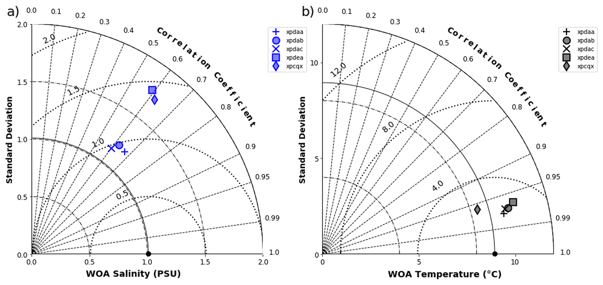
Figure 1 Taylor diagrams summarising the performance of the four control candidate simulations (XPDAA, XPDAB, XPDAC, XPDEA) in terms of their correlation, centred root-mean-square error, and ratio of variance to the NOAA World Ocean Atlas (a) salinity and (b) temperature databases (Zweng et al., 2019). The simulations were selected from a large FAMOUS pre-industrial perturbed parameter ensemble following the circulation performance screening described in Sect. 2.2. XPCQX represents the initial experiment, upon which the four control candidates aim to improve.

From this analysis, XPDAA returned the lowest root-mean-square error (RMSE) (and hence best performance using this metric; Fig. 1) for simulating both salinity (RMSE of 0.93 PSU) and temperature (RMSE of 2.21 ^∘C) and was thus used as our control simulation (Fig. 2). For comparison, HadCM3, the parent model of FAMOUS (Gordon et al., 2000), and the Model for Interdisciplinary Research on Climate 4m (MIROC4m) AOGCM (Sherriff-Tadano et al., 2021) have a RMSE of 1.06 PSU and 1.47 ^∘C and 0.59 PSU and 1.42 ^∘C, respectively.

Figure 2 (a) Salinity and (b) temperature profiles for the control simulation (centennial mean from final 100 years of a 5000-year simulation) along a transect crossing the Pacific–South Atlantic oceans.

The simulated steady-state AMOC strength in FAMOUS under fixed pre-industrial boundary conditions is approximately 17 Sv (Fig. 3a), which we consider to be in excellent agreement with direct modern AMOC observations from the RAPID AMOC array at 26.5^∘ N of 17.2 Sv from April 2004 to October 2012, and the depth of maximum meridional stream function at 26.5^∘ N is around 800 m (Fig. 3b), slightly shallower than RAPID observations of 900–1100 m (McCarthy et al., 2015; Sinha et al., 2018). In terms of the Atlantic circulation structure, the overturning cell of NADW descends to depths of 3000 m as it bridges into the South Atlantic, and AABW fills the bottom of the Atlantic basin with southern-sourced waters up to 20^∘ N. For the Nd isotope implementation, all sensitivity studies and model tuning described subsequently are based upon this simulation (XPDAA).

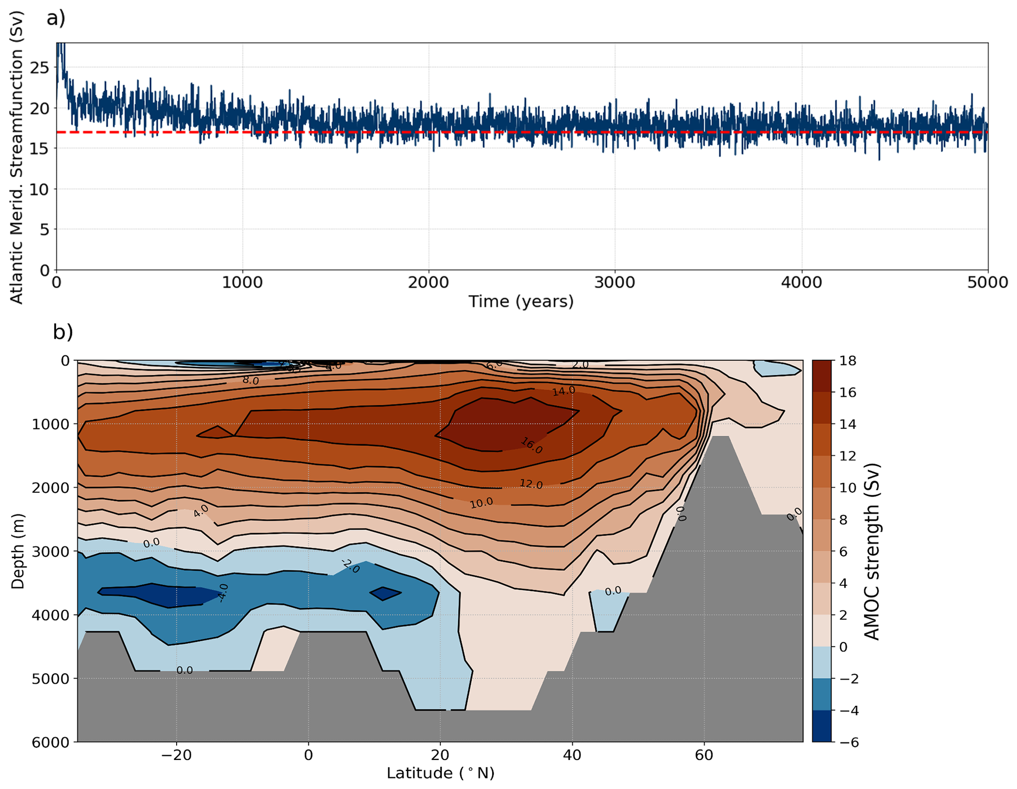
Figure 3 Atlantic meridional streamfunction for a 5000-year simulation using the control simulation (XPDAA), showing (a) the maximum streamfunction in time series (dashed red line indicates RAPID-AMOC 2004–2012 averaged AMOC strength at 26.5^∘ N of 17.2 Sv; McCarthy et al., 2015) and (b) the zonal integration calculated from the last 100 years.

2.3 Neodymium isotope implementation in FAMOUS

In our simulated Nd isotope scheme (Nd v1.0), we represent three different global sources of Nd into seawater: aeolian dust flux, dissolved riverine input, and seafloor sediment. Neodymium (Nd) here refers to the sum of ¹⁴³Nd and ¹⁴⁴Nd, and the isotopic ratio (IR) relates to the ratio of ¹⁴³Nd to ¹⁴⁴Nd, as shown in the following equations:

$$\begin{array}{}\text{(2)}& {\displaystyle }\mathrm{Nd}={}^{\mathrm{143}}\mathrm{Nd}+{}^{\mathrm{144}}\mathrm{Nd},\text{(3)}& {\displaystyle }\mathrm{IR}={\displaystyle \frac{{}^{\mathrm{143}}\mathrm{Nd}}{{}^{\mathrm{144}}\mathrm{Nd}}}.\end{array}$$

By rearranging Eq. (2) and using the isotopic ratio (IR: Eq. 3), individual fluxes of each isotope can be calculated (Eqs. 4 and 5) using information about Nd fluxes from each specific source and their associated IR distributions:

$$\begin{array}{}\text{(4)}& {\displaystyle }{}^{\mathrm{143}}\mathrm{Nd}={\displaystyle \frac{\mathrm{Nd}}{\left(\mathrm{1}+\left(\mathrm{1}/\mathrm{IR}\right)\right)}},\text{(5)}& {\displaystyle }{}^{\mathrm{144}}\mathrm{Nd}={\displaystyle \frac{\mathrm{Nd}}{\left(\mathrm{IR}+\mathrm{1}\right)}}.\end{array}$$

Neodymium isotopes are thus simulated and transported individually and independently as two separate tracers in our scheme, explicitly resolving the concentration and distribution of each Nd isotope, allowing for [Nd] and ε_Nd to be calculated offline from the model output.

The implementation of each source and sink term is described in detail in the following sections. To summarise these different components, Nd sources from aeolian dust fluxes and dissolved riverine input enter the ocean only via the uppermost near-surface ocean layer of the model. Seafloor sedimentary fluxes, an umbrella term that refers to a multitude of processes encompassing input from sediment deposited on the continental margins (Lacan and Jeandel, 2005), submarine groundwater discharge (Johannesson and Burdige, 2007), and an abyssal (i.e. below 3 km) benthic flux released from pore waters (Abbott et al., 2015a), are simulated via a combination of a sedimentary source applied across sediment–water interfaces together with a separate sink occurring via particle scavenging. Removal of Nd from the ocean model occurs when Nd scavenged or adsorbed onto sinking biogenic and lithogenic (dust) particles reaches the seafloor via vertical fluxes and undergoes sedimentation, acting as an active sink by removing the particle-associated Nd from the ocean.

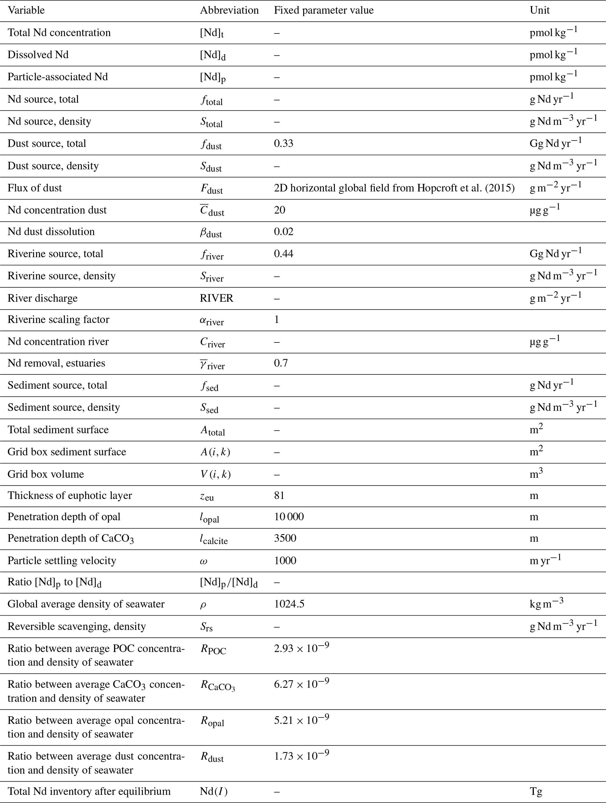
In the model numerics, fluxes of each Nd isotope into the ocean (kg m⁻³ s⁻¹) are multiplied by a factor of 10¹⁸. This technique is a common heuristic to assist human comprehension. It minimises the mathematical error associated with carrying small numbers (e.g. when manually checking the code inputs and outputs). Accordingly, concentrations of each Nd isotope in model units are in 10¹⁸ kg m⁻³. A full list of all variables described in the text and their abbreviations is given in Table 1.

Table 1 Nd scheme model parameters, abbreviations, fixed model parameter values, and units.

2.3.1 Dust source

Surface dust deposition (F_dust) is prescribed in the model from the annual mean dust deposition for the pre-industrial era as simulated by the atmosphere component of the Hadley Centre Global Environmental Model version 2 (HadGEM2-A) GCM (Collins et al., 2011) (Fig. 4a). The dust deposition scheme (described by Woodward, 2011) has been shown to be in generally good agreement with observations, with concentrations in the Atlantic simulated well across the whole of the Saharan dust plume; however, some discrepancies occur, including an overestimation at some Pacific sites during spring (Collins et al., 2011). The simulation of pre-industrial climate conditions within HadGEM2 are described by Hopcroft and Valdes (2015), and the dust results specifically are described in full by Hopcroft et al. (2015). Based on these simulated dust fluxes, we apply an Nd source per volume (S_dust: g m⁻³ yr⁻¹) in the uppermost layer of the ocean model, assuming a global mean concentration of Nd in dust ${\stackrel{\mathrm{‾}}{C}}_{\mathrm{dust}}$ (${\stackrel{\mathrm{‾}}{C}}_{\mathrm{dust}}=\mathrm{20}$ µg g⁻¹) (Goldstein et al., 1984; Grousset et al., 1988, 1998), from which only a certain fraction β_dust (β_dust=0.02: Greaves et al., 1994) dissolves in seawater.

$$\begin{array}{}\text{(6)}& S_{\mathrm{dust}}\left(i,k\right)={\displaystyle \frac{F_{\mathrm{dust}}\left(i,\mathrm{1}\right)\times {\stackrel{\mathrm{‾}}{C}}_{\mathrm{dust}}\times {\mathit{\beta }}_{\mathrm{dust}}}{\mathrm{d}z\left(i,\mathrm{1}\right)}}\end{array}$$

Here i,k represents the horizontal and vertical indexing of model grid cell and dz is the grid cell's thickness (10 m in the uppermost surface layer where k=1). The total global flux of Nd from surface aeolian dust deposition to seawater (f_dust) is 0.33 Gg yr⁻¹. Although we use an updated dust deposition field compared to previous studies, prescribed ${\stackrel{\mathrm{‾}}{C}}_{\mathrm{dust}}$ and β_dust are broadly consistent with earlier Nd isotope schemes, providing a comparable total Nd dust source (0.1–0.5 Gg yr⁻¹; Arsouze et al., 2009; Gu et al., 2019; Pöppelmeier et al., 2020b; Rempfer et al., 2011; Tachikawa et al., 2003).

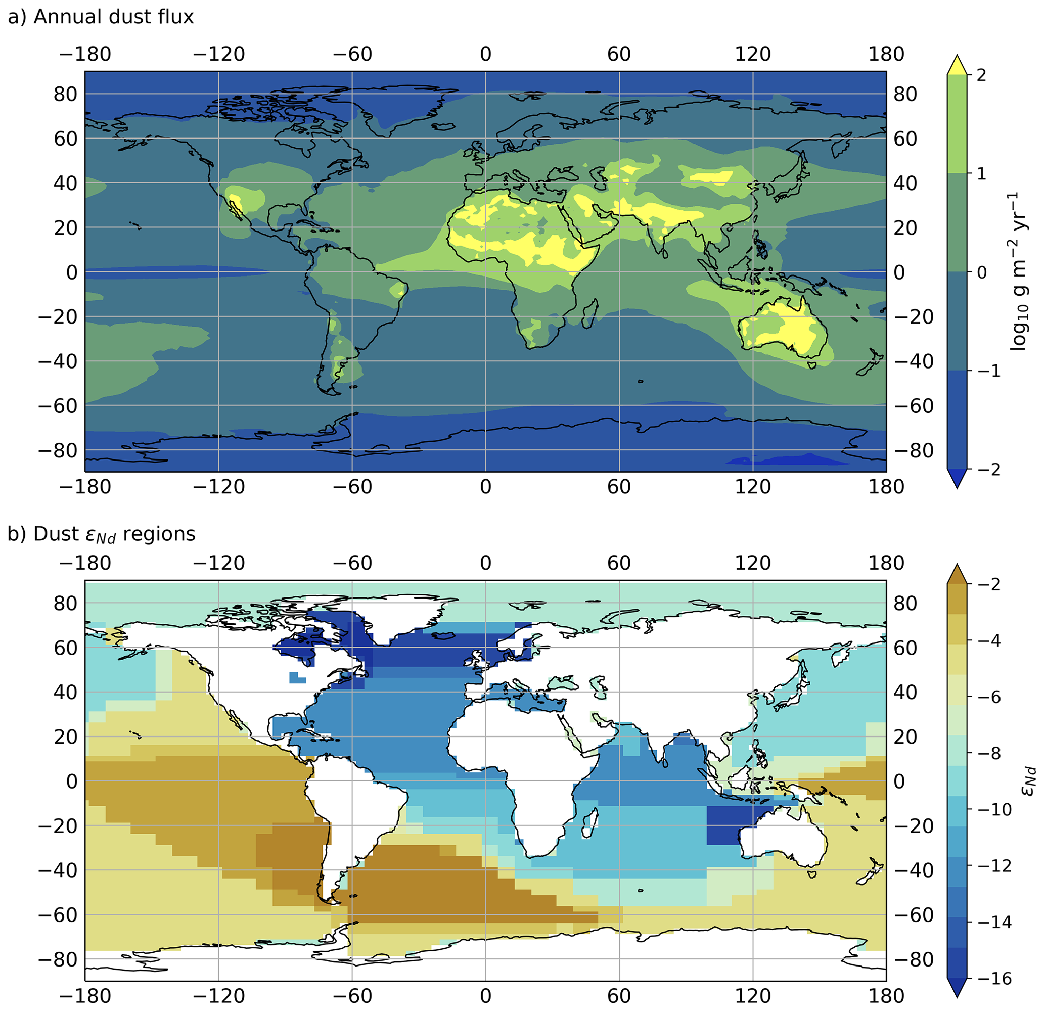
Figure 4 (a) Annual dust deposition taken from the pre-industrial annual mean dust deposition simulated by HadGEM2-A GCM (Hopcroft et al., 2015). (b) The ε_Nd signal from dust deposition following Tachikawa et al. (2003) and updated with information from Mahowald et al. (2006) and Blanchet (2019).

For the Nd isotope compositions of the dust flux, we started with the first-order estimate by Tachikawa et al. (2003), as follows: North Atlantic >50^∘ N: ${\mathit{\epsilon }}_{\mathrm{Nd}}=-\mathrm{15}$; Atlantic <50^∘ N: ${\mathit{\epsilon }}_{\mathrm{Nd}}=-\mathrm{12}$; North Pacific >44^∘ N: ${\mathit{\epsilon }}_{\mathrm{Nd}}=-\mathrm{5}$; Indo-Pacific <44^∘ N: ${\mathit{\epsilon }}_{\mathrm{Nd}}=-\mathrm{7}$; and remainder:
${\mathit{\epsilon }}_{\mathrm{Nd}}=-\mathrm{8}$. This was revised with additional constraints, accounting for the dust plume expansions as reported by Mahowald et al. (2006), in combination with detrital Nd isotope data by Blanchet (2019) (Fig. 4b). For this, the mean detrital isotopic signature of a source region (e.g. the Sahara) was calculated and then applied to the region where this dust is deposited over the ocean based on the plume expansion by Mahowald et al. (2006) (for the example of the Sahara this is the North Atlantic). Regions in between major dust plumes were linearly interpolated. For the polar regions no constraints are available, and a default value has been assigned instead, but the lack of dust deposition in these regions ensures that this has no impact on the Nd cycle.

2.3.2 Dissolved riverine source

To represent the Nd source from dissolved river fluxes, we used the river outflow to the ocean simulated by FAMOUS (RIVER) as our river water discharge (g m⁻² yr⁻¹) and combined this outflow with both the Nd concentration (C_river; µg g⁻¹) and isotopic concentration (used to calculate the flux from each Nd isotope using Eqs. 4 and 5) of river water dissolved material, as estimated by Goldstein and Jacobsen (1987; see Table 3). All river source Nd fields are shown in Fig. 5.

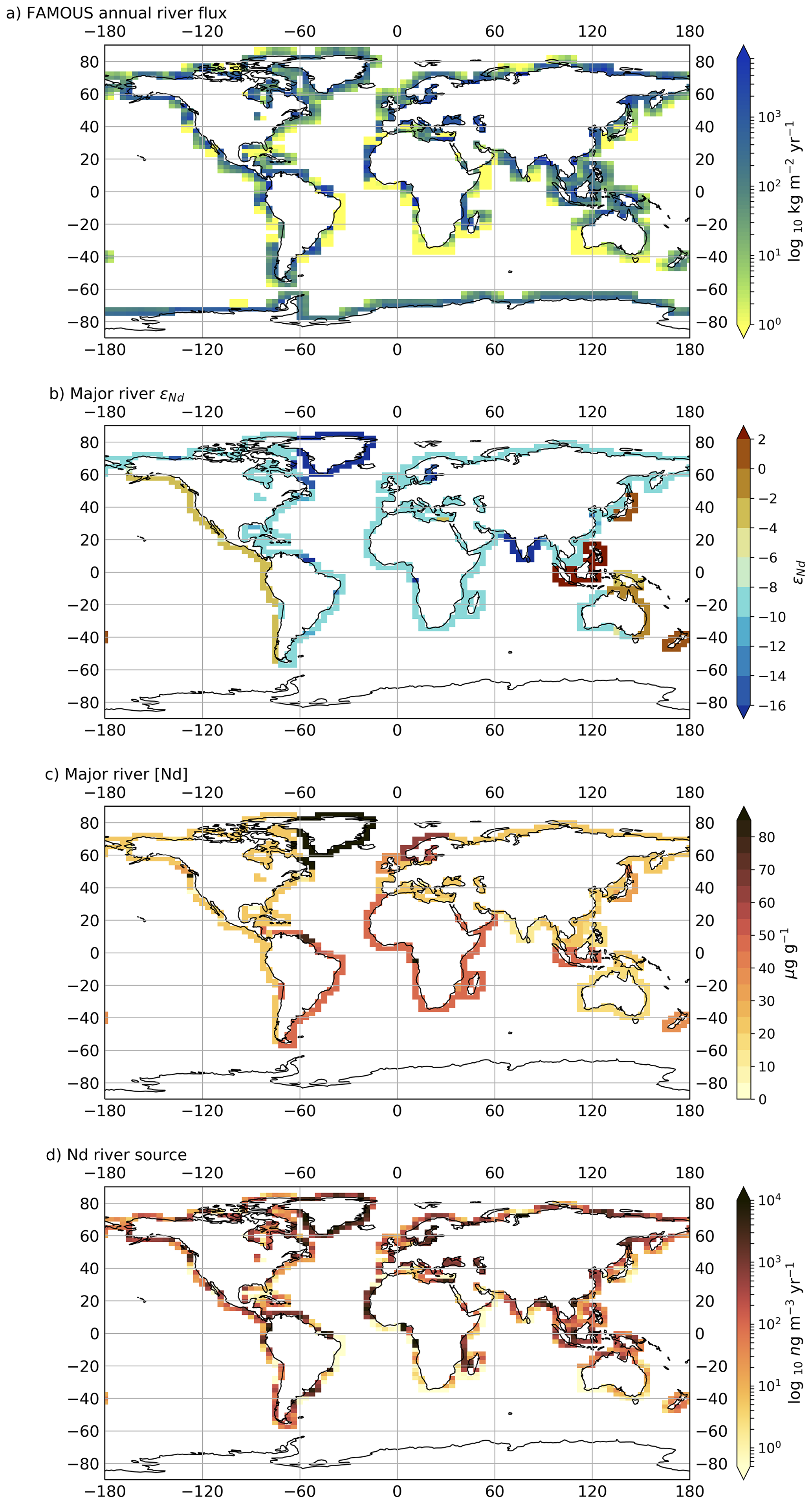
Figure 5 (a) Simulated river outflow (RIVER) in FAMOUS, (b) major river ε_Nd, (c) major river [Nd], and (d) the resulting riverine Nd source. The coastal grids in (b) and (c) are prescribed following average [Nd] and ε_Nd estimates of dissolved river runoff to each of the oceans by Goldstein and Jacobsen (1987; see Table 3).

River outflow in FAMOUS is based on a routing scheme that instantaneously delivers terrestrial runoff (precipitation − [evaporation + soil moisture]) from the location that precipitation falls to the designated coastal grid cell that the runoff would reach due to river routing (i.e. the river mouth). Relating the riverine Nd flux to the model's prognostic river discharge allows the Nd river source to respond to different climatic conditions, making it a more dynamic and predictive tool for examining the impact of changes in the global hydrological balance, such as wetting and drying events or shifts in the monsoons. Essentially, river outflow plumes are “tagged” with the estimated ε_Nd (which is provided as an input map along the coasts; Fig. 5b) according to the model's projected water discharge at that location and C_river (also provided as an input map along the coasts; Fig. 5c). For palaeoclimate or future climate applications where river routing is significantly different from today, the input maps controlling C_river tagging at the coast would need to be updated to reflect Nd dissolution from the modified fluvial pathway over land (the model should predict the rest).

Estuaries are important biogeochemical reactors of rare-earth elements (REEs), with sea salt driving flocculation of river-dissolved organic matter, which results in estuarine REE removal (Elderfield et al., 1990). This removal is known to be important in balancing the marine REE budgets; however, the complex processes involved are still not fully constrained (Elderfield et al., 1990). Rousseau et al. (2015) summarised published observations of Nd removal (%) in estuaries from observations of estuarine dissolved Nd dynamics (Rousseau et al., 2015; their Table 1). Published values (n=17) range from 40 % in Tamar neaps (Elderfield et al., 1990) to 97 % in the Amazon (Sholkovitz, 1993), with a mean Nd removal of 71 ± 16 % SD. Based upon this, and parallel to previous model schemes (e.g. Rempfer et al., 2011; Gu et al., 2019; Arsouze et al., 2009), we assume that 70 % of dissolved Nd from river systems are removed in estuaries (i.e. ${\stackrel{\mathrm{‾}}{\mathit{\gamma }}}_{\mathrm{river}}=\mathrm{0.7}$).

The dissolved riverine source per unit volume of Nd (S_river: g m⁻³ yr⁻¹) in the uppermost layer of the ocean is therefore calculated as follows:

$$\begin{array}{}\text{(7)}& S_{\mathrm{river}}\left(i,k\right)={\displaystyle \frac{\mathrm{RIVER}\left(i,\mathrm{1}\right)\times C_{\mathrm{river}}\times \left(\mathrm{1.0}-{\stackrel{\mathrm{‾}}{\mathit{\gamma }}}_{\mathrm{river}}\right)}{\mathrm{d}z\left(i,\mathrm{1}\right)}}.\end{array}$$

The total global flux of river-sourced dissolved Nd to seawater in the model (f_river) is 0.44 Gg yr⁻¹. Previous Nd isotope schemes have applied either fixed annual mean continental river discharge estimates from Goldstein and Jacobsen (1987) and Dai and Trenberth (2002), as applied in the Bern3D Nd isotope scheme (Rempfer et al., 2011; Pöppelmeier et al., 2021a), or, similar to this study, using the model's own river routing and discharge schemes, as with NEMO-OPA (Arsouze et al., 2009) and CESM1 (Gu et al., 2019). Our estimated global total dissolved riverine Nd source to the oceans sits within previous model estimates (0.26–1.7 Gg yr⁻¹; Arsouze et al., 2009; Gu et al., 2019; Pöppelmeier et al., 2020b; Rempfer et al., 2011; Tachikawa et al., 2003).

There is a larger range in estimated riverine Nd flux to the ocean relative to the estimated dust flux ranges. It should be noted that the largest simulated Nd river source amongst these studies (1.7 Gg yr⁻¹; Pöppelmeier et al., 2020b) in the updated Bern3D Nd isotope scheme applied a river scaling factor, used as a tuning parameter and based on findings by Rousseau et al. (2015), who suggest a globally significant release of Nd to seawater by dissolution of river-sourced lithogenic suspended sediments grounded upon observations in the Amazon estuary. Our model does not attempt to fully resolve all complex estuarine processes, and in this study we chose to represent the dissolved riverine flux as a single source to seawater. Furthermore, our sediment Nd source to the ocean (described Sect. 2.3.3), which occurs across sediment–water interfaces, utilises the continental margin and seafloor ε_Nd distribution maps by Robinson et al. (2021), thus using the most recent compilation of published global observations of Nd isotope compositions of river sediment samples deposited on the continental shelf and slopes (alongside geological outcrops and marine sediment samples). It is therefore likely that this margin source encompasses (at least in part) the Nd isotope fingerprint from a river particle flux.

2.3.3 Continental margin and seafloor sediment source

The sediment source describes the flux of Nd into seawater entering each model grid cell adjacent to sediment. This source is not restricted to the uppermost surface layers and can be implemented across all vertical and horizonal sediment–water interfaces, as is the case for all experiments described in this study. As such, the sediment source represents (1) input from sediment deposited on the continental margins (Lacan and Jeandel, 2005), (2) submarine groundwater discharge, as suggested by Johannesson and Burdige (2007), which releases Nd to seawater via discharge of fresh groundwater to coastal seas and is mainly limited to the upper 200 m, and (3) a benthic flux, which specifically refers to a transfer of Nd from sediment pore water to seawater resulting from early diagenetic reactions and is not depth limited (Abbott et al., 2015b, a; Haley et al., 2017).

The total sediment Nd source per unit volume (S_sed: g m⁻³ yr⁻¹) into any given ocean grid cell is dependent on the fraction of the surface area of that cell that is in contact with sediment. Similar to previous schemes (e.g. Gu et al., 2019; Pöppelmeier et al., 2020b; Rempfer et al., 2011), the total globally integrated sediment-associated Nd source to the ocean (f_sed: g Nd yr⁻¹) is used as a tuning parameter.

$$\begin{array}{}\text{(8)}& S_{\mathrm{sed}}\left(i,k\right)=f_{\mathrm{sed}}\times {\displaystyle \frac{A\left(i,k\right)}{A_{\mathrm{total}}}}\times {\displaystyle \frac{\mathrm{1}}{V\left(i,k\right)}},\end{array}$$

where A(i,k) is the total area of the sediment surface in contact with seawater per ocean grid cell (m²), A_total is the total global area of the sediment surface where a sediment source occurs (m²), and V(i,k) is the volume of water per ocean grid cell (m³).

There is still no true consensus on whether (and how) to apply spatial variability to sediment Nd sources, as reflected in the way previous schemes have adopted different approaches. Arsouze et al. (2009) limited the sediment flux to the upper 3000 m of the ocean, imposing a depth-scaling factor and considering estimated [Nd] distributions across the continental margins. Both Rempfer et al. (2011) and Gu et al. (2019) simplified this method by applying spatially uniform sediment Nd fluxes, also limited to the upper 3000 m. In more recent work, Pöppelmeier et al. (2020b) removed the depth limitation (as we have done), and incorporated a geographically varying scaling factor to try to capture more localised features through increased benthic fluxes (Abbott et al., 2015b; Blaser et al., 2020; Grenier et al., 2013; Lacan and Jeandel, 2005; Rahlf et al., 2020). Pasquier et al. (2022) presented the first inverse model of global marine cycling of Nd, and the strength of the sediment Nd flux to the ocean was imposed with an exponential depth function, resembling eddy kinetic energy and particulate organic matter fluxes, which are characteristically larger near the surface and in coastal regions.

For our scheme, we do not assume spatial variations in the sediment source of Nd (f_sed), essentially avoiding making explicit inferences on the nature of the sedimentary Nd source. It has been proposed that preferential mobilisation of certain components of the sediment drive spatial variations in sediment fluxes (e.g. Abbott et al., 2015a; Wilson et al., 2013; Du et al., 2016; Abbott, 2019; Abbott et al., 2019) and that both detrital and authigenic phases likely exchange Nd within pore water during early diagenesis (Du et al., 2016; Blaser et al., 2019b). However, the elusiveness of marine Nd cycling alongside our limited knowledge of the specific mechanisms controlling sediment–water Nd interactions mean that determining generalisable rules for where and under what conditions (e.g. redox environments or fresh labile detrital material) preferential mobilisation may occur is unknown and challenging to resolve. Therefore, in accordance with Pöppelmeier et al. (2020a), Du et al. (2020), Gu et al. (2019), and Rempfer et al. (2011), we adopt a constant detrital sediment flux as a first-order approximation. In fact, we contend that applying this simpler method, as opposed to constructing a more complex source term that is arguably just as arbitrary (given the uncertainty in Nd cycling), allows for a more explicit quantification of differences between observed and simulated Nd distributions. As such, without overfitting our model, we allow for the clearest indication of those parts of the system that are well understood (and represented) and those which prove deficient. Under this framework, we may separate out and test the effect of many of the major Nd sources and sinks with dedicated sensitivity simulations, including the possibility in future work of incrementally modifying the sediment source distributions to increase the complexity of the scheme and assess the impact of our various assumptions.

The isotopic ratio of the sediment Nd flux to seawater is prescribed using the recently updated global gridded map of bulk detrital ε_Nd at the continental margins and seafloor (Robinson et al., 2021, Fig. 6a). Using Eqs. (4) and (5), fluxes of each Nd isotope are calculated from this condition and bi-linearly regridded to the model's native resolution (Fig. 6b).

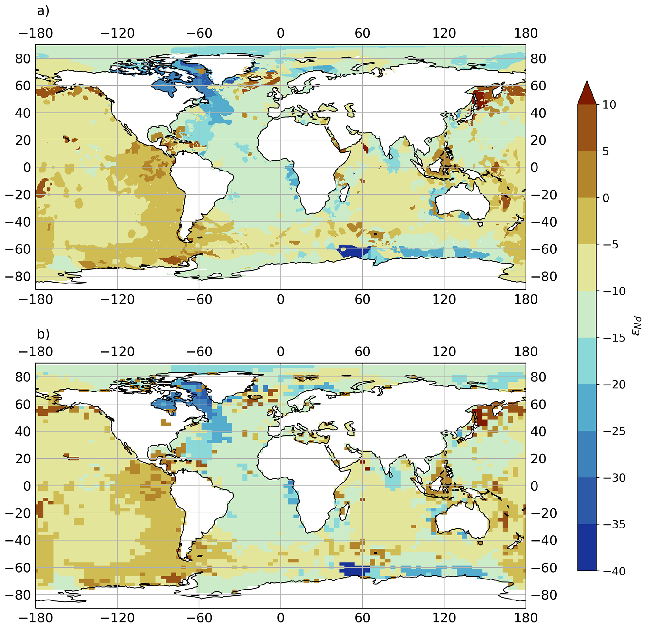
Figure 6 (a) Map of the global ε_Nd distributions at the sediment–ocean interface from Robinson et al. (2021) and (b) as used as a model input in this study (bi-linearly regridded from (a) onto the coarser FAMOUS ocean grid).

Pasquier et al. (2022) first applied the sedimentary ε_Nd map from Robinson et al. (2021) in their recent global marine Nd isotope scheme, imposing positive (i.e. radiogenic) modifications to the Pacific sedimentary ε_Nd and using a reactivity scaling factor (linked to sediment lability) that favours more extreme ε_Nd signals. Here, we again adopt a simpler approach, imposing the unmodified sediment ε_Nd distributions from Robinson at al. (2021), allowing for a presentation of our new scheme based on what we confidently know about Nd cycling without the complication of over-conditioning our model inputs. Future research may then use this work as a foundation to robustly explore different choices for model inputs (i.e. boundary conditions) to revisit these fundamental questions about Nd sediment source.

2.3.4 Internal cycling via reversible scavenging

Vertical cycling and removal of Nd from the water column via sinking particles (“reversible scavenging”) is parameterised using the same approach as previous Nd isotope implementations (Siddall et al., 2008; Arsouze et al., 2009; Rempfer et al., 2011; Gu et al., 2019; Pöppelmeier et al., 2020a; Oka et al., 2021). Based on the original scheme of Bacon and Anderson (1982), the method captures the physical process of absorption or incorporation and desorption or dissolution of Nd onto particle surfaces in seawater. The scheme assumes that particle-associated Nd is in dynamic equilibrium with falling particles throughout the water column, with continuous exchange between the particle and dissolved pools. This process redistributes Nd within the water column, acting as a net sink of dissolved Nd at shallower depths as they adsorb onto particle surfaces and a net source at greater depths where dissolution of particles releases dissolved Nd back to seawater. The scavenging is the only sink of Nd in our model; Nd associated with particles (particulate organic carbon, POC; calcium carbonate, CaCO₃; opal; dust) reaching the seafloor is removed from the system, operating under a steady-state assumption that acts to balance the three external input sources (marine sediments, dust, and rivers). Previous studies (e.g. Siddall et al., 2008; Arsouze et al., 2009; Rempfer et al., 2011; Gu et al., 2019; Wang et al., 2021) have demonstrated that reversible scavenging is an active and important component in global marine Nd cycling and is necessary for successfully simulating both [Nd]_d and ε_Nd distributions.

Updating the approach employed by Siddall et al. (2008), we prescribed individual biogenic particle export fields based on satellite-derived primary production. FAMOUS does contain an optional ocean biogeochemistry module (Hadley Centre Ocean Carbon Cycle; HadOCC), which includes simplified nutrient, phytoplankton, zooplankton, and detritus (NPZD) classes (Palmer and Totterdell, 2001) and could instead be used as the basis for predicting vertical particle fluxes in the ocean (which was the approach adopted by Arsouze et al., 2009; Gu et al., 2019; and Rempfer et al., 2011). We favoured satellite-derived estimates in order to improve the accuracy of particle-associated cycling of Nd and reduce biases inherent to the intermediate-complexity biogeochemistry model (Dentith et al., 2020; Palmer and Totterdell, 2001). This approach also optimises the computational efficiency of our scheme.

In our scheme, biogenic particle fields (POC, CaCO₃, and opal) are prescribed using gridded, global satellite-derived particle export productivity from Dunne et al. (2012, 2007). The euphotic zone (z_eu) is set to a globally uniform depth in FAMOUS of 81 m, which is the closest bottom grid box depth to match that defined in the OCMIP II protocol (75 m) (Najjar and Orr, 1998). Below z_eu, appropriate depth-dependent dissolution profiles, derived from assumptions of particle degradability and sinking speed (Martin et al., 1987; Laws et al., 2000; Behrenfeld and Falkowski, 1997) and widely used to model flux attenuation in ocean models (e.g. all models used in the Ocean Carbon-Cycle Model Intercomparison Project; Doney et al., 2004; Sarmiento and Le Quéré, 1996), were applied to the biogenic export fluxes.

Downward fluxes of POC (F_POC) follow the power law profile of Martin et al. (1987):

$$\begin{array}{}\text{(9)}& F_{\mathrm{POC}}\left(z\right)=F_{\mathrm{POC}}\left(z_{\mathrm{eu}}\right)\times {\left({\displaystyle \frac{z}{z_{\mathrm{eu}}}}\right)}^{-\propto }\left(\text{for}z>z_{\mathrm{eu}}\right),\end{array}$$

where z is depth (m) and ∝ represents a dimensionless dissolution constant for POC set to 0.9 (Najjar and Orr, 1998). Although a widely used parameterisation of dissolution, it should be noted this so-called “Martin curve” is known to underestimate the flux to the sediment in the off-equatorial tropics and subtropics and overestimates the flux in subpolar regions, indicating particles penetrate deeper than the Martin curve in the tropics and shallower in sub-polar regions (Dunne et al., 2007).

Downward fluxes of opal (F_opal) and CaCO₃ ($F_{{\mathrm{CaCO}}_{\mathrm{3}}}$) follow exponential dissolution profiles with particle-specific length scales, i.e. l_opal (10 000 m) and l_calcite (3500 m) (Maier-Reimer, 1993; Henderson et al., 1999; Najjar and Orr, 1998), respectively, calculated as follows:

$$\begin{array}{}\text{(10)}& {\displaystyle }{F}_{\mathrm{opal}}\left(z\right)=F_{\mathrm{opal}}\left(z_{\mathrm{eu}}\right)\times \exp \left({\displaystyle \frac{z_{\mathrm{eu}}-z}{l_{\mathrm{opal}}}}\right),\text{(11)}& {\displaystyle }{F}_{{\mathrm{CaCO}}_{\mathrm{3}}}\left(z\right)=F_{{\mathrm{CaCO}}_{\mathrm{3}}}\left(z_{\mathrm{eu}}\right)\times \exp \left({\displaystyle \frac{z_{\mathrm{eu}}-z}{l_{{\mathrm{CaCO}}_{\mathrm{3}}}}}\right).\end{array}$$

The sinking of dust is prescribed according to the pre-industrial annual mean dust deposition simulated by Hopcroft et al. (2015) (see Sect. 2.3.1). We assume that dust does not dissolve significantly with depth, and thus dust export fluxes are constant throughout the water column. In line with previous schemes (e.g. Arsouze et al., 2009; Pöppelmeier et al., 2020b; Rempfer et al., 2011; Siddall et al., 2008), a uniform settling velocity (ω) of 1000 m yr⁻¹ is applied to all particle fields. Although we acknowledge this is a simplification, the uniform settling rate applied captures the mean particle flux to the seafloor.

Annual averaged export of biogenic fields is shown in Fig. 7, and the total annual export production of POC (9.6 Gt(C) yr⁻¹), CaCO₃ (0.45 Gt(C) yr⁻¹), and opal (90 Tmol(Si) yr⁻¹) are comparable with previous estimates, although export of CaCO₃ and opal are at the lower end, as highlighted in Table 3 by Dunne et al. (2007). Note that the annual export of CaCO₃ reflects the new optimised surface calcite parameterisation as described in Dunne et al. (2012).

Figure 7 Particle export fields from the ocean surface (g m⁻² yr⁻¹). Biogenic particle fields are prescribed using satellite-derived export productivity fields for (a) POC, (b) CaCO₃, and (c) opal (Dunne et al., 2007, 2012). The dust input fields (d) are annual mean dust deposition simulated for the pre-industrial era by the HadGEM2-A GCM (Hopcroft et al., 2015). Note the different scale used for panel (a).

Reversible scavenging (Nd_rs) considers total Nd for each isotope (j) as the dissolved Nd (Nd_d) and particulate Nd (Nd_p) associated with the different particle fields (χ, where χ refers to POC, CaCO₃, opal, and dust).

$$\begin{array}{}\text{(12)}& {\left[\mathrm{Nd}\right]}_{\mathrm{t}}^j={\left[\mathrm{Nd}\right]}_{\mathrm{d}}^j+{\left[\mathrm{Nd}\right]}_{\mathrm{p}}^j={\left[\mathrm{Nd}\right]}_{\mathrm{d}}^j+{\sum }_{\mathit{\chi }}{\left[\mathrm{Nd}\right]}_{\mathrm{p},\mathit{\chi }}^j\end{array}$$

Nd_p sinks in the water-column with the particles due to gravitational force. Dissolution of biogenic particles with increasing depth below the euphotic zone releases Nd incorporated or adsorbed onto particles back to seawater (i.e. the Nd is dissolved or desorbed). Thus, particles act as internal sinks for marine Nd_d in shallower depths and as sources at greater depths. This combined process for reversible scavenging (S_rs) in the model can be described by

$$\begin{array}{}\text{(13)}& S_{\mathrm{rs}}\left(i,k\right)={\displaystyle \frac{-\partial \left(\mathit{\omega }{\left[\mathrm{Nd}\right]}_{\mathrm{p}}\left(i,k\right)\right)}{\partial z\left(i,k\right)}},\end{array}$$

where [Nd]_p can be determined within the model from total Nd for each isotope as follows:

$$\begin{array}{}\text{(14)}& {\left[\mathrm{Nd}\right]}_{\mathrm{p}}^j\left(i,k\right)={\left[\mathrm{Nd}\right]}_{\mathrm{t}}^j\left(i,k\right)\times \left(\mathrm{1}-{\displaystyle \frac{\mathrm{1}}{\mathrm{1}+{\sum }_{\mathit{\chi }}{R}_{\mathit{\chi }}\left(i,k\right)\times K_{\mathit{\chi }}^j}}\right).\end{array}$$

Rχ(i,k) describes the dimensionless ratio between particle concentration for each particle type (Cχ(i,k)) and the average density of seawater (ρ: 1024.5 kg m⁻³), input as fixed boundary conditions in our scheme. Cχ is calculated from the prescribed particle fluxes (Fχ: Fig. 7) by assuming a globally uniform settling velocity (ω=1000 m yr⁻¹; Arsouze et al., 2009; Dutay et al., 2009; Gu et al., 2019; Kriest and Oschlies, 2008; Rempfer et al., 2011), i.e. $C\mathit{\chi }=F\mathit{\chi }/\mathit{\omega }$. The equilibrium between dissolved concentration ([Nd]_d) and concentration associated with particle type ([Nd]_p) can be described by the equilibrium partition coefficient ($K_{\mathit{\chi }}^j$):

$$\begin{array}{}\text{(15)}& K_{\mathit{\chi }}^j={\displaystyle \frac{{\left[\mathrm{Nd}\right]}_{\mathrm{p},\mathit{\chi }}^j}{{\left[\mathrm{Nd}\right]}_{\mathrm{d}}^j}}\times {\displaystyle \frac{\mathrm{1}}{{\stackrel{\mathrm{‾}}{R}}_{\mathit{\chi }}}},\end{array}$$

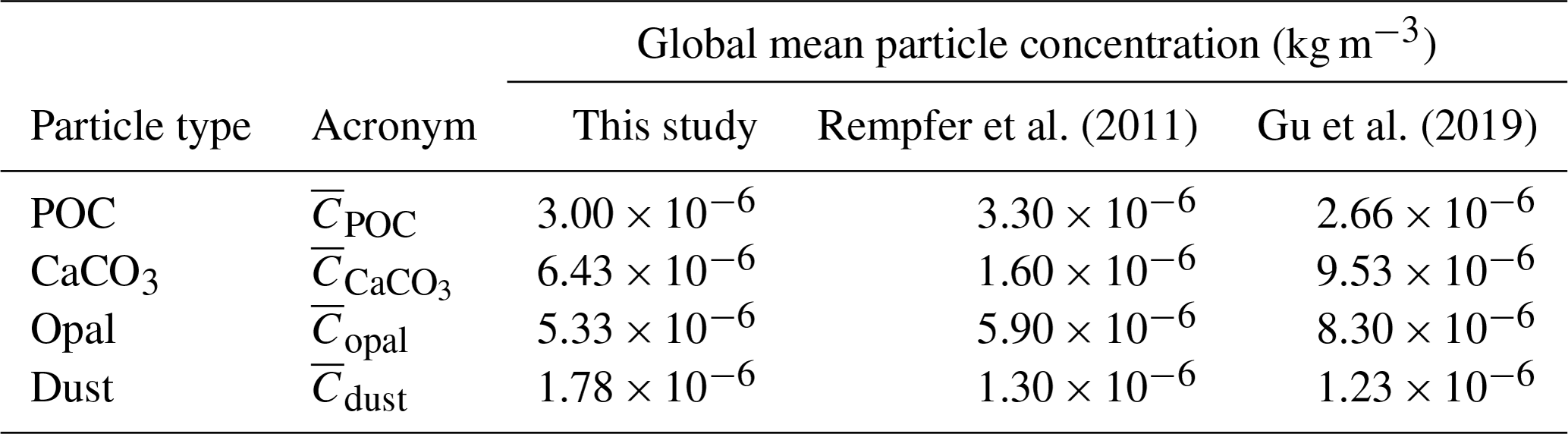
where $[\mathrm{Nd}{]}_{\mathrm{p}}/[\mathrm{Nd}{]}_{\mathrm{d}}$ represents the scavenging efficiency in the model. It is independent of particle type and is used as a tuning parameter. ${\stackrel{\mathrm{‾}}{R}}_{\mathit{\chi }}$, however, is dependent on particle type (where ${\stackrel{\mathrm{‾}}{R}}_{\mathit{\chi }}={\stackrel{\mathrm{‾}}{C}}_{\mathit{\chi }}/\mathit{\rho }$), and thus Kχ is different for different particles. Our global mean particle concentrations (${\stackrel{\mathrm{‾}}{C}}_{\mathit{\chi }}$; Table 2) are similar to those reported in previous schemes.

Table 2 Global mean particle concentrations for each particle type used to calculate equilibrium scavenging coefficients following Eq. (15). In summary, export fluxes of POC, CaCO₃, and opal in this study are from Dunne et al. (2007, 2012), while dust fluxes are from Hopcroft et al. (2015). Global mean particle concentrations reported in previous Nd isotope schemes are shown for comparison.

Isotopic fractionation during absorption or incorporation and desorption or dissolution is neglected due to similar masses of ¹⁴³Nd and ¹⁴⁴Nd, avoiding undue complexity arising from any assumption about preferential scavenging (Siddall et al., 2008). Adsorption occurs everywhere that particles are present and we do not allow for preferential scavenging onto different particle types, consistent with previous models (e.g. Rempfer et al., 2011).

Therefore, by including advection and diffusion processes (transport), the total conservation equation for each Nd isotope in the model scheme can be written as follows:

$$\begin{array}{}\text{(16)}& {\displaystyle \frac{\mathit{\delta }{\left[\mathrm{Nd}\right]}_{\mathrm{t}}^j}{\mathit{\delta }t}}=S_{\mathrm{dust}}^j+S_{\mathrm{river}}^j+S_{\mathrm{sed}}^j+S_{\mathrm{rs}}^j+\mathrm{transport}.\end{array}$$

2.4 Evaluation methods and data sets

To validate the new Nd isotope scheme (Nd v1.0) and to assess the model's performance, we compare the simulated [Nd]_d and ε_Nd to modern seawater measurements, with a focus on describing the ability of the model to represent key spatial and vertical distributions across ocean basins.

As part of this assessment, a basic indication of model skill is returned by the mean absolute error (MAE):

$$\begin{array}{}\text{(17)}& \mathrm{MAE}={\displaystyle \frac{\mathrm{1}}{N}}{\sum }_{k=\mathrm{1}}^N\left|{\mathrm{obs}}_k-{\mathrm{sim}}_k\right|,\end{array}$$

where obs_k and sim_k are measured and simulated [Nd]_d or ε_Nd, respectively, N is the number of observations, and k is an index over all observational data. For each measurement – based on its longitude, latitude, and depth – the value predicted by the model is extracted and the mean deviation of simulated and observed [Nd]_d and ε_Nd is presented (in pmol kg⁻¹ and epsilon units, respectively). Here we chose specifically not to apply a grid box volume weighting to the MAE, which would act to emphasise abyssal Pacific results in our assessment of model skill, where there are few observations and relatively low variability in Nd distributions. The advantage of using an unweighted MAE is that the assessment metric better scrutinises regions with larger (spatial) gradients in both [Nd]_d or ε_Nd, i.e. at the surface and high latitudes. We also report root-mean-square error (RMSE) for each simulation as an additional indicator of model skill and to allow for additional comparability with other studies:

$$\begin{array}{}\text{(18)}& \mathrm{RMSE}=\sqrt{{\displaystyle \frac{\mathrm{1}}{N}}{\sum }_{k=\mathrm{1}}^N{\displaystyle \frac{({\mathrm{obs}}_k-{\mathrm{sim}}_k{)}^{\mathrm{2}}}{N}}}.\end{array}$$

The observational data used in this assessment are from the seawater REE compilation used by Osborne et al. (2017, 2015), augmented with more recent measurements including data in the GEOTRACES Intermediate Data Product 2021 (GEOTRACES Intermediate Data Product Group, 2021) from GEOTRACES cruises (GA02, GA08, GP12, GN02, GN03 and GIPY05). Combined, our observational database represents a total of 6048 [Nd]_d and 3278 ε_Nd measurements, making it the largest compilation of seawater Nd data used to date to validate the performance of an Nd-isotope-enabled model. Notably, we omit measurements of [Nd]_d>100 pmol kg⁻¹ from the model data comparison because they represent very localised signals that we do not attempt to resolve. These include extreme surface concentrations present in restricted basins, such as fjords, the Baltic Sea, and the Gulf of Alaska (Chen et al., 2013; Haley et al., 2014), or input from hydrothermal activity (Chavagnac et al., 2018), which is not believed to govern global marine Nd distributions due to the immediate removal of hydrothermal Nd at the vent site (Goldstein and O'Nions, 1981). The location and spatial distribution of all observational records used in this study are shown in Fig. 8, and full details of the seawater compilation including a full list of all the references for the data sources are provided in Table S3 in the Supplement.

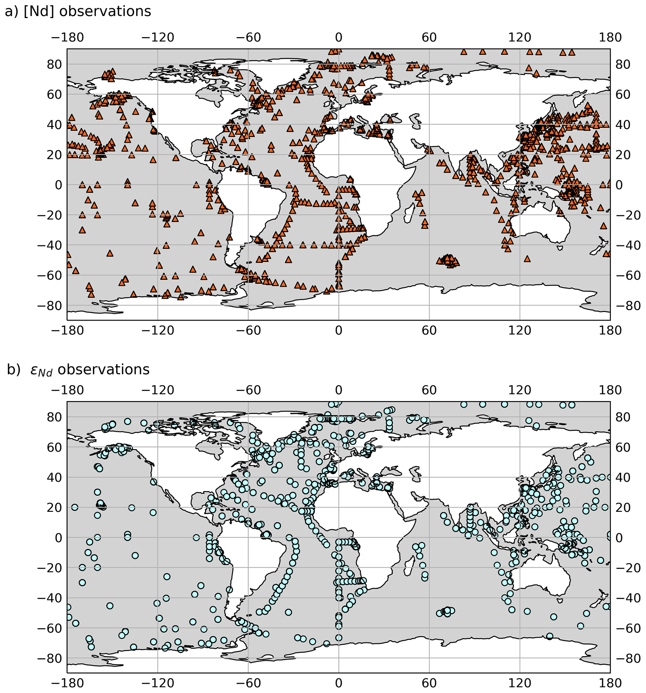
Figure 8 Location of marine observational records used in this study: (a) filled orange triangles show the location of dissolved Nd concentration records, while (b) filled sky-blue circles show the location of dissolved ε_Nd records.

Neither the horizontal nor vertical distribution of global seawater [Nd]_d and ε_Nd observational data is even. Most [Nd]_dmeasurements are in the Pacific Ocean. This is in contrast to ε_Nd measurements, which are most frequent in the Atlantic Ocean. Both [Nd]_d and ε_Nd observational data are biased towards shallower depths. It is therefore important to highlight that (as with previous studies) a skew in the distribution of seawater Nd measurements will act to bias our assessment of model performance.

In some instances, the location of the compared measured and modelled Nd may not match due to the coarseness of the model grid near land grid cells. In such cases, we employ a nearest neighbour algorithm to extract the modelled value from the closest ocean model grid cell. Furthermore, if multiple measurements occur within one model grid cell, the arithmetic mean of the values is used for our comparison to model results, and as such n is 3471 and 2136 for the calculation of MAE_[Nd] and MAE_εNd, respectively.

To ensure that our evaluation is not overly reliant on the cost function analysis alone, and hence evaluated the spatial biases in our assessment from the geographically uneven spread of measured [Nd]_d and ε_Nd, we also assess the capability of the model to reproduce appropriate global Nd inventories and to simulate large-scale horizontal and vertical gradients. We compare our results briefly with findings from previous modelling studies, but we highlight that the purpose of this study is to understand the behaviour of our model and not to undertake a comprehensive calibration of its performance. Optimisation (or “tuning”) of the Nd scheme will follow this work, and this needs to be considered when comparing the cost function performance to previous schemes.

2.5 Sensitivity experiment design

We designed a number of sensitivity experiments (Table 3) to systematically vary individual model parameters describing the reversible scavenging efficiency ($[\mathrm{Nd}{]}_{\mathrm{p}}/[\mathrm{Nd}{]}_{\mathrm{d}}$) and the main Nd source (f_sed). These two parameters ($[\mathrm{Nd}{]}_{\mathrm{p}}/[\mathrm{Nd}{]}_{\mathrm{d}}$ and f_sed) were chosen primarily as they represent important and largely unconstrained non-conservative processes that are understood to govern simulated global distributions of both seawater [Nd]_d and ε_Nd (Rempfer et al., 2011; Pöppelmeier et al., 2020a; Gu et al., 2019; Arsouze et al., 2009; Siddall et al., 2008). By isolating individual effects, the primary aim was to attain a detailed understanding of the model's sensitivity to different forcings, to identify which parameters are important for [Nd]_d and/or ε_Nd patterns, and to identify assumptions within the explored parameters that require further constraining (through further field campaigns, laboratory analyses, or model experimentation).

Table 3 Suite of FAMOUS simulations designed to assess the sensitivity of simulated [Nd]_d and ε_Nd distributions to two systematically varied parameters: reversible scavenging efficiency ($[\mathrm{Nd}{]}_{\mathrm{p}}/[\mathrm{Nd}{]}_{\mathrm{d}}$) and the global rate of direct Nd transfer from sediment to ocean water (f_sed). Simulation name refers to the title given to each sensitivity simulation in this paper, and the simulation identifier refers to the unique five-letter Met Office identifier (which, for example, can be used to call down full experiment details from the NERC PUMA facility: https://cms.ncas.ac.uk/puma/ last access: 15 February 2023). Global mean absolute error (MAE) and root-mean-square error (RMSE) for [Nd]_d and ε_Nd are shown as an indicator of model skill.

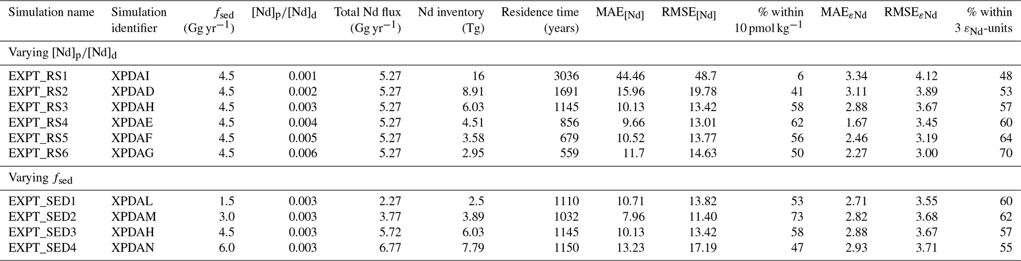
Due to time constraints, all sensitivity experiments presented here were run in parallel. First, $[\mathrm{Nd}{]}_{\mathrm{p}}/[\mathrm{Nd}{]}_{\mathrm{d}}$ is systematically varied in six sensitivity simulations ($[\mathrm{Nd}{]}_{\mathrm{p}}/[\mathrm{Nd}{]}_{\mathrm{d}}$ ranging 0.001–0.006), these values are based upon results from similar modelling schemes (Rempfer et al., 2011; Arsouze et al., 2009; Gu et al., 2019) and consider the few direct observations of $[\mathrm{Nd}{]}_{\mathrm{p}}/[\mathrm{Nd}{]}_{\mathrm{d}}$ (Jeandel et al., 1995; Stichel et al., 2020; Zhang et al., 2008; Paffrath et al., 2021; Bertram and Elderfield, 1993; Tachikawa et al., 1999). Here, based upon simulations undertaken when validating the scheme and estimates from previous optimised Nd isotope schemes (Arsouze et al., 2009; Rempfer et al., 2011; Gu et al., 2019; Pöppelmeier et al., 2020a), f_sed is fixed at 4.5 Gg yr⁻¹ throughout.

Second, f_sed is varied in four sensitivity simulations (f_sed ranging 1.5–6.0 Gg yr⁻¹), using values based upon previous recent estimates of a global sediment flux to seawater (3.3–5.5 Gg yr⁻¹; Gu et al., 2019; Pöppelmeier et al., 2020b; Rempfer et al., 2011) and encompassing a larger parameter space in order to explore the sensitivity of Nd distributions. Notably, our f_sed sensitivity studies alter the percentage contribution of the sediment Nd flux to the total Nd flux to seawater from 66 % (where f_sed=1.5 Gg yr⁻¹) to 89 % (where f_sed=6.0 Gg yr⁻¹). In all simulations $[\mathrm{Nd}{]}_{\mathrm{p}}/[\mathrm{Nd}{]}_{\mathrm{d}}$ is fixed at 0.003, which is in the middle of the range (0.001–0.006) discussed above. Following the $[\mathrm{Nd}{]}_{\mathrm{p}}/[\mathrm{Nd}{]}_{\mathrm{d}}$ sensitivity experiment (Sect. 3.1), it is apparent that 0.004 would have been a better choice for $[\mathrm{Nd}{]}_{\mathrm{p}}/[\mathrm{Nd}{]}_{\mathrm{d}}$, and we propose this as a starting point for further performance refinement in subsequent work.

Dissolved seawater Nd in all simulations is initialised from zero and integrated for at least 9000 years under constant pre-industrial boundary conditions to allow the deep-ocean circulation and marine Nd cycle to reach steady state, which we define as being when the Nd inventory becomes (near) constant with time (<0.02 % change per 100 years). All the presented results refer to or show the centennial mean from the end of the 9000-year simulations.

3 Results and discussion

3.1 Model sensitivity to reversible scavenging efficiency ($[\mathrm{Nd}{]}_{\mathrm{p}}/[\mathrm{Nd}{]}_{\mathrm{d}}$)

The first set of sensitivity experiments tests the response of simulated [Nd]_d and ε_Nd to a systematic variation in the reversible scavenging tuning parameter ($[\mathrm{Nd}{]}_{\mathrm{p}}/[\mathrm{Nd}{]}_{\mathrm{d}}$). Despite total Nd flux to seawater being fixed, varying the scavenging efficiency ($[\mathrm{Nd}{]}_{\mathrm{p}}/[\mathrm{Nd}{]}_{\mathrm{d}}$) leads to different Nd inventories (see Fig. 9 and Fig. S7 in the Supplement for the percentage rate of change per 100 years) and residence times (Table 3), consistent with previous studies (Siddall et al., 2008; Arsouze et al., 2009; Rempfer et al., 2011; Gu et al., 2019). A higher $[\mathrm{Nd}{]}_{\mathrm{p}}/[\mathrm{Nd}{]}_{\mathrm{d}}$ increases both the Nd scavenging efficiency and removal via sedimentation by enabling a larger fraction of seawater Nd to adsorb onto particles, in turn leading to a lower Nd inventory and a lower residence time (where; residence time is equal to Nd inventory and total Nd flux).

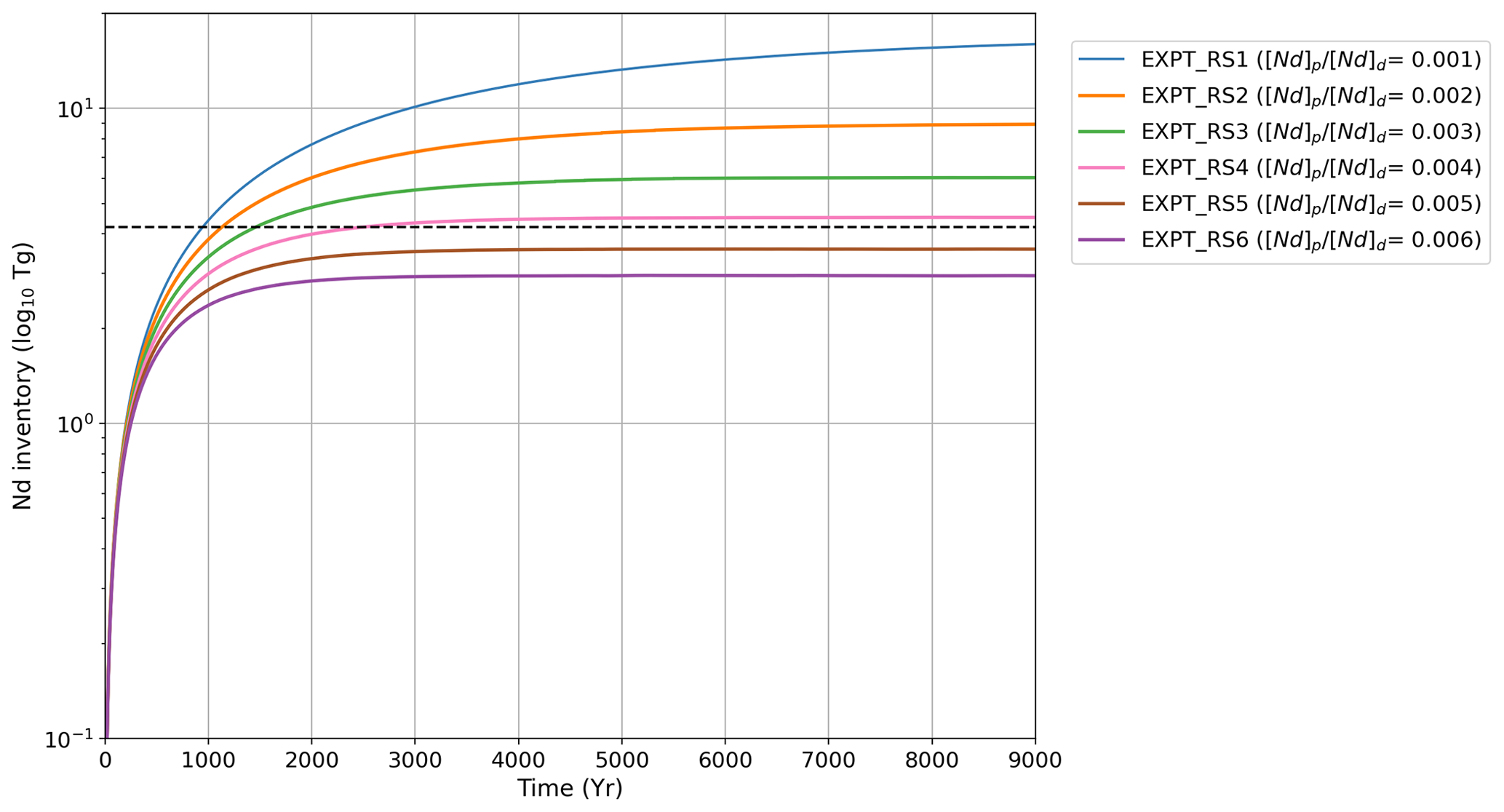
Figure 9 Global Nd inventory (g) simulated with different values for the reversible scavenging tuning parameter, $[\mathrm{Nd}{]}_{\mathrm{p}}/[\mathrm{Nd}{]}_{\mathrm{d}}$, as indicated. Dashed line represents the estimated global marine Nd inventory of 4.2 × 10¹² g by Tachikawa et al. (2003) used as a first-order target for our simulations.

By year 6000, experiments EXPT_RS3–EXPT_RS5 reach steady state. We therefore deem these simulations to have reached an acceptable equilibrium state. We explain why EXPT_RS1, EXPT_RS2, and EXPT_RS6 do not reach equilibrium below, but this is also because of their unrealistic condition after 9000 years. For example, EXPT_RS1 and EXPT_RS2 reach an Nd inventory far above the target inventory of 4.2 Tg (Tachikawa et al., 2003), while the high sink in EXPT_RS6 causes imbalances in surface [Nd]_d (which tends towards zero). As a result, these simulations are largely omitted from further discussion and analysis.

Neodymium in EXPT_RS1, which has the lowest $[\mathrm{Nd}{]}_{\mathrm{p}}/[\mathrm{Nd}{]}_{\mathrm{d}}$, has a residence time of 3036 years. This is much larger than the global ocean overturning time of 1500 years, resulting in an Nd inventory of 16 Tg after 9000 years. The $[\mathrm{Nd}{]}_{\mathrm{p}}/[\mathrm{Nd}{]}_{\mathrm{d}}$, and consequently the sink in EXPT_RS1, is too small to balance the input of Nd from the sources, causing such high Nd to accumulate in the simulation, which as a result does not reach steady state (rate of change 0.16 % per 100 years at the end of the simulation; Fig. 9). Thus, EXPT_RS1 returns the largest MAE_[Nd] and MAE_εNd from these simulations, indicating the worst model–data fit, especially for representing [Nd]_d measurements. EXPT_RS6, the simulation with the largest $[\mathrm{Nd}{]}_{\mathrm{p}}/[\mathrm{Nd}{]}_{\mathrm{d}}$, returns the lowest MAE_εNd. However, the sink term is too strong, resulting in a Nd inventory of 2.95 Tg, and the simulation fails to reach steady state (rate of change 0.07 % per 100 years by the end of the run). On balance, we surmise that EXPT_RS4 has the most reasonable combination of prognostic skill in terms of simulated Nd inventory (4.51 Tg) and residence time (856 years). This simulation, with $[\mathrm{Nd}{]}_{\mathrm{p}}/[\mathrm{Nd}{]}_{\mathrm{d}}$ of 0.004, shows the best balance between Nd accumulation and removal, and hence returns the lowest MAE_[Nd] alongside a moderately well-performing MAE_εNd that falls in the middle of the range of results.

In contrast to our model, the schemes by Rempfer et al. (2011) and Gu et al. (2019) required a lower $[\mathrm{Nd}{]}_{\mathrm{p}}/[\mathrm{Nd}{]}_{\mathrm{d}}$ of 0.001 and 0.0009, respectively, for their optimised experiment with Nd inventories of ≈4.2 Tg. Despite having similar scavenging schemes, a direct comparison of the parameter values used in the different Nd isotope modelling studies is difficult to make. This is because the divergence in sensitivity to reversible scavenging efficiency can be attributed to a combination of the differing magnitude and spatial distributions of model biogeochemical particle fields and Nd inputs, which are also partly controlled by the different architecture and horizontal resolution of the physical models. We thus propose that a future modelling protocol for intercomparing different global Nd isotope schemes would be well suited to exploring these differing sensitivities comprehensively.

The different values of MAE_[Nd] and MAE_εNd across our sensitivity experiments (Table 3) illustrate the distinctive and uncoupled behaviour of [Nd]_d and ε_Nd within the ocean, as broadly described by the Nd paradox, indicating that different processes govern the global distributions of each.

Generally, simulated [Nd]_d distributions in EXPT_RS4 match observational data well (Fig. 10). The lowest concentrations occur in the surface layers, and deep-water [Nd]_d increases along the global circulation pathway and with increasing age of water masses (Bertram and Elderfield, 1993; van de Flierdt et al., 2016; Tachikawa et al., 2017). Thus, we may infer that the model scheme in FAMOUS does have the broad capability of representing the physical and biogeochemical processes governing global marine [Nd]_d distributions. However, the scheme does tend to overestimate the global vertical [Nd]_d gradient with depth (see Fig. 10 and Fig. S9 in the Supplement for major ocean basin averaged depth profiles), a feature reported in previous similar model schemes (e.g. Arsouze et al., 2009; Gu et al., 2019), indicating that the representation of processes governing vertical [Nd]_d does not yet fully capture all processes occurring in the ocean. This overestimated vertical [Nd]_d gradient with depth could be a result of the simplified uniform particle settling rate applied, which may be too high in the upper layers (due to lower settling velocities in the surface mixed layer resulting from enhanced turbulence and complexation with organic ligands; Chamecki et al., 2019; Noh et al., 2006) and too low at depth (due to higher settling velocities from particle aggregation).

Figure 10 Maps of [Nd]_d (left column) and ε_Nd (right column) in simulation EXPT_RS4 split into four different depth bins: (a–b) shallow (0–200 m), (c–d) intermediate (200–1000 m), (e–f) deep (1000–3000 m), and (g–h) deep abyssal ocean (>3000 m). Water column measurements from within each depth bin (Osborne et al., 2017, 2015; GEOTRACES Intermediate Data Product Group, 2021) are superimposed as filled circles using the same colour scale.

Too high simulated [Nd]_d at depth may also be caused by the benthic sediment source being too strong, coupled with the simplified assumption of a globally uniform sediment flux acting across the entire seafloor. This suggests that perhaps too much emphasis has been put on a widespread abyssal benthic flux to resolve the Nd paradox, and it may be that shallower and marginal regions pose a larger in magnitude and more distinct Nd source to seawater as opposed to an open-ocean benthic source. Recent pore water measurements by Deng et al. (2022) on the East China continental shelf revealed larger benthic fluxes across the dynamic hydraulic environment of the continental shelf compared to deep pore water, which acted as a sink, likely due to authigenic precipitation. As such, spatial variations in the benthic flux are likely affected by multiple complex depth-related processes, although deep-ocean regions may still dominate the total area-integrated benthic flux. A future evolution of the scheme could explore depth-dependent benthic flux rates.

Moreover, the overestimation of [Nd]_d at depth could be a result of biases within the simulated biogenic particle fields. Comprehensive global observations of sinking particles fluxes – the central driver of ocean biogeochemical cycling – remain fundamentally difficult to obtain (Dunne et al., 2007), and our particle fluxes may be inaccurate as a consequence (see Sect. 2.3.4 for assumptions and respective limitations). It also seems likely that the reversible scavenging parameterisations, which are simple by design due to incomplete understanding (also Sect. 2.3.4), restrict the model's ability to precisely capture all aspects of the measured Nd distributions. For example, we know that the assumption of a globally uniform $[\mathrm{Nd}{]}_{\mathrm{p}}/[\mathrm{Nd}{]}_{\mathrm{d}}$ is oversimplified, as particle measurements suggest $[\mathrm{Nd}{]}_{\mathrm{p}}/[\mathrm{Nd}{]}_{\mathrm{d}}$ is not uniform in seawater (Stichel et al., 2020). High remineralisation rates, inducing increased exchange, have been observed in the Labrador Sea (Lagarde et al., 2020), whilst vast expanses of low biological productivity in the Pacific gyres mean [Nd]_p levels are generally much lower here compared to the North Atlantic. Thus, the global $[\mathrm{Nd}{]}_{\mathrm{p}}/[\mathrm{Nd}{]}_{\mathrm{d}}$ in our scheme may be skewed towards lower values. Nonetheless, it is necessary to adopt a pragmatic approach for the model development, and hence (similar to other model schemes) the globally uniform $[\mathrm{Nd}{]}_{\mathrm{p}}/[\mathrm{Nd}{]}_{\mathrm{d}}$ remains in our implementation. Future work could explore regionally varied $[\mathrm{Nd}{]}_{\mathrm{p}}/[\mathrm{Nd}{]}_{\mathrm{d}}$, which would benefit from additional measurement constraints to sufficiently justify a more complex distribution. Additionally, other particles such as Fe and Mn oxides and hydroxides that are not considered here may play an important role in scavenging of Nd (e.g. Bayon et al., 2004; Lagarde et al., 2020; Du et al., 2022). Further observational evidence of the processes involved and their importance for Nd cycling by combined particulate and dissolved measurements and laboratory experiments (e.g. Stichel et al., 2020; Pearce et al., 2013; Rousseau et al., 2015; Wang et al., 2021; Paffrath et al., 2021; Lagarde et al., 2020), plus experimentation within a modelling framework, may help to improve this limitation.

However, the largest model–data disparities for [Nd]_d occur in the shallow ocean (above 200 m) at specific locations close to continental margins where Nd is input to the ocean through major point sources that are not well resolved by the model. This includes continental margins in the Labrador Sea (where simulated [Nd]_d is 3 pmol kg⁻¹ compared to measured [Nd]_d of 70 pmol kg⁻¹) and the Sea of Japan (where simulated [Nd]_d is 2 pmol kg⁻¹ compared to measured [Nd]_d of 50 pmol kg⁻¹). Such low [Nd]_d in the surface layers may be exacerbated by operational constraints in the scheme, such as the extensive and immediate dilution of point-sourced Nd across the whole of its containing grid cell combined with the instantaneous nature of simulated reversible scavenging, which may be much faster in the model than would occur normally. Furthermore, the scheme may be underestimating the magnitude of surface sources of Nd, for example the Nd sourced from dust may be too low in certain regions, possibly resulting from the globally fixed (2 %) solubility of Nd from dust sources applied. In the preliminary optimisation of the Nd isotope scheme in the GNOM v1.0 model, Pasquier et al. (2022) found that dust solubility needed to be increased to unrealistically high levels to best fit measurements; for example, the optimised parameter for North American dust solubility was 83 %. A future exploration of the regional solubility and amount of Nd coming from dust sources would be needed to explore this in detail. On the other hand, recent evidence suggests that there may be a major particulate riverine flux of Nd to the ocean (Rousseau et al., 2015; Rahlf et al., 2021), which implies that the magnitude of the sediment Nd sourced to seawater near river mouths could be too weak. Specific to our scheme, the vertical convection of water from the physical ocean model in FAMOUS may also be too intense in the North Atlantic, leading to surface underestimations of [Nd]_d and overestimations at depth; a re-tuning of the physical model would help to ascertain the extent to which this limitation contributes towards the simulated Nd bias.

Nonetheless, consistent with compilations of water column measurements (Tachikawa et al., 2017; van de Flierdt et al., 2016), overall global distributions of simulated ε_Nd are broadly most non-radiogenic in the North Atlantic and more radiogenic in the North Pacific (Fig. 10), with intermediate values in the Southern and Indian oceans. The most non-radiogenic ε_Nd occurs in the surface layers of the Hudson Bay and Labrador Sea regions, and they closely match measured data (${\mathit{\epsilon }}_{\mathrm{Nd}}=-\mathrm{18}$). However, the most radiogenic ε_Nd, simulated in the surface layers of marginal regions in the North Pacific and equatorial western Pacific (${\mathit{\epsilon }}_{\mathrm{Nd}}=-\mathrm{3}$), is significantly lower than measured (${\mathit{\epsilon }}_{\mathrm{Nd}}=+\mathrm{3}$). In the central and North Pacific, particularly above 1000 m, simulated ε_Nd is −7, but measurements are closer to −1. At the basin scale, the magnitude of the ε_Nd gradient from Pacific to Atlantic is underestimated by the model and presents a familiar bias when compared to previous Nd isotope schemes (Arsouze et al., 2009; Rempfer et al., 2011; Pöppelmeier et al., 2020a; Jones et al., 2008; Gu et al., 2019). This is mainly due to the simulated Pacific being too non-radiogenic (basinal mean ε_Nd of −7.5) compared to measured water samples (${\mathit{\epsilon }}_{\mathrm{Nd}}=-\mathrm{4}$), while simulated and measured basinal mean Atlantic ε_Nd values are in much better agreement (${\mathit{\epsilon }}_{\mathrm{Nd}}=-\mathrm{11}$ and −12.5, respectively; Supplement Fig. S9). Possible explanations for why our simulated Pacific ε_Nd is so much lower than what has been recorded in modern seawater include that the model boundary conditions, specifically the marine sediment source of Nd (taken directly from Robinson et al., 2021), may not be sufficiently radiogenic or that the sediment flux from the seafloor is not uniform; points we will return to later (Sect. 3.2).

Simulated [Nd]_d with depth at distinct locations in all the reversible scavenging sensitivity experiments (Fig. 11a–f and h–m) generally (though not always) exhibit similar depth profiles to the observational data. The best model–data fit is seen within depth profiles in the Pacific and Southern oceans and notably more so under higher $[\mathrm{Nd}{]}_{\mathrm{p}}/[\mathrm{Nd}{]}_{\mathrm{d}}$. The largest model–data offsets across all sensitivity experiments in terms of both the magnitude and the depth gradients in [Nd]_d occur in the North Atlantic Ocean. In particular, the large near-surface concentrations are not resolved, with the largest disparities occurring under higher scavenging parameterisations.

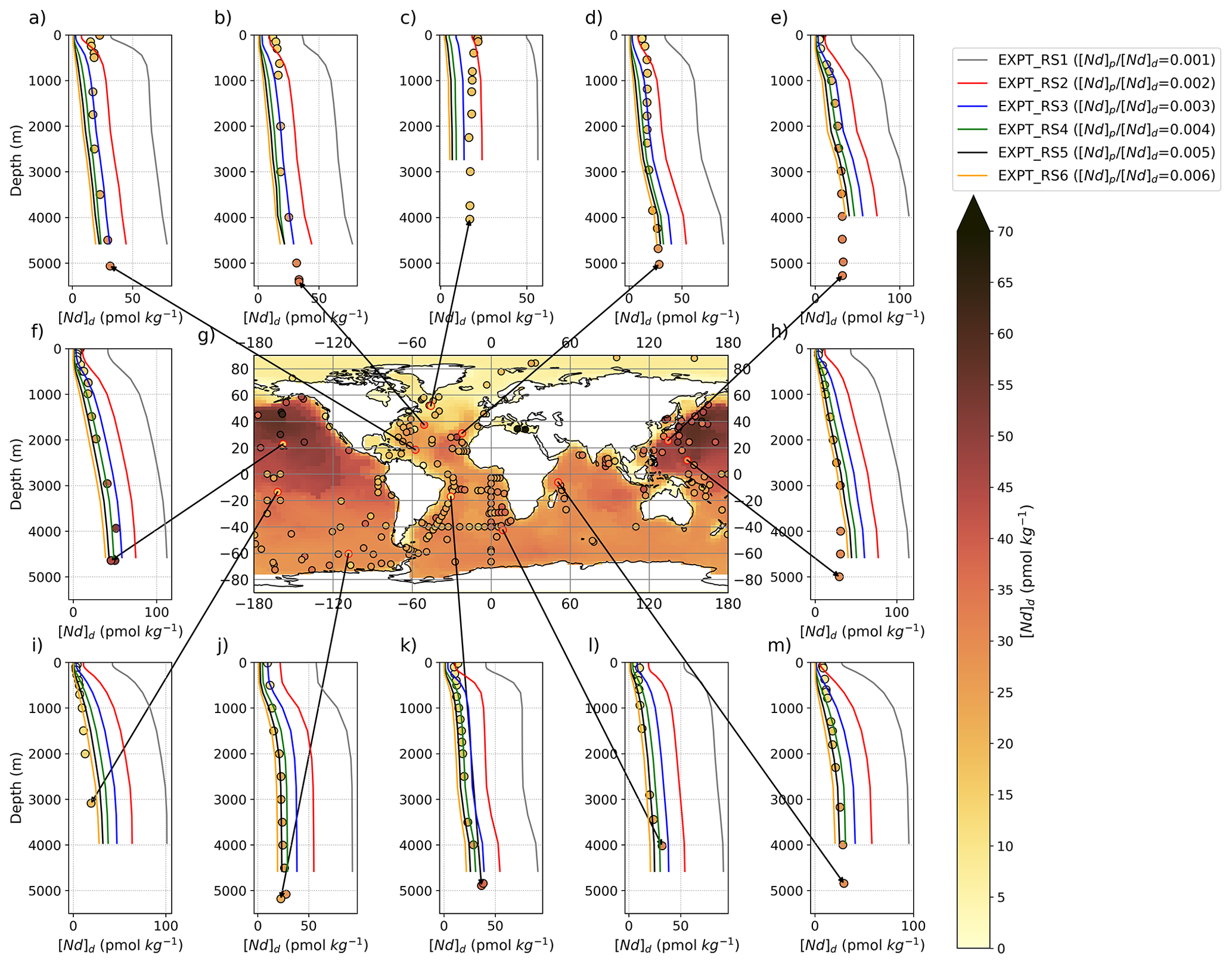
Figure 11 The central panel (g) displays [Nd]_d at the seafloor (i.e. lowermost box of the ocean model) in simulation EXPT_RS4 (100-year mean from the end of the run), with superimposed water column measurements (Osborne et al., 2017, 2015; GEOTRACES Intermediate Data Product Group, 2021) from ≥3000 m shown by filled coloured circles on the same colour scale. The surrounding panels (a)–(f) and (h)–(m) display depth profiles of simulated (coloured lines, one per sensitivity simulation with varied $[\mathrm{Nd}{]}_{\mathrm{p}}/[\mathrm{Nd}{]}_{\mathrm{d}}$) and measured (filled circles) [Nd]_d, respectively. Larger shifts in the [Nd]_d between simulations highlight the regions most sensitive to the efficiency of reversible scavenging.

For ε_Nd, the response to varying scavenging efficiency has varied effects across depths and between ocean regions, indicating a more complex relationship between how reversible scavenging can delineate global ε_Nd distributions in comparison to [Nd]_d. Increased scavenging efficiency traps regional ε_Nd provenance signals, resulting in larger inter-basin ε_Nd gradients, the strength of which are favoured by the combination of strong scavenging efficiency and a short seawater residence time. Although the simulated ε_Nd profiles with depth do not closely follow measurements, it is valuable to discuss the sensitivity of simulated ε_Nd to variations in scavenging efficiency. The North Atlantic is the most sensitive basin to changes in reversible scavenging (registered by the greater ε_Nd profile shifts between different experiments, Fig. 12a–d), particularly at depths below 2000 m, indicating that reversible scavenging, alongside convection at sites of deep-water formation, are important processes for governing the simulated ε_Nd signal of deep-water masses. Thus, a stronger reversible scavenging efficiency is needed to set the non-radiogenic deep ocean signature in the North Atlantic and to trap these regional ε_Nd provenance signals locally.

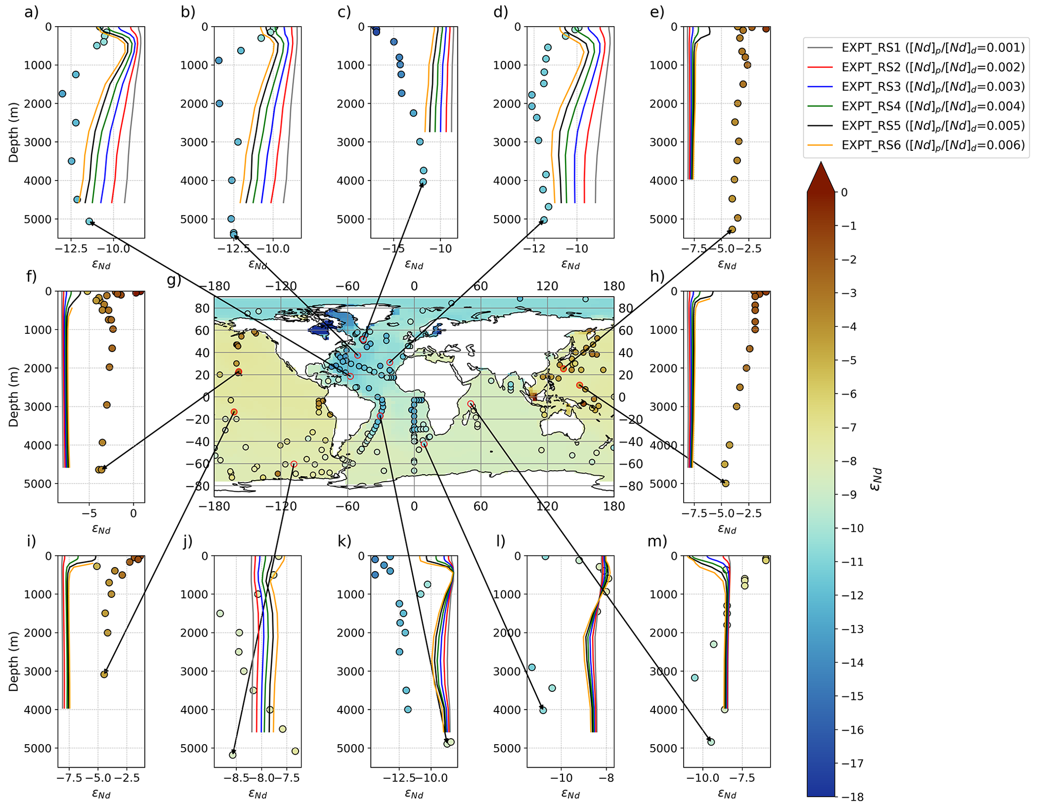
Figure 12 The central panel (g) displays ε_Nd at the seafloor (i.e. lowermost box of the ocean model) in simulation EXPT_RS4 (100-year mean from the end of the run), with superimposed water column measurements (Osborne et al., 2017, 2015; GEOTRACES Intermediate Data Product Group, 2021) from ≥3000 m shown by filled coloured circles on the same colour scale. The surrounding panels (a)–(f) and (h)–(m) display depth profiles of simulated (coloured lines, one per sensitivity simulation with varied $[\mathrm{Nd}{]}_{\mathrm{p}}/[\mathrm{Nd}{]}_{\mathrm{d}}$) and measured (filled circles) ε_Nd, respectively. Larger shifts in the ε_Nd between simulations highlight the regions most sensitive to the efficiency of reversible scavenging.

Typical depth profiles from measurements in the subtropical North Atlantic show contrasts in ε_Nd that co-vary with the presence of major water masses (coloured circles in Fig. 12a–b). Across all sensitivity experiments, there is relative consistency with depth for the profiles in the subtropical North Atlantic (e.g. Fig. 12b), ranging from −10 to −12 under increasing scavenging efficiency, which acts to drive more localised non-radiogenic signals. This simulated uniformity may be due to the indiscriminate seafloor sedimentary flux here being too high and thereby dominating the deep seawater ε_Nd signal. An additional explanation may be due to the lack of abyssal (i.e. below 3 km) AABW, which does not extend past ∼ 20^∘ N (Fig. 3). This insufficient AABW production and penetration into the Atlantic are known limitations of FAMOUS (Dentith et al., 2019; Smith, 2012), although these biases are reduced in our control compared to the previous studies (Sect. 2.2). Thus, the seawater below the surface mixed layer comprises only North Atlantic water, and in so doing the model will not resolve the AABW signal inferred from measurements at depth in higher latitudes.

Higher up the water column, the more non-radiogenic NADW seen in the seawater measurements is conspicuously absent (note the ε_Nd minima in subtropical North Atlantic measurements ∼ 1000–2000 m deep, Fig. 12a–b), even though we know NADW does reside there in the model (see Fig. 3 for verification). We may relate this to the high-latitude North Atlantic ε_Nd being too radiogenic to tag NADW with its characteristically non-radiogenic ε_Nd signal, particularly around the mouth of the Labrador Sea (Fig. 10a–b). This could be exacerbated by a dampening of the non-radiogenic NADW ε_Nd from a relatively radiogenic seafloor benthic flux along the water flow path (Fig. 6). Consequently, despite a close correlation to seawater ε_Nd in the subtropics and lower NADW (where measurements of ε_Nd are −12.4 and simulated is −12), the upper NADW end-member ε_Nd is not sufficiently non-radiogenic, even under the highest reversible scavenging efficiency ([Nd]_p/[Nd]_d=0.006), where simulated ε_Nd is −12, which is in contrast to seawater records of −13.2 ε_Nd (Lambelet et al., 2016).

In contrast, ε_Nd in the Pacific Ocean is least sensitive to changes in $[\mathrm{Nd}{]}_{\mathrm{p}}/[\mathrm{Nd}{]}_{\mathrm{d}}$, particularly below 500 m (Fig. 12e–f, h–i). This is expected due to the absence of major ocean convection and ventilation, meaning the Pacific contains an older and more homogenised pool of water in comparison to the Atlantic, and thus water masses are far less distinct and the localised ε_Nd signal does not get dispersed via convection as rapidly. The deep seafloor-wide sediment source governs simulated ε_Nd distributions in the intermediate to deep Pacific due to its larger flux relative to that transported vertically via particle scavenging and dissolution or horizontally by the sluggish convection of the Pacific. One further aspect to note is that in some Pacific regions [Nd]_d in the surface layers tends towards zero under a high sink ([Nd]_p/[Nd]_d=0.006). This causes numerical instabilities in modelled Nd ratios, and thus ε_Nd is meaningless where [Nd]_d<0.2 pmol kg⁻¹ and is therefore masked out of the results shown by Fig. 12 to avoid misinterpretation.

The simulated depth profile in all experiments in the Indian Ocean matches the observed intermediate ε_Nd signal of −8 between 500 and 2000 m (Fig. 12m). However, the more radiogenic ε_Nd signal of −6 in the surface layers is not captured and neither is the shift in ε_Nd below 2000 m to more non-radiogenic values reaching a minimum of −10.5 at 3000 m, with all experiments simulating a relatively uniform ε_Nd with depth. Under higher reversible scavenging parameters for this depth profile (EXPT_RS4–EXPT_RS6), the surface concentrations are too low (simulated [Nd]_d=3 pmol kg⁻¹; observed [Nd]_d=8 pmol kg⁻¹), indicating that the model is not fully resolving either the concentration or the ε_Nd from a surface flux here and that scavenging may be too intense at the surface. In the deeper ocean (≈3000 m), these simulations show the model represents the [Nd]_d profiles better but is missing an non-radiogenic exchange of ε_Nd at depth. This could point to an non-radiogenic sediment source or exchange that is misrepresented by the bulk sediment boundary conditions and sediment source assumptions (e.g. our application of a global seafloor sediment source of Nd irrespective of sedimentary characteristics).

In the Southern Ocean, simulations with $[\mathrm{Nd}{]}_{\mathrm{p}}/[\mathrm{Nd}{]}_{\mathrm{d}}$ ≥0.003 broadly match the general measured ε_Nd at depths above 1000 m (decreasing with depth from −7.8 at the surface to −8.2 at 1000 m). Below this (and down to 3000 m), observed diversions in ε_Nd are not captured in any of the sensitivity experiments. This discrepancy can be attributed to the simulation of quite homogenous AABW throughout the water column in the region, which represents a physical bias of FAMOUS (Dentith et al., 2019; Smith, 2012). Specifically, in the Pacific sector of the Southern Ocean (Fig. 12j), the model cannot resolve the measured non-radiogenic spike at 1500 m, which captures the distinct presence of lower Circumpolar Deep Water (CDW, ${\mathit{\epsilon }}_{\mathrm{Nd}}=-\mathrm{8.4}$ ± 1.6: Lambelet et al., 2018) formed from mixing of Atlantic-, Pacific-, and Indian-sourced waters.

Thus, we conclude that scavenging and removal via sedimentation is necessary to balance the simulated input sources and enables the scheme to reach equilibrium around reasonable Nd inventories. We find that reversible scavenging is an important process that enhances the ε_Nd gradient between oceans by maintaining localised basinal ε_Nd signals throughout the water column. The strength of this process is particularly important for maintaining the simulated non-radiogenic ε_Nd in the well-ventilated North Atlantic Ocean (alongside deep-water formation) but less important for the more stagnant modern Pacific Ocean.

Nonetheless, parameterising reversible scavenging efficiency alone cannot account for the correct trends and magnitude within ε_Nd gradients observed between basins and in depth profiles. Currently, the scheme assumes that all particles reaching the seafloor via reversible scavenging are buried in the sediment and as such are decoupled from the seafloor sediment source, whereas there is no Nd release and the particles are removed from the model. A future evolution of the scheme could explore the dissolution of authigenic sedimentary phases on the seafloor during diagenesis to investigate how this may influence the ε_Nd distributions of the benthic flux. Moreover, our results demonstrate the importance of further constraining other aspects of marine Nd cycling under a holistic framework. Furthermore, we note that the scheme described here may not be fully resolving the end-member ε_Nd of different water masses due to an imperfect representation of the sources of Nd to seawater (i.e. the model boundary conditions and strength of the source fluxes). Thus, in some instances, the scheme carries inappropriate or dampened ε_Nd signals, coupled alongside particular structural model biases in the physical circulation (e.g. limited AABW intrusion in the North Atlantic). Although in the case of the latter point, we note that this is not a limitation of the presented scheme and that the implementation can be useful for identifying such physical biases.

3.2 Model sensitivity to Nd flux from the sediment (f_sed)

The second set of sensitivity simulations tests the response of [Nd]_d and ε_Nd to systematically varying the total Nd flux from the sediment (f_sed). In this experiment, Nd accumulates rapidly from the start of the simulations (Fig. 13 and Supplement: Fig. S8 for the percentage rate of change per 100 years) and tapers off thereafter to varying degrees depending on the rate of accumulation. By year 6000 all f_sed sensitivity experiments have reached steady state (<0.02 % change per 100 years).

Figure 13 Global Nd inventory (Tg) simulated with different values for the total sediment flux tuning parameter (f_sed) as indicated. The dashed line represents the estimated global marine Nd inventory of 4.2 Tg from Tachikawa et al. (2003) used as an approximate target for the simulations. Note the logarithmic scale on the y axis.

Modifying the sediment flux while keeping the sink term $[\mathrm{Nd}{]}_{\mathrm{p}}/[\mathrm{Nd}{]}_{\mathrm{d}}$ constant returns a varied equilibrium Nd inventory across the suite of simulations (Fig. 13). However, without changing the scavenging efficiency (i.e. Nd sink), there is a more moderate range of 40 years difference in the f_sed simulations' Nd residence time (Table 3). In general, the relatively low scavenging efficiency of all of the f_sed sensitivity simulations ($[\mathrm{Nd}{]}_{\mathrm{p}}/[\mathrm{Nd}{]}_{\mathrm{d}}=\mathrm{0.003}$; see Sect. 3.1 for context) yields long residence times greater than 1000 years.

EXPT_SED1, which has the lowest f_sed, corresponding to a sediment flux (per area) of 1.17 pmol cm² yr⁻¹, and hence the lowest total Nd flux to the ocean, returns the smallest total Nd inventory of 2.5 Tg (Table 3). Conversely, EXPT_SED4, which has the largest f_sed, corresponding to a sediment flux of 4.69 pmol cm² yr⁻¹, results in the greatest Nd inventory (7.8 Tg), producing both the worst MAE_[Nd] and worst MAE_εNd.

We note that compared to varying the reversible scavenging efficiency, varying f_sed drives relatively small changes in Nd distributions, as demonstrated by the minor differences in MAE_εNd between sensitivity experiments. This makes sense since varying f_sed only acts to change the fractional contribution from each specific Nd source, e.g. an enhanced f_sed reduces the fraction of total Nd flux coming from dust and rivers (which are inputs constrained to the surface and point sources close to the continents), concentrating the flux across the global seafloor (and vice versa). However, in all simulations and consistent with previous studies, the sediment Nd source to seawater remains the major source, and f_sed would need to be reduced much more to greatly influence MAE_εNd.

Overall, from the simulations in this study, EXPT_SED2 demonstrates the best skill for [Nd]_d compared to measurements, returning the lowest MAE_[Nd]of 7.96 pmol kg⁻¹ (Table 3) and achieving the most balanced Nd source and sink terms. Although the simulation does not represent the lowest MAE_εNd, the range across the f_sed experiment is small (2.71 to 2.93; Table 3), and it does simulate the highest percentage of simulated ε_Nd within 3 ε_Nd units of measurements (62 %). The sediment flux in EXPT_SED2 of 2.35 pmol cm² yr⁻¹ is considered similar to the few existing measurements of a benthic flux across different sedimentary environments, which are mostly on the order of 10 pmol cm² yr⁻¹ (Abbott, 2019; Abbott et al., 2015a; Haley et al., 2004; Du et al., 2018). In comparison with model estimates of the benthic flux, the sediment flux in EXPT_SED2 is most comparable to the global benthic flux estimated by Pöppelmeier et al. (2020a) of 5.4 pmol cm² yr⁻¹ but an order of magnitude lower than the value of 20–30 pmol cm² yr⁻¹ estimated by Du et al. (2020). Alternatively, the depth scaling of the benthic flux in the modelling study by Pasquier et al. (2022) resulted in surface fluxes of 83.7 pmol cm² yr⁻¹ and deep-ocean fluxes of 1.11 pmol cm² yr⁻¹.

The target global Nd inventory of 4.2 Tg, derived from the canonical work by Tachikawa et al. (2003), is based on a sparser array of seawater measurements, particularly in the Southern Ocean, compared to what is available today. Using our newer compilation of [Nd]_d to identify the best-performing simulation for [Nd]_d (EXPT_SED2), we can report an updated estimate of the global Nd inventory from the model of 3.89 Tg (Table 4), noting that this is likely an underestimate of the total since the model does not represent marginal seas. Furthermore, we can examine the basinal distribution of [Nd]_d, (also Table 4), whereby the largest amount is found in the stagnant North Pacific, where the greatest area-integrated sediment flux occurs. Smaller Nd inventories are found in the more convective North Atlantic and Southern Ocean regions, which have less expansive seafloors and larger biogenic particle fluxes, resulting in more Nd removal via reversible scavenging and sedimentation. We propose that future work should take advantage of the greater abundance of seawater Nd measurements (e.g. as compiled in this study) to produce a detailed update to the estimate of oceanic inventories of Nd. These more accurate Nd budgets across diverse ocean regions and depths would help in improving constraints on the marine Nd cycle and would provide excellent model evaluation tools.

Table 4 Nd inventory (Tg) for EXPT_SED2 within different ocean regions.

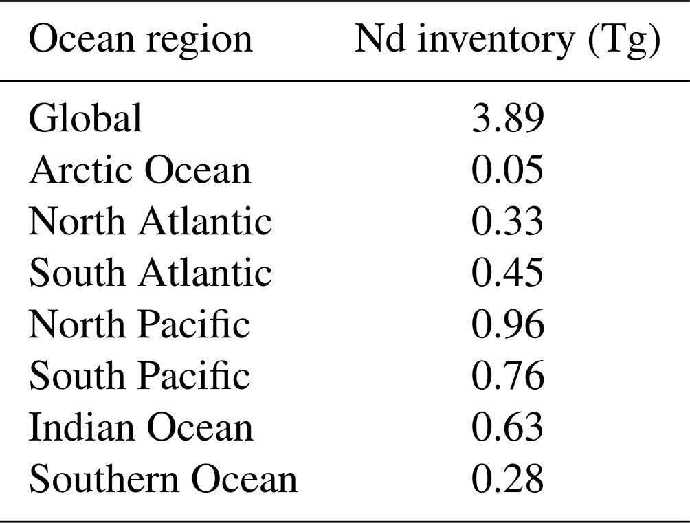
Altogether, simulated [Nd]_d in EXPT_SED2 matches the general observational data trend of Nd concentration. However, in the deep layers of the North Pacific (below 3000 m) simulated [Nd]_d is underestimated (36 pmol kg⁻¹ compared to 50 pmol kg⁻¹ from seawater measurements). This underestimation of [Nd]_d at depth can be explained by a combination of having a seafloor sediment source at the lower end of our range (f_sed is 3.0 Tg yr⁻¹) and slow release from reversible scavenging ($[\mathrm{Nd}{]}_{\mathrm{p}}/[\mathrm{Nd}{]}_{\mathrm{d}}$ of 0.003; our experiments suggest 0.004 may be a more suitable efficiency to use, Sect. 3.1), highlighting the importance of both non-conservative processes in governing deep [Nd]_d distributions.

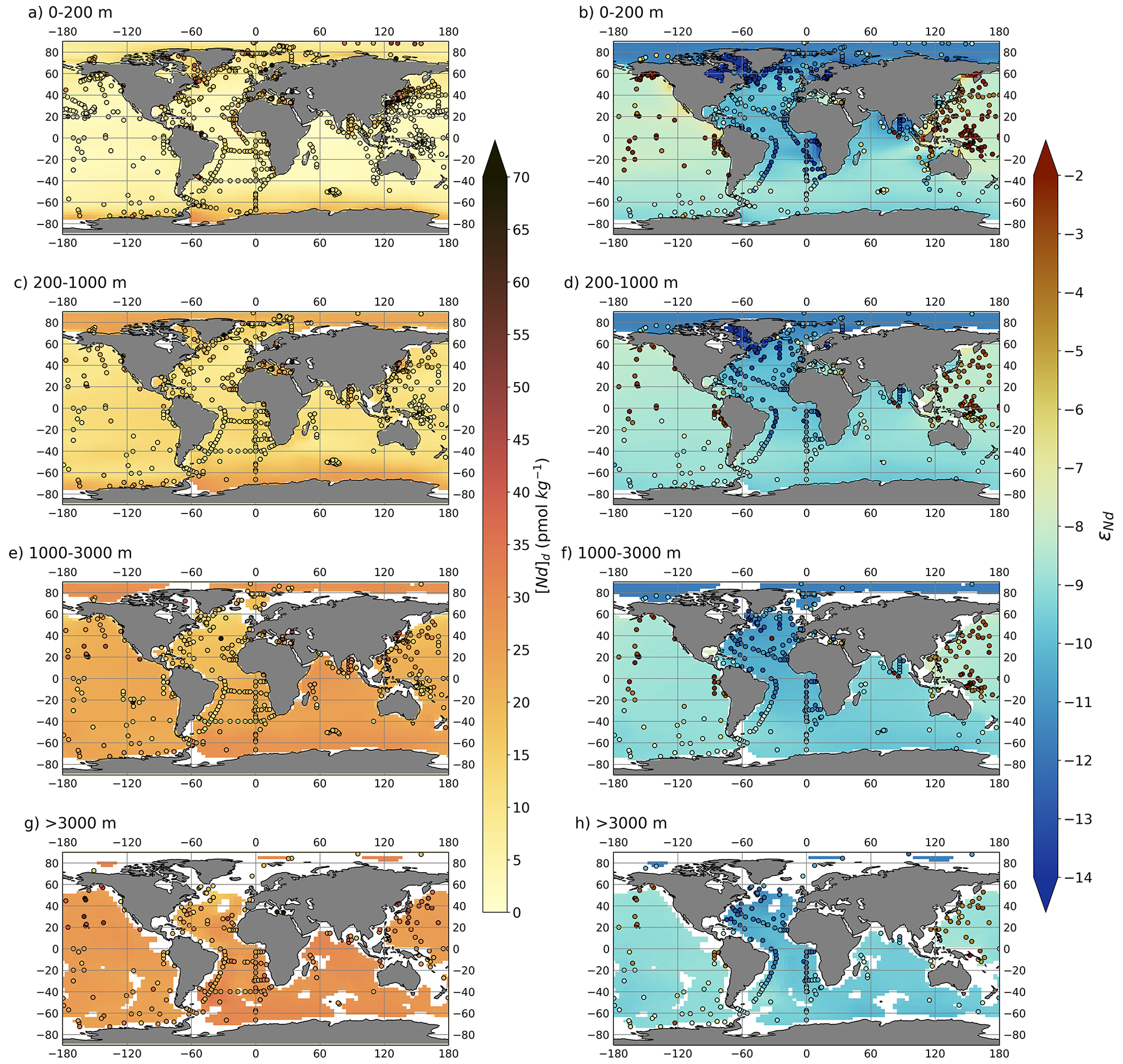
Figure 14 Maps of [Nd]_d (left) and ε_Nd (right) in simulation EXPT_SED2 split into four different depth bins: (a–b) shallow (0–200 m), (c–d) intermediate (200–1000 m), (e–f) deep (1000–3000 m), and (g–h) deep abyssal ocean (>3000 m). Water column measurements from within each depth bin (Osborne et al., 2017, 2015; GEOTRACES Intermediate Data Product Group, 2021) are superimposed as filled circles using the same colour scale.

Moreover, the longer lifetime of simulated Nd in the EXPT_SED2 ocean (1032 years) compared to that estimated by previous work (360–800 years; Gu et al., 2019; Rempfer et al., 2011; Siddall et al., 2008; Tachikawa et al., 2003) means that Nd becomes well mixed in the deep ocean (below 1000 m), homogenising the ε_Nd signal. This causes the observed inter-basin gradients (a critical feature in the use of Nd as an ocean circulation tracer) to become severely damped, particularly away from direct input of fresh reactive phases with distinctive ε_Nd (Robinson et al., 2021; Abbott et al., 2019). Consistent with earlier studies (e.g. Arsouze et al., 2009; Jones et al., 2008), the largest model–data disparities occur in the North Pacific and equatorial Pacific, where simulated ε_Nd is far too non-radiogenic compared to the observational data, pointing to a number of processes that may be better optimised in our Nd scheme. For example, a larger (and also more radiogenic) sediment source (i.e. greater f_sed) may be needed, particularly around shallow to intermediate marginal settings, which is a suggestion also supported by the too low [Nd]_d.

Total Nd concentrations and isotopic distributions show different responses to varying f_sed. We find that [Nd]_d is sensitive to f_sed across all ocean basins (i.e. a wide divergence in the depth profiles shown in Fig. 15), mostly at depths below 500 m where there is no direct influence from river and dust inputs and the relatively large area of the deep abyssal seafloor as an Nd interface becomes important (particularly with low reversible scavenging).

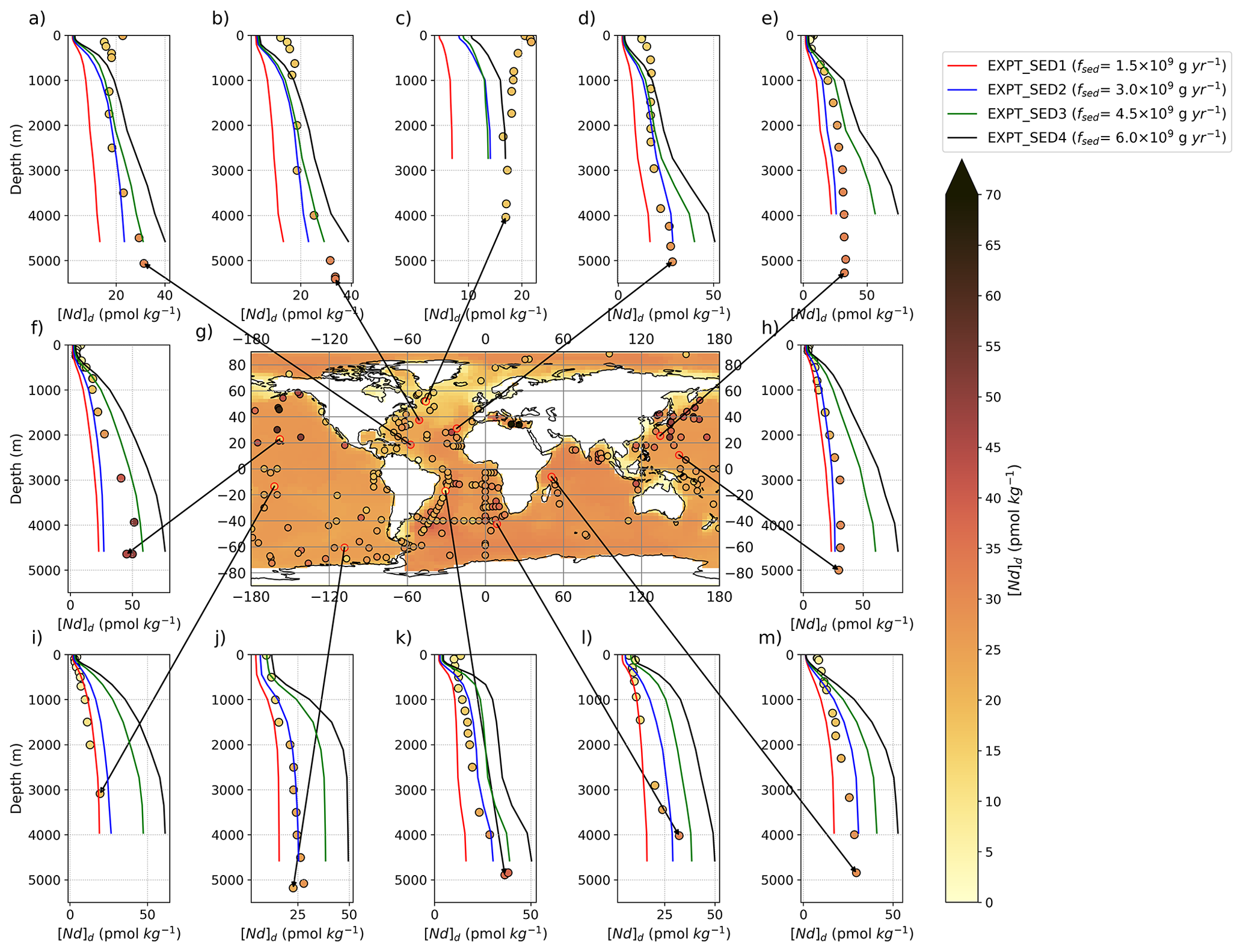
Figure 15 The central panel (g) displays [Nd]_d at the seafloor (i.e. lowermost box of the ocean model) in simulation EXPT_SED2 (100-year mean from the end of the run), with superimposed water column measurements (Osborne et al., 2017, 2015; GEOTRACES Intermediate Data Product Group, 2021) from ≥3000 m shown by filled coloured circles on the same colour scale. The surrounding panels (a)–(f) and (h)–(m) display depth profiles of simulated (coloured lines, one per sensitivity simulation with varied f_sed) and measured (filled circles) [Nd]_d, respectively. Larger shifts in the [Nd]_d between simulations highlight the regions most sensitive to the magnitude of the seafloor sediment source.

Typically, the best model–data fit for [Nd]_d depth profiles is achieved under lower f_sed (1.5 to 3.0 Gg yr⁻¹) and in the Pacific, Indian, and Southern oceans in particular (Fig. 15). Correspondingly, under high f_sed and in the deeper interior of the ocean in particular (below 3000 m), simulated [Nd]_d diverges to higher concentrations than measured due to too much Nd being sourced to the deep ocean from the sediment. Additionally, in these high f_sed scenarios, the strength of the deep sediment source obscures horizontal seafloor [Nd]_d gradients across basins (see the near-uniform seafloor [Nd]_d in Fig. 15g), masking the influence of reversible scavenging, which is controlled by the location and dissolution of particle fields and is important for governing [Nd]_d patterns (Sect. 3.1).

Similar to the reversible scavenging sensitivity experiment (Sect. 3.1), the largest simulated offsets between simulated and measured [Nd]_d under all f_sed experiments occur in the North Atlantic and subtropical Atlantic at depths above 1000 m, where, even under the largest sediment fluxes, simulated [Nd]_d is too low. The depth profile south of Greenland (Fig. 15c) shows the greatest sensitivity to varying f_sed in the upper 1000 m, with EXPT_SED4's simulated surface concentrations of 10 pmol kg⁻¹ (f_sed=6.0 Gg yr⁻¹) being closest to the measured concentrations of 22 pmol kg⁻¹. By implication, the accurate representation of sediment fluxes is required to reproduce upper-ocean [Nd]_d in this region, and an enhanced sediment flux alone cannot account fully for the observed high surface concentrations. Either the combination of the surface and near-surface fluxes resolved here is too diluted in the model (possibly due to grid box resolution) or the model is missing a significant surface or near-surface Nd source. Previous schemes have likewise simulated too low surface [Nd]_d in the North Atlantic, likely also due to difficulties in representing highly localised and variable surface features in global models (Gu et al., 2019; Rempfer et al., 2011); more direct observations of surface fluxes would benefit future constraints in this region.

Whereas [Nd]_d is sensitive to f_sed globally, the height of ε_Nd sensitivity is more regional (Fig. 16). The Atlantic, Indian, and Southern oceans have ε_Nd values that are significantly more sensitive to changes in the bulk seafloor sediment Nd flux than the Pacific Ocean. Overall, differences in f_sed tend to drive whole depth profile shifts of low magnitude in ε_Nd. This contrasts the findings of Rempfer et al. (2011), who varied a margin-constrained f_sed and reported that deep-water ε_Nd (below 1000 m) values were affected less than in our results. If this conflicting difference in deep-ocean sensitivity to f_sed is because of the applied spatial distributions of a sediment Nd source to seawater (<3000 m for Rempfer et al., 2011, and all depths for this study), then further constraints on sediment Nd fluxes across space and time are crucial when interpreting ocean circulation from ε_Nd.

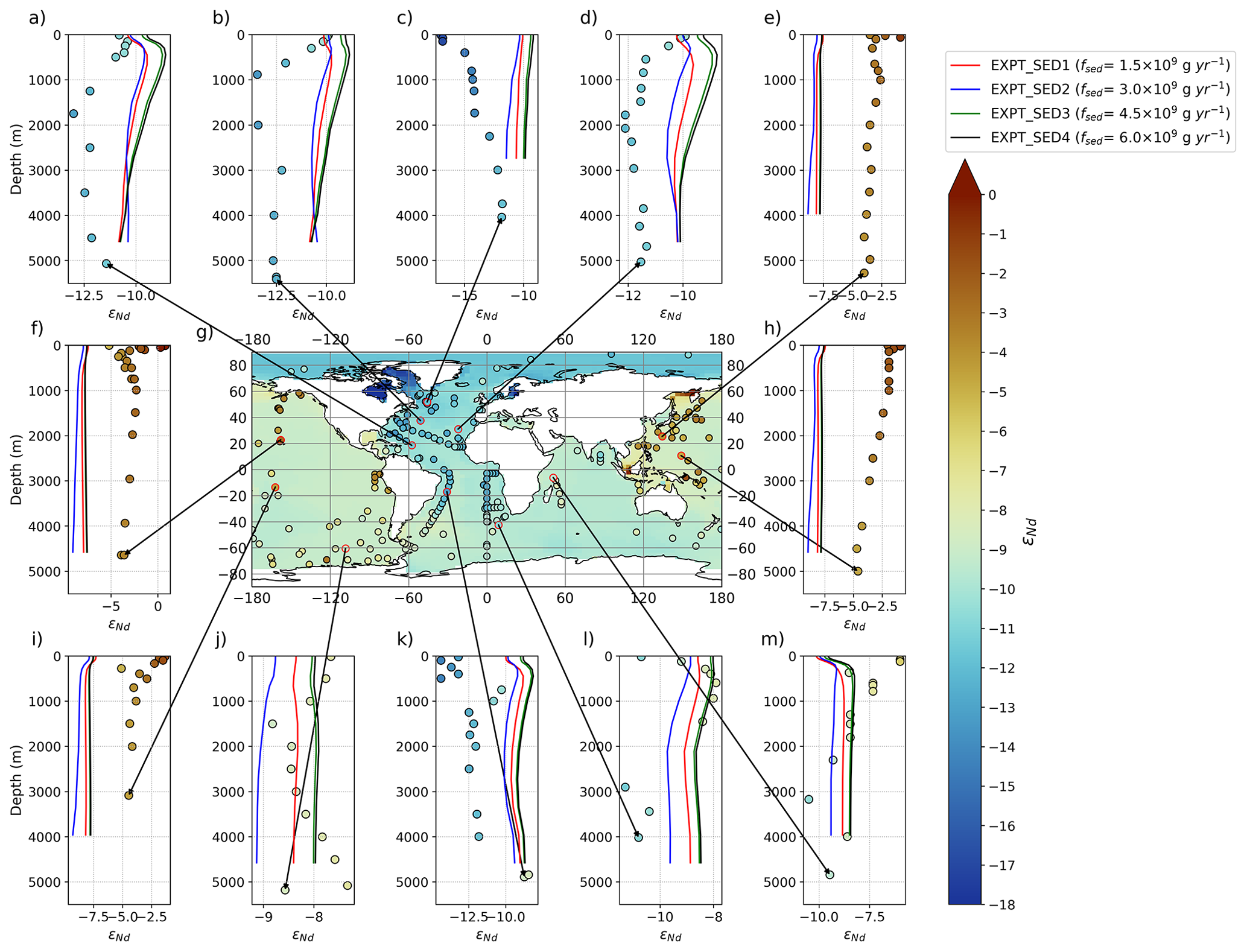
Figure 16 The central panel (g) displays ε_Nd at the seafloor (i.e. lowermost box of the ocean model) in simulation EXPT_SED2 (100-year mean from the end of the run), with superimposed water column measurements (Osborne et al., 2017, 2015; GEOTRACES Intermediate Data Product Group, 2021) from ≥3000 m shown by filled coloured circles on the same colour scale. The surrounding panels (a)–(f) and (h)–(m) display depth profiles of simulated (coloured lines, one per sensitivity simulation with varied f_sed) and measured (filled circles) ε_Nd, respectively. Larger shifts in the ε_Nd between simulations highlight the regions most sensitive to the magnitude of the seafloor sediment source.

Once again, the most notable ε_Nd model–data mismatch occurs within the depth profiles of the North Atlantic. Due to major rivers delivering a high [Nd] load to the Atlantic (Fig. 5c) in their vicinity, simulations with low f_sed are conditioned towards riverine ε_Nd, providing the typical non-radiogenic ε_Nd signature of NADW (Fig. 16a–d). Conversely, enhancing f_sed increases the fraction of Nd supplied to the ocean from the bulk seafloor sediment, which has more uniform, intermediate ε_Nd values in the central North Atlantic (−12.5) in contrast to the more non-radiogenic ε_Nd signals of the continental margins and riverine source in the Labrador (−28) and West Atlantic basins (−15.6), with localised near-surface sediment extreme minimums of −34 in the northern Labrador Sea (Robinson et al., 2021). Greater f_sed thus acts to overprint and hence mix away the more distinct surface ε_Nd signal of NADW gained at their sites of deep-water formation in favour of a more general intermediate ε_Nd signal as it becomes exposed to Nd fluxes along its southward seafloor flow path. Model–measurement disparity at the mouth of the Labrador Sea and south of Greenland suggests that a specific fraction of the bulk sediment with more non-radiogenic ε_Nd than is captured by Robinson et al. (2021) may be driving particle–seawater interactions (Fig. 17). Mechanical glacial erosion, which exposes large amounts of highly non-radiogenic and labile fine-grained crystalline detritus in the region surrounding the Labrador Sea likely drives enhanced localised extreme non-radiogenic benthic fluxes (Von Blanckenburg and Nägler, 2001; Anderson, 2005). Moreover, marine particle ε_Nd measured in the North Atlantic has been shown to reflect the strong heterogeneity of the surrounding source rock, for example the provenance of extremely radiogenic particles (+6 to +9) at the Irminger Basin has been associated with mafic rocks found in eastern Greenland and Iceland (Stichel et al., 2020). It therefore follows that better spatial constraints on sediment fluxes are required for providing accurate ε_Nd tagging of Atlantic seawater.

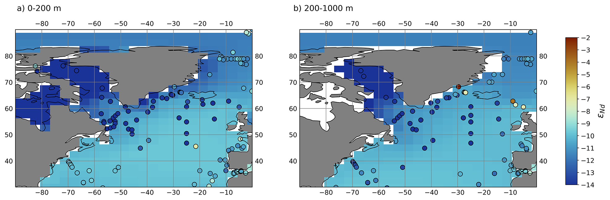
Figure 17 Volume-weighted distributions of ε_Nd in simulation EXPT_SED2 split into two different depth bins, (a) shallow (0–200 m) and (b) intermediate (200–1000 m), within the North Atlantic and Labrador Sea basins. Water column measurements from within each depth bin (Osborne et al., 2017, 2015; GEOTRACES Intermediate Data Product Group, 2021) are superimposed as filled circles on the same colour scale. Note that Iceland is not resolved in FAMOUS (Jones, 2003).

In contrast to the Atlantic, the Pacific Ocean ε_Nd is the least sensitive to varying f_sed (Fig. 16e–f, h–i). Characteristically, the Pacific encompasses vast open-ocean oligotrophic expanses with low biogenic particle export, in tandem with smaller relative dust and river sources, which means the seafloor sediment source already dominates the simulated Nd fluxes and distributions, even under lower sediment fluxes. In the North Pacific, the ε_Nd signal from the bulk seafloor sediment cannot explain the radiogenic ε_Nd observed here (Fig. 16), and thus the model is likely not fully capturing the correct source (or the prescribed boundary condition is not correctly representing the distribution and fraction of the sediment phase contributing to the sediment flux) of Nd to seawater. Authigenic precipitation of clay minerals during reverse weathering is prevalent in the pelagic sediment throughout the North Pacific. These top centimetres of sediment are typically assumed to be unreactive and act as an active sink for REE (Kato et al., 2011). Moreover, precipitation at hydrothermal vents also acts as an effective localised REE sink (German et al., 1990). Therefore, the red clays of the deep Pacific may act as an effective Nd sink and not a source. Alternatively, a recent reactive transport model by Du et al. (2022) suggests reverse weathering maintains under-saturation of primary silicates in deep Pacific pore water, driving enhanced silicate weathering and favouring preferential dissolution of highly radiogenic volcanic sediments (e.g. basaltic glass and clinopyroxene). Here, we highlight the need for more precise constraints on complex benthic processes in the Pacific, including exploring the environmental conditions that would drive spatially elevated and “reactivity-weighted” sediment fluxes.

To conclude, we surmise that a sediment–seawater flux represents a key major source of [Nd]_d that is particularly fundamental to the intermediate and deep-ocean Nd budgets and as such plays an important role in governing marine Nd cycling. Indeed, a strong seafloor-wide uniform sediment source pushes the ocean towards a more globally uniform and too high [Nd]_d than measurements from the deep ocean suggest. This could be interpreted as evidence against a globally widespread benthic-flux-driven model of the marine Nd cycle with a spatially constant flux across diverse sedimentary environments in favour of the more distinct [Nd]_d distributions that may be achieved under a model of marine Nd cycling with larger and more heterogenous surface and near-surface Nd sources and a greater dominance of reversible scavenging. Future work should explore employing a more horizontally nuanced benthic flux tied to local environmental and sedimentary conditions, in line with recent modelling studies (Pöppelmeier et al., 2020a; Pasquier et al., 2022), to introduce more spatial patterning in simulated [Nd]_d.

Certainly, these sensitivity simulations demonstrate that (at least under a spatially uniform benthic flux) the bulk ε_Nd of seafloor detrital sediment (Robinson et al., 2021) cannot be considered fully representative of the ε_Nd composition of the sediment that is interacting with seawater in all instances. They highlight the need for observational and experimental quantification of the broad mobile Nd phases globally and their ε_Nd signal, as well as constraints on the spatial distribution of such a benthic flux (e.g. identifying where and under what environmental conditions a benthic flux occurs and at what strength). The model's response to f_sed sets the stage for further testing of global sedimentary ε_Nd on marine Nd cycling, providing the foundation for resolving the inherent complex multitude of processes.

4 Summary and conclusions

In this study, we describe the implementation of Nd isotopes (¹⁴³Nd and ¹⁴⁴Nd) into the ocean component of the FAMOUS GCM (Nd v1.0), providing a powerful tool designed for comprehensively exploring global marine Nd cycling, especially through representing explicit non-conservative processes to explore the extent of their influence on global seawater Nd distributions. Our Nd isotope scheme starts from previous Nd isotope implementations (Rempfer et al., 2011; Gu et al., 2019; Pöppelmeier et al., 2020a; Arsouze et al., 2009; Siddall et al., 2008) but revisits and updates Nd sources, sinks, and tracer transformation in line with increased observations and recent findings relating to global marine Nd cycling.

Model sensitivity to reversible scavenging efficiency demonstrates its importance for determining the increase in Nd concentration along the circulation pathway and acts to enhance regional basinal gradients in simulated ε_Nd by maintaining the localised provenance signal. On the other hand, a widespread seafloor sedimentary flux presents a major deep-ocean source of Nd, the magnitude of which governs horizontal seafloor Nd concentrations across ocean basins. In the deep North Pacific, simulated ε_Nd is too non-radiogenic compared to measurements, highlighting that the ε_Nd of the sediment flux, as captured by the bulk ε_Nd, is not a true representation of the highly radiogenic labile sediment phase interacting with seawater. Moreover, authigenic precipitation may pose a missing effective Nd sink. Model–data mismatch at the mouth of the Labrador Sea suggests that detrital contributions from highly non-radiogenic sediments disproportionally govern particle–seawater interactions. Overall, our results demonstrate that more precise constraints are needed to resolve the complex benthic processes that would drive spatially elevated and reactivity-weighted sediment fluxes.

Exploring the behaviour of simulated [Nd]_d and ε_Nd distributions in detail also highlighted some of the structural limitations of the model (e.g. difficulties representing highly localised and surface features) and influential biases in the physical ocean circulation (e.g. limited northward intrusion of AABW in the North Atlantic).

This study provides the groundwork for a future comprehensive optimisation of the marine Nd isotope scheme in FAMOUS. In the first instance, we suggest calibration of the key tuning parameters ($[\mathrm{Nd}{]}_{\mathrm{p}}/[\mathrm{Nd}{]}_{\mathrm{d}}$ and f_sed) to best represent modern seawater measurements. Additionally, it would be beneficial to obtain additional observational constraints on the broad labile sediment ε_Nd interacting with seawater across different seafloor regions, including constraining the exchange between authigenic and detrital sediment phases during early diagenesis. Future sensitivity studies could also focus on the influence of river particulate and continental marginal sources on marine Nd to provide further insight into (and possibly constrain) the relative importance of these inputs, as opposed to a predominantly benthic seafloor-wide source.

This new model scheme can aid in the delivery of more robust applications of ε_Nd as a modern and palaeo-tracer. It provides a platform for dynamic modelling under different modes of marine Nd cycling or varied climatic and oceanographic conditions, enabling current hypotheses to be tested rigorously with the aim of constraining Nd cycling under a complex and partially understood marine geochemical system.