Using the two-way nesting technique AGRIF with MARS3D V11.2 to improve hydrodynamics and estimate environmental indicators

In the ocean, mesoscale or submesoscale structures and coastal processes are associated with fine scales. The simulation of such features thus requires the hydrodynamic equations to be solved at high-resolution (from a few hundred meters down to a few tens of meters). Therefore, local mesh refinement is a primary issue for regional and coastal modeling. The AGRIF (adaptive grid refinement in Fortran) library is committed to tackling such a challenge for structured grids. It has been implemented in MARS3D (Model for Application at Regional Scale), a semi-implicit, free-surface numerical model developed by Ifremer (the French Research Institute for Exploitation of the Sea) for coastal environmental research and studies. As its time scheme uses an alternating-direction implicit (ADI) algorithm, the two-way nesting implementation differs from the one in explicit models. The present paper describes the specifics of the AGRIF introduction and how the nesting preserves some essential properties (mass, momentum and tracer conservations) along with the induced constraints (bathymetric coherence between grids and increase in computation cost). The use and the performance of this new tool are detailed over two configurations that illustrate the wide range of scales and resolutions typically targeted by coastal applications. The first one is based on multiple high-resolution (500 m) grids that pave the coastal ocean over thousands of kilometers, allowing a continuum between the regional and coastal scales. The second application is more local and has a finer resolution (50 m). It targets a recurrent question for semi-enclosed bays, i.e., the renewal time indicator. Throughout these configurations, the paper intends to compare the two-way nesting method with the traditional one-way approach. It highlights how the MARS3D-AGRIF tool proves to be an efficient way to both improve the physical hydrodynamics and unravel ecological challenges.

1 Introduction

In the ocean, many observations have clearly shown that turbulence is ubiquitous and that flows are turbulent at all scales (Capet, 2015). It is also admitted that capturing the whole range of oceanic scales is far beyond the capabilities of any numerical model for a long time to come. Indeed, the large-eddy simulation (LES) approach dedicated to solving the direct forward-turbulent energy cascade is far from being reachable, except for strict localized places. Therefore, it is necessary to develop relevant and efficient parameterizations at the subgrid scale and propose refinement capabilities in ocean models to focus the computational grid at key locations. A key region can vary considerably based on geographic or dynamical considerations. As the circulation is obviously tightly controlled by the coastline and more generally by the bathymetry, increasing the resolution of the grid may be essential to properly catch the coastal morphology (e.g., estuaries, capes, peninsulas and small bays and lagoons). Alternatively, a key region may be where critical processes take place and determine the circulation or fate of a coastal discharge, even when far offshore. The Strait of Gibraltar, where internal jumps and, consequently, internal solitary wave trains are generated, is a perfect illustration, as these features propagate for hundreds of kilometers (Naranjo et al., 2014) until they break and reinforce mixing. Thus, the generating area must be addressed with both sufficient resolution and even locally adapted physics (here non-hydrostatic) to reproduce such structures. Then they must be accurately propagated, possibly outside the refined area.

Multiple strategies can be investigated (and are available with some degree of efficiency and accuracy) to tackle the spatial refinement in limited areas. A first strategy relies on unstructured grids together with finite volume or finite element discretizations; numerous models such as Delft3D (Roelvink and van Banning, 1995), SLIM (Delandmeter et al., 2018), TELEMAC-3D (Janin et al., 1993) or T-UGOm (Piton et al., 2020) have shown their capability to cope with complex geometrical features such as river deltas or continental slope for years. A second strategy is based on curvilinear, either orthogonal (Rétif et al., 2014; Diaz et al., 2020; Marsaleix et al., 2006; among many others) or non-orthogonal (Grasso et al., 2018), grids. However, the design of such grids might be a great deal of work and have a lack of flexibility.

These approaches have also raised classical issues related to continuously adaptive subgrid parameterization with regards to how to manage both temporal and spatial refinements so that the computational cost required by the finest-scale grid cells does not spill over to the entire grid. Recently, Li (2021) proposed a 2D shallow-water mode discretized on a regional spherical multiple cell which circumvents this constraint. An alternative method applies to structured grids and provides a refinement capability (adaptive or not) to recursively integrate a hierarchy of grids at different resolutions. This kind of approach was proposed in the early 1980s (Berger and Oliger, 1984) and has already been implemented in either academic works (Penven et al., 2006; Debreu et al., 2012) or for large-scale realistic applications (Biastoch et al., 2009; Marchesiello et al., 2011) to improve the resolution and hence the realism of the local dynamics.

Such an approach, the adaptive grid refinement in Fortran (AGRIF; Debreu et al., 2008), is based on domain decomposition and needs the partial overlapping of same-level grids. It is expected to facilitate the offshore continuum for coastal applications, despite the overlapping constraint. Therefore, the AGRIF software has been introduced into MARS3D (Lazure and Dumas, 2008), a numerical model dedicated to coastal environmental applications. The main challenge was related to the semi-implicit time scheme. The two-way nesting is now fully operational for mass, momentum and tracer conservation. Implemented along the coasts of the northwestern European shelf and over coastal bays, the mesh refinement should allow the representation of a large spectrum of spatial (small bays and large areas) and temporal (as fast as tides or surges and as slow as mesoscale or frontal instabilities) scales.

This paper aims to demonstrate the capabilities and benefits of the two-way nesting method for modeling the interplay of coastal and regional dynamics. Section 2 describes the recent developments in the hydrodynamic model MARS3D with the AGRIF library and addresses the running performance. Afterward, two applications are presented. Section 3 depicts a regional model configuration and focuses on the systematic refinement capability. Section 4 introduces a focused coastal configuration to highlight two-way nesting improvements. Finally, these results and perspectives are discussed in Sect. 5.

2 Innovative developments for two-way nesting

2.1 The MARS3D model (v11.2 released in March 2018)

The hydrodynamic MARS3D (Model for Application at Regional Scale) model solves the primitive equations under the Boussinesq and hydrostatic assumptions. It uses finite differences over a staggered Arakawa C grid with a vertical generalized-sigma coordinate framework. It relies on a barotropic–baroclinic-mode splitting. The barotropic mode, which obeys the shallow-water equation systems, is treated with a modified alternating-direction implicit (ADI) algorithm (Leendertse and Gritton, 1971). Unlike split explicit free-surface models, the temporal integration of both barotropic and baroclinic modes is carried out with the same time step due to a wider stability range of the barotropic mode. The barotropic–baroclinic coupling is simplified, but the propagation of the barotropic mode is weaker as the scheme is implicit.

Figure 1 Schematic domain decomposition for solving the ADI equation system.

The original time scheme described in Lazure and Dumas (2008) for MARS3D v6 has been significantly modified. This is done, first, by adding a prediction step (assessment of depth-averaged velocity ${\stackrel{\mathrm{‾}}{v}}^{n+\mathrm{1},\ast }$) and, second, by alternating the sweep of the computational grid in a row–column-wise manner and then column–row-wise manner. These modifications have been introduced to limit the spatial split errors inherent in single time step schemes. The row–column-wise form is developed in Eq. (1). It consists of computing (depth-averaged velocity ${\stackrel{\mathrm{‾}}{u}}^{n+\mathrm{1}}$ and sea surface elevation ${\mathit{\eta }}^{n+\mathrm{1},\ast }$) and then (${\stackrel{\mathrm{‾}}{v}}^{n+\mathrm{1}}{\mathit{\eta }}^{n+\mathrm{1}}$) in the first half of a time step. The second half of a time step, which symmetrically gives (${\stackrel{\mathrm{‾}}{v}}^{n+\mathrm{1}}{\mathit{\eta }}^{n+\mathrm{1},\ast }$) first and then gives (${\stackrel{\mathrm{‾}}{u}}^{n+\mathrm{1}}{\mathit{\eta }}^{n+\mathrm{1}}$) is not detailed. The first equation of the system is a local solver, whereas the second and the third equations solved together lead to a linear tridiagonal system whose size is twice the number of grid cells in a row because the unknown vector is made of (${\stackrel{\mathrm{‾}}{u}}^{n+\mathrm{1}}{\mathit{\eta }}^{n+\mathrm{1},\ast }$). Similarly, the fourth and fifth equations lead to a linear tridiagonal system whose size is twice the number of points in a column.

$$\begin{array}{}\text{(1)}& \begin{array}{rl}{\stackrel{\mathrm{‾}}{v}}^{n+\mathrm{1},\ast }& ={\stackrel{\mathrm{‾}}{v}}^n-g\mathrm{\Delta }t{\displaystyle \frac{\partial {\mathit{\eta }}^n}{\partial y}}+\mathrm{\Delta }t{G}_v\left(u^{n-\mathrm{1}}{v}^{n-\mathrm{1}}\right)\\ {\mathit{\eta }}^{n+\mathrm{1},\ast }& ={\mathit{\eta }}^n-\mathrm{\Delta }t\left[{\displaystyle \frac{\partial }{\partial x}}\left(h^n{\stackrel{\mathrm{‾}}{u}}^{n+\mathrm{1}}\right)+{\displaystyle \frac{\partial }{\partial y}}\left(h^n{\stackrel{\mathrm{‾}}{v}}^{n+\mathrm{1},\ast }\right)\right]\\ {\stackrel{\mathrm{‾}}{u}}^{n+\mathrm{1}}& ={\stackrel{\mathrm{‾}}{u}}^n-g\mathrm{\Delta }t{\displaystyle \frac{\partial }{\partial x}}\left(\mathit{\alpha }{\mathit{\eta }}^n+\left(\mathrm{1}-\mathit{\alpha }\right){\mathit{\eta }}^{n+\mathrm{1},\ast }\right)\\ & +\mathrm{\Delta }t{G}_u\left(u^n,v^n\right)\\ {\mathit{\eta }}^{n+\mathrm{1}}& ={\mathit{\eta }}^n-\mathrm{\Delta }t\left[{\displaystyle \frac{\partial }{\partial x}}\left(h^n{\stackrel{\mathrm{‾}}{u}}^{n+\mathrm{1}}\right)+{\displaystyle \frac{\partial }{\partial y}}\left(h^n{\stackrel{\mathrm{‾}}{v}}^{n+\mathrm{1}}\right)\right]\\ {\stackrel{\mathrm{‾}}{v}}^{n+\mathrm{1}}& ={\stackrel{\mathrm{‾}}{v}}^n-g\mathrm{\Delta }t{\displaystyle \frac{\partial }{\partial x}}\left(\mathit{\alpha }{\mathit{\eta }}^n+\left(\mathrm{1}-\mathit{\alpha }\right){\mathit{\eta }}^{n+\mathrm{1}}\right)\\ & +\mathrm{\Delta }t{G}_v\left(u^n,v^n\right)\end{array}\end{array}$$

In Eq. (1), h stands for the total water depth, Δt is the time step and α is the implicit coefficient of the external pressure gradient term. The term $G_{u/v}\left(u^n{v}^n\right)$ gathers the vertical average of all the remaining terms, including the nonlinear and the horizontal dissipation terms, the Coriolis force and the friction at the surface and the bottom. All of these remaining terms are explicit and not discussed here.

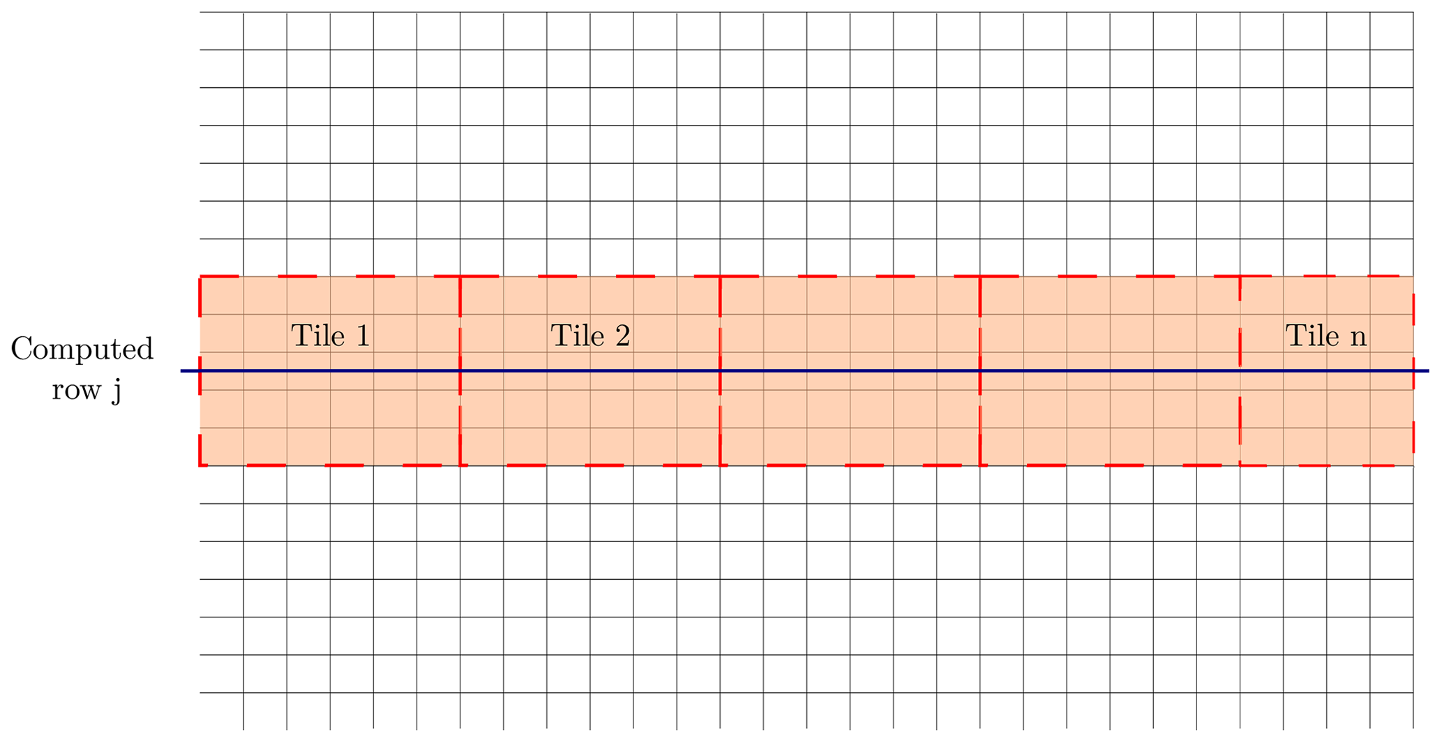
The linear tridiagonal system is a non-local solver, where ${\mathit{\eta }}^{n+\mathrm{1},\ast }$ and uⁿ⁺¹ are solved over a whole row by the ADI algorithm. Then, for a massive parallel computation based on a decomposition domain made of horizontal tiles, ηⁿ and uⁿ are distributed on the different tiles crossed by the considered row (Fig. 1). The linear system can be schematically written as diagonal blocks, where each block represents the linear tridiagonal system over a tile, as follows:

$$\begin{array}{}\text{(2)}& \begin{array}{l}\left(\begin{array}{ccc}\text{coef\hspace{0.17em} on\hspace{0.17em} tile}\mathrm{1}& \mathrm{\cdots }& \mathrm{0}\\ \mathrm{⋮}& \mathrm{\ddots }& \mathrm{⋮}\\ \mathrm{0}& \mathrm{\cdots }& \text{coef\hspace{0.17em} on\hspace{0.17em} tile}n\end{array}\right)\\ \left(\begin{array}{c}\mathit{\eta },u\text{on\hspace{0.17em} tile}\mathrm{1}\\ \mathrm{⋮}\\ \mathit{\eta },u\text{on\hspace{0.17em} tile}n\end{array}\right)\\ =\left(\begin{array}{c}rhs\text{on\hspace{0.17em} tile}\mathrm{1}\\ \mathrm{⋮}\\ rhs\text{on\hspace{0.17em} tile}n\end{array}\right).\end{array}\end{array}$$

It shows that η and u need to be gathered into a single row tile and that, once the linear tridiagonal system is solved, the solution has to be broadcasted back to the original geographic tiles. In order to reduce the communications, the first three equations of the system (1) have been rearranged into the system (3) thanks to the splitting of uⁿ⁺¹ into an explicit part and an implicit one. This leads to a tridiagonal system in which the unknown vector is made solely of ${\mathit{\eta }}_i^{n+\mathrm{1},\ast }$.

$$\begin{array}{}\text{(3)}& \begin{array}{rl}{\stackrel{\mathrm{‾}}{v}}^{n+\mathrm{1},\ast }& ={\stackrel{\mathrm{‾}}{v}}^n-g\mathrm{\Delta }t{\displaystyle \frac{\partial {\mathit{\eta }}^n}{\partial y}}+\mathrm{\Delta }t{G}_v\left(u^{n-\mathrm{1}}{v}^{n-\mathrm{1}}\right)\\ {\stackrel{\mathrm{‾}}{u}}^{n+\mathrm{1},\ast }& ={\stackrel{\mathrm{‾}}{u}}^n-g\mathrm{\Delta }t\mathit{\alpha }{\displaystyle \frac{\partial {\mathit{\eta }}^n}{\partial x}}+\mathrm{\Delta }t{G}_u\left(u^n{v}^n\right)\\ & -g\mathrm{\Delta }{t}^{\mathrm{2}}\left(\mathrm{1}-\mathit{\alpha }\right){\displaystyle \frac{\partial }{\partial x}}\left[h^n{\displaystyle \frac{\partial {\mathit{\eta }}^{n+\mathrm{1},\ast }}{\partial x}}\right]+{\mathit{\eta }}^{n+\mathrm{1},\ast }\\ & ={\mathit{\eta }}^n-\mathrm{\Delta }t\left[{\displaystyle \frac{\partial }{\partial x}}\left(h^n{\stackrel{\mathrm{‾}}{u}}^{n+\mathrm{1},\ast }\right)+{\displaystyle \frac{\partial }{\partial y}}\left(h^n{\stackrel{\mathrm{‾}}{v}}^{n+\mathrm{1},\ast }\right)\right]\\ {\stackrel{\mathrm{‾}}{u}}^{n+\mathrm{1}}& ={\stackrel{\mathrm{‾}}{u}}^{n+\mathrm{1},\ast }-g\mathrm{\Delta }t\left(\mathrm{1}-\mathit{\alpha }\right){\displaystyle \frac{\partial {\mathit{\eta }}^{n+\mathrm{1},\ast }}{\partial x}}\end{array}\end{array}$$

As a result, the length of the ADI system is now precisely the number of grid cells in the x direction for a given row, and the data involved in the message-passing interface between tiles are reduced by a factor of 2. The same methodology is applied to the fourth and fifth of system (1) in the y direction.

Figure 2 Diagram of the coupling between the barotropic and barotropic mode.

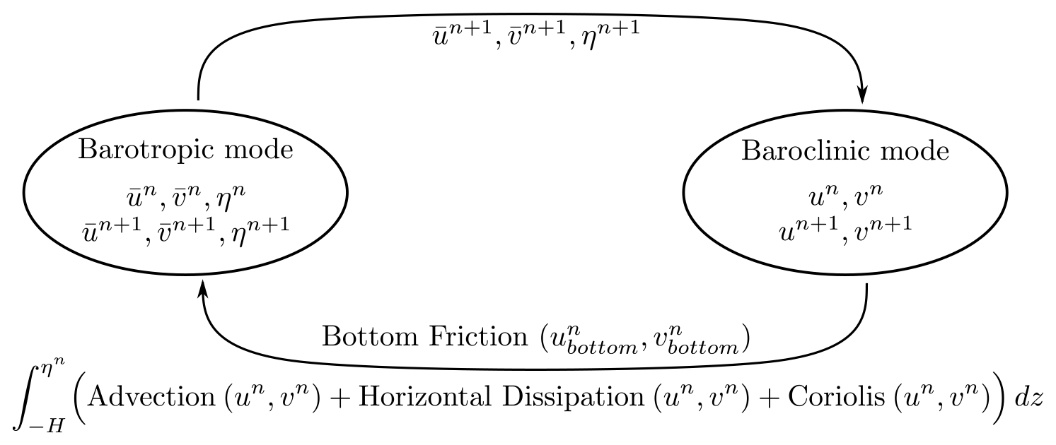
In addition to the modification of the barotropic solver itself, some additional modifications have been implemented in the barotropic–baroclinic coupling because the original iterative coupling described by Lazure and Dumas (2008) was not compatible anymore with the reformulation (3). The coupling that can be sketched (according to Fig. 2) is now straightforward. (a) The barotropic mode is forced with vertically integrated terms of advection, horizontal dissipation, Coriolis, internal pressure gradient and the bottom friction (assessed with the first level of velocity), (b) the baroclinic mode is forced with the external pressure gradient, and (c) the last classical step of the coupling consists of redistributing the vertical mismatch between the barotropic transport and the vertically integrated baroclinic transport in order to ensure mass conservation.

Last but not least, the wetting–drying capability has been modified to introduce partial drying or wetting. It consists of introducing a coefficient f_wet to the non-local continuity equation that evolves in time, according to Eq. (4):

$$\begin{array}{}\text{(4)}& \begin{array}{rl}{\mathit{\eta }}^{n+\mathrm{1}}S{f}_{\mathrm{wet}}^{n+\mathrm{1}}& ={\mathit{\eta }}^{n}S{f}_{\mathrm{wet}}^n-\mathrm{\Delta }t\left[\stackrel{\mathrm{‾}}{{\partial }_x\left(h^n{u}^{n+\mathrm{1}}\right)\mathrm{\Delta }y}\right.\\ & \left.+\stackrel{\mathrm{‾}}{{\partial }_y\left(h^n{v}^{n+\mathrm{1}}\right)\mathrm{\Delta }x}\right],\end{array}\end{array}$$

where S stands for the grid cell surface (S = ΔxΔy), and f_wet is the time-dependent fraction of the grid cell that is flooded ($\mathrm{0}\le f_{{\mathrm{wet}}_{i,j}}\le \mathrm{1}$). f_wet is given by a prognostic equation accounting for the bottom slope within the grid cell and the water column height at its center.

2.2 The AGRIF library: mesh refinement and grid interactions

AGRIF (adaptive grid refinement in Fortran; Debreu et al., 2008) is a package for the integration of structured adaptive mesh refinement (SAMR) features within a multidimensional finite difference model. Its main objective is to simplify the integration of SAMR potentialities within an existing model, while making minimal changes. In particular, it includes a lexicographic analyzer of Fortran code that generates, at the compilation step, the data structures required for running the same code on any grid hierarchy. AGRIF is currently used in the following ocean models: ROMS-AGRIF (Debreu et al., 2012; Penven et al., 2006), a regional model developed jointly at Rutgers University and University of California, Los Angeles (UCLA), the NEMO ocean modeling system (Biastoch et al., 2018, 2009), a general circulation model used by the European scientific and operational communities, and HYCOM (HYbrid Coordinate Ocean Model), a regional model developed jointly by the University of Miami and the French Navy. In MARS3D, a one-way nesting implementation ensuring only mass conservation (Muller et al., 2009) was first introduced, followed by a two-way nesting for temperature and salinity only (Dufois et al., 2014). This paper aims to introduce a comprehensive two-way nesting in accordance with the improved MARS3D time scheme, along with its evaluation in coastal environments.

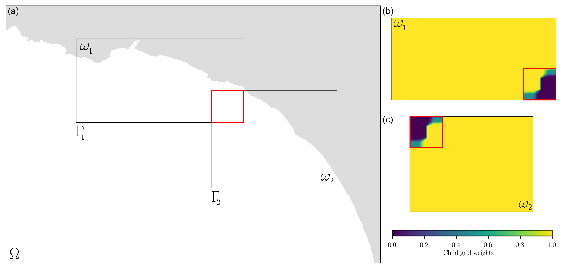
Figure 3 (a) Local refinement with two child grids. (b) The weights used for interactions at the same hierarchical level on the overlapping area are represented with a red rectangle.

2.2.1 General algorithm

For a general review of two-way nesting algorithms, the reader is referred to Debreu and Blayo (2008). This section overviews the introduction of AGRIF two-way nesting into MARS3D. The challenge was related to the implicit nature of the MARS3D time scheme, the ADI algorithm and the wetting–drying capability. Figure 3 illustrates two child grids covering the subdomains ω of the parent domain Ω. Their boundaries are delimited by the interfaces Γ. The coarse-resolution grid has a mesh size given by Δx_H, while the fine-resolution grid has a mesh size of $\mathrm{\Delta }{x}_h=\mathrm{\Delta }{x}_H/\mathit{\rho }$, where ρ is the spatial mesh refinement ratio (an integer). Subscripts H and h stand for the coarse and refined domains, respectively. The partial differential equations solved by the model can be written in the following generic forms:

$$\begin{array}{}\text{(5)}& {\displaystyle \frac{\partial q_H}{\partial t}}=L_H\left(q_H\right),{\displaystyle \frac{\partial q_h}{\partial t}}=L_h\left(q_h\right).\end{array}$$

L_H and L_h represent the same continuous operator L at the coarse (H) and fine (h) resolutions. On the child grid, equations are integrated from an initial state, which refers to the conservative spatial interpolation of the initial condition on the coarse grid. Throughout the time integration, the child grid lateral boundary conditions at the interface Γ are provided by temporal and spatial conservative interpolations from the coarse grid. In the two-way mode, the coarse resolution model is updated using the fine resolution model once the temporal integration of the fine grids is completed, i.e., after ρ_t sub-time steps. In short, this nesting uses two different operators, namely a spatiotemporal interpolator (P) and a restriction operator (R), respectively. Using an explicit convention to simplify, the algorithm can be written in the following conceptual form for a single, coarse-grid half of a time step:

1. $q_H^{n+\mathrm{1}}=L_H\left(q_H^n\right)$ (temporal integration of the coarse grid);

2. For  m = 1…ρ_t   Do

   ${\left.q_h^{n+\frac{m}{{\mathit{\rho }}_t}}\right|}_{\mathrm{\Gamma }}=P\left(q_H^n,q_H^{n+\mathrm{1}}\right)$ (computation of open boundary conditions from the coarse grid to the child grid);

   $q_h^{n+\frac{m}{{\mathit{\rho }}_t}}=L_h\left(q_h^{n+\frac{\left(m-\mathrm{1}\right)}{{\mathit{\rho }}_t}}\right)$ (temporal integration of the child grid);

3. $$\begin{array}{}\text{(6)}& \begin{array}{rl}{\left.q_H^{n+\mathrm{1}}\right|}_{\mathit{\omega }}& =R\left(q_h^{n+\mathrm{1}}\right)\text{(update of the coarse grid }\\ & \text{over the area of overlap)}.\end{array}\end{array}$$

Here, ρ_t is the time refinement factor (${\mathit{\rho }}_t=\mathrm{\Delta }{t}_H/\mathrm{\Delta }{t}_h)$, which is equal to the space refinement factor ρ for models restricted to a CFL (Courant–Friedrichs–Lewy) stability condition. Step (1) corresponds to the integration of the coarse-grid model for one time step Δt_H onΩ, while step (2) is the integration of the fine-grid model over ρ_t time steps. The interpolator P makes use of $q_H^n$ and $q_H^{n+\mathrm{1}}$ to produce space and time interpolations on the interface Γ. Step (3) is the update procedure in the two-way nesting, which is applied every half of a time step for the coarse grid.

2.2.2 Open-boundary conditions

At the boundaries of the subdomains, the mother grid provides the high-resolution grids with the free-surface, tracers and barotropic and baroclinic velocity components. These variables need to be interpolated onto the fine grid by combining the piecewise parabolic method (in the normal direction to the boundary) and linear method (in the along-direction to the boundary) because the first external (i.e., not-computed) fine-grid points (u, v or η) used as open boundary conditions do not coincide with any coarse grid point. Afterward, the open-boundary operators (characteristics and radiation methods for momentum and tracer, respectively) are applied to force the fine grid. In a sense, the various fluxes entering the fine grid are not exactly the same as the ones seen by the coarse grid; the local conservation is not achieved at boundaries, but this potential mismatch is limited by the bathymetric coherence between grids. Moreover, the update step ensures the conservation of the global system (see Sect. 2.2.3).

In addition, a sponge layer is set along the open boundaries. It is implemented as a diffusion term that acts on the difference between the high-resolution solution and the interpolation (I) of the coarse-resolution solution onto the fine grid, as follows (Debreu and Blayo, 2008):

$$\begin{array}{}\text{(7)}& {\displaystyle \frac{\partial q_h}{\partial t}}=L_h+\mathrm{\nabla }\cdot \left(\mathit{\mu }\mathrm{\nabla }\left(q_h-I_H^h{q}_H\right)\right),\end{array}$$

where μ is a coefficient ranging from its maximal value μ₀ at the interface to 0 a few grid points away from it (usually at a distance of three coarse-grid cells). This sponge layer is applied both on momentum and tracers. It aims at filtering out scales that are not affordable by the coarse grid and to obtain a better match in terms of scales between the open conditions (coming out from the coarse grid) and the fine-grid state variable q_h at the first inner points along the boundary, which come out from the operator L_h, whose spectral range is wider.

2.2.3 Free-surface, tracer and velocity updates with wetting and drying

After the time integration of the high-resolution grids, the information is fed back to the parent grid in the two-way context. The updated coarse solution comes from the spatial average of the fine solution over the whole area of overlapping. This constraint is related to the semi-implicit solver used in MARS3D. Therefore, the mother and child bathymetries need to be constructed so that the bathymetry reduction conserves volume. In doing so, the restriction operator (R) keeps the fluxes coherent and conserve mass.

For conservation reasons, the discrete time evolution of the free-surface elevation can be written in terms of the divergence of the barotropic transports U and V in the x and y directions (volumetric fluxes) in a free-surface ocean model:

$$\begin{array}{}\text{(8)}& \begin{array}{rl}{S}_{i,j}{f}_{{\mathrm{wet}}_{i,j}}^{n+\mathrm{1}}{\mathit{\eta }}_{i,j}^{n+\mathrm{1}}& =S_{i,j}{f}_{{\mathrm{wet}}_{i,j}}^n{\mathit{\eta }}_{i,j}^n-\mathrm{\Delta }t\left[U_{i+\frac{\mathrm{1}}{\mathrm{2}},j}-U_{i-\frac{\mathrm{1}}{\mathrm{2}},j}\right.\\ & \left.+V_{i,j+\frac{\mathrm{1}}{\mathrm{2}}}-V_{i,j-\frac{\mathrm{1}}{\mathrm{2}}}\right]\end{array}\end{array}$$

A consistent update scheme for free-surface and barotropic transport is obtained by applying the restriction operator to the right-hand side of this equation. Hereafter, let us consider the situation represented in Fig. 4, where the mesh refinement coefficient is equal to 3. The free-surface restriction operator is a simple average of the nine fine-grid cells, using the following the area-weighted formulae:

$$\begin{array}{}\text{(9)}& S_{i_{\mathrm{c}},j_{\mathrm{c}}}{f}_{{\mathrm{wet}}_{i_{\mathrm{c}},j_{\mathrm{c}}}}^{n+\mathrm{1}}{\mathit{\eta }}_{i_{\mathrm{c}},j_{\mathrm{c}}}^{n+\mathrm{1}}=\sum _{\begin{array}{l}i=i_{\mathrm{f}}-\mathrm{1},i_{\mathrm{f}}+\mathrm{1}\\ j=j_{\mathrm{f}}-\mathrm{1},j_{\mathrm{f}}+\mathrm{1}\end{array}}{S}_{i,j}{f}_{{\mathrm{wet}}_{i,j}}^{n+\mathrm{1}}{\mathit{\eta }}_{i,j}^{n+\mathrm{1}},\end{array}$$

where i_c and j_c are the indices of the cell in the coarse grid, and i_f and j_f are the indices of the cell in the fine grid (see Fig. 4). Using Eq. (9), the time evolution of the updated free surface is given by the following:

$$\begin{array}{}\text{(10)}& \begin{array}{rl}& S_{i_{\mathrm{c}},j_{\mathrm{c}}}{f}_{{\mathrm{wet}}_{i_{\mathrm{c}},j_{\mathrm{c}}}}^{n+\mathrm{1}}{\mathit{\eta }}_{i_{\mathrm{c}},j_{\mathrm{c}}}^{n+\mathrm{1}}=S_{i_{\mathrm{c}},j_{\mathrm{c}}}{f}_{{\mathrm{wet}}_{i_{\mathrm{c}},j_{\mathrm{c}}}}^n{\mathit{\eta }}_{i_{\mathrm{c}},j_{\mathrm{c}}}^n-\mathrm{\Delta }t\\ & \left[\begin{array}{l}\left(U_{i_{\mathrm{f}}+\frac{\mathrm{3}}{\mathrm{2}},j_{\mathrm{f}}-\mathrm{1}}+U_{i_{\mathrm{f}}+\frac{\mathrm{3}}{\mathrm{2}},j_{\mathrm{f}}}+U_{i_{\mathrm{f}}+\frac{\mathrm{3}}{\mathrm{2}},j_{\mathrm{f}}+\mathrm{1}}\right)\\ -\left(U_{i_{\mathrm{f}}-\frac{\mathrm{3}}{\mathrm{2}},j_{\mathrm{f}}-\mathrm{1}}+U_{i_{\mathrm{f}}-\frac{\mathrm{3}}{\mathrm{2}},j_{\mathrm{f}}}+U_{i_{\mathrm{f}}-\frac{\mathrm{3}}{\mathrm{2}},j_{\mathrm{f}}+\mathrm{1}}\right)\\ +\left(V_{i_{\mathrm{f}}-\mathrm{1},j_{\mathrm{f}}+\frac{\mathrm{3}}{\mathrm{2}},}+V_{i_{\mathrm{f}},j_{\mathrm{f}}+\frac{\mathrm{3}}{\mathrm{2}}}+V_{i_{\mathrm{f}}+\mathrm{1},j_{\mathrm{f}}+\frac{\mathrm{3}}{\mathrm{2}}}\right)\\ -\left(V_{i_{\mathrm{f}}-\mathrm{1},j_{\mathrm{f}}-\frac{\mathrm{3}}{\mathrm{2}},}+V_{i_{\mathrm{f}},j_{\mathrm{f}}-\frac{\mathrm{3}}{\mathrm{2}}}+V_{i_{\mathrm{f}}+\mathrm{1},j_{\mathrm{f}}-\frac{\mathrm{3}}{\mathrm{2}}}\right)\end{array}\right].\end{array}\end{array}$$

Consistent with the average restriction operator for the free surface, the coarse-grid barotropic transports can then be updated by the relations, as follows:

$$\begin{array}{}\text{(11)}& \begin{array}{rl}{U}_{i_{\mathrm{c}}+\frac{\mathrm{1}}{\mathrm{2}},j_{\mathrm{c}}}& =U_{i_{\mathrm{f}}+\frac{\mathrm{3}}{\mathrm{2}},j_{\mathrm{f}}-\mathrm{1}}+U_{i_{\mathrm{f}}+\frac{\mathrm{3}}{\mathrm{2}},j_{\mathrm{f}}}+U_{i_{\mathrm{f}}+\frac{\mathrm{3}}{\mathrm{2}},j_{\mathrm{f}}+\mathrm{1}}\\ V_{i_{\mathrm{c}},j_{\mathrm{c}}+\frac{\mathrm{1}}{\mathrm{2}},}& =V_{i_{\mathrm{f}}-\mathrm{1},j_{\mathrm{f}}+\frac{\mathrm{3}}{\mathrm{2}},}+V_{i_{\mathrm{f}},j_{\mathrm{f}}+\frac{\mathrm{3}}{\mathrm{2}}}+V_{i_{\mathrm{f}}+\mathrm{1},j_{\mathrm{f}}+\frac{\mathrm{3}}{\mathrm{2}}}.\end{array}\end{array}$$

This corresponds to U for an injection in the x direction and an average in the y direction, and vice versa for V. As a time refinement is applied, these fluxes have been summed up over the ρ_t fine-grid time steps.

Another crucial point is that the free-surface update using Eq. (9) must preserve the constancy. If the fine-grid free-surface η is spatially constant, then the update operator has to preserve this constant. In MARS3D, this is achieved by updating the wet fractions of the coarse grid according to the following:

$$\begin{array}{}\text{(12)}& \begin{array}{l}{f}_{{\mathrm{wet}}_{i_{\mathrm{c}},j_{\mathrm{c}}}}^{n+\mathrm{1}}=\frac{\mathrm{1}}{S_{i_{\mathrm{c}},j_{\mathrm{c}}}}\sum _{\begin{array}{l}i=i_{\mathrm{f}}-\mathrm{1},i_{\mathrm{f}}+\mathrm{1}\\ j=j_{\mathrm{f}}-\mathrm{1},j_{\mathrm{f}}+\mathrm{1}\end{array}}{S}_{i,j}{f}_{{\mathrm{wet}}_{i,j}}^{n+\mathrm{1}}.\end{array}\end{array}$$

Last, in order to keep the constancy preservation, tracer values are updated with the same update operator as for the free surface. Similarly, the 3D velocities (or, more precisely, the volumetric fluxes) are updated with the same update operator as for the barotropic velocities. Thus, this update process achieves a perfect mass (water, tracers, etc.) conservation over the refined area of the mother grid. However, the treatments at open boundaries and over child grids that overlap make the global conservation complete for the system defined by the coarse grid, apart from the fine grids plus all the fine grids.

2.2.4 Interactions between child grids

In the new release of the MARS3D-AGRIF system, the update procedure is modified so that information from child grids is combined before being sent to the mother grid. This capability is activated as soon as child grids of same hierarchical level overlap. After the numerical integration of each grid, their overlapping zone fields are weighted. The weights are estimated once and for all during the pre-processing phase. Figure 3 illustrates the weight distribution between two child grids at the same hierarchical level over the overlapping area (represented by the red rectangle). The weights are such that they favor (or disfavor) one aspect of the child grid information over another in regions where its sub-cell is further from (or closer to) the open boundary. Away from the borders, the weights are then balanced between the child grids to obtain a sum of 1. Within a band along the border, the previously balanced weights between grids are again modified to keep track of the mother grid information; they decrease from 1 to almost 0 at the open boundary, which is where the mother information prevails. This procedure allows the child grids to be forced by the same combined information at the next time step. This concerns all the state variable fields, including the sea surface elevation, currents, temperature, salinity and any additional tracers. The recommended size of the area of overlap in one direction is at least 3 times the spatial refinement factor.

This functionality is only available with a single magnification level so far. This is a major issue that needs to be addressed for a multiple-level hierarchy approach. This constraint will be adjusted within the next upgrade of the AGRIF library in order to be portable into any numerical models.

Figure 4 A coarse-grid cell divided into nine fine-grid cells on a C grid.

2.3 Parallelization option

The MARS3D model and the AGRIF library can be run in sequential, open multiprocessing (OMP), message-passing interface (MPI) or hybrid (based on both MPI and OMP parallelization) modes. The OMP method is based on the classical fine-grain approach, where OMP directives share the work between threads, specifically at DO (in Fortran) directive loops. In order to avoid the overhead of work sharing, parallelization is done on the j-column loop, which is the inner index of the 3D variables in MARS3D. For the MPI mode, an optimized domain decomposition is defined before the run to balance the load on the different cores of the cluster. It consists of attributing approximately the same number of wet grid cells to each MPI rank and excluding the land-masked part of the domain. The hybrid computation combines the MPI (domain decomposition) and OMP (distribution of threads in Fortran loops inside each MPI domain) parallelizations. It has been implemented, following the MPI_THREAD_FUNNELED type, where MPI calls are only made outside OMP parallel regions.

For a MARS3D-AGRIF configuration with only one child per nesting level, the mother and child grids are resolved sequentially with the same parallelization option. It is thus recommended to work with grids of approximately the same number of cells to facilitate the cores distribution. In the case of multiple child grids at the same nesting level, the user can choose between two possibilities for the time integration of the child grids, i.e., sequentially or simultaneously. The first solution consists of a sequential integration of each child grid by the set of cores. The second solution involves a distribution of the MPI cores among all child grids at the beginning of the simulation. The cores can be assigned between all child grids or within multiple groups of child grids. The latter option is favorable when the child grid sizes differ or when the child grids are much smaller than the mother grid.

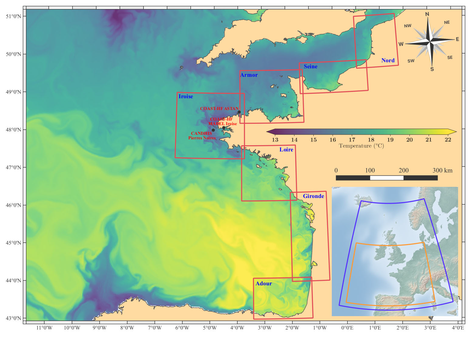
Figure 5 A Bay of Biscay configuration with seven magnified views at 500 m resolution (red rectangles). The 2.5 km resolution coarser grid (orange rectangle) is included in a larger 2D model at 5 km resolution (blue rectangle). The sea surface temperature is given for 16 August 2018 with the finest possible resolution. Bathymetric and coastline sources: Ifremer, Service hydrographique et océanographique de la marine (SHOM) and Natural Earth.

2.4 Computational cost

To evaluate the performance of this implementation, several tests were performed with the regional and coastal configurations, presented in the following sections, with classical offline one-way nesting and two-way nesting. First, the coarser model was run independently over the whole computation period to obtain information to force the child grid area at an hourly frequency. Second, baroclinic currents, temperature and salinity variables were interpolated horizontally and vertically onto the child grid with an external homemade Fortran tool. For the regional configuration usually composed of seven child grids, only the one focused on the Iroise Sea (see Fig. 5) was kept for this experiment.

Table 1 summarizes the computational times for MARS3D one-way classical offline nesting and MARS3D-AGRIF two-way nesting. For this experiment, the time integration lasts 45 d. All the simulations were performed on the Datarmor supercomputer, which is composed of 396 nodes with 28 cores each (https://www.ifremer.fr/fr/infrastructures-de-recherche/le-supercalculateur-datarmor, last access: 15 February 2023). Since the computing performance depends on the load of the machine, the computational cost was evaluated from a pool of repeated experiments (five times). For each configuration, the different models (one-way and two-way) were run with the same MPI rank distribution but from two different parallelization methods, namely the classic MPI domain decomposition and the hybrid computation (MPI and OMP) mode.

Table 1 Mean computation time given in hours for both modeled configurations for a simulation of 45 d.

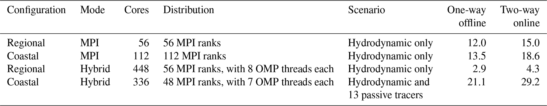
For both configurations, the computation time is increased by one-third for the AGRIF configuration compared to the classical offline one-way nesting. This difference is explained by two extra steps performed by the AGRIF library, i.e., the spatial interpolation to prepare the fine-grid boundary conditions and the update process from the fine grid to the coarse one. It is worth noticing that the handling time of the 3D output files and the waiting time due to the activity on Datarmor were not included in the one-way nesting duration. Their introduction would decrease the difference, especially if several magnifications are implemented.

As shown with the regional example, using hybrid parallelization with 8 times more computational resources than with MPI decreases the decreases the total time by 4 times. The hybrid mode is an efficient way to require more resources without considering the domain decomposition in complex geographic areas. Finally, the advection–diffusion evolution of 13 passive tracers in the coastal configuration is another example in which the hybrid mode makes it possible to achieve reasonable calculation times.

3 Systematic refinement of the coastal zone: paving the French Atlantic coast within a regional configuration

3.1 Bay of Biscay configuration

The MARS3D model has already been used to investigate the Bay of Biscay and its extension to the western English Channel (Huret et al., 2013; Lazure et al., 2009). Here, the MARS3D-AGRIF capability is implemented along the northwestern European continental shelf. Figure 5 shows how the AGRIF skill is used to pave the coastline from Spain to Belgium with overlapping grids. Seven 500 m resolution magnifications of approximately the same grid size are embedded into a coarser 2.5 km resolution grid. A total of 40 generalized σ layers discretize the vertical axis with a stretching function that induces refinement above 150 m depth next to the surface. Even though the space-refinement factor is 5, the time refinement is adapted according to the maximum velocity encountered within each grid. It is either a factor of 3 (over areas with relatively slow flows) or 5 (in very energetic areas such as the middle of the English Channel). Similarly, the turbulent viscosity coefficient (Laplacian operator) differs between each magnification and ranges from 0.5 up to 3 m² s⁻¹. At the surface, Météo-France atmospheric forcings drive the dynamics, with an ARPEGE (Action de Recherche Petite Echelle Grande Echelle) high-resolution (0.1^∘; hourly) analysis for the coarser grid and AROME (Application of Research to Operations at Mesoscale; 2.5 km; hourly) analysis or the child grids. The main hydrological runoffs are set in the magnifications (96 rivers). They come from different source databases (Spanish, English, French and Dutch). At the open boundaries of the coarse grid, daily temperature and salinity conditions are provided by the Mercator PSY2V4 re-analysis. The tidal signal is issued from a larger 2D model (5 km resolution) forced by the FES2014 (finite element solution) ocean tide atlas with 14 harmonic constituents (Lyard et al., 2021). The sea level is imposed, while a zero gradient condition is applied to normal and tangential currents.

A realistic two-way hindcast has been realized over the period 2010–2019. To demonstrate and characterize AGRIF nesting benefits, a one-way configuration has been run on the Iroise grid over the years 2017–2018 as a reference. These 2 common years have been selected from the available datasets for several validation parameters (detailed in Appendix A). A 3-month spin-up was performed for each hindcast. The forcing and parameterization of the offline one-way hindcast are those used in the two-way configuration, apart from the tidal sea level signal, which comes from the 112 harmonic components of the SHOM CST France model (le Roy and Simon, 2003). The temperature and salinity open-boundary conditions come from the above mother grid integrated without child grids. This tidal model has been accurately validated throughout the French tidal gauge network of RONIM.

3.2 Hydrodynamic impact over open boundary conditions

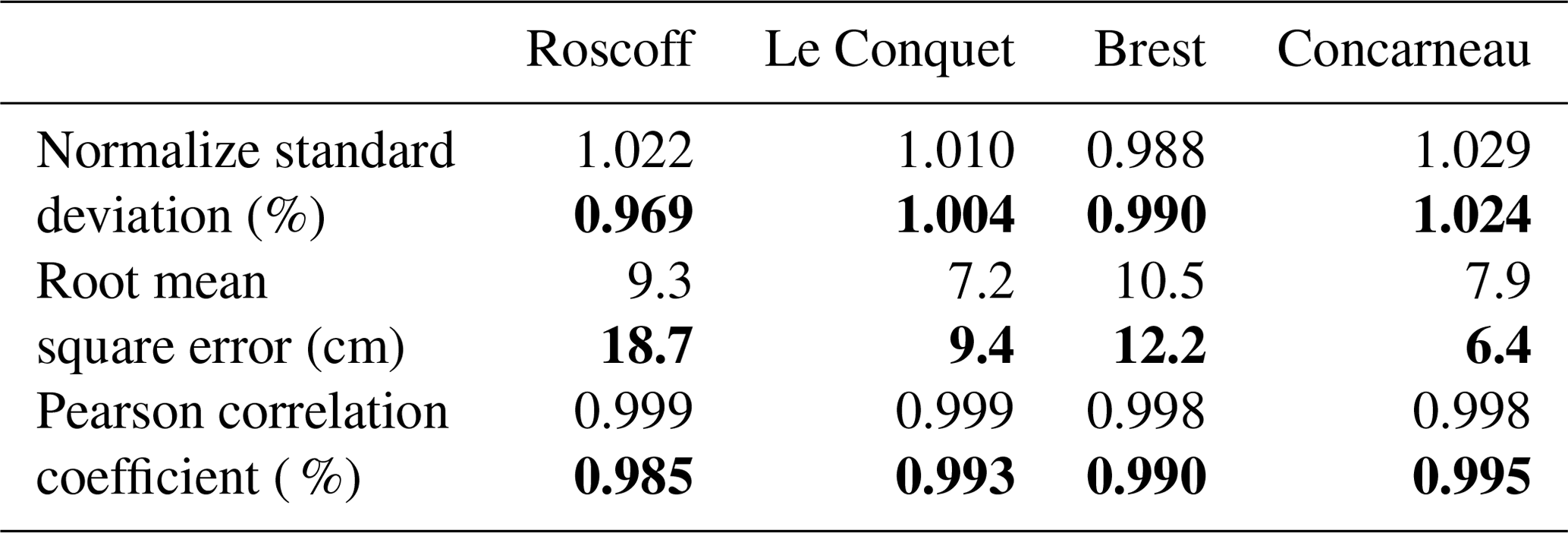
The tidal signal (extracted from the Iroise 500 m grid) is compared to hourly validated data of four tidal gauges available in the studied area. The main statistics are estimated over 1 year and given in Table 2. The tide modeled with the two-way technique is slightly less precise than with the one-way simulation. It is especially true at the northeastern boundary, at Roscoff, where the RMSE is twice as large. On the opposite side, at the southern boundary, at Concarneau, the differences are in favor of the two-way nesting.

Table 2 Comparison of the sea surface elevation between the MARS3D one-way (roman font) and MARS3D-AGRIF two-way (bold font) for the Iroise magnification (500 m horizontal resolution), compared to the RONIM tidal gauges.

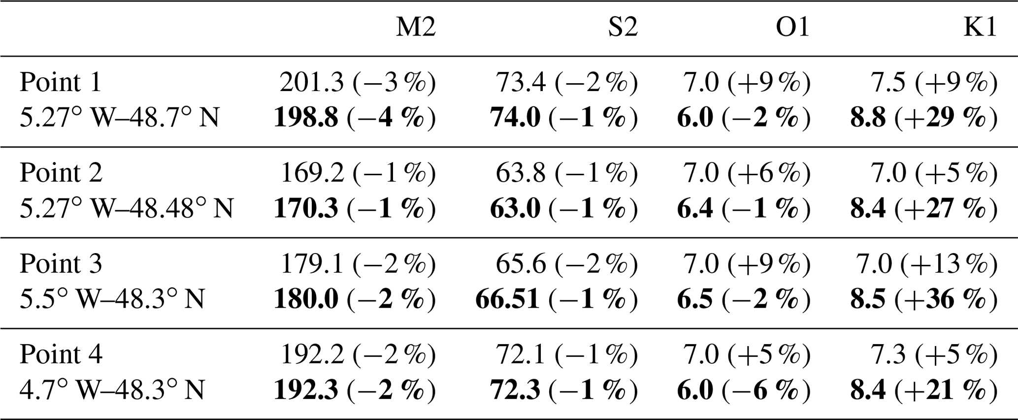
To observe the influence of the tide propagation, the signal modeled by Iroise magnification is compared to the PREVIMER harmonic component atlas. This atlas was built upon a series of barotropic simulations at 250 m horizontal resolution and validated with the RONIM network (Pineau-Guillou, 2013). A harmonic decomposition was applied to each hourly time series extracted from the hindcasts covering an entire year. Table 3 compares the wave elevations for the waves M2, S2, O1 and K1 at four locations in the Iroise Sea. Both models are in fairly good agreement with the reference atlas. The main difference is found for the wave K1 and MARS3D-AGRIF two-way configuration. The wave K1 is over-estimated by 20 % for the relative difference, but the amplitude itself differs by less than 2 cm.

Table 3 Comparison of the wave elevation amplitudes between MARS3D one-way (roman font) and MARS3D-AGRIF two-way (bold font) for the Iroise magnification (500 m horizontal resolution). The model amplitudes are given in centimeters, with the relative difference between model and observation given in percent.

A similar comparison has also been done for the barotropic currents. The differences are higher for the minor waves of O1 and K1. They reach up to 5 cm s⁻¹ and 30 % in relative difference at some locations (not shown). However, the validation of the PREVIMER atlas currents was not available all over the area, due to a lack of long time series data for the French coast. Barotropic currents have therefore been compared to different available Acoustic Doppler Current Profile (ADCP) datasets recorded in the bay of Brest or Molène archipelago over shallow waters. No significant difference has been found between nesting techniques.

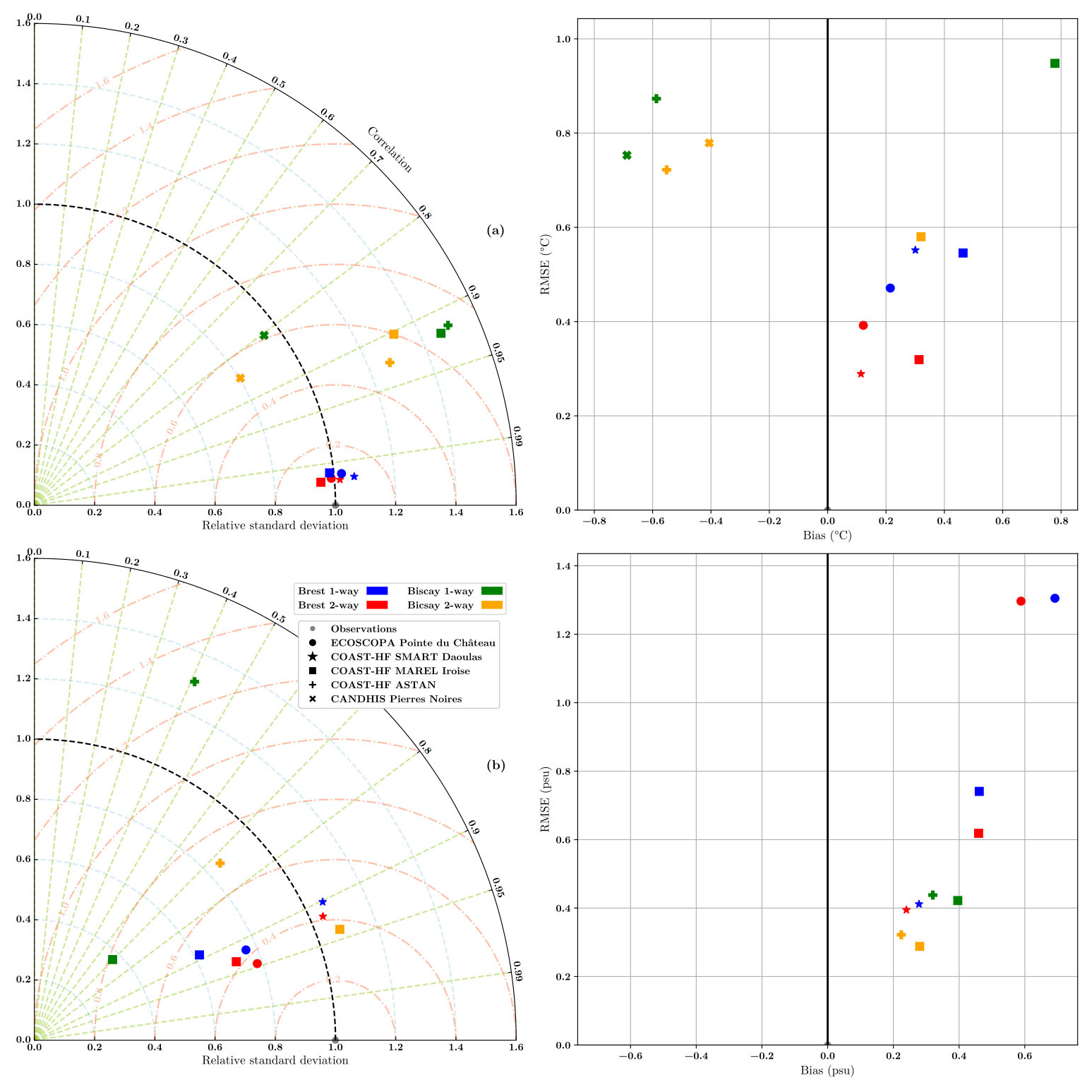
Figure 6 Temperature (a) and salinity (b) validation for both configurations. The Taylor diagrams are represented with the relative standard deviation (dashed blue lines), correlation (dashed green lines) and relative root mean square error (dashed red lines).

3.3 Hydrologic validation

A detailed qualification of the regional Bay of Biscay configuration has been done by Bezaud and Pineau-Guillou (2015). It highlighted the enhancements in predictions with increasing resolution in the coastal areas where the 500 m magnification models have been implemented. These comparisons have been made against coarser models. As expected, the authors concluded that a finer resolution allows the model to simulate the small-scale structures (instabilities of the front, eddies, filaments, etc.) accurately.

Here, the two-way versus one-way nesting is evaluated over 2017–2018. The evaluation focuses on the Iroise Sea magnification with different mooring stations (see the black points in Figs. 5 and 8). Figure 6 displays Taylor diagrams for temperature and salinity. A third diagram represents the bias values and root mean squared errors (RMSEs). These graphs summarize the comparisons between the available datasets (see Appendix A) and both nesting methods.

The nesting impact is not homogenous all over the domain. First, the two-way nesting technique improves the model's overall performance compared to oceanic datasets (see the green points for one-way and yellow points for two-way configurations). The simulated temperature offsets are noticeably reduced. The primary favorable impact is the drop in the root mean square error by 0.4 ^∘C for the COAST-HF-MAREL-Iroise buoy (where COAST-HF is Coastal Ocean Observing System – High Frequency). For salinity comparisons, the RMSE and the bias are of the same order of magnitude. The significant improvement relies on the enhancement of correlation for the COAST-HF-ASTAN dataset. This could be due to the proximity of this point to the eastern border of the magnification. The update capability of AGRIF two-way enables more realistic incoming fluxes at a high temporal resolution. The relative standard deviation of the simulated salinity at the MAREL-Iroise buoy is also considerably reduced.

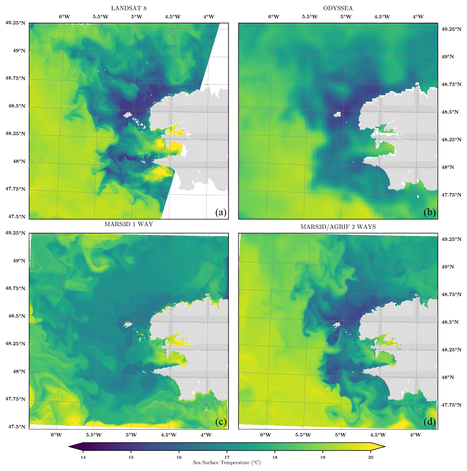
Figure 7 Sea surface temperature over the Iroise Sea on 15 August 2016 for Landsat 8 (a), ODYSSEA (b), a one-way simulation (c) and a two-way simulation (d). Coastline source: SHOM.

3.4 Focus on particular processes

In the Iroise Sea during the summer, the Ushant front is depicted by cold water of about 14 ^∘C. Over shallow depths, the tidal currents are intensified and very strong around Ushant and the Molène archipelago. The induced tidal stirring is so large that waters are mixed (and homogeneous) from the sea surface to the bottom. Further offshore, the summer stratification can develop, and the sea surface is warmer (above 18 ^∘C). This phenomenon can be seen from satellite data on 15 August 2016 (Fig. 7) for both Landsat 8 and ODYSSEA products (described in Appendix A). Compared to ODYSSEA, the Landsat surface temperature is overestimated in different spots near the coast, in the bay of Brest, for example, with values over 20 ^∘C which might be due to mis-flagged clouds.

The ability of the two-way nesting approach (Fig. 7d) to correctly reproduce this spatial feature is evident, while the one-way nesting (Fig. 7c) struggles to simulate this phenomenon. Indeed, the Ushant front is nearly missing in the one-way simulation. It is much better characterized in the two-way simulation at 5.25^∘ W, with more realistic temperature magnitudes on each side of the front, thanks to the AGRIF update. Furthermore, the realism of the sub-mesoscale structures around the shoals of Sein Island (Île de Sein) and in the Molène archipelago is improved. On the other hand, one can notice the open-boundary effect in the southern part of the one-way simulation, where an east–west temperature front is created. It is related to the upwind scheme applied to temperature and salinity open-boundary conditions (i.e., applying an external value when the water mass enters the domain).

For wide-open areas such as the Iroise Sea, the benefit of the feedback or update of the magnification not only contributes to the correct representation of the thermic Ushant front, mainly by enlarging the span of the scale captured (e.g., fine eddies and filaments), which is expected, but also in terms of the horizontal localization of thermal front, which is less expected. As a matter of fact, the forcing through the open boundaries is of primary importance for limited area models; it may dramatically impact the local coastal processes, even in areas where the dynamics are highly controlled by large scales such as the tidal forcing. Even though the tidal signal is better represented with the one-way nesting (due to the CST France model), the upwind scheme applied for tracers at open boundaries is not accurate enough for hourly heat exchanges. The chosen simulated domain is not large enough for one-way nesting to reproduce a sharp temperature front.

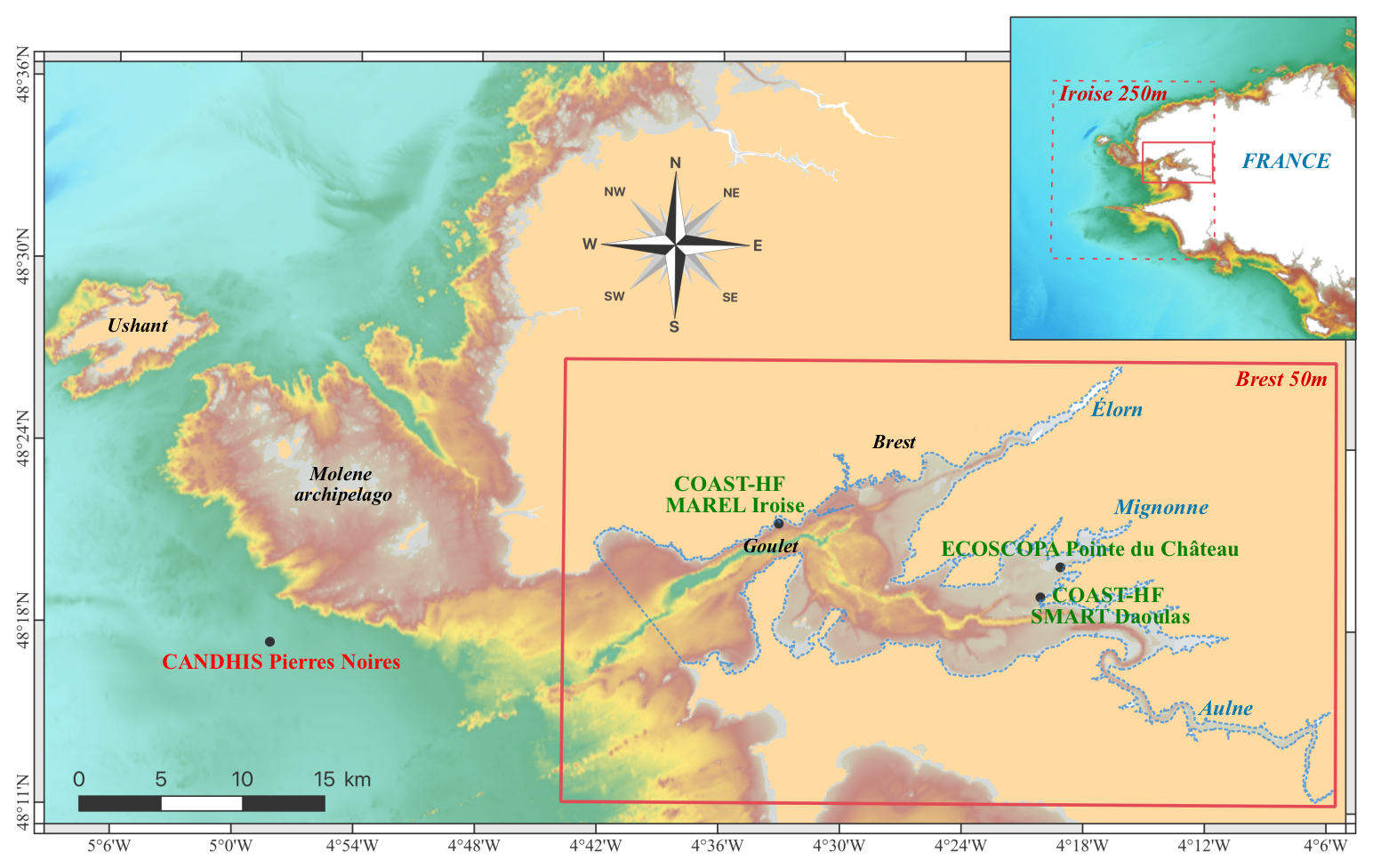
Figure 8 The bay of Brest configuration. The geographic extent of the magnified grid at 50 m resolution is the solid red rectangle. The coarser grid at 250 m resolution is the dashed red rectangle. The dashed blue line represents the control volume used for the estimation of the renewal indicator. Bathymetric and coastline sources: Ifremer SHOM.

4 Highlighting the benefit of a two-way conservative approach: estimating renewal time over a coastal area

4.1 Bay of Brest configuration

The bay of Brest is a semi-enclosed, macro-tidal ecosystem located at the western end of Brittany (France), covering more than 180 km². It is connected to the Iroise Sea through a 1.8 km wide by 6 km long and roughly 50 m deep inlet (called the Goulet de Brest). Due to its complex geometry and topography, the currents are strong, but relatively well known, and have been the focus of many previous studies. A dominant semi-diurnal tide characterizes this area, with a tidal range of 1.2 to 7.3 m. The tidal currents peak up to 3 m s⁻¹ in the Goulet and are in quadrature phase relative to the surface elevation (Petton et al., 2020). The mean volume at mid-tide inside the bay is roughly 2 × 10⁷ m³. As its average depth is only 8 m, the back-and-forth flow for each tide prevents stratification nearly everywhere (Le Pape and Menesguen, 1997). The tidal prism is 25 % of the mean volume in neap tide and 60 % in spring tide. Freshwater runoffs, mainly coming from the Aulne river, modify the hydrology locally (Auffret, 1983).

The MARS3D-AGRIF model has been set up over the Iroise Sea (47.74–48.82^∘ N; 4.08–5.55^∘ W) with a horizontal grid resolution of 250 m. As shown in Fig. 8, a magnification over the bay of Brest (48.20–48.44^∘ N; 4.09–4.72^∘ W) is introduced, with a resolution of 50 m. The time and space refinement factors are both equal to 5. The vertical discretization is performed with 20 equidistant σ layers in both grids. The bathymetries have been interpolated from a combination of digital terrain models (SHOM, Ifremer, and IGN, the French National Institute of Geography and Forestry). This Iroise model is forced by harmonic components from the SHOM CST France atlas (le Roy and Simon, 2003). The 3D open-boundary conditions for baroclinic currents, temperature and salinity are imposed at an hourly frequency from a hindcast of the previous regional configuration (Caillaud et al., 2016). Freshwater inputs for the four main rivers in the bay have been taken from the French HYDRO database (http://www.hydro.eaufrance.fr/, last access: 15 February 2023) and corrected with corresponding watershed surface rates. The atmospheric forcings rely on the Météo-France AROME (2.5 km; hourly) analysis. The configuration is available from Petton and Dumas (2022a), along with a detailed description of the physical and numerical parameterizations.

4.2 Hydrologic validation

Two realistic hindcasts have been run from 2017 to 2019 for both one-way and two-way nesting techniques. Previous studies have already validated the coastal bay of Brest one-way configuration in detail (Petton et al., 2020; Frère et al., 2017). In fact, the large-scale features of the macro-tidal flow are easily captured (Petton et al., 2020) in such a semi-enclosed area. And, due to high turbulent mixing in the area, the dynamics are less sensitive to boundary effects. Consequently, the two-way nesting technique barely enhances the results. The tidal features are the same (not shown), while the hydrology is slightly modified (blue and red points for one-way and two-way nesting, respectively, in Fig. 6). Indeed, the two-way nesting reduces the bias in temperature. The feedback, which enables a more accurate global temperature budget in the mother grid, could explain this improvement. Moreover, the two-way technique reduces the relative standard deviation in salinity for the MAREL-Iroise and ECOSCOPA datasets. As the water runoffs are identical, this amelioration might be hard to explain. Nevertheless, it may result in a better simulation of current flows, according to nonlinear effects.

4.3 Timescale indicator

As the shallow ocean is subject to considerable environmental and anthropogenic pressures, the fate of coastal waters is a key to environmental, ecological and economic issues. Therefore, global and local indicators are crucial for stakeholders to anticipate the spread of different materials such as oil (Jordi et al., 2006), micro-plastics (Frère et al., 2017), biogeochemical processes due to nutrients release (Le Pape and Menesguen, 1997; Fiandrino et al., 2017) and pollution phenomena (Jiang et al., 2017; Neal, 1966) and to develop restoration solutions (Kininmonth et al., 2010; Rossi et al., 2014; Thomas et al., 2014).

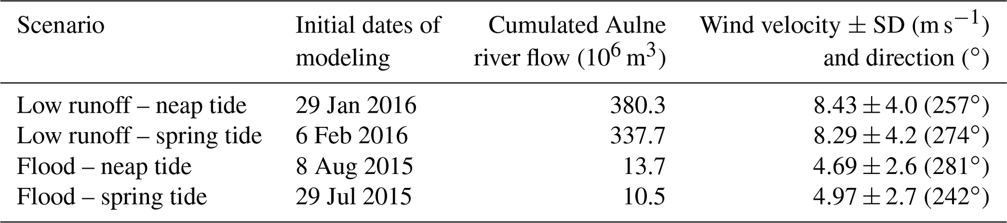
Table 4 Environmental condition for the mean of each computation period over the first 30 d of the simulation. Note that SD is the standard deviation.

4.3.1 e-folding flushing time estimate

In this study, the water renewal time in the bay of Brest is evaluated from the flushing time indicator. This diagnostic gives the time for 67 % $(\mathrm{1}-\mathrm{1}/e)$ of the water in a control volume to be renewed. As the incoming flow may take some time to reach (parts of) the control volume, the flushing lag t₀ represents the time required for 5 % of the water mass to be flushed out by the inflow. It allows understanding where the inflow comes from. Consequently, the e-folding flushing time θ is, more precisely, the decay time in the concentration from 95 % down to $\mathrm{1}/e$ of initial concentration using an exponential regression $C\left(t-t_{\mathrm{0}}\right)=e^{-\left(t-t_{\mathrm{0}}\right)/\mathit{\theta }}$ (Jouon et al., 2006; Grifoll et al., 2013; Plus et al., 2009). The e-folding flushing time is estimated locally to provide spatially distributed information on the water-renewal capacity of a basin or over the entire control volume. Then, the global flushing time is the average of the local flushing times.

In the bay of Brest, the water inflow can come from the rivers or tidal progression. To identify the relative importance of these two processes, the volume control has to extend over the entire bay plus the outer part of the bay in which only the tide is at play (see the dashed blue line in Fig. 8). For an accurate estimate of the e-folding flushing time, the simulated domain has to be larger than the control volume (Viero and Defina, 2016). Indeed, the return flow through the Goulet due to the semi-diurnal tide is likely to influence the water mass displacement and, therefore, the renewal time. Thus, the two-way nesting is expected to be an adequate tool; after crossing the open boundary, a particle can re-enter the simulated domain in the full nesting, while it is lost in the one-way method.

In our experiment, the flushing time is estimated on an Eulerian reference system by simulating the dilution of passive tracers whose initial concentration is set to 1 inside the control volume (in the fine grid) and 0 everywhere else. Water coming from the ocean (outside the Iroise Sea) and river runoff has a tracer concentration equal to 0. The outflow concentrations are lost when crossing the model grid (mother grid in two-way nesting). To remove of the initial tide conditions, the release of tracers is repeated 13 times every hour for an even coverage of the tidal cycle (Plus et al., 2009). The final indicator is the average of the 13 estimations.

4.3.2 Case scenario

Various numerical experiments have been performed to catch variable conditions and estimate an exhaustive renewal indicator. Each simulation has been carried out according to the same protocol, with a hydrodynamic spin-up run performed over 1 month before the release of passive tracers. To obtain various tidal regimes and hydrologic runoffs, the study focuses on four scenarios related to the tidal range and runoffs, where releases have been done at the beginning of spring tides and neap tides, in winter and summer seasons, during flood and weak runoff events. All of these simulations have been performed with realistic atmospheric forcings, even though the wind direction and intensity are highly variable at mid-latitudes. First, it is challenging to find 15 d wind sequences that characterize the local atmospheric forcings. Second, the bay has a macro-tidal regime, so the water is mixed, whatever the weather conditions. We then focus on the two dominant runoff regimes (flood water vs. low runoff) combined with the initial phase of the tide (spring vs. neap tides), as detailed in Table 4.

4.4 Flushing times of the bay of Brest

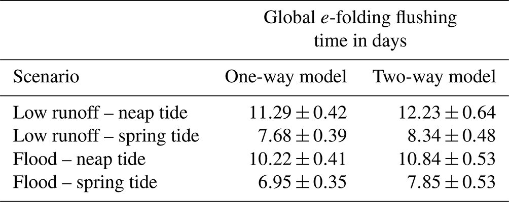
The issue addressed here is the evaluation of the capability of the MARS3D-AGRIF tool to characterize the renewal capacity of the bay and identify the role played by the tidal forcing and river runoffs. The indicators have been estimated with both nesting methods for the four scenarios. The flushing times of the whole control volume are given in Table 5. As expected, low river runoffs imply a longer renewal time than flood situations. However, the initial tidal phase is the main change factor between the scenarios, with more intensive mixing during spring tides. There is a positive offset (roughly 10 %) of the renewal time from AGRIF two-way simulations. This shift is due to the return flow within the bay during each tidal cycle, which is underestimated in the one-way model, as its boundaries act as a sink for the tracer.

Table 5 Global e-folding flushing times and standard deviation in days for the whole control volume for both modeled configurations. The deviation is estimated over the 13 time-released simulations for each scenario.

The local e-folding flushing times estimated with the two-way nesting configurations are displayed in Fig. 9 for the four scenarios. The indicator increases as the geographic position moves away from the control volume boundary. In contrast to the global indicator, the runoff impact on the renewal capacity of the bay is obvious. In low river runoff conditions, the southeastern part of the bay is isolated from the rest. The local e-folding flushing time reaches more than 25 d in shallow coves and is released at neap tide. The impact of tide is the next level in order of importance, with, not surprisingly, stronger renewal during spring tide than neap tide. In each scenario, the central energetic eddy stands out because it is the rallying point of continental waters.

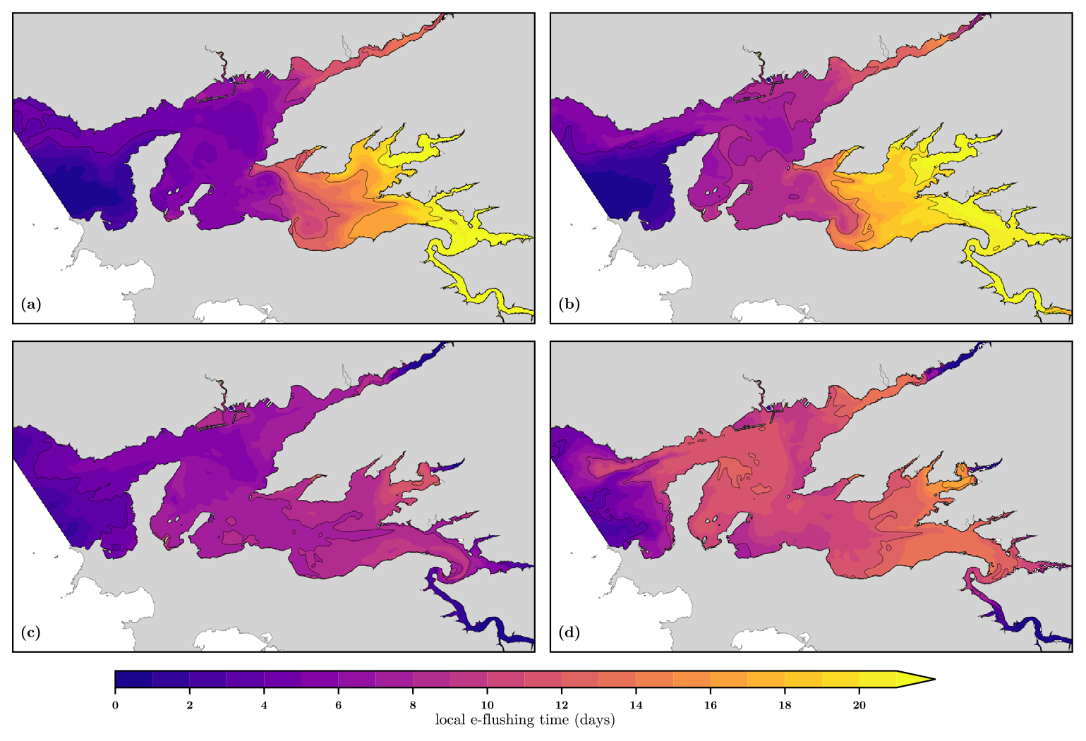
Figure 9 Local e-folding flushing time estimated for spring (a) and neap (b) tides in low-flow conditions and for spring (c) and neap (d) tides for flood conditions. Coastline source: SHOM.

Figure 10 Differences between local e-folding flushing times estimated with one-way configuration over the two-way nesting method. They are computed for spring (a) and neap (b) tides in low-flow conditions and for spring (c) and neap (d) tides for flood conditions. Coastline source: SHOM.

The relative differences in local e-folding flushing time estimates are illustrated in Fig. 10. Whatever the environmental conditions, the one-way nesting overestimates the renewal capacity of the bay by predicting lower local e-folding flushing times nearly everywhere. Such bias is expected because the one-way nesting does not correctly follow the tidal prism in the control volume: any tracers that leave the volume are lost for the estimate of the e-folding flushing time. In the inner part of the bay, the local differences are always negative and reach around 20 % in flood conditions. Under low river runoff conditions, the renewal time is independent of the tide regime in the central part. In this area, the water mass is always replaced by the inflow during the period of simulation, so the treatment at the open boundary does not matter. In contrast, e-folding flushing time estimates are underestimated in shallow areas, especially during spring tides. To ensure that the disparities are due to open-boundary treatment, a similar experiment was run with a much smaller control volume located only within the bay. Then, the simulated domain is larger than the control volume, and the results are identical, regardless of the nesting method. This highlights the asset of the two-nesting approach for the evaluation of the water renewal times. Last, some suspicious patches appear at the western part of the control volume, which only takes into account tidal inputs. Others are visible next to the river mouths. Both are related to the initial time release and inaccurate exponential regression, as the inflow quickly replaces the initial water masses (as confirmed by de Brauwere et al., 2011).

5 Discussion

The first objective of grid refinement is either to tackle a local stationary problem or to follow a single dynamical structure along with its displacements (Blayo and Debreu, 1999). In the MARS3D structured grid model, the magnification allows us to reach a resolution commensurable with the Rossby internal radius or with the coastal geometry in the presence of islands, capes or peninsulas. Unfortunately, the use of the ADI algorithm in MARS3D makes the implementation of the two-way AGRIF nesting tricky. In addition, coastal applications require the management of wetting–drying. Still, the present applications demonstrate the capabilities of MARS3D-AGRIF two-way nesting to represent the macro-tidal dynamics and propagate the tracers in coastal areas. They also illustrate how it improves the monitoring of the fate of coastal water.

Despite the regular improvement in the computational power available for high-performance scientific computing, the computational cost and the storage of massive datasets remain significant issues for long-term numerical oceanic simulations due to various reasons, such as green computing considerations. We hereafter review the different key advantages provided by the introduction of the AGRIF library in MARS3D.

Regarding parameterization, the AGRIF library allows the specification of different forcings (meteorology and runoff) or numerical schemes for each grid of the hierarchy. Consequently, the parameterizations can fit every local process. In addition, the local time refinement is specific to each grid (ratio of 3 to 5). The more intense the dynamics, the more the time refinement factor is increased.

The AGRIF flexibility also lies in the way child grids of a given hierarchy can either be added or easily removed. An offline bathymetric update tool, available with MARS3D code, modifies both mother and child bathymetries to fit fluxes (from one grid to another) along child borders. Once the bathymetry consistency is performed, users can launch the runs without additional tasks. The initial conditions for the new magnification are estimated online by the AGRIF library. This capability has been used to study the deep convection in the northwestern Mediterranean Sea more precisely (Garreau and Garnier, 2015) or to better identify the shear stress on marine renewable energy structures (Christophe Maisondieu, personal communication, 2019). If a user needs to remove a specific child grid, then the bathymetry of the mother grid simply has to be recomputed with the tool before launching the model.

The usual offline nesting procedure requires writing and storing of 3D forcing files from which the open-boundary and initial conditions for the child grid are supplied. To prevent aliasing or spurious incompatibilities between barotropic and baroclinic modes, high-frequency outputs must be saved to a hard drive. In every instance in which tidal dynamics are dominant, a massive amount of input–output (I/O) is involved, which raises other kinds of issues, such as how to write massive data in a massive parallel context. Despite the many improvements to deal with this issue, like exporting the I/O on dedicated central processing units (CPUs) with the XIOS library (Yepes-Arbós et al., 2022), the cost of long-term storage of massive data cannot be escaped. The on-the-fly grid nesting procedure (encompassing initial and open-boundary management) included in the two-way nesting circumvents these tedious steps by performing them online at each time step and for the different grids of the hierarchy.

Another point concerns the vertical coordinate framework, which is here a sigma one in MARS3D. The vertical interpolation towards a sigma framework often requires projection onto a geopotential framework to perform a split horizontal–vertical interpolation. Such split interpolations on temperature and salinity fields can lead to gravity instabilities in the case of significant bathymetric inconsistencies between the coarse and child grids. Therefore, the user must carefully define the interpolation parameters (such as those defining the intermediate geopotential framework onto which the vertical interpolation is performed) and check the consistency of the gravity gradient. As MARS3D-AGRIF two-way nesting requires a perfect fit of the vertical discretization for all grids of the hierarchy and bathymetries coherence, these constraints prevent the gravity issues. Of course, this well-known problem may also be avoided in offline embedding procedures by taking the same care in defining the grid and the bathymetry computations.

The traditional one-way nesting remains a lighter solution than the AGRIF two-way nesting, especially in case repeated experiments are required for tuning purposes, with different parameterizations, or for exploring several environmental hypotheses (Cadier et al., 2017; Petton et al., 2020; Gangnery et al., 2019). As open-boundary files can be reused at no cost, this method is still a good approach to improving numerical developments in coastal models. However, the two-way update process is compulsory when the final objective is to ensure a conservative approach (biological tracer, connectivity study, etc.) over large geographic areas at minimum cost. It is not a unique solution as for other kinds of spatial discretization, such as unstructured, curvilinear or polar-style coordinates, but meets the same numerical constraints. The two-way nesting proposed here keeps it simple for the end-user.

As shown in Sect. 3.2, the online interpolation from the mother to child grid and the update process preserve the propagation of tidal elevations and currents with an equivalent level of accuracy to the one achieved with the SHOM CST France tidal forcing prescribed at the open-boundary conditions of a single typical coastal grid (some tens of kilometers of extension, with 10 to 100 m depth, at a resolution of some hundreds of meters). The observed differences between the two-way nesting and the one-way offline methods are less than a few centimeters, which are not significant in coastal areas. It is thus a real performance, first, because, in the two-way nesting approach depicted here, the tidal propagation computed at the coarse-grid level is fed with a FES global reference tidal solution (Lyard et al., 2021) far away from the coasts. And, second, because the use of the ADI algorithm requires that the coarse solution be updated over the entire child domains from the spatial average of their fine solutions. Therefore, it proves that the MARS3D-AGRIF implementation conserves mass and momentum and that the interactions between the child grids are handled accurately over open sea and over wetting–drying areas. In conclusion, MARS3D-AGRIF represents tides at regional and coastal scales and at medium resolution (Lazure et al., 2009; Muller et al., 2014). It is well suited for large configurations with several magnification models and for long-term hindcast or operational forecast simulations to monitor the marine environment.

Regarding environmental applications, Sect. 4.3 confirms that the two-way nesting solution is mandatory to accurately estimate indicators characterizing the mixing within a bay, especially in macro-tidal regimes. For estimates defined over a control volume, the management of the open boundaries is a key element. On a stand-alone grid, when the flow enters the domain, users can either choose to apply or nudge towards a constant value (zero or whatever value), a time series inferred from a large-scale solution (if available) or a zero-gradient condition. In all cases, the solution is strongly non-conservative, resulting in discrepancies in the final indicators. Even the one-way nesting is not conservative when the control volume is too close to an open boundary. Beyond the estimation of coastal indicators, the MARS3D-AGRIF two-way capability improves the management of the fate of a tracer outside the bay at the coarser horizontal resolution (and at a fairly reasonable computational cost). It also enforces accurate incoming concentration across the open boundaries of the child grids. Such a conservative approach is relevant for applications with sediment, biological or chemical dynamics models.

Finally, it is worth noticing that such a software can also perform the opposite, i.e., grid coarsening. It is a relevant capability for online physical–biogeochemical coupling. Such an approach has been used by Lévy et al. (2012) in an offline mode. Capturing relevant scales of the oceanic flows may require a higher spatial resolution than that required by the main biogeochemical features. For instance, the sub-mesoscale features enhance the vertical exchange and refuel the surface with nutrients. A few hundred meters of spatial resolution is mandatory to simulate sub-mesoscale dynamics. But it is unaffordable for state-of-the-art biogeochemical models that use and advect tens of tracer fields (Heinze and Gehlen, 2013). The AGRIF coarsening capability allows this differential resolution (physics at high resolution and biogeochemistry at lower resolution) by building online non-divergent transport fields from the high-resolution grid onto the coarse-resolution grid. In that way, the “grandmother” grid may completely overlap the mother grid.

Appendix A: Data used for validation

The tidal validation is based on four stations from the French tidal gauge network RONIM, which is maintained by SHOM. Moreover, three datasets are available in the framework of the national program COAST-HF (Coastal Ocean Observing System – High Frequency; https://www.coast-hf.fr, last access: 15 February 2023), which gathers 14 automated moored buoys. The COAST-HF ASTAN buoy (48.749^∘ N; 3.961^∘ W) is a cardinal buoy of opportunity located 3.1 km offshore from Roscoff, east of Île de Batz (Isle of Batz). It has recorded data every 30 min at 5 m depth since 2008 (Gac et al., 2020), over a mean bathymetry of 45 m. The COAST-HF-MAREL-Iroise buoy (48.357^∘ N, 4.582^∘ W) is located at the entrance of the bay of Brest and has recorded data every 20 min at 2 m depth since 2000 (Rimmelin-Maury et al., 2020). Inside the bay of Brest, next to the Mignonne river mouth, the COAST-HF-SMART-Daoulas buoy (48.317^∘ N, 4.331^∘ W) has been monitoring parameters at 50 cm over the seabed at 15 min frequency since 2016 (Petton et al., 2021b). Next to this last point, the Ifremer observatory network, ECOSCOPA, has a study site called Pointe du Château (48.335^∘ N, 4.319^∘ W), which is at an oyster farm in the intertidal zone. Temperature and salinity data have been available at a 15 min frequency since 2008 (Petton et al., 2021a). We also had access to the sea surface temperature data from the Datawell buoy of Les Pierres Noires, which is part of the swell monitoring network CANDHIS (CEREMA; https://candhis.cerema.fr/, last access: 15 February 2023) and located in the middle of the Iroise Sea (48.29^∘ N, 4.97^∘ W). These monitoring stations are presented in Figs. 5 and 8.

Besides, satellite data are used for sea surface temperature (SST) validation at two different horizontal scales. The first one is based on SST fields extracted from the global Advanced Very High Resolution Radiometer (AVHRR) Pathfinder v5 daily dataset. The ODYSSEA chain has been modified by Saulquin and Gohin (2010) to use an optimal interpolation for the reconstruction of gap-free data, and it uses the previous analysis as a first guess. The product is gridded at a 0.02^∘ spatial resolution and is freely available at https://resources.marine.copernicus.eu (last access: 15 February 2023; Autret and Piolleì, 2018). The second one is based on the Thermal Infrared Sensor (TIRS) from the Landsat 8 satellite. As it orbits the Earth in a sun-synchronous, near-polar orbit inclined at 98.2^∘, one has a track over our area of interest every 8 d. Consequently, it is hard to extract snapshots without too many clouds. Recently, the United States Geological Survey (USGS) has started to distribute Landsat Collection 2 Level-2 (values are given after atmospheric corrections) with a calibrated land surface temperature field. The development of a water temperature algorithm is not the aim of this paper and represents a challenge by itself (Vanhellemont, 2020). However, the use of such a high-resolution product (30 m gridded) is very useful to detect fine structures. In that respect, the ODYSSEA product is complementary to the Landsat 8 scene and a reference on a coarser grid. To discriminate water temperature from clouds or land values, the quality index given for each pixel for this collection is used.