An ensemble Kalman filter-based ocean data assimilation system improved by adaptive observation error inflation (AOEI)

A previous study proposed an adaptive observation error inflation (AOEI) method for an ensemble Kalman filter (EnKF)-based atmospheric data assimilation system to assimilate all-sky infrared brightness temperatures. Brightness temperature differences between clear- and cloudy-sky radiances are large, and observation-minus-forecast differences (or innovations) are therefore likely to be large around boundaries between clear- and cloudy-sky regions. The AOEI method mitigates these discrepancies by adaptively inflating observation errors. Ocean frontal regions have similar characteristics to the borders between clear- and cloudy-sky regions with large innovations. Consequently, we have implemented the AOEI with an EnKF-based regional ocean data assimilation system, in which the assimilation interval is set to 1 d to utilize frequent satellite observations. We conducted sensitivity experiments to investigate the impacts of the AOEI on salinity structure, geostrophic balance, and accuracy. A control run, in which the AOEI is not applied, shows the degradation of low-salinity North Pacific Intermediate Water around the Kuroshio Extension region, where the innovation amplitude and forecast ensemble spread are large in association with the fronts and eddies. The resulting large temperature and salinity increments weaken the density stratification, leading to large vertical diffusivity. As a result, the low-salinity water in the intermediate layer is lost through strong vertical diffusion. When the AOEI is used, the salinity structure in the ocean interior is preserved because the AOEI suppresses the salinity degradation by reducing the temperature and salinity increments. We also demonstrate that the AOEI provides significant improvement of the geostrophic balance and the analysis accuracy of temperature, salinity, and surface-flow fields.

1 Introduction

The ensemble Kalman filter (EnKF) estimates flow-dependent forecast errors from an ensemble of model forecasts and calculates the best estimates (i.e., analyses) by combining forecasts and observations with their error covariances (Evensen, 1994, 2003). The EnKF has the advantage of being easy to implement for various models (see Table 1 of Ohishi et al., 2022), but it has been used in only two ocean reanalysis datasets thus far (Balmaseda et al., 2015; Martin et al., 2015): the Predictive Ocean Atmosphere Model for Australia (PAOMA) Ensemble Ocean Data Assimilation System (PEODAS; Yin et al., 2011) and TOPAZ4 (Sakov et al., 2012). In contrast, the three-dimensional variational method (3D-Var) is the most widely used in ocean analysis datasets (e.g., Miyazawa et al., 2017; Zuo et al., 2019).

With the enhancement of in situ and satellite observations, the number of observations has increased dramatically. Argo profiling float observations since the 2000s provide a large number of in situ temperature and salinity data in the ocean interior. Although satellite sea surface salinity (SSS) data since 2010 are relatively inaccurate, particularly in coastal and high-latitude regions (Abe and Ebuchi, 2014), previous studies have demonstrated the positive effects of SSS assimilation on the analyses of ocean interior structure such as mixed and barrier layers (Chakraborty et al., 2015), low-salinity water caused by river discharge (Toyoda et al., 2015), and El Niño–Southern Oscillation prediction (Hackert et al., 2011). A Japanese geostationary satellite, Himawari-8 (Bessho et al., 2016; Kurihara et al., 2016), has observed sea surface temperatures (SSTs) in the Pacific region at high spatiotemporal resolutions of 2 km and 10 min since July 2015. The Surface Water and Ocean Topography (SWOT) satellite is scheduled to be launched in 2022 and will provide high-resolution and two-dimensional sea surface height (SSH) anomalies (SSHAs).

For effective use of dense and frequent satellite observations, Ohishi et al. (2022) performed sensitivity experiments using an EnKF-based ocean data assimilation system with an assimilation interval of 1 d, which is more frequent than the 5 d and 7 d intervals in the existing EnKF-based systems (PEODAS and TOPAZ4, respectively). They demonstrated that the combination of incremental analysis update (IAU; Bloom et al., 1996) and relaxation-to-prior perturbation (RTPP; Kotsuki et al., 2017; Zhang et al., 2004) to restore the forecast ensemble perturbations toward the analysis by 80 %–90 % produced optimal results in terms of both dynamic balance and accuracy. However, their system contained several tuning parameters such as observation errors, ensemble size, and localization scale. Previous studies have prescribed observation errors in various ways, such as using spatiotemporally fixed constants (Miyazawa et al., 2012; Xu and Oey, 2014), assuming observation errors to be standard deviations calculated from historical observations (Miyazawa et al., 2009; Usui et al., 2006), estimating observation errors from other assimilation datasets (Penny et al., 2013), and assuming that observation error covariance matrices are proportional to the forecast error covariance matrices (Carton et al., 2018; Yin et al., 2011). A technique to adaptively inflate the observation errors based on the innovation statistics (Desroziers et al., 2005), which is called as an adaptive observation error inflation (AOEI) method, was recently proposed for assimilating all-sky infrared satellite brightness temperatures in an atmospheric data assimilation system (Minamide and Zhang, 2017; Zhang et al., 2016). As the brightness temperature differences between clear- and cloudy-sky radiances are large, there are large observation-minus-forecast differences (or innovations) around the boundaries between clear- and cloudy-sky regions, even for the tiny boundary differences between forecasts and observations. This results in erroneous analysis increments and degrades the analysis. AOEI mitigates the large discrepancies between forecasts and observations by adaptively inflating the observation errors. Ocean frontal regions such as the Kuroshio and Kuroshio Extension (KE) regions have large spatiotemporal variations, and the innovations around the frontal regions also tend to be large, even for small differences in frontal positions between the forecasts and observations. Therefore, ocean fronts have similar characteristics to the borders between clear- and cloudy-sky regions with large innovations, and the AOEI method is therefore expected to be useful for improving EnKF-based ocean data assimilation systems.

This study aims to investigate the causes of the salinity degradation around the KE region and to evaluate the impacts of the AOEI on the salinity structure, dynamical balance, and accuracy. The remainder of this paper is organized as follows: details of the AOEI method, the experimental design, the temperature and salinity budget equations, and the methods to evaluate geostrophic balance and accuracy in sensitivity experiments are presented in Sect. 2; Sect. 3 describes the causes of the salinity degradation in the intermediate layer and the positive impacts of the AOEI on the geostrophic balance and accuracy for temperature, salinity, and surface flow. A summary is provided in Sect. 4.

2 Methods

2.1 AOEI

Manual tuning of observation errors is computationally expensive, and several studies have proposed adaptive estimation methods using the innovation statistics of Desroziers et al. (2005):

$$\begin{array}{}\text{(1)}& \langle {\mathit{d}}_{\mathrm{b}}^{\mathrm{o}}({\mathit{d}}_{\mathrm{b}}^{\mathrm{o}}{)}^{\mathrm{T}}\rangle \approx {\mathbf{HP}}^{\mathrm{b}}{\mathbf{H}}^{\mathrm{T}}+\mathbf{R}.\end{array}$$

Here, 〈⋅〉 denotes the statistical expectation; ${\mathit{d}}_{\mathrm{b}}^{\mathrm{o}}(=\mathit{y}-\mathbf{H}\stackrel{\mathrm{‾}}{{\mathit{x}}^{\mathrm{b}}})$ is an innovation vector, where y, H, and $\stackrel{\mathrm{‾}}{{\mathit{x}}^{\mathrm{b}}}$ denote an observation vector, linear observation operator, and forecast ensemble mean state vector, respectively; and P^b and R are the forecast and observation error covariance matrices, respectively. Expressing Eq. (1) in a scalar form, the observation error σ_est-o may be estimated by

$$\begin{array}{}\text{(2)}& {\mathit{\sigma }}_{\text{est-o}}^{\mathrm{2}}=(d_{\mathrm{b}}^{\mathrm{o}}{)}^{\mathrm{2}}-{\mathit{\sigma }}_{H\left(x^{\mathrm{b}}\right)}^{\mathrm{2}},\end{array}$$

where ${\mathit{\sigma }}_{H\left(x^{\mathrm{b}}\right)}$ is the forecast ensemble spread in observation space. Here, the forecast ensemble spreads are assumed to be accurate, and $(d_{\mathrm{b}}^{\mathrm{o}}{)}^{\mathrm{2}}$ is assumed to be equivalent to $\langle (d_{\mathrm{b}}^{\mathrm{o}}{)}^{\mathrm{2}}\rangle$. To avoid underestimation of the observation errors, larger observation errors σ_o between the estimated and prescribed errors are used in the AOEI method (Minamide and Zhang, 2017; Zhang et al., 2016):

$$\begin{array}{}\text{(3)}& {\mathit{\sigma }}_{\mathrm{o}}^{\mathrm{2}}=max\left\{{\mathit{\sigma }}_{\text{pre-o}}^{\mathrm{2}},{\mathit{\sigma }}_{\text{est-o}}^{\mathrm{2}}\right\},\end{array}$$

where σ_pre-o is the prescribed observation error. As described in Sect. 1, the AOEI suppresses erroneous analysis increments associated with systematic errors, biases, and representation errors by adaptively inflating the observation errors when the squared innovation is larger than the sum of the prescribed observation and ensemble-based forecast error variances.

2.2 Experimental design

This study uses an EnKF-based regional ocean data assimilation system known as sbPOM-LETKF (Ohishi et al., 2022), comprising a σ-coordinate regional ocean model, the Stony Brook Parallel Ocean Model version 1.0 (sbPOM; Jordi and Wang, 2012; Ohishi et al., 2022), and a three-dimensional local ensemble transform Kalman filter (3D-LETKF; Hunt et al., 2007; Miyoshi and Yamane, 2007). The sbPOM is configured for the northwestern Pacific region (15–50^∘ N, 117–180^∘ E) with a horizontal resolution of 0.25^∘ and 50 σ-layers. The bottom topography is taken from a 1 arcmin global relief model of Earth's surface (ETOPO1; Amante and Eakins, 2009) and is smoothed by a Gaussian filter with a 200 km e-folding scale to reduce pressure gradient errors at steep bottom slopes (Mellor et al., 1994). Monthly (seasonal) temperature and salinity climatologies from the World Ocean Atlas 2018 (WOA18; Locarnini et al., 2019; Zweng et al., 2019) with a horizontal resolution of 1^∘ and 57 (103) layers are used for the initial conditions over depths shallower (deeper) than 1500 m. Lateral boundary conditions for temperature, salinity, and horizontal velocity are derived from the Simpler Ocean Data Assimilation (SODA) version 3.7.2 (Carton et al., 2018) with a horizontal resolution of 0.5^∘ and 50 layers. The Japanese 55-year Reanalysis (JRA-55; Kobayashi et al., 2015) with horizontal and temporal resolutions of 1.25^∘ and 6 h, respectively, is adopted for the atmospheric boundary conditions, including air temperature and specific humidity at 2 m, wind velocity at 10 m, shortwave radiation, total cloud fraction, sea level pressure, and precipitation. River discharge is obtained from the Japan Aerospace Exploration Agency (JAXA)'s land surface and river simulation system, Today's Earth Global (TE-Global; https://www.eorc.jaxa.jp/water/, last access: 24 November 2022), with horizontal and temporal resolutions of 0.25^∘ and 3 h, respectively. To avoid filter divergence, the atmospheric and lateral boundary conditions other than rainfall and river discharge are perturbed in the same way as in Ohishi et al. (2022). The model with 100 ensemble members is spun up from 1 January 2011 to 6 July 2015, using the initial conditions with no motion. During the spin-up period, simulated temperature and salinity are nudged towards the monthly climatology from the WOA18 with a 90 d timescale to prevent northward overshoot of the Kuroshio along the east coast of Japan.

The LETKF with 100 ensemble members and on a 1 d assimilation cycle is used to assimilate the following observations: satellite SSTs from Himawari-8 (Bessho et al., 2016; Kurihara et al., 2016) and the Global Change Observation Mission–Water (GCOM-W; https://gportal.jaxa.jp/gpr/?lang=en, last access: 24 November 2022); satellite SSS from Soil Moisture and Ocean Salinity (SMOS; http://www.esa.int/Applications/Observing_the_Earth/SMOS, last access: 24 November 2022) and Soil Moisture Active Passive (SMAP) version 4.3 (Meissner et al., 2018); SSH estimated by summing satellite SSH anomalies from the Copernicus Marine Environment Monitoring Service (CMEMS; https://marine.copernicus.eu/, last access: 24 November 2022) and mean dynamic ocean topography obtained by averaging the simulated SSH over 2012–2014; and in situ temperatures and salinity from the Global Temperature and Salinity Profile Programme (GTSPP; Sun et al., 2010) and Advance automatic QC (AQC) Argo Data version 1.2a (https://www.jamstec.go.jp/argo_research/dataset/aqc/index_dataset.html, last access: 24 November 2022).

Covariance localization in observation space is applied using the Gaussian function with horizontal and vertical localization scales L=300 km and 100 m, respectively, following Miyazawa et al. (2012) and Penny et al. (2013). We assume that the localization function becomes zero beyond $\mathrm{2}\sqrt{\mathrm{10}/\mathrm{3}}L\approx \mathrm{1100}$ km (370 m) in the horizontal (vertical) direction (Miyoshi et al., 2007). Following Miyazawa et al. (2012), the prescribed observation errors for temperature, SSH, and salinity are set to 1.0 ^∘C, 0.2 m, and 0.3, respectively. Here, we set larger salinity observation errors than those from Miyazawa et al. (2012), as the SSS satellite observations are relatively noisy and the measurement errors would be large (Meissner et al., 2018). We adopt the combination of the IAU (Bloom et al., 1996; Ohishi et al., 2022) and RTPP (Kotsuki et al., 2017; Zhang et al., 2004), in which the analysis ensemble perturbations are relaxed toward the forecast ensemble perturbations by 90 % while maintaining the analysis ensemble mean, as the sensitivity experiments in Ohishi et al. (2022) demonstrated that this results in the best dynamical balance and accuracy. Although this may not be optimal, our computational resources are limited; thus, the RTPP relaxation parameter is fixed at 90 %.

To highlight the impacts of the AOEI on the ocean salinity structure and dynamical balance, we conduct AOEI and control (CTL) runs with and without applying the AOEI, respectively, from the start date of the Himawari-8 observation (7 July 2015) to 31 December 2015. Furthermore, we perform a 1.5Terr run with the same setting as the CTL run but with a temperature observation error of 1.5 ^∘C, and we then compare the accuracy between the CTL, AOEI, and 1.5Terr runs. During the assimilation period, the SSS nudging with a 90 d timescale is applied to prevent a surface freshening drift as in the spin-up period.

2.3 Temperature and salinity budget equations in the ocean interior

To quantitatively investigate ocean interior temperature and salinity differences between the AOEI and CTL runs, respectively, we use the temperature (T) and salinity (S) budget equations:

$$\begin{array}{}\text{(4)}& {\displaystyle \frac{\partial T}{\partial t}}=\mathbf{\nabla }\cdot \left(\mathit{\kappa }\circ \mathbf{\nabla }T\right)-\mathit{v}\cdot \mathbf{\nabla }T+{\displaystyle \frac{q_{\mathrm{sw}}}{{\mathit{\rho }}_{\mathrm{0}}{c}_{\mathrm{p}}}}+\left(T\mathrm{increment}\right),\end{array}$$

and

$$\begin{array}{}\text{(5)}& {\displaystyle \frac{\partial S}{\partial t}}=\mathbf{\nabla }\cdot \left(\mathit{\kappa }\circ \mathbf{\nabla }S\right)-\mathit{v}\cdot \mathbf{\nabla }S+\left(S\mathrm{increment}\right).\end{array}$$

Here, $\mathbf{\nabla }=(\partial /\partial x,\partial /\partial y,\partial /\partial z)$ denotes the three-dimensional gradient operator, $\mathit{\kappa }=({\mathit{\kappa }}_x,{\mathit{\kappa }}_y,{\mathit{\kappa }}_z)$ is a diffusivity vector, ∘ indicates a Schur product, $\mathit{v}=(u,v,w)$ is three-dimensional velocity, ρ₀=1025  kg m⁻³ is the reference density, c_p=4190 J kg^−1 ∘C⁻¹ is the specific heat of the seawater, and q_sw is downward shortwave radiation parameterized by

$$\begin{array}{}\text{(6)}& q_{\mathrm{sw}}=Q_{\mathrm{sw}}\left\{R_{\mathrm{sw}}\exp \left(-{\displaystyle \frac{\left|z\right|}{{\mathit{\gamma }}_{\mathrm{1}}}}\right)+(\mathrm{1}-R_{\mathrm{sw}})\exp \left(-{\displaystyle \frac{\left|z\right|}{{\mathit{\gamma }}_{\mathrm{2}}}}\right)\right\}\end{array}$$

(Paulson and Simpson, 1977), where Q_sw is shortwave radiation at the sea surface, R_sw=0.62 is a separation constant, and γ₁=0.60 m and γ₂=20.0 m are attenuation length scales. These values are set to the case of Type IA from Jerlov (1976). “(T increment)” and “(S increment)” indicate the temperature and salinity analysis increments, respectively. Equations (4) and (5) do not include a residual term because each term of the temperature and salinity budget equations is accumulated at each model time step and each grid, respectively, and the daily mean outputs are saved in this system.

2.4 Evaluation method

As in Ohishi et al. (2022), this study evaluates geostrophic balance and accuracy using the nonlinear balance equation (NBE) and root-mean-square deviations (RMSDs) relative to observations, respectively (see Sect. 2.4.1 and 2.4.2).

2.4.1 NBE

For the analysis fields, the geostrophic balance equation is represented as follows:

$$\begin{array}{}\text{(7)}& f\mathit{k}\times \mathit{\delta }\mathit{u}=-g{\mathbf{\nabla }}_{\mathrm{h}}\mathit{\delta }\mathit{\eta },\end{array}$$

where f is the vertical component of the Coriolis parameter, k is a unit vector in the vertical direction, δ is the analysis increment, $\mathit{u}=\left(u,v\right)$ denotes horizontal velocity at the sea surface, g=9.8 m s⁻² is gravitational acceleration, ${\mathbf{\nabla }}_{\mathrm{h}}=(\partial /\partial x,\partial /\partial y)$ is the horizontal gradient operator, and η denotes SSH. By taking $\partial /\partial x$ of the x component plus $\partial /\partial y$ of the y component of Eq. (7), the geostrophic equation can be reduced to the NBE (Shibuya et al., 2015; Zhang et al., 2001):

$$\begin{array}{}\text{(8)}& -f\mathit{\delta }\mathit{\zeta }+\mathit{\beta }\mathit{\delta }u+g{\mathbf{\nabla }}_{\mathrm{h}}^{\mathrm{2}}\mathit{\delta }\mathit{\eta }=\mathrm{0},\end{array}$$

where $\mathit{\zeta }=\partial v/\partial x-\partial u/\partial y$ is the relative vorticity at the sea surface, and $\mathit{\beta }=\partial f/\partial y$ is the planetary vorticity gradient. If the analysis fields do not satisfy geostrophic balance, there is an absolute NBE residual:

$$\begin{array}{}\text{(9)}& \mathrm{\Delta }\mathrm{NBE}\equiv \left|-f\mathit{\delta }\mathit{\zeta }+\mathit{\beta }\mathit{\delta }u+g{\mathbf{\nabla }}_{\mathrm{h}}^{\mathrm{2}}\mathit{\delta }\mathit{\eta }\right|,\end{array}$$

where |⋅| indicates taking the absolute value. A smaller (larger) ΔNBE indicates more (less) geostrophic balance, and smaller (larger) initial shocks tend to occur.

2.4.2 RMSD

We evaluate the analysis accuracy of temperature, salinity, horizontal velocities, and SSH using the RMSDs calculated relative to the following observations: in situ temperature and salinity over 1–525 m depth and in situ horizontal velocity over 8–36 m depth at 32.3^∘ N, 144.6^∘ E south of the KE from the Kuroshio Extension Observatory (KEO) buoy (https://www.pmel.noaa.gov/ocs/, last access: 24 November 2022; see Fig. 11), SSH and SSHA gridded datasets with a horizontal resolution of 0.25^∘ from Archiving, Validation and Interpretation of Satellite Oceanographic data (AVISO; Ducet et al., 2000), in situ surface horizontal velocity from surface drifter buoys of the Global Drifter Program (Elipot et al., 2016), and Himawari-8 SSTs. We note that the AVISO and Himawari-8 observations are not independent because the satellite SSHAs and SSTs are used in this system, respectively, whereas the KEO and surface drifter buoys are independent observations. The validation in the ocean interior in this study is limited due to the paucity of available independent observations.

In this study, we calculate the ΔNBE (RMSDs) using daily outputs from the CTL and AOEI runs (the CTL, AOEI, and 1.5Terr runs). To compare the AOEI run (AOEI and 1.5Terr runs) with the CTL run, we also calculate improvement ratios (IRs) for ΔNBE (RMSD):

$$\begin{array}{}\text{(10)}& {\mathrm{IR}}_{\mathrm{\Delta }\mathrm{NBE}}={\displaystyle \frac{{\left(\mathrm{\Delta }\mathrm{NBE}\right)}_{\mathrm{CTL}}-(\mathrm{\Delta }\mathrm{NBE}{)}_{\mathrm{AOEI}}}{(\mathrm{\Delta }\mathrm{NBE}{)}_{\mathrm{CTL}}}}\times \mathrm{100},\end{array}$$

and

$$\begin{array}{}\text{(11)}& {\mathrm{IR}}_{\mathrm{RMSD}}={\displaystyle \frac{{\left(\mathrm{RMSD}\right)}_{\mathrm{CTL}}-(\mathrm{RMSD}{)}_{\mathrm{AOEI}/\mathrm{1.5}\mathrm{Terr}}}{(\mathrm{RMSD}{)}_{\mathrm{CTL}}}}\times \mathrm{100}.\end{array}$$

Here, the subscripts CTL, AOEI, and 1.5Terr indicate the CTL, AOEI, and 1.5Terr runs, respectively. Using the bootstrap method with 10 000 cycles, we detect significant improvement and degradation in the AOEI and 1.5Terr runs relative to the CTL run at the 99 % confidence level.

3 Results

In Sect. 3.1, the degradation of the low-salinity structure in the CTL run is described. Section 3.2 presents how the AOEI is applied to SST, SSS, and SSH fields. The detail of the improvement of the low-salinity structure by the AOEI is provided in Sect. 3.3, and the results of the geostrophic balance and accuracy are described in Sect. 3.4.

3.1 Salinity degradation of the North Pacific Intermediate Water (NPIW) around the KE region in the CTL run

As shown in Fig. 1, the SST field in the CTL run agrees well with the satellite observations. Although the satellite-derived SSS has large errors, especially in coastal and high-latitude regions (Abe and Ebuchi, 2014), the SSS spatial pattern appears to be reproduced well in the analysis field (Fig. 2). However, the CTL run has noisier signals in the latter half of the experimental period, particularly in the SSS analysis fields. We also assess the monthly mean temperature, salinity, and potential density σ_θ along 35^∘ N and 150^∘ E sections across the KE. During the initial stages of the experimental period, the North Pacific Intermediate Water (NPIW), characterized by low minimum salinity, is distributed within σ_θ=26.5–27.25 kg m⁻³ (Fig. 3a, b; Talley, 1993; Yasuda, 1997). However, as the assimilation period progresses, the low-salinity structure in the intermediate layer around the KE region is lost along with the noisy signals (Fig. 3d, e, g, h). In contrast, the temperature stratification dominates for the density stratification in this region, and therefore the density and temperature structure persists with higher density and lower temperatures at deeper depths, respectively. The noisy signals and degradation of the low-salinity structure do not appear during the spin-up period. To quantitatively investigate the cause of the salinity degradation in the CTL run, we calculate the salinity budget equation (Eq. 5) in the intermediate layer around the KE region (white boxes in Fig. 3g–i; 30–40^∘ N, 140–160^∘ E; 500–1000 m depth) (see the detail in Appendix A). The result shows that the vertical diffusion is the main cause of the salinity degradation.

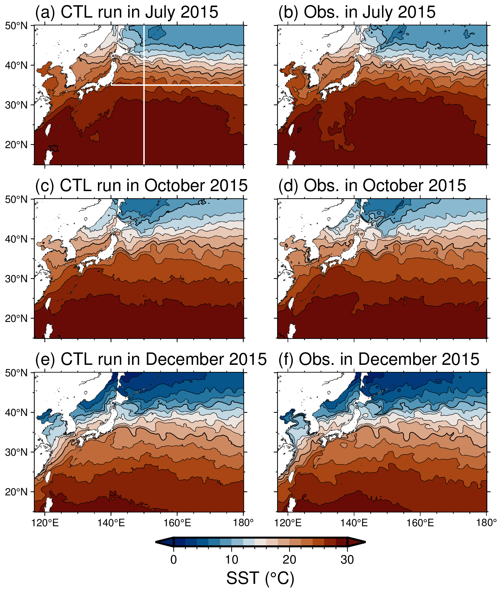
Figure 1 Monthly mean SSTs for (a) July, (c) October, and (e) December 2015 in the CTL run. Panels (b), (d), and (f) are the same as panels (a), (c), and (e), respectively, but for assimilated satellite SSTs. Thin (thick) black contour intervals are 2 (10) ^∘C. The white lines in panel (a) indicate 150^∘ E (35^∘ N) used for the zonal (meridional) sections in Fig. 3.

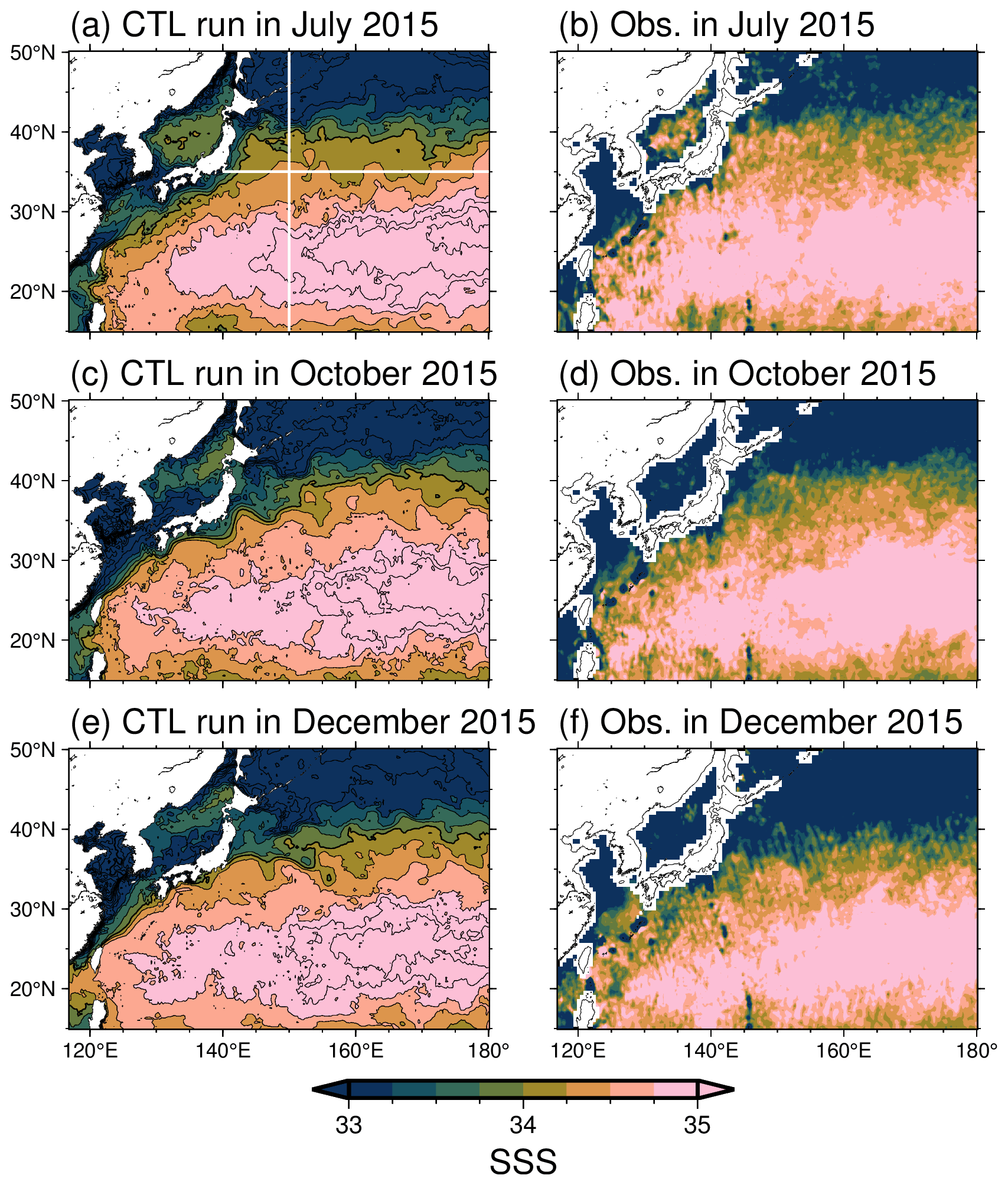
Figure 2 Same as Fig. 1 but for SSS. Thin (thick) black contour intervals are 0.25 (2). In panels (b), (d), and (f), contour intervals are not shown because the satellite observations are noisy.

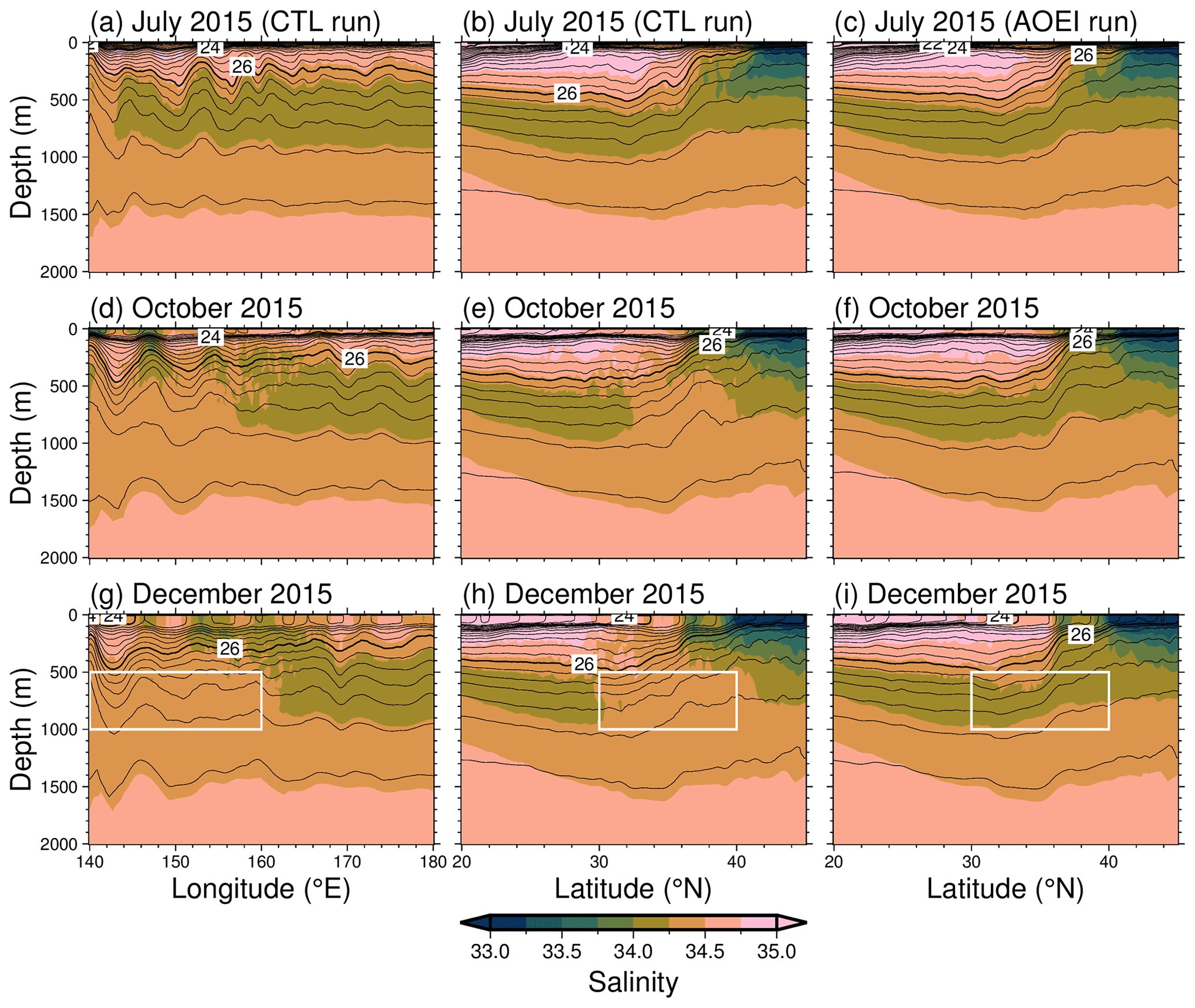
Figure 3 The zonal section of monthly mean salinity (color) and potential density (contours) along 35^∘ N in (a) July, (d) October, and (g) December 2015 in the CTL run. Panels (b), (e), and (h) are the same as panels (a), (d), and (g), respectively, but for the meridional section along 150^∘ E. Panels (c), (f), and (i) are the same as panels (b), (e), and (h), respectively, but for the AOEI run. Thin (thick) contour intervals are 0.25 (2) kg m⁻³. The white box in panels (g), (h), and (i) encloses a longitude (latitude)–depth section of 140–160^∘ E (30–40^∘ N) and 500–1000 m depth.

3.2 Spatiotemporal characteristics of the AOEI application in the surface fields

To investigate how much the AOEI applies to the SST, SSS, and SSH fields, we calculate the monthly mean ratio of the area where the AOEI is applied to the entire system domain (Fig. 4). Application of the AOEI to the SSS field is the highest at around 35 %–40 % of the domain because the instantaneous satellite observations are noisy (cf. Fig. 2; https://smos-diss.eo.esa.int/socat/SMOS_Open, last access: 24 November 2022). The AOEI is also applied to the SST field at a relatively high ratio of 5 %–10 %, whereas the ratio in the SSH field is exceedingly small (less than 0.1 %). This indicates that the AOEI method is applied substantially to the SST and SSS fields but rarely to the SSH field.

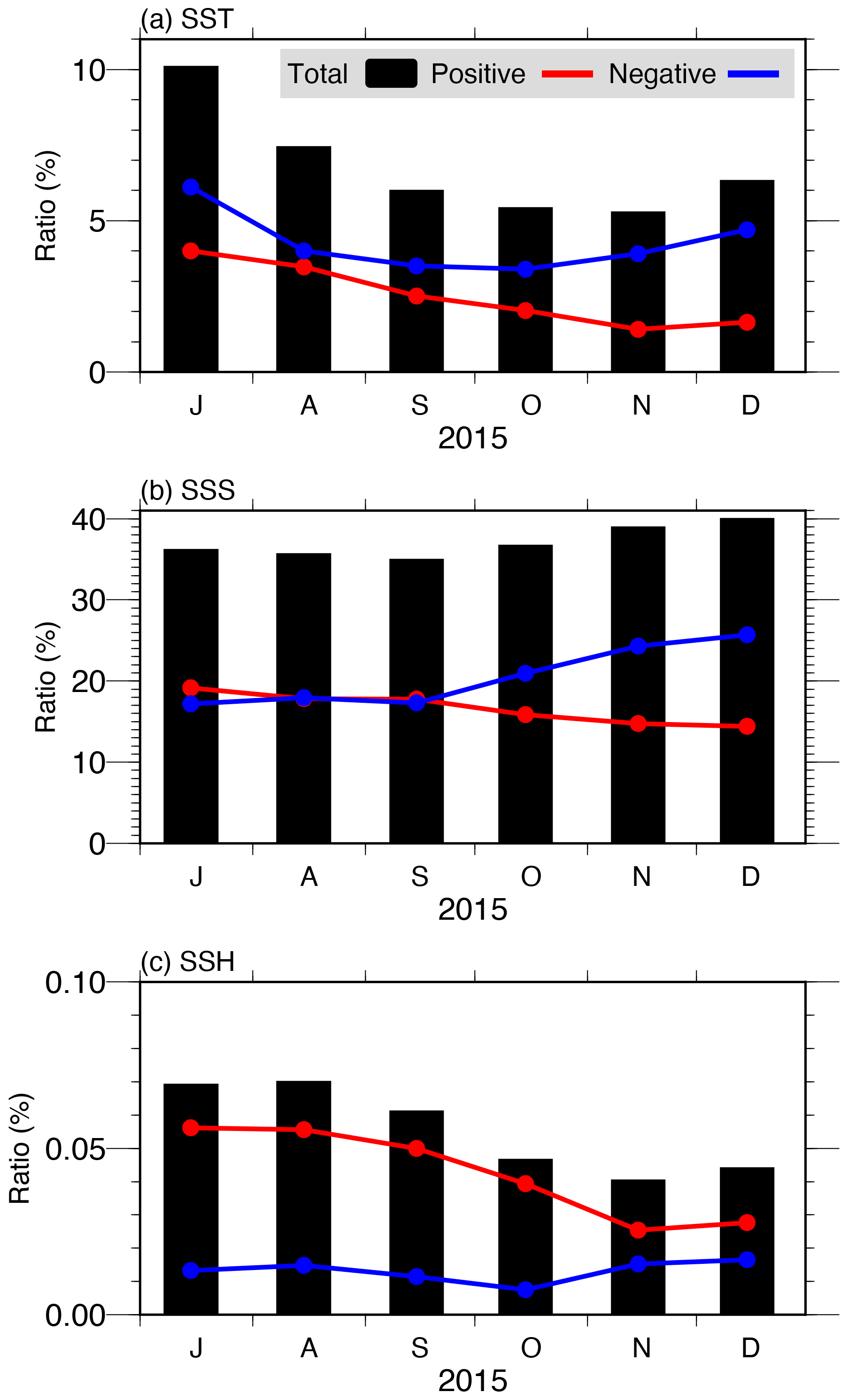
Figure 4 Monthly mean ratio of the area where the AOEI is applied to the system domain in the (a) SST, (b) SSS, and (c) SSH fields in the AOEI run (black bars). Red (blue) lines indicate when the innovation is positive (negative).

We also examine the spatial characteristics of where the AOEI is applied to the SST and SSS fields by calculating the ratio of the period when the AOEI method is applied compared with the total experimental period (Figs. 5, 6). High SST ratios are distributed in the coastal and frontal regions, including the Kuroshio, the KE, and a subpolar front along J1 around 40^∘ N, 150^∘ E (Fig. 5a; Isoguchi et al., 2006; Kida et al., 2015). The SSS ratios are high in the East China Sea, the Sea of Japan, and high-latitude regions (Fig. 6a). The spatial pattern of the positive and negative innovation phases is asymmetric in both the SST and SSS fields (Figs. 5b, c; 6b, c). In the positive innovation phase, the high SST ratios are distributed only along the northeastern coast of Japan at 40–50^∘ N, 140–150^∘ E (Fig. 5b), whereas high SST ratios are more widely distributed in the negative innovation phase, covering coastal and frontal regions (Fig. 5c). In the negative innovation phase, the SSS ratios are higher in the East China Sea, the Sea of Japan, and high-latitude regions (Fig. 6b, c). In the SST and SSS fields, the spatial patterns of the positive forecast biases correspond closely to the high ratios in the negative innovation phase (Figs. 5c, 6c, 7). Therefore, the forecast SST and SSS biases lead to the asymmetry in which the AOEI is applied more during negative innovation phases than during positive phases, as seen in Fig. 4a and b.

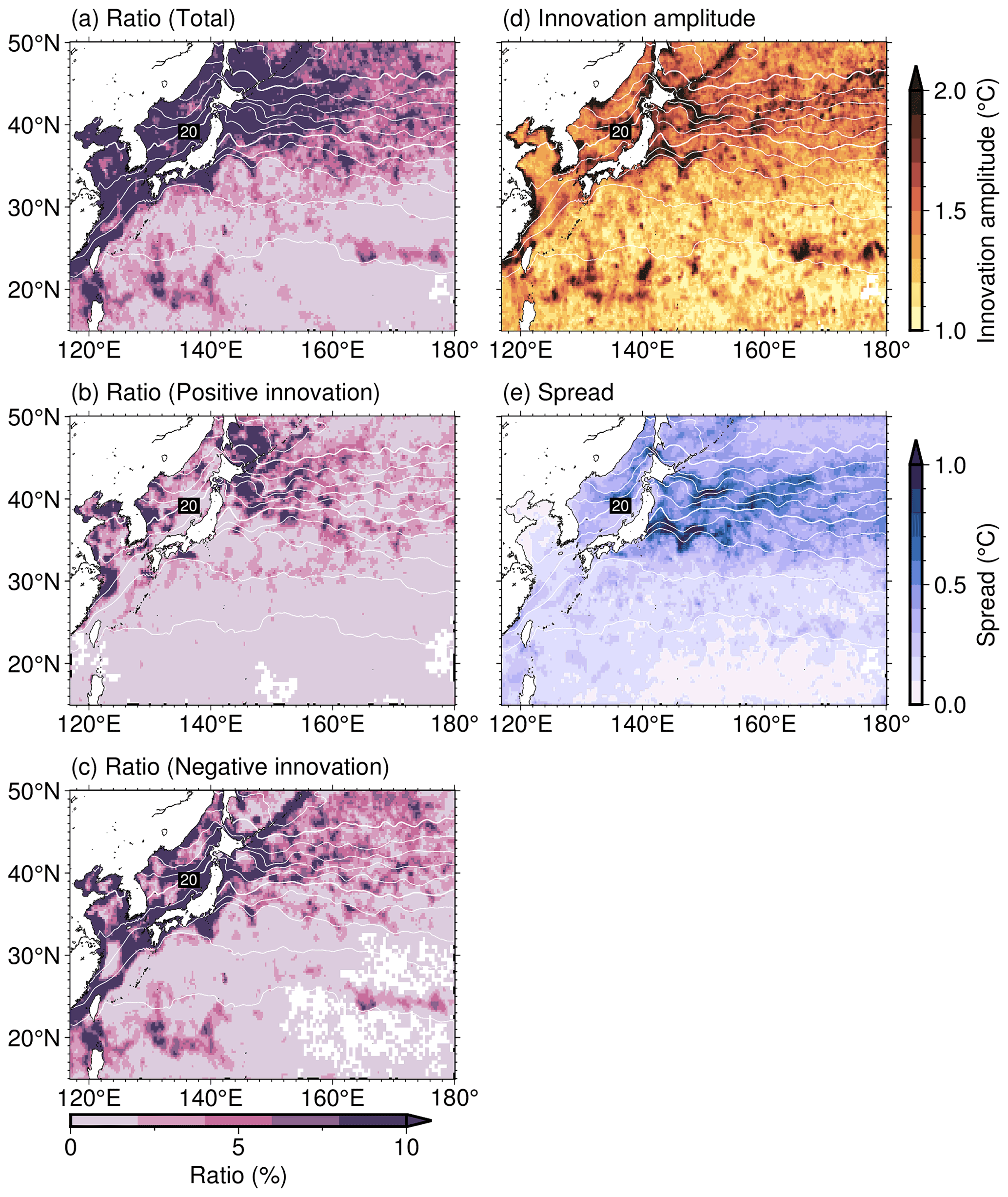
Figure 5 (a) Ratio of the period when the AOEI is applied to the SST compared with the whole experimental period in the AOEI run. Panels (b) and (c) are the same as panel (a) but for when the innovation is positive and negative, respectively. Panels (d) and (e) show the innovation amplitude and ensemble spread averaged during the period when the AOEI is applied, respectively. White contours indicate SST averaged over the whole period. Thin (thick) contour intervals are 2 (10) ^∘C. White areas indicate no AOEI application.

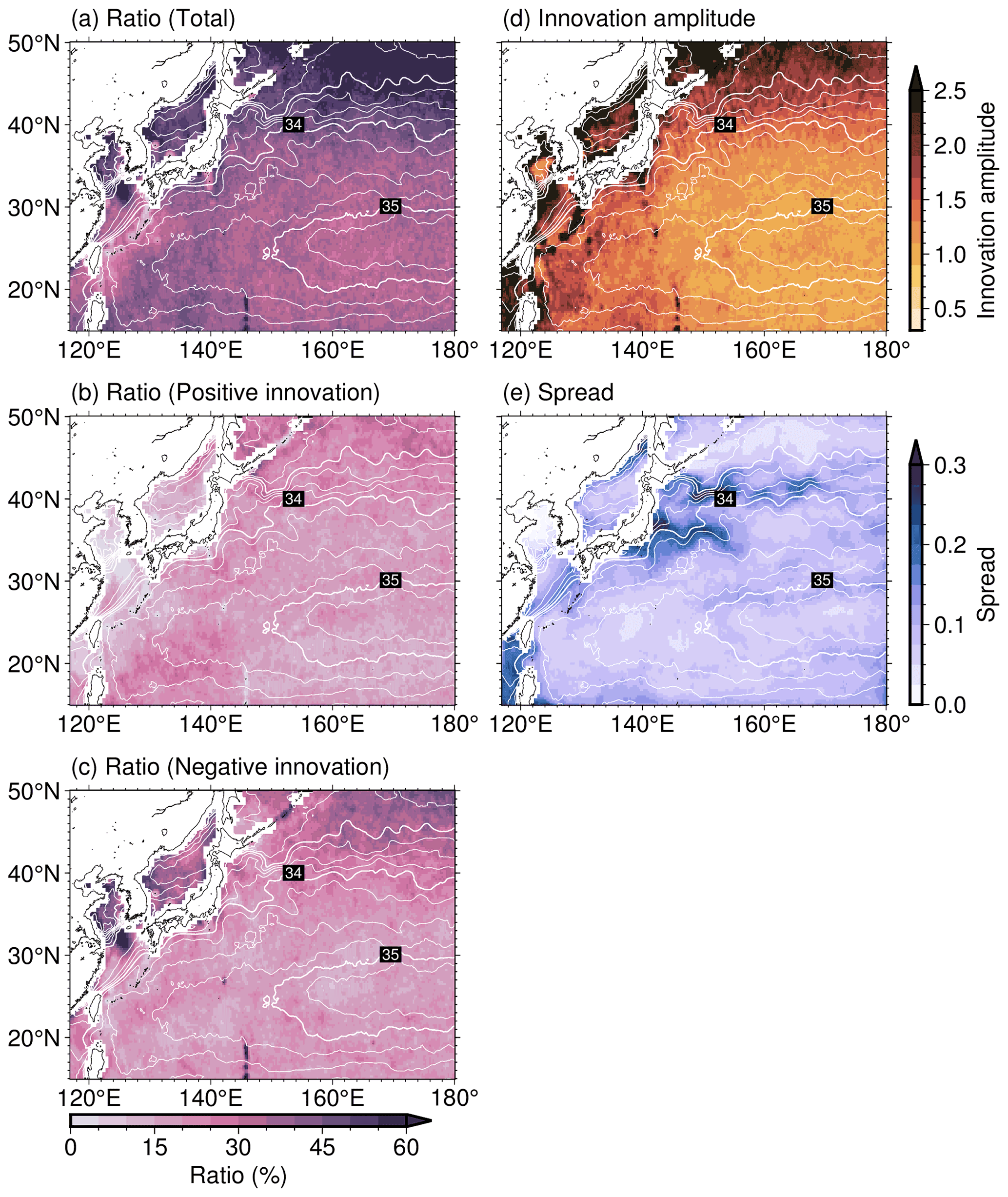
Figure 6 Same as Fig. 5 but for SSS. Thin (thick) contour intervals are 0.25 (1).

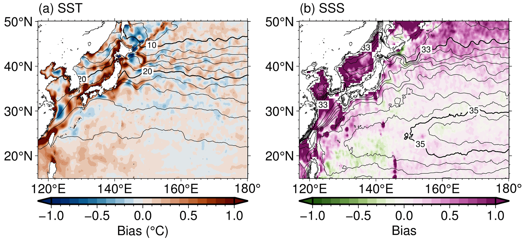
Figure 7 (a) SST and (b) SSS forecast biases (color) and averages (contours) over the whole experimental period in the AOEI run. Thin (thick) contour intervals are 2 (10) ^∘C in panel (a) and 0.25 (2) in panel (b).

In the SST field, large innovation amplitude and forecast ensemble spread are distributed along the KE and the J1 (Fig. 5d, e). In the SSS field, the ensemble spread is large along the KE and J1, where the salinity innovation amplitude is large and exceeds 1.0 (Fig. 6d, e). This demonstrates that large temperature and salinity analysis increments are likely to be generated in the KE and J1 regions if the AOEI is not applied, as in the CTL run.

3.3 Improvements in the salinity structure by the AOEI

We compare monthly temperature and salinity fields between the CTL and AOEI runs at the sea surface and along the 35^∘ N and 150^∘ E sections. In the AOEI run, noisy signals are reduced in the temperature and salinity fields especially in the ocean interior (Fig. 3c, f, i), and the low-salinity water persists in the intermediate layer. The salinity budget analysis indicates that this salinity improvement results from the reduction in the vertical salinity diffusion in the AOEI run relative to the CTL run (see Appendix B for more detail). Figure 8 shows the vertical profile of the vertical diffusivity κ_z averaged over the KE region (30–40^∘ N, 140–160^∘ E) for the whole experimental period and the maximum of the averaged diffusivity over the whole experimental period within 300–1000 m depth. As is consistent with the results of the salinity budget analysis, there is exceedingly large vertical diffusivity at 300–800 m depth around the KE region, which results in salinity degradation induced by strong vertical diffusion in the CTL run. In contrast, the low-salinity water in the intermediate layer persists in the AOEI run because the vertical diffusivity is smaller.

Figure 8 Vertical diffusivity (black), and squared buoyancy frequency (red) and shear (blue) averaged over the KE region (30–40^∘ N, 140–160^∘ E) for the whole experimental period in the (a) CTL and (b) AOEI runs. Maxima of the averaged vertical diffusivity for the whole experimental period within 300–1000 m depth in the (c) CTL and (d) AOEI runs. Black contours show SSH averaged over the whole period. Thin (thick) contour intervals are 0.2 (1) m.

Weak density stratification and strong vertical shear are favorable conditions for the generation of large vertical diffusivity (Davis et al., 2016; Pacanowski and Philander, 1981). To gain dynamical insight into the vertical diffusivity difference between the AOEI and CTL runs, the temporal tendencies of the vertical diffusivity κ_z, the squared buoyancy frequency $N^{\mathrm{2}}=-g/{\mathit{\sigma }}_{\mathit{\theta }}\partial {\mathit{\sigma }}_{\mathit{\theta }}/\partial z$, and the squared vertical shear ${\mathit{u}}_z^{\mathrm{2}}={\left|\partial \mathit{u}/\partial z\right|}^{\mathrm{2}}$ ($\partial {\mathit{\kappa }}_z/\partial t$, $\partial N^{\mathrm{2}}/\partial t$, and $\partial {\mathit{u}}_z^{\mathrm{2}}/\partial t$, respectively) are summed during the positive vertical diffusivity tendency ($\partial {\mathit{\kappa }}_z/\partial t>\mathrm{0})$, and they are then averaged in the KE region (30–40^∘ N, 140–160^∘ E). The buoyancy frequency can be represented as the sum of the contributions from the temperature and salinity vertical gradients ($N_{\mathrm{T}}^{\mathrm{2}}$ and $N_{\mathrm{S}}^{\mathrm{2}}$, respectively):

$$\begin{array}{}\text{(12)}& N^{\mathrm{2}}=-{\displaystyle \frac{g}{{\mathit{\sigma }}_{\mathit{\theta }}}}{\displaystyle \frac{\partial {\mathit{\sigma }}_{\mathit{\theta }}}{\partial z}}=g\left({\mathit{\alpha }}_{\mathrm{T}}{\displaystyle \frac{\partial T}{\partial z}}-{\mathit{\beta }}_{\mathrm{S}}{\displaystyle \frac{\partial S}{\partial z}}\right)\equiv N_{\mathrm{T}}^{\mathrm{2}}+N_{\mathrm{S}}^{\mathrm{2}}.\end{array}$$

Here, α_T (β_S) is the thermal (salinity) expansion coefficient.

Figure 9a and b show that the total vertical diffusivity tendency is smaller in the AOEI run than in the CTL run, which agrees qualitatively with the diffusivity averaged over the whole period (Fig. 8a, b). As is clear from Fig. 9c and d, the total shear tendency is almost zero in both the CTL and AOEI runs. The total buoyancy frequency tendency makes substantial contributions in the CTL and AOEI runs, and its amplitude is smaller in the AOEI run than in the CTL run. As the negative values indicate weakening of the density stratification, the density stratification is less weakened in the AOEI run than in the CTL run. The difference in the total buoyancy frequency tendency between the AOEI and CTL runs is caused by the differences in both the total $\partial N_{\mathrm{T}}^{\mathrm{2}}/\partial t$ and $\partial N_{\mathrm{S}}^{\mathrm{2}}/\partial t$ (Fig. 9e). Although $\partial N_{\mathrm{T}}^{\mathrm{2}}/\partial t$ ($\partial N_{\mathrm{S}}^{\mathrm{2}}/\partial t)$ can be decomposed into the temporal tendency terms of the vertical temperature (salinity) gradient and the thermal (salinity) expansion coefficient, we confirmed that the latter terms are almost zero and have almost no impact on $\partial N_{\mathrm{T}}^{\mathrm{2}}/\partial t$ and $\partial N_{\mathrm{S}}^{\mathrm{2}}/\partial t$. Therefore, the differences in the temperature and salinity vertical gradient tendencies result in less weakening of the density stratification in the AOEI run than in the CTL run.

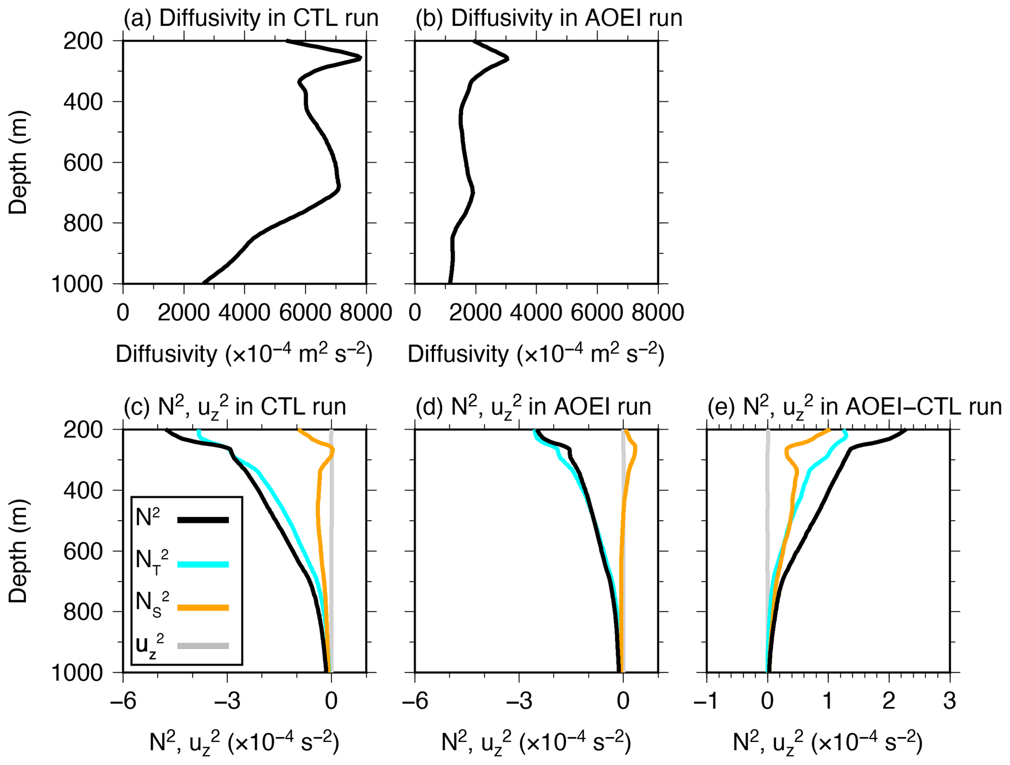
Figure 9 Total vertical diffusivity tendency during the positive vertical diffusivity tendency period averaged over the KE region (30–40^∘ N, 140–160^∘ E) in the (a) CTL and (b) AOEI runs. Panels (c) and (d) are the same as panel (a) but for the squared buoyancy frequency (black) and shear (gray) tendency. Panel (e) is the same as panels (c) and (d) but for the AOEI minus CTL run. In panels (c)–(e), cyan (orange) lines indicate contributions from $\partial N_{\mathrm{T}}^{\mathrm{2}}/\partial t$ ($\partial N_{\mathrm{S}}^{\mathrm{2}}/\partial t$).

To investigate the causes of the differences in the temperature and salinity vertical gradient tendencies between the AOEI and CTL runs, we derive the temperature and salinity stratification tendency equations, respectively, by taking the vertical derivatives of the temperature and salinity budget equations (Eqs. 4 and 5) in the ocean interior:

$$\begin{array}{}\text{(13)}& \begin{array}{rl}{\displaystyle \frac{\partial }{\partial t}}\left({\displaystyle \frac{\partial T}{\partial z}}\right)& ={\displaystyle \frac{\partial }{\partial z}}\left\{\mathbf{\nabla }\cdot \left(\mathit{\kappa }\circ \mathbf{\nabla }T\right)\right\}-{\displaystyle \frac{\partial }{\partial z}}(\mathit{v}\cdot \mathbf{\nabla }T)\\ & +{\displaystyle \frac{\mathrm{1}}{{\mathit{\rho }}_{\mathrm{0}}{c}_{\mathrm{p}}}}{\displaystyle \frac{\partial q_{\mathrm{sw}}}{\partial z}}+{\displaystyle \frac{\partial }{\partial z}}\left(T\mathrm{increment}\right),\end{array}\end{array}$$

and

$$\begin{array}{}\text{(14)}& \begin{array}{rl}{\displaystyle \frac{\partial }{\partial t}}\left({\displaystyle \frac{\partial S}{\partial z}}\right)& ={\displaystyle \frac{\partial }{\partial z}}\left\{\mathbf{\nabla }\cdot \left(\mathit{\kappa }\circ \mathbf{\nabla }S\right)\right\}-{\displaystyle \frac{\partial }{\partial z}}(\mathit{v}\cdot \mathbf{\nabla }S)\\ & +{\displaystyle \frac{\partial }{\partial z}}\left(S\mathrm{increment}\right).\end{array}\end{array}$$

As in the total vertical diffusivity tendency calculated above, each term in Eqs. (13) and (14) is summed when $\partial {\mathit{\kappa }}_z/\partial t>\mathrm{0},$ and then averaged over the KE region (30–40^∘ N, 140–160^∘ E) (Fig. 10). We note that positive values in Eqs. (13) and (14) indicate opposite effects on the density stratification: a positive temperature (salinity) vertical gradient tendency strengthens (weakens) the density stratification.

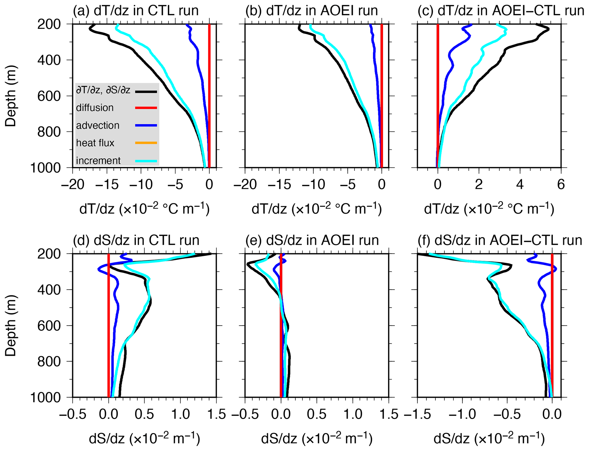
Figure 10 Panels (a)–(c) are the same as Fig. 9 but for each term of the temperature stratification tendency equation (Eq. 13): the temperature gradient tendency term (the LHS term; black), the temperature diffusion gradient term (the first term on the RHS; red), the temperature advection gradient term (the second term on the RHS; blue), the shortwave penetration gradient term (the third term on the RHS; orange), and the temperature increment gradient term (the last term on the RHS; cyan). Panels (d)–(f) are the same as panels (a)–(c) but for the salinity stratification tendency equation (Eq. 14). In panels (a)–(c), we note that the shortwave penetration gradient term is almost zero and overlaps with the temperature diffusion gradient term.

In the CTL and AOEI runs, the temperature gradient tendency term (the left-hand side (LHS) term of Eq. 13) is negative and indicates that the temperature and density stratification are weakened at all depths (Fig. 10a, b). The amplitude of this term is smaller in the AOEI run than in the CTL run, and thus the temperature and density stratification is less weakened. As shown in Fig. 10c, the difference in the temperature gradient tendency between the AOEI and CTL runs is due mainly to the temperature analysis increment gradient term (the last term on the right-hand side (RHS) of Eq. 13) and in part to the advection gradient term (the second term on the RHS of Eq. 13), whereas the diffusion and shortwave penetration gradient terms (the first and third terms on the RHS of Eq. 13, respectively) make almost no contribution.

In the CTL run, the salinity gradient tendency term (the LHS term of Eq. 14) indicates that the salinity (density) stratification is strengthened (weakened) at all depths (Fig. 10d). In the AOEI run, the salinity (density) stratification is weakened (strengthened) at 200–400 m depth and slightly strengthened (weakened) at 400–1000 m depth (Fig. 10e). The salinity gradient tendency term is smaller in the AOEI run than in the CTL run at all depths, and thus the salinity (density) stratification is less strengthened (weakened) in the AOEI run relative to the CTL run (Fig. 10f). The difference in the salinity analysis increment gradient terms (the last term on the RHS of Eq. 14) between the AOEI and CTL runs dominates that in the salinity gradient tendency term, whereas the differences between the diffusion and advection gradient terms (the second and third terms on the RHS of Eq. 14, respectively) have little influence. This indicates that less strengthening (weakening) of the salinity (density) stratification in the AOEI run relative to the CTL run is due to the smaller salinity analysis increment. The impacts of the SST, SSS, and SSH assimilation are limited to between the surface and about 370 m depth because of the prescribed vertical localization scale of 100 m described in Sect. 2.2, and consequently only in situ temperature and salinity assimilation generates the analysis increments in the intermediate layer.

The AOEI contributes to maintaining the density stratification by reducing the temperature and salinity analysis increments and preventing the occurrence of large vertical diffusivity that degrades low-salinity water in the intermediate layer around the KE region. In the CTL run, the salinity analysis increments restore the degraded low-salinity water (see Appendix A) but lead to degradation via the formation of large vertical diffusivity at the same time. Thus, it seems that positive feedback exists that may degrade the salinity structure.

3.4 Improvement in the geostrophic balance and accuracy by the AOEI

In this subsection, we investigate the impacts of the AOEI on the geostrophic balance and accuracy. Figure 11 shows ΔNBE averaged over the whole period in the CTL and AOEI runs. In the CTL run, ΔNBE is large in the midlatitude regions, especially along the KE (Fig. 11a). In the AOEI run, ΔNBE is smaller than in the CTL run for the entire domain (Fig. 11b). The spatiotemporally averaged ΔNBE over the whole experimental period and domain is 0.57 × 10⁻¹⁰ and 0.35 × 10⁻¹⁰ s⁻² for the CTL and AOEI runs, respectively, and the balance is significantly improved in the AOEI run relative to the CTL run. This is probably because the analysis increments are smaller in the AOEI run than in the CTL run.

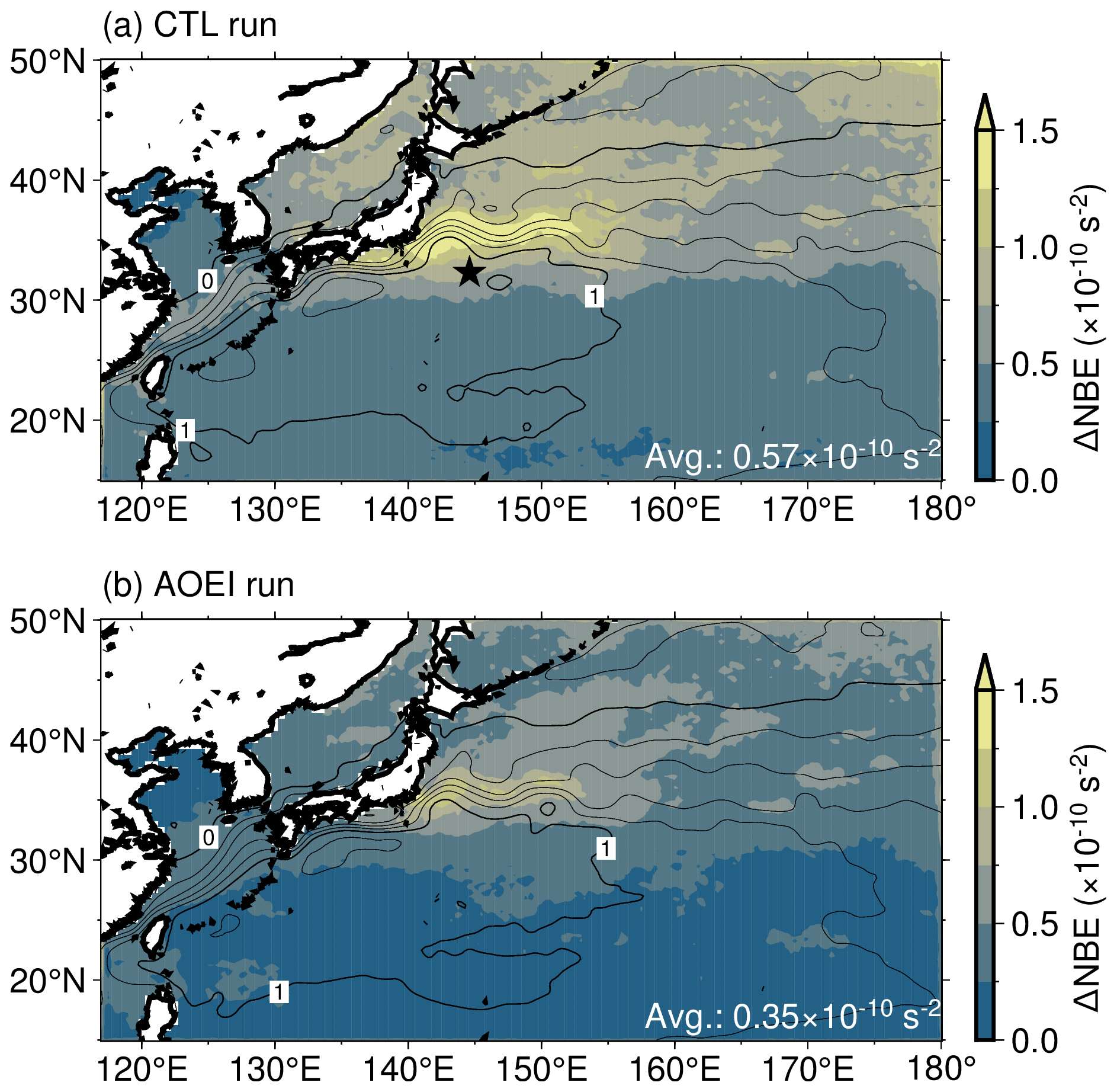
Figure 11 ΔNBE (color) and SSH (contours) averaged over the whole experimental period for the (a) CTL and (b) AOEI runs. Thin (thick) contour intervals are 0.2 (1) m. Spatiotemporally averaged ΔNBE over the whole period and domain is shown in the lower right-hand corners. The black star in panel (a) denotes the position of the KEO buoy.

To investigate the analysis accuracy in the ocean interior, we calculate the RMSDs of the CTL, AOEI, and 1.5Terr runs relative to in situ temperature, salinity, and horizontal velocity observations from the KEO buoy south of the KE (Figs. 11a, 12). Results are only presented for the temperature and salinity because no significant results are obtained for the horizontal velocities. The RMSDs for both temperature and salinity are smaller in the AOEI run than in the CTL run, and the AOEI run provides significant temperature (salinity) improvements at 0–150 m (50–400 m) depth relative to the CTL run. This is probably because the AOEI suppresses the development of the strong vertical diffusion that leads to the salinity degradation and because of the improvement in the geostrophic balance. We have confirmed that the AOEI run also has smaller temperature (salinity) RMSDs than the 1.5Terr run throughout the depth except for two observation points at 225 and 275 m (150 and 525 m) depth. Therefore, among the experiments, the AOEI run is the best for the accuracy of temperature and salinity south of the KE.

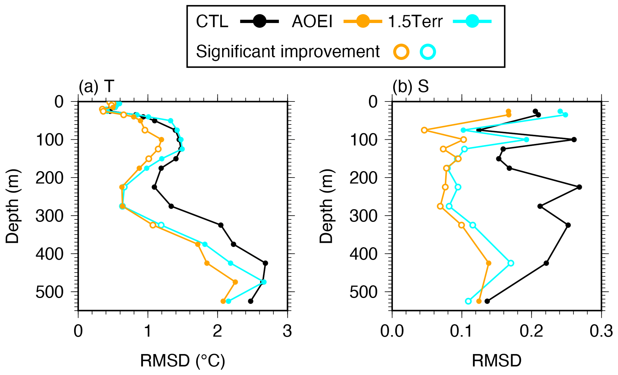
Figure 12 (a) Temperature and (b) salinity RMSDs averaged over the whole experimental period at the KEO buoy in the CTL (black), AOEI (orange), and 1.5Terr (cyan) runs. Open circles indicate significant improvement in the AOEI and 1.5Terr runs relative to the CTL run.

We also investigate the analysis accuracy of the SSH, surface flow, and SST fields, respectively, calculating the spatiotemporally averaged RMSDs relative to the SSH and SSHA datasets from the AVISO, relative to in situ surface horizontal velocity observations from the drifter buoys, and relative to Himawari-8 SSTs (Fig. 13). Although the AOEI run slightly degrades the SST accuracy relative to the CTL run (Fig. 13e), the RMSDs in the AOEI run are smaller for all other variables, and they indicate significant improvements except for surface meridional velocity (Fig. 13a, b, c, d). The improvement in the surface-flow field in the AOEI run would result from the better geostrophic balance and accuracy of the density structure in the ocean interior. Relative to the 1.5Terr run, the AOEI run improves the accuracy for all variables.

Figure 13 RMSDs of the CTL, AOEI, and 1.5Terr runs relative to (a) SSH and (b) SSHA datasets from the AVISO, relative to in situ surface (c) zonal and (d) meridional velocity from drifter buoys, and relative to (e) Himawari-8 SSTs averaged over the whole domain and period. Black dots indicate the ensemble spread in the observation space. We note that the ranges of the vertical axis are different between the RMSDs and ensemble spreads.

Kurihara et al. (2016), for example, show that the RMSDs of the Himawari-8 SSTs relative to the buoys are about 0.5 ^∘C and are larger in the higher-latitude regions with a larger zenith angle and that observation error variances have substantial contributions to the RMSDs. However, the ensemble spreads are much smaller than the RMSDs for all variables (Fig. 13). We have found that the ensemble spreads in the subtropical region appear to be under-dispersive even if the perturbed atmospheric and lateral boundary conditions are applied (cf. Figs. 5e and 6e). Methods to inflate the ensemble spread more would be required for further improvements in the accuracy, but this will be a future issue.

4 Summary

We have implemented the AOEI with the sbPOM-LETKF ocean data assimilation system and conducted sensitivity experiments to investigate the impacts on the low-salinity NPIW around the KE region, the geostrophic balance, and the analysis accuracy. In the CTL run, the large analysis increments by in situ temperature and salinity assimilation weaken the density stratification. The resulting exceedingly large vertical diffusivity induces the strong vertical diffusion that breaks the low-salinity structure in the NPIW around the KE region. The salinity analysis increment contributes to restoring the low-salinity water but, at the same time, causes salinity degradation by generating strong vertical diffusion. Therefore, a positive feedback appears to occur, degrading the salinity structure.

The AOEI decreases the temperature and salinity analysis increments around the KE region by adaptively inflating the temperature and salinity observation errors, respectively. As a result, the AOEI mitigates the salinity degradation seen in the CTL run; therefore, the low-salinity water is maintained in the AOEI run. In addition, the AOEI significantly improves the geostrophic balance, probably because of the reduction in the analysis increments. Moreover, the AOEI prevents the development of strong vertical diffusion and improves the accuracy of temperature and salinity in the ocean interior. Furthermore, the improvements in the geostrophic balance and density structure in the ocean interior contribute to more accurate SSH and surface-flow fields. In summary, this study demonstrates the positive impacts of the AOEI on the balance and accuracy of the temperature, salinity, and surface-flow fields.

As our available computational resources were limited, we fixed the tuning parameter of the RTPP, perturbed atmospheric forcing, ensemble size, localization scale, and prescribed observation errors. Further experiments to explore more optimal settings are required, and this will be investigated in the future. Coastal data assimilation systems with a high horizontal resolution might reach the stage where they capture sub-mesoscale phenomena, such as filaments with strong temperature and salinity gradients. For such systems, the position errors of fronts, eddies, and filaments might cause degradation as seen in the CTL run. Furthermore, low-salinity water is distributed in the intermediate layer in western boundary current regions in all ocean basins. Consequently, we would expect that this study will be helpful for improving and developing EnKF-based ocean data assimilation systems. Minamide and Zhang (2017) noted that the AOEI has the advantage of being easily implemented with various EnKF-based systems, and this study serves as a good example of the usefulness of the AOEI. We are currently constructing high-resolution reanalysis datasets in the western North Pacific and Maritime Continent regions based on this system, and we plan to develop (near-)real-time ensemble forecast systems.

Appendix A: The cause of salinity degradation in the CTL run

To investigate the cause of the salinity degradation in the CTL run, we calculate the salinity budget equation (Eq. 5) in the intermediate layer around the KE region (30–40^∘ N, 140–160^∘ E; 500–1000 m depth; white boxes in Fig. 3g, h). Figure A1a indicates that the salinity tendency term (the LHS term of Eq. 5) is positive and corresponds to the salinity increase shown in Fig. 3a, b, d, e, g, and h. The positive salinity tendency term is caused mainly by the diffusion term (the first term on the RHS of Eq. 5) and partly by the advection term (the second term on the RHS of Eq. 5). The diffusion term is dominated only by the vertical diffusion, and the horizontal diffusion makes almost no contribution (Fig. A1b). The advection term consists of different components in different months during the experimental period (Fig. A1c): meridional advection in July, zonal and meridional advection in August, and zonal and vertical advection in September–December 2015. In contrast, the salinity analysis increment term (the last term on the RHS of Eq. 5) has only a minor impact but plays a role in restoring the low-salinity water. Therefore, the vertical diffusion is the main cause of the salinity degradation in the intermediate layer around the KE region.

Figure A1 (a) Monthly mean for each term in the salinity budget equation (Eq. 5) averaged over the KE region in the intermediate layer (30–40^∘ N, 140–160^∘ E; 500–1000 m depth) in the CTL run: the salinity tendency term (the LHS term; black bars), the salinity diffusion term (the first term on the RHS; red line), the salinity advection term (the second term on the RHS, blue line), and the salinity analysis increment term (the last term on the RHS; gray line). Panels (b) and (c) are the same as panel (a) but for the salinity diffusion and advection terms (black bars), respectively, as well as the zonal (orange lines), meridional (cyan lines), and vertical (green lines) components.

Appendix B: The cause of salinity improvement in the AOEI run

To investigate the cause of the salinity improvement in the AOEI run relative to the CTL run, we calculate the salinity budget equation (Eq. 5) difference between the AOEI and CTL runs (Fig. B1):

$$\begin{array}{}\text{(B1)}& \mathrm{\Delta }\left({\displaystyle \frac{\partial S}{\partial t}}\right)=\mathrm{\Delta }\mathit{\{}\mathbf{\nabla }\cdot \left(\mathit{\kappa }\circ \mathbf{\nabla }S\right)\mathit{\}}-\mathrm{\Delta }(\mathit{v}\cdot \mathbf{\nabla }S)+\mathrm{\Delta }\left(S\mathrm{increment}\right),\end{array}$$

where Δ indicates the AOEI run minus the CTL run. The salinity tendency difference term (the LHS term of Eq. B1) indicates that the salinity structure is maintained in the AOEI run by suppressing the salinity increase throughout the experimental period (Fig. B1a). The diffusion and advection difference terms (the first and second terms on the RHS of Eq. B1, respectively) contribute almost equally to the salinity tendency difference term. The diffusion difference term is dominated by only the vertical diffusion difference, whereas the advection difference term is dominated by different components in different months: by the meridional advection difference in July, by all advection differences in August–September, and by vertical and partly zonal advection differences in October–December 2015. The reduction in the vertical diffusion is, therefore, the main cause of the improvement for low-salinity water in the AOEI run relative to the CTL run.

Figure B1 (a) Monthly mean for each term for the difference between the AOEI and CTL runs in the salinity budget equation (Eq. B1): the salinity tendency difference term (the LHS term; black bars), the salinity diffusion difference term (the first term on the RHS; red line), the salinity advection difference term (the second term on the RHS; blue line), and the salinity analysis increment difference term (the last term on the RHS; gray line). Panels (b) and (c) are the same as (a) but for the salinity diffusion and advection difference terms (black bars), respectively, as well as the zonal (orange lines), meridional (cyan lines), and vertical (green lines) components.