the Creative Commons Attribution 4.0 License.
the Creative Commons Attribution 4.0 License.
 | 01 Feb 2022
The Earth Model Column Collaboratory (EMC2) v1.1: an open-source ground-based lidar and radar instrument simulator and subcolumn generator for large-scale models
Robert C. Jackson
Ann M. Fridlind
Andrew S. Ackerman
Scott Collis
Johannes Verlinde
Jiachen Ding
Climate models are essential for our comprehensive understanding of Earth's atmosphere and can provide critical insights on future changes decades ahead. Because of these critical roles, today's climate models are continuously being developed and evaluated using constraining observations and measurements obtained by satellites, airborne, and ground-based instruments. Instrument simulators can provide a bridge between the measured or retrieved quantities and their sampling in models and field observations while considering instrument sensitivity limitations. Here we present the Earth Model Column Collaboratory (EMC2), an open-source ground-based lidar and radar instrument simulator and subcolumn generator, specifically designed for large-scale models, in particular climate models, but also applicable to high-resolution model output. EMC2 provides a flexible framework enabling direct comparison of model output with ground-based observations, including generation of subcolumns that may statistically represent finer model spatial resolutions. In addition, EMC2 emulates ground-based (and air- or space-borne) measurements while remaining faithful to large-scale models' physical assumptions implemented in their cloud or radiation schemes. The simulator uses either single particle or bulk particle size distribution lookup tables, depending on the selected scheme approach, to perform the forward calculations. To facilitate model evaluation, EMC2 also includes three hydrometeor classification methods, namely, radar- and sounding-based cloud and precipitation detection and classification, lidar-based phase classification, and a Cloud Feedback Model Intercomparison Project Observational Simulator Package (COSP) lidar simulator emulator. The software is written in Python, is easy to use, and can be straightforwardly customized for different models, radars, and lidars.
Following the description of the logic, functionality, features, and software structure of EMC2, we present a case study of highly supercooled mixed-phase cloud based on measurements from the U.S. Department of Energy Atmospheric Radiation Measurement (ARM) West Antarctic Radiation Experiment (AWARE). We compare observations with the application of EMC2 to outputs from four configurations of the NASA Goddard Institute for Space Studies (GISS) climate model (ModelE3) in single-column model (SCM) mode and from a large-eddy simulation (LES) model. We show that two of the four ModelE3 configurations can form and maintain highly supercooled precipitating cloud for several hours, consistent with observations and LES. While our focus is on one of these ModelE3 configurations, which performed slightly better in this case study, both of these configurations and the LES results post-processed with EMC2 generally provide reasonable agreement with observed lidar and radar variables. As briefly demonstrated here, EMC2 can provide a lightweight and flexible framework for comparing the results of both large-scale and high-resolution models directly with observations, with relatively little overhead and multiple options for achieving consistency with model microphysical or radiation scheme physics.
- Article
(10085 KB) - Full-text XML
- BibTeX
- EndNote


The representation of cloud processes in large-scale models is continuously advancing, conceptually, and in the level of details and complexity implemented in the micro- and macro-physical schemes (e.g., Lin et al., 2019; Cesana et al., 2019). These improvements are reflected in the accuracy of the resulting model output (e.g., Klein et al., 2013; Lin et al., 2019; Myers et al., 2021; Wang et al., 2019), yet results still show large inter-model variability (e.g., Zelinka et al., 2020). This variability results from, among other sources, model weaknesses concerning their ability to predict atmospheric state variables and processes such as cloud geometrical and optical thicknesses (e.g., Cesana and Waliser, 2016; Klein et al., 2013), formation and transition of marine stratocumulus clouds (e.g., Rémillard and Tselioudis, 2015; Lin et al., 2014; Cesana et al., 2019), and the formation and maintenance of supercooled water (e.g., Cesana et al., 2012; Tan and Storelvmo, 2016; Silber et al., 2019b).
Meaningful model evaluation benefits from a direct (“apples-to-apples”) comparison with observations (e.g., Bodas-Salcedo et al., 2014; Suzuki et al., 2015). For the evaluation of cloud representation, model output is often compared with active remote-sensing measurements from instrumentation such as lidars and radars, which provide information on the spatial structure of clouds and some direct indications about active microphysical processes. However, model evaluation is challenging because of observational detectability constraints (e.g., signal extinction) and lack of retrievals or large uncertainties in some microphysical and atmospheric state quantities by these instruments, for example, hydrometeor number concentration or water content. In addition, spatial resolution differences between a model's output and an observing instrument's measurement resolution present an additional difficulty.
To bridge the gap between large-scale models such as weather or climate models and active remote-sensing observations, instrument simulators with different purposes have been developed to estimate observed parameters using model output. For example, the Cloud-resolving model Radar SIMulator (CR-SIM; Oue et al., 2020) was developed to emulate zenith-pointing and scanning radar and lidar variables using high-resolution model output, with considerations of hydrometeor shape and the resulting scattering calculations (see also Mech et al., 2020). The Cloud Feedback Model Intercomparison Project Observational Simulator Package (COSP; Bodas-Salcedo et al., 2011; Swales et al., 2018), on the other hand, was developed to operate over large-scale model output targeting satellite data as observational constraints, although expansions for the emulation of ground-based radars and lidars have been developed (e.g., Zhang et al., 2018; Kuma et al., 2020). Among a variety of reasons such as the demanding computation associated with the emulation of satellite measurements and the ability to use and output detailed data to and from simulators, COSP is typically implemented on-line into models' code to facilitate output.
To account for spatial resolution discrepancies, which are typically accentuated in the case of large-scale models due to their coarser resolution, some model evaluation studies and forward simulators emulate a higher spatial resolution by generating subcolumns (e.g., Bodas-Salcedo et al., 2008, 2011; Chepfer et al., 2008; Klein and Jakob, 1999; Lamer, 2019; Stephens et al., 2010; Swales et al., 2018; Webb et al., 2001). Statistics calculated using multiple generated subcolumns, which are nominally faithful to the processed model's physics, can be directly compared with the associated observations, thereby mitigating spatial resolution biases and errors.
Here we present the Earth Model Column Collaboratory (EMC2), an open-source ground-based lidar and radar simulator and subcolumn generator, which is designed to operate over large-scale model output while being faithful to the physics implemented in models' microphysics or radiation schemes but can also be applied to high-resolution model output. EMC2 enables detailed evaluation of atmospheric thermodynamic profile and cloud properties extracted from local, regional, and global simulation outputs against long-term ground-based, air- or space-borne datasets. The software is written in Python, allowing quick installation and providing customizable operation (for scattering calculations, etc.). In Sect. 2, we briefly illustrate the Python code and software followed by a detailed description of the subcolumn generator, the forward calculations, and classification routines currently implemented in EMC2. In Sect. 3 we demonstrate the use of EMC2 by comparing observations of a case study of highly supercooled drizzling cloud over West Antarctica (see Silber et al., 2019a) with application of EMC2 to outputs from a large-eddy simulation (LES) and the NASA Goddard Institute for Space Studies (GISS) ModelE3 climate model (see Cesana et al., 2019) in single-column model (SCM) mode. Finally, Sect. 4 provides a summary of the code features and case study demonstration.
2.1 Software description
EMC2 depicts a workflow for comparing forward calculated radar or lidar variables generated from large-scale model output with radar or lidar measurements. Figure 1 shows a flowchart example of this workflow for using EMC2 to compare ModelE3's output with high spectral resolution lidar (HSRL) measurements. The workflow starts with the Model class incorporated within the emc2.core module. The Model class contains model output field namelists and default hydrometeor parameters (Table 1). Using Python's class inheritance, EMC2 allows the creation of a custom class specifying a given model's namelists and parameters (a ModelE3 class in this example), which ensures that the model output can be standardized and used by the other modules in EMC2. Once loaded through the Model class internal methods, model output data are stored within the Model object using the xarray dataset module (Hoyer and Hamman, 2017).
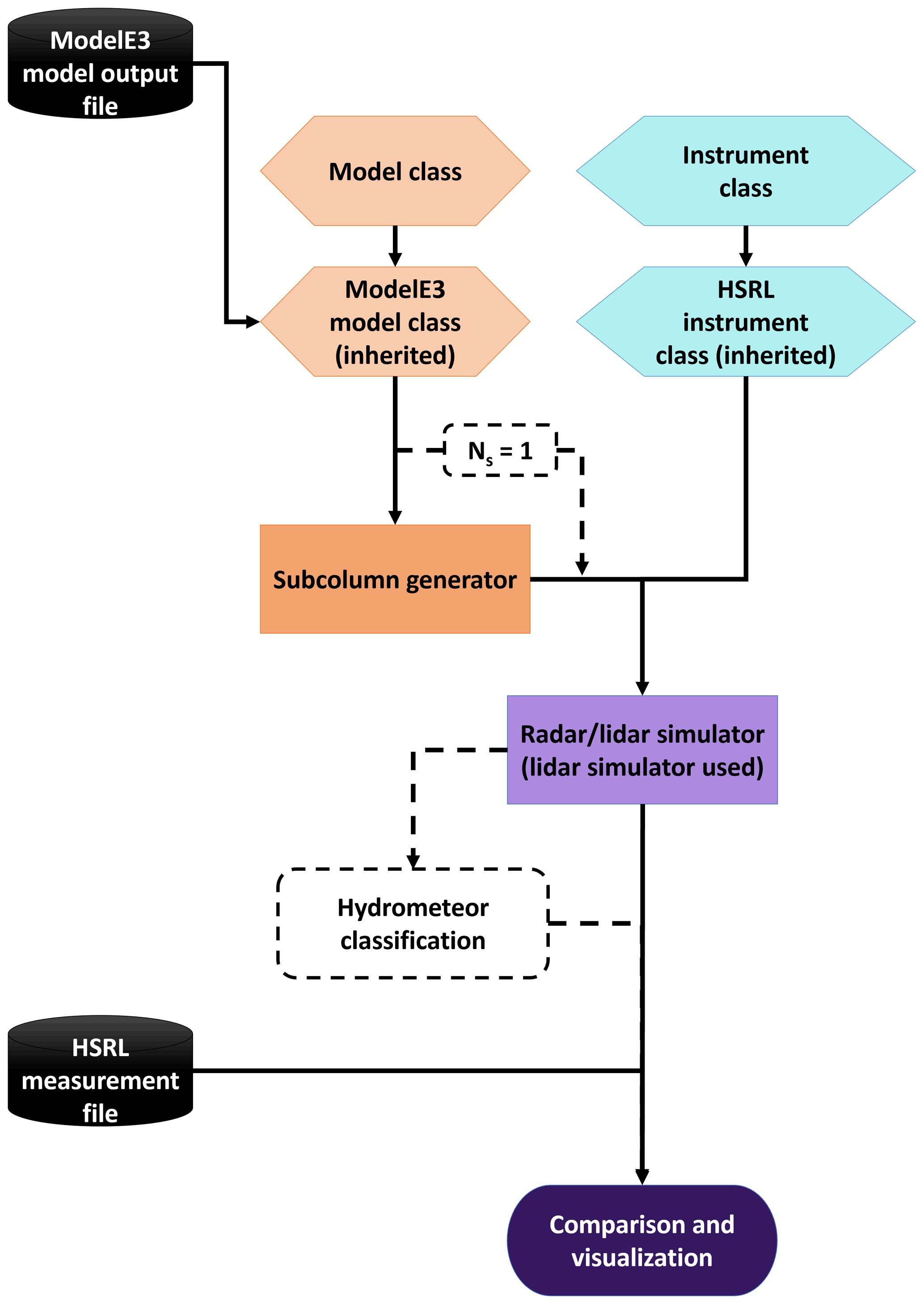
Figure 1Standard workflow of EMC2 utilization for direct comparison between observations and model output. The flowchart exemplifies the use of EMC2 to compare the NASA GISS ModelE3 climate model output with corresponding high spectral resolution lidar (HSRL) measurements. Ns designates the specified number of subcolumns.
The Model object is then input to the subcolumn generator (Sect. 2.2). Note that subcolumn generator processing can be practically skipped by setting the number of subcolumns (Ns) to 1. The results of the subcolumn generator are stored in the xarray dataset contained within the Model object. Here, we introduce the Instrument class. Similar to the Model class, the Instrument class contains relevant information about the instrument being simulated (some of which is listed in Table 2) as well as the single-particle and bulk scattering calculation lookup tables (LUTs) (see Sect. 2.3 and 2.4). Currently, zenith-pointing instrument properties and scattering calculation LUTs are available for various lidars and radars operated by the Department of Energy (DOE) Atmospheric Radiation Measurement (ARM) climate research facility: the elastic micropulse lidar (MPL) and HSRL, both operating at a wavelength of 532 nm (e.g., Flynn et al., 2007; Eloranta, 2005), the 910 nm CL31 ceilometer (Morris, 2016), the 1064 nm HSRL elastic channel (see Razenkov and Eloranta, 2018), the elastic channel of ARM's Raman lidar operating at 355 nm (e.g., Newsom, 2009), the C-band scanning ARM precipitation radar (C-SAPR; starting in EMC2 v. 1.2; Widener and Bharadwaj, 2012), the X-band scanning ARM cloud radar (XSACR; Widener et al., 2012b), the Ka-band ARM zenith radar (KAZR; Widener et al., 2012a), and the W-band ARM cloud radar (WACR and M-WACR; Widener and Johnson, 2006). Similar to the Model class, the Instrument class allows EMC2 to be tailored to other radars and lidars deployed at different sites, which does not confine the analysis of measurements and model output to specific ARM instruments or sites, as long as the required parameters and suitable scattering LUTs are provided. Thus, the various parameters mentioned in the next subsections (e.g., all parameters shown in Tables 1 and 2) as well as the LUTs can be easily specified and set to match configurations and assumptions implemented in different large-scale models, as well as complex scattering models more commonly implemented in cloud-resolving and LES models.
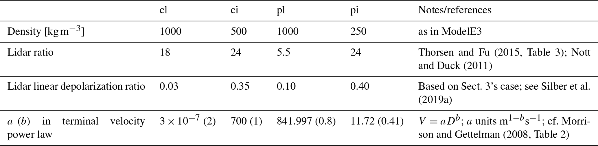
Table 1Hydrometeor class parameter values implemented in EMC2.
Following the subcolumn generator process, the Instrument and Model objects are then input to the lidar (Sect. 2.3) or radar (Sect. 2.4) simulators (lidar simulator in the case of Fig. 1). The forward calculation results are stored in the same xarray dataset in the Model object. Simulated hydrometeor classification (Sect. 2.5) can be performed following the completion of the forward calculations and stored in the xarray dataset. For comparison and visualization of these results, EMC2 uses the Atmospheric Community Toolkit (ACT; Theisen et al., 2020). Thus, a SubcolumnDisplay object, inherited from ACT's Display object, contains the necessary methods for quick visualization of the simulated instrument variables. In addition, the SubcolumnDisplay object also contains several internal methods for generating curtain and profile plots of observational and simulated data stored in the Instrument or Model objects, allowing masking of simulated signals below instrument detectability, for example. The figures presented in the next section (Sect. 3) show examples of EMC2's visualization capabilities. Finally, since the data are in the xarray dataset format, EMC2 also contains all of xarray's analysis and visualization capabilities for these simulated datasets.
Table 2Radar instruments and some of their characteristics currently implemented in EMC2. The ARM SGP, ENA, NSA, AWR, and MOS site abbreviations denote the Southern Great Plains, Eastern North Atlantic, North Slope of Alaska, the AWARE campaign (at McMurdo Station, Antarctica), and the Multidisciplinary Drifting Observatory for the Study of Arctic Climate (MOSAiC) Expedition, respectively. The calculations of the minimum detectable signal () for KAZR are based on the analysis in Silber et al. (2018a). All values correspond to 2 s integration time except for the AWR and MOS WACR, the values of which correspond to 0.2 s integration time.
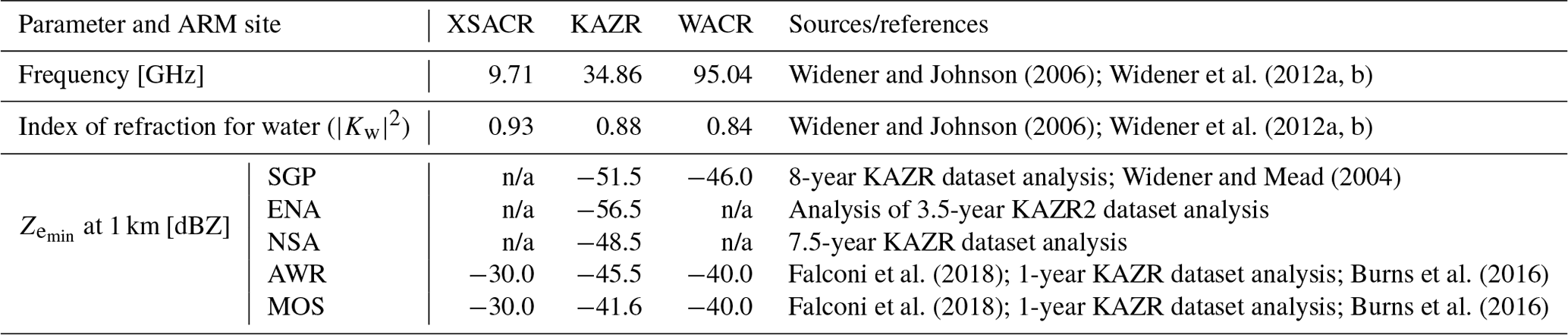
n/a – not applicable
EMC2 incorporates a suite of unit tests for each function using the pytest testing tool (https://pytext.readthedocs.io/, last access: 1 December 2021) to inspect the integrity and functionality of the code. These unit tests are combined with continuous code integration using TravisCI integration service (https://travis-ci.com/, last access: 1 December 2021), which runs the unit tests every time a developer submits a pull request on GitHub. If the unit test passes with the developer's changes to the code, then the changes are approved to be a part of EMC2. Documentation is also automatically generated from the metadata strings in each subroutine to ensure that each part of the code is well documented.
2.2 Allocation of hydrometeors to subcolumns
The following simulator description assumes large-scale model convective and/or stratiform cloud scheme outputs containing four hydrometeor classes: cloud water (cl), cloud ice (ci), rain (precipitating liquid; pl), and snow (precipitating ice; pi). While these four hydrometeor classes are widely used in various microphysics schemes, we note that EMC2 can be generally adapted to cases in which fewer or additional classes are used. We note that all the acronyms, abbreviations, and symbols used throughout this study are listed in Appendix A.
The subcolumn allocation and forward calculations in EMC2 can be performed using two main approaches; the first follows the assumptions and general logic implemented in large-scale model radiation schemes while the second follows the assumptions and logic in model microphysics schemes. In short, the radiation scheme approach largely treats hydrometeor fractions in a generalized manner and utilizes bulk (hydrometeor population) scattering lookup tables (LUTs) generated using specific size distribution assumptions. The microphysics scheme approach, on the other hand, includes full integration of single-particle scattering LUTs using hydrometeor particle size distributions prognosed by models with consideration of sub-grid hydrometeor class fraction variability assumptions.
We note that the detailed description below of the radiation and microphysics approaches is congruent with the current implementation of these approaches in the GISS ModelE3 climate model. However, the core of these approaches is similar in other climate and Earth system models (ESMs), and EMC2 can be easily adapted to fit specific variations in a model assumptions (see Sect. 2.1). For example, the microphysics approach currently operates only on stratiform microphysics scheme output using a two-moment bulk scheme (Gettelman and Morrison, 2015, hereafter MG2) that has been implemented in climate models such as the Community Earth System Model version 2 (CESM2) Community Atmosphere Model version 6 (CAM6) (Danabasoglu et al., 2020), the Energy Exascale Earth System Model (E3SM; Golaz et al., 2019), and ModelE3.
Prior to the radar and lidar forward calculations, EMC2 generates subcolumns for each model output column. These subcolumns emulate a higher model spatial resolution, which partially reconciles the locality of ground-based measurements and allows a more robust statistical model evaluation. Subcolumns are generated and populated with hydrometeors from the top-down using the maximum-random overlap approach (Tian and Curry, 1989; Fan et al., 2011; Hillman et al., 2018) similar to the description by Lamer (2019, chap. 6). EMC2 translates hydrometeor fractions in the model grid to a binary set of hydrometeor-containing and hydrometeor-free subcolumn bins. That is, given a specified number of subcolumns (Ns; determined by the user), the total number of hydrometeor-filled subcolumn bins at model level h and time step t is equal to the rounded value of , where fhyd is the volume fraction of a hydrometeor class (e.g., fcl, fpi) or a generalized hydrometeor fraction (fgen) used in the model radiation scheme, at the same model level and time step. Here and henceforth, we assume for simplicity an SCM output (no horizontal coordinate dimensions), even though EMC2 can generally operate not only on SCM simulation output but also on global simulation output. Note that EMC2 does not calculate fgen, but can use it if it is a model output field. The fgen parameter is a generalization of cloud and precipitation fractions denoting air volume in which scattering and absorption by hydrometeors influence radiative calculations for a model. (In the case of ModelE3, for example, fgen corresponds to cloud fraction where the layer-average cloud opacity exceeds that of precipitation, or vice versa.)
The following steps are applied in order to populate subcolumns (number ) with hydrometeors:
-
Convective cloud hydrometeors (cl and ci) are allocated to the first subcolumns (lowest index; if ), thereby generating cloud-containing subcolumns with maximum convective geometrical cloud depths.
-
Stratiform cloud hydrometeors are allocated to subcolumn bins unoccupied by convective cloud hydrometeors following the maximum-random overlap approach. Thus, stratiform clouds at model level h are first randomly allocated to subcolumn bins with overlying stratiform clouds (at level h+1), followed, if necessary, by random allocation to subcolumns with cloud-free bins directly above at level h+1. This order of processing where clouds are preferentially extended vertically conforms with assumptions that are often implemented in large-scale model radiative transfer calculations. (Note that our objective is to be faithful to model physics, even though in the case of the maximum-random overlap approach, it could produce, in certain cases, larger model biases compared to observations (e.g., Hillman et al., 2018).) During this hydrometeor allocation step, maximum overlap between liquid and ice cloud hydrometeors is maintained in grid cells containing both cloud phases. For example, if , all cl-containing subcolumn bins belonging to the same grid cell will necessarily contain ci as well (mixed-phase), but there will be additional subcolumn bins in that grid cell containing only ci hydrometeors. In the case where overlying stratiform hydrometeors exist, the overlying layer phase is not a factor of consideration, such that a subcolumn bin containing ci may be located right above a subcolumn bin containing cl or both cl and ci (mixed-phase), and vice versa.
-
Convective and stratiform precipitating hydrometeors (pl and pi) are allocated to subcolumns without convective-stratiform restrictions, such that convective and stratiform precipitation may co-exist in the same subcolumn bin. Similar to the stratiform cloud allocation, precipitation is allocated with maximum-random overlap; i.e., precipitation is first extended vertically. Thus, either stratiform or convective cloud hydrometeors may exist in the same subcolumn bins as convective and/or stratiform precipitating hydrometeors (for example, describing a scenario of snow generated by a stratiform cloud seeding an underlying drizzling stratocumulus cloud field). If after the vertical extension of overlying precipitation some subcolumn bins are still to be populated with precipitating hydrometeors (e.g., in a case where and ), these hydrometeors are randomly allocated to cloudy grid cells of the same type (convective or stratiform), followed by random allocation of hydrometeors to cloud-free subcolumn bins. Similar to the allocation of stratiform cloud hydrometeors, maximum overlap is maintained between liquid and ice precipitation, and overlying precipitation phase is not a factor of consideration during the step of vertical extension of precipitation.
Once the subcolumns are populated with hydrometeors, per hydrometeor class except for stratiform cl in the case of the microphysics approach, hydrometeor mixing ratio is set in every hydrometeor-containing subcolumn bin by , where qhyd and designate the mixing ratio of a hydrometeor class (e.g., qcl, qci) in subcolumn bin s and a corresponding model grid cell mean, respectively. In the case of cl when using the microphysics approach, at every model level h and time step t, is randomly set in cl-containing subcolumn bins such that it would comply with the sub-grid variability gamma distribution described by Morrison and Gettelman (2008, Eq. 8) while adjusting the values in the last cl-containing subcolumn bin such that hydrometeor mass is conserved (as in the case of other hydrometeor classes), i.e.,
We note that sub-grid scale variability of cloud water in ModelE3 is tied to the sub-grid scale variability of moisture rather than set at a fixed value as in Morrison and Gettelman (2008).
In stratiform hydrometeor-containing subcolumn bins, hydrometeor number concentration is set for every hydrometeor class by , where Nhyd and designate the number concentration of a hydrometeor class in subcolumn bin s and a corresponding model grid cell, respectively. EMC2 assumes that convective schemes do not diagnose , and hence, this information is currently not produced by the simulator.
2.3 Forward calculation of lidar variables
2.3.1 Microphysics approach
In the microphysics approach, applicable only to stratiform hydrometeors, per hydrometeor diameter D, EMC2 calculates the hydrometeor size distribution, , defined by qhyd and Nhyd, fully consistent with the MG2 scheme (see Morrison et al., 2009, Eqs. 1–3). Using LUTs containing full Mie calculations for spheres (following Bohren and Huffman, 1983, Appendix A) of single particle extinction and backscatter efficiencies at lidar operating wavelength λl ( and , respectively), the lidar particulate extinction cross-section () and backscatter cross-section () are calculated in every hydrometeor-bearing subcolumn bin by
where we use the trapezoidal rule for discrete integration over a series of D values, which can be unevenly spaced by , while noting that and , where ND is the number of diameters for which , , and ϕhyd are calculated. In the case of the Mie calculations currently available in EMC2, D1=0.1 µm, cm, and is constant and equals 0.1 µm. The complex refractive indices (mhyd(λl)) used for liquid hydrometeors in the Mie calculations can be taken from Segelstein (1981, Table 1) or Rowe et al. (2020, for a temperature of −10 ∘C). Refractive indices for ice hydrometeors are taken from Warren and Brandt (2008). The Maxwell Garnett equation (Bohren and Battan, 1980, Eq. 1) for a mixture of ice and air is used to calculate the effective mhyd for ci and pi based on the ice densities implemented in EMC2 for ModelE3 (Table 1) relative to bulk ice density of 917 kg m−3.
The total αp and βp ( and , respectively) are calculated as the sum of each of these variables for cl, ci, pl, and pi. The lidar linear depolarization ratio (LDR) is estimated by weighting fixed LDR values (per hydrometeor class; see Table 1) with the relative contribution of to .
The cumulative optical thickness (from the surface upward) at the base of a given subcolumn bin, τhyd, is calculated by
where Δz(h,t) denotes the geometrical thickness of model level h at time step t and . The total integrated optical thickness, , being the sum of τhyd for cl, ci, pl, and pi, is used to estimate the level of full lidar signal attenuation (received signal not detectable by the simulated instrument), the value of which can be used to constrain comparisons between model output forward calculations and observations. Lidar signal extinction at visible wavelengths typically occurs at an optical thickness of 3–5 (e.g., Sokolowsky et al., 2020, Fig. 4), and hence, EMC2 assumes by default that the lidar signal is extinct at a level where τtot=4 to produce a lidar signal extinction mask. We note that EMC2 allows calculating τhyd from the top-down (i.e., at the top of a given model layer), thereby enabling simulation of airborne and spaceborne lidar measurements.
In some cases, the observational dataset only consists of measurements made by elastic lidars that do not allow direct retrieval of αp and βp. In these cases, observations can be compared with a diagnostic attenuated , , which is often referred to as the normalized relative backscatter (NRB; Campbell et al., 2002) after several lidar signal corrections are applied. is calculated here by
where βm and are the molecular backscatter cross-section and the two-way transmittance calculated following Penndorf (1957), and η is the multiple scattering coefficient. The value of η is set to 1 by default, effectively implying no multiple scattering by hydrometeors or perfect multiple scattering treatment. Such an assumption is not realistic in the vast majority of cases even though effective η values closer to 1 are more likely given the common narrow field-of-view of ground-based (and airborne) lidars. While a value of 1 is most likely unrealistic, it precludes the introduction of additional confounding factors stemming from the dependence of multiple scattering effects on the hydrometeor particle size distributions (e.g., Eloranta, 1998), which could significantly impact model–observation comparisons of (not shown). Moreover, this dependence of multiple scattering on particle size distributions suggests that a fixed η value smaller than 1 would impact the faithfulness of the lidar simulator to the model physics. That said, we note that η can be manually set to other fixed values based on the physical assumptions made or certain empirical results (e.g., Winker, 2003), and that the determination of the extinction level based on τtot is independent of η.
2.3.2 Radiation approach
With the radiation approach, applicable to both stratiform and convective cloud scheme output, forward calculations rely on bulk scattering LUTs. Therefore, this approach is more than 2 orders of magnitude faster than the microphysics approach, thereby rendering EMC2 more suitable for the analysis of large model output datasets. Using this approach, a geometric cross-sectional area for each hydrometeor-bearing subcolumn bin is first calculated assuming geometric scatterers:
where ρa is the density of air, ρb is the bulk density of the hydrometeor class phase (1000 and 917 kg m−3 is the case of liquid and solid water, respectively), and is the effective radius of a hydrometeor class in the model grid cell, provided as a model output field. The and are then calculated by
where and represent in this case bulk efficiencies per unit volume taken from LUTs, in which they are provided as function of . In Eqs. (6a) and (6b), however, and are functions of the adjusted effective radius, , which equals in all hydrometeor classes and cloud types except for stratiform cloud ice and snow. In these two cases, and , where ρhyd is the hydrometeor class density (see Table 1), and Φhyd is a constant fluffiness factor. Φhyd is used such that a value of 0 represents an equivalent mass bulk sphere while a value of 1 represents a fluffy sphere with an equivalent maximum dimension as in Gettelman and Morrison (2015). In the case of ModelE3, for example, Φhyd is set by default to an intermediate value of 0.5 and generally serves as one of many tuning parameters
The default and in Eqs. (6a) and (6b) (respectively) implemented in EMC2 were calculated using single-particle full Mie calculations in the case of liquid hydrometeors and single-particle scattering LUTs for a severely roughened eight-column ice aggregate (Yang et al., 2013) in the case of solid hydrometeors. These ice aggregate scattering calculations have been shown by Holz et al. (2016) to enable a closure between infrared Moderate-Resolution Imaging Spectroradiometer (MODIS; Platnick et al., 2003) and visible Cloud-Aerosol Lidar with Orthogonal Polarization (CALIOP; Winker et al., 2009) satellite ice optical thickness retrievals and were included in the MODIS collection 6 (C6) cloud product (Platnick et al., 2017). In order to calculate the and LUTs, we assumed the same gamma distribution parameters as those implemented in the C6 dataset (see Hansen, 1971, Eq. 1), consistent with the bulk LUTs utilized by ModelE3's radiation scheme.
Following the calculations of and , the total variables and as well as τhyd, τtot, and are calculated as in the microphysics approach (Sect. 2.3.1).
2.4 Forward calculation of radar variables
2.4.1 Microphysics approach
When the microphysics approach is selected in EMC2, the first three radar moments are calculated for each hydrometeor class in every hydrometeor-bearing subcolumn bin, that is, the equivalent reflectivity factor (), the mean Doppler velocity () and the Doppler spectral width () as well as total radar moment variables (, , and ). Full Mie calculation LUTs for the emulated radars (Table 2) are first used to calculate at the radar operating wavelength λr following Eq. (2b). The mhyd(λr) used for liquid in the Mie calculations can be taken from Segelstein (1981, Table 1) or Turner et al. (2016, using a temperature of −10 ∘C), while mhyd(λr) values for ice are taken from Mätzler (2006, chap. 5.3; using temperature of −10 ∘C). in every hydrometeor-containing subcolumn bin is then calculated (in linear units) using (Doviak and Zrnić, 1993, Eq. 4.33)
where is the dielectric factor for water used in the raw radar observational processing (see Table 2). Using the resultant , is then calculated by implementing the hydrometeor class terminal velocities parametrization used in the MG2 scheme (cf. Morrison and Gettelman, 2008, Table 2). In the calculation of we neglect the model grid cell vertical wind, w, which predominantly has little impact on the value, especially at coarser spatial and temporal resolutions typical to large-scale models. Finally, is calculated, while we note that beamwidth and turbulent broadening (e.g., Chen et al., 2018) are omitted from this calculation but will be added in future work.
To allow a valid comparison between the forward calculations and observations, signal attenuation is considered in the calculation of the attenuated , :
where Ygas and are the one-way integrated attenuation at the base of the subcolumn bin (in dB) due to atmospheric gases (O2 and H2O; see Ulaby et al., 1981, Sect. 5.3–5.5) and all hydrometeors, respectively. is calculated using
where is determined by summing based on Eq. (2a) calculated at λr over all hydrometeor classes while setting .
The vertical profile of the minimum detectable equivalent reflectivity factor, , is calculated by
where z(h,t) is the height at the base of model level h (in meters) at time step t and is the minimum detectable signal at 1 km (using the highest sensitivity mode; Table 2). When compared with observations, subcolumn bins where can be treated as returned signal below the radar noise floor and, hence, are effectively considered hydrometeor-free.
2.4.2 Radiation approach
When the radiation approach is selected in EMC2, forward radar calculations using bulk LUTs are limited to the zeroth radar moment (Ze) due to a set of limitations:
-
Large-scale model radiation schemes are not informed with hydrometeor fall velocities. Moreover, fall velocity parametrizations in microphysics schemes do not necessarily fully overlap with the hydrometeor size and shape assumptions implemented in radiation schemes.
-
Noting that EMC2 operates off-line, hydrometeor class fall velocities are typically reported in model outputs as weighted means. Because not all cloud schemes enable back-tracing of hydrometeor class fall velocities as a function of particle diameter using analytical expressions and weighted output fields (e.g., the convective cloud scheme in ModelE3; see Elsaesser et al., 2017), hydrometeor class fall velocities per subcolumn bin cannot be straightforwardly reproduced.
-
The total radar moments include combinations of the different hydrometeor class mixing ratios and, hence, cannot be determined using a single set of bulk LUTs per hydrometeor class.
Thus, EMC2 calculates only the , , and . Equations (6b) and (7) are used to calculate with bulk scattering LUTs for λr based on full single-particle Mie scattering calculations in the case of liquid hydrometeors and single-particle scattering calculations for the Yang et al. (2013) eight-column aggregate at a temperature of 270 K (see Ding et al., 2017) in the case of solid hydrometeors. Similar to the implementation of the radiation approach in the forward lidar calculations (Sect. 2.3.2), considers the fluffiness factor in the case of solid (ice) hydrometeors. Finally, and are calculated similar to the microphysics approach using Eqs. (8) and (9) with (and ) calculated using Eq. (6a).
2.5 Hydrometeor classifications
Once the total lidar and/or radar variables are calculated, EMC2 can be used to classify the subcolumn simulator output. Classification masks can serve as tools for direct comparisons between the simulator output and observational data utilizing similar classification methodologies, some of which can be used to calculate water phase ratios. Currently, EMC2 incorporates three hydrometeor classification methods: the radar-sounding cloud and precipitation detection and classification, the modified fixed lidar variable threshold phase classification, and the COSP lidar simulator emulator (henceforth referred to as the COSP emulator; “emulator” is used here in its generic sense rather than a machine-learning context, and there is no training involved).
The radar-sounding cloud and precipitation detection method (Silber et al., 2021a; see also Vassel et al., 2019) emulates the combined use of relative humidity with respect to water (RH) sounding measurements for the detection of liquid-bearing clouds and radar echoes (received signal above the radar noise floor) for the detection of precipitating hydrometeors. In the case of large-scale model output, RH below 100 % in a model grid cell does not necessarily indicate a lack of cloud water, because of implemented assumptions concerning the sub-grid distribution of cloud water content (e.g., Smith, 1990). Therefore, the approach most consistent with the observational method is to simply use the cloud water-bearing subcolumn bins (see Sect. 2.2) to classify the subcolumn bin as “cloud”. “Precipitation” are those subcolumns bins in which . Subcolumn bins that can be classified as both “cloud” and “precipitation” are set as “mixed”. We note that at temperatures below 0 ∘C, the “mixed” classification type becomes more likely to represent a mixed-phase cloud with decreasing temperatures but, in general, may represent bins containing only liquid hydrometeors.
The modified fixed lidar variable threshold phase classification method is similar to previous studies that incorporated fixed LDR and thresholds to classify hydrometeor-bearing air volumes to “liquid” and “ice-only” using lidar measurements (e.g., Shupe, 2007; Thorsen and Fu, 2015). By default, however, EMC2 includes two additional “undefined” classes that cover intermediate regions in the LDR-, such that a subcolumn bin classified as “undefined1” has a higher probability that it includes some amount of liquid water while “undefined2” is more likely to only contain ice hydrometers (see Sect. 3.3 for discussion and illustration of the default thresholds). The notion behind the addition of these two “undefined” classes is the fixed-threshold method limitations that could originate in the following:
-
Drizzle- or rain-bearing air volumes may produce moderate and LDR on the order of 0.1, especially when ice hydrometeors are present in the same air volumes (e.g., Derr et al., 1976; Sassen, 2003; Silber et al., 2019a).
-
Cases can occur in which an entire relatively tenuous liquid-bearing cloud layer or other cases with liquid-bearing air volumes just above cloud base occur concurrently with ice precipitation sufficiently concentrated and intense to generate a combination of high and LDR that can reach values of 0.10–0.20 (e.g., Derr et al., 1976; Silber et al., 2018b, Fig. S1). This influence of ice hydrometeors also applies to rain-bearing air volumes.
-
Horizontally oriented ice hydrometeors may produce low (moderate) LDR () via specular reflection even in cases when the lidar is titled up to several degrees off-zenith (e.g., Noel et al., 2002; Silber et al., 2018b, Appendix A). Note that this limitation only applies to observations, since specular reflection and ice particle canting angles are not represented in large-scale models.
Adaptive fixed thresholds that vary with site, instrument, and period of study (e.g., Silber et al., 2018a; Zaremba et al., 2020) or lidar ratio constraints (e.g., Thorsen and Fu, 2015) can compensate for some of these limitations. However, these approaches cannot be objectively translated to the model output domain to enable a direct comparison between the observations and the simulator output. Therefore, the modified fixed threshold routine, which largely agrees with existing measurements yet acknowledges both model and observational uncertainties, may allow better direct comparisons to be made.
The emulator of the COSP lidar simulator follows the same equations and logic of the on-line lidar simulator (Cesana and Chepfer, 2013) implemented in numerous climate models. In short, the attenuated total backscatter (ATB) calculated in the COSP emulator routine while assuming η=0.7 is used to calculate the lidar scattering ratio (the ratio of total to molecular attenuated backscatter) for the detection of hydrometeors in subcolumns by selecting scattering ratio values larger than 5. Calculated cross-polar ATB as a function of the total ATB is then used to classify the detected hydrometeors into liquid or ice, based on an empirical phase discrimination line. As the last step of this classification method, hydrometeors below (top-down lidar view) or above (bottom-up lidar view) a subcolumn bin with scattering ratio larger than 30 are classified as “undefined”. Note that, unlike the on-line COSP lidar simulator, this emulator operates using the model vertical levels and does not interpolate the model output onto an evenly spaced vertical grid. As with all other EMC2 forward calculations and classification routines, this emulator can operate using a top-down viewing approach thus providing a bridge between the COSP simulator and EMC2.
Finally, EMC2 also includes internal functions to calculate mass or frequency phase ratios using each of these hydrometeor classification methods, providing metrics to compare model output with observations or with outputs from other models.
To demonstrate the application of EMC2 and its output using the different forward calculation approaches, here we describe and analyze a Lagrangian LES case study (Silber et al., 2019a) adjusted for running and testing the ModelE3 climate model (as well as other climate models) in SCM mode.
3.1 Case description
As described by Silber et al. (2019a), the stratiform cloud event that we compare with model simulations was observed over McMurdo Station, Antarctica, as part of the ARM West Antarctic Radiation Experiment (AWARE; Lubin et al., 2020), on 16 August 2016. During the event, cyclone-driven wind confluence with southwesterly katabatic flow resulted in relatively warm and moist marine air convergence along the Ross Ice Shelf coast, part of which was advected towards the McMurdo Station measurement site (Fig. 2a). This air convergence induced a widespread (>1000 km) cloud field evident by Clouds and the Earth’s Radiant Energy System (CERES) measurements indicating an extensive region with enhanced top of atmosphere (TOA) upwelling longwave radiation (dashed green shape in Fig. 2b; note that a surface-based temperature inversion is common during the austral winter resulting in smaller TOA radiation fluxes).
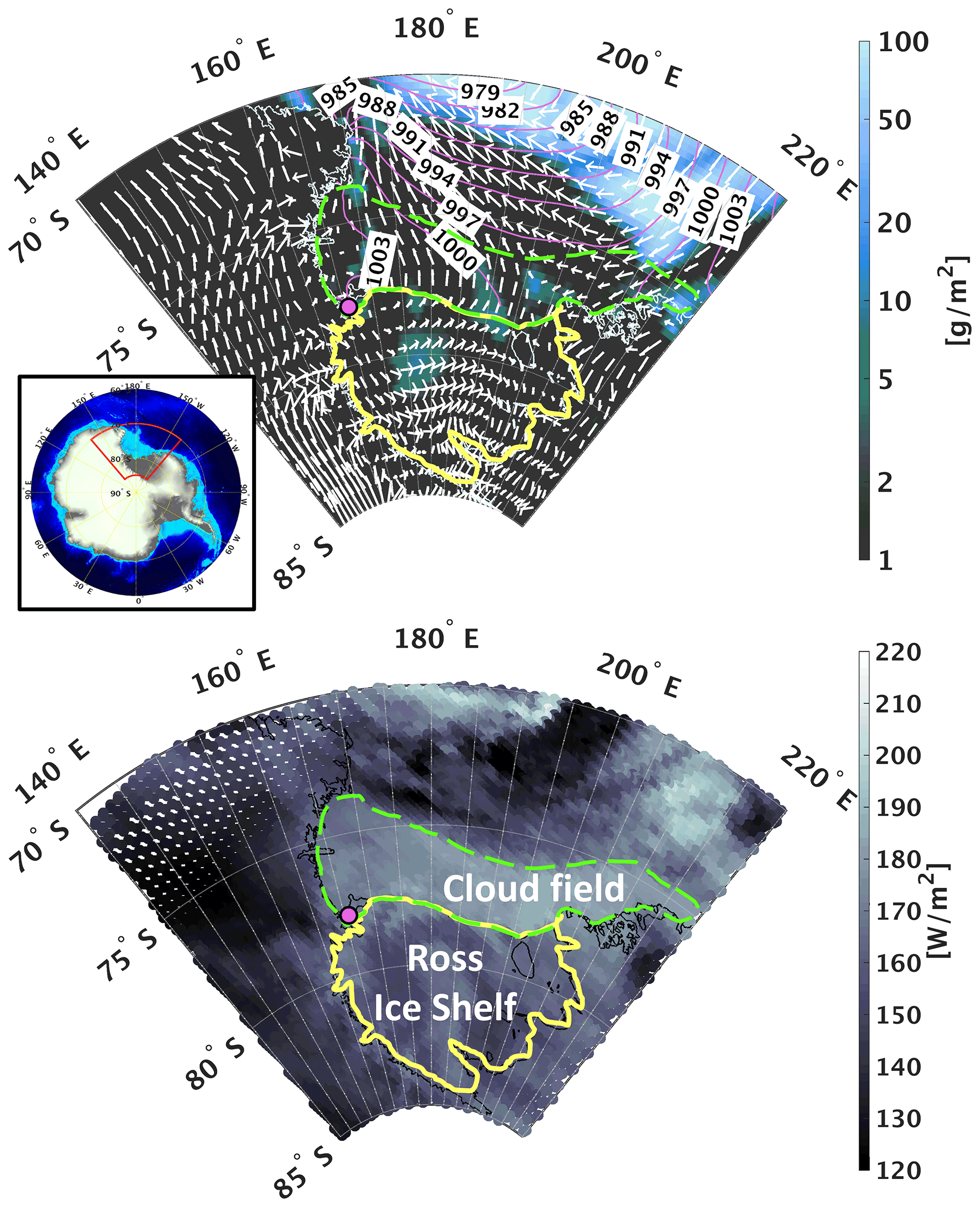
Figure 2(Top) Sea level pressure (contours; land areas are masked), total condensate water path (logarithmic color scale), and surface winds (quivers) resolved by ERA5 (Hersbach et al., 2020) for 16 August 2016, at 10:00–11:00 UTC. The magenta-filled marker denotes McMurdo Station. The dashed green shape highlights a widespread cloud field along the Ross Ice Shelf (yellow shape) coast associated with the ground-based observations. The inset panel shows a topographic map of Antarctica (the red box highlights the region depicted in the main panel). (Bottom) Top of atmosphere upwelling longwave radiation measured by CERES Aqua on 16 August 2016, at 10:44–10:50 UTC. The 1 arcmin topographic data were developed by the National Geophysical Data Center (NGDC Amante, 2009) and are freely available at https://www.ngdc.noaa.gov/mgg/global/global.html (last access: 1 December 2021). Reproduced from Silber et al. (2019a).
Over McMurdo Station, a decoupled persistent mixed-phase cloud with temperatures as low as −29 ∘C was observed for ∼ 39 h. The observed cloud was nearly continuously precipitating ice particles and was also drizzling for more than 7 h, concluded from a comprehensive analysis of sounding, HSRL, and KAZR measurements (see Silber et al., 2019a).
3.2 ModelE3 SCM configuration
Based on Lagrangian simulations constrained by the remote-sensing observations, Silber et al. (2019a) postulated that the activated ice-nucleating particle (INP) and cloud condensation nuclei (CCN) concentrations during the event were on the order of 0.2 L−1 and 20 cm−3, respectively, to enable drizzle to be produced and precipitate along with ice precipitation below the highly supercooled cloud base. Their simulations were 9 h in duration, starting on 16 August 2016, at 01:00 UTC and ending at 10:00 UTC. By imposing large-scale vertical wind extracted from back-trajectory calculations, they emulated the transport of the cloud layer, initially forming in a stable layer, towards McMurdo Station. The end of the simulation at 10:00 UTC designated the time at which the cloud field reached the fixed observational site at McMurdo, and hence, statistics of that hour of observations (10:00–11:00 UTC) were compared with the model output.
Here, we slightly adjusted the case study initialization files to enable running this case in a climate model's SCM mode while using the same single hour of radar and lidar observations and the Distributed Hydrodynamic Aerosol and Radiative Modeling Application (DHARMA) model (Stevens et al., 2002) baseline LES output (see Silber et al., 2019a) as benchmarks. Namely, we simplified the profiles of vertical motion (as in Silber et al., 2020) and then converted the height coordinates of the initial sounding (see Silber et al., 2019a) and vertical wind time series to pressure coordinates (these converted sounding and forcing files are available at https://doi.org/10.17632/gz4gdn3jvz.1, Silber, 2021). The utilization of these files to run the highly supercooled cloud case study enables testing of an SCM and, hence, the cloud schemes implemented in a climate model.
The LES is initialized here with activated INP concentration of 0.1 L−1 and with both cloud ice and snow hydrometeor classes (whereas Silber et al. (2019a) used only a single ice class), and the simplified vertical motion profiles are then imposed. These few LES adjustments make the model configuration more consistent with climate model microphysics and SCM initialization while effectively resulting in the same hydrometeor content and cloud evolution as the baseline simulation presented in Silber et al. (2019a) (not shown). Thus, the SCM is run equivalently to the LES, that is, using the same initial sounding and forcing files, setting the coordinates to −77.85∘ S, 166.72∘ E, and prescribing a monomodal log-normal aerosol particle concentration of 20 cm−3 with a mean radius of 0.1 µm, geometrical standard deviation of 2, and a hygroscopicity parameter of 0.4. We note that activated INP concentrations are not prescribed in the SCM simulations because (a) ModelE3's final configurations are defined by specific values of certain model tuning parameters (among others) associated with INP parameterization, and (b) diagnostically prescribing the activated INP concentration is not faithful to the temperature-dependent approach implemented in the model and, hence, would not necessarily be informative of true climate model weaknesses.
3.3 Comparison between observations and ModelE3 SCM using EMC2
The following figures show the EMC2 forward calculation results using the DHARMA LES simulation and ModelE3's configuration Tun3, one of four configurations of ModelE3 derived in part via a machine learning parameter tuning approach that will be described in a manuscript in preparation, to be included in the Coupled Model Intercomparison Project Phase 6 (CMIP6). The SCM using this configuration was able to generate a cloud-top inversion and turbulent layer via cloud-top radiative cooling and produced the best agreement with the observations and the LES relative to the other three configurations (see Appendix B). Whereas here we examine application of EMC2 to a single ModelE3 configuration in SCM mode in a case where we can also compare with LES, we note that EMC2 is designed to enable detailed evaluation of atmospheric thermodynamic profile and cloud properties extracted from global simulations of ModelE3 configurations and other climate models against long-term datasets at fixed sites in future dedicated work.
The left panels in Fig. 3 show the mixing ratios of the four hydrometeor classes evolving through the simulated SCM case study. These depicted mixing ratios are the output of the SCM's stratiform cloud scheme, but because this simulation does not generate any convective hydrometeors (as expected), they also represent the total mixing ratios. Cloud water mass (top panel) dominates over the other hydrometeor classes in hydrometeor-bearing model grid cells through much of the simulation, even at lower levels in which the cloud water fraction is rather low (Fig. 3, right panels). Rain (effectively drizzle) is produced by the model as well but has a relatively smaller mass compared with that of snow generated. This reduced amount of rainwater in the SCM simulation relative to rainwater dominance in the simulations of Silber et al. (2019a) is largely the result of the different autoconversion parameterization schemes implemented in ModelE3 (Seifert and Beheng, 2001) relative to that implemented by default in the DHARMA LES (Khairoutdinov and Kogan, 2000), which produces significantly smaller rain mass mixing ratios in this case (not shown), contrary to some previous studies (e.g., Heiblum et al., 2016; Xiao et al., 2021). Understanding the source of this differing autoconversion parameterization behavior requires a dedicated study that is a beyond the scope of this article.
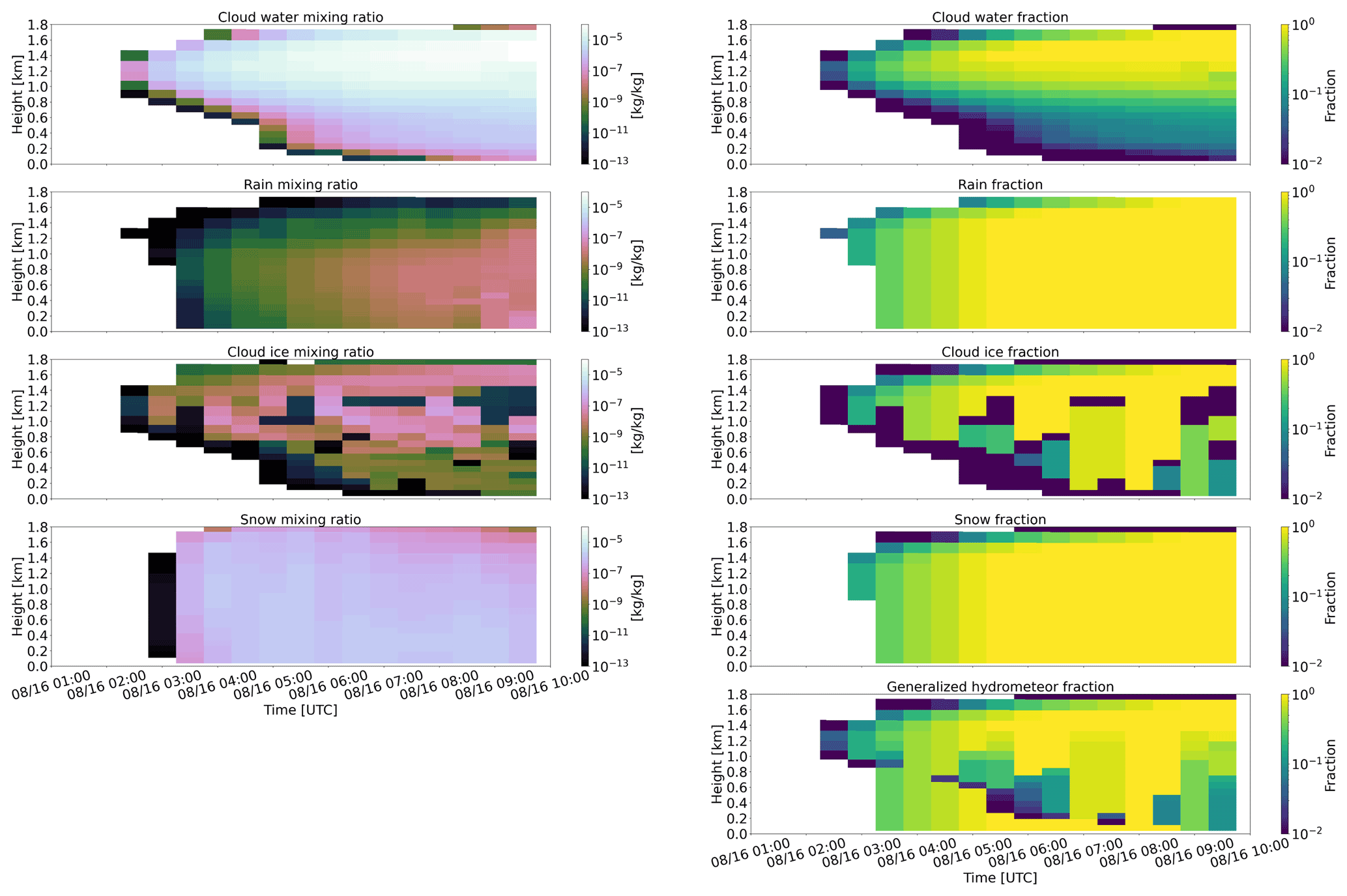
Figure 3ModelE3 configuration Tun3 single-column model (SCM) output for the Antarctic cloud case study (16 August 2016) showing mixing ratio (left) and hydrometeor fraction (right) time–height curtain plots of (from top to bottom) cloud water, rain, cloud ice, and snow. The generalized hydrometeor fraction used in the radiation approach (see Sect. 2) is depicted in the bottom right panel.
Figures 4 and 5 depict the HSRL and KAZR variables observed during a single hour over McMurdo Station and simulated with EMC2 using the DHARMA LES three-dimensional output at the end of that simulation (without using the subcolumn generator), and by applying each of the three approaches on ModelE3 configuration Tun3 SCM output for 05:00 UTC. Because our goal in this section is to demonstrate that EMC2 can reasonably match cloud observations given comparable input, we present the EMC2-processed SCM output 4 h into the simulation when cloud top heights are similar to observed instead of the end of the simulation (the SCM develops the supercooled cloud faster than the baseline LES; see Appendix B). When evaluating the processed model output against the observations, we essentially exchange temporal resolution with spatial resolution (three-dimensional model domain in the case of the LES) or an emulated spatial resolution (in the case of the SCM). We set the number of SCM subcolumns (Ns) to 100, which effectively represents hydrometeor class fractions up to the second decimal point and enables drawing more robust statistics by emulating sub-grid variability of all hydrometeor classes combined.
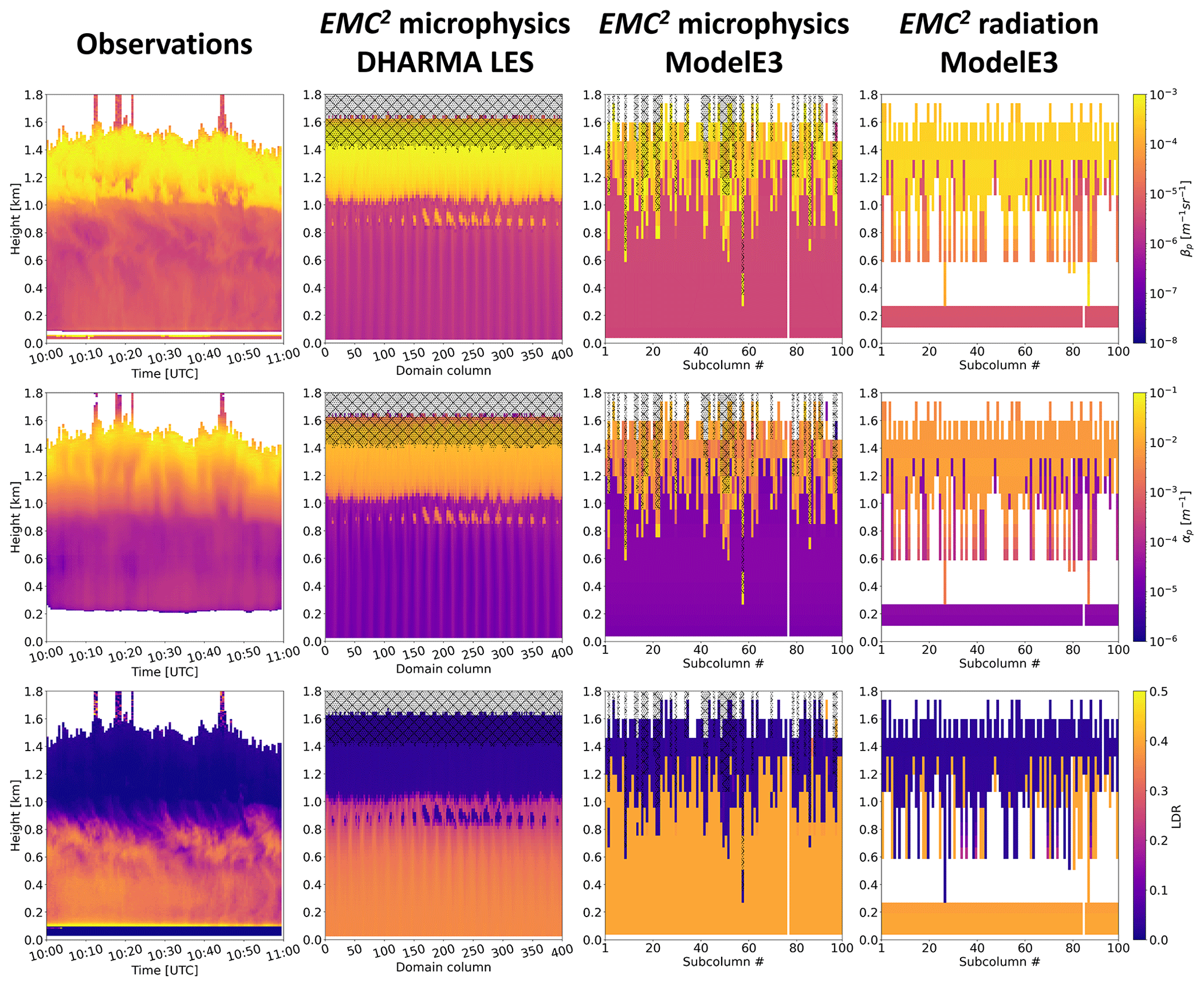
Figure 4Observed and simulated HSRL particulate backscatter cross-section (; top row), particulate extinction cross-section (; middle row), and linear depolarization ratio (LDR; bottom row) using the DHARMA LES output and ModelE3 configuration Tun3 SCM output. The columns show (from left to right) the observations from McMurdo Station between 10:00–11:00 UTC, DHARMA LES three-dimensional output (horizontal dimensions stacked onto a single domain column dimension) processed using EMC2 microphysics with the subcolumn generator turned off (Ns=1), ModelE3 EMC2 output using the microphysics approach, and EMC2 output using the radiation approach. The DHARMA LES output corresponds to 10:00 UTC (arrival of cloud field at McMurdo Station; see Sect. 3.2), while ModelE3's EMC2 panels depict the SCM output for 05:00 UTC (see text) processed with EMC2 using 100 subcolumns. A mask denoting full lidar signal attenuation generated using a total accumulated optical thickness (τtot) condition of τtot>4 is plotted over the simulated data (hatched areas).
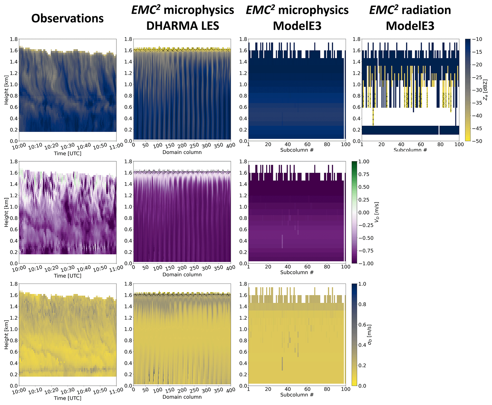
Figure 5As in Fig. 4, but with the KAZR attenuated equivalent reflectivity factor (; top row), mean Doppler velocity (; middle row), and spectrum width (; bottom row). Note that only is calculated in EMC2's radiation approach (see Sect. 2.4.2). A radar signal-to-noise ratio (SNR) mask of ( is the minimum detectable signal on each model level) is applied to the plotted data (hatched areas).
The processed LES output exhibits good apparent agreement with the observations, evident by the comparable lidar and radar variable values and their horizontal variability (Figs. 4 and 5), the vertical cloud structure and boundaries, as well as the full lidar signal attenuation near cloud top (Fig. 4). A multi-layer cloud water structure developed by the LES is suggested by the intermittent breaks in the large and values, supported by a separate analysis of and (not shown). This multi-layer structure is also indicated by the lidar observations (Fig. 4) and was comprehensively discussed by Silber et al. (2019a).
Using the microphysics approach, the SCM sub-grid variability is more pronounced relative to the radiation approach owing to the implementation of cloud water sub-grid variability (as defined in the MG2 microphysics scheme), which is not considered in the radiation approach. Evaluation of heights with full cloud cover, indicated by the large and values (see also Fig. 3, right), suggests that the SCM has an apparent reasonable agreement with the observations there. ModelE3's macrophysics scheme leads to notably ragged liquid cloud base heights that are evident in the SCM fields compared to the more uniform liquid cloud base in both observations and LES, as discussed further below. Relatively enhanced values are produced in some SCM subcolumns, which leads to full lidar signal attenuation, as also indicated by the HSRL measurements (Fig. 4). Full lidar signal attenuation does not occur in this case using the radiation approach because of the uniform distribution of cloud water between subcolumns commensurate with τtot values just below the full attenuation threshold of 4 (not shown). The subcolumns with full lidar signal attenuation in the microphysics approach call for the use of radar measurements for cloud-top detection (e.g., Fig. 5 discussed below).
Except for the overestimated LDR values below the supercooled cloud layer relative to the observations, the values of the other two lidar variables and the general scenario structure appear to agree with the observations and LES in both the microphysics and radiation approaches, which exhibit an encouraging consistency with each other (Fig. 4). The comparison of the subcolumn-averaged lidar-variable profiles illustrated in Fig. 6 allows a more quantitative comparison. This figure better indicates that the DHARMA LES within the main liquid-bearing cloud layer is within the range of the observations and their uncertainty, consistent with the conclusions of Silber et al. (2019a) that activated CCN number concentrations were low during this highly supercooled drizzle event.
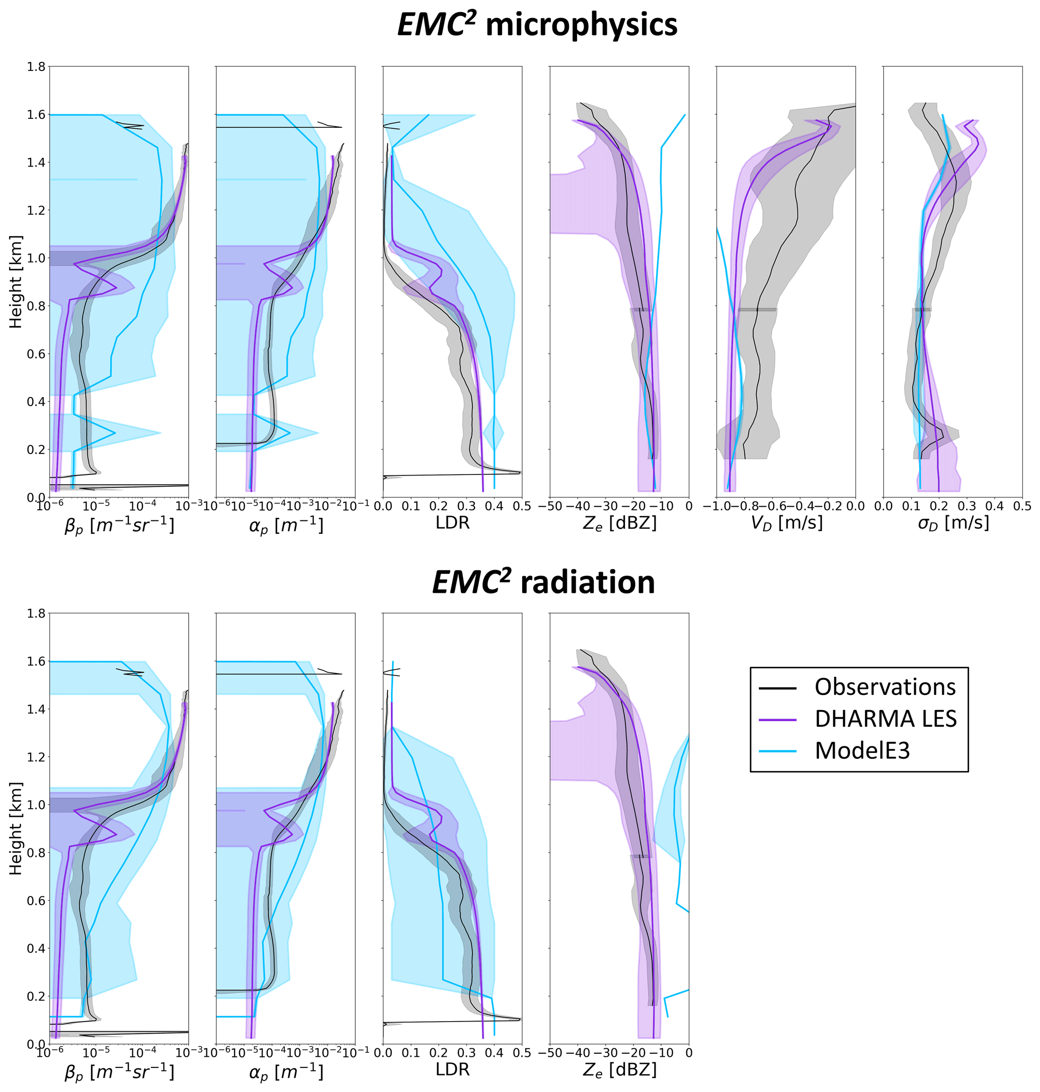
Figure 6Mean profiles of observed (time-averaged) and simulated (subcolumn-averaged) HSRL and KAZR variables calculated using EMC2's microphysics (top) and radiation (bottom) approaches as shown in Figs. 4 and 5 (full lidar signal attenuation and radar SNR masks are applied prior to averaging). Shaded regions denote the mean ±1 standard deviation.
The EMC2 lidar output also highlights a few model weaknesses. For example, using the microphysics approach, cloud base (at a height of ∼ 1.0 km) is highly variable and may extend nearly down to the surface, which is in contradiction to the observations, where cloud base variability is on the order of a few hundred meters throughout the depicted period (Fig. 4). Using the radiation approach, on the other hand, breaks in hydrometeor cover are seen below the fully overcast layer, as a result of the generalized hydrometeor fraction used in the radiative transfer calculations, which can be lower or higher than the associated hydrometeor class fraction (e.g., Fig. 3, right). Lesser (greater) generalized hydrometeor fractions relative to the associated hydrometeor class fraction therefore imply greater (smaller) subcolumn bin mixing ratios (see Eq. 1) and, hence, enhanced (diminished) associated and values. Thus, while the occurrence of low-level cloud water-bearing bins produces full attenuation of the simulated lidar signal in some subcolumns using the microphysics approach (Fig. 4), the smaller ensuing from the larger low-level generalized cloud fraction relative to the cloud water fraction (see Fig. 3, right) causes no low-level (or any level in this case) signal extinction when the radiation approach is used (see Fig. 4). Note that in both the microphysics and radiation approaches the subcolumn representation of hydrometeor mass remains consistent with the model output variables; i.e., Eq. (1) holds for each hydrometeor class.
The microphysics and radiation approaches exhibit values that are too large, especially at higher levels (Figs. 5 and 6). EMC2's radar processing using the microphysics approach provides the and variables in addition to the variable. We note that because spectral broadening terms other than the microphysical broadening are currently not considered in EMC2, the calculated generally serves as a lower bound for comparison purposes; i.e., the simulated values need to be smaller to some extent than the observed values. As indicated from Fig. 5, both and show grossly reasonable correspondence between the observations and the SCM, except at heights above ∼ 0.8 km, where values show large deviations (Fig. 6). A separate analysis (not shown) suggests that, in this case, these deviations are mainly the result of relatively fast fall velocities (see Table 1) and the dominance of large snow hydrometeors over at these levels and not the product of vertical air motion being convolved into the radar moments only in the observations.
Figure 7 delineates the three hydrometeor classification methods currently implemented in EMC2 applied over the processed model output, with the COSP emulator “observing” the model domain from the top down, similar to the on-line simulator. Congruent with the description above of the calculated radar and lidar variables, the radar-sounding and modified fixed lidar threshold methods show the domination of liquid hydrometeor classes above ∼ 1.0 km, the prevalence of precipitating hydrometeors at lower levels (with lower occurrence using the radiation scheme approach), and the occasional full attenuation of the simulated lidar signal in the case of the lidar-based classification method. The COSP emulator detects a clear liquid-bearing subcolumn bin signal at cloud tops. However, because the cloud-top layer is highly reflective, generating large lidar scattering ratio values (the ratio of total to molecular attenuated backscatter), most of the underlying layers are either classified as “undefined” or generate signals too weak to be detected.
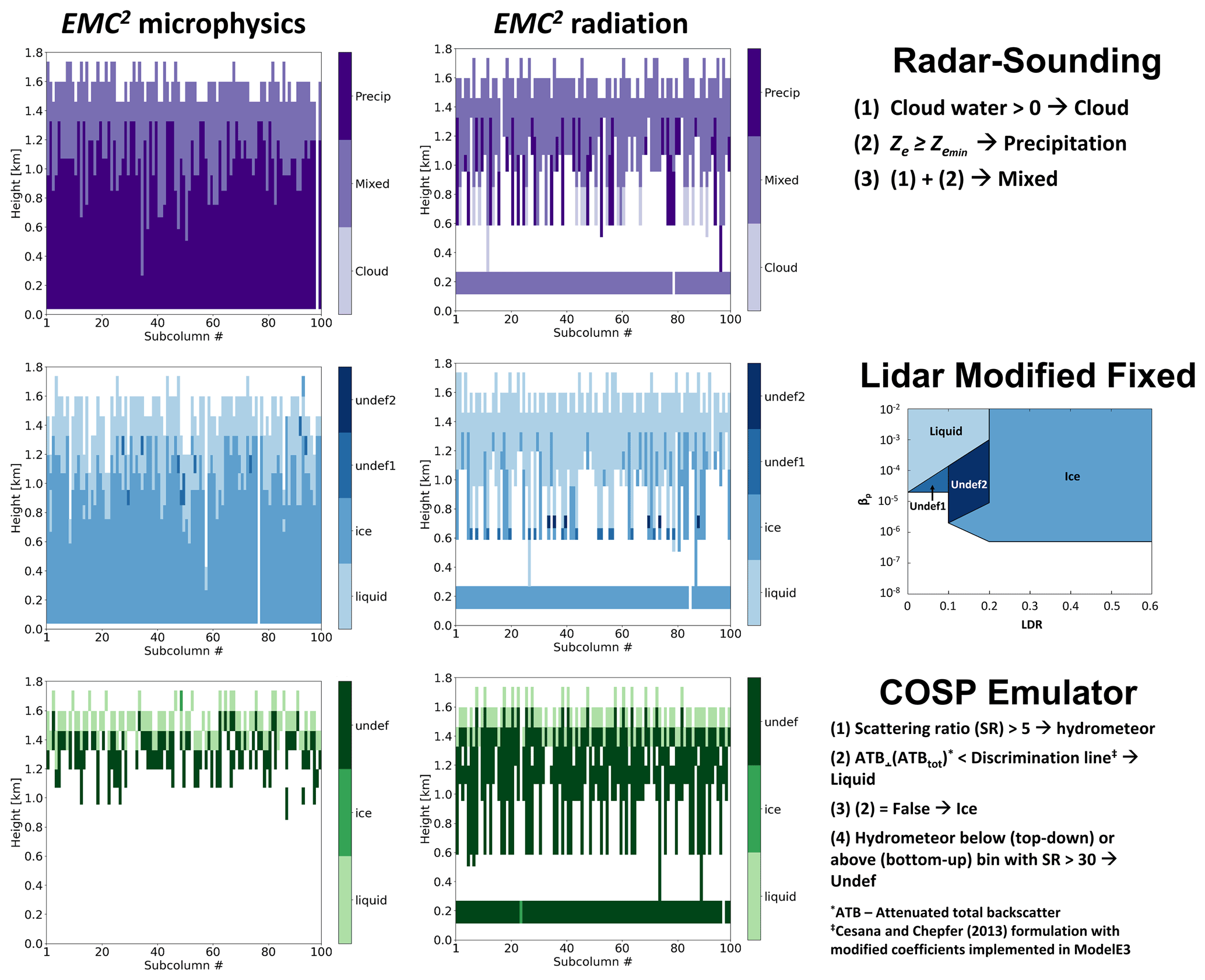
Figure 7Hydrometeor classification of ModelE3 configuration Tun3 SCM output for 05:00 UTC processed using EMC2's microphysics (left) and radiation (middle) approaches while considering signal attenuation and detectability: (from top to bottom) radar-sounding method, modified fixed lidar variable threshold method, and the COSP lidar simulator emulator (top-down view). (Right) Brief summary of each classification method.
Using each of the three classification methods, phase ratio statistics can be generated with EMC2 offering a method for analyzing the SCM simulation. Figure 8 portrays the temporal evolution of the SCM simulation from the view of the simulated instruments and classification methods using the microphysics or radiation approaches. When radar-sounding and fixed lidar threshold methods are applied while using the microphysics approach, the evolution of the simulated cloud appears self-consistent between the two methods and generally follows the prototypical appearance of nearly continuously precipitating liquid-bearing cloud layers with weakly varying cloud base height (e.g., de Boer et al., 2011; Fridlind and Ackerman, 2018; Silber et al., 2021a). Here, the radar-sounding skill is associated with the diminished cloud water fraction relative to the large fraction of the other hydrometeor classes (Fig. 3, right) and the method's ability to correctly detect cloud water layers. The capabilities of this method should nonetheless be considered carefully when directly compared with observations because realistic sounding profiles typically lack the fine temporal resolution emulated by EMC2 here, and while in situ observations can provide a robust characterization of liquid-bearing cloud layers, they can also produce sporadic false positive or negative cloud detections (e.g., Silber et al., 2020, Fig. S1; Vassel et al., 2019). In the case of the modified fixed lidar threshold method, the low-level phase ratio skill originates from the hydrometeor-bearing subcolumn bins being largely classified as “ice”. This classification decision is the result of the low and moderate-to-high LDR (e.g., Fig. 6) produced by the prevalence of ice hydrometeors relative to cloud water (Fig. 3, right) and the greater mass (and likely volume due to the spherical representation) of these hydrometeors relative to rain (Fig. 3, left).
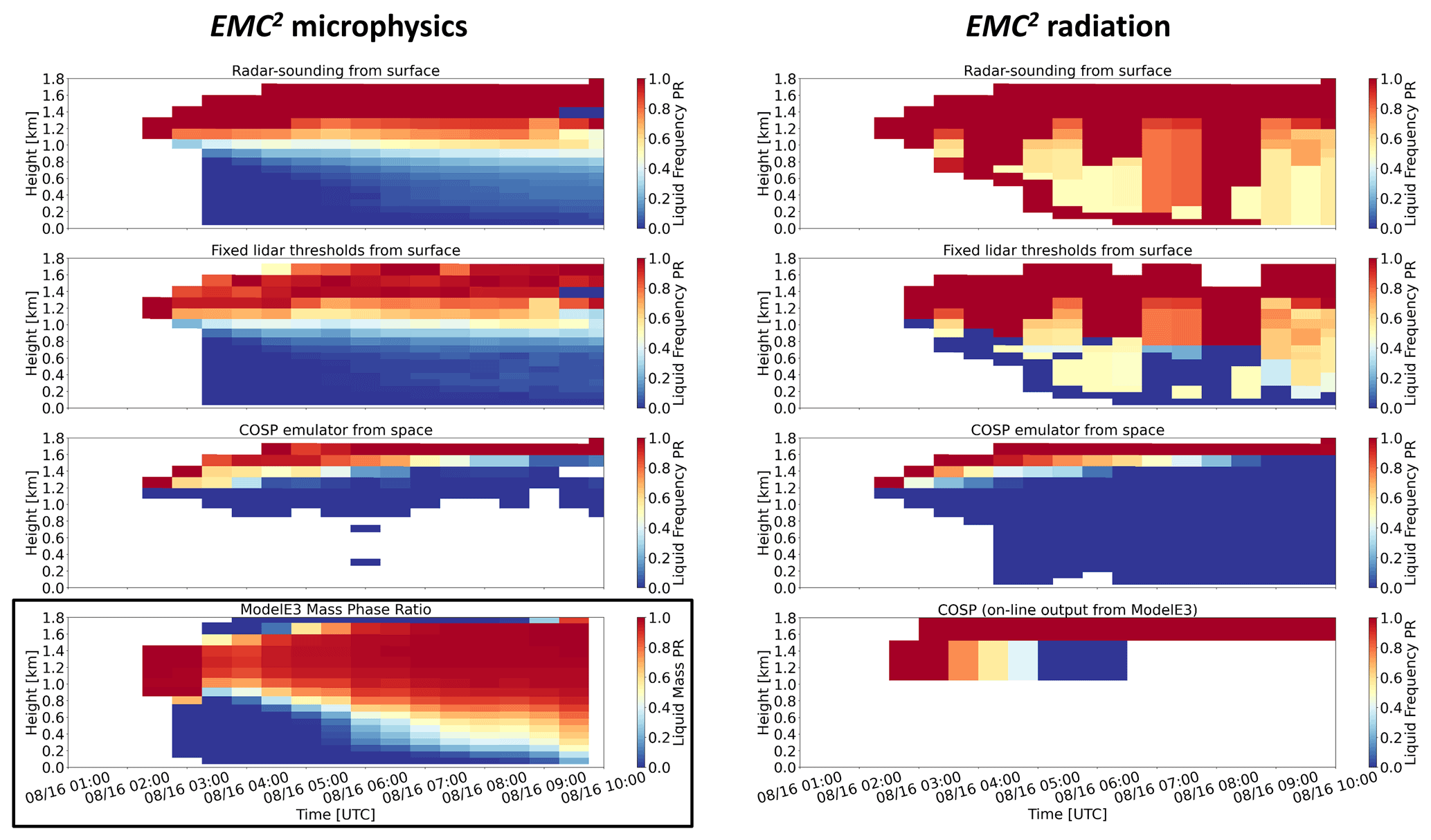
Figure 8Time–height curtain plots showing the liquid-bearing frequency phase ratio (calculated over all hydrometeor-bearing subcolumn bins) of ModelE3 configuration Tun3 SCM simulation using the microphysics (left) and radiation (right) approaches. The classification methods used to calculate the phase ratios are (from top to bottom) the radar-sounding method, the modified fixed lidar variable threshold method, the COSP lidar simulator emulator (top-down view), and the on-line COSP lidar simulator implemented in ModelE3, which is only processed using ModelE3's radiation approach. In this figure, the “mixed” class of the radar-sounding method is counted as liquid, while the “undefined” classes in the other two methods are treated as “non-liquid” even though in some cases they are more likely to be liquid-bearing (e.g., the “undefined1” class in the modified fixed lidar variable threshold method). The lower-left panel shows the mass phase ratio calculated using the ModelE3 output without EMC2 processing.
The COSP emulator using the microphysics approach with a top-down view is consistent with the example in Fig. 7, in which hydrometeor detection is limited by the optically thick and highly reflective cloud-top region, resembling observational retrievals (e.g., Cesana and Chepfer, 2013; Cesana et al., 2016).
Using the radiation approach, phase ratios more frequently show sharper transitions between the extreme values (all liquid or all non-liquid) stemming from the utilization of the generalized hydrometeor fraction. In the case of the radar-sounding method, for example, there is a distinct dominance of liquid-bearing bins, which only require any amount of cloud water to be classified as such. This dominance originates in the common occurrence of some cloud water mass mixing ratios in model grid cells throughout the SCM simulation (Fig. 3, left) combined with the implementation of the generalized hydrometeor fraction, which necessarily increases the overlap between cloud water and other hydrometeor classes. The limited number of model grid cells in which the subcolumn bins exhibit a more mixed behavior are the result of the randomized component of the subcolumn generator, which does not necessarily require overlap between cloud and precipitating hydrometeors (see Sect. 2.2). Based on these classification results, we suggest that the radar-sounding method could lead to hydrometeor classification favoring liquid-bearing classes when the radiation approach or similar model output with a generalized hydrometeor fraction is used.
The modified fixed lidar threshold method is relatively consistent with the microphysics approach (Fig. 8), even though some times (mainly around 06:00 and 10:00 UTC) are characterized by greater (smaller) relative liquid occurrence at lower (higher) model levels (phase ratio values closer to 0.5). These phase ratio differences relative to the microphysics approach are the result of the convolution of the generalized hydrometeor fraction and its deviation relative to the cloud water fraction (Fig. 3, right).
Using a top-down view, the COSP emulator agrees with both its application using the microphysics approach as well as the COSP output from the on-line simulator implemented in ModelE3, which utilizes the radiation approach (Fig. 8. Unlike the on-line simulator, the emulator detects some “undefined” hydrometeors at low levels (down to the surface), which can be explained by the lack of model interpolation onto a uniform vertical grid and/or small differences in the compiled simulator code related to signal attenuation (e.g., the accumulation of optical thickness).
We note that the treatment of the COSP emulator's “undefined” subcolumn bins as “ice” to produce phase ratio statistics leaves the impression that only ice hydrometeors exist below cloud top. However, a rather different impression of mostly liquid water dominance, though not as stark as in the radar-sounding method using the radiation approach, is perceived when the mass phase ratio calculated using the raw SCM output is examined (Fig. 8, lower left). Contrary to the COSP emulator, treating “undefined” bins as “ice” in the modified fixed lidar threshold method increases its apparent frequency phase ratio agreement with the mass phase ratio in multiple time–height bins. Phase classification depends on instrument measurement characteristics and limitations and hydrometeor properties such as their class, relative mixture with other hydrometeor classes, as well as their size distributions. Therefore, such an apparent agreement between different variables and phase occurrence metrics, as well as between the same variables and metrics based on different instruments and/or methodologies, should be taken with a grain of salt (cf. Cesana et al., 2021; see also Silber et al., 2021c).
Figure 8 demonstrates the sensitivity of phase ratio statistics to the classification method, the viewing direction of the examined instrument, and the method by which “liquid” and “non-liquid” or “ice” classes are being counted. It shows that the use of forward simulators alone is not a guarantee for an “apples-to-apples” comparison, which requires matching processing steps to ensure its robustness.
EMC2 provides an easy to use and flexible framework for the analysis of large-scale model output and its direct comparison with ground-based observations via the generation of subcolumns intended to explicitly represent a sub-grid scale variability, and the simulation of ground-based (and air- or space-borne) radars and lidars. EMC2's framework is already tailored to the MG2 two-moment microphysics while using single-particle scattering LUTs and has the proper infrastructure required for it to be customized to other similar schemes, as well as high-resolution model output. EMC2's option for using radiation scheme logic in the subcolumn generator and simulator enables direct comparison with other on-line active instrument simulators (e.g., the COSP lidar simulator) with a bottom-up or top-down view option that can bridge between different methodologies by evaluating differences between the outputs resulting from their implementation.
Because it is generally designed to emulate ground-based systems, EMC2 is suitable for the evaluation of column output extracted from global simulations against long-term ground-based datasets. The general adaptability of the software code to other climate models and instruments via the model and instrument Python classes renders EMC2 as a flexible framework to enable consistent and reproducible post-processing methods and evaluation across multiple models.
An AWARE case study was used to illustrate the application of EMC2 to LES and SCM simulations of a highly supercooled Antarctic cloud, including the utility of the program for hydrometeor classification using radar-sounding, lidar variable thresholds, and COSP emulator methods. The ModelE3 SCM using configuration Tun3 showed general agreement with the observations at the examined simulation time as well as with the baseline DHARMA LES used to develop this case study (see Silber et al., 2019a). The LES output can be processed with EMC2 after a few adaptations made only to an inherited Model class (see Sect. 2.1). Thus, although it was developed for large-scale models, EMC2 can also be used to compare cloud resolving or LES models with observations (as shown for DHARMA). EMC2 also allows the implementation of advanced scattering model calculations in the forward calculations via customized LUTs that could be matched to some scattering assumptions made by models, for example, the implementation of the MODIS C6 calculations in both ModelE3's radiation scheme and EMC2.
The AWARE case study presented here is suitable for simulation by any global model in SCM mode (see input file repository specified under code and data availability). Case study observations, as well as ModelE3 SCM and DHARMA LES inputs and outputs from EMC2 used to produce all examples above, are also provided for step-by-step illustration (see code and data availability). We plan that additional case study examples will similarly be provided to illustrate results under differing cloud regimes.
Planned future additions to EMC2 include an extension to ground-based scanning radars, a Mie scattering calculator, spectral broadening estimates for the radar simulator, and a multiple-scattering model for the lidar simulator, all of which will be configured for consistency with model physics and output fields. We invite the community to take advantage of the framework provided by EMC2 and to contribute to its further development and applications.
Table A1Acronyms and subscript abbreviations used in this article.
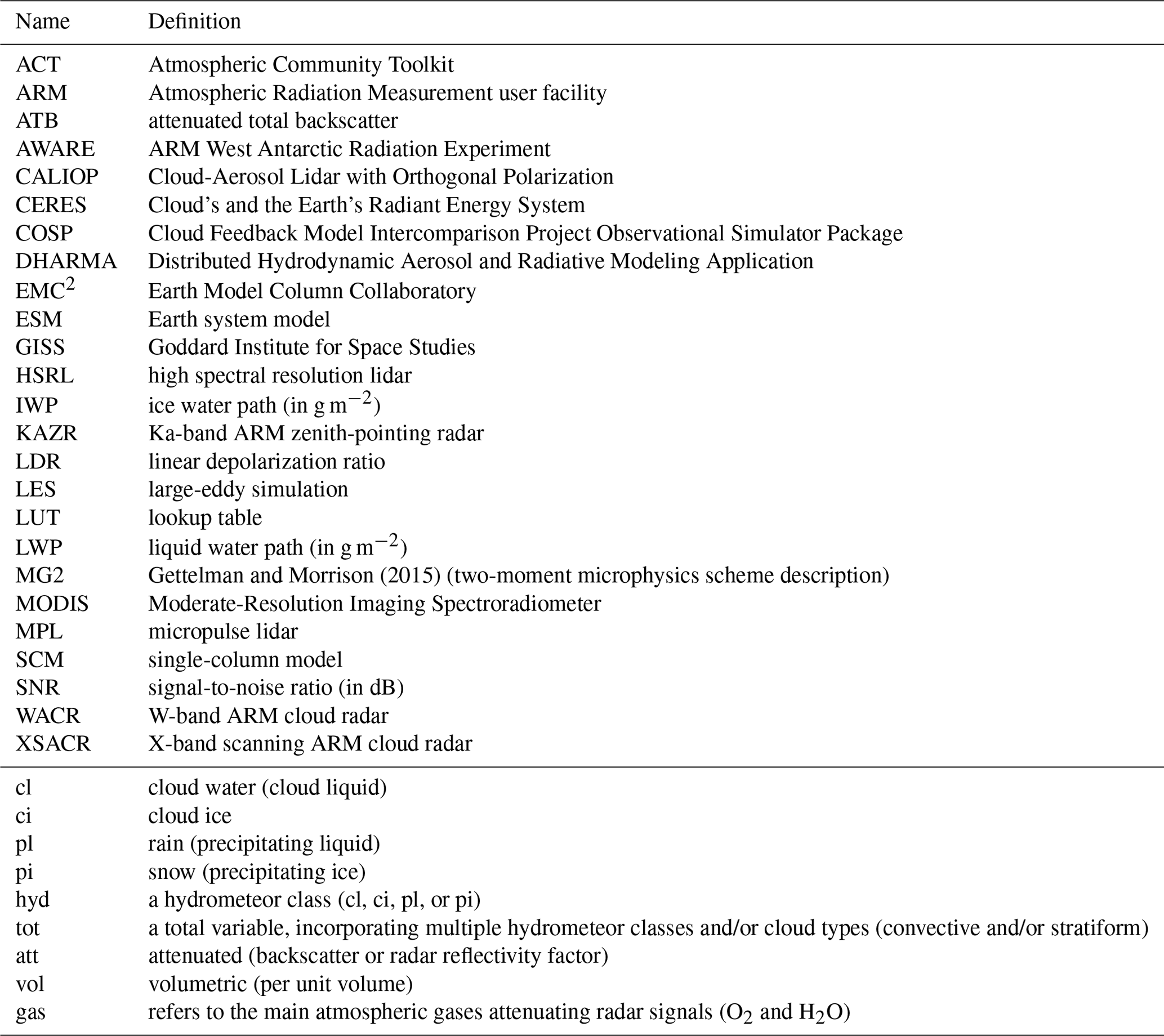
Table A2Symbols of variables and parameters used in this article and their units (unless explicitly stated otherwise in the text).
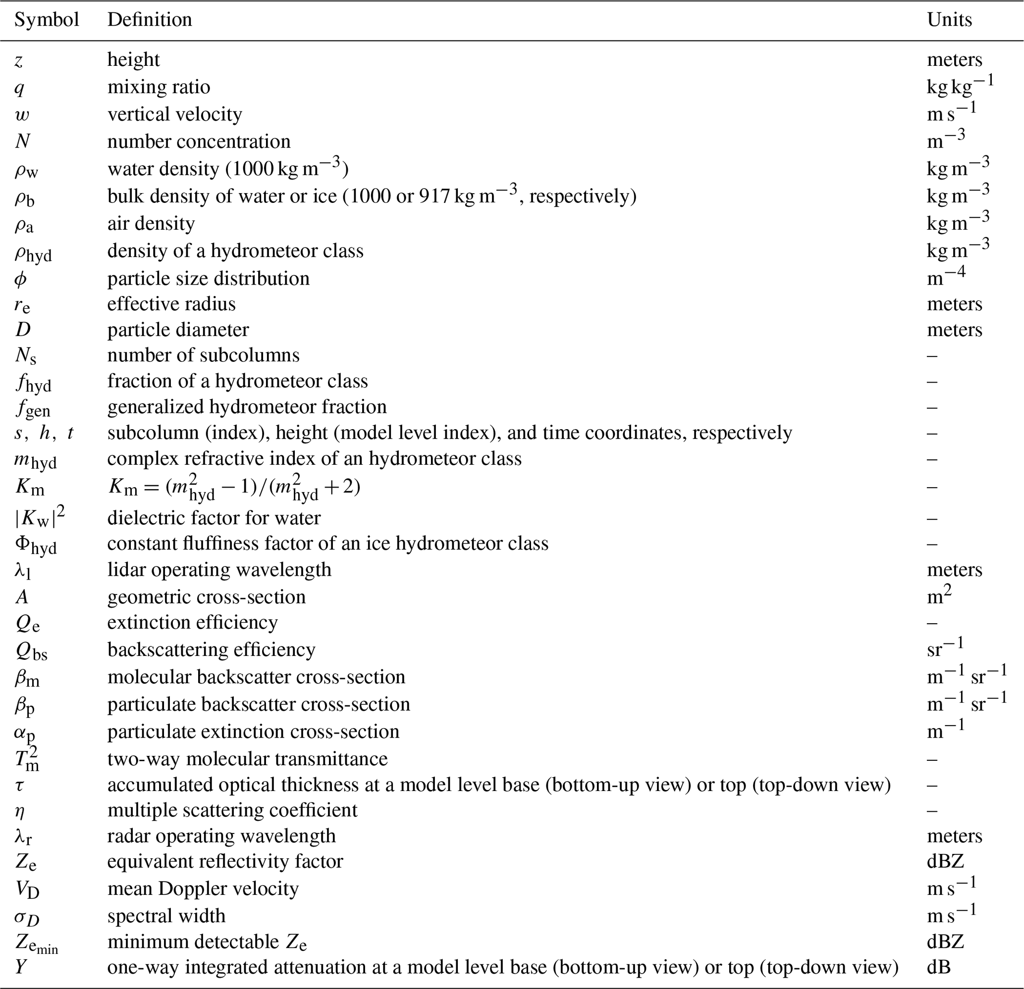

Figure B1Time series showing (a) liquid water path (LWP) and (b) ice water path (IWP) in each case study simulation using the DHARMA LES (baseline simulation in Silber et al., 2019a), and the four ModelE3 configurations (Tun1, Tun2, Tun3, and Phys). The Eulerian retrievals shown for 10:00 UTC (error bars denote uncertainty) correspond to the time at which the Lagrangian simulated domain approaches McMurdo Station (see Sect. 3.2). (c, d, e) Temperature, turbulent kinetic energy, and cloud water mixing ratio profiles at the end of the SCM and DHARMA LES simulations.
Figure B1 illustrates time series of liquid water path (LWP) and ice water path (IWP) from the ModelE3 SCM case study output using configurations Tun1, Tun2, Tun3, and Phys (see Sect. 3.3), as well as the temperature, turbulent kinetic energy (TKE), and cloud water mixing ratio profiles at the end of the simulation. Out of these four model configurations, only configurations Tun3 and Phys maintain substantial amounts of LWP in this highly supercooled cloud case study and agree with both the depicted DHARMA LES output and the observed LWP retrievals (see Silber et al., 2019a). Moreover, the SCM using each of these two configurations is able to develop a cloud-top inversion and TKE, both of which are driven by radiative cooling of cloud water, consistent with the DHARMA LES (see Fig. B1, bottom panels) and various polar cloud observations (e.g., Morrison et al., 2012; Silber et al., 2019a). All of ModelE3's configurations except for Tun1, which generates the largest amount of ice, are within the range of IWP estimated retrieval uncertainty. Out of those three model configurations, Tun3 is closest to the retrieved IWP and best matches the cloud formation and evolution in the LES. Because the supercooled cloud is developed faster in the SCM than in the LES model (see Fig. B1, top and middle), we choose to demonstrate EMC2 using the SCM output corresponding to 05:00 UTC. Figure B2 shows the mean lidar and radar variable profiles at that model time step from EMC2 for each of the four model configurations together with the time-averaged observed profiles. Using either the microphysics or radiation approach, configurations Tun3 and Phys best match the observations. Most of the radar and lidar variables calculated using these two configurations are largely consistent with each other, but overall, the Tun3 SCM output shows the best agreement with the mean observed profiles.
To summarize, two of ModelE3's final four configurations, that is, configurations Tun3 and Phys, show reasonable agreement with both the observed quantities as well as the LES output variables. Because configuration Tun3 performs slightly better, we focus on this model configuration for detailed comparison with LES and observations.
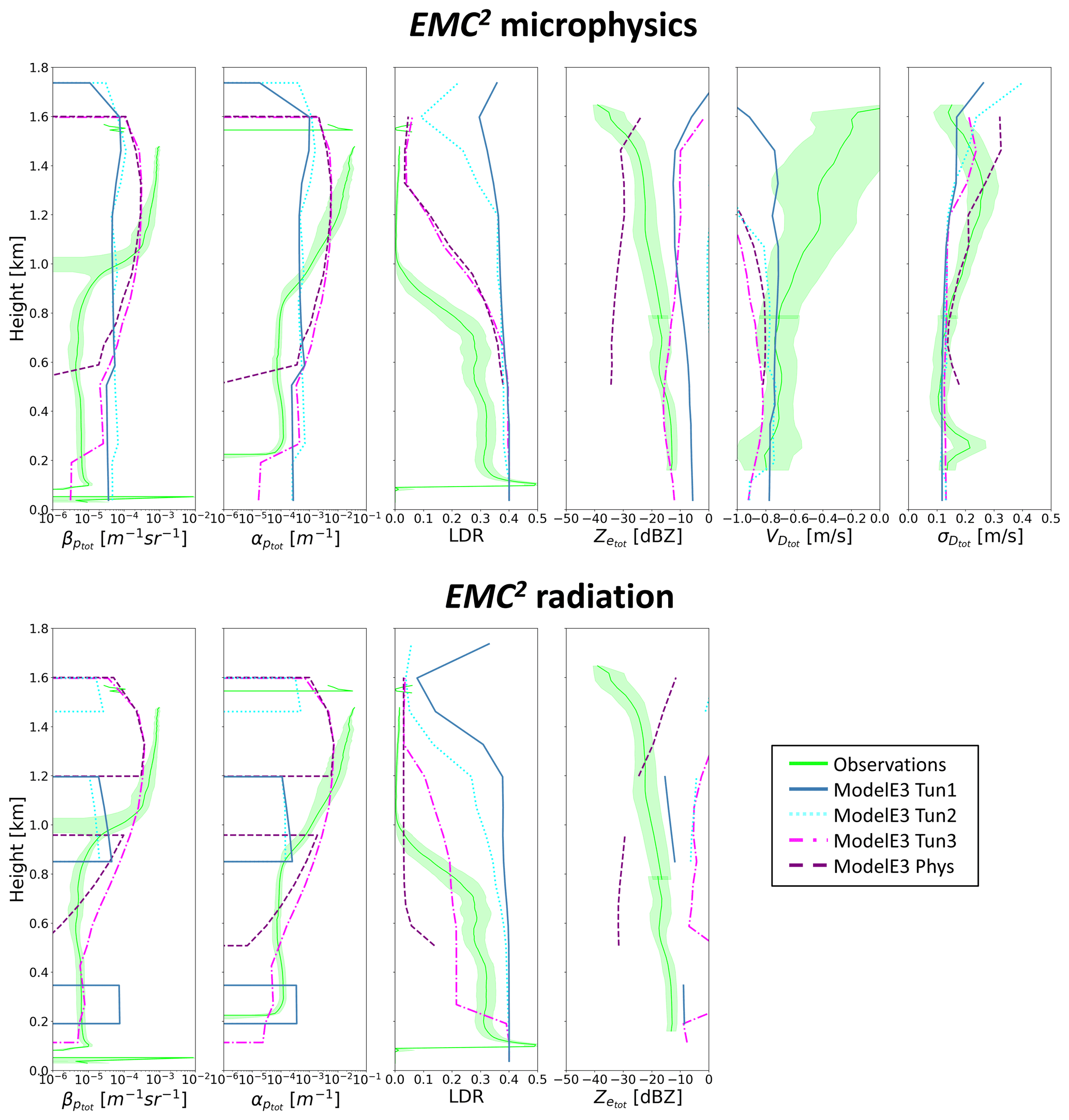
Figure B2Mean profiles of observed (time-averaged) and simulated (subcolumn-averaged) HSRL and KAZR variables calculated using EMC2 microphysics (top) and radiation (bottom) approaches using the four ModelE3 configurations (see legend), without applying a lidar and radar extinction or SNR masks, respectively.
The most recent EMC2 code (v. 1.2), which also supports the E3SM and CESM2 climate models as well as the Weather Research and Forecasting (WRF) model, is available on GitHub at https://github.com/columncolab/EMC2/ (last access: 1 December 2021). The EMC2 Version 1.1 code described and used in this study, together with KAZR and HSRL measurements, EMC2-processed ModelE3 and DHARMA LES model output data files, and a Jupyter Notebook demonstrating the reproduction of the plots in this article using EMC2, is available at Zenodo (https://doi.org/10.5281/zenodo.5115252; Silber et al., 2021b). The SCM initialization files (sounding + forcing) required to run the case study simulation are available at the Mendeley Data repository under https://doi.org/10.17632/gz4gdn3jvz.1 (Silber, 2021).
IS and AMF conceptualized the simulator and subcolumn generator with essential support from ASA. RCJ and SC conceptualized the open-source Python framework. IS and RCJ developed the EMC2 code. ASA contributed to structuring general climate model logic and ModelE3's logic specifics. JV supported the consistency and conceptual implementation of the instrument logic. JD provided the Yang et al. (2013) and Ding et al. (2017) single-particle scattering LUTs and added essential information required to reproduce and maintain the MODIS C6 consistency. IS prepared the manuscript with contributions from RCJ. All authors reviewed and edited the manuscript.
The contact author has declared that neither they nor their co-authors have any competing interests.
Publisher's note: Copernicus Publications remains neutral with regard to jurisdictional claims in published maps and institutional affiliations.
We thank Gregory Elsasser, Bastiaan van Diedenhoven, Maxwell Kelley, and Ed Eloranta for helpful discussions. Israel Silber is supported by DOE grants DE-SC0018046 and DE-SC0021004. Scott Collis and Robert C. Jackson were supported by the U.S. Department of Energy (DOE) Atmospheric System Research (ASR), Office of Science, Office of Biological and Environmental Research (BER) program, under contract DE-AC02-06CH11357 awarded to Argonne National Laboratory. Ann M. Fridlind and Andrew S. Ackerman were supported by the NASA Modeling Analysis and Prediction Program. Resources supporting this work were provided by the NASA Center for Climate Simulation (NCCS) at Goddard Space Flight Center.
This research has been supported by the U.S. Department of Energy (grant nos. DE-SC0018046, DE-SC0021004, and DE-AC02-06CH11357).
This paper was edited by Paul Ullrich and reviewed by Roger Marchand and one anonymous referee.
Amante, C.: ETOPO1 1 arc-minute global relief model: procedures, data sources and analysis, NOAA Technical Memorandum NESDIS NGDC-24, National Geophysical Data Center [data set], NOAA, Tech. rep., https://doi.org/10.7289/V5C8276M, 2009. a
Bodas-Salcedo, A., Webb, M. J., Brooks, M. E., Ringer, M. A., Williams, K. D., Milton, S. F., and Wilson, D. R.: Evaluating cloud systems in the Met Office global forecast model using simulated CloudSat radar reflectivities, J. Geophys. Res.-Atmos., 92, 1023–1043, https://doi.org/10.1029/2007JD009620, 2008. a
Bodas-Salcedo, A., Webb, M. J., Bony, S., Chepfer, H., Dufresne, J.-L., Klein, S. A., Zhang, Y., Marchand, R., Haynes, J. M., Pincus, R., and John, V. O.: COSP: Satellite simulation software for model assessment, B. Am. Meteorol. Soc., 92, 1023–1043, https://doi.org/10.1175/2011BAMS2856.1, 2011. a, b
Bodas-Salcedo, A., Williams, K. D., Ringer, M. A., Beau, I., Cole, J. N. S., Dufresne, J.-L., Koshiro, T., Stevens, B., Wang, Z., and Yokohata, T.: Origins of the Solar Radiation Biases over the Southern Ocean in CFMIP2 Models, J. Climate, 27, 41–56, https://doi.org/10.1175/JCLI-D-13-00169.1, 2014. a
Bohren, C. F. and Battan, L. J.: Radar Backscattering by Inhomogeneous Precipitation Particles, J. Atmos. Sci., 37, 1821–1827, https://doi.org/10.1175/1520-0469(1980)037<1821:RBBIPP>2.0.CO;2, 1980. a
Bohren, C. F. and Huffman, D. R.: Absorption and Scattering of Light by Small Particles, John Wiley & Sons, Ltd, Weinheim, Germany, https://doi.org/10.1002/9783527618156, 1983. a
Burns, D., Kollias, P., Tatarevic, A., Battaglia, A., and Tanelli, S.: The performance of the EarthCARE Cloud Profiling Radar in marine stratiform clouds, J. Geophys. Res.-Atmos., 121, 14525–14537, https://doi.org/10.1002/2016JD025090, 2016. a, b
Campbell, J. R., Hlavka, D. L., Welton, E. J., Flynn, C. J., Turner, D. D., Spinhirne, J. D., Scott, V. S., and Hwang, I. H.: Full-Time, Eye-Safe Cloud and Aerosol Lidar Observation at Atmospheric Radiation Measurement Program Sites: Instruments and Data Processing, J. Atmos. Ocean. Tech., 19, 431–442, https://doi.org/10.1175/1520-0426(2002)019<0431:FTESCA>2.0.CO2, 2002. a
Cesana, G. and Chepfer, H.: Evaluation of the cloud thermodynamic phase in a climate model using CALIPSO-GOCCP, J. Geophys. Res.-Atmos., 118, 7922–7937, https://doi.org/10.1002/jgrd.50376, 2013. a, b
Cesana, G. and Waliser, D. E.: Characterizing and understanding systematic biases in the vertical structure of clouds in CMIP5/CFMIP2 models, Geophys. Res. Lett., 43, 10538–10546, https://doi.org/10.1002/2016GL070515, 2016. a
Cesana, G., Kay, J. E., Chepfer, H., English, J. M., and de Boer, G.: Ubiquitous low-level liquid-containing Arctic clouds: New observations and climate model constraints from CALIPSO-GOCCP, Geophys. Res. Lett., 39, L20804, https://doi.org/10.1029/2012GL053385, 2012. a
Cesana, G., Chepfer, H., Winker, D., Getzewich, B., Cai, X., Jourdan, O., Mioche, G., Okamoto, H., Hagihara, Y., Noel, V., and Reverdy, M.: Using in situ airborne measurements to evaluate three cloud phase products derived from CALIPSO, J. Geophys. Res.-Atmos., 121, 5788–5808, https://doi.org/10.1002/2015JD024334, 2016. a
Cesana, G., Del Genio, A. D., Ackerman, A. S., Kelley, M., Elsaesser, G., Fridlind, A. M., Cheng, Y., and Yao, M.-S.: Evaluating models' response of tropical low clouds to SST forcings using CALIPSO observations, Atmos. Chem. Phys., 19, 2813–2832, https://doi.org/10.5194/acp-19-2813-2019, 2019. a, b, c
Cesana, G. V., Ackerman, A. S., Fridlind, A. M., Silber, I., and Kelley, M.: Snow Reconciles Observed and Simulated Phase Partitioning and Increases Cloud Feedback, Geophys. Res. Lett., 48, e2021GL094876, https://doi.org/10.1029/2021GL094876, 2021. a
Chen, Y.-S., Verlinde, J., Clothiaux, E. E., Ackerman, A. S., Fridlind, A. M., Chamecki, M., Kollias, P., Kirkpatrick, M. P., Chen, B.-C., Yu, G., and Avramov, A.: On the forward modeling of radar Doppler spectrum width from LES: Implications for model evaluation, J. Geophys. Res.-Atmos., 123, 7444–7461, https://doi.org/10.1029/2017JD028104, 2018. a
Chepfer, H., Bony, S., Winker, D., Chiriaco, M., Dufresne, J.-L., and Sèze, G.: Use of CALIPSO lidar observations to evaluate the cloudiness simulated by a climate model, Geophys. Res. Lett., 35, L15704, https://doi.org/10.1029/2008GL034207, 2008. a
Danabasoglu, G., Lamarque, J.-F., Bacmeister, J., Bailey, D. A., DuVivier, A. K., Edwards, J., Emmons, L. K., Fasullo, J., Garcia, R., Gettelman, A., Hannay, C., Holland, M. M., Large, W. G., Lauritzen, P. H., Lawrence, D. M., Lenaerts, J. T. M., Lindsay, K., Lipscomb, W. H., Mills, M. J., Neale, R., Oleson, K. W., Otto-Bliesner, B., Phillips, A. S., Sacks, W., Tilmes, S., van Kampenhout, L., Vertenstein, M., Bertini, A., Dennis, J., Deser, C., Fischer, C., Fox-Kemper, B., Kay, J. E., Kinnison, D., Kushner, P. J., Larson, V. E., Long, M. C., Mickelson, S., Moore, J. K., Nienhouse, E., Polvani, L., Rasch, P. J., and Strand, W. G.: The Community Earth System Model Version 2 (CESM2), J. Adv. Model. Earth Sy., 12, e2019MS001916, https://doi.org/10.1029/2019MS001916, 2020. a
de Boer, G., Morrison, H., Shupe, M. D., and Hildner, R.: Evidence of liquid dependent ice nucleation in high-latitude stratiform clouds from surface remote sensors, Geophys. Res. Lett., 38, L01803, https://doi.org/10.1029/2010GL046016, 2011. a
Derr, V. E., Abshire, N. L., Cupp, R. E., and McNice, G. T.: Depolarization of Lidar Returns from Virga and Source Cloud, J. Appl. Meteorol. Clim., 15, 1200–1203, https://doi.org/10.1175/1520-0450(1976)015<1200:DOLRFV>2.0.CO;2, 1976. a, b
Ding, J., Bi, L., Yang, P., Kattawar, G. W., Weng, F., Liu, Q., and Greenwald, T.: Single-scattering properties of ice particles in the microwave regime: Temperature effect on the ice refractive index with implications in remote sensing, J. Quant. Spectrosc. Ra., 190, 26–37, https://doi.org/10.1016/j.jqsrt.2016.11.026, 2017. a, b
Doviak, R. J. and Zrnić, D. S.: Doppler Radar and Weather Observations, 2nd Edn. Academic Press, San Diego, https://doi.org/10.1016/C2009-0-22358-0, 1993. a
Eloranta, E. W.: Practical model for the calculation of multiply scattered lidar returns, Appl. Optics, 37, 2464–2472, https://doi.org/10.1364/AO.37.002464, 1998. a
Eloranta, E. W.: High spectral resolution lidar, in: Lidar: Range-Resolved Optical Remote Sensing of the Atmosphere, Springer New York, New York, NY, 143–163, 2005. a
Elsaesser, G. S., Genio, A. D. D., Jiang, J. H., and van Lier-Walqui, M.: An Improved Convective Ice Parameterization for the NASA GISS Global Climate Model and Impacts on Cloud Ice Simulation, J. Climate, 30, 317–336, https://doi.org/10.1175/JCLI-D-16-0346.1, 2017. a
Falconi, M. T., von Lerber, A., Ori, D., Marzano, F. S., and Moisseev, D.: Snowfall retrieval at X, Ka and W bands: consistency of backscattering and microphysical properties using BAECC ground-based measurements, Atmos. Meas. Tech., 11, 3059–3079, https://doi.org/10.5194/amt-11-3059-2018, 2018. a, b
Fan, J., Ghan, S., Ovchinnikov, M., Liu, X., Rasch, P. J., and Korolev, A.: Representation of Arctic mixed-phase clouds and the Wegener-Bergeron-Findeisen process in climate models: Perspectives from a cloud-resolving study, J. Geophys. Res.-Atmos., 116, D00T07, https://doi.org/10.1029/2010JD015375, 2011. a
Flynn, C. J., Mendozaa, A., Zhengb, Y., and Mathurb, S.: Novel polarization-sensitive micropulse lidar measurement technique, Opt. Express, 15, 2785–2790, https://doi.org/10.1364/OE.15.002785, 2007. a
Fridlind, A. M. and Ackerman, A. S.: Simulations of Arctic Mixed-Phase Boundary Layer Clouds: Advances in Understanding and Outstanding Questions, chap. 7, in: Mixed-Phase Clouds, edited by: Andronache, C., Elsevier, 153–183, https://doi.org/10.1016/B978-0-12-810549-8.00007-6, 2018. a
Gettelman, A. and Morrison, H.: Advanced Two-Moment Bulk Microphysics for Global Models, Part I: Off-Line Tests and Comparison with Other Schemes, J. Climate, 28, 1268–1287, https://doi.org/10.1175/JCLI-D-14-00102.1, 2015. a, b, c
Golaz, J.-C., Caldwell, P. M., Van Roekel, L. P., Petersen, M. R., Tang, Q., Wolfe, J. D., Abeshu, G., Anantharaj, V., Asay-Davis, X. S., Bader, D. C., Baldwin, S. A., Bisht, G., Bogenschutz, P. A., Branstetter, M., Brunke, M. A., Brus, S. R., Burrows, S. M., Cameron-Smith, P. J., Donahue, A. S., Deakin, M., Easter, R. C., Evans, K. J., Feng, Y., Flanner, M., Foucar, J. G., Fyke, J. G., Griffin, B. M., Hannay, C., Harrop, B. E., Hoffman, M. J., Hunke, E. C., Jacob, R. L., Jacobsen, D. W., Jeffery, N., Jones, P. W., Keen, N. D., Klein, S. A., Larson, V. E., Leung, L. R., Li, H.-Y., Lin, W., Lipscomb, W. H., Ma, P.-L., Mahajan, S., Maltrud, M. E., Mametjanov, A., McClean, J. L., McCoy, R. B., Neale, R. B., Price, S. F., Qian, Y., Rasch, P. J., Reeves Eyre, J. E. J., Riley, W. J., Ringler, T. D., Roberts, A. F., Roesler, E. L., Salinger, A. G., Shaheen, Z., Shi, X., Singh, B., Tang, J., Taylor, M. A., Thornton, P. E., Turner, A. K., Veneziani, M., Wan, H., Wang, H., Wang, S., Williams, D. N., Wolfram, P. J., Worley, P. H., Xie, S., Yang, Y., Yoon, J.-H., Zelinka, M. D., Zender, C. S., Zeng, X., Zhang, C., Zhang, K., Zhang, Y., Zheng, X., Zhou, T., and Zhu, Q.: The DOE E3SM Coupled Model Version 1: Overview and Evaluation at Standard Resolution, J. Adv. Model. Earth Sy., 11, 2089–2129, https://doi.org/10.1029/2018MS001603, 2019. a
Hansen, J. E.: Multiple Scattering of Polarized Light in Planetary Atmospheres Part II. Sunlight Reflected by Terrestrial Water Clouds, J. Atmos. Sci., 28, 1400–1426, https://doi.org/10.1175/1520-0469(1971)028<1400:MSOPLI>2.0.CO;2, 1971. a
Heiblum, R. H., Altaratz, O., Koren, I., Feingold, G., Kostinski, A. B., Khain, A. P., Ovchinnikov, M., Fredj, E., Dagan, G., Pinto, L., Yaish, R., and Chen, Q.: Characterization of cumulus cloud fields using trajectories in the center of gravity versus water mass phase space: 2. Aerosol effects on warm convective clouds, J. Geophys. Res.-Atmos., 121, 6356–6373, https://doi.org/10.1002/2015JD024193, 2016. a
Hersbach, H., Bell, B., Berrisford, P., Hirahara, S., Horányi, A., Muñoz-Sabater, J., Nicolas, J., Peubey, C., Radu, R., Schepers, D., Simmons, A., Soci, C., Abdalla, S., Abellan, X., Balsamo, G., Bechtold, P., Biavati, G., Bidlot, J., Bonavita, M., De Chiara, G., Dahlgren, P., Dee, D., Diamantakis, M., Dragani, R., Flemming, J., Forbes, R., Fuentes, M., Geer, A., Haimberger, L., Healy, S., Hogan, R. J., Hólm, E., Janisková, M., Keeley, S., Laloyaux, P., Lopez, P., Lupu, C., Radnoti, G., de Rosnay, P., Rozum, I., Vamborg, F., Villaume, S., and Thépaut, J.-N.: The ERA5 global reanalysis, Q. J. Roy. Meteor. Soc., 146, 1999–2049, https://doi.org/10.1002/qj.3803, 2020. a
Hillman, B. R., Marchand, R. T., and Ackerman, T. P.: Sensitivities of Simulated Satellite Views of Clouds to Subgrid-Scale Overlap and Condensate Heterogeneity, J. Geophys. Res.-Atmos., 123, 7506–7529, https://doi.org/10.1029/2017JD027680, 2018. a, b
Holz, R. E., Platnick, S., Meyer, K., Vaughan, M., Heidinger, A., Yang, P., Wind, G., Dutcher, S., Ackerman, S., Amarasinghe, N., Nagle, F., and Wang, C.: Resolving ice cloud optical thickness biases between CALIOP and MODIS using infrared retrievals, Atmos. Chem. Phys., 16, 5075–5090, https://doi.org/10.5194/acp-16-5075-2016, 2016. a
Hoyer, S. and Hamman, J.: xarray: N-D labeled arrays and datasets in Python, J. Open Res. Softw., 5, p. 10, https://doi.org/10.5334/jors.148, 2017. a
Khairoutdinov, M. and Kogan, Y.: A New Cloud Physics Parameterization in a Large-Eddy Simulation Model of Marine Stratocumulus, Mon. Weather Rev., 128, 229–243, https://doi.org/10.1175/1520-0493(2000)128<0229:ANCPPI>2.0.CO;2, 2000. a
Klein, S. A. and Jakob, C.: Validation and Sensitivities of Frontal Clouds Simulated by the ECMWF Model, Mon. Weather Rev., 127, 2514–2531, https://doi.org/10.1175/1520-0493(1999)127<2514:VASOFC>2.0.CO;2, 1999. a
Klein, S. A., Zhang, Y., Zelinka, M. D., Pincus, R., Boyle, J., and Gleckler, P. J.: Are climate model simulations of clouds improving? An evaluation using the ISCCP simulator, J. Geophys. Res.-Atmos., 118, 1329–1342, https://doi.org/10.1002/jgrd.50141, 2013. a, b
Kuma, P., McDonald, A. J., Morgenstern, O., Querel, R., Silber, I., and Flynn, C. J.: Ground-based lidar processing and simulator framework for comparing models and observations (ALCF 1.0), Geosci. Model Dev., 14, 43–72, https://doi.org/10.5194/gmd-14-43-2021, 2021. a
Lamer, K.: Relative Occurrence of Liquid, Ice and Mixed-phase Conditions Within Cloud and Precipitation Regimes: Long Term Ground-based Observations for GCM Model Evaluation, available at: https://etda.libraries.psu.edu/catalog/16162kxl5431 (last access: 1 December 2021), 2019. a, b
Lin, J.-L., Qian, T., and Shinoda, T.: Stratocumulus Clouds in Southeastern Pacific Simulated by Eight CMIP5–CFMIP Global Climate Models, J. Climate, 27, 3000–3022, https://doi.org/10.1175/JCLI-D-13-00376.1, 2014. a
Lin, L., Gettelman, A., Xu, Y., Wu, C., Wang, Z., Rosenbloom, N., Bates, S. C., and Dong, W.: CAM6 simulation of mean and extreme precipitation over Asia: sensitivity to upgraded physical parameterizations and higher horizontal resolution, Geosci. Model Dev., 12, 3773–3793, https://doi.org/10.5194/gmd-12-3773-2019, 2019. a, b
Lubin, D., Zhang, D., Silber, I., Scott, R. C., Kalogeras, P., Battaglia, A., Bromwich, D. H., Cadeddu, M., Eloranta, E., Fridlind, A., Frossard, A., Hines, K. M., Kneifel, S., Leaitch, W. R., Lin, W., Nicolas, J., Powers, H., Quinn, P. K., Rowe, P., Russell, L. M., Sharma, S., Verlinde, J., and Vogelmann, A. M.: AWARE: The Atmospheric Radiation Measurement (ARM) West Antarctic Radiation Experiment, B. Am. Meteorol. Soc., 101, E1069–E1091, https://doi.org/10.1175/BAMS-D-18-0278.1, 2020. a
Mätzler, C. (Ed.): Thermal Microwave Radiation: Applications for Remote Sensing, Electromagnetic Waves, Institution of Engineering and Technology, available at: https://digital-library.theiet.org/content/books/ew/pbew052e (last access: 1 December 2021), 2006. a
Mech, M., Maahn, M., Kneifel, S., Ori, D., Orlandi, E., Kollias, P., Schemann, V., and Crewell, S.: PAMTRA 1.0: the Passive and Active Microwave radiative TRAnsfer tool for simulating radiometer and radar measurements of the cloudy atmosphere, Geosci. Model Dev., 13, 4229–4251, https://doi.org/10.5194/gmd-13-4229-2020, 2020. a
Morris, V. R.: Ceilometer Instrument Handbook, DOE/SC-ARM-TR-020, DOE Office of Science, Office of Biological and Environmental Research, https://doi.org/10.2172/1036530, 2016. a
Morrison, H. and Gettelman, A.: A New Two-Moment Bulk Stratiform Cloud Microphysics Scheme in the Community Atmosphere Model, Version 3 (CAM3). Part I: Description and Numerical Tests, J. Climate, 21, 3642–3659, https://doi.org/10.1175/2008JCLI2105.1, 2008. a, b, c, d
Morrison, H., Thompson, G., and Tatarskii, V.: Impact of Cloud Microphysics on the Development of Trailing Stratiform Precipitation in a Simulated Squall Line: Comparison of One- and Two-Moment Schemes, Mon. Weather Rev., 137, 991–1007, https://doi.org/10.1175/2008MWR2556.1, 2009. a
Morrison, H., de Boer, G., Feingold, G., Harrington, J., Shupe, M. D., and Sulia, K.: Resilience of persistent Arctic mixed-phase clouds, Nat. Geosci., 5, 11–17, https://doi.org/10.1038/ngeo1332, 2012. a
Myers, T. A., Scott, R. C., Zelinka, M. D., Klein, S. A., Norris, J. R., and Caldwell, P. M.: Observational constraints on low cloud feedback reduce uncertainty of climate sensitivity, Nat. Clim. Change, 11, 501–507, https://doi.org/10.1038/s41558-021-01039-0, 2021. a
Newsom, R. K.: Raman Lidar (RL) Handbook, DOE/SC-ARM-TR-038, DOE Office of Science, Office of Biological and Environmental Research, United States, https://doi.org/10.2172/1020561, 2009. a
Noel, V., Roy, G., Bissonnette, L., Chepfer, H., and Flamant, P.: Analysis of lidar measurements of ice clouds at multiple incidence angles, Geophys. Res. Lett., 29, 52-1–52-4, https://doi.org/10.1029/2002GL014828, 2002. a
Nott, G. J. and Duck, T. J.: Lidar studies of the polar troposphere, Meteorol. Appl., 18, 383–405, https://doi.org/10.1002/met.289, 2011. a
Oue, M., Tatarevic, A., Kollias, P., Wang, D., Yu, K., and Vogelmann, A. M.: The Cloud-resolving model Radar SIMulator (CR-SIM) Version 3.3: description and applications of a virtual observatory, Geosci. Model Dev., 13, 1975–1998, https://doi.org/10.5194/gmd-13-1975-2020, 2020. a
Penndorf, R.: Tables of the Refractive Index for Standard Air and the Rayleigh Scattering Coefficient for the Spectral Region between 0.2 and 20.0 µ and Their Application to Atmospheric Optics, J. Opt. Soc. Am., 47, 176–182, https://doi.org/10.1364/JOSA.47.000176, 1957. a
Platnick, S., King, M. D., Ackerman, S. A., Menzel, W. P., Baum, B. A., Riedi, J. C., and Frey, R. A.: The MODIS cloud products: algorithms and examples from Terra, IEEE T. Geosci. Remote, 41, 459–473, https://doi.org/10.1109/TGRS.2002.808301, 2003. a
Platnick, S., Meyer, K. G., King, M. D., Wind, G., Amarasinghe, N., Marchant, B., Arnold, G. T., Zhang, Z., Hubanks, P. A., Holz, R. E., Yang, P., Ridgway, W. L., and Riedi, J.: The MODIS Cloud Optical and Microphysical Products: Collection 6 Updates and Examples From Terra and Aqua, IEEE T. Geosci. Remote, 55, 502–525, https://doi.org/10.1109/TGRS.2016.2610522, 2017. a
Razenkov, I. I. and Eloranta, E. W.: High spectral resolution lidar at the university of wisconsin-madison, EPJ Web Conf., 176, 01024, https://doi.org/10.1051/epjconf/201817601024, 2018. a
Rowe, P. M., Fergoda, M., and Neshyba, S.: Temperature-Dependent Optical Properties of Liquid Water From 240 to 298 K, J. Geophys. Res.-Atmos., 125, e2020JD032624, https://doi.org/10.1029/2020JD032624,2020. a
Rémillard, J. and Tselioudis, G.: Cloud Regime Variability over the Azores and Its Application to Climate Model Evaluation, J. Climate, 28, 9707–9720, https://doi.org/10.1175/JCLI-D-15-0066.1, 2015. a
Sassen, K.: Polarization in lidar: a review, in: Polarization Science and Remote Sensing, edited by: Shaw, J. A. and Tyo, J. S., International Society for Optics and Photonics, SPIE, 5158, 151–160, https://doi.org/10.1117/12.507006, 2003. a
Segelstein, D. J.: The complex refractive index of water, PhD thesis, University of Missouri–Kansas City, http://hdl.handle.net/10355/11599 (last access: 1 December 2021), 1981. a, b
Seifert, A. and Beheng, K. D.: A double-moment parameterization for simulating autoconversion, accretion and selfcollection, Atmos. Res., 59–60, 265–281, https://doi.org/10.1016/S0169-8095(01)00126-0, 2001. a
Shupe, M. D.: A ground-based multisensor cloud phase classifier, Geophys. Res. Lett., 34, L22809, https://doi.org/10.1029/2007GL031008, 2007. a
Silber, I.: AWARE Highly Supercooled Cloud Case Study Model Initialization Files for SCMs, Mendeley Data V1 [data set], https://doi.org/10.17632/gz4gdn3jvz.1, 2021. a, b
Silber, I., Verlinde, J., Eloranta, E. W., and Cadeddu, M.: Antarctic cloud macrophysical, thermodynamic phase, and atmospheric inversion coupling properties at McMurdo Station, Part I: Principal data processing and climatology, J. Geophys. Res.-Atmos., 123, 6099–6121, https://doi.org/10.1029/2018JD028279, 2018a. a, b
Silber, I., Verlinde, J., Eloranta, E. W., Flynn, C. J., and Flynn, D. M.: Polar Liquid Cloud Base Detection Algorithms for High Spectral Resolution or Micropulse Lidar Data, J. Geophys. Res.-Atmos., 123, 4310–4322, https://doi.org/10.1029/2017JD027840, 2018b. a, b
Silber, I., Fridlind, A. M., Verlinde, J., Ackerman, A. S., Chen, Y.-S., Bromwich, D. H., Wang, S.-H., Cadeddu, M., and Eloranta, E. W.: Persistent Supercooled Drizzle at Temperatures Below −25 ∘C Observed at McMurdo Station, Antarctica, J. Geophys. Res.-Atmos., 124, 10878–10895, https://doi.org/10.1029/2019JD030882, 2019a. a, b, c, d, e, f, g, h, i, j, k, l, m, n, o, p, q, r, s
Silber, I., Verlinde, J., Wang, S.-H., Bromwich, D. H., Fridlind, A. M., Cadeddu, M., Eloranta, E. W., and Flynn, C. J.: Cloud Influence on ERA5 and AMPS Surface Downwelling Longwave Radiation Biases in West Antarctica, J. Climate, 32, 7935–7949, https://doi.org/10.1175/JCLI-D-19-0149.1, 2019b. a
Silber, I., Fridlind, A. M., Verlinde, J., Russell, L. M., and Ackerman, A. S.: Nonturbulent Liquid-Bearing Polar Clouds: Observed Frequency of Occurrence and Simulated Sensitivity to Gravity Waves, Geophys. Res. Lett., 47, e2020GL087099, https://doi.org/10.1029/2020GL087099, 2020. a, b
Silber, I., Fridlind, A. M., Verlinde, J., Ackerman, A. S., Cesana, G. V., and Knopf, D. A.: The prevalence of precipitation from polar supercooled clouds, Atmos. Chem. Phys., 21, 3949–3971, https://doi.org/10.5194/acp-21-3949-2021, 2021a. a, b
Silber, I., Jackson, R. C., Fridlind, A. M., Ackerman, A. S., Collis, S., Verlinde, J., and Ding, J.: Silber_et_al_EMC²_gmd-2021-194_code_and_data, Zenodo [code], https://doi.org/10.5281/zenodo.5115252, 2021b. a
Silber, I., McGlynn, P. S., Harrington, J. Y., and Verlinde, J.: Habit-Dependent Vapor Growth Modulates Arctic Supercooled Water Occurrence, Geophys. Res. Lett., 48, e2021GL092767, https://doi.org/10.1029/2021GL092767, 2021c. a
Smith, R. N. B.: A scheme for predicting layer clouds and their water content in a general circulation model, Q. J. Roy. Meteor. Soc., 116, 435–460, https://doi.org/10.1002/qj.49711649210, 1990. a
Sokolowsky, G. A., Clothiaux, E. E., Baggett, C. F., Lee, S., Feldstein, S. B., Eloranta, E. W., Cadeddu, M. P., Bharadwaj, N., and Johnson, K. L.: Contributions to the Surface Downwelling Longwave Irradiance during Arctic Winter at Utqiaġvik (Barrow) Alaska, J. Climate, 33, 4555–4577, https://doi.org/10.1175/JCLI-D-18-0876.1, 2020. a
Stephens, G. L., L'Ecuyer, T., Forbes, R., Gettelmen, A., Golaz, J.-C., Bodas-Salcedo, A., Suzuki, K., Gabriel, P., and Haynes, J.: Dreary state of precipitation in global models, J. Geophys. Res.-Atmos., 115, D24211, 115, https://doi.org/10.1029/2010JD014532, 2010. a
Stevens, D. E., Ackerman, A. S., and Bretherton, C. S.: Effects of Domain Size and Numerical Resolution on the Simulation of Shallow Cumulus Convection, J. Atmos. Sci., 59, 3285–3301, https://doi.org/10.1175/1520-0469(2002)059<3285:EODSAN>2.0.CO;2, 2002. a
Suzuki, K., Stephens, G., Bodas-Salcedo, A., Wang, M., Golaz, J.-C., Yokohata, T., and Koshiro, T.: Evaluation of the Warm Rain Formation Process in Global Models with Satellite Observations, J. Atmos. Sci., 72, 3996–4014, https://doi.org/10.1175/JAS-D-14-0265.1, 2015. a
Swales, D. J., Pincus, R., and Bodas-Salcedo, A.: The Cloud Feedback Model Intercomparison Project Observational Simulator Package: Version 2, Geosci. Model Dev., 11, 77–81, https://doi.org/10.5194/gmd-11-77-2018, 2018. a, b
Tan, I. and Storelvmo, T.: Sensitivity Study on the Influence of Cloud Microphysical Parameters on Mixed-Phase Cloud Thermodynamic Phase Partitioning in CAM5, J. Atmos. Sci., 73, 709–728, https://doi.org/10.1175/JAS-D-15-0152.1, 2016. a
Theisen, A., Kehoe, K., Jackson, B., Sherman, Z., Godine, C., ajsockol, jkyrouac, and Hemedinger, J.: ARM-DOE/ACT: Version 0.4.3, Zenodo [code], https://doi.org/10.5281/zenodo.3987372, 2020. a
Thorsen, T. J. and Fu, Q.: Automated Retrieval of Cloud and Aerosol Properties from the ARM Raman Lidar. Part II: Extinction, J. Atmos. Ocean. Tech., 32, 1999–2023, https://doi.org/10.1175/JTECH-D-14-00178.1, 2015. a, b, c
Tian, L. and Curry, J. A.: Cloud overlap statistics, J. Geophys. Res.-Atmos., 94, 9925–9935, https://doi.org/10.1029/JD094iD07p09925, 1989. a
Turner, D. D., Kneifel, S., and Cadeddu, M. P.: An Improved Liquid Water Absorption Model at Microwave Frequencies for Supercooled Liquid Water Clouds, J. Atmos. Ocean. Tech., 33, 33–44, https://doi.org/10.1175/JTECH-D-15-0074.1, 2016. a
Ulaby, F. T., Moore, R. K., and Fung, A. K.: Microwave Remote Sensing: Microwave remote sensing fundamentals and radiometry, Artech House, Norwood, Massachusetts 1st Edn., 1981. a
Vassel, M., Ickes, L., Maturilli, M., and Hoose, C.: Classification of Arctic multilayer clouds using radiosonde and radar data in Svalbard, Atmos. Chem. Phys., 19, 5111–5126, https://doi.org/10.5194/acp-19-5111-2019, 2019. a, b
Wang, C., Graham, R. M., Wang, K., Gerland, S., and Granskog, M. A.: Comparison of ERA5 and ERA-Interim near-surface air temperature, snowfall and precipitation over Arctic sea ice: effects on sea ice thermodynamics and evolution, The Cryosphere, 13, 1661–1679, https://doi.org/10.5194/tc-13-1661-2019, 2019. a
Warren, S. G. and Brandt, R. E.: Optical constants of ice from the ultraviolet to the microwave: A revised compilation, J. Geophys. Res.-Atmos., 113, D14220, https://doi.org/10.1029/2007JD009744, 2008. a
Webb, M., Senior, C., Bony, S., and Morcrette, J.-J.: Combining ERBE and ISCCP data to assess clouds in the Hadley Centre, ECMWF and LMD atmospheric climate models, Clim. Dynam., 17, 905–922, https://doi.org/10.1007/s003820100157, 2001. a
Widener, K. and Bharadwaj, N.: C-Band Scanning ARM Precipitation Radar (C-SAPR) Handbook, ARM-TR-121, DOE Office of Science, Office of Biological and Environmental Research, https://doi.org/10.2172/1054629, 2012. a
Widener, K. and Johnson, K.: W-band ARM Cloud Radar (WACR) Handbook, ARM-TR-073, DOE Office of Science, Office of Biological and Environmental Research, United States, https://doi.org/10.2172/1019541, 2006. a, b, c
Widener, K., Bharadwaj, N., and Johnson, K.: Ka-Band ARM Zenith Radar (KAZR) Instrument Handbook, ARM-TR-106, DOE Office of Science, Office of Biological and Environmental Research, United States, https://doi.org/10.2172/1035855, 2012a. a, b, c
Widener, K. B. and Mead, J. B.: W-band ARM cloud radar – Specifications and design, in: Proc. 14th ARM Science Team Meeting, Albuquerque, New Mexico, 2004. a
Widener, K. B., Bharadwaj, N., and Johnson, K.: Scanning ARM Cloud Radar (X/Ka/W-SACR), ARM-TR-113, DOE Office of Science, Office of Biological and Environmental Research, United States, https://doi.org/10.2172/1043296, 2012b. a, b, c
Winker, D. M.: Accounting for multiple scattering in retrievals from space lidar, in: 12th International Workshop on Lidar Multiple Scattering Experiments, edited by: Werner, C., Oppel, U. G., and Rother, T., International Society for Optics and Photonics, SPIE, vol. 5059, 128–139, https://doi.org/10.1117/12.512352, 2003. a
Winker, D. M., Vaughan, M. A., Omar, A., Hu, Y., Powell, K. A., Liu, Z., Hunt, W. H., and Young, S. A.: Overview of the CALIPSO Mission and CALIOP Data Processing Algorithms, J. Atmos. Ocean. Tech., 26, 2310–2323, https://doi.org/10.1175/2009JTECHA1281.1, 2009. a
Xiao, H., Zhao, P., Liu, X., and Li, H.: Sensitivity of aerosol-cloud interactions to autoconversion schemes in mixed-phase orographic clouds, Atmos. Res., 247, 105205, https://doi.org/10.1016/j.atmosres.2020.105205, 2021. a
Yang, P., Bi, L., Baum, B. A., Liou, K.-N., Kattawar, G. W., Mishchenko, M. I., and Cole, B.: Spectrally Consistent Scattering, Absorption, and Polarization Properties of Atmospheric Ice Crystals at Wavelengths from 0.2 to 100 µm, J. Atmos. Sci., 70, 330–347, https://doi.org/10.1175/JAS-D-12-039.1, 2013. a, b, c
Zaremba, T. J., Rauber, R. M., McFarquhar, G. M., Hayman, M., Finlon, J. A., and Stechman, D. M.: Phase Characterization of Cold Sector Southern Ocean Cloud Tops: Results From SOCRATES, J. Geophys. Res.-Atmos., 125, e2020JD033673, https://doi.org/10.1029/2020JD033673, 2020. a
Zelinka, M. D., Myers, T. A., McCoy, D. T., Po-Chedley, S., Caldwell, P. M., Ceppi, P., Klein, S. A., and Taylor, K. E.: Causes of Higher Climate Sensitivity in CMIP6 Models, Geophys. Res. Lett., 47, e2019GL085782, https://doi.org/10.1029/2019GL085782,2020. a
Zhang, Y., Xie, S., Klein, S. A., Marchand, R., Kollias, P., Clothiaux, E. E., Lin, W., Johnson, K., Swales, D., Bodas-Salcedo, A., Tang, S., Haynes, J. M., Collis, S., Jensen, M., Bharadwaj, N., Hardin, J., and Isom, B.: The ARM Cloud Radar Simulator for Global Climate Models: Bridging Field Data and Climate Models, B. Am. Meteorol. Soc., 99, 21–26, https://doi.org/10.1175/BAMS-D-16-0258.1, 2018. a
- Abstract
- Introduction
- EMC2 description
- Case study example: highly supercooled Antarctic cloud
- Summary
- Appendix A: Lists of acronyms, abbreviations, and symbols
- Appendix B: ModelE3 SCM output using the four different model configurations
- Code and data availability
- Author contributions
- Competing interests
- Disclaimer
- Acknowledgements
- Financial support
- Review statement
- References