Representing chemical history in ozone time-series predictions – a model experiment study building on the MLAir (v1.5) deep learning framework

Tropospheric ozone is a secondary air pollutant that is harmful to living beings and crops. Predicting ozone concentrations at specific locations is thus important to initiate protection measures, i.e. emission reductions or warnings to the population. Ozone levels at specific locations result from emission and sink processes, mixing and chemical transformation along an air parcel's trajectory. Current ozone forecasting systems generally rely on computationally expensive chemistry transport models (CTMs). However, recently several studies have demonstrated the potential of deep learning for this task. While a few of these studies were trained on gridded model data, most efforts focus on forecasting time series from individual measurement locations. In this study, we present a hybrid approach which is based on time-series forecasting (up to 4 d) but uses spatially aggregated meteorological and chemical data from upstream wind sectors to represent some aspects of the chemical history of air parcels arriving at the measurement location. To demonstrate the value of this additional information, we extracted pseudo-observation data for Germany from a CTM to avoid extra complications with irregularly spaced and missing data. However, our method can be extended so that it can be applied to observational time series. Using one upstream sector alone improves the forecasts by 10 % during all 4 d, while the use of three sectors improves the mean squared error (MSE) skill score by 14 % during the first 2 d of the prediction but depends on the upstream wind direction. Our method shows its best performance in the northern half of Germany for the first 2 prediction days. Based on the data's seasonality and simulation period, we shed some light on our models' open challenges with (i) spatial structures in terms of decreasing skill scores from the northern German plain to the mountainous south and (ii) concept drifts related to an unusually cold winter season. Here we expect that the inclusion of explainable artificial intelligence methods could reveal additional insights in future versions of our model.

1 Introduction

Near-surface ozone (O₃) is a secondary air pollutant which is harmful to living beings (WHO, 2013; Fleming et al., 2018) and crops (Avnery et al., 2011; Mills et al., 2018). The first Tropospheric Ozone Assessment Report (TOAR; https://igacproject.org/activities/TOAR/TOAR-I, last access: 22 February 2022) provided the first globally consistent analysis of the global distribution and trends of tropospheric ozone. Key aspects of the assessment were, among others, changes in the tropospheric ozone burden and its budget (Archibald et al., 2020), observed long-term trends and their uncertainties (Tarasick et al., 2019), present-day tropospheric ozone distribution and trends of metrics that are relevant to health (Fleming et al., 2018), vegetation (Mills et al., 2018) and climate (Gaudel et al., 2018). Furthermore, the capabilities of current atmospheric chemistry models were reviewed (Young et al., 2018).

Field and time-series forecasting are two examples where earth system scientists are starting to pick up deep learning (DL) models to enhance the quality or performance of air pollution forecasts or explore novel analyses of air quality, weather and climate data. The success of these DL models is largely due to two factors: (1) improved model architectures that can capture spatio-temporal relations in the data and (2) the increasing amount of data that has become available in recent years. While new DL methods in application areas like image or speech recognition or video frame prediction are typically developed with the help of specific benchmark data sets, thus greatly accelerating the adoption of new concepts, such benchmark data sets are only now beginning to be developed for atmospheric applications. For example, Rasp et al. (2020) developed the first meteorological benchmark data set called WeatherBench for medium-range weather forecasting based on ERA5 data. In terms of air quality, Betancourt et al. (2021) developed a benchmark data set called AQ-Bench focusing on long-term ozone metrics from time-independent local features of ozone measurement sites using the TOAR database (Schultz et al., 2017).

Concerning the problem of air quality and specifically ozone forecasts, researchers have tried out different DL models for a range of lead times in hourly (for example Eslami et al., 2020; Sayeed et al., 2020) or daily (Kleinert et al., 2021) resolution. Hybrid forecasting models combining chemical transport models with DL (Sayeed et al., 2021) and a data-driven Bayesian neural network ensemble method for (numerical) geophysical models (Sengupta et al., 2020) were developed. He et al. (2022) used a deep neural network to evaluate NO_x emissions by forecasting ozone concentrations over several years and showed that their model reproduced ozone concentrations in low emission regions best when using satellite-derived NO_x trends. Sayeed et al. (2022) recently developed a DL model for post-processing by mapping ozone precursors and meteorological information from models to observed ozone concentrations at monitoring stations. The available ozone forecasting studies employed different selections of input variables and different methods to preprocess the input data in order to help the DL methods extract the most relevant information. Often, environmental scientists use their knowledge of atmospheric processes to select variables or design the preprocessing strategies. As one example out of many, a decomposition of input time series can help neural networks to learn features like seasonality much easier – especially when the amount of training data is limited (Leufen et al., 2022).

The present study focuses on the extraction of spatio-temporal features in the context of time-series predictions. We reuse the DL set-up of Kleinert et al. (2021), who developed a time-series prediction model based on an inception architecture (Szegedy et al., 2015; Ismail Fawaz et al., 2020). That model was trained on daily aggregated ozone data from more than 300 German air quality measurement stations for a lead time of up to 4 d. In contrast to this earlier study, the present work uses a U-shaped architecture and is based on simulation output from the chemical transport model (CTM) WRF-Chem (Grell et al., 2005) instead of the TOAR observations to demonstrate the added value of upstream wind sector information without having to cope with irregularly spaced and sometimes missing observations. Using WRF-Chem data also as target data y avoids representation problems when comparing gridded model data and point measurements.

Through the adoption of an aggregated upstream wind sector approach following Yi et al. (2018), we are aiming to capture the chemical history of air masses, i.e. the fact that air pollutant concentrations at a given observation site are a result of emission and sink processes, mixing and chemical transformations along the transport pathways of air. Yi et al. (2018) defined multiple wind sectors around a measurement station and used the spatially aggregated information as additional input for their time-series model. In our study we condense this method using one or three upstream sectors, and we identify the influence of those sectors on the air quality forecast accuracy.

In reality, the chemical history of air parcels must be expressed as a multi-dimensional integral over a wide spectrum of chemical ages (i.e. the product of loss rates and time) and including different mixing rates. Lagrangian particle models such as FLEXPART (Pisso et al., 2019) have been used to disentangle these processes and allow for attribution of air pollutant concentrations to specific source regions (see Stohl et al., 1998, 2013; Wenig et al., 2003; Yu et al., 2020; Aliaga et al., 2021). However, such simulations are not straightforward to run and would have added a lot of complexity to this study. The much simpler aggregation of input variables in one or three upstream wind sectors should at least capture the first-order effects of the air parcel history and thus add valuable information to the input data for our DL network.

This article is structured as follows: in Sect. 2 we briefly introduce the WRF-Chem model data. In Sect. 3 we introduce our preprocessing methods (Sect. 3.1) and the Machine Learning on Air data (MLAir) framework (Sect. 3.2) which we use for our study. In Sect.3.3 we present the DL model architecture and training procedure, followed by a description of our reference models (Sect. 3.4). We present our results in Sect. 4 and discuss them in Sect. 5 with a special focus on the DL method's loss (Sect. 5.1), the benefits of using additional upstream information (Sect. 5.2), the sensitivity of our DL model with respect to input variables (Sect. 5.3) and the implications of an unusually cold winter season for the evaluation of our DL model (Sect. 5.4). Finally, Sect. 6 provides conclusions.

2 Data: WRF-Chem

We use numerical model data from WRF-Chem (Grell et al., 2005), version 3.9, as the foundation of our study. We carried out a simulation for 2009 and spring 2010 over Europe because a model set-up existed for this period (Galmarini et al., 2021). The simulation domain covers 400 grid points in a west–east direction and 360 grid points in a south–north direction across 35 vertical levels from the surface to 50 hPa. This corresponds to a horizontal grid spacing of ∼ 12 km. Initial and boundary conditions for the meteorological fields are taken from the ERA-Interim reanalyses (Dee et al., 2011), and the chemical initial and boundary conditions were derived from the CAMS reanalysis (Inness et al., 2019). To force the model toward the spatial and temporal analyses, the model was run with grid nudging. Single simulations were performed for 3.5-month periods, leaving out the first 15 d. Thus we ensure that the model does not deviate from the observed synoptic events, and the impact of meteorological errors on atmospheric chemistry simulations is reduced. The anthropogenic emissions data are taken from the TNO-MACC III emission inventory (Kuenen et al., 2014), and the MEGAN model (Guenther et al., 2006) was employed to estimate biogenic species emissions. As in Kuik et al. (2016), land cover classes have been updated with the CORINE data set (CLC, 2012, Copernicus Land Monitoring Service). The emissions from open burning are based on the Fire INventory from NCAR (FINNv1.5) (Wiedinmyer et al., 2011). The main physics options are described in Lupaşcu and Butler (2019). The gas-phase mechanism is MOZART (Emmons et al., 2010; Knote et al., 2014) coupled with the MOSAIC aerosol module (Zaveri et al., 2008).

To train and evaluate the deep learning model, we extracted WRF-Chem data at the locations of the air quality measurement stations of the German Umweltbundesamt as in Kleinert et al. (2021) (see also Sect. 3.1).

Winter 2009/10 in Europe was special in the sense that it was an unusually cold winter. The average winter temperature in Germany was −1.3 ^∘C, which is 1.5 ^∘C below the average winter temperatures from 1961 to 1990 (DWD, 2022). Figure 1 shows that the anomalies in northern Germany were stronger than those in southern Germany. We will discuss the implications of this anomaly for the evaluation of our DL model in Sect. 5.4.

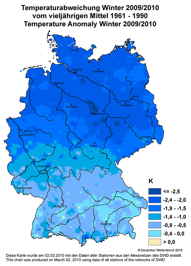
Figure 1 Temperature anomaly in winter 2009/10 with respect to the multi-year average from 1961 to 1990. Figure created by Deutscher Wetterdienst (German weather service, DWD) and downloaded from https://www.dwd.de/EN/ourservices/klimakartendeutschland/klimakartendeutschland.html?nn=495490 (last access: 1 April 2022).

3 Method

Data-driven machine learning applications require substantial effort to select and preprocess the data to be used. In the case of environmental data, researchers have to find a compromise between available data and the independence of data used for training, validation and testing, mostly due to limitations in data availability (Schultz et al., 2021). To incorporate the information from one or three upstream wind sectors, the preprocessing of data had to be expanded compared to Kleinert et al. (2021) and is presented in Sect. 3.1. Moreover, we briefly introduce the MLAir framework (Leufen et al., 2021), which we have used to carry out the experiments (Sect. 3.2), and the model architecture and training procedure (Sect. 3.3).

3.1 Data preprocessing

The main focus of this study is to assess the added value of incorporating upstream information in the sense of a chemical air parcel history on the characteristics of air quality, i.e. ozone, forecasts with a deep neural network. For this, we define three sets of experiments: firstly, a baseline (NNb) experiment with no upstream information, secondly, a single sector (NN1s) and thirdly a multi-sector (NN3s) approach. These sets of experiments necessitate different preprocessing steps, which we introduce in the following (see also Table 3 for a summary of acronyms). As the ultimate goal of our experiments and methods is to apply them to air quality observations, we selected the locations of German air quality stations as our input and target data and applied nearest-neighbour sampling to extract the specific WRF-Chem model grid box “representing” the location of a given measurement site. From here on, we will refer to those grid boxes as pseudo-observations and pseudo-measurement stations.

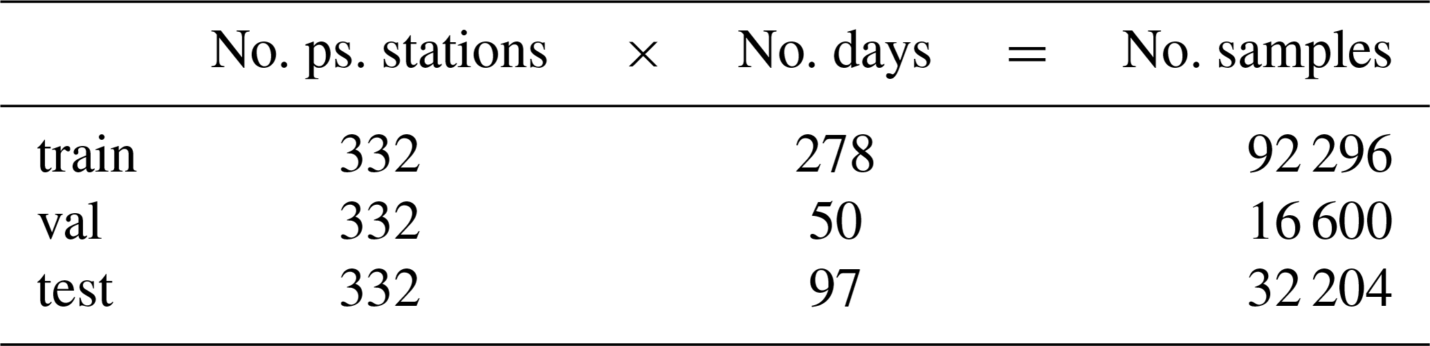
All in all, we use data from 332 pseudo-measurement stations for training, validation and testing of the neural network by following Kleinert et al. (2021). Thereby, 247 grid boxes contain exactly one, 35 grid boxes contain two and five grid boxes contain three pseudo-stations, respectively. As Schultz et al. (2021) and Kleinert et al. (2021) propose, we use a consecutive data split. We train the model with data ranging from 1 January to 15 October 2009 and use a short validation period ranging from 16 October to 14 December 2009. The final test period, which we used for all results presented below, covers 16 December 2009 to 31 March 2010. This split is motivated by the fact that ozone concentrations during winter are primarily determined by transport processes as opposed to summertime, when photochemistry plays a more active role. Hence, the effects of incorporating upstream information should become more apparent if we evaluate (i.e. “test”) our model for winter months (DJF(M)). However, the model is trained with data from all seasons and thus needs to generalise sufficiently well to capture the strong seasonal cycle of ozone concentrations. An overview of our data split is shown in Fig. 2 and Table 1.

Table 1 Number of pseudo-stations and number of samples for the training (train), validation (val) and testing (test) data sets.

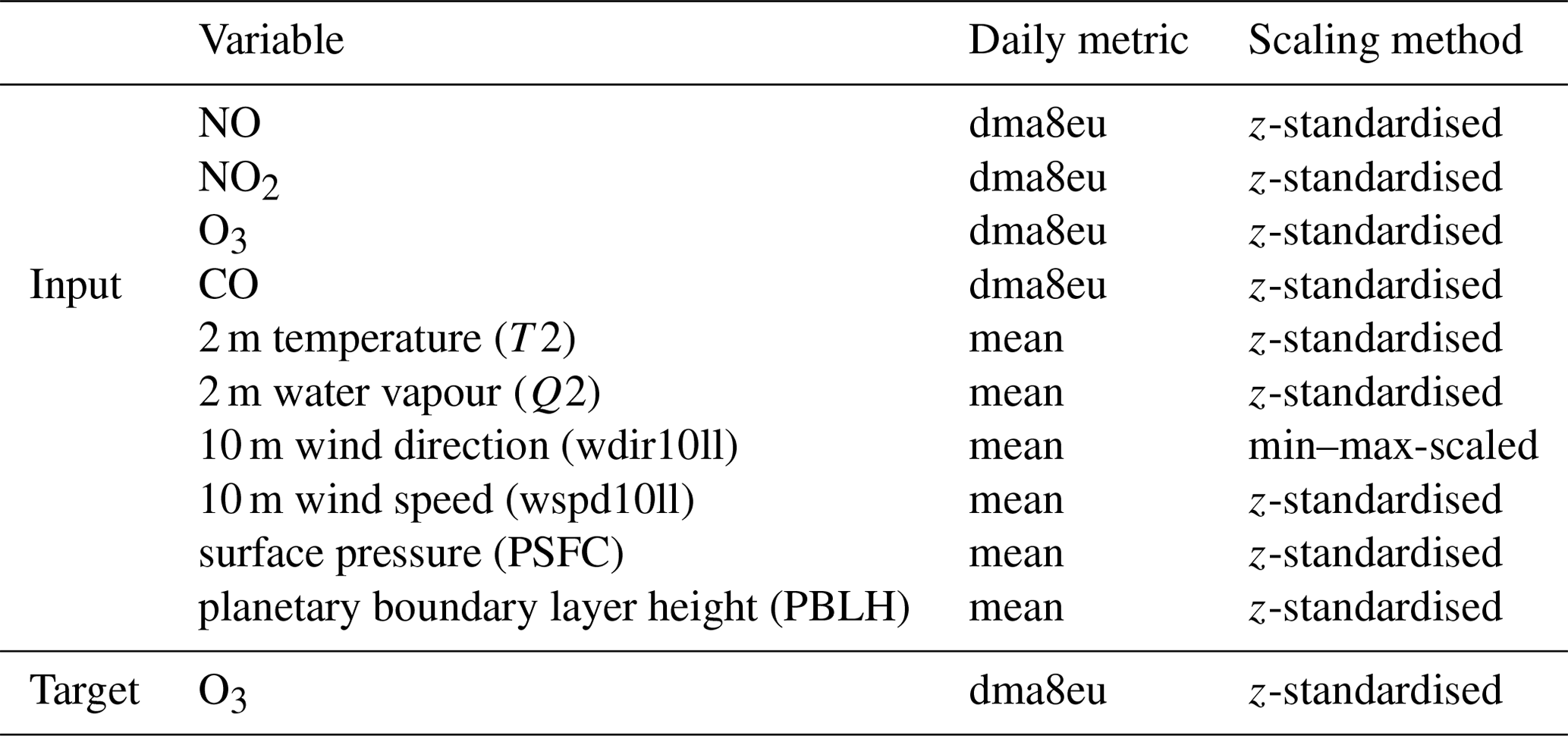
We use the following meteorological variables as model input (X): 2 m temperature (T2), 2 m water vapour mixing ratio (Q2), surface pressure (PSFC), planetary boundary layer height (PBLH), 10 m horizontal wind speed (wspd10ll) and 10 m wind direction (wdir10ll). We convert the horizontal wind components from the Lambert conformal conic projection of WRF-Chem to the geographic coordinate system. We further convert the winds' u and v component to wind speed and wind direction to determine the upstream wind direction. Moreover, we use the following chemical variables from the lowest model level: ozone (O₃), nitrogen oxide (NO), nitrogen dioxide (NO₂) and carbon monoxide (CO). We aggregate the hourly model values to daily means (meteorological variables) and maximum daily 8 h means (dma8eu) (chemical variables¹; see also Table 2) according to the EU definitions (European Parliament, 2008) using the toarstats Python package (Selke et al., 2021). Afterwards, we z-standardise all data from the training set except the wind direction to mean zero with unit variance. The wind direction is min–max-scaled. Subsequently, we apply the scaling parameters obtained from the training set to the validation and testing data sets. This approach allows for the most rigorous evaluation of the model's generalisation capability because no implicit information of the validation and testing sets contaminates the training set. Table 2 summarises all variables, their aggregated statistics and the applied scaling method.

Table 2 Input and target variables with applied daily aggregation and scaling method.

For the baseline experiment (NNb), we take the daily meteorological and chemical variables (see also Sect. 2) at a pseudo-measurement station of the previous N=6 time steps (t₋₆ to t₀) to create the input tensor (X) for our neural network. Accordingly, we use the next M=4 time steps (t₁ to t₄) at the same pseudo-measurement station to create the labels (y). We repeat this procedure for all K=332 pseudo-measurement stations.

For NN1s and NN3s we use additional chemical and meteorological information of the surrounding area as inputs to the neural network. We divide the wind directions into eight sectors corresponding to (i) north, (ii) north-east, (iii) east, (iv) south-east, (v) south, (vi) south-west, (vii) west and (viii) north-west. Consequently, each section covers 45^∘. For each of our pseudo-observations, we identify the upstream wind sector at time t₀. We then select all WRF grid boxes (centre points) which fall into this sector and have a maximal distance of 200 km to the central point of interest. Next, we compute the spatial mean for all chemical and meteorological variables in this set of grid boxes and use this aggregated information as additional input on top of the local pseudo-observational input that is used in NNb. For NN3s experiments, the same processing is applied to data in the sectors to the left and right of the upstream wind sector. Algorithm 1 depicts the preprocessing strategy.

Figure 3 shows the distribution of upstream sectors, i.e. number of samples, within the test set. The south-western sector dominates (∼ 8200 samples), followed by the western sector (∼ 4800 samples). The northern and north-western sectors contain fewer than 2000 samples each.

Algorithm 1 Data preprocessing: NNb, NN1s, NN3s.

1:

Apply toar_stats to all variables

2:

Convert horizontal wind components from Lambert conformal to geographic coordinate system

3:

Rescale time series with parameters from training set

4:

for all Pseudo-stations: Create samples do

5:

Identify grid box representing pseudo-station

6:

if NN1s or NN3s then

7:

detect upstream wind sector at t₀

8:

average across all grid boxes within the sector

9:

if NN3s then

10:

detect “left” and “right” upstream wind sector at t₀

11:

average across all grid boxes within each sector

12:

end if

13:

end if

14:

Create inputs X with variables of 7 d (−6 d) to (0 d)).

# Shape of X: $\mathrm{7}\times \mathrm{1}\times (\mathrm{10}+\mathrm{10}s)$: number of days, 1, number of pseudo-measurement variables + aggregated sector variables

# s(NNb) = 0, s(NN1s) = 1, s(NN3s) = 3

15:

Create labels y with ozone (dma8eu) concentrations for the next 4 d (1 to 4 d).

# Shape of y: 1×4 (1, lead time)

16:

end for

17:

Permute samples in the training set

18:

Create batches of size 256

Figure 2 Data availability and split into training (orange), validation (green) and testing (blue) data sets. Each day contains data from all 332 pseudo-stations.

Figure 3 Number of samples per (main) upstream wind sector at time step t₀ within the testing set.

3.2 MLAir framework

We use the Machine Learning on Air data (MLAir, version 1.5) framework (Leufen et al., 2021) as the backbone for our experiments. MLAir provides a workflow framework for machine-learning-based atmospheric forecasts with easily extensible modules for data preprocessing, training, hyperparameter optimisation and evaluation. MLAir uses the TensorFlow (Abadi et al., 2015), dask (Rocklin, 2015) and xarray (Hoyer and Hamman, 2017) libraries. For each of the mentioned preprocessing methods (see Sect. 3.1), we implemented individual DataHandlers (see Leufen et al., 2021, Sect. 2.5) that allow us to modify the data preprocessing steps while maintaining the same training and evaluation procedures for all experiments in spite of the different data structures.

3.3 Model architecture and training procedure

In contrast to our previous study (Kleinert et al., 2021), we use a U-shaped convolutional neural network (CNN) with two parallel long short-term memory (LSTM) cells in the lowest level. Ronneberger et al. (2015) first introduced the U-Net architecture for biomedical image segmentation, but many other disciplines picked up this architecture. U-shaped or U-Net architectures have already been used to successfully tackle spatio-temporal problems (He et al., 2022). As outlined in Sect. 3.1, we train three different models according to the three preprocessing variants: (i) baseline (NNb), (ii) one upstream sector (NN1s) and (iii) three upstream sectors (NN3s). The model architecture for the NN3s model is shown in Fig. 4. The first layer is the input layer. During training the individual samples in X, representing short 7 d time series (t₋₆ to t₀) for each variable, are passed to the network. We use the variables as channel dimension. We use 2D convolutional layers with a degenerated width dimension. Thus, the overall dimension of our training set is no. $\text{samples}\times \text{prev. }N\text{ days}\times \mathrm{1}\times$ no. (sector) variables. We use a kernel size of 3×1 for convolutions and a pooling kernel size of 2×1. We apply exponential linear units (ELUs; Clevert et al., 2016) as an activation function for inner layers and a linear activation function for the output layer. Due to the different input data structures between the three experiment sets, the model architectures differ from each other in terms of the number of channels. Other design parameters – like the number of layers and kernel sizes – are identical across all runs. As the time series are relatively short, we use symmetric padding to ensure that the temporal dimension does not shrink. In the U structure's lowest level, we use two LSTM branches after the third convolution block. While we used a max-pooling layer before the first LSTM branch to capture highly dominant features, the second LSTM branch uses the whole temporal dimension of size seven. We use an upsampling layer to expand the temporal dimension of the first LSTM branch and concatenate the resulting tensor with the symmetric padded skip connection of the third convolution block. We apply an additional convolutional layer for information compression before we append (concatenate) the second LSTM branch. Afterwards, we use altering concatenation and convolution layers to reconstruct the U's right slope. Finally, we use a simple dense layer with four nodes as the output layer. Here each node corresponds to the prediction for time step t₁ to t₄.

The original U-Net proposed by Ronneberger et al. (2015) does not include padding as their input images are large enough for multiple convolutions. For each convolutional operation with a kernel size of k, the processed input data's shape shrinks by k−1 (assuming no padding and strides s=1). To prevent the inputs from becoming too small, we implement the paddings mentioned and use the standard UpConv layer after the unpadded LSTM branch only. We train all models for 300 epochs using Adam (Kingma and Ba, 2014) as the optimiser and the mean squared error as the loss function. Detailed information on the choice of hyperparameters can be found in Table A1.

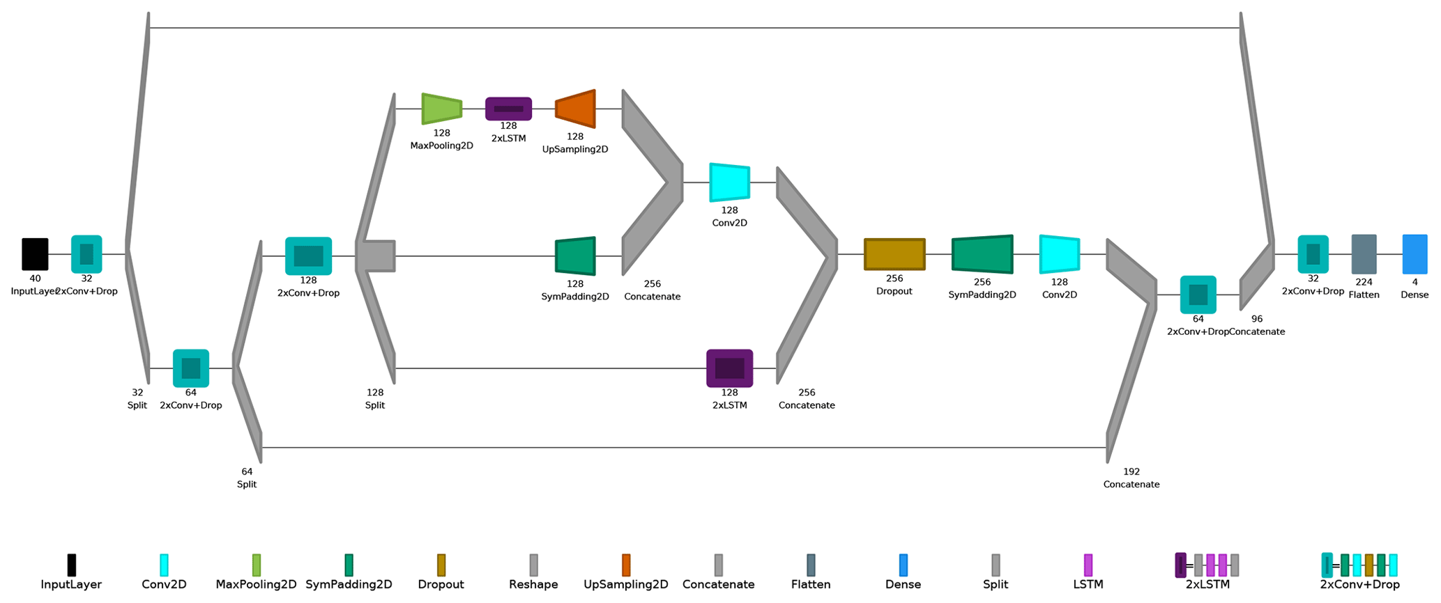
Figure 4 Summary of NN3s model architecture with input (black, left), hidden, and output (blue, right) layer. Several layers are grouped for better visualisations. Colour-coding of individual layers and groups is shown on the right. This figure was created with Net2Vis (Bauerle et al., 2021).

3.4 Reference models

As in Kleinert et al. (2021), we use persistence and an ordinary least-squares (OLS) model as references to provide a meaningful baseline evaluation of our machine learning models. The persistence forecast is built simply using the latest observation at t₀ as forecast for all lead times t₁ to t₄. The persistence model serves as a relatively strong competitor on short lead times and should be outperformed by all other models which add any value to the forecasting solution. To train the OLS model, we use the same data set as for the NN3s network. The OLS model serves as a linear competitor and therefore as an indicator on how well the neural networks differ from a “simple” linear forecast. A detailed description of these two reference forecasts is provided in Leufen et al. (2021) (MLAir) and Kleinert et al. (2021) (IntelliO3-ts). We also reran the experiments from this study with the IntelliO3-ts (Kleinert et al., 2021) model architecture, which is based on inception layers (Szegedy et al., 2015), for comparison. As described in Sect. 3.1, three different variants of the IntelliO3 architecture had to be built because of the different input data dimensions. All models were trained from scratch using the same data as in our main experiments.

Table 3 summarises the experiments described in this paper and introduces the labels that are used to denote these experiments in the Results section.

Table 3 Naming of deep learning experiments and reference models described in this paper.

4 Results

We first present the results of the two sectorial approaches (NN1s and NN3s) in comparison to the baseline method (NNb), which does not use any upstream information. These three models are compared to OLS, persistence and the IntelliO3_[b, 1s, 3s] variants. Secondly, we compare the individual losses of NN3s based on the training, validation and testing loss. Afterwards, we present more detailed results for the multi-sector approach (NN3s), including an exemplary sensitivity analysis for input variables.

Figure 5 shows the overall mean squared error (MSE) for all models and reference models across all lead times. We can clearly distinguish between different experiments (p<0.001; see below). The U-Net architecture networks (NN3s, NN1s, and NNb) show the lowest root mean square error (RMSE). Conversely, the multi-sector, baseline IntelliO3 and persistence experiments (IntelliO3_3s, IntelliO3_b and persi) show the largest RMSE. We estimate the uncertainty by performing a block-wise bootstrapping with a block length of 7 d and 1000 draws with replacement. Additionally, we perform a non-parametric two-sided Mann–Whitney u test (5 % significance level) for NN3s and all competitors.

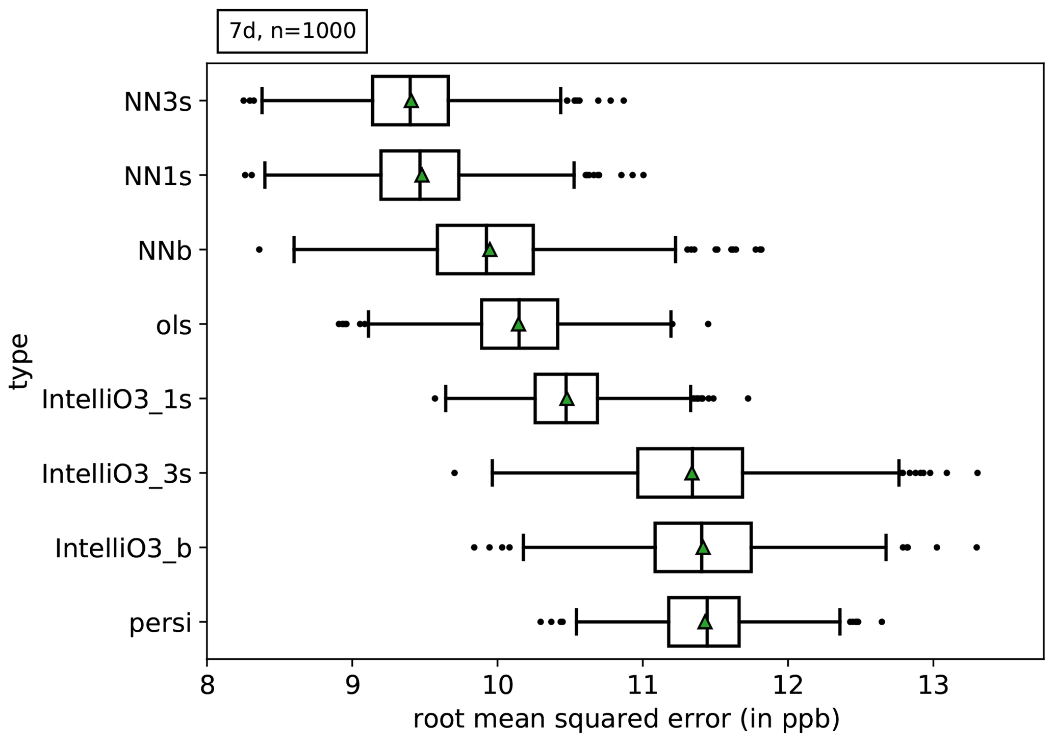
Figure 5 Estimated uncertainty of the mean squared error using block-wise bootstrapping (1000 realisations with replacement with block length of 7 d). IntelliO3_* corresponds to the model architecture as presented in Kleinert et al. (2021) (IntelliO3-ts v1.0).

The NN3s approach shows the lowest RMSE, and the null hypothesis of the performed u test can be rejected (p<0.001) for all competitors (detailed test statistics and corresponding p values are shown in Appendix Table B1). NN3s performs better than the baseline (NNb) and the single sector (NN1s) approach, which in turn exhibits a lower RMSE compared to OLS, the InitelliO3 variants and persistence.

Figure 6 shows a monthly comparison of the forecast distributions per lead time for the pseudo-observation. The results are shown for the test data set period ranging from December 2009 to March 2010 (see also Sect. 3.1). The forecasts show a narrower distribution when compared to the pseudo-observations' distribution. While we can observe that the NN3s model captures the changing monthly structure in terms of varying mean and median concentrations, the network is not able to adequately reproduce the variability and forecasts converging towards the monthly means. Such a behaviour was already found in Kleinert et al. (2021).

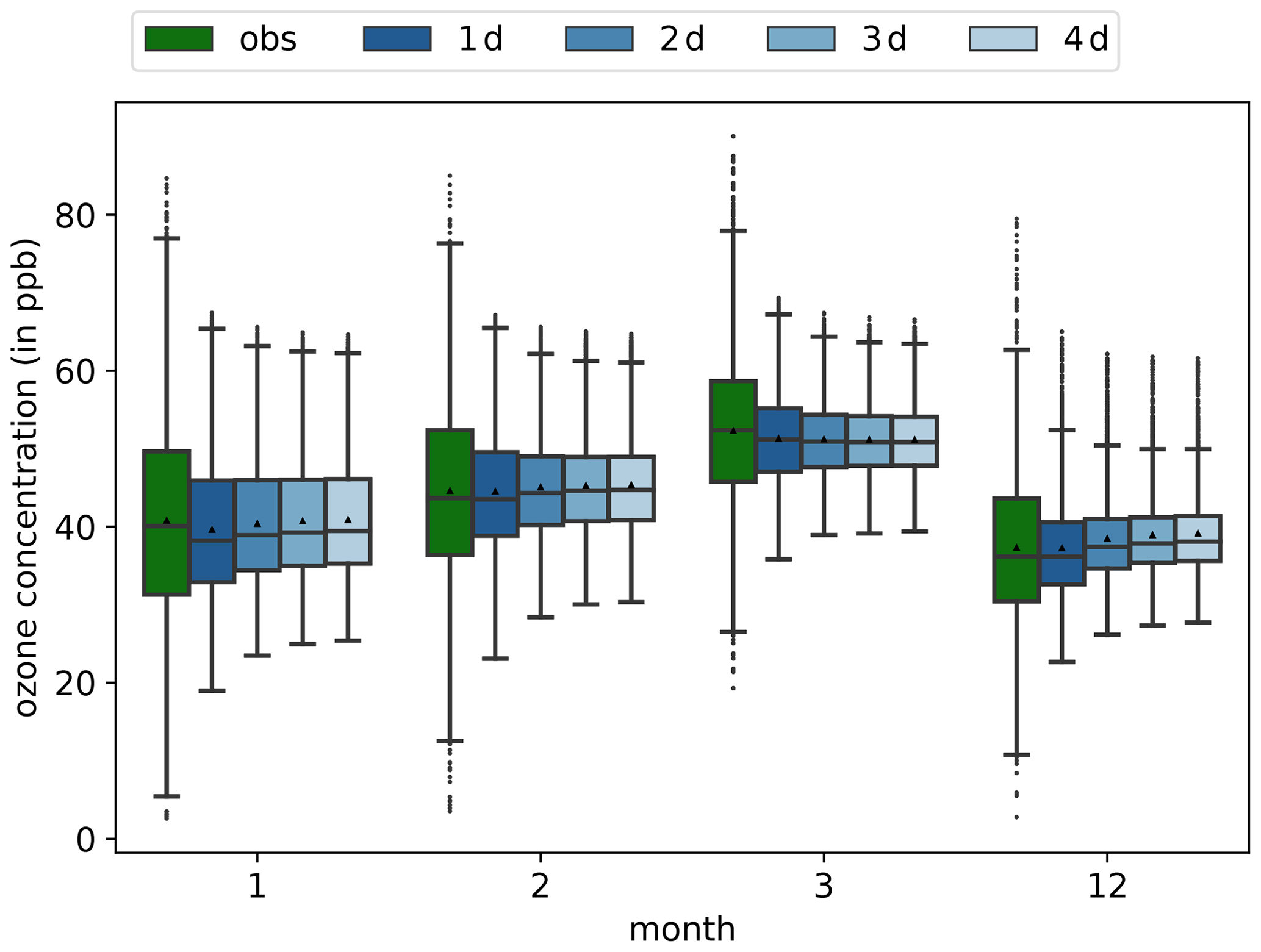
Figure 6 Monthly dma8eu ozone concentration for all test pseudo-stations as box plots. Pseudo-observations are denoted by obs (green), and forecasts are denoted by 1 d (dark blue) to 4 d (light blue). Triangles display the arithmetic means.

More insights can be gained from evaluating the skill scores of the various experiments for the individual lead times (i.e. 1 d to 2 d). As we base the comparison of our models on the mean squared error (MSE), the skill scores (S) take the form of

$$\begin{array}{}\text{(1)}& S\left(\mathit{m},\mathit{r},\mathit{o}\right)=\mathrm{1}-{\displaystyle \frac{\mathrm{MSE}\left(\mathit{m},\mathit{o}\right)}{\mathrm{MSE}\left(\mathit{r},\mathit{o}\right)}},\end{array}$$

where m is a vector containing the model's forecast, o is a vector containing the corresponding observations and r is a vector containing the reference forecast (Murphy, 1988). Here a positive value of S>0 corresponds to an improvement of the model over the reference. Consequently, a negative value (S<0) corresponds to a deterioration of skill with respect to the reference forecast.

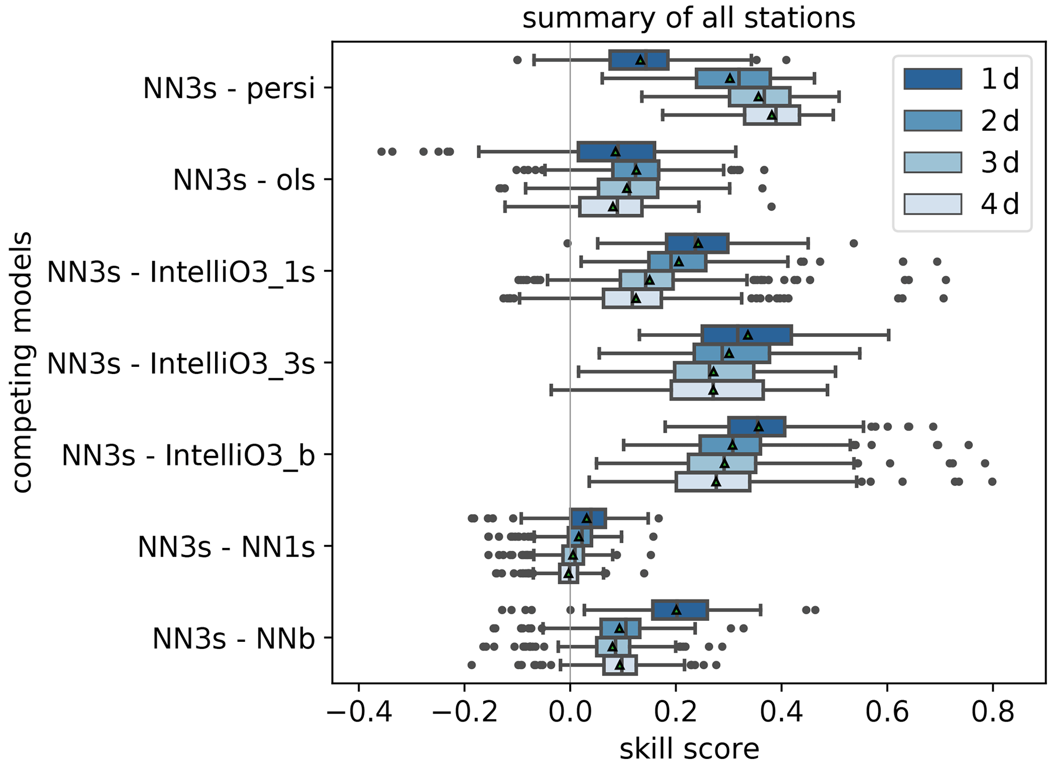
Figure 7 Skill scores of the NN3s model versus the reference models persistence (persi), ordinary least-squares (ols), single upstream sector model (NN1s) and pseudo-station model (NNb) based on the mean squared error, separated for all lead times (1 d (dark blue) to 4 d (light blue)). Positive values denote that NN3s performs better than the given references. Triangles display the arithmetic means.

Figure 7 shows the skill scores separated for all lead times. Here the uncertainties (boxes and whiskers) are calculated based on the individual pseudo-stations. As expected, the NN3s approach shows an increasing skill score with increasing lead time when the persistence forecast is used as reference (mean from ∼0.13 on 1 d to ∼0.38 on 4 d). When we compare NN3s with respect to the OLS model, the mean skill score is positive throughout (overall mean ∼0.10) and has its maximum for a lead time of 2 d (mean ∼0.13), with the smallest interquartile range (IQR). For 3 and 4 d lead times, the skill score decreases. For the comparison of NN3s with respect to the IntelliO3 variants (_b, _1s _3s), we can observe a general pattern with the highest skill score on 1 d, which decreases with increasing lead time. The mean skill score of NN3s vs. IntelliO3_3s decreases from ∼0.34 to ∼0.27, NN3s vs. IntelliO3_1s decreases from ∼0.24 to ∼0.12 and NN3s vs. IntelliO3_b from ∼0.35 to ∼0.26, respectively. The additional two upstream sectors of IntelliO3_3s do not add any additional information compared to its single sector approach (IntelliO3_1s).

Even though NN3s provides a significant performance improvement over NN1s as shown in Fig. 5, the skill score of the NN3s vs. NN1s comparison is close to zero during all 4 forecast days (mean ∼0.03 on 1 d, ∼0.02 on 2 d, ∼0.01 on 3 d and ∼0.0 on 4 d). The added value of neighbouring upstream sectors is apparently lost after 1 d.

For the comparison of NN3s with respect to NNb, we see the largest skill score for a lead time of 1 d (mean ∼0.2) which decreases up to 3 d (∼0.09, ∼0.08) and slightly increases again at 4 d (∼0.09).

As we originally expected a greater benefit of using upstream wind sector information for ozone forecasts, we have further analysed these skill scores and looked at their spatial distribution. From Fig. 7 we can identify some pseudo-stations for which the ols model performs better then the NN3s model. To capture potential differences in spatial properties, Fig. 8 shows the skill NN3s vs. ols skill scores for each pseudo-station. The skill score (NN3s vs. ols) is mostly positive in the northern part of Germany on 1 d and is mostly negative in mountainous regions in the south of Germany. With increasing lead time, the skill score also becomes positive in the mountainous regions but tends to turn negative in the north-east.

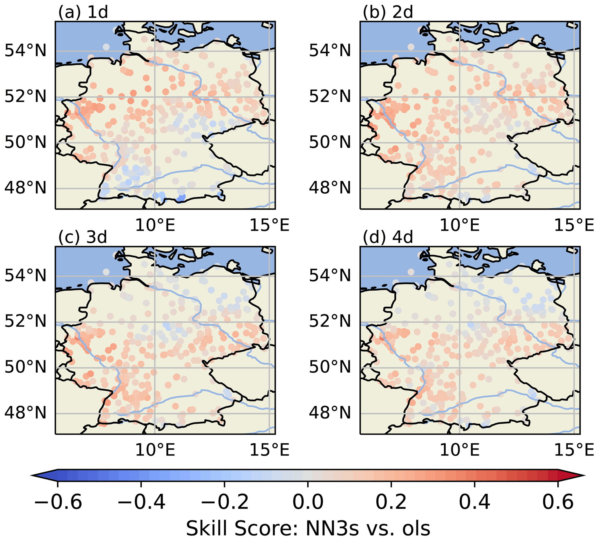
Figure 8 Skill score (NN3s vs. ols) per station for lead times of 1 d (a) to 4 d (d). This figure was created with Cartopy (Met Office, 2010–2015). Map data © OpenStreetMap contributors 2022. Distributed under the Open Data Commons Open Database License (ODbL) v1.0.

5 Discussion

Based on the results presented in Sect. 4, we can observe that NN3s outperforms the (simplistic) persistence and OLS forecasts as well as NNb, which only uses the pseudo-observations of a specific grid box. The increase of the NN3s-persi skill score with increasing lead time (Fig. 7) is in line with expected behaviour as the persistence forecast has its most valuable predictions for short lead times. Consequently, the increased skill score for NN3s-persi is mostly caused by the worsening of the persistence forecast with increasing lead time. However, the positive skill score for a lead time of 1 d shows that the NN3s model has a genuine added value over the persistence forecast on short lead times. When comparing NN3s and NN1s, we see that the skill score's lower bound of the IQR is close to zero for the first 2 d of prediction and that the skill score's mean and median converge towards zero for the remaining lead times, meaning that NN3s behaves like NN1s for 3 and 4 d. Consequently, NN3s can not extract any additional helpful information from the input fields for 3 and 4 d. Most likely, this effect is caused by the definition of neighbouring sectors as described in Sect. 3.1, where we use the upstream wind sector and the two adjacent sectors with a radius of 200 km at time step t₀ to calculate the spatial means for all input time steps t₋₆ to t₀. Thus, depending on the average wind speed, the static upstream wind sectors cannot provide all relevant information. Moreover, the sectorial approach is a cruder approximation of a streamline than a backwards trajectory, and differences between both of them tend to increase with increasing lead time. Based on the NN3s and NN1s sample uncertainty estimate in Fig. 5 and the competitive skill score per lead time in Fig. 7 we can conclude that the statistical significance of the u test (Appendix Table B1) is related to the better performance on the first two lead times (1 and 2 d).

In the following, we discuss differences in the training, validation and testing loss of NN3s, the influence of the upstream wind direction and implications based on our data split in more detail.

5.1 Evaluation of training, validation and testing differences

We use different parts of a year to train, validate and test our models (see Sect. 3.1). Consequently, the network encounters different meteorological and chemical conditions. Therefore, we compare the differences in the MSE (which we used as the loss function during training) for the training, validation and testing sets for each station individually. Averaged over all stations, the mean rescaled losses for NN3s are 64.08 ppb² (train, scaled: 1.04), 63.34 ppb² (val, scaled: 0.98) and 64.62 ppb² (test, scaled: 1.08). Figure 9 shows how the losses are distributed geographically. At first glance, we can identify regions with high MSE (>120 ppb², yellowish colours) in the mountainous south and in the northern coastal area. The triangles denote the losses of each station separated for the training (left part of the symbol), validation (right part of the symbol) and test (lower part of the symbol) set. When focussing on the set's loss differences at individual pseudo-stations, we can identify the following pattern: the test set's loss is mostly lower than the validation and train loss in Germany's western and south-western parts. The high individual validation loss in the northern part is directly related to the large temperature anomaly, as shown in Fig. 1. Thus, the feature combination is not explicitly present in the training set, resulting in larger discrepancies in forecasts and observations.

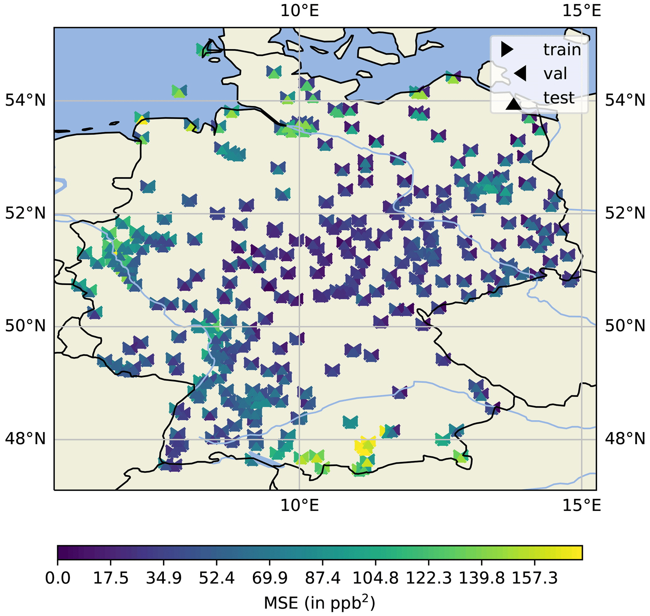
Figure 9 MSE of the training (left triangle), validation (right triangle) and testing (bottom triangle) data sets for each station. This figure was created with Cartopy (Met Office, 2010–2015). Map data © OpenStreetMap contributors 2022. Distributed under the Open Data Commons Open Database License (ODbL) v1.0.

5.2 Sectorial results – NN3s

In the following we further analyse the influence of the upstream wind direction on the skill score. As mentioned in Sect. 2, the SW direction is the dominant upstream sector in the testing set, while the fewest cases are found in the NW sector.

Figure 10 shows the skill score separated for each wind sector (NN3s vs. NNb). We can observe that the skill score is mostly negative for the northern sector ($\sim -\mathrm{0.2}$), having a low number of samples (Fig. 3). On the contrary, the south-western sector's skill score is – on average – positive but close to zero, indicating that NNb performs equally well in the dominant upstream direction. On average the skill scores for E, SE, S and W are positive, indicating that the NN3s model can extract some useful information in contrast to using the pseudo-observation at the pseudo-location only. However, it also becomes obvious that this is not the case for all stations (negative skill scores indicated by dots). It seems that the additional information provided by the upstream sectors might sometimes confuse the network and therefore does not have the desired effect at all instances.

Figure 10 Skill scores (NN3s vs. NNb) based on the upstream wind direction at time step t₀.

5.3 Non-linearities

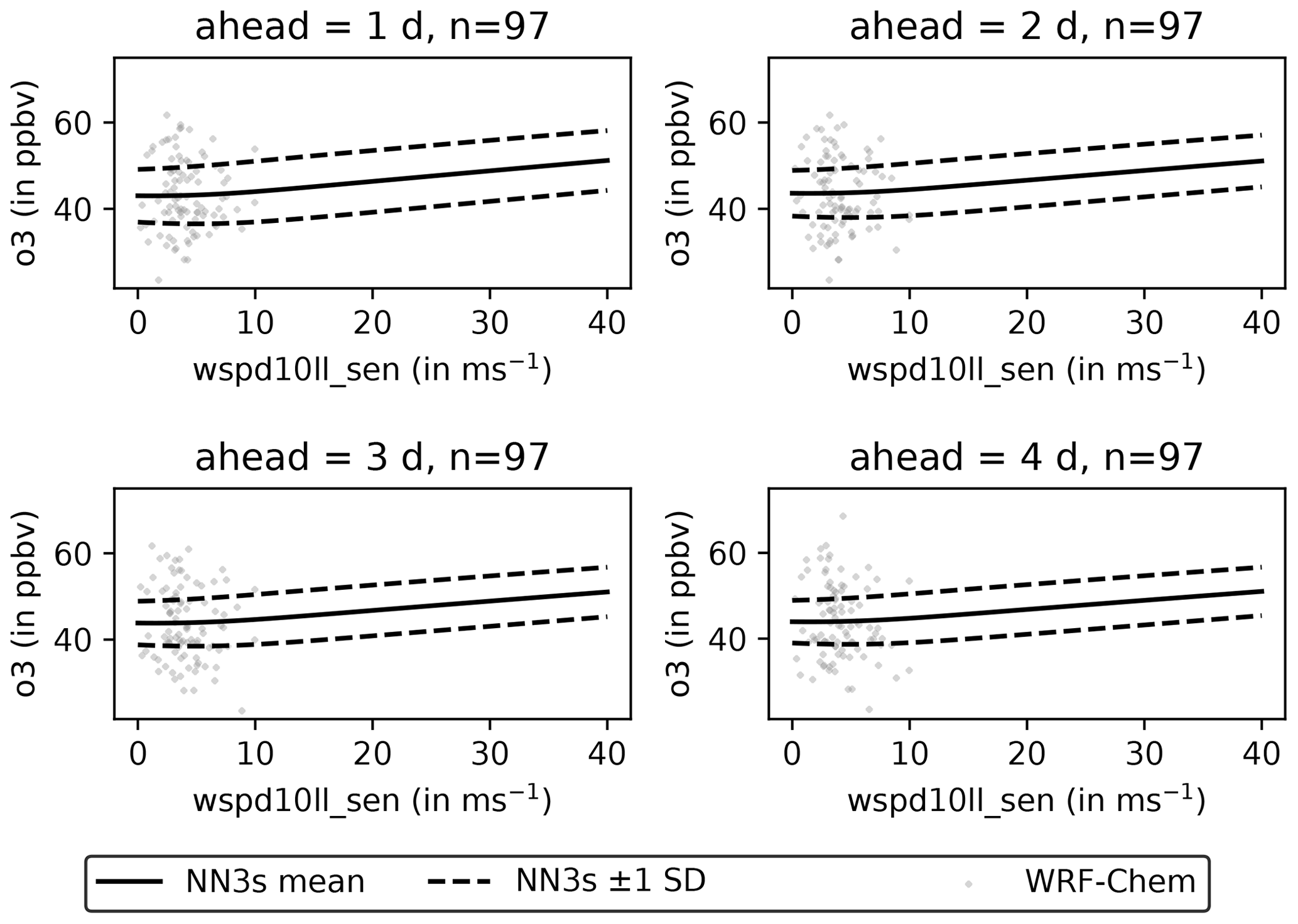
As we saw in Fig. 8, there are pseudo-stations in Germany, where a simpler OLS model produces a better forecast than NN3s. Naively, one might expect a neural network to generate better forecasts because of its ability to capture non-linear dependencies between variables. To better understand these non-linearities, we iteratively modify the input variables of each sample (in all sectors and the pseudo-observation). Afterwards, we feed the modified input samples into the trained NN3s model and detect how the ozone forecasts for all lead times change. Figure 11 shows the sensitivity of ozone inputs for one example station. For the O₃ sensitivity test, the resulting sample distribution is very narrow. We can identify two regions from 0 to ∼ 50 ppb and from 80 ppb to the maximum value of 170 ppb, with a transition region in between. The shallower increase in the second region aligns with the findings from Fig. 6, where we see that NN3s cannot adequately reproduce high ozone levels. Figure 12 shows the sensitivity towards 10 m wind speed. The wind speed analysis results in a broader distribution with a flat shape from 0 to 10 m s⁻¹ and a linear increase for larger wind speeds.

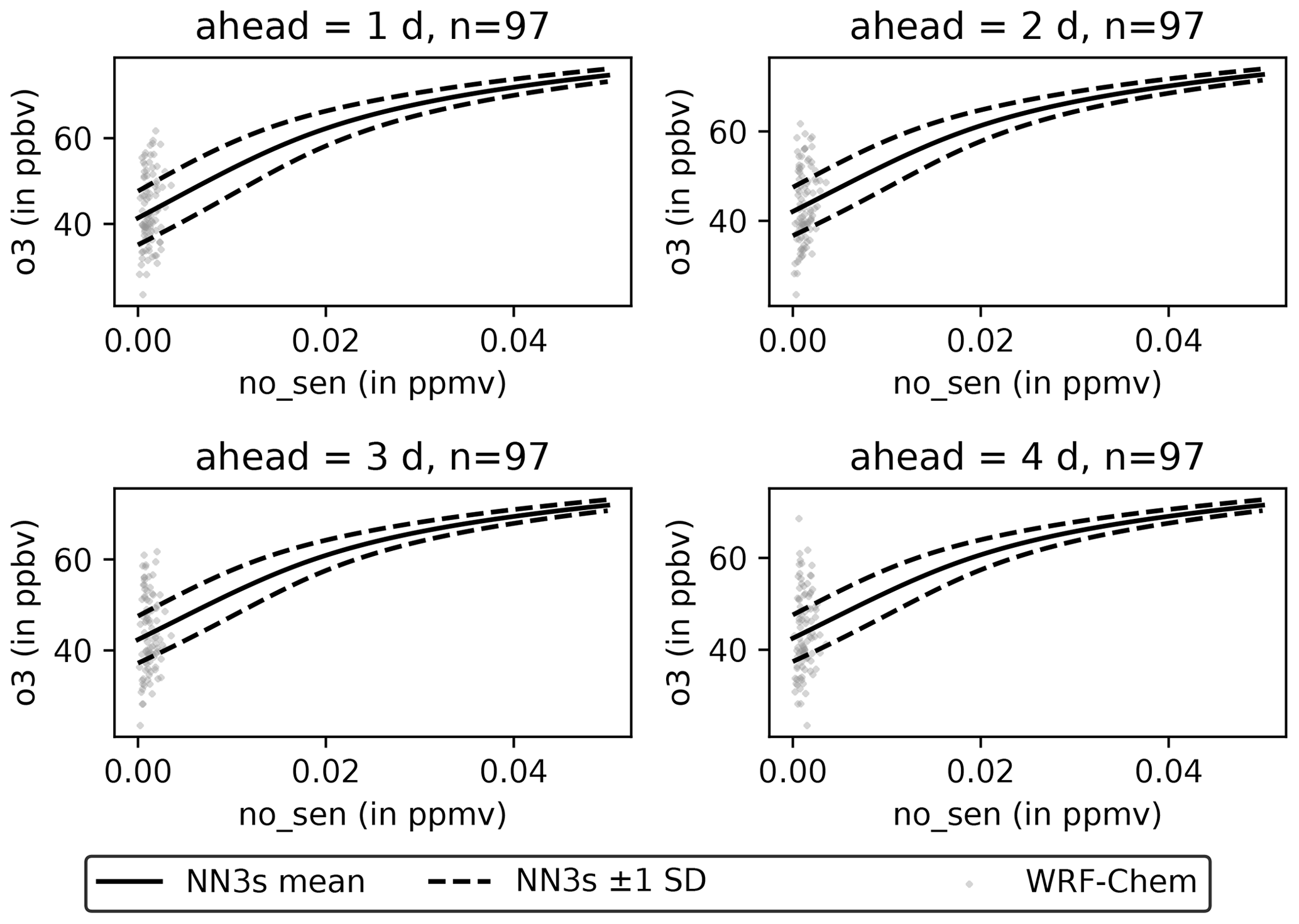
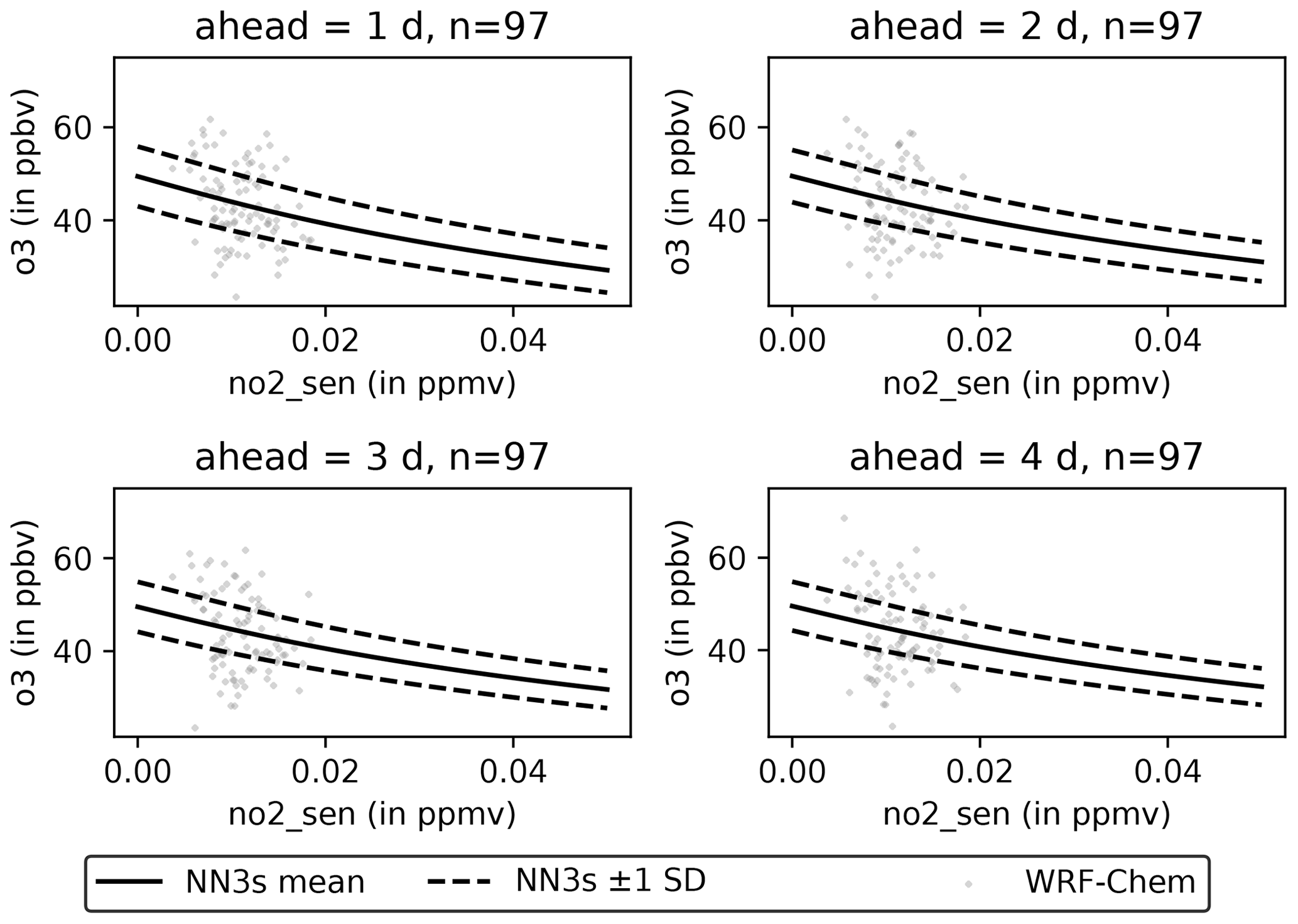
An increase of NO levels leads to an increase of the resulting ozone level (Fig. 13). The increase is strongest for low NO levels and flattens for larger NO levels. Conversely, an increase on NO₂ leads to a decrease of the resulting ozone levels (Fig. 14) forecasted by NN3s.

Disentangling the influences of NO_x and volatile organic compound (VOC) species on ozone concentrations is a complex endeavour. Investigations into these relations with CTMs show that the results depend on the details of the chemical mechanisms as well as other model parameterisations (e.g. for deposition or biogenic VOC emissions). Fast et al. (2014) showed that the reduction of all anthropogenic emissions by 50 % only has a relatively minor effect on the O₃ bias in California, with differences of up to ∼5 ppb at four selected sites compared to a simulation with default emissions. Abdi‐Oskouei et al. (2020) performed several sensitivity studies to assess the impact of meteorological boundary conditions and the land surface model on modelled O₃ concentrations, and they showed that these changes led to a minor sensitivity of average ozone concentration (<2 ppb). Georgiou et al. (2018) analysed the impact of the different chemical schemes on predicted trace gases and aerosol concentrations, and they found that CBMZ-MOSAIC and MOZART-MOSAIC have similar O₃ biases (10.9 and 11.6 ppb), while the use of the RADM2-MADE/SORGAM mechanism led to a smaller bias of 4.25 ppb. These differences were attributed to the difference in VOC treatment. Gupta and Mohan (2015) have also analysed the sensitivity of ozone concentrations to the choice of the chemical mechanism and noted that the CBMZ performed better than the RACM mechanism due to the revised rates of inorganic reactions in the CBMZ mechanism. Mar et al. (2016) found that the absolute concentration of ozone predicted by the MOZART-4 chemical mechanism is up to 20 µg m⁻³ greater than RADM2 in summer. This is explained by the different representations of VOC chemistry and different inorganic rate coefficients. Liu et al. (2022) developed a deep learning model for correcting O₃ biases in a global chemistry–climate model and demonstrated that temperature and geographic variables showed the strongest interaction with O₃ biases in their model.

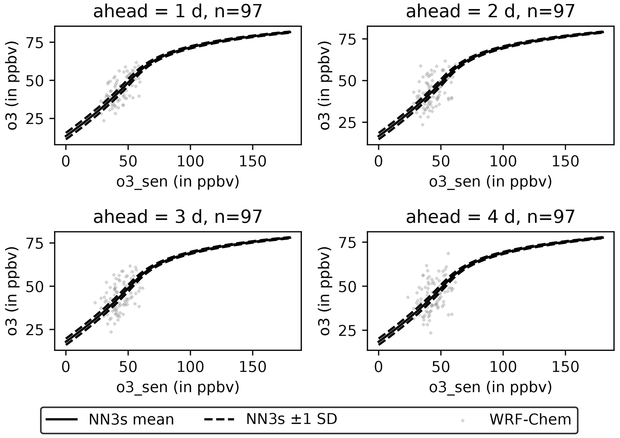
Figure 11 Sensitivity of NN3s forecasts for an exemplary station located at 50.770382^∘ N and 9.459403^∘ E with respect to ozone. Light grey dots (97) represent each sample's daily aggregated WRF-Chem values at time step t₀. The solid black line represents the mean sensitivity across all samples, and the dashed black lines represent ± 1 standard deviation, respectively. Sensitivities are shown individually for all lead times (1 to 4 d).

Figure 12 Same as Fig. 11 but for 10 m wind speed instead of ozone input.

Figure 13 Same as Fig. 11 but for NO instead of ozone input.

Figure 14 Same as Fig. 11 but for NO₂ instead of ozone input.

5.4 Concept drift

We trained all our models and reference models with data ranging from 1 January to 15 October 2009. We selected a short validation period from mid-autumn to early winter and finally based our analysis on data from the winter and early spring seasons. Thus, as depicted in Fig. 1 the testing set contains data from an unusually cold winter, which was not reflected adequately in the training set. Therefore, the network encounters some input patterns and combinations of features during testing, which are not similar to any data used for training, and thus the DL network has to generate predictions outside of its “comfort zone” (see, for example, Leonard et al., 1992, and Pastore and Carnini, 2021, or Ziyin et al., 2020, for periodic data). As presented in Sect. 2, the temperature anomaly during winter 2009/10 was largest in northern Germany and less, but still negative, in the southern parts of Germany. We can observe a similar north–south pattern for the skill scores (NN3s vs ols) per station (Fig. 8) and a skill scores' change of sign with increasing lead time. Nonetheless, our analysis cannot attribute these phenomena and the geographic height to each other, and further analysis using explainable machine learning techniques like, for example, in Stadtler et al. (2022) would be required. In order to reduce the concept drift's effect, extending each data set to multiple years would be beneficial in upcoming studies. This would allow the network to operate on more robust data distributions and thus minimise the risk of out-of-sample predictions.

5.5 Alternative neural network approaches

This study indicates that the forecast quality of air pollutant concentrations can be increased by taking into account the spatial patterns of the meteorological and chemical fields. While our work has focused on time-series predictions to explore machine learning methods that can be trained on observational data, there are other studies which employ machine learning to forecast spatio-temporal fields. For example, Steffenel et al. (2021) used the PredRNN++ (Wang et al., 2018) model to forecast the total column ozone for the southern part of South America and parts of Antarctica. Gong et al. (2022) recently used convolutional long short-term memory models (ConvLSTM; Shi et al., 2015) and a generative Stochastic Adversarial Video Prediction (SAVP; (Lee et al., 2018)) model to forecast the 2 m temperature for a lead time of up to 12 h over Europe with some success. As a general outcome of these studies, it can be said that generative models are better suited to preserve the multi-scale structures of atmospheric fields. While the development of such models for weather applications proceeds rapidly and adopts the latest deep learning methods (see for example Pathak et al., 2022), the machine learning models for atmospheric chemistry have so far been comparatively simpler.

One option to further enhance the approach presented in this study would be the use of Lagrangian particle modelling to derive the area of influence and chemical history for observation sites (see, for example, Yu et al., 2020). Furthermore, the application of Bayesian network architectures can help to characterise data and model uncertainties in future studies (for gridded model examples, see, for example, Sengupta et al., 2020; Sun et al., 2022; Ren et al., 2022).

6 Conclusions

In this study, we explored the potential benefit of using spatially aggregated upstream information to improve point-wise predictions of near-surface ozone concentrations. Even though this analysis was based on pseudo-observations sampled from chemistry transport model, the results should apply to real observation data as well if they are not confounded by the inhomogeneous spatial distribution and missing data occurrences in observational data.

The first result from this study is that a U-Net architecture with a combination of convolutional and LSTM cells is superior to the inception block architecture presented in Kleinert et al. (2021) in this explicit forecasting setting. The second and main result is that the additional information provided by the central upstream wind sector (NN1s) improves the forecast for all lead times (1 to 4 d) with respect to the baseline model (NNb) by 10 %, which has not seen any upstream information during training. Moreover, we show that further information provided by the left and right upstream sectors (NN3s) only improves the forecasts for the first 2 d (∼ 14 %) and that there is no further improvement on the remaining days (3 and 4 d) with respect to the central upstream model (NN1s). NN3s outperforms the ols model at most of the pseudo-stations that we trained on exactly the same data. Thus, we can conclude that the non-linearity provided by the neural network is essential to extracting meaningful upstream information.

Nonetheless, we showed that the NN3s model does not outperform the ols model at all pseudo-stations and lead times. This can in part be attributed to a sampling bias because the winter in 2010 (test data) was much colder than the winter of 2009 (part of the training data). Besides these limitations, we conservatively evaluated the generalisation capability in the sense that the testing set has the largest possible “distance” to the training data. The improvement in forecast quality arising from the upstream sector information can therefore be seen as a lower limit.

The previous study of Yi et al. (2018) showed that their deep neural network model (DeepAir) that makes use of spatially aggregated information outperforms several other network architectures. In complement to their study, we investigated different preprocessing variants. Our variants use various amounts of data to encapsulate the influence on the forecasting performance of one U-shaped network type.

Appendix A: NN3s – hyperparameters

Table A1 shows the hyperparameters used to train the NN3s model. The table is automatically pooled and generated by MLAir (spelling according to TensorFlow).

Table A1 Hyperparameters used for NN3s.

Appendix B: Additional statistics

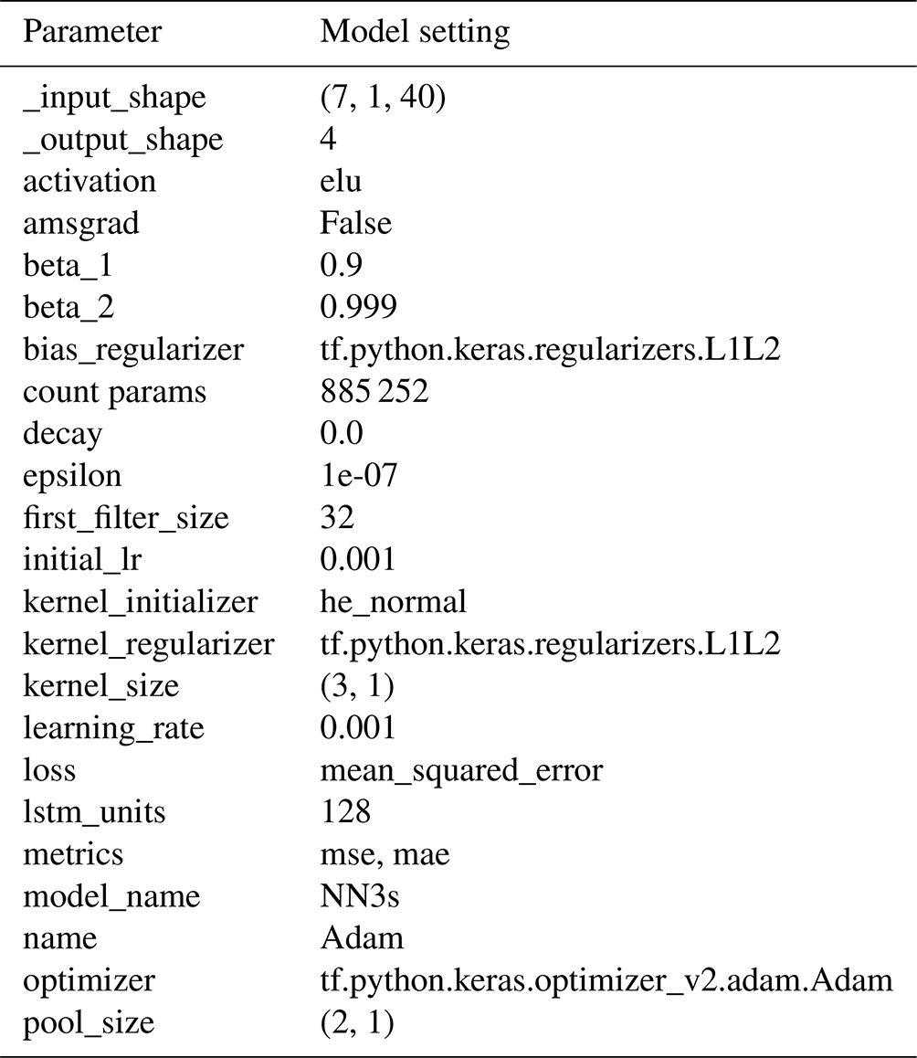
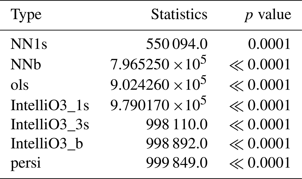
Table B1 summarises the results of two-sided Mann–Whitney u tests (5 % significance level) for NN3s and all our competitive models.

Table B1 Results of two-sided Mann–Whitney u test (5 % significance level) of NN3s and listed competitor models.