Pathfinder v1.0.1: a Bayesian-inferred simple carbon–climate model to explore climate change scenarios

The Pathfinder model was developed to fill a perceived gap within the range of existing simple climate models. Pathfinder is a compilation of existing formulations describing the climate and carbon cycle systems, chosen for their balance between mathematical simplicity and physical accuracy. The resulting model is simple enough to be used with Bayesian inference algorithms for calibration, which enables assimilation of the latest data from complex Earth system models and the IPCC sixth assessment report, as well as a yearly update based on observations of global temperature and atmospheric CO₂. The model's simplicity also enables coupling with integrated assessment models and their optimization algorithms or running the model in a backward temperature-driven fashion. In spite of this simplicity, the model accurately reproduces behaviours and results from complex models – including several uncertainty ranges – when run following standardized diagnostic experiments. Pathfinder is an open-source model, and this is its first comprehensive description.

1 Introduction

Simple climate models (SCMs) typically simulate global mean temperature change caused by either atmospheric concentration changes or anthropogenic emissions of CO₂ and other climatically active species. They are most often composed of ad hoc parametric laws that emulate the behaviour of more complex Earth system models (ESMs). The emulation allows for simulating large ensembles of experiments that would be too costly to compute with ESMs. However, the SCM denomination refers to a fairly broad range of models whose complexity can go from a couple of boxes that only emulate one part of the climate system (e.g. a global temperature impulse response function; Geoffroy et al., 2013b) to hundreds of state variables representing the different cycles of greenhouse gases and their effect on climate change (e.g. the compact Earth system model OSCAR; Gasser et al., 2017). Simpler models are easier and faster to solve, but they may not be adequate for all usages. Therefore, finding the “simplest but not simpler” model depends on a study's precise goals.

In our recent research, we have perceived a deficiency within the existing offer of SCMs, in spite of their large and growing number (Nicholls et al., 2020). We have therefore developed the Pathfinder model to fill this gap: it is a parsimonious CO₂-only model that carefully balances simplicity and accuracy of representation of physical processes. Pathfinder was designed to fulfil three key requirements: (1) the capacity to be calibrated using Bayesian inference, (2) the capacity to be coupled with integrated assessment models (IAMs), and (3) the capacity to explore a very large number of climate scenarios to narrow down those compatible with limiting climate impacts. The latter motivated the model's name.

While these three requirements clearly call for the simplest model possible, as they all need a fast solving model, they also imply a certain degree of complexity. The Bayesian calibration requires an explicit representation of the processes (i.e. the variables) that are used to constrain the model. Coupling with IAMs requires accurately embedding the latest advances of climate sciences to be policy relevant (National Academies of Sciences and Medicine, 2017). Exploring future climate impacts requires the flexibility to link additional (and potentially regional) impact variables to the core carbon–climate equations.

The Pathfinder model is essentially an integration of existing formulations, adapted to our modelling framework and goals. It is calibrated on Earth system models that contributed to the Coupled Model Intercomparison Project phase 6 (CMIP6), on additional data from the sixth assessment report of the IPCC (AR6), and on observations of global Earth properties up to the year 2021. The calibration philosophy of Pathfinder is to use complex models as prior information and only real-world observations and assessments combining many lines of evidence as constraints.

Compared to other SCMs (Nicholls et al., 2020), Pathfinder is much simpler than models like MAGICC (Meinshausen et al., 2011), OSCAR (Gasser et al., 2017), or even HECTOR (Hartin et al., 2015). It is comparable in complexity to FaIR (Smith et al., 2018) or BernSCM (Strassmann and Joos, 2018), although it is closer to the latter as it trades off an explicit representation of non-CO₂ species for one of the carbon cycle's main components. This choice was made to help calibration, keep the model invertible, and make the model compatible with IAMs such as DICE (Nordhaus, 2017). While most SCMs are calibrated using procedures that resemble Bayesian inference (Nicholls et al., 2021), Pathfinder relies on an established algorithm whose implementation is fully tractable and that allows for an annual update as observations of atmospheric CO₂ and global temperature become available.

Here, we present the first public release of Pathfinder and its source code. We first provide a detailed description of the model's equations. We then describe the Bayesian setup used for calibration, the sources of prior information for it, and the resulting posterior configuration. We end with a validation of the model using standard diagnostic simulations and quantitative metrics for the climate system and carbon cycle.

2 Equations

An overview of Pathfinder is presented in Fig. 1. The model is composed of a climate module, of three separate modules for the carbon cycle (ocean, land without land use and land permafrost), and of two additional modules describing global impacts: sea level rise (SLR) and surface ocean acidification. We do not emulate cycles of other non-CO₂ gases. Mathematically, the model is driven by prescribing time series of any combination of two of four variables: global mean surface temperature (GMST) anomaly (T), global atmospheric CO₂ concentration (C), global non-CO₂ effective radiative forcing (R_x), and global anthropogenic emissions of CO₂ ($E_{{\mathrm{CO}}_{\mathrm{2}}}$). The model can therefore be run in the traditional emission-driven and concentration-driven modes but also in a temperature-driven mode (in terms of code, implemented as separate versions of the model). This is notably important for the calibration, during which it is driven by observations of GMST and atmospheric CO₂.

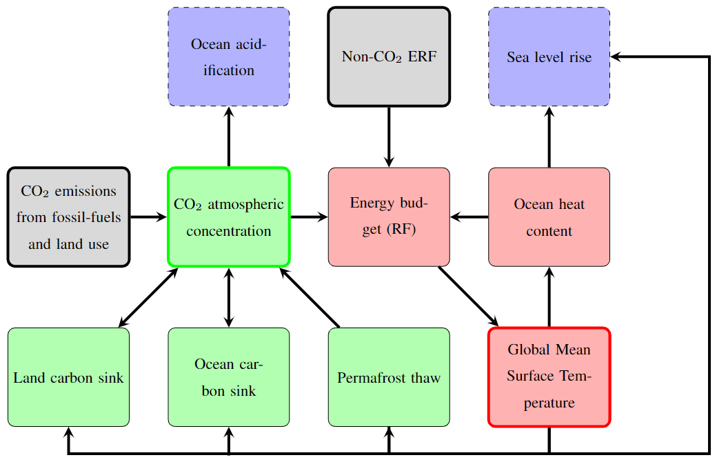
Figure 1 Pathfinder in a nutshell. Green blocks represent the carbon cycle, and red blocks represent the climate response. Blue blocks with dotted arrows are impacts that can be derived with the model. Grey blocks are variables that are directly related to anthropogenic activity. Possible inputs of the model are distinguishable through the bold contours of the blocks. In this scheme, arrows correspond to a forward mode where inputs would be $E_{{\mathrm{CO}}_{\mathrm{2}}}$ and R_x.

The following presents all equations of the models. Variables are noted using Roman letters and compiled in Tables B1 and B2. With a few exceptions, parameters are noted using Greek letters and are summarized in Tables B3 and B4. The model has 21 state variables that follow first-order differential equations in time. The time variable is denoted as t and kept implicit unless required.

2.1 Climate

The GMST change (T) induced by effective radiative forcing (ERF; R) is represented using a widely used two-box energy balance model with deep-ocean heat uptake efficacy (Geoffroy et al., 2013a; Armour, 2017). The first box represents the Earth surface's temperature (including atmosphere, land, and surface ocean), and the other one is the deep ocean's temperature (T_d). Their time-differential equations are

$$\begin{array}{}\text{(1)}& {\mathrm{\Theta }}_{\mathrm{s}}{\displaystyle \frac{\mathrm{d}T}{\mathrm{d}t}}=R-{\displaystyle \frac{\mathit{\varphi }\ln \left(\mathrm{2}\right)}{T_{\mathrm{2}\times }}}T-{\mathit{ϵ}}_{\mathrm{heat}}\mathit{\theta }(T-T_{\mathrm{d}}),\end{array}$$

and

$$\begin{array}{}\text{(2)}& {\mathrm{\Theta }}_{\mathrm{d}}{\displaystyle \frac{\mathrm{d}{T}_{\mathrm{d}}}{\mathrm{d}t}}=\mathit{\theta }(T-T_{\mathrm{d}}),\end{array}$$

where ϕ is the radiative parameter of CO₂, T_2× is the equilibrium climate sensitivity (ECS) at CO₂ doubling, Θ_s is the heat capacity of the surface, Θ_d is the heat capacity of the deep ocean, θ is the heat exchange coefficient, and ϵ_heat is the deep-ocean heat uptake efficacy.

The global ERF is simply the sum of the CO₂ contribution ($R_{{\mathrm{CO}}_{\mathrm{2}}}$) from its change in atmospheric concentration (C), expressed using the IPCC AR5 formula (Myhre et al., 2013), and that of non-CO₂ climate forcers (R_x):

$$\begin{array}{}\text{(3)}& R=R_{{\mathrm{CO}}_{\mathrm{2}}}+R_x,\end{array}$$

with

$$\begin{array}{}\text{(4)}& R_{{\mathrm{CO}}_{\mathrm{2}}}=\mathit{\varphi }\ln \left({\displaystyle \frac{C}{C_{\mathrm{pi}}}}\right),\end{array}$$

where C_pi is the preindustrial atmospheric CO₂ concentration.

The above energy balance model naturally provides the ocean heat content (OHC; U_ohc) as

$$\begin{array}{}\text{(5)}& U_{\mathrm{ohc}}={\mathit{\alpha }}_{\mathrm{ohc}}({\mathrm{\Theta }}_{\mathrm{s}}T+{\mathrm{\Theta }}_{\mathrm{d}}{T}_{\mathrm{d}}),\end{array}$$

and the ocean heat uptake (OHU) as

$$\begin{array}{}\text{(6)}& {\displaystyle \frac{\mathrm{d}{U}_{\mathrm{ohc}}}{\mathrm{d}t}}={\mathit{\alpha }}_{\mathrm{ohc}}\left({\mathrm{\Theta }}_{\mathrm{s}}{\displaystyle \frac{\mathrm{d}T}{\mathrm{d}t}}+{\mathrm{\Theta }}_{\mathrm{d}}{\displaystyle \frac{\mathrm{d}{T}_{\mathrm{d}}}{\mathrm{d}t}}\right),\end{array}$$

where α_ohc is the fraction of energy used to warm the ocean (i.e. excluding the energy needed to heat up the atmosphere and land and to melt ice).

2.2 Sea level rise

Global SLR has been implemented in Pathfinder as a variable of interest to model climate change impacts. In this version, it is firstly a proof of concept, modelled in a simple yet sensible manner. The total sea level rise (H_tot) is the sum of contributions from thermal expansion (H_thx), the Greenland ice sheet (GIS; H_gis), the Antarctic ice sheet (AIS; H_ais), and glaciers (H_gla):

$$\begin{array}{}\text{(7)}& H_{\mathrm{tot}}=H_{\mathrm{thx}}+H_{\mathrm{gis}}+H_{\mathrm{ais}}+H_{\mathrm{gla}}.\end{array}$$

The thermal expansion contribution scales linearly with the OHC (Goodwin et al., 2017; Fox-Kemper et al., 2021):

$$\begin{array}{}\text{(8)}& H_{\mathrm{thx}}={\mathrm{\Lambda }}_{\mathrm{thx}}{U}_{\mathrm{ohc}},\end{array}$$

where Λ_thx is the scaling factor of the thermosteric contribution to SLR. Note, however, that the thermal capacity of the climate module does not match that of the real-world ocean (Geoffroy et al., 2013b), and so this equation cannot describe equilibrium SLR over millennial timescales.

To model contributions from ice sheets and glaciers, we followed the general approach of Mengel et al. (2016). The SLR caused by GIS follows a first-order differential equation with its specific timescale, and the equilibrium SLR from GIS is assumed to be a cubic function of GMST:

$$\begin{array}{}\text{(9)}& {\displaystyle \frac{\mathrm{d}{H}_{\mathrm{gis}}}{\mathrm{d}t}}={\mathit{\lambda }}_{\mathrm{gis}}+{\displaystyle \frac{\mathrm{1}}{{\mathit{\tau }}_{\mathrm{gis}}}}\left({\mathrm{\Lambda }}_{\mathrm{gis}\mathrm{1}}T+{\mathrm{\Lambda }}_{\mathrm{gis}\mathrm{3}}{T}^{\mathrm{3}}-H_{\mathrm{gis}}\right),\end{array}$$

where λ_gis is an offset parameter introduced because GIS was not in a steady state at the end of the preindustrial era, Λ_gis1 is the linear term of equilibrium of GIS SLR, Λ_gis3 is the cubic term of equilibrium of GIS SLR, and τ_gis is the timescale of the GIS contribution. The motivation for replacing the quadratic term of Mengel et al. (2016) with a cubic one is the oddness of the cubic function that leads to negative (and not positive) SLR for negative T (which happens during the earlier years of the calibration run).

The contribution from glaciers is also a first-order differential equation with an equilibrium inspired by Mengel et al. (2016). We expanded it with a cubic term to account for the fact that we aggregate all glaciers together and allow more skewness in the curve describing the equilibrium SLR as a function of T. In addition, we added an exponential sensitivity to speed up the convergence to equilibrium under a warmer climate:

$$\begin{array}{}\text{(10)}& \begin{array}{rl}{\displaystyle \frac{\mathrm{d}{H}_{\mathrm{gla}}}{\mathrm{d}t}}& ={\mathit{\lambda }}_{\mathrm{gla}}+{\displaystyle \frac{\exp \left({\mathit{\gamma }}_{\mathrm{gla}}T\right)}{{\mathit{\tau }}_{\mathrm{gla}}}}\\ & \left({\mathrm{\Lambda }}_{\mathrm{gla}}\left(\mathrm{1}-\exp \left(-{\mathrm{\Gamma }}_{\mathrm{gla}\mathrm{1}}T-{\mathrm{\Gamma }}_{\mathrm{gla}\mathrm{3}}{T}^{\mathrm{3}}\right)\right)-H_{\mathrm{gla}}\right),\end{array}\end{array}$$

where λ_gla is an offset parameter accounting for the lack of initial steady state, Λ_gla is the SLR potential if all glaciers melted, Γ_gla1 is the linear sensitivity of glaciers' equilibrium to climate change, Γ_gla3 is the cubic sensitivity of glaciers' equilibrium to climate change, τ_gla is the timescale of the glaciers contribution, and γ_gla is the sensitivity of glaciers' timescale to climate change.

Following Mengel et al. (2016), the contribution from AIS is further divided into two terms, one for surface mass balance (SMB; H_ais,smb) and one for solid ice discharge (SID; H_ais,sid), so that $H_{\mathrm{ais}}=H_{\mathrm{ais},\mathrm{smb}}+H_{\mathrm{ais},\mathrm{sid}}$. It is expected that precipitation will increase over Antarctica under higher GMST, leading to an increase in SMB and to a negative sea level rise contribution modelled as

$$\begin{array}{}\text{(11)}& {\displaystyle \frac{\mathrm{d}{H}_{\mathrm{ais},\mathrm{smb}}}{\mathrm{d}t}}=-{\mathrm{\Lambda }}_{\mathrm{ais},\mathrm{smb}}T,\end{array}$$

where Λ_ais,smb is the AIS SMB sensitivity to climate change (expressed in sea level equivalent). At the same time, increasing surface ocean temperatures will cause more SID through basal melting, which we model using a first-order differential equation assumed to be independent of the SMB effect, and with a term that speeds up the effect the more SID happened:

$$\begin{array}{}\text{(12)}& {\displaystyle \frac{\mathrm{d}{H}_{\mathrm{ais},\mathrm{sid}}}{\mathrm{d}t}}={\mathit{\lambda }}_{\mathrm{ais}}+{\displaystyle \frac{\mathrm{1}+{\mathit{\alpha }}_{\mathrm{ais}}{H}_{\mathrm{ais},\mathrm{sid}}}{{\mathit{\tau }}_{\mathrm{ais}}}}\left({\mathrm{\Lambda }}_{\mathrm{ais}}T-H_{\mathrm{ais},\mathrm{sid}}\right),\end{array}$$

where λ_ais is an offset parameter accounting for the lack of initial steady state, Λ_ais is the SLR equilibrium of AIS SID, τ_ais is the timescale of the AIS SID contribution, and α_ais is the sensitivity of the timescale to past SID. In the model's code, however, we directly solve for the total AIS contribution as

$$\begin{array}{}\text{(13)}& \begin{array}{rl}{\displaystyle \frac{\mathrm{d}{H}_{\mathrm{ais}}}{\mathrm{d}t}}& =-{\mathrm{\Lambda }}_{\mathrm{ais},\mathrm{smb}}T+{\mathit{\lambda }}_{\mathrm{ais}}+{\displaystyle \frac{\mathrm{1}+{\mathit{\alpha }}_{\mathrm{ais}}(H_{\mathrm{ais}}-H_{\mathrm{ais},\mathrm{smb}})}{{\mathit{\tau }}_{\mathrm{ais}}}}\\ & \left({\mathrm{\Lambda }}_{\mathrm{ais}}T-(H_{\mathrm{ais}}-H_{\mathrm{ais},\mathrm{smb}})\right).\end{array}\end{array}$$

2.3 Ocean carbon

To calculate the ocean carbon sink, we use the classic mixed-layer impulse response function model from Joos et al. (1996), updated to the equivalent box model formulation of Strassmann and Joos (2018) and extended in places to introduce parameter adjustments for calibration. In the model, the mixed layer is split into five boxes (subscript j), as represented in Fig. 2, so that the total carbon in the mixed-layer pool (C_o) is

$$\begin{array}{}\text{(14)}& C_{\mathrm{o}}=\sum _j{C}_{\mathrm{o},j}.\end{array}$$

This total carbon mass is converted into a molar concentration of dissolved inorganic carbon (DIC; c_dic) as follows:

$$\begin{array}{}\text{(15)}& c_{\mathrm{dic}}={\displaystyle \frac{{\mathit{\alpha }}_{\mathrm{dic}}}{{\mathit{\beta }}_{\mathrm{dic}}}}{C}_{\mathrm{o}},\end{array}$$

where α_dic is a fixed conversion factor and β_dic is a scaling factor for the conversion. The latter can be seen as a factor multiplying the mixed-layer depth: it is 1 if the depth is unchanged from the original Strassmann and Joos (2018) model.

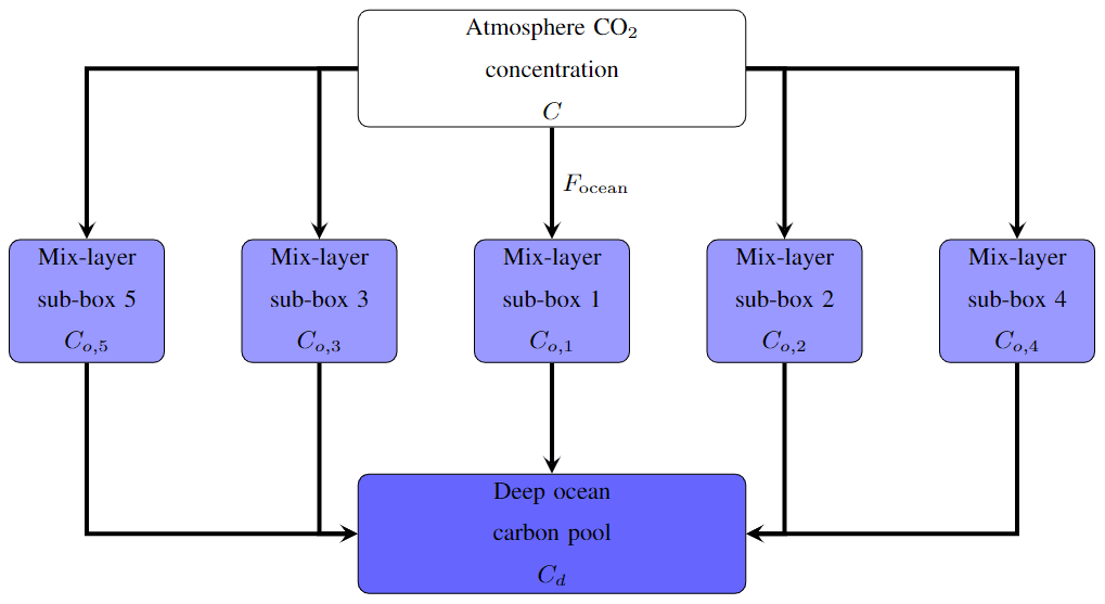
Figure 2 The ocean sink model in Pathfinder follows the structure of the mixed-layer pulse response function introduced by Joos et al. (1996). The mixed layer is represented through five sub-pools that each have a different timescale for transport to the deep-ocean carbon pool.

The non-linear carbonate chemistry in the mixed layer is emulated in two steps. First, the model's original polynomial function is used to determine the partial pressure of CO₂ affected by changes in DIC only (p_dic):

$$\begin{array}{}\text{(16)}& {\displaystyle }\begin{array}{rl}{p}_{\mathrm{dic}}=& (\mathrm{1.5568}-\mathrm{0.013993}{T}_{\mathrm{o}})c_{\mathrm{dic}}\\ +& (\mathrm{7.4706}-\mathrm{0.20207}{T}_{\mathrm{o}}){\mathrm{10}}^{-\mathrm{3}}{c_{\mathrm{dic}}}^{\mathrm{2}}\\ -& (\mathrm{1.2748}-\mathrm{0.12015}{T}_{\mathrm{o}}){\mathrm{10}}^{-\mathrm{5}}{c_{\mathrm{dic}}}^{\mathrm{3}}\\ +& (\mathrm{2.4491}-\mathrm{0.12639}{T}_{\mathrm{o}}){\mathrm{10}}^{-\mathrm{7}}{c_{\mathrm{dic}}}^{\mathrm{4}}\\ -& (\mathrm{1.5768}-\mathrm{0.15326}{T}_{\mathrm{o}}){\mathrm{10}}^{-\mathrm{10}}{c_{\mathrm{dic}}}^{\mathrm{5}},\end{array}\end{array}$$

where T_o is the preindustrial surface ocean temperature. Second, the actual partial pressure of CO₂ ($p_{{\mathrm{CO}}_{\mathrm{2}}}$) is calculated using an exponential climate sensitivity (Takahashi et al., 1993; Joos et al., 2001):

$$\begin{array}{}\text{(17)}& p_{{\mathrm{CO}}_{\mathrm{2}}}=(p_{\mathrm{dic}}+C_{\mathrm{pi}})\exp \left({\mathit{\gamma }}_{\mathrm{dic}}T\right),\end{array}$$

where γ_dic is the sensitivity of $p_{{\mathrm{CO}}_{\mathrm{2}}}$ to climate change.

The flux of carbon between the atmosphere and the ocean (F_ocean, defined positively if it is a carbon sink) is caused by the difference in partial pressure of CO₂ in the atmosphere and at the oceanic surface, following an exchange rate that varies linearly with GMST, that is here used as a proxy for wind changes:

$$\begin{array}{}\text{(18)}& F_{\mathrm{ocean}}={\mathit{\nu }}_{\mathrm{gx}}(\mathrm{1}+{\mathit{\gamma }}_{\mathrm{gx}}T)(C-p_{{\mathrm{CO}}_{\mathrm{2}}}),\end{array}$$

where ν_gx is the preindustrial gas exchange rate and γ_gx is its sensitivity to climate change.

This flux of carbon entering the ocean is split between the mixed-layer carbon sub-pools, and this added carbon is subsequently transported towards the deep ocean at a rate specific to each sub-pool. This leads to the following differential equations:

$$\begin{array}{}\text{(19)}& {\displaystyle \frac{\mathrm{d}{C}_{\mathrm{o},j}}{\mathrm{d}t}}=-{\displaystyle \frac{C_{\mathrm{o},j}}{{\mathit{\kappa }}_{{\mathit{\tau }}_{\mathrm{o}}}{\mathit{\tau }}_{\mathrm{o},j}}}+{\mathit{\alpha }}_{\mathrm{o},j}{F}_{\mathrm{ocean}},\forall j,\end{array}$$

where α_o,j are the sub-pools' splitting shares (with ${\sum }_j{\mathit{\alpha }}_{\mathrm{o},j}=\mathrm{1}$), τ_o,j are the sub-pools' timescales for transport to the deep ocean, and ${\mathit{\kappa }}_{{\mathit{\tau }}_{\mathrm{o}}}$ is a scaling factor applied to all sub-pools. Finally, the deep-ocean carbon pool (C_d) is obtained through mass balance:

$$\begin{array}{}\text{(20)}& {\displaystyle \frac{\mathrm{d}{C}_{\mathrm{d}}}{\mathrm{d}t}}=\sum _j{\displaystyle \frac{C_{\mathrm{o},j}}{{\mathit{\kappa }}_{{\mathit{\tau }}_{\mathrm{o}}}{\mathit{\tau }}_{\mathrm{o},j}}}.\end{array}$$

2.4 Ocean acidification

While in the real world, ocean acidification is directly related to the carbonate chemistry and the ocean uptake of anthropogenic carbon, we do not have a simple formulation at our disposal that could link it to our ocean carbon cycle module. We therefore use a readily available emulation of the surface ocean acidification (pH) that links it directly to the atmospheric concentration of CO₂ (Bernie et al., 2010) with the following polynomial approximation:

$$\begin{array}{}\text{(21)}& \begin{array}{rl}\mathrm{pH}& ={\mathit{\kappa }}_{\mathrm{pH}}\left(\mathrm{8.5541}-\mathrm{0.00173}C+\mathrm{1.3264}{\mathrm{10}}^{-\mathrm{6}}{C}^{\mathrm{2}}\right.\\ & \left.-\mathrm{4.4943}{\mathrm{10}}^{-\mathrm{10}}{C}^{\mathrm{3}}\right),\end{array}\end{array}$$

where κ_pH is a scaling factor (that defaults to 1). We note that this approach is reasonable for the surface ocean, as it quickly equilibrates with the atmosphere (but it would not work for the deep ocean).

2.5 Land carbon

The land carbon module of Pathfinder is a simplified version of the one in OSCAR (Gasser et al., 2017, 2020). It is shrunk down to four global carbon pools: vegetation, litter, and active and passive soil (see Fig. 3). All terrestrial biomes are lumped together, and there is therefore no accounting for the impact of land use change on the land carbon cycle in this version of Pathfinder. This is an extreme assumption – although very common in SCMs – motivated by simplicity, and it implies that CO₂ emissions from fossil fuel burning and land use change are assumed to behave in the exact same way, in spite of their not doing so in reality (Gitz and Ciais, 2003; Gasser and Ciais, 2013).

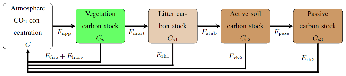
Figure 3 The land sink model in Pathfinder is derived from OSCAR (Gasser et al., 2017) and represents the biosphere as a set of four carbon pools: vegetation, litter, and active and passive soil. These pools exchange carbon through fluxes whose direction is given by the arrows.

The vegetation carbon pool (C_v) results from the balance between net primary productivity (NPP; F_npp), emission from wildfires (E_fire), emission from harvest and grazing (E_harv), and loss of carbon from biomass mortality (F_mort):

$$\begin{array}{}\text{(22)}& {\displaystyle \frac{\mathrm{d}{C}_{\mathrm{v}}}{\mathrm{d}t}}=F_{\mathrm{npp}}-E_{\mathrm{fire}}-E_{\mathrm{harv}}-F_{\mathrm{mort}}.\end{array}$$

NPP is expressed as its own preindustrial value multiplied by a function of CO₂ and of GMST (r_npp). This function thus embeds the so-called CO₂ fertilization effect, whereby NPP increases with atmospheric CO₂, described using a generalized logarithmic functional form:

$$\begin{array}{}\text{(23)}& F_{\mathrm{npp}}=F_{\mathrm{npp}\mathrm{0}}{r}_{\mathrm{npp}},\end{array}$$

with

$$\begin{array}{}\text{(24)}& r_{\mathrm{npp}}=\left(\mathrm{1}+{\displaystyle \frac{{\mathit{\beta }}_{\mathrm{npp}}}{{\mathit{\alpha }}_{\mathrm{npp}}}}\left(\mathrm{1}-{\left({\displaystyle \frac{C}{C_{\mathrm{pi}}}}\right)}^{-{\mathit{\alpha }}_{\mathrm{npp}}}\right)\right)(\mathrm{1}+{\mathit{\gamma }}_{\mathrm{npp}}T),\end{array}$$

where F_npp0 is the preindustrial NPP, β_npp is the CO₂ fertilization sensitivity, α_npp is the CO₂ fertilization shape parameter for saturation, and γ_npp is the sensitivity of NPP to climate change (that can be positive or negative). The generalized logarithmic functional form implies that $r_{\mathrm{npp}}\to (\mathrm{1}+{\mathit{\beta }}_{\mathrm{npp}}\ln (C/C_{\mathrm{pi}}\left)\right)(\mathrm{1}+{\mathit{\gamma }}_{\mathrm{npp}}T)$ as ${\mathit{\alpha }}_{\mathrm{npp}}\to {\mathrm{0}}^{+}$.

Harvesting and mortality fluxes are taken proportional to the carbon pool itself even though in reality the mortality fluxes are climate dependent. For simplicity we assume a constant mortality following the equations in OSCAR (Gasser et al., 2017):

$$\begin{array}{}\text{(25)}& E_{\mathrm{harv}}={\mathit{\nu }}_{\mathrm{harv}}{C}_{\mathrm{v}},\end{array}$$

and

$$\begin{array}{}\text{(26)}& F_{\mathrm{mort}}={\mathit{\nu }}_{\mathrm{mort}}{C}_{\mathrm{v}},\end{array}$$

where ν_harv is the harvesting or grazing rate and ν_mort is the mortality rate.

Wildfires emissions are also assumed to be proportional to the vegetation carbon pool, but with an additional linear dependency of the emission rate on CO₂ (as a proxy of changes in leaf area index and evapotranspiration) and GMST (r_fire):

$$\begin{array}{}\text{(27)}& E_{\mathrm{fire}}={\mathit{\nu }}_{\mathrm{fire}}{r}_{\mathrm{fire}}{C}_{\mathrm{v}},\end{array}$$

with

$$\begin{array}{}\text{(28)}& r_{\mathrm{fire}}=\left(\mathrm{1}+{\mathit{\beta }}_{\mathrm{fire}}\left({\displaystyle \frac{C}{C_{\mathrm{pi}}}}-\mathrm{1}\right)\right)(\mathrm{1}+{\mathit{\gamma }}_{\mathrm{fire}}T),\end{array}$$

where ν_fire is the wildfire rate, β_fire is the sensitivity of wildfires to CO₂, and γ_fire is their sensitivity to climate change.

Soil carbon is divided into three pools. The litter carbon pool (C_s1) receives the mortality flux as sole input, it emits part of its carbon through heterotrophic respiration (E_rh1), and it transfers another part to the next pool through stabilization (F_stab):

$$\begin{array}{}\text{(29)}& {\displaystyle \frac{\mathrm{d}{C}_{\mathrm{s}\mathrm{1}}}{\mathrm{d}t}}=F_{\mathrm{mort}}-F_{\mathrm{stab}}-E_{\mathrm{rh}\mathrm{1}}.\end{array}$$

Similarly, the active soil carbon pool (C_s2) receives the stabilization flux, is respired (E_rh2), and transfers carbon to the last pool through passivization (F_pass):

$$\begin{array}{}\text{(30)}& {\displaystyle \frac{\mathrm{d}{C}_{\mathrm{s}\mathrm{2}}}{\mathrm{d}t}}=F_{\mathrm{stab}}-F_{\mathrm{pass}}-E_{\mathrm{rh}\mathrm{2}}.\end{array}$$

The passive carbon pool (C_s3) receives this final input flux and is respired (E_rh3):

$$\begin{array}{}\text{(31)}& {\displaystyle \frac{\mathrm{d}{C}_{\mathrm{s}\mathrm{3}}}{\mathrm{d}t}}=F_{\mathrm{pass}}-E_{\mathrm{rh}\mathrm{3}}.\end{array}$$

Although information pertaining to this fourth pool is not commonly provided by ESMs, it was introduced in Pathfinder to adjust the complex models' turnover time of soil carbon to better match isotopic data (He et al., 2016). For completeness, we note that the total heterotrophic respiration is $E_{\mathrm{rh}}=E_{\mathrm{rh}\mathrm{1}}+E_{\mathrm{rh}\mathrm{2}}+E_{\mathrm{rh}\mathrm{3}}$, and the total soil carbon pool is $C_{\mathrm{s}}=C_{\mathrm{s}\mathrm{1}}+C_{\mathrm{s}\mathrm{2}}+C_{\mathrm{s}\mathrm{3}}$.

All soil-originating fluxes are taken proportional to their pool of origin and multiplied by a function (r_rh) explained hereafter. For the litter pool, this gives

$$\begin{array}{}\text{(32)}& E_{\mathrm{rh}\mathrm{1}}={\mathit{\nu }}_{\mathrm{rh}\mathrm{1}}{r}_{\mathrm{rh}}{C}_{\mathrm{s}\mathrm{1}},\end{array}$$

and

$$\begin{array}{}\text{(33)}& F_{\mathrm{stab}}={\mathit{\nu }}_{\mathrm{stab}}{r}_{\mathrm{rh}}{C}_{\mathrm{s}\mathrm{1}},\end{array}$$

where ν_rh1 is the litter respiration rate and ν_stab is the stabilization rate. For the active soil pool, we have

$$\begin{array}{}\text{(34)}& E_{\mathrm{rh}\mathrm{2}}={\displaystyle \frac{{\mathit{\nu }}_{\mathrm{rh}\mathrm{23}}-{\mathit{\nu }}_{\mathrm{rh}\mathrm{3}}{\mathit{\alpha }}_{\mathrm{pass}}}{\mathrm{1}-{\mathit{\alpha }}_{\mathrm{pass}}}}{r}_{\mathrm{rh}}{C}_{\mathrm{s}\mathrm{2}},\end{array}$$

and

$$\begin{array}{}\text{(35)}& F_{\mathrm{pass}}={\mathit{\nu }}_{\mathrm{rh}\mathrm{3}}{\displaystyle \frac{{\mathit{\alpha }}_{\mathrm{pass}}}{\mathrm{1}-{\mathit{\alpha }}_{\mathrm{pass}}}}{r}_{\mathrm{rh}}{C}_{\mathrm{s}\mathrm{2}},\end{array}$$

and for the passive soil pool:

$$\begin{array}{}\text{(36)}& E_{\mathrm{rh}\mathrm{3}}={\mathit{\nu }}_{\mathrm{rh}\mathrm{3}}{r}_{\mathrm{rh}}{C}_{\mathrm{s}\mathrm{3}},\end{array}$$

where ν_rh23 is the soil respiration rate (averaged over active and passive pools), ν_rh3 is the passive soil respiration rate, and α_pass is the fraction of passive carbon (over active plus passive soil carbon). This slightly convoluted formulation is motivated by the lack of information regarding the active/passive split in ESMs, which we alleviate using additional data during calibration.

In addition, the function r_rh, describing the dependency of respiration (and related fluxes) on temperature and on the availability of fresh organic matter to be decomposed, is defined as follows:

$$\begin{array}{}\text{(37)}& \begin{array}{rl}& r_{\mathrm{rh}}=\\ & \underset{\left(\mathrm{1}+{\mathit{\beta }}_{\mathrm{rh}}\left(\frac{C_{\mathrm{s}\mathrm{1}}}{C_{\mathrm{s}}}\frac{C_{\mathrm{s}}\left(t_{\mathrm{0}}\right)}{C_{\mathrm{s}\mathrm{1}}\left(t_{\mathrm{0}}\right)}-\mathrm{1}\right)\right)}{\underbrace{\left(\mathrm{1}+{\mathit{\beta }}_{\mathrm{rh}}\left({\displaystyle \frac{C_{\mathrm{s}\mathrm{1}}}{C_{\mathrm{s}\mathrm{1}}+C_{\mathrm{s}\mathrm{2}}+C_{\mathrm{s}\mathrm{3}}}}\left(\mathrm{1}+{\displaystyle \frac{{\mathit{\nu }}_{\mathrm{stab}}}{{\mathit{\nu }}_{\mathrm{rh}\mathrm{23}}}}\right)-\mathrm{1}\right)\right)}}\exp \left({\mathit{\gamma }}_{\mathrm{rh}}T\right),\end{array}\end{array}$$

where β_rh is the sensitivity of the respiration to fresh organic matter availability (expressed here as the relative change in the $C_{\mathrm{s}\mathrm{1}}/C_{\mathrm{s}}$ ratio with regard to preindustrial times), and γ_rh is its sensitivity to climate change (equivalent to a “Q₁₀” formulation with Q₁₀=exp (10 γ_rh)).

Finally, the net carbon flux from the atmosphere to the land (F_land, defined positively if it is a carbon sink) is obtained as the net budget of all pools combined:

$$\begin{array}{}\text{(38)}& F_{\mathrm{land}}=F_{\mathrm{npp}}-E_{\mathrm{fire}}-E_{\mathrm{harv}}-E_{\mathrm{rh}},\end{array}$$

and this system of equations leads to the following preindustrial steady state:

$$\begin{array}{}\text{(39)}& \left\{\begin{array}{l}{C}_{\mathrm{v}}\left(t_{\mathrm{0}}\right)=\frac{F_{\mathrm{npp}\mathrm{0}}}{{\mathit{\nu }}_{\mathrm{fire}}+{\mathit{\nu }}_{\mathrm{harv}}+{\mathit{\nu }}_{\mathrm{mort}}}\\ C_{\mathrm{s}\mathrm{1}}\left(t_{\mathrm{0}}\right)=C_{\mathrm{v}}\left(t_{\mathrm{0}}\right)\frac{{\mathit{\nu }}_{\mathrm{mort}}}{{\mathit{\nu }}_{\mathrm{rh}\mathrm{1}}+{\mathit{\nu }}_{\mathrm{stab}}}\\ C_{\mathrm{s}\mathrm{2}}\left(t_{\mathrm{0}}\right)=C_{\mathrm{s}\mathrm{1}}\left(t_{\mathrm{0}}\right)\frac{{\mathit{\nu }}_{\mathrm{stab}}}{{\mathit{\nu }}_{\mathrm{rh}\mathrm{23}}}(\mathrm{1}-{\mathit{\alpha }}_{\mathrm{pass}})\\ C_{\mathrm{s}\mathrm{3}}\left(t_{\mathrm{0}}\right)=C_{\mathrm{s}\mathrm{1}}\left(t_{\mathrm{0}}\right)\frac{{\mathit{\nu }}_{\mathrm{stab}}}{{\mathit{\nu }}_{\mathrm{rh}\mathrm{23}}}{\mathit{\alpha }}_{\mathrm{pass}}.\end{array}\right.\end{array}$$

2.6 Permafrost carbon

As the land carbon cycle described in the previous section does not account for permafrost carbon, we implemented this feedback using the emulator developed by Gasser et al. (2018) but aggregated into a unique global region. Figure 4 gives a representation of the permafrost module as described in the following. The emulation starts with a theoretical thawed fraction ($\overline{a}$) that represents the fraction of thawed carbon under steady-state for a certain level of local warming. It is formulated with a sigmoid function (that equals 0 at preindustrial and 1 under very high GMST):

$$\begin{array}{}\text{(40)}& \begin{array}{rl}& \overline{a}=\\ & -a_{\min }+{\displaystyle \frac{(\mathrm{1}+a_{\min })}{{\left(\mathrm{1}+\left({\left(\mathrm{1}+\frac{\mathrm{1}}{a_{\min }}\right)}^{{\mathit{\kappa }}_a}-\mathrm{1}\right)\exp (-{\mathit{\gamma }}_a{\mathit{\kappa }}_a{\mathit{\alpha }}_{\mathrm{lst}}T)\right)}^{\frac{\mathrm{1}}{{\mathit{\kappa }}_a}}}},\end{array}\end{array}$$

where −a_min is the minimum thawed fraction (corresponding to 100 % frozen soil carbon), κ_a is a shape parameter determining the asymmetry of the function, γ_a is the sensitivity of the theoretical thawed fraction to local climate change, and α_lst is the proportionality factor between local and global climate change.

Figure 4 The permafrost carbon model in Pathfinder is taken from Gasser et al. (2018). The frozen pool dynamic lags behind a theoretical value that is determined by the temperature anomaly. Thawed carbon is then split between three pools that are emitted to the atmosphere at different rates.

The actual thawed fraction (a) then moves towards its theoretical value at a speed that depends on whether it is thawing (i.e. $a<\overline{a}$) or freezing (i.e. $a>\overline{a}$). This is written as a non-linear differential equation:

$$\begin{array}{}\text{(41)}& \begin{array}{rl}{\displaystyle \frac{\mathrm{d}a}{\mathrm{d}t}}& =\mathrm{0.5}({\mathit{\nu }}_{\mathrm{thaw}}+{\mathit{\nu }}_{\mathrm{froz}})(\overline{a}-a)\\ & +\mathrm{0.5}\left|\right({\mathit{\nu }}_{\mathrm{thaw}}-{\mathit{\nu }}_{\mathrm{froz}}\left)\right(\overline{a}-a\left)\right|,\end{array}\end{array}$$

where ν_thaw is the rate of thawing and ν_froz is the rate of freezing. Because ν_thaw>ν_froz, the absolute value in the equation leads to the right-hand side being ${\mathit{\nu }}_{\mathrm{thaw}}(\overline{a}-a)$ if $a<\overline{a}$, or ${\mathit{\nu }}_{\mathrm{froz}}(\overline{a}-a)$ if $a>\overline{a}$. The change in the pool of frozen carbon (C_fr) naturally follows:

$$\begin{array}{}\text{(42)}& {\displaystyle \frac{\mathrm{d}{C}_{\mathrm{fr}}}{\mathrm{d}t}}=-{\displaystyle \frac{\mathrm{d}a}{\mathrm{d}t}}{C}_{\mathrm{fr}\mathrm{0}},\end{array}$$

where C_fr0 is the amount of frozen carbon at preindustrial times.

Thawed carbon is not directly emitted to the atmosphere: it is split into three thawed carbon sub-pools (C_th,j) that have their own decay time but are all affected by an additional function (r_rt). This leads to the following budget equations:

$$\begin{array}{}\text{(43)}& {\displaystyle \frac{\mathrm{d}{C}_{\mathrm{th},j}}{\mathrm{d}t}}=-{\mathit{\alpha }}_{\mathrm{th},j}{\displaystyle \frac{\mathrm{d}{C}_{\mathrm{fr}}}{\mathrm{d}t}}-{\displaystyle \frac{C_{\mathrm{th},j}}{{\mathit{\kappa }}_{{\mathit{\tau }}_{\mathrm{th}}}{\mathit{\tau }}_{\mathrm{th},j}}}{r}_{\mathrm{rt}},\forall j,\end{array}$$

where α_th,j is the sub-pools' splitting shares (with ${\sum }_j{\mathit{\alpha }}_{\mathrm{th},j}=\mathrm{1}$), τ_th,j is the sub-pools' decay times, and ${\mathit{\kappa }}_{{\mathit{\tau }}_{\mathrm{th}}}$ is a scaling factor applied to all sub-pools. The additional r_rt function describes the sensitivity of heterotrophic respiration to climate change in boreal regions using a Gaussian formula:

$$\begin{array}{}\text{(44)}& r_{\mathrm{rt}}=\exp \left({\mathit{\kappa }}_{\mathrm{rt}}{\mathit{\gamma }}_{\mathrm{rt}\mathrm{1}}{\mathit{\alpha }}_{\mathrm{lst}}T-{\mathit{\kappa }}_{\mathrm{rt}}{\mathit{\gamma }}_{\mathrm{rt}\mathrm{2}}({\mathit{\alpha }}_{\mathrm{lst}}T{)}^{\mathrm{2}}\right),\end{array}$$

where κ_rt is a factor scaling the sensitivity of thawed carbon against that of regular soil carbon, γ_rt1 is the sensitivity to local temperature change (i.e. a Q10), and γ_rt2 is the quadratic term in the latter sensitivity that represents a saturation effect. Noting that all the emitted carbon is assumed to be CO₂, the global emission from permafrost (E_pf) is thus

$$\begin{array}{}\text{(45)}& E_{\mathrm{pf}}=\sum _j{\displaystyle \frac{C_{\mathrm{th},j}}{{\mathit{\kappa }}_{{\mathit{\tau }}_{\mathrm{th}}}{\mathit{\tau }}_{\mathrm{th},j}}}{r}_{\mathrm{rt}}.\end{array}$$

2.7 Atmospheric CO₂

The change in atmospheric concentration of CO₂ is the budget of all carbon cycle fluxes to which we add the exogenous anthropogenic emissions ($E_{{\mathrm{CO}}_{\mathrm{2}}}$):

$$\begin{array}{}\text{(46)}& {\mathit{\alpha }}_{\mathrm{C}}{\displaystyle \frac{\mathrm{d}C}{\mathrm{d}t}}=E_{{\mathrm{CO}}_{\mathrm{2}}}+E_{\mathrm{pf}}-F_{\mathrm{land}}-F_{\mathrm{ocean}},\end{array}$$

where α_C is the conversion factor from volume fraction to mass for CO₂.

3 Bayesian calibration

3.1 Principle

Bayesian inference is a powerful tool for assimilating observational data into reduced-complexity models such as Pathfinder (Ricciuto et al., 2008). The approach consists in deducing probability distributions of parameters from a priori knowledge on those distributions and on distributions of observations of some of the model's variables, using Bayes' theorem (Bayes, 1763). Summarily, the Bayesian calibration updates the joint distribution of parameters to make it as compatible with the constraints as possible given their prior estimates, which increases the internal coherence of Pathfinder by excluding combination of parameters that are unlikely.

Such a Bayesian calibration is vulnerable to the possibility that the priors draw on the same information as the constraints. However, given that Pathfinder is a patchwork of emulators whose parameters are obtained independently from one another and following differing experimental setups, we expect that the coherence of information contained within the priors and the constraints is very low. Our choice of using only complex models as prior information and only observations and assessments as constraints also aims at limiting this vulnerability.

Concretely, the posterior probability 𝒫_post of a sample k from the joint parameters distribution ξ_k, conditional to a set of observations x, is proportional (symbol ∝) to its own prior probability 𝒫_pre and to the likelihood ℒ of the model simulating x given ξ_k:

$$\begin{array}{}\text{(47)}& {\mathcal{P}}_{\mathrm{post}}\left({\mathit{\xi }}_k\mathrm{|}\mathit{x}\right)\propto \mathcal{L}\left(\mathit{x}\mathrm{|}{\mathit{\xi }}_k\right){\mathcal{P}}_{\mathrm{pre}}\left({\mathit{\xi }}_k\right).\end{array}$$

Here, we assume all observations are independently and identically distributed following a normal distribution (with mean values μ_x, and standard deviations σ_x expressed in real physical units), which leads to the following likelihood:

$$\begin{array}{}\text{(48)}& \mathcal{L}\left(\mathit{x}\mathrm{|}{\mathit{\xi }}_k\right)=\prod _{i=\mathrm{1}}^{n_x}{\displaystyle \frac{\mathrm{1}}{{\mathit{\sigma }}_{x,i}\sqrt{\mathrm{2}\mathit{\pi }}}}\exp \left(-{\displaystyle \frac{\left({\mathcal{F}}_i\right({\mathit{\xi }}_k)-{\mathit{\mu }}_{x,i}{)}^{\mathrm{2}}}{\mathrm{2}{\mathit{\sigma }}_{x,i}^{\mathrm{2}}}}\right),\end{array}$$

where ℱ_i(ξ_k) is the model's output for the ith observable (out of n_x) with input parameters ξ_k.

3.2 Implementation

The Pathfinder model is a set of differential equations with a number of input parameters, of which n_ξ are calibrated through Bayesian inference, and an additional two input variables provided as time series (i.e. one value per time step required). While the two input time series can be any combination of two out of four variables (anthropogenic CO₂ emissions, non-CO₂ ERF, atmospheric CO₂ concentration, or GMST), for calibration we use the two most well-constrained variables that are direct physical observations of the global Earth system: atmospheric CO₂ and GMST. These input time series cover the historical period from 1751 to 2020. Therefore, the ξ_k vector is

$$\begin{array}{}\text{(49)}& {\mathit{\xi }}_k={\left\{\mathit{\{}{\mathit{\xi }}_j{\mathit{\}}}_{j=\mathrm{1}}^{n_{\mathit{\xi }}},\mathit{\{}C\left(t\right){\mathit{\}}}_{t=\mathrm{1751}}^{\mathrm{2021}},\mathit{\left\{}T\right(t){\mathit{\}}}_{t=\mathrm{1751}}^{\mathrm{2021}}\right\}}_k.\end{array}$$

However, to ease the computation by reducing the dimension of the system, we do not use annual time series of observations as inputs, but we assume that each input time series (for variable X being C or T) follows

$$\begin{array}{}\text{(50)}& X\left(t\right)=X_{\mathit{\mu }}\left(t\right)+{\stackrel{\mathrm{̃}}{\mathit{\sigma }}}_X{X}_{\mathit{\sigma }}\left(t\right)+{\mathit{ϵ}}_X\mathrm{AR}\mathrm{1}(t;{\mathit{\rho }}_X),\end{array}$$

where X_μ and X_σ are fixed exogenous annual time series (i.e. structural parameters), ${\stackrel{\mathrm{̃}}{\mathit{\sigma }}}_X$ is the relative standard deviation of the time series (without noise), ϵ_X is the noise intensity, and AR1 is an autoregressive process of order 1 and autocorrelation parameter ρ_X. This assumption leads to the final expression of the ξ_k vector:

$$\begin{array}{}\text{(51)}& {\mathit{\xi }}_k={\left\{\mathit{\{}{\mathit{\xi }}_j{\mathit{\}}}_{j=\mathrm{1}}^{n_{\mathit{\xi }}},{\stackrel{\mathrm{̃}}{\mathit{\sigma }}}_{\mathrm{C}},{\mathit{ϵ}}_{\mathrm{C}},{\mathit{\rho }}_{\mathrm{C}},{\stackrel{\mathrm{̃}}{\mathit{\sigma }}}_T,{\mathit{ϵ}}_T,{\mathit{\rho }}_T,\right\}}_k.\end{array}$$

During this Bayesian assimilation, the Pathfinder model is run solely over the historical period (from 1750 to 2021), as the constraints concern only preindustrial or historical years. For the computation, the time-differential system of Pathfinder is solved using an implicit–explicit numerical scheme (also called IMEX), with a time step of a quarter of a year. This solving scheme relies on writing the differential equations of all state variables X as

$$\begin{array}{}\text{(52)}& {\displaystyle \frac{\mathrm{d}X}{\mathrm{d}t}}=-\mathit{\nu }X+\mathcal{R},\end{array}$$

where ν is the constant speed of the linear part of the differential equation and ℛ is its non-linear part, discretizing these equations as

$$\begin{array}{}\text{(53)}& {\displaystyle \frac{X(t+\mathit{\delta }t)-X\left(t\right)}{\mathit{\delta }t}}=-\mathit{\nu }X(t+\mathit{\delta }t)+\mathcal{R}\left(t\right),\end{array}$$

where δt is the solving time step (which is $\frac{\mathrm{1}}{n_t}$ times the annual time step of the model's inputs and outputs, here n_t=4), and finally explicitly solving for all X(t+δt). We note this is also the default solving scheme for regular simulations with the model, although the value of n_t can be altered and alternative schemes are available.

The Bayesian procedure itself is implemented using the Python computer language and specifically the PyMC3 package (Salvatier et al., 2016). The solving of Eq. (47) and its normalization are done using the package's full-rank automatic differentiation variational inference (ADVI) algorithm (Kucukelbir et al., 2017), with 100 000 iterations (and default algorithm options). The choice of variational inference instead of Markov chain Monte Carlo is motivated by the significant size of our model (Blei et al., 2017) and the speed of ADVI. An additional strength of the full-rank version of the ADVI algorithm is its ability to generate correlated posterior distributions even if the prior ones are uncorrelated. Convergence of the algorithm was controlled through convergence of the ELBO metric (Kucukelbir et al., 2017). All results presented hereafter are obtained through drawing 2000 sets of parameters – which we call configurations – from the posterior or prior distributions.

3.3 Constraints

We use a set of 19 constraints related to all aspects of the model that correspond to the set of observations x in the Bayesian calibration. Many of the constraints are observations, but some are ranges assessed by expert panels such as the Global Carbon Project or the IPCC. They cover either a recent point in time or an assumed preindustrial equilibrium, and they are typically taken over a period of at least a few years to reduce the effect of natural variability.

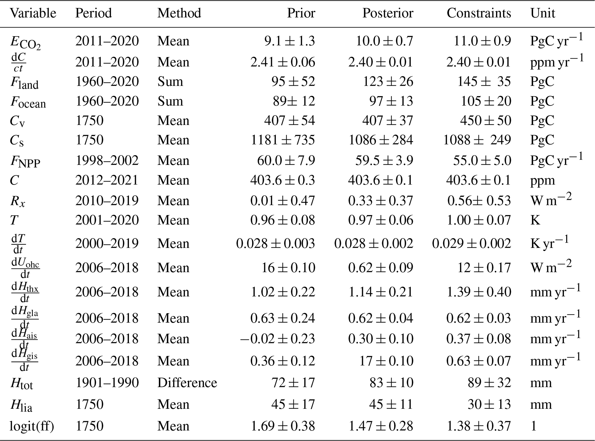
Table 1 summarizes these constraints, the periods over which they are considered, and their distributions. The following subsections provide further details on the constraints, and the constraint distributions are shown in Fig. 6.

Table 1 Constrained variables in Pathfinder, with values before and after calibration. Variables are noted under their text notation, and Tables B1 and B2 provide the corresponding notation in code. The uncertainty correspond to the 1σ uncertainty range.

3.3.1 Climate system

To constrain the temperature response, we use the same five data sets of observed GMST as in Sect. 3.4.8 to derive average and standard deviation of two constraints: the average GMST change and the average GMST yearly trend obtained through second-order accuracy gradient (Fornberg, 1988), both over the latest 20 years of data (2002–2021). Because these data sets are already used as input to the Bayesian setup, albeit in a different way, they do not provide much of a constraint and are used mostly to ensure that the ${\stackrel{\mathrm{̃}}{\mathit{\sigma }}}_T$ and ϵ_T parameters remain within sensible range.

To further constrain the climate system, we use the mean OHU assessed by the IPCC AR6 over 2006–2018 (Gulev et al., 2021, Table 2.7) and the non-CO₂ ERF (averaged over 2010-2019) also estimated for the AR6. The central value of the latter is taken from Dentener et al. (2021, Table AIII.3, and corresponding GitHub repository), and its uncertainty is constructed using data from Forster et al. (2021, Table 7.8) and assuming the ERF of all species are normally distributed and uncorrelated, but fully correlated in time for each separate species (which likely overestimates the uncertainty).

To better align with the IPCC AR6, we also constrain the ECS of our model (i.e. the T_2× parameters). To do so, because the distribution of ECS cannot be assumed to be normal, we follow the framework of Roe and Baker (2007), who define the climate feedback factor ff so that $T_{\mathrm{2}\times }=T_{\mathrm{2}\times }^{*}/(\mathrm{1}-\mathrm{ff})$, where $T_{\mathrm{2}\times }^{*}$ is the minimal ECS value (roughly corresponding to the Planck feedback). We assume this feedback factor follows a logit-normal distribution, which implies logit(ff) = $\ln (\mathrm{ff}/(\mathrm{1}-\mathrm{ff}\left)\right)$ = $\ln (T_{\mathrm{2}\times }/T_{\mathrm{2}\times }^{*}-\mathrm{1})$ follows a normal distribution. We therefore constrain logit(ff), using distribution parameters and a value of $T_{\mathrm{2}\times }^{*}$ calibrated to fit the probabilistic ranges of ECS provided by the AR6. This fit of the ECS distribution is illustrated in Fig. B9.

3.3.2 Carbon cycle

Similarly to what is done with GMST, we constrain the atmospheric CO₂ level over the latest 10 years of data (2012–2021) using the NOAA/ESRL data (Tans and Keeling, 2010). The rest of the global CO₂ budget is constrained using the 2021 Global Carbon Budget (GCB; Friedlingstein et al., 2022). We use the net atmospheric CO₂ growth and total anthropogenic emissions (fossil and land use) over the last 10 years and the ocean and land carbon sinks accumulated since the beginning of the instrumental measurement period (1960–2020). Note that our definition of the land carbon sink ignoring land use change is consistent with that of the GCB.

Given its number of parameters and their inconsistent sources, we further constrain the land carbon module by considering present-day (mean over 1998–2002) NPP (Ciais et al., 2013; Zhao et al., 2005) and preindustrial vegetation and soil carbon pools. These preindustrial pools are taken from the AR6 for the central value (Canadell et al., 2021, Fig. 5.12), but their relative uncertainty is taken from the AR5 (Ciais et al., 2013, Fig. 6.1) since it is lacking in the AR6. In addition, the soil carbon pool constraint is corrected downward by estimates of peatland carbon (Yu et al., 2010, Table 1), since it is an ecosystem missing in TRENDY models (and in ours) but not in the IPCC assessments.

3.3.3 Sea level rise

To constrain the separate SLR contributions from thermal expansion, GIS, AIS, and glaciers, we use the model-based SLR speed estimates over the recent past (averaged over 2006–2018) reported in the AR6 (Fox-Kemper et al., 2021, Table 9.5). To constrain the total contribution, we also use the historical (1901–1990) sea level rise inferred from tide gauges from the same source, although the value is corrected upward for the missed impact of uncharted glaciers (Parkes and Marzeion, 2018).

Contrarily to all other modules, the SLR module is not assumed to start at steady state in 1750, which is represented through the λ_ice ($\mathrm{ice}\in [\mathrm{gla},\mathrm{gis},\mathrm{ais}]$) parameters. We assume this is entirely due to the so-called Little Ice Age (LIA) relaxation, which we assume can be simply modelled in Pathfinder through exponential decay of our three ice-related contributions since t₀=1750. This gives a net LIA contribution of $H_{\mathrm{lia}}={\sum }_{\mathrm{ice}}{\mathit{\lambda }}_{\mathrm{ice}}{\mathit{\tau }}_{\mathrm{ice}}\exp \left(-\frac{t-t_{\mathrm{0}}}{{\mathit{\tau }}_{\mathrm{ice}}}\right)$. We constrain this diagnostic variable using the global SLR reported by Slangen et al. (2016) over 1900–2005 for their control experiment.

3.4 Parameters (prior distributions)

Out of the model's 77 parameters, 33 are assumed to be fixed (i.e. they are structural parameters), and the remaining n_ξ=44 parameters are estimated through Bayesian inference. Prior distributions of the ξ_j parameters are assumed log-normal if the physical parameter must be defined positive, logit-normal if it must be between 0 and 1, and normal otherwise. To avoid extreme parameter values that could make the model diverge during calibration, the posterior distributions are bound to ${\mathit{\mu }}_{\mathit{\xi },j}\pm \mathrm{5}{\mathit{\sigma }}_{\mathit{\xi },j}$, where μ_ξ,j and σ_ξ,j are the mean and standard deviation of the jth parameter's prior distribution. These two values are taken from the literature, deduced from multi-model ensembles, or in a few instances arbitrarily set, as described in the following subsections. Note that when parameters are deduced from multi-model ensembles, there are effectively two rounds of calibration: first, a calibration on individual models using ordinary least-squares regressions to obtain prior distributions and, second, the Bayesian calibration itself that leads to the posterior distributions. In addition, the prior distributions of ${\stackrel{\mathrm{̃}}{\mathit{\sigma }}}_X$, ϵ_X and ρ_X are assumed normal, half-normal, and uniform, respectively. All prior distributions are assumed independent, meaning that the prior joint distribution ξ does not exhibit any covariance.

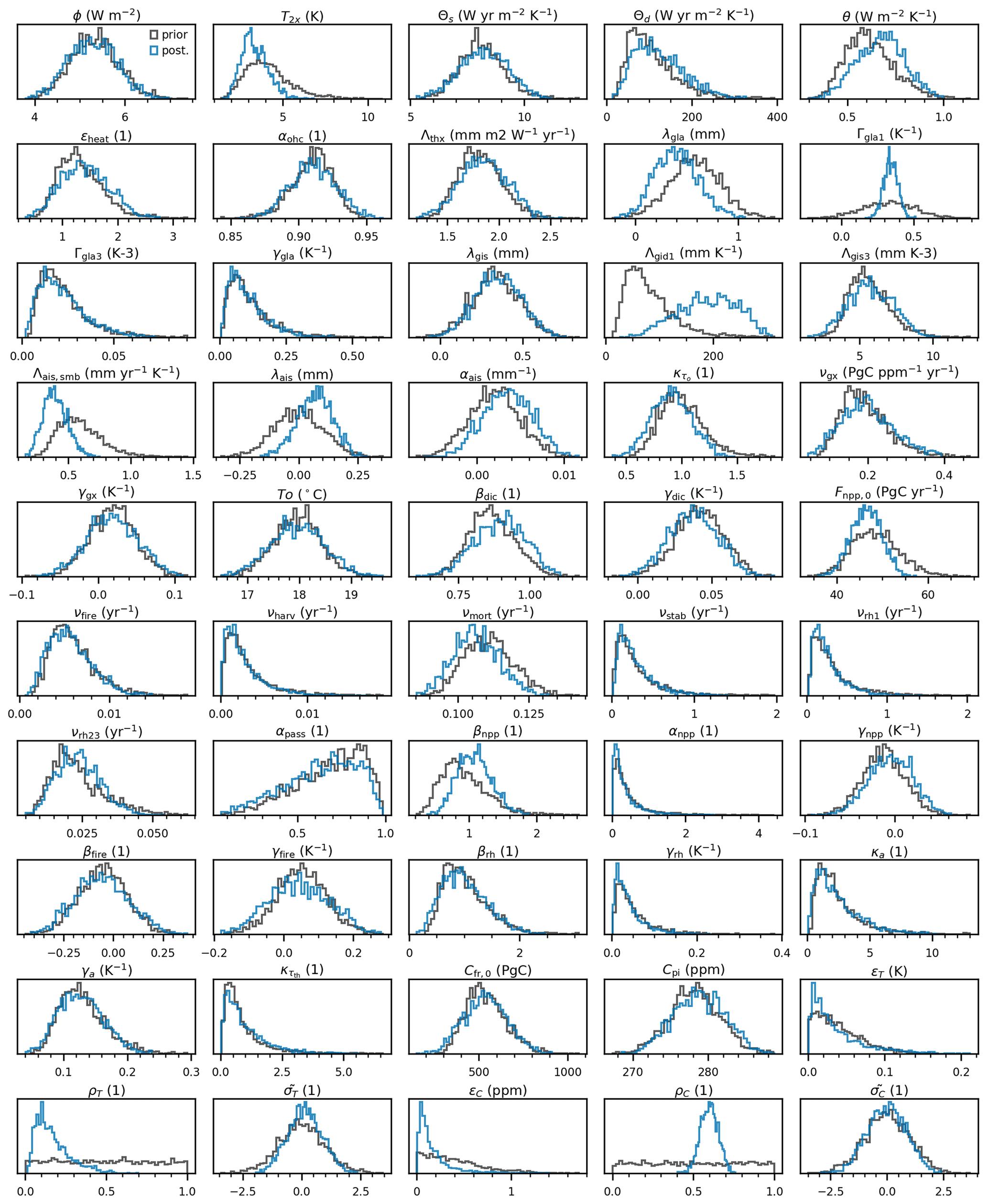
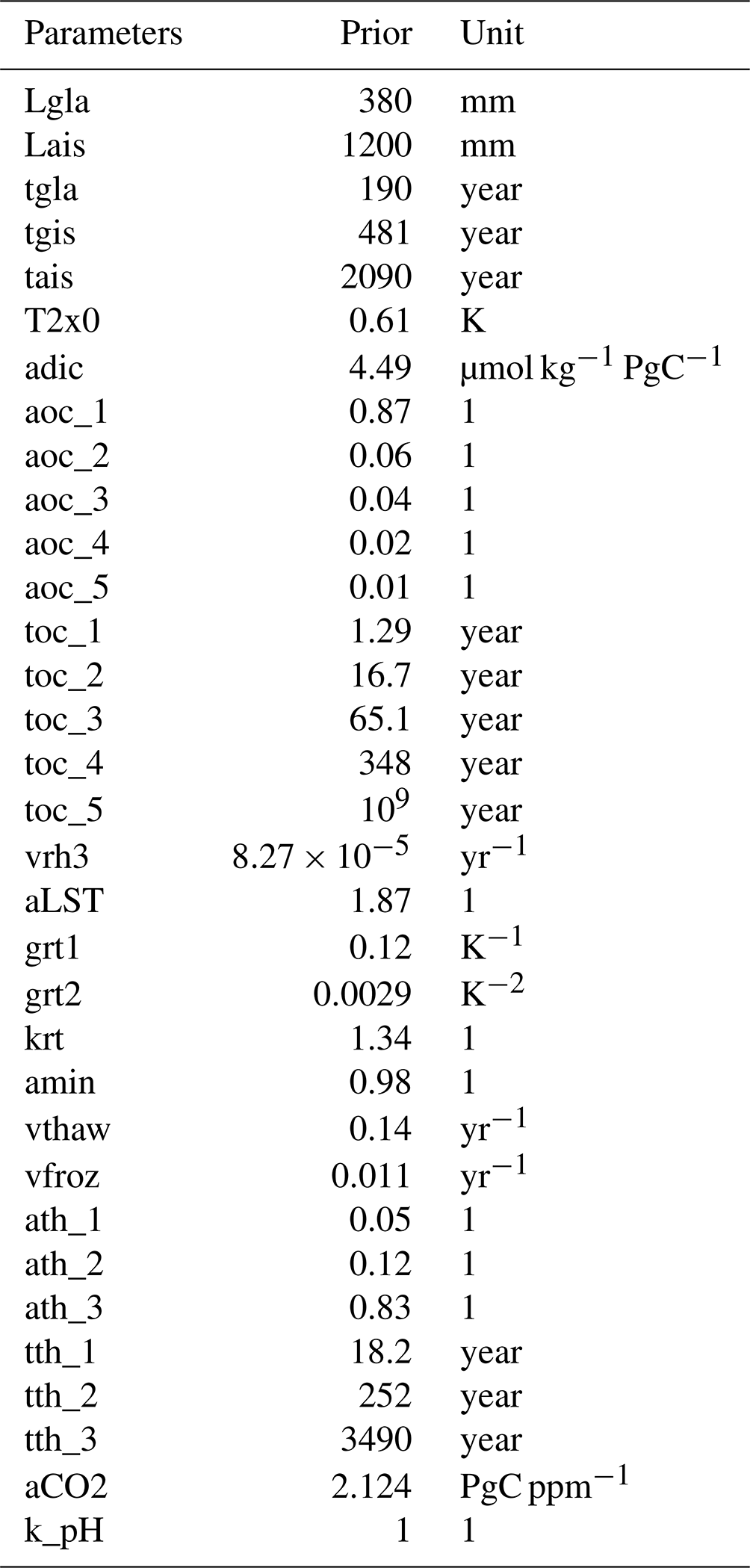
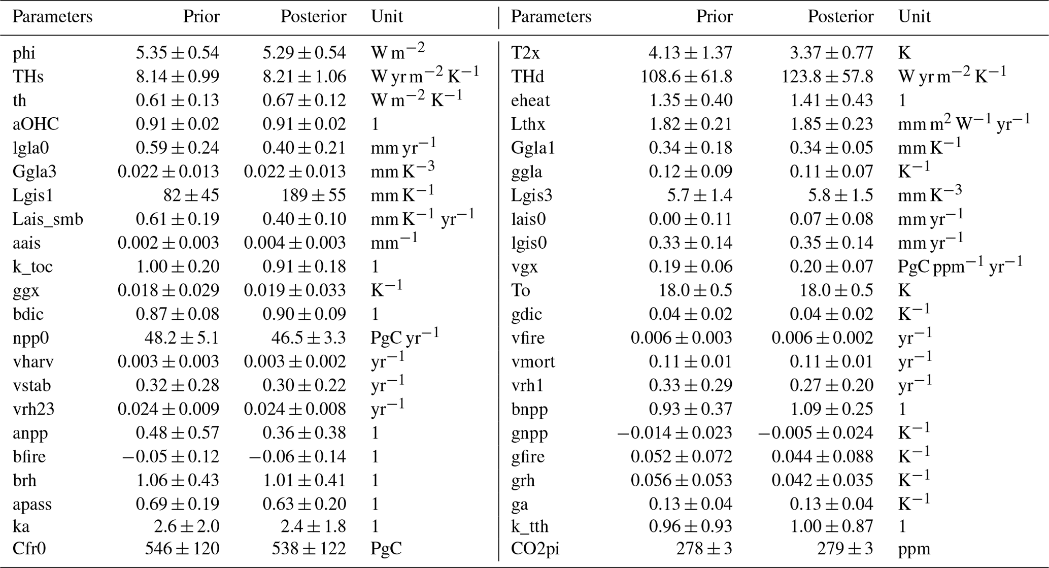
All parameters are summarized in Tables B5 and B6 along with their properties and values. The following subsections further explain how the prior distributions of the parameters are established, and these distributions are shown in Fig. 5.

Figure 5 Parameter distributions before (black lines) and after (blue lines) the Bayesian calibration. Parameters are noted under their text notation, and Tables B3 and B4 provide the corresponding notation in code.

3.4.1 Climate

All the parameters of the climate module are calibrated. The prior distribution of the radiative parameter ϕ is taken from the AR5 (Myhre et al., 2013, Table 8.SM.1). All other prior distributions of the parameters of the climate module (i.e. T_2×, Θ_s, Θ_d, θ, and ϵ_heat) are taken from 35 CMIP6 models whose climate responses were derived for the AR6 using the “abrupt-4xCO2” experiment (Smith et al., 2021, Sect. 7.SM.2.1, and corresponding GitHub repository). Here, T_2× is simply assumed to be half the reported equilibrium temperature at quadrupled CO₂. In addition, the prior distribution of the ocean warming fraction α_ohc is taken from the AR6 (Forster et al., 2021, Table 7.1).

3.4.2 Sea level rise

Some parameters from the SLR module are structural: the maximum SLR contribution from glaciers (Λ_gla) is taken from Fox-Kemper et al. (2021, Sect. 9.6.3.2); the equilibrium AIS SLR (Λ_ais) is from (Church et al., 2013, Fig. 13.14); and the τ_gis, τ_gla, and τ_ais timescales are the mean values from Mengel et al. (2016, Table S1) (assuming they provide the 90 % range of a log-normal distribution). All other parameters are calibrated. The prior distribution of the thermosteric parameter Λ_thx is taken from the AR6 (Fox-Kemper et al., 2021, Sect. 9.2.4.1), as are the prior distributions of the preindustrial offset parameters λ_gis, λ_gla and λ_ais (Fox-Kemper et al., 2021, earliest period of Table 9.5). For the remaining parameters, we derive prior distributions using SLR projections compiled by Edwards et al. (2021) for a number of ice sheets and glaciers models over various Representative Concentration Pathway (RCP) and Shared Socioeconomic Pathway (SSP) scenarios. Using the models' outputs, we apply Eq. (9) to estimate the Λ_gis1 and Λ_gis3 parameters; Eq. (10) for the Γ_gla1, Γ_gla3, and γ_gla parameters; and Eq. (12) for the Λ_ais,smb and α_ais parameters. During these fits, all other parameters are assumed to take their default value if structural, and their best-guess value otherwise. Results of this calibration on the individual models compiled by Edwards et al. (2021) are shown for each SLR contribution in Figs. B6, B7 and B8.

3.4.3 Ocean carbon

The ocean carbon cycle module has a number of structural parameters: α_dic, all α_o,j, and all τ_o,j are taken from Strassmann and Joos (2018, Tables A2 and A3, based on the Princeton model). The prior distribution of the adjustment factor ${\mathit{\kappa }}_{{\mathit{\tau }}_{\mathrm{o}}}$ is arbitrarily taken to apply a 20 % uncertainty on the oceanic transport timescales. All other prior distributions for this module's parameters are derived from 12 CMIP6 models with interactive carbon cycle that contributed to C4MIP (Arora et al., 2020). T_o is taken on average over the piControl simulation. ν_gx and γ_gx are calibrated by applying Eq. (18) to the models' outputs for the 1pctCO2, 1pctCO2-rad, and 1pctCO2-bgc experiments, while β_dic and γ_dic are calibrated by applying Eqs. (14)–(17) and (19). Results of this calibration on the individual CMIP6 models are shown in Figs. B1 and B2.

3.4.4 Ocean acidification

In this version of Pathfinder, κ_pH is a structural parameter set to 1.

3.4.5 Land carbon

Parameters related to the passive soil carbon pool are taken from He et al. (2016, Table S5): ν_rh3 is structural, while α_pass is not. All the prior distribution of the parameters related to the preindustrial steady state of the land carbon (i.e. F_npp0, ν_fire, ν_harv, ν_mort, ν_stab, ν_rh1, and ν_cs) are derived from 11 TRENDYv7 models (Sitch et al., 2015; Le Quéré et al., 2018), exactly as for OSCAR v3.1 (Gasser et al., 2020) except that all biomes and regions are lumped together. The prior distribution of the remaining parameters are derived from 12 CMIP6 models that contributed to C4MIP (Arora et al., 2020). Using the models' outputs for the 1pctCO2, 1pctCO2-rad, and 1pctCO2-bgc experiments, we calibrated β_npp, α_npp, and γ_npp through Eq. (24); β_fire and γ_fire through Eq. (28); and β_rh and γ_rh through Eq. (37). Results of this calibration on the individual CMIP6 models is shown in Figs. B3, B4, and B5.

3.4.6 Permafrost carbon

The permafrost module's parameters are recalibrated using the same algorithm as used by Gasser et al. (2018) but adapted to the global formulation of Pathfinder. First, the algorithm is run once to obtain a set of parameters reproducing the behaviour of the global average of five permafrost models (with data from UVic (MacDougall, 2021) added to the four original models). This gives the values of the structural parameters (i.e. α_lst, γ_rt1, γ_rt2, κ_rt, a_min, all α_th,j, all τ_th,j, ν_thaw, and ν_froz). Second, the algorithm is run five additional times for each of the five permafrost models separately, with the structural parameters established in the first step, to obtain prior distributions of the remaining parameters (i.e. C_fr0, κ_a, γ_a, and ${\mathit{\kappa }}_{{\mathit{\tau }}_{\mathrm{th}}}$).

3.4.7 Atmospheric CO₂

The conversion factor α_C is a structural parameter whose value is taken from the latest GCBs (e.g. Le Quéré et al., 2018). The prior distribution of preindustrial CO₂ concentration (C_pi) is taken from the AR6 (Gulev et al., 2021, Sect.  2.2.3.2.1), assuming the difference between minimum and maximum over the 0–1850 period is representative of the 90 % uncertainty range.

3.4.8 Historical CO₂ and GMST

The structural X_μ and X_σ time series are taken from the latest observations, as follows. T_μ and T_σ are taken as the average and standard deviation of five observational GMST data sets: HadCRUT5 (Morice et al., 2021), Berkeley Earth (Rohde et al., 2013; Rohde, 2013), GISTEMP (Hansen et al., 2010), NOAAGlobalTemp (Huang et al., 2020), and JMA (2022). We use the 1850–1900 period to define our preindustrial baseline, and GMST change is assumed to be zero before the earliest date available in each data set. Regarding atmospheric CO₂, C_μ is taken as the global value reported by NOAA/ESRL (Tans and Keeling, 2010) and C_σ as a constant ±1 ppm uncertainty for 1980 onward (this uncertainty is arbitrarily taken higher than the actual uncertainty estimated through instrumental measures to increase freedom in the calibration). Before that period, C_μ comes from the IPCC AR6 (Dentener et al., 2021, Table AIII.1a), and C_σ is linearly interpolated backwards from the instrumental uncertainty in 1980 to the preindustrial one (Gulev et al., 2021) in 1750. Finally, the prior distribution of ρ_X is set to uniform over [0,1], that of ${\stackrel{\mathrm{̃}}{\mathit{\sigma }}}_X$ is a unit normal distribution, and that of ϵ_X is set arbitrarily to a half-normal of parameter 0.05 K for GMST and 0.5 ppm for CO₂.

3.5 Results (posterior distributions)

The following subsections discuss the adjustments between the prior and posterior parameters that are the results of the Bayesian calibration, as well as the matching of the constraints. These sections constantly refer to Fig. 5 that shows the prior and posterior distributions of the model's parameters, Fig. 6 that shows those of the constrained variables, and Fig. 7 that displays the correlation matrix of the posterior parameters (there is no correlation among the prior parameters). Prior and posterior values of the parameters can also be retrieved from Table B6.

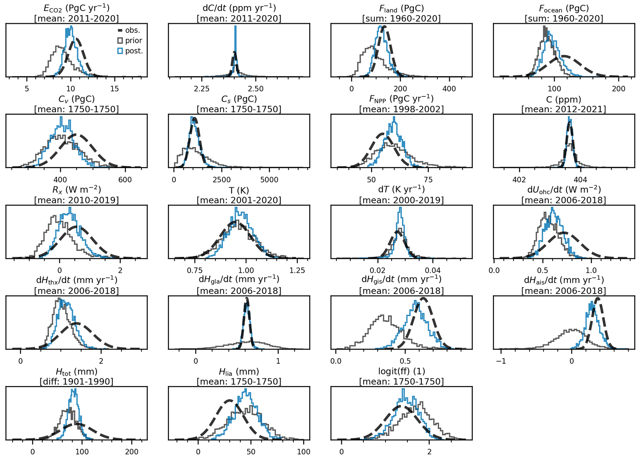
Figure 6 Distributions of the constrained variables. Dashed lines give the distributions used to constrain. Black lines give the distribution before calibration, while blue lines give the distribution posterior to calibration. Under a variable's name, we give the period over which the constraint is estimated and the data processing method: mean over the period, difference between last and first year, or sum of all the years over the period. (1750 is the preindustrial period). Variables are noted under their text notation, and Tables B1 and B2 provide the corresponding notation in code.

3.5.1 Climate system

Our climate-related constraints lead to adjusting all the parameters of the climate module. As explained in Sect. 3.4.8, the constraints for present-day GMST change and its derivative are met by construction.

The ECS (T_2×) is the parameter with the strongest adjustment, since it is directly constrained. Its precise value is discussed hereafter in Sect. 4.2, but we note that it is unsurprisingly decreased, as the CMIP6 model ensemble tends to overestimate the ECS compared to the IPCC-assessed value. Consequently, our posterior logit(ff) matches the constraint well. The adjustment of the ECS significantly reduces the gap between our posterior distribution of the non-CO₂ ERF and its constraint, although the posterior central value remains 41 % lower (but well within uncertainty range).

Among the dynamic parameters that are adjusted, we note that the deep-ocean heat capacity Θ_d is somewhat increased compared to the prior and that the heat exchange coefficient θ is also increased. These dynamic parameters are likely adjusted through our OHU constraint that is corrected in the posterior so the difference in the central values is lowered from 22 % to 14 %, which remains well within the uncertainty range.

Table 2 Diagnostics of climate and carbon cycle responses in Pathfinder before and after Bayesian calibration. Comparison with AR6 (Forster et al., 2021; Canadell et al., 2021) and CMIP6 data (Arora et al., 2020; Meehl et al., 2020) is shown. For AR6 data we give the median and 90 % confidence interval, while for every other value we give the mean ±1σ.

In addition, a number of weak but physically meaningful correlations across the climate module's parameters are found, such as a positive correlation between T_2× and ϵ_heat (see, e.g. Geoffroy et al., 2013a), a positive correlation between T_2× and Θ_d (that tends to exclude configuration that would warm fast and high), and a negative correlation between T_2× and ϕ (to match the GMST and ERF constraints together).

3.5.2 Carbon cycle

Similarly to GMST, the posterior distribution of atmospheric CO₂ concentration matches the constraint by construction. Its derivative, however, is (slightly overly) corrected to match the GCB estimate. Global anthropogenic CO₂ emissions are significantly increased to get closer to the GCB constraint, but their central value remains 9 % too low. Since these emissions are determined through mass balance and the atmospheric CO₂ matches observations, this implies that the total carbon sinks (i.e. F_land+F_ocean) must be weaker.

This is confirmed for the ocean sink, as the posterior central value of F_ocean is 8 % lower than the constraint but still noticeably corrected if compared to the prior. This correction is explained by small adjustments in some parameters of the ocean carbon module. The mixed-layer depth is slightly increased through β_dic. All other parameters remain mostly unaffected by the calibration, and only minor correlations are found. These results, along with the fact that our prior distribution spans only about half of the constraint's distribution, suggest that there is a structural limitation in our ocean carbon module that warrants further investigation.

It is also confirmed that the posterior land sink is weaker than the constraint, by 15 % for the central value, which is nevertheless a significant reduction of the prior gap of 34 %. To explain this adjustment, we observe that the CO₂ fertilization sensitivities (β_npp and γ_npp) are adjusted upwards. However, our constraint on present-day NPP prevents these adjustments from being too important, as the posterior distribution of this variable is similar to the prior and its central value remains 8 %–9 % higher than its constraint. An increased preindustrial NPP mechanically leads to an increase in preindustrial carbon pools, but these require further adjustments of the land carbon turnover rates, and most notably the mortality rate ν_mort and the passive carbon fraction α_pass, to better match their constraints (of which the one on total soil carbon is perfectly met).

Table 3 Comparison of SSP scenarios for GMST change projections (w.r.t. 1850–1900) to AR6 (Lee et al., 2021, Table 4.5), and for ocean and land carbon storage projections to CMIP6 (Liddicoat et al., 2021). Land carbon storage projections were corrected using the land use change emissions data from SSPs (Riahi et al., 2017; Gidden et al., 2019). For GMST data we give the median and the 90 % confidence interval while for every other values we give the mean ±1σ.

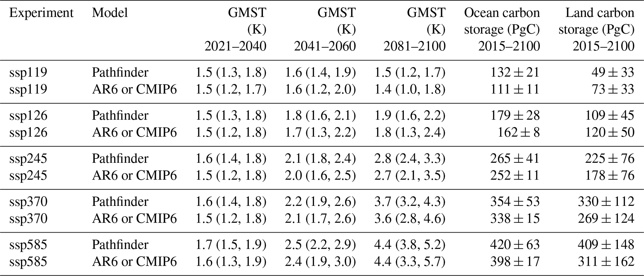
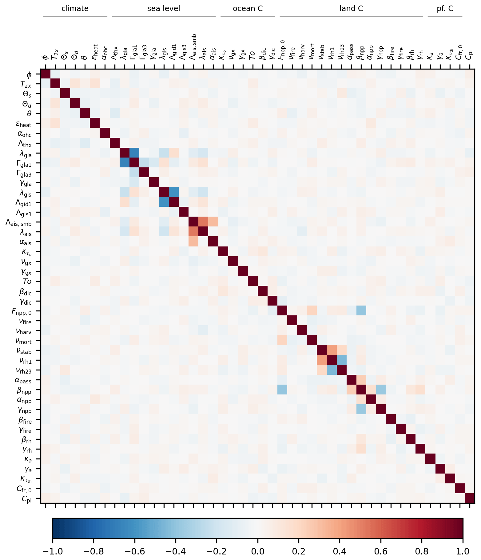
Figure 7 Correlation matrix of Pathfinder's parameters after the Bayesian calibration. Parameters are classified according to the equations they are related to, i.e. climate system, sea level, ocean carbon, land carbon, and permafrost carbon. Parameters are noted under their text notation, and Tables B3 and B4 provide the corresponding notation in code.

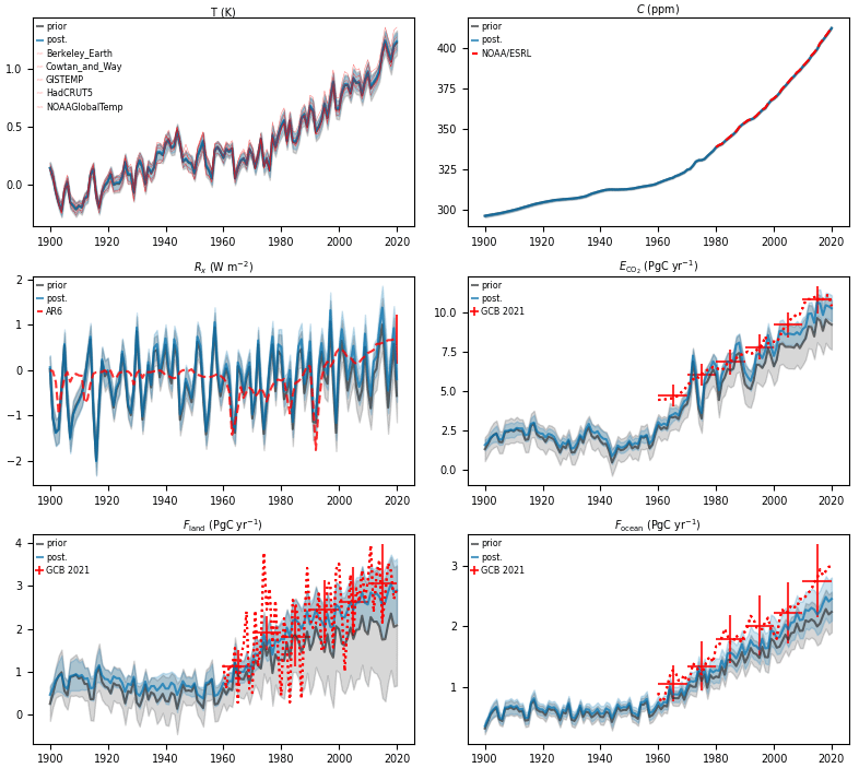
Figure 8 Historical time series of key variables from Pathfinder. Red lines are observations, black lines are the model's outputs before calibration, and blue lines are the same after calibration. Shaded areas and vertical bars correspond to the 1σ uncertainty range. Temperature observations are taken from HadCRUT5 (Morice et al., 2021), Cowtan and Way (2014), Berkeley Earth (Rohde et al., 2013; Rohde, 2013), GISTEMP (Hansen et al., 2010), and NOAA/MLOST (Vose et al., 2012). Other sources are NOAA/ESRL (Tans and Keeling, 2010), GCB 2021 (Friedlingstein et al., 2022), and AR6 (Smith et al., 2021).

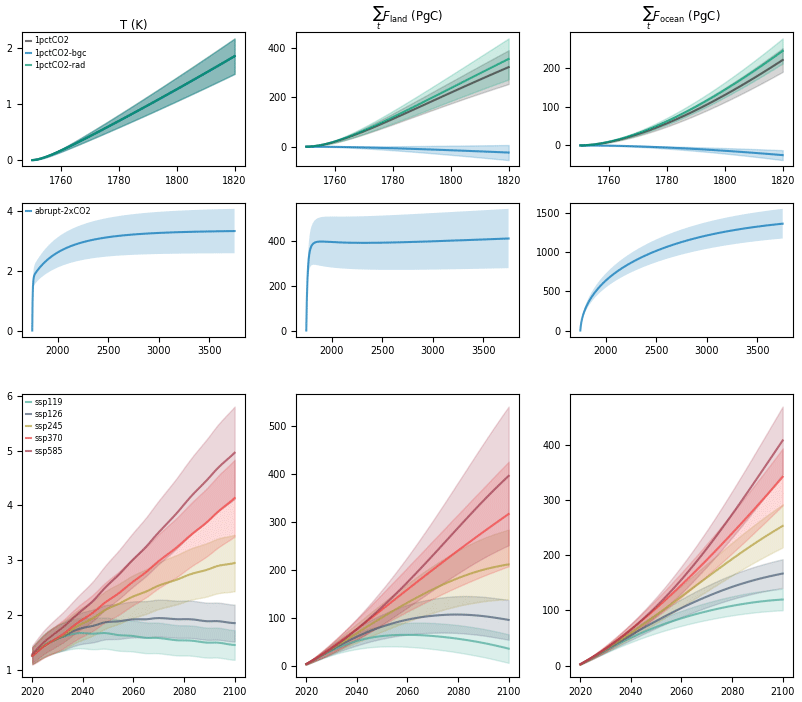
Figure 9 Time series of GMST change, integrated land carbon uptake and integrated ocean carbon uptake for idealized experiments (abrupt-2xCO2, 1pctCO2, 1pctCO2-bgc and 1pctCO2-rad) and projections according to SSP scenarios in Pathfinder. Shaded areas give the 1σ uncertainty range.

The land carbon module exhibits significant correlations among posterior parameters. This is likely a consequence of all the constraints combined as they dictate both the preindustrial steady state of the module and its transient response over the historical period. Eliminated configurations are those, for instance, that would show high initial carbon pools that are very sensitive to climate change (as these would lead to a very weak land sink) or that would exhibit a weak CO₂ fertilization effect associated with a fast turnover time (that would also lead to a weak sink).

3.5.3 Sea level rise

The prior parameters of the SLR module are the least informed of our Bayesian setup. The model initially underestimates the thermal expansion, as well as the GIS and AIS SLR rates. The calibration brings the posterior distributions closer to their respective constraints but it always remains in the lower end of the uncertainty range. The correction is done by adjusting many of the module's parameters (most notably Λ_gis1, Λ_ais,smb, λ_ais or λ_gla) and by finding strong correlations among them (thus excluding physically unrealistic combinations).

The historical SLR is markedly corrected by the constraint: from a 19 % gap between the central values of the constraint and the prior estimate, to only 7 % after calibration. Here, we also note that the sum of individual contributions to historical SLR reported in AR6 do not match that total SLR (Fox-Kemper et al., 2021, Table 9.5), which likely has some impact on the consistency between our constraints. Finally, although the LIA relaxation contribution is not altered by the calibration, as its central value remains 50 % too high, it is the likely source of the strong correlations found among the parameters of this module because it straightforwardly links the individual SLR contributions together.

4 Model diagnosis

4.1 Historical period

Because in the Bayesian setup we do not use annual time series of observations as constraints, the posterior distributions given in Fig. 6 do not inform on the whole dynamic of the model over the historical period. To further diagnose the model's behaviour, Fig. 8 gives the time series from 1900 to 2021 of six key variables. GMST and atmospheric CO₂ match the historical observations very well via construction of these input time series. The non-CO₂ ERF exhibits a very high variability, owing to our temperature-driven setup and the natural variability in the GMST input. Beyond that, the ERF time series is consistent with the AR6 estimates (Smith et al., 2021), albeit somewhat lower on average in the recent past, as seen with the posterior distribution. Consistently with the interpretation of carbon cycle variables in the calibration results, anthropogenic CO₂ emissions, and the ocean and land carbon sinks are slightly underestimated compared to the GCB estimates (Friedlingstein et al., 2022). Several reasons could explain this discrepancy, from the lack of land use change in Pathfinder to the inconsistency of the GCB figures (that do not close the budget, while ours do). Nevertheless, the interest of the calibration is clearly illustrated, as the posterior uncertainty range covers observations much better than the prior one.

4.2 Idealized simulations

To complete the diagnosis of our model with common metrics used with climate and carbon models, we ran a set of standard idealized experiments, corresponding to the CMIP6 abrupt-2xCO2, 1pctCO2, 1pctCO2-bgc, and 1pctCO2-rad. A summary of these metrics' values is given in Table 2, and the resulting time series are shown in Fig. 9.

The abrupt-2xCO2 experiment sees an abrupt doubling of atmospheric CO₂, and it is used to diagnose the model's ECS that is defined as the equilibrium temperature for a doubling of the preindustrial atmospheric concentration of CO₂ (we acknowledge that it is superfluous with this version of Pathfinder since it is also a parameter). Using the GMST anomaly at the end of 1500 years of this experiment leads to an unconstrained estimate of ECS of 4.1 ± 1.3 K and a constrained estimate of 3.3 ± 0.7 K. Consistently, the latter value is between the ECS value extracted from CMIP6 models (Meehl et al., 2020) that is higher (3.7 ± 1.1 K) and the final value assessed in the AR6 that is lower (3.0 K, with a 67 % confidence interval between 2.5 and 4.0 K).

Using the 1pctCO2 experiment that sees a 1 % yearly increase in atmospheric CO₂, we can estimate the model's transient climate response (TCR), which is defined as the GMST change after 70 years, when atmospheric concentration CO₂ has just doubled. The CMIP6 models have a TCR of 2.0 ± 0.4 K (Meehl et al., 2020). Pathfinder's unconstrained value is higher, at 2.2 ± 0.5 K, while the constrained one goes down to 1.9 ± 0.3 K. If we divide the TCR by the cumulative anthropogenic CO₂ emissions compatible with the atmospheric CO₂ increase in this experiment, we obtain an estimate of the transient climate response to emissions (TCRE). Similarly to the TCR, it is higher in the unconstrained ensemble and lower in the constrained one, when compared to CMIP6 models (Arora et al., 2020). Both downward adjustments of the TCR and TCRE are consistent with that of ECS, with the posterior TCRE matching the AR6 assessed range very well (Canadell et al., 2021).

To look more closely at the carbon cycle, we perform two variants of the latter experiment: in 1pctCO2-rad, atmospheric CO₂ only has a radiative effect, as it is kept at preindustrial level for the carbon cycle, whereas in 1pctCO2-bgc, atmospheric CO₂ only has a biogeochemical effect, as the climate system sees only the preindustrial level. These three experiments are used to calculate the carbon–concentration (β) and carbon–climate (γ) feedback metrics that measure the carbon sinks' sensitivities to changes in atmospheric CO₂ and GMST, respectively. We apply the same method as Arora et al. (2020) to calculate these, which leads to metrics at the time of CO₂ doubling that are in line with CMIP6 models (Arora et al., 2020). As both carbon sinks were adjusted upwards by the Bayesian calibration, the constraints logically increased both β_ocean and β_land, to values fairly close to those of the complex models. The γ_ocean is not affected by the calibration and remains 45 % too low, which again suggests a structural limitation in our formulation of the ocean sink. This is, however, compensated for during calibration by the γ_land being 26 % higher than in complex models.

4.3 Scenarios

To further validate Pathfinder, we run the five SSP scenarios (Riahi et al., 2017) for which climate and carbon cycle projections were reported by a large enough number of models in the AR6 (namely, ssp119, ssp126, ssp245, ssp370, and ssp585). These simulations are run with prescribed CO₂ concentration and non-CO₂ ERF (the latter is taken from Smith et al., 2021). Time series of GMST and cumulative land and ocean sinks are shown in Fig. 9. Table 3 shows a comparison of the projected changes in GMST to the CMIP6 estimates (Lee et al., 2021, Table 4.2) and of carbon pools to Liddicoat et al. (2021) (since this was not directly reported in the AR6).

Be it on short-, mid- or long-term scales, Pathfinder's projections of GMST are very much in line with the one assessed by the IPCC in the AR6 based on multiple lines of evidence (Lee et al., 2021, Table 4.5). The only significant difference is a smaller uncertainty range in our projections for the longer-term periods. Although this is the result of the efficiency of the Bayesian calibration, one might wonder whether the climate module is over-constrained (or equivalently, too limited in its number of parameters).

The ocean carbon storage appears to be overestimated by 5 % to 20 % by Pathfinder across SSP scenarios. This is consistent with the upward adjustment of the ocean carbon sink stemming from our Bayesian calibration. To compare the land carbon storage with CMIP6 models, because our land carbon module does not include land use change processes, we correct the value reported by complex models by the cumulative land use change emissions of each scenario (Riahi et al., 2017; Gidden et al., 2019). While the land carbon storage of Pathfinder is well in line under ssp126 (a scenario consistent with the 2 ^∘C target), it is underestimated in ssp119 (consistent with the 1.5 ^∘C target) and increasingly overestimated in higher warming scenarios. A likely explanation is that the climate–carbon feedback on land is underestimated in Pathfinder, as suggested by the γ metric seen in Sect. 4.2. Alternatively (or concurrently), the absence of loss of sink capacity caused by land cover change (Gasser and Ciais, 2013; Gasser et al., 2020) can explain the overestimation of the land sink under high CO₂. The Pathfinder model's estimates of both sinks nonetheless remain well within the CMIP6 models' uncertainty ranges.

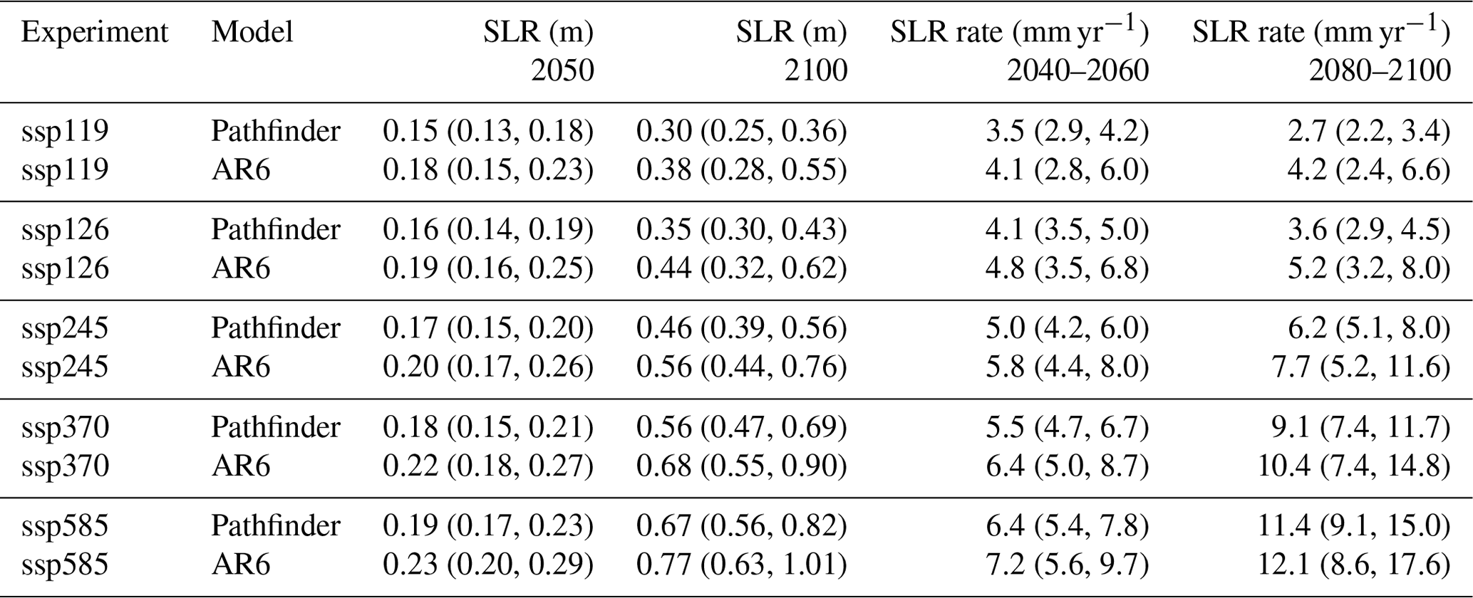
Our SLR emulator gives estimates (Table 4) that are always on the lower end of the range reported in the AR6 (Fox-Kemper et al., 2021, Table 9.9). This can be explained by the fact that our individual SLR rate estimates are on the lower end of their respective constraints (see Sect. 3.5.3). This discrepancy also highlights potential structural limitations in the SLR module (e.g. too few separate contributions) and the difficulty of calibrating the module given the short time period of data available, both from complex models (that cover the 21st century only) and observations, compared to the long timescale of the SLR processes. Nevertheless, our estimates remain within the uncertainty range of the IPCC assessment, especially as we do not account for contribution from land water storage that causes an additional 0.03 [0.01, 0.04] m of SLR in all scenarios in 2100 (Fox-Kemper et al., 2021).

Table 4 Comparison of SSP scenarios between Pathfinder and AR6 for SLR (with respect to 1995–2014) and SLR speed projections (Fox-Kemper et al., 2021, Table 9.9). We give the median value and the 90 % confidence interval in parentheses.

5 Concluding remarks

In this paper, we have presented the Pathfinder model: a simple global carbon–climate model with selected impact variables, carefully designed to balance accuracy of representation and simplicity of formulation and calibrated through Bayesian inference on the latest data from Earth system models and observations. Pathfinder has been shown to perform very well in comparison to complex models, although there remains room for further improvement of the model and its calibration setup. We identify four main avenues to improve the model.

First, some parts of the model may well lean too much on the complexity side of the simplicity–accuracy balance we aimed to strike, owing to the creation process of Pathfinder that mostly compiled existing formulations. Future development should therefore strive to reduce complexity wherever possible. The ocean carbon sub-pools and perhaps the land carbon pools are potential leads in this respect.

Second, the ocean carbon module alone appears to be limited by its structure, which has been inherited from a 25-year-old (yet seminal) article (Joos et al., 1996). Although it is undoubtedly a significant undertaking, developing an alternative formulation of the ocean carbon dynamic, calibrated on state-of-the-art ocean models and properly connected to ocean pH and the ocean of the climate module, would benefit more than just the SCM community.

Third, integration of land use and land cover change in such a model appears warranted, despite the difficulty of doing so in a physically sensible yet simple manner. Given our expertise with the OSCAR model and its bookkeeping module (Gasser et al., 2020), we are confident that this can be done, although it will demand extra care to keep the model compatible with the IAMs it is also meant to be linked to.

Fourth, the Bayesian setup can be extended, notably by including more time periods for the existing constraints but also by introducing and constraining entirely new variables such as isotopic ratios (Hellevang and Aagaard, 2015) or inter-hemispheric gradients (Ciais et al., 2019); however, a balance must be struck with respect to the calibration's computation time. Here, we caution against including complex models' results as constraints in the Bayesian calibration, as was done for the IPCC AR6 (Smith et al., 2021; Nicholls et al., 2021), as it goes against the philosophy of Pathfinder to use complex models' results as prior information only.

Fifth, although our model is restricted to CO₂ by design because of how IAMs like DICE (Nordhaus, 2017) are also limited to CO₂ emissions, we can imagine many reasons why one would want to add non-CO₂ climate forcers into Pathfinder. We would suggest doing so by following the model's philosophy: that is, by taking existing reduced-complexity formulations such as something between FaIR (Leach et al., 2020) and OSCAR (Gasser et al., 2017) and adding the new parameters into the Bayesian setup with the relevant observational constraints.

In spite of these few shortcomings and potential development leads, Pathfinder v1.0.1 is a powerful tool that fits the niche it has been created for perfectly. We will further demonstrate the strengths and flexibility of Pathfinder in other publications. Meanwhile, we invite the community to seize this open-source model and use it in any study that could benefit from a simple, fast, and accurate carbon–climate model aligned with the latest climate science.

Appendix A: Additional information about the model

A1 Technical requirements

Pathfinder has been developed and run in Python (v3.7.6) (https://docs.python.org/3.7/, last access: 5 December 2022), preferentially using IPython (v7.19.0) (Pérez and Granger, 2007). Currently, packages required to run it are NumPy (v1.19.2) (Harris et al., 2020), SciPy (v1.5.2) (Virtanen et al., 2020), and Xarray (v0.16.0) (Hoyer and Hamman, 2017), and it has hard-coded dependencies on PyMC3 (v3.8) (Salvatier et al., 2016) and Theano (v1.0.4) (Theano Development Team, 2016) that are in fact used only for calibration. Other versions of Python or these packages were not tested.

The calibration procedure takes about 9 h to run on a desktop computer (with a base speed of 3.4 GHz). Simple use of the model is much faster: the idealized experiments and SSP scenarios for this description paper, which represent 2984 simulated years, were run in about 20 min for all 2000 configurations and on a single core. A single simulated year takes a few tenths of a second, although a number of options in the model can drastically alter this performance. Note also that this scales sub-linearly with the amount of configurations or scenarios because of the internal workings of the Xarray package, albeit at the cost of increased demand in random-access memory.

A2 Known issues

Two relatively benign issues that have been identified during development remain unsolved. First, the model requires a high number of sub-time steps (i.e. high n_t) to remain stable under high CO₂ because of the ocean carbon cycle. Second, the version of the model that is driven by T and R_x time series is extremely sensitive to its inputs because it mathematically requires the first two derivatives of T and the first derivative of R_x.

A3 Changelog

Brief description of the successive versions of Pathfinder.

v1.0.1.

Exact same physical equations and numerical values as v1.0. Added best-guess parameters calculated as the average of the posterior distribution, and corresponding historical outputs, for single-configuration runs. Improved README and MANUAL files.

v1.0.

First release. Exact model described in the preprint version of this paper (Bossy et al., 2022).

Appendix B: Additional figures and tables

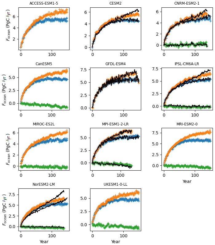
Figure B1 Calibration to estimate prior ν_gx and γ_gx from CMIP6 time series of F_ocean. We fit our equation on the results of the +1 % CO₂ (1pctCO2) experiment (in blue) and its variants 1pctCO2-rad (in green) and 1pctCO2-bgc (in orange). Coloured markers are CMIP6 model data, while the solid black lines show the fit from Pathfinder. Panels without a black line indicate that at least one of the required variables was not reported by the complex model.

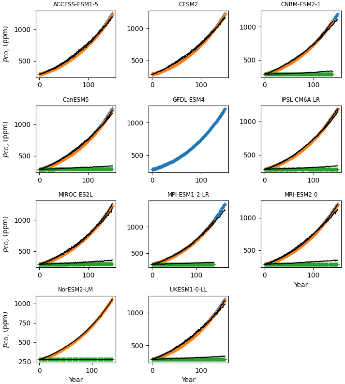
Figure B2 Calibration to estimate prior β_dic and γ_dic from CMIP6 time series of $p_{{\mathrm{CO}}_{\mathrm{2}}}$. We fit our equation on the results of the +1 % CO₂ (1pctCO2) experiment (in blue) and its variants 1pctCO2-rad (in green) and 1pctCO2-bgc (in orange). Coloured markers are CMIP6 model data, while the solid black lines show the fit from Pathfinder. Panels without a black line indicate that at least one of the required variables was not reported by the complex model.

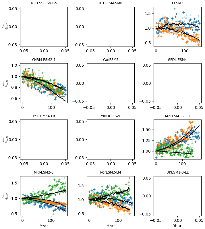
Figure B3 Calibration to estimate prior β_ef and γ_ef from CMIP6 time series of r_fire, shown as a ratio over its preindustrial value. We fit our equation on the results of the +1 % CO₂ (1pctCO2) experiment (in blue) and its variants 1pctCO2-rad (in green) and 1pctCO2-bgc (in orange). Coloured markers are CMIP6 model data, while the solid black lines show the fit from Pathfinder. Panels without a black line indicate that at least one of the required variables was not reported by the complex model.

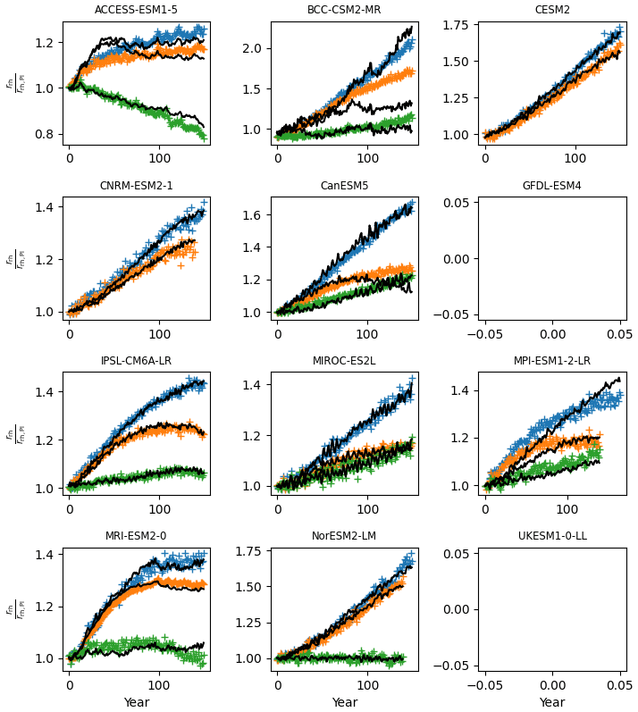
Figure B4 Calibration to estimate prior β_rh and γ_rh from CMIP6 time series of r_rh, shown as a ratio over its preindustrial value. We fit our equation on the results of the +1 % CO₂ (1pctCO2) experiment (in blue) and its variants 1pctCO2-rad (in green) and 1pctCO2-bgc (in orange). Coloured markers are CMIP6 model data, while the solid black lines show the fit from Pathfinder. Panels without a black line indicate that at least one of the required variables was not reported by the complex model.

Figure B5 Calibration to estimate prior β_npp, α_npp, and γ_npp from CMIP6 time series of r_npp, shown as a ratio over its preindustrial value. We fit our equation on the results of the +1 % CO₂ (1pctCO2) experiment (in blue) and its variants 1pctCO2-rad (in green) and 1pctCO2-bgc (in orange). Coloured markers are CMIP6 model data, while the solid black lines show the fit from Pathfinder. Panels without a black line indicate that at least one of the required variables was not reported by the complex model.

Figure B6 Calibration to estimate the prior of GIS SLR module parameters (Λ_gis1, Λ_gis3, and λ_gis0). We fit our equation on the compiled outputs from Edwards et al. (2021) for which there is more than one scenario available. Each panel's title displays the name of the institute, model, and configuration used. Coloured markers are the model data, while the solid black lines show the fit from Pathfinder.

Figure B7 Calibration to estimate the prior of glacier SLR module parameters (Γ_gla1, Γ_gla3, γ_gla, and λ_gla0). We fit our equation on the compiled outputs from Edwards et al. (2021) for which there is more than one scenario available. Each panel's title displays the name of the model or study used. Coloured markers are the model data, while the solid black lines show the fit from Pathfinder.

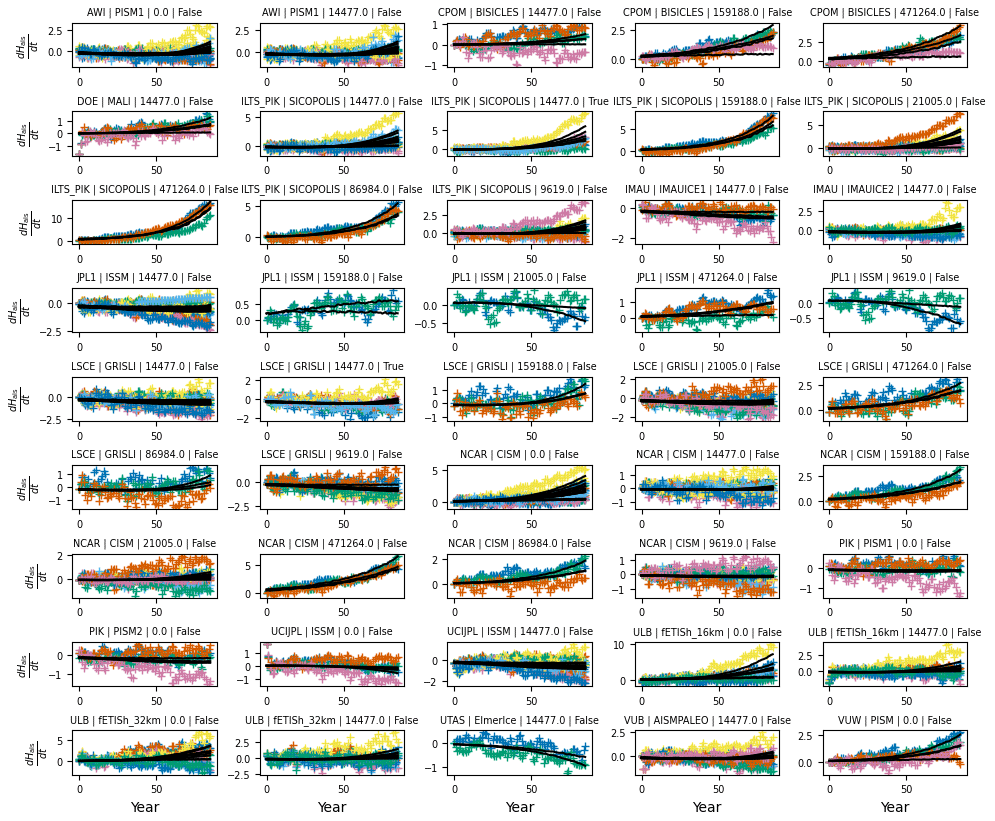
Figure B8 Calibration to estimate the prior of AIS SLR module parameters (Λ_ais,smb, α_ais, and λ_ais0). We fit our equation on the compiled outputs from Edwards et al. (2021) for which there is more than one scenario available. Each panel's title displays the name of the institute, model and configuration used. Coloured markers are the models data while the solid black lines show the fit from Pathfinder.

Figure B9 Distribution of the logit of the ECS (T_2×) inferred from AR6. Blue points are the assessments from AR6, the solid line is the cumulative distributive function (CDF) fitted on those assessments, and the dashed line is the PDF associated with the CDF (arbitrary scale). The value of the fitted parameters is given above the plot.

Table B1 Summary of Pathfinder's equation variables in climate, sea level, and ocean carbon modules.

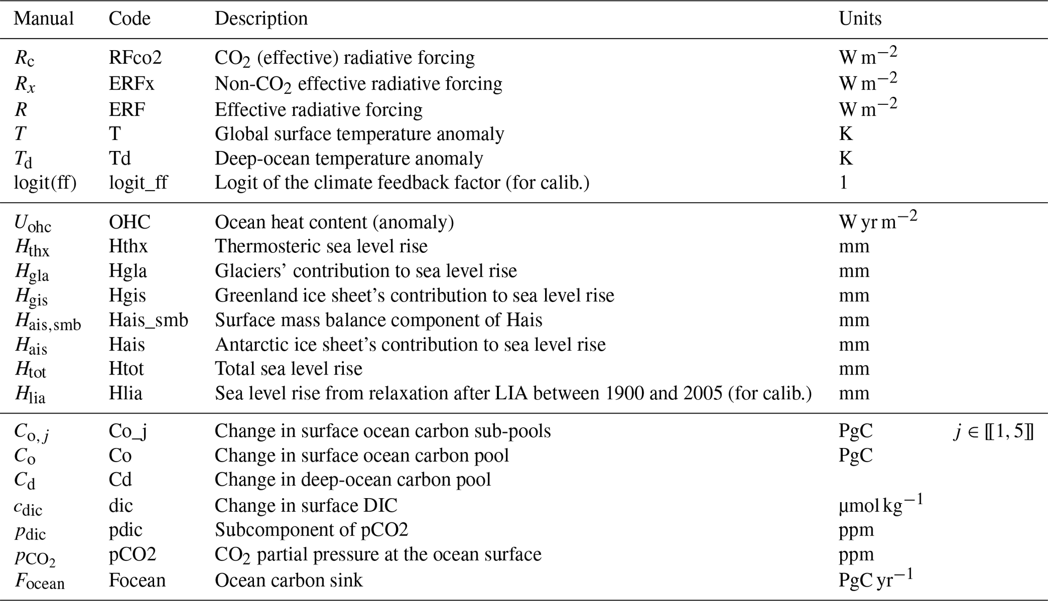
Table B2 Summary of Pathfinder's equation variables for land carbon, permafrost, and atmospheric modules.

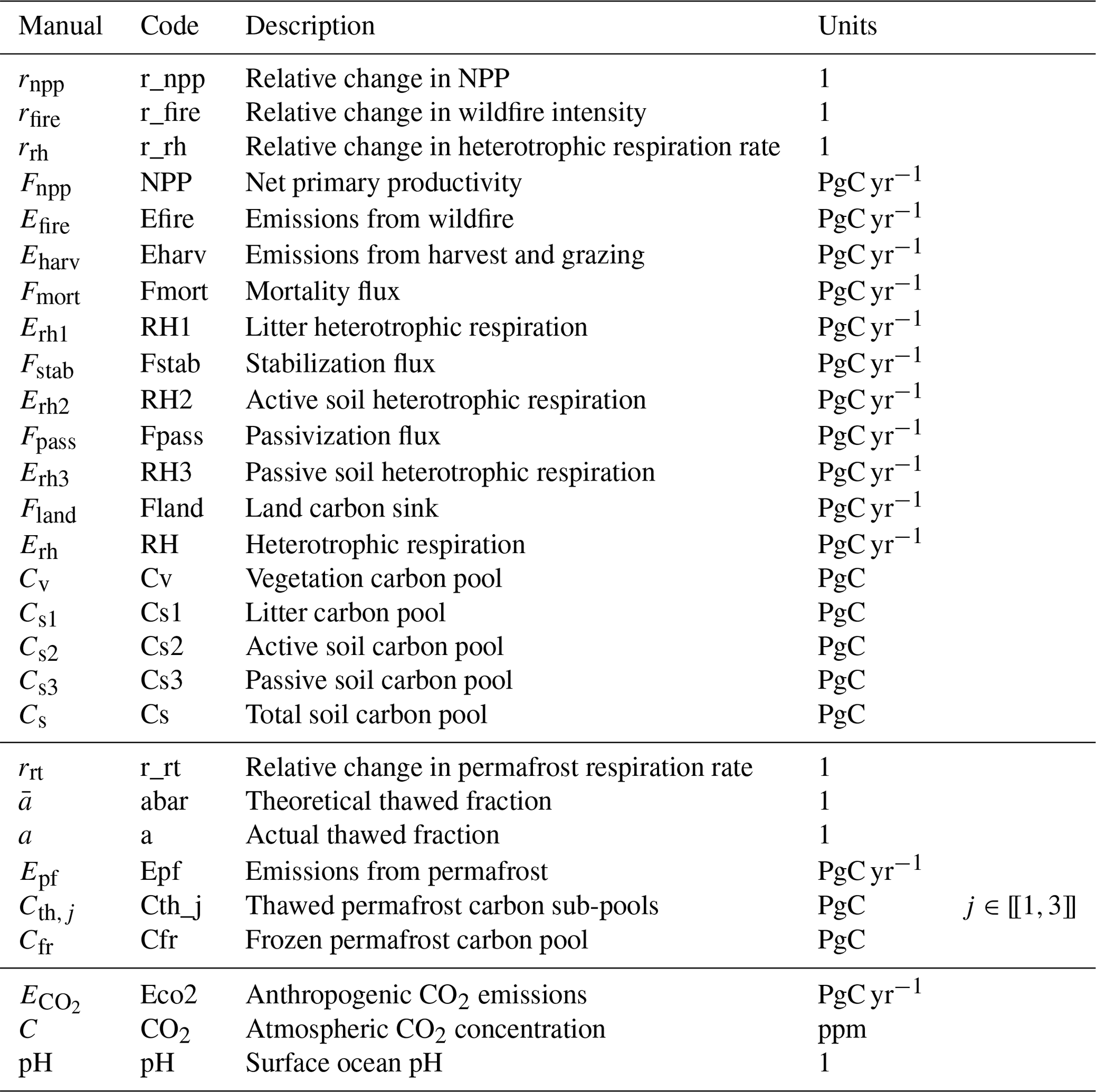
Table B3 Parameters used in the climate, ocean carbon, and sea level modules.

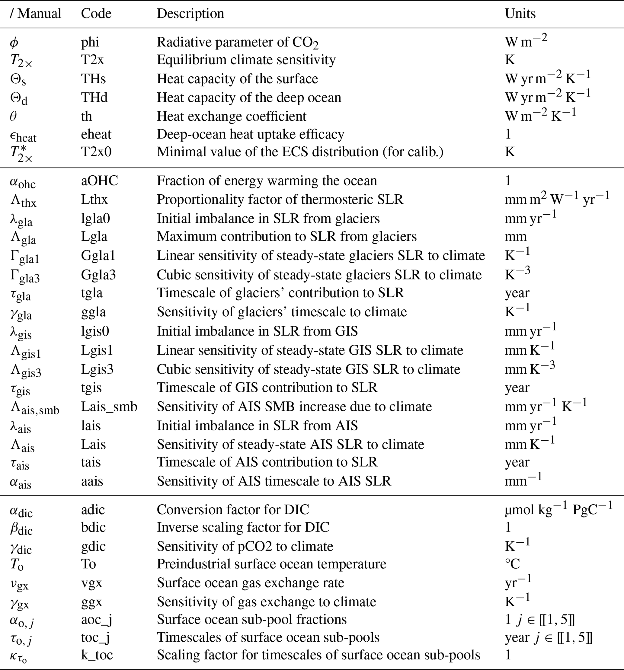
Table B4 Parameters used in the permafrost, land carbon modules, and for calibration.

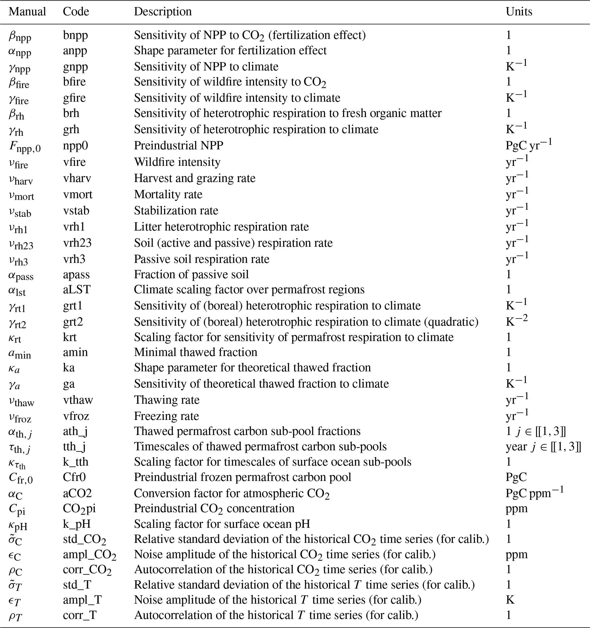
Table B5 Structural parameter values. Parameters are noted under their code notation, and Tables B3 and B4 provide the corresponding notation in text.

Table B6 Calibrated parameter values before and after Bayesian calibration. Parameters are noted under their code notation, and Tables B3 and B4 provide the corresponding notation in text. The uncertainty corresponds to the 1σ uncertainty range.