Basin-scale gyres and mesoscale eddies in large lakes: a novel procedure for their detection and characterization, assessed in Lake Geneva

In large lakes subject to the Coriolis force, basin-scale gyres and mesoscale eddies, i.e. rotating coherent water masses, play a key role in spreading biochemical materials and energy throughout the lake. In order to assess the spatial and temporal extent of gyres and eddies, their dynamics and vertical structure, as well as to validate their prediction in numerical simulation results, detailed transect field observations are needed. However, at present it is difficult to forecast when and where such transect field observations should be taken. To overcome this problem, a novel procedure combining 3D numerical simulations, statistical analyses, and remote sensing data was developed that permits determination of the spatial and temporal patterns of basin-scale gyres during different seasons. The proposed gyre identification procedure consists of four steps: (i) data pre-processing, (ii) extracting dominant patterns using empirical orthogonal function (EOF) analysis of Okubo–Weiss parameter fields, (iii) defining the 3D structure of the gyre, and (iv) finding the correlation between the dominant gyre pattern and environmental forcing. The efficiency and robustness of the proposed procedure was validated in Lake Geneva. For the first time in a lake, detailed field evidence of the existence of basin-scale gyres and (sub)mesoscale eddies was provided by data collected along transects whose locations were predetermined by the proposed procedure. The close correspondence between field observations and detailed numerical results further confirmed the validity of the model for capturing large-scale current circulations as well as (sub)mesoscale eddies. The results also indicated that the horizontal gyre motion is mainly determined by wind stress, whereas the vertical current structure, which is influenced by the gyre flow field, primarily depends on thermocline depth and strength. The procedure can be applied to other large lakes and can be extended to the interaction of biological–chemical–physical processes.

1 Introduction

Pressure on large lakes, as major freshwater resources, is increasing due to a combination of changing climate and human activities. To a large extent, lake water quality is controlled by the pathways along which nutrients, phytoplankton, and contaminants are transported/redistributed on mesoscales or basin scales (Mahadevan, 2016; Ralph, 2002); in this context, gyres and eddies play an important role. Basin-scale gyres are usually restricted in the vertical by the thermocline depth (Ishikawa et al., 2002; Ji and Jin, 2006), which is also subject to high spatial and temporal variability due to the presence of mesoscale or submesoscale circulations (Nõges and Kangro, 2005; Ostrovsky and Sukenik, 2008; Corman et al., 2010).

Understanding gyre dynamics in large lakes has mainly been advanced by Csanady's theoretical analyses (Csanady, 1973, 1975). Wind forcing (the primary driver), the Earth's rotation (Coriolis force), and lakebed morphology are the main controlling parameters (Birchfield, 1967; Rao and Murty, 1970; Csanady, 1973; Pickett and Rao, 1977; Rueda et al., 2005; Shimizu et al., 2007; Nakayama et al., 2014). In order to provide and accumulate enough energy to generate basin-scale circulations such as gyres, wind with a relatively constant direction must blow over most of the water surface for a certain time (Csanady, 1975). It has been shown that in the Laurentian Great Lakes in North America, a downwind flow in shallower nearshore regions and an upwind return flow in the deeper part of a lake basin enhance the formation of such circulation cells. Stratification and the width of downwind flow, which is also known as a “coastal jet,” will increase and confine the flow to the surface layer (Bennett, 1974). However, these studies were conducted under simplified boundary conditions, using bathymetry and atmospheric forcing data with limited resolution.

Theoretical studies have indicated that the response of a depth-variable lake to a strong uniform wind often leads to the formation of two counter-rotating gyres, also known as a double gyre or dipole (Csanady, 1973; Bennett, 1974; Shilo et al., 2007), as was confirmed by early numerical simulations (Simons, 1980). With increased computational power, three-dimensional (3D) hydrodynamic models with higher accuracy, stability, and resolution have since been developed and have significantly contributed to the understanding of lake circulation, especially that driven by wind (e.g. Beletsky et al., 1999; Laval et al., 2005; Beletsky and Schwab, 2008; Bai et al., 2013; Mao and Xia, 2020; Baracchini et al., 2020a; Lin et al., 2022; Wu et al., 2022). Recent numerical simulations have also highlighted the role of baroclinicity induced by gradients of surface buoyancy (mainly surface heating and cooling), which can enhance the large-scale circulation in the Great Lakes (Schwab and Beletsky, 2003; Bennington et al., 2010; Verburg et al., 2011; McKinney et al., 2012).

Based on long-term current data of the Laurentian Great Lakes from a limited number of moorings, Beletsky et al. (1999) suggested that during the non-stratified season, a single anticlockwise-rotating gyre exists in larger lakes (Lake Huron, Lake Michigan, Lake Superior), whereas a two-gyre pattern is established in smaller ones (Lake Ontario, Lake Erie). Stratification can modify this pattern. A two-gyre pattern was also observed in Lake Okeechobee (USA), a shallow (3.2 m mean depth) large lake (Ji and Jin, 2006). In Lake Biwa (Japan), topography, stratification, and non-linearity were found to affect gyre development and could result in a three-gyre pattern (Akitomo et al., 2004). Determining the direct influence of atmospheric forcing on individual large-scale current systems in large lakes is challenging due to the complexity and potential range of hydrodynamic responses.

In parallel to increased computational capacity, high-resolution satellite images allow direct observations of gyres and mesoscale and submesoscale eddies (Steissberg et al., 2005; Zhan et al., 2014). In particular, synthetic aperture radar (SAR) imagery can detect and characterize eddies in oceans (e.g. Johannessen et al., 1996; DiGiacomo and Holt, 2001; Marmorino et al., 2010; Qazi et al., 2014). Although small coastal cyclonic eddies have been identified in Lake Superior with SAR imagery (McKinney et al., 2012), it has yet to be used to detect basin-scale gyres in lakes.

Numerical simulations of large-scale motions in Lake Geneva (e.g. Lemmin et al., 2005; Umlauf and Lemmin, 2005; Perroud et al., 2009; Le Thi et al., 2012; Razmi et al., 2013; Cimatoribus et al., 2018, 2019; Baracchini et al., 2020b; Reiss et al., 2020) show that the Coriolis force is important in the force balance and that gyres form. Although the existence of different gyre systems was suggested by these studies, none were confirmed with detailed field measurements. Based on long-term mooring data, albeit limited, Lemmin and D'Adamo (1996) suggested the existence of a basin-scale gyre. The formation of smaller-scale eddies in two embayments was observed, affected by the embayment geometry (Razmi et al., 2013) and by meteorological conditions (Razmi et al., 2017).

In previous studies, numerical modelling results and observations from moored current meters were analysed for the presence of large-scale gyres mainly by studying individual events. However, since field observations in large lakes are generally sparse in time and space, often limited to a few moorings, they cannot provide a detailed description of large-scale gyre patterns (Beletsky et al., 2013; Hui et al., 2021) and, in particular, determine whether these patterns are “typical” and thus important in the long-term development of the lake flow system. Therefore, in order to improve the understanding of the general circulation in large lakes, an algorithm that allows identification and tracking of basin-scale and mesoscale water mass movements in a lake is needed. In oceanography, one of the most popular methods to identify and track eddies from sea level anomaly maps and numerical modelling results is based on the Okubo–Weiss (OW) parameter (e.g. Isern-Fontanet et al., 2004; Xiu et al., 2010; Chang and Oey, 2014). The OW parameter allows separation of flow fields into vorticity-dominated regions (gyres and eddies) and strain-dominated regions (the ambient flow field) (Okubo, 1970; Weiss, 1991).

In the present study, we propose a novel procedure combining high-resolution 3D hydrodynamic model results from Lake Geneva with the OW parameter and empirical orthogonal function (EOF) analysis to attain the following objectives:

• to detect large-scale coherent flow features in large lakes, in particular large-scale gyres and mesoscale eddies;

• to design strategies for field campaigns that can confirm the existence of these features and thus, for the first time, provide unambiguous detailed field evidence of basin-scale gyres and mesoscale eddies in lakes;

• to identify links between atmospheric forcing patterns and the dominant variability in basin-scale flow systems that can help to predict the occurrence and the lifetime of the dominant flow patterns.

The Supplement provides additional figures, tables, etc., denoted with prefix S.

2 Materials and methods

2.1 Study site

Lake Geneva (Lac Léman), the largest lake in western Europe, is a crescent-shaped pre-alpine lake, situated between Switzerland and France (Fig. 1). It is composed of a large eastern basin, the Grand Lac, with a maximum depth of 309 m and a western shallow and narrow basin, the Petit Lac, with a maximum depth of nearly 70 m. The lake is approximately 70 km long along its main axis and has a maximum width of 14 km, a surface area of 580 km², and a volume of 89 km³. The lake is located between the Alps to the south and east and the Jura to the north-west. Two strong, dominant wind fields, namely the Bise (coming from the north-east) and the Vent (coming from the south-west), are guided by the surrounding topography (Wanner and Furger, 1990; Lemmin and D'Adamo, 1996). The central and western parts of the lake can experience strong wind events, which may last from several hours to several days. The eastern part of the lake is sheltered from strong wind events by the surrounding high mountains (Rahaghi et al., 2018; Lemmin, 2020).

The Coriolis force plays an important role in the formation of gyres, since the width of the lake is much larger than the internal Rossby radius of deformation; the typical range of the Rossby radius for Lake Geneva is O(5 km) during strongly stratified seasons and O(1 km) during weakly stratified seasons (Lemmin and D'Adamo, 1996; Cimatoribus et al., 2018). Numerical simulations show that basin-scale gyres in Lake Geneva can rotate clockwise (anticyclonic) or anticlockwise (cyclonic) due to the surrounding topography and the two dominant wind fields, Bise and Vent (Fig. 1a) (Razmi et al., 2017; Cimatoribus et al., 2018, 2019).

Lake Geneva is well suited for studying gyre dynamics and testing the new procedure since it exhibits the full range of hydrodynamic complexity expected in a large, oligomictic lake with a strong summer and weak winter stratification; full convective mixing only occurs during exceptionally cold winters. Furthermore, all background data needed for the development of this procedure are available in the public domain.

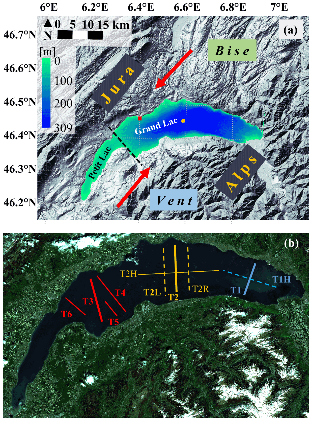
Figure 1 (a) Lake Geneva and surrounding topography, adapted from a public domain satellite image (https://worldwind.arc.nasa.gov/, last access: 29 October 2022) and bathymetry data from https://www.swisstopo.admin.ch/ (last access: 29 October 2022). The colour bar indicates the water depth. SHL2 (yellow cross) is a long-term CIPEL monitoring station where data on physical and biological parameters are measured. The red square shows the location of the EPFL Buchillon meteorological station (100 m offshore). The dashed black line approximately delimits the two basins of Lake Geneva called the Petit Lac (west) and the Grand Lac (east). The thick red arrows indicate the direction of the two strong dominant winds, called the Bise (coming from the north-east) and the Vent (coming from the south-west). (b) A schematic view of transects (T) selected for the different field campaigns in this study (for details, see text and Table S1 in the Supplement). The background satellite image is taken from Sentinel-1A.

2.2 Hydrodynamic modelling

In this study, MITgcm (Marshall et al., 1997), which solves the 3D Boussinesq, hydrostatic Navier–Stokes equations (including the Coriolis force), was used in a series of numerical simulations for Lake Geneva for 2018 and 2019, based on the validated model set-up of Cimatoribus et al. (2018). The model was forced by meteorological data (wind fields, atmospheric temperature, humidity, solar radiation) extracted from the COnsortium for Small-scale MOdeling (COSMO) atmospheric model (http://www.cosmo-model.org/content/tasks/operational/default.htm (last access: 5 December 2022; Voudouri et al., 2017). COSMO data are also used in the EOF analysis. The first modelling step was a low-resolution (LR) model (horizontal resolution of 173 to 260 m, 35 depth layers, integration time step of 20 s), which was initialized from rest using the temperature profile from CIPEL station SHL2 (CIPEL, 2019) measured on 25 October 2017 and 19 December 2018, respectively (calm weather conditions prevailed on both dates). For each run, the LR model spin-up was ∼180 d. The 3D interpolated results of the LR modelling were then used to initialize the high-resolution (HR) version of the model (horizontal resolution of 113 m and 50 depth layers, with layer thicknesses ranging from 0.30 m at the surface to approximately 12 m for the deepest layer and integration time step of 6 s). For each year, the HR model was run for two seasons: under weakly stratified conditions (November–April) and under strongly stratified conditions (May–October).

The model's capability to realistically reproduce stratification, mean flow, and internal seiche variability in Lake Geneva was demonstrated by Cimatoribus et al. (2018, 2019). To further assess the model's ability to reproduce seasonal stratification, a separate validation was carried out in the present study using temperature profiles measured in 2019 at SHL2 (Fig. S1 in the Supplement), located at the centre of the Grand Lac (Fig. 1a).

2.3 Transect field measurements

Based on the proposed procedure, six transects were selected in different parts of the Grand Lac (Fig. 1b), i.e. one transect in the eastern part and five in the central and western parts (details below). The large-scale gyre in the central part of the Grand Lac was the main focus of the transect field measurements due to its importance and persistence. Along each transect, 10 profiles of current velocity spaced 1 km apart were measured, each for at least 5–10 min using an acoustic Doppler current profiler (ADCP; Teledyne Marine Workhorse Sentinel) with the transducer located at 0.5 m depth. The ADCP was equipped with a bottom-tracking module, set up for one hundred 1 m bins (blanking distance of 2 m), and operated in high-resolution processing mode. Tilt and heading angles were derived from sensors located inside the instrument. Vertical profiles of water temperature were measured with a Sea and Sun Marine Tech CTD75M multi-parameter probe at predefined points during the field campaigns. The conductivity–temperature–depth (CTD) probe was lowered at a speed of ∼10 cm s⁻¹. It recorded data at 7 Hz, thus providing a sampling resolution of ∼1.5 cm.

2.4 SAR remote sensing

Synthetic aperture radar (SAR) is frequently used to detect oceanic surface features under light wind conditions (Johannessen et al., 1996; Wang et al., 2019). The main advantages of SAR imagery are that (i) it functions day and night under all weather conditions, (ii) it has high sensitivity to small-scale variability in the water surface, and (iii) it provides high-resolution images. The patterns observed in SAR images are due to the change in water surface roughness, which is influenced by wave–current interactions, natural surface films, and spatial variations in the local wind field (Johannessen et al., 2005). Gyres or eddies in SAR images are indicated by dark spiral features called “black” or “classical” eddies (Karimova, 2012; Hamze-Ziabari et al., 2022a). More details are given in Sect. S1. For the present study, C-band SAR data were obtained from the European Space Agency's (ESA) Sentinel-1A and Sentinel-1B satellites. The co-polarized VV (vertical transmit, vertical receive SAR polarization) data were used because noise restricts the application of VH (vertical transmit, horizontal receive SAR polarization) data (Gao et al., 2019). The spatial resolution of SAR data varies between 5 and 20 m for a ground sampling distance of 10 m.

2.5 Okubo–Weiss parameter and empirical orthogonal functions

The Okubo–Weiss (OW) parameter describes the local strain–vorticity balance in the horizontal flow field of a shallow fluid layer. It allows separation of vorticity-dominated regions associated with basin-scale gyres or mesoscale eddies from strain-dominated ambient regions (Okubo, 1970; Weiss, 1991) and can be written as

$$\begin{array}{}\text{(1)}& \mathrm{OW}=S_{\mathrm{n}}^{\mathrm{2}}+S_{\mathrm{s}}^{\mathrm{2}}-{\mathit{\omega }}_z^{\mathrm{2}},\end{array}$$

where S_n is the normal component of strain, S_s is the shear component of strain, and ω_z is the relative vorticity of the flow, defined by, respectively,

$$\begin{array}{}\text{(2)}& {\displaystyle }{S}_{\mathrm{n}}={\displaystyle \frac{\partial u}{\partial x}}-{\displaystyle \frac{\partial v}{\partial y}}\text{(3)}& {\displaystyle }{S}_{\mathrm{s}}={\displaystyle \frac{\partial v}{\partial x}}+{\displaystyle \frac{\partial u}{\partial y}}\text{(4)}& {\displaystyle }{\mathit{\omega }}_z={\displaystyle \frac{\partial v}{\partial x}}-{\displaystyle \frac{\partial u}{\partial y}},\end{array}$$

where u and v are Cartesian components of the horizontal flow field. Positive OW values relate to strain-dominated regions, whereas negative OW values identify vorticity-dominated regions.

For a given data set, EOF analysis identifies the main spatial patterns (E) and their temporal evolution (P) (Wang and An, 2005). Hourly averaged OW values derived from numerical simulations were decomposed into the basis function $E_{\mathrm{OW}}^k\left(X\right)$ and the principal component coefficient $P_{\mathrm{OW}}^k\left(t\right)$ as

$$\begin{array}{}\text{(5)}& \mathrm{OW}\left(X,t\right)={\sum }_{k=\mathrm{1}}^N{E}_{\mathrm{OW}}^k\left(X\right)P_{\mathrm{OW}}^k\left(t\right),\end{array}$$

where k is the EOF mode, which varies from 1 to the maximum N, X= (x, y) is the position under consideration, and t is time. The $E_{\mathrm{OW}}^k\left(X\right)$ modes identify the spatial patterns of the OW parameter. The time evolution of each $E_{\mathrm{OW}}^k\left(X\right)$ mode can be obtained from the time series of principal component coefficients, indicated as $P_{\mathrm{OW}}^k\left(t\right)$.

3 Procedure for detecting gyres

The proposed gyre identification procedure consists of four steps (Fig. 2): (i) data pre-processing, (ii) extracting dominant patterns using EOF analysis of OW fields, (iii) defining the 3D structure of the gyre, and (iv) finding the correlation between the dominant gyre pattern and environmental forcing.

In step (i), the OW values are computed for selected time windows using the horizontal velocity fields (u, v) generated by the 3D numerical modelling. Vorticity-dominated and strain-dominated regions can be identified from OW values and can then, in step (ii), be used to locate and characterize the gyre flow field, in particular gyre centres and the outer limits of gyres, located where vorticity and strain are approximately in balance. This is further supported and confirmed by patterns detected in SAR images. This OW and EOF analysis is repeated for several depths in step (iii) to verify that this surface pattern documents a gyre extending over the upper layers, with its depth limited by the thermocline. Step (iv) links the observed dominant OW pattern to the forcing that generated it, thereby identifying forcing patterns, mainly wind events, preceding the formation of gyre patterns. Scrutinizing actual meteorological data for such forcing patterns will then allow planning of when and where to take detailed transect field measurements of the gyre pattern in the lake.

3.1 Detection of the core of a gyre or eddy

The separation of the OW field in terms of its sign can be used to detect cores of complex fluid flows (McWilliams, 1984; Elhmaïdi et al., 1993). These cores are characterized by negative OW values below a given (negative) threshold, OW_T (Pasquero et al., 2001; Isern-Fontanet et al., 2006; Henson and Thomas, 2008; Liu et al., 2021). For this purpose, a threshold value of OW_T=0.2σ_ow was defined, where σ_ow is the root-mean-square fluctuation in OW in the epilimnion with the same sign of the vorticity of the gyre/eddy core (Pasquero et al., 2001; Isern-Fontanet et al., 2006; Henson and Thomas, 2008).

In the data pre-processing stage, the hourly computed OW values were normalized by hourly values of OW_T such that the normalized OW parameter, OW_N, partitions the topology of the gyre/eddy field into three regions: elliptic regions, OW${}_{\mathrm{N}}<-\mathrm{1}$; hyperbolic regions, OW_N>1; and a background field, $\left|{\mathrm{OW}}_{\mathrm{N}}\right|\le \mathrm{1}$ (Pasquero et al., 2001; Isern-Fontanet et al., 2006). As shown in Fig. 2, elliptic regions, which represent the centre of gyres/eddies, are significantly more pronounced than the other regions. In lakes, basin-scale gyres are mainly restricted by the lake basin geometry and also impacted by the surrounding topography. Therefore, the regions with OW${}_{\mathrm{N}}>-\mathrm{1}$ can be influenced by the interaction between gyres and nearshore boundaries. As a result, a wide spatial variability in OW_N values in these regions was observed, whereas regions with OW${}_{\mathrm{N}}<-\mathrm{1}$ were spatially rather stable. To eliminate such variability from the spatial and temporal identification of gyres/eddies, regions with OW${}_{\mathrm{N}}>-\mathrm{1}$ were filtered out before implementing the EOF analysis.

For the proposed procedure (Fig. 2), hourly filtered OW_N values of different depth layers were computed for each month. The EOF analysis was then applied to detect the main modes (spatial pattern) and the corresponding principal component time series. From different modes of the EOF results, signatures of gyre or eddy cores were identified based on the following criteria:

1. A local extreme value exists in the spatial modes of the OW_N values.

2. At least one closed line exists around each local extreme value.

3. The core edge is identified as the closed line where the sign of $E_{{\mathrm{OW}}_{\mathrm{N}}}{P}_{{\mathrm{OW}}_{\mathrm{N}}}$ changes.

4. A vertical and horizontal coherence of a gyre or eddy signature must exist between different depth layers (bounded below by the thermocline); i.e. criteria 1–3 above must be spatially consistent for different depth layers.

By applying these criteria, the location of gyre and eddy centres can be identified.

3.2 Detecting the outer boundary of a gyre or an eddy

Gyre boundaries are located where vorticity and strain are approximately in balance, i.e. $\left|{\mathrm{OW}}_{\mathrm{N}}\right|\le \mathrm{1}$. However, as discussed above, the outer gyre boundaries cannot be completely resolved by the OW analysis. Furthermore, the noise in the resulting OW_N fields makes the detection of coherent flow structures difficult (Souza et al., 2011). Defining vertical- and horizontal-coherence criteria that can confirm coherent 3D gyre patterns can significantly reduce this limitation of the OW analysis. This threshold-based boundary detection method can be complemented by a geometry-based method using contour lines in synthetic aperture radar (SAR) images. Therefore, information about the outer boundaries in support of the OW_N analysis results can be obtained from SAR imagery, since basin-scale gyres and large eddies can be detected in SAR images.

3.3 Finding the link between the temporal variation in a gyre and environmental forcing

Wind stress and surface buoyancy flux (due to heating and cooling) are the processes controlling gyre circulations and their variability. To find a link between the pattern of external forcing and the computed spatial pattern of the OW_N parameter presented in the previous sections, monthly EOF analyses of the total wind stress ($\sqrt{{\mathit{\tau }}_x^{\mathrm{2}}+{\mathit{\tau }}_y^{\mathrm{2}}}$) and the net upward heat flux extracted from the COSMO atmospheric data are implemented. In the final stage of the procedure, the lagged cross-correlations between the spatial mode and the corresponding principal component time series of the environment forcing and the OW_N are examined.

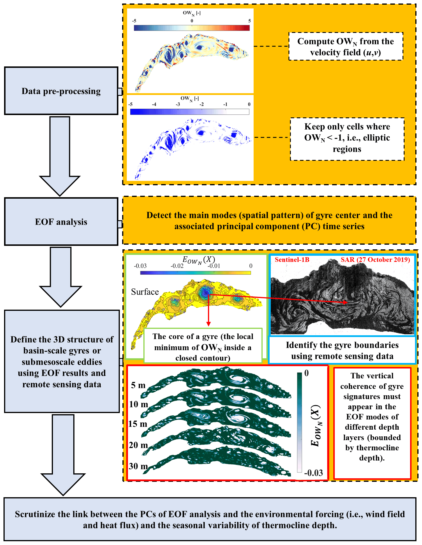
Figure 2 Flowchart of the proposed procedure showing the four steps (grey boxes) for detecting basin-scale gyres and eddies applied to Lake Geneva. Modelling results for the October 2019 Bise wind event, together with the corresponding SAR image, are used to highlight certain steps of the proposed procedure. For details, see text.

4 Results

In this section, the performance of the procedure for detecting the temporal and spatial variations in gyres/eddies is first evaluated for September 2018. Thereafter, the robustness of the proposed procedure is assessed by comparing results based on transect measurements from several transect field campaigns that were carried out based on the proposed procedure between September, when the lake is strongly stratified at a shallow depth, and December, when it is weakly stratified at a greater depth.

4.1 Detecting gyres and eddies: Okubo–Weiss parameter and EOF analysis

4.1.1 Detection of gyre centre locations

Results of 3D modelling for September 2018 are used to demonstrate the performance of the proposed procedure. The first and second modes of the OW_N variations in different depth layers (1, 5, 10, 15, 20, and 30 m) are given in Fig. 3a and b. Due to the quick convergence of the EOF decomposition modes, only the first two dominant EOF modes are analysed for detecting elliptic regions with negative OW_N values. The first mode dominates the overall OW_N variations. It accounts for nearly 56 % of the total variance in the layers down to 15 m depth and ∼47 % for deeper depths. The second mode contributes nearly 23 % to the total variance for the near-surface layers. Down to 30 m depth, each of the remaining modes contains less than 5 % of the total variance (not shown).

Three closed trajectories that encircle regions with negative $E_{{\mathrm{OW}}_{\mathrm{N}}}$ values can be distinguished in the first mode at different depth layers (Fig. 3a). These regions indicate the presence of three large-scale gyres in the Grand Lac, if $E_{{\mathrm{OW}}_{\mathrm{N}}}{P}_{{\mathrm{OW}}_{\mathrm{N}}}<\mathrm{0}$ (the time series of $P_{{\mathrm{OW}}_{\mathrm{N}}}$ is discussed in the following sections). For better visualization, only negative values associated with $E_{{\mathrm{OW}}_{\mathrm{N}}}$, which document gyre patterns according to the definition in Sect. 3.1, are presented. Positive values of $E_{{\mathrm{OW}}_{\mathrm{N}}}$ are shown in Fig. S2. The location of the centre of each gyre in different depth layers is calculated by averaging the coordinates of the gyre centres (based on criteria 1–3 presented above). The closed trajectories weaken with depth down to 20 m and disappear at 30 m depth due to the presence of the thermocline, which is situated at ∼15 m depth. A region bounded by closed trajectories with negative OW_N values can also be considered to be an indicator for areas where pelagic upwelling or downwelling is more likely to occur. Details of the spatial OW_N pattern (e.g. Fig. 4b, d) confirm the presence of negative OW_N regions in the centre of the large-scale gyres. The rotation sign of the three-gyre pattern after the Bise event is given in Figs. S3–S5 for different months. The anticyclonic gyre (clockwise rotating) in the west and two cyclonic gyres (anticlockwise rotating) in the centre and in the east of the Grand Lac are hereinafter referred to as AG, CG1 and CG2, respectively (Fig. 3a). The second EOF mode reveals the simultaneous existence of smaller eddies, often with shorter lifetimes than basin-scale gyres (Fig. 3b). More details on these eddies are presented below.

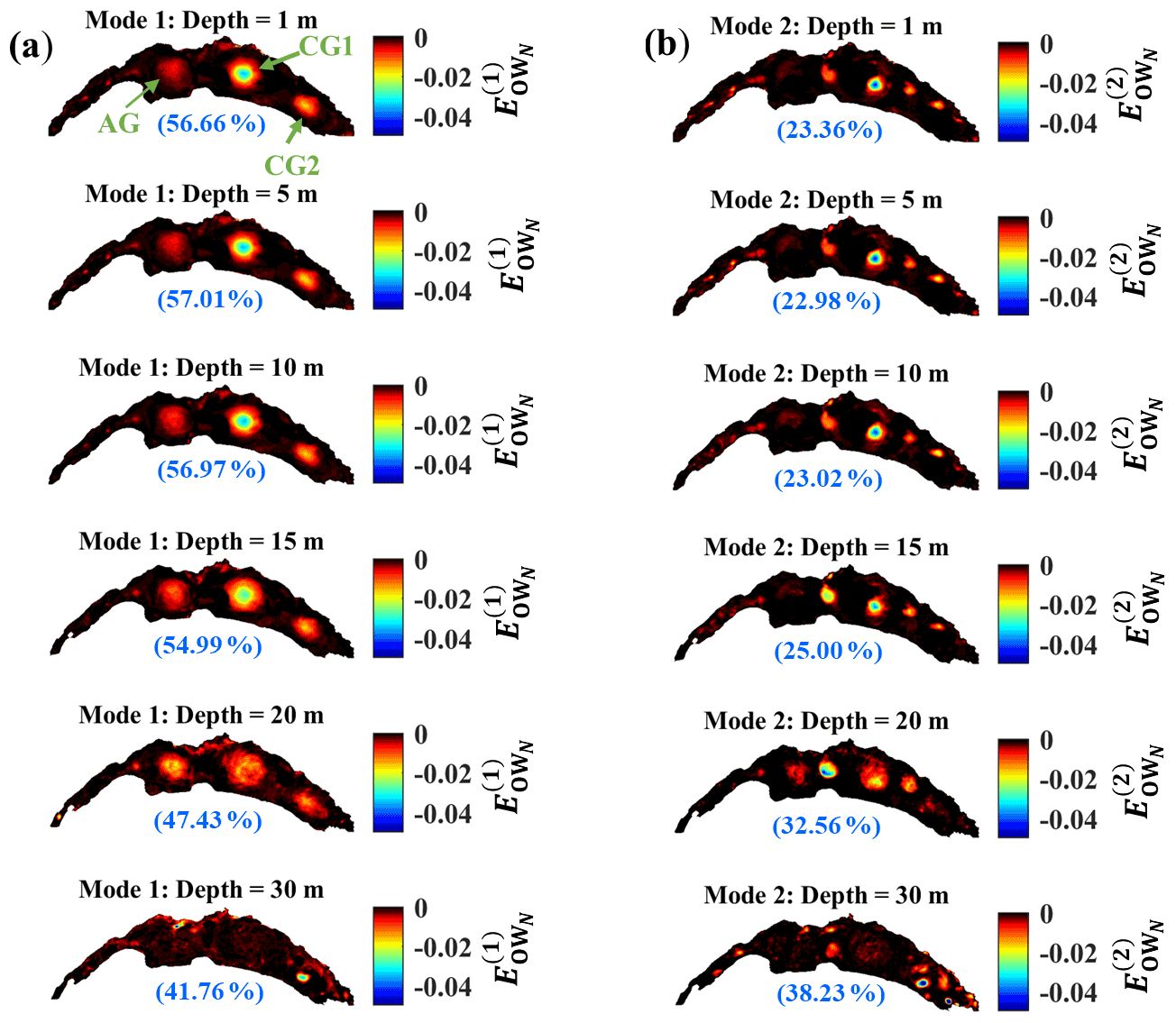
Figure 3 EOF analysis of the MITgcm output for Lake Geneva for the month of September 2018: (a) first mode (left column) and (b) second mode (right column) of the EOF of OW_N are shown for different depth layers. The first mode is dominated by three large-scale gyres (circular zones of negative $E_{{\mathrm{OW}}_{\mathrm{N}}}$ values), whereas in the second mode, (sub)mesoscale eddies also appear. The contributions to the total variance of the monthly OW_N values are given by the percentage indicated (in blue) for each layer and each mode. Colour bars give the range of the EOF.

4.1.2 Detection of the outer boundary of a gyre or an eddy

The OW_N analysis shows that gyre centres have strongly negative OW_N values and that positive OW_N areas surround the gyres (Fig. 4b, d). The transition zone between the two zones ($\left|{\mathrm{OW}}_{\mathrm{N}}\right|\le \mathrm{1}$), which should indicate the outer edge of the gyre, is wide in certain parts of the circumference and does not allow determination of the outer edge of the gyre (Fig. 4b, d). SAR images may be used to confirm/define this edge (more details in Sect. S1 in the Supplement). The boundaries between the two cyclonic gyres, CG1 and CG2, located in the eastern part of lake, can be determined from SAR data obtained from Sentinel-1 on 21 July and 12 October 2018 (Fig. 4a, c), where two (elliptical) gyres are evident. The minor (major) axes of CG1 and CG2 are approximately 6.5 (12.9) and 9.8 km (15.9 km), respectively. Smaller eddies, marked by strong negative OW_N values in their centre, surround the large-scale CG1 and CG2 gyres.

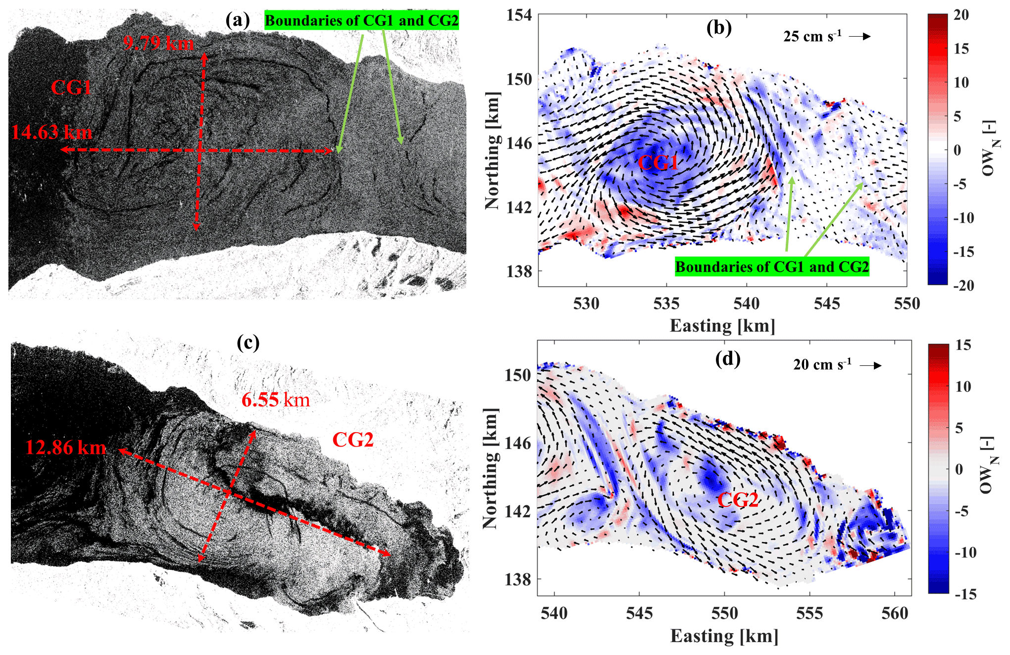
Figure 4 (a, c) SAR images (Sentinel-1) indicating two cyclonic gyres (CGs) in the eastern part of Lake Geneva for (a) CG1 (21 July 2018) and (c) CG2 (12 October 2018). Dashed red lines: major gyre axes and their dimensions. (b, d) Corresponding modelled surface velocity fields (small black arrows) and OW_N parameter values (colours). Strong negative OW_N parameter values (blue) indicate the location of core zones of large-scale gyres and mesoscale eddies. The colour bars give the range of the OW_N values.

4.1.3 Detecting large-scale gyres: link between environmental forcing and gyre signature

To find a link between the pattern of external forcing and the computed spatial pattern of OW_N, EOF analyses of the total wind stress and the net upward heat flux extracted from the COSMO atmospheric data for September 2018 were carried out. The first spatial mode and the corresponding principal component time series of the total wind stress ($c_{\mathrm{w}}^{\left(\mathrm{1}\right)}\left(x{)}_{,}{\mathit{\phi }}_{\mathrm{w}}^{\left(\mathrm{1}\right)}\right(t\left)\right)$ and the upward heat flux ($c_{\mathrm{HF}}^{\left(\mathrm{1}\right)}\left(t\right)$, ${\mathit{\phi }}_{\mathrm{HF}}^{\left(\mathrm{1}\right)}\left(t\right))$ are presented in Fig. 5a and b, respectively. The first mode of the external forces dominates the variation in the forces, since it constitutes ∼98 % and 99 % of the total variance related to the total wind stress and heat flux, respectively. The total variance differences between the first spatial modes and the principal component time series obtained from the solution with two dominant modes and the solution with all possible modes are negligible (O(10⁻¹⁰–10⁻¹⁴)) compared to the calculated absolute values (O(10⁻³)) (Fig. S6).

The EPFL Buchillon field station (Fig. 1b) data show that a strong Bise event started at ∼00:00 CET on 24 September 2018 and ended at ∼11:00 CET on 26 September 2018. The mean wind speed ±1 standard deviation was 4.21±1.88 m s⁻¹ with wind gusts of 8.40±3.37 m s⁻¹. The mean wind direction was 61±13^∘(Fig. 5e, f). Note that Buchillon field station data are only presented here to demonstrate that the EOF results shown in Fig. 5a and b represent realistic wind fields; they are not used in the EOF analyses. Average wind speed and direction over the whole lake surface extracted from COSMO during the Bise event that lasted from 24 to 26 September 2018 are given in Fig. S7. Figure 5e suggests that there is a link between the strong Bise event and the first EOF mode of OW_N indicated by the principal component ($P_{{\mathrm{OW}}_{\mathrm{N}}}^{\left(\mathrm{1}\right)}\left(t\right))$ time series. To determine this link, lagged cross-correlations were computed between the principal component time series of the dominant EOF modes of atmospheric forcing, i.e. the total wind stress (${\mathit{\phi }}_{\mathrm{w}}^{\left(\mathrm{1}\right)}\left(t\right))$ and the net upward heat flux, (${\mathit{\phi }}_{\mathrm{HF}}^{\left(\mathrm{1}\right)}\left(t\right))$, and the two dominant EOF modes of OW_N (Fig. 6). The lagged cross-correlation between the upward heat flux and $P_{{\mathrm{OW}}_{\mathrm{N}}}^{\left(\mathrm{1}\right)}\left(t\right)$ does not exceed 0.3 in the depth layers influenced by the gyres (2–20 m; Fig. 3). On the other hand, the cross-correlation between ${\mathit{\phi }}_{\mathrm{w}}^{\left(\mathrm{1}\right)}\left(t\right)$ and $P_{{\mathrm{OW}}_{\mathrm{N}}}^{\left(\mathrm{1}\right)}$ reaches values >0.8 in the same depth layers and a positive peak with a lag of 1–1.5 d for the near-surface layers (1–20 m; Fig. 6a–f). A positive peak means that ${\mathit{\phi }}_{\mathrm{w}}^{\left(\mathrm{1}\right)}\left(t\right)$ and $P_{{\mathrm{OW}}_{\mathrm{N}}}^{\left(\mathrm{1}\right)}\left(t\right)$ have the same sign. These results imply that the three-gyre pattern in the first mode (Fig. 3a) is predominantly controlled by the spatial $c_{\mathrm{w}}^{\left(\mathrm{1}\right)}\left(x\right)$ and temporal ${\mathit{\phi }}_{\mathrm{w}}^{\left(\mathrm{1}\right)}\left(t\right)$ variations in wind stress. Furthermore, the time series of the first mode, $P_{{\mathrm{OW}}_{\mathrm{N}}}^{\left(\mathrm{1}\right)}\left(t\right)$, in different depth layers suggest that the three-gyre pattern can persist for nearly 5 d after the wind peak (Fig. 5e).

Thereafter (29 September 2018), the large-scale gyres break down into smaller gyres/eddies, and the second OW_N mode dominates (Fig. 5f). The cross-correlation between wind stress, upward heat flux, and $P_{{\mathrm{OW}}_{\mathrm{N}}}^{\left(\mathrm{2}\right)}\left(t\right)$ is not greater than 0.35 in the depth layers influenced by the gyres (Fig. 6g–l). For wind stress, $E_{{\mathrm{OW}}_{\mathrm{N}}}^{\left(\mathrm{2}\right)}$ is excited with a lag of ∼5.5 d, with the same sign, and for upward heat flux with a lag of more than 4 d, again with the same sign. Moreover, negative peaks in the cross-correlation between $E_{{\mathrm{OW}}_{\mathrm{N}}}^{\left(\mathrm{2}\right)}$ and ${\mathit{\phi }}_{\mathrm{HF}}^{\left(\mathrm{1}\right)}\left(t\right)$ show that $E_{{\mathrm{OW}}_{\mathrm{N}}}^{\left(\mathrm{2}\right)}$ can be excited with a lag of 1–2 d due to differential heating and cooling during day–night cycles (Fig. 6g–l). However, $E_{{\mathrm{OW}}_{\mathrm{N}}}^{\left(\mathrm{2}\right)}$ is only weakly excited by wind stress or upward heat flux. In addition to the effects of environmental forcing presented above, the basin shape and bathymetry also change the gyre pattern over time.

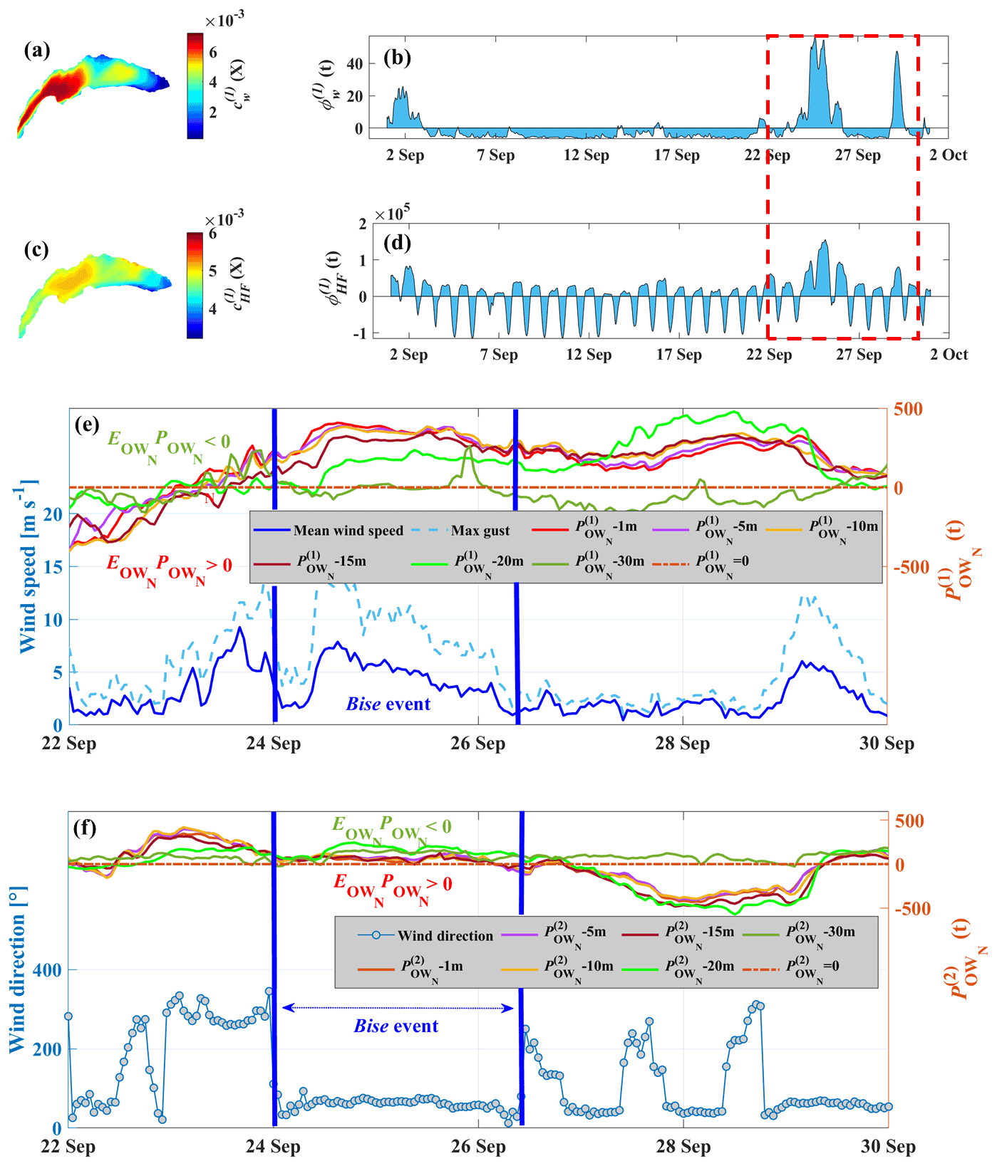
Figure 5 For September 2018: (a) first spatial mode ($c_{\mathrm{w}}^{\left(\mathrm{1}\right)}\left(X\right))$ and (b) principal component time series (${\mathit{\phi }}_{\mathrm{w}}^{\left(\mathrm{1}\right)}\left(t\right))$ of the total wind stress. (c) First spatial mode $c_{\mathrm{HF}}^{\left(\mathrm{1}\right)}\left(X\right)$ and (d) principal component time series (${\mathit{\phi }}_{\mathrm{HF}}^{\left(\mathrm{1}\right)}\left(t\right))$ of the net upward heat flux. (e) Top: principal component time series of OW_N associated with the first spatial mode ($P_{{\mathrm{OW}}_{\mathrm{N}}}^{\left(\mathrm{1}\right)}\left(t\right))$ in different depth layers. Bottom: mean wind speed and wind gusts at the Buchillon station (see Fig. 1 for location) for the period indicated by the dashed-red-lined box in (b) and (d). (f) Top: the principal component time series of the OW_N parameter associated with the second spatial mode ($P_{{\mathrm{OW}}_{\mathrm{N}}}^{\left(\mathrm{2}\right)}\left(t\right))$ at different depth layers. Bottom: wind direction at the Buchillon station for the period indicated by the dashed-red-lined box in (b) and (d). Colour bars in (a) and (c) show the range of the parameters. The colours in the legends of (e) and (f) correspond to the different depths. In (e) and (f), negative $E_{{\mathrm{OW}}_{\mathrm{N}}}{P}_{{\mathrm{OW}}_{\mathrm{N}}}$ indicates the negative OW_N values (the elliptic regions) that are characteristic of gyres. Note that all EOF analyses are based on COSMO meteo data. The two vertical blue lines mark the duration of the Bise wind event.

Figure 6 (a–f) Lagged cross-correlation of the principal component time series of the total wind stress (${\mathit{\phi }}_{\mathrm{w}}^{\left(\mathrm{1}\right)}\left(t\right))$ and the net upward heat flux (${\mathit{\phi }}_{\mathrm{HF}}^{\left(\mathrm{1}\right)}\left(t\right))$ with the principal component time series of the OW_N parameter associated with the first spatial mode ($P_{{\mathrm{OW}}_{\mathrm{N}}}^{\left(\mathrm{1}\right)}\left(t\right))$ in different depth layers. (g–l) Lagged cross-correlation of the principal component time series of the total wind stress (${\mathit{\phi }}_{\mathrm{w}}^{\left(\mathrm{1}\right)}\left(t\right))$ and the net upward heat flux (${\mathit{\phi }}_{\mathrm{HF}}^{\left(\mathrm{1}\right)}\left(t\right))$ with the principal component time series of the OW_N parameter associated with the second spatial mode ($P_{{\mathrm{OW}}_{\mathrm{N}}}^{\left(\mathrm{2}\right)}\left(t\right))$ in different depth layers. Wind stress and heat flux are defined in the colour legend in panel (a).

4.2 Detecting large-scale gyres: transect field campaigns

4.2.1 A cyclonic gyre at the centre of the Grand Lac

To validate the proposed procedure for detecting the location and time of basin-scale gyres after a strong wind event, a field measurement campaign was performed in September 2019. This campaign focused on capturing the largest basin-scale gyre, CG1, in the central part of the Grand Lac (Figs. 3, 4). Buchillon field data recorded a strong Bise event that started on 17 September 2019 at ∼20:00 CET and ended on 20 September 2019 at ∼13:00 CET (mean wind speed ±1 standard deviation was 3.65±0.86 m s⁻¹, with gusts of 7.69±1.78 m s⁻¹ and mean wind direction of $\mathrm{64}\pm \mathrm{11}{}^{\circ }$). Furthermore, the spatial pattern of averaged wind speed and direction computed from the forecasted COSMO atmospheric data (Fig. 7a) revealed the same spatial pattern as had been observed for the September 2018 Bise event (Fig. S7) discussed above. For September 2018, it was shown that the three-gyre system pattern is highly correlated with strong Bise events (Figs. 5, 6). This pattern forms and persists for several days after the wind event has ceased. Therefore, based on these results, a field campaign was designed to capture the boundary and temporal variation in CG1 from 20 to 22 September 2019.

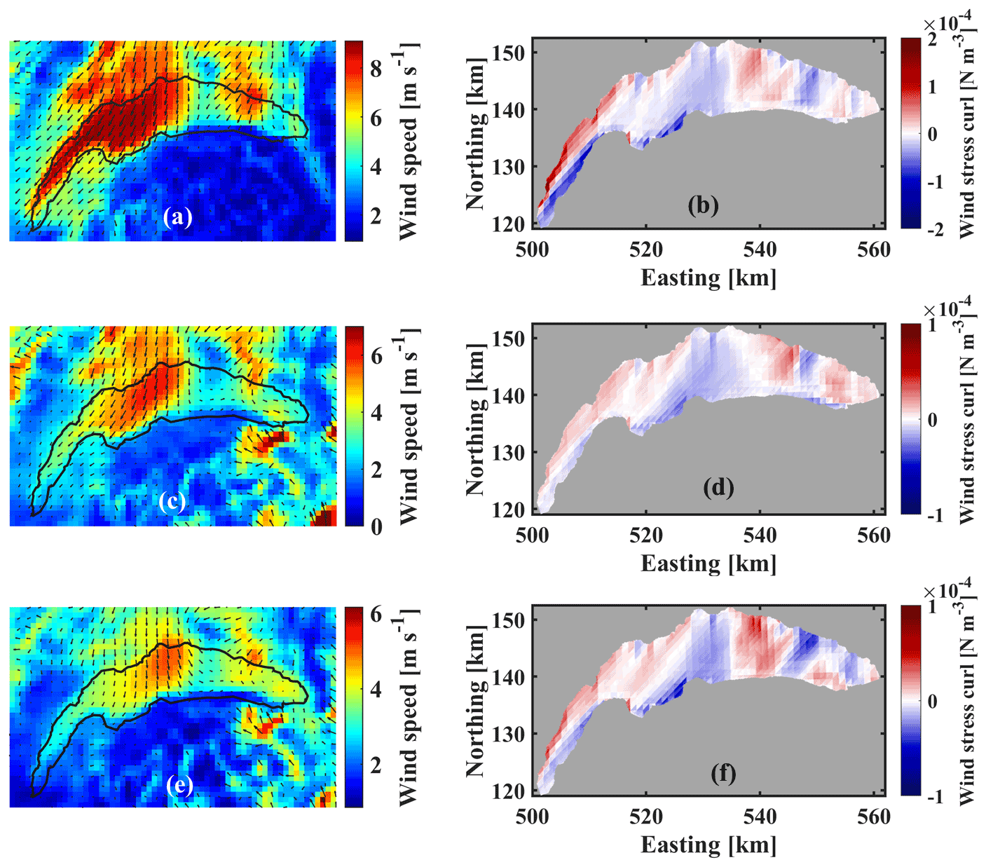
Figure 7 (a, c, e) Averaged wind speed and direction extracted from COSMO data for Bise events. (b, d, f) The computed wind stress curl during the corresponding Bise events. Panels (a) and (b) from 17 to 20 September 2019, (c) and (d) from 21 to 23 October 2019, (e) and (f) from 18 to 23 November 2019. Colour bars indicate the range of parameters.

Four transects, T2, T2L, T2R, and T2H (Fig. 1b; coordinates are given in Table S1), were chosen to investigate the 3D structure of CG1 and its evolution. A few hours after the strong Bise event ended on 20 September, measurements at 10 points with 1 km spacing along transect T2, from south to north, were taken. The duration of field measurements along the vertical (T2, T2L, T2R) and horizontal (T2H) transects was 2 to 3 h each. More details are given in Table S1. The measured velocity field confirmed the existence of a cyclonic circulation in the centre of the Grand Lac (Fig. 8a, b). In the proposed procedure, the centre of each gyre is calculated by averaging the coordinates of the centres of the minimum OW_N zones in different depth layers. To take into account the uncertainty in selecting the location of each transect, the standard deviation of the coordinates of the minimum OW_N zones from the average transect was also calculated. It was ∼1.8 km for September 2018. This uncertainty was considered by taking measurements along two additional transects, T2R and T2L, that covered the low-velocity core zones (almost zero) surrounding the centre. The velocity field for each transect is given in Fig. 8c. The 3D velocity field shows a cyclonic gyre. The gyre velocity field penetrated down to ∼15 m, limited by the strong thermal stratification in September (see Fig. S1 for temperature profile at SHL2 near the centre of CG1). The maximum horizontal water velocity reaches ∼35 cm s⁻¹ in the near-surface layer. The centre of the cyclonic gyre can clearly be seen in all transects by the strong decrease in horizontal velocity.

In order to capture the gyre boundary and to determine the complete CG1 velocity field, 12 points with 1.5 km spacing were measured along transect T2H (see Fig. 1b for location), from west to east, on 22 September. For example, point 1 at the western end of the transect was clearly outside the gyre field because both the velocity magnitude and direction changed. Transect 2 (T2), from south to north, was repeated. The field results (Fig. 8d) confirmed the boundaries of CG1, which were identified in the SAR image (see Fig. 4a). Furthermore, the velocity field shows that the nearshore (south and north) currents are much stronger than currents at the east and west boundaries of CG1, indicating that the nearshore bathymetry deforms/confines the gyre flow field.

An analysis similar to that of September 2018 discussed above was carried out for September 2019, with similar results (Fig. S8). Comparisons between the modelled and observed velocity fields for the September 2019 campaign are given in Fig. S3, again confirming the good agreement between the field observations and the results of the numerical modelling.

Figure 8 Measured current velocity field for sampling points along the selected transects (T) shown in Fig. 1b for (a) current vector profiles and (b) contour plot for 20 September 2019, (c) vectors (black arrows) and contours (see colour bar legend) for 21 September 2019, (d) current vector profiles, (e, f) contour plots for 22 September 2019. The coordinates of sampling points in T2 are the same in (a)–(d) and (f). The colour bars indicate horizontal velocity in centimetres per second. Positive velocities are pointing eastward for transect T2 and northward for transect T2H. Colour bars give the range of the horizontal velocity.

4.2.2 Observations of two- and three-gyre patterns

In most previous numerical studies on Lake Geneva, two basin-scale gyres (a dipole), located in the centre of the deep Grand Lac basin, were considered to be the main basin-scale circulation (Le Thi et al., 2012; Razmi et al., 2017), although the EOF analysis predicted three large-scale gyres (Figs. 3, 4). To confirm the existence of a dipole in Lake Geneva, field measurements were conducted from 23 to 25 October 2019 and from 24 to 26 November 2019 after strong Bise wind events (Fig. S9). However, the primary objective of the field campaign on 25 October and 25 November 2019 was to determine whether three large-scale gyres predicted by the EOF analysis (Figs. 3, 4) exist in Lake Geneva.

The average wind direction during the Bise event in October 2019 was $\sim \mathrm{69}{}^{\circ }$ with a duration of 40 h (Fig. 7b) and was $\sim \mathrm{47}{}^{\circ }$ with a duration of 94 h in November 2019 (Figs. 7c, S9). For the October 2019 campaign, two transects, T2 (western part) and T3 (eastern part) (Fig. 1b), which consisted of 10 measurement points with 1 km spacing, were selected following the proposed procedure, but with different transect coordinates for each month. The duration of field measurements along transects T2 and T3 was ∼2 h each. To confirm the existence of the third gyre in the eastern part of the lake, CG2, two transects were selected, T1 and T1H (see Fig. 1b), each with eight points. The distance between the T1H measurement points was 1.5 km in order to capture the CG2 boundary observed in the SAR image (Fig. 4). The duration of the field measurements along transects T1 and T1H was ∼1.5 and 2.5 h, respectively. In the 3D velocity field recorded along different transects during the October campaign (Fig. 9a), a dipole consisting of an anticyclonic gyre, AG, at transect T3 and a cyclonic gyre, CG1, at T2 is clearly evident. The maximum velocity at CG1 (22 cm s⁻¹) is stronger than at AG (15 cm s⁻¹), with the velocity field of AG penetrating into deeper layers. The 3D velocity field observed at T1 and T1H confirms the existence of the third cyclonic gyre (CG2) in the eastern part of Lake Geneva (Fig. 10). The CG2 velocity field penetrated down to nearly 20 m, and the maximum horizontal water velocity reached ∼17 cm s⁻¹ near the surface layer. The depth of the CG2 gyre is similar to that of CG1, and the magnitude of its velocity is comparable to AG.

To further confirm the existence of the three-gyre pattern in Lake Geneva during weakly stratified months, measurements along the three transects, T1, T2, and T3 (Fig. 1b), were carried out in November 2019, based on the EOF analysis for November 2018. During November, a different location for T3 was chosen because, compared to the October campaign, a different spatial pattern was observed in the EOF results (see Table S1 and Sect. S2). The transects T1 (eastern part), T2 (central part), and T3 (western part) were sampled on the same day, with 9, 10, and 8 points, respectively, each with a 1 km spacing. The duration of field measurements along transects T1, T2, and T3 was ∼2 h each. The measured 3D velocity fields reveal two cyclonic circulations at T1 and T2 and one anticyclonic circulation at T3 (Fig. 9d–g). In contrast to the October campaign, the magnitude and depth of the velocity field at CG2 and CG1 are comparable. Comparisons between the modelled and observed velocity fields for the October and November 2019 campaigns show good agreement (Figs. S4 and S5).

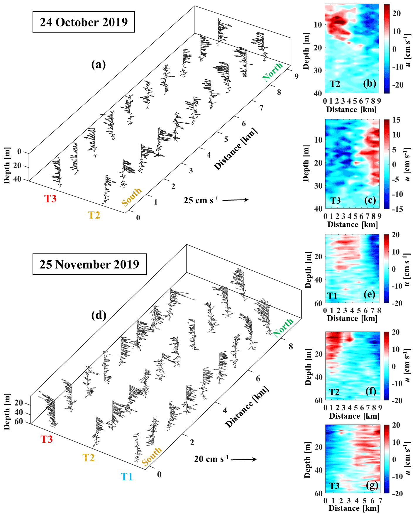
Figure 9 Field campaigns of October and November 2019 carried out along selected transects (T): (a) current velocity vector fields (arrows) of gyres AG (T3) and CG1 (T2) and (b, c) contour plots of the horizontal velocity, u, for 24 October 2019. (d) Current velocity vector field of gyres AG (T3), CG1 (T2), and CG2 (T1) and (e–g) contour plots of the horizontal velocity, u, for November 2019. The origin of the x axis is in the south. The colour bars indicate horizontal velocity in centimetres per second. Positive velocities are pointing eastward for transects T1, T2, and T3. For transect locations, see Fig. 1b.

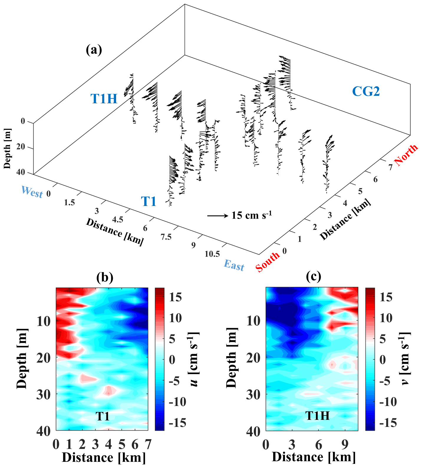
Figure 10 Field campaign of 25 October 2019: (a) current velocity field of CG2 shown as vector profiles at the different stations along transects T1 and T1H. (b, c) Contour plots of the horizontal components of velocity field, u (along T1) and v (along T1H). The origin of the x axis is in the south for T1 and in the west for TH1. The colour bars indicate horizontal velocity in centimetres per second. Positive velocities are pointing eastward for transects T1, T2, and T3 and northward for transect T1H. For transect location, see Fig. 1b.

4.3 Detecting small eddies

Small eddies have not yet been investigated in Lake Geneva. In the present study, smaller-sized coherent structures with negative OW_N values were detected in the vicinity of the basin-scale gyres or at coastal headlands (Fig. 3). Two dominant and frequently occurring patterns of such eddies were selected in the EOF analysis for different months (Figs. 11, 12). The focus here was on submesoscale eddies, SE1 and SE2 (see Fig. 11c for location), that have a lifetime of several days, comparable to the lifetime of basin-scale gyres. In the SAR images, small eddies appear as radar-dark filaments wound into spirals (Hamze-Ziabari et al., 2022a). A close similarity between the patterns observed in the SAR data and numerical results is observed (cf. Figs. 11 and 12). According to the numerical results, the rotation of SE1 is cyclonic, and its diameter was O(5) km during October 2019.

Such small-scale patterns cannot be adequately captured by velocity measurements at fixed points. Therefore, the ADCP was mounted on a small, boat-towed catamaran. Continuous vertical current profiles were measured along the preselected transects. SE1 was frequently observed by the proposed procedure during October 2018 and 2019 (not shown). A field campaign was conducted in October 2020 to investigate the vertical structure of SE1. Two transects, T4 and T5, were chosen based on EOF results and SAR images for 2018 and 2019. The horizontal lengths of T4 and T5 were ∼8.5 and 3.5 km, respectively. The spatial resolution of the measured current profiles depends on the boat's speed (1.5–2 km h⁻¹). The duration of field measurements along transects T4 and T5 was ∼5 and 2 h, respectively. Velocity data were averaged every minute, which resulted in a 25–33 m spatial resolution along each transect. The numerical results and measured horizontal velocities at T4 and T5 are given in Fig. 11e–h. A cyclonic circulation formed in the south-western part of the lake, and an anticyclonic circulation formed in the north-western part (Fig. 11d). There is a close match between the measured and modelled velocity fields (see Fig. 11e–h). Field data indicate that the velocity field of SE1 extended to depths between 35–40 m, comparable to the depth of the anticyclonic gyre (AG) in this part of the lake measured during the October 2019 campaign.

Flow separation in the vicinity of headlands or baroclinicity due to favourable upwelling in the Petit Lac can also lead to the formation of submesoscale eddies, such as SE2 (Fig. 12). The dimensions of SE2 are generally smaller than those of SE1. However, SE2 is more frequently observed during certain months of the year. For example, the signature of SE2 can be clearly observed in SAR images taken on 19 August and 7 November 2018 (Fig. 12). The numerical results confirm the presence of cold cyclonic eddies with the same dimensions for the same period (Fig. 12b, d). The lateral extent of SE2 is O(4 km). A field campaign on 3 September 2020 confirmed the existence of SE2. The simulated and measured velocity fields indicate a cyclonic circulation in the north-western part of the Grand Lac basin of Lake Geneva (Fig. 12e, f). Field data show that the SE2 velocity field can reach 20 m depth, which is 5 m deeper than the depth of the cyclonic circulation during the September 2019 campaign. Although it is beyond the scope of this study to investigate the origin of small eddies, it was demonstrated that the proposed procedure can detect and locate them correctly, as was confirmed by transect field measurements. Generally, such small eddies are expected to be transient in nature. However, eddies SE1 and SE2 were trapped between large-scale gyres or between lake basin boundaries and gyres. They hardly lost any strength and remained active at fixed locations for several days, comparable to the lifetime of large-scale gyres.

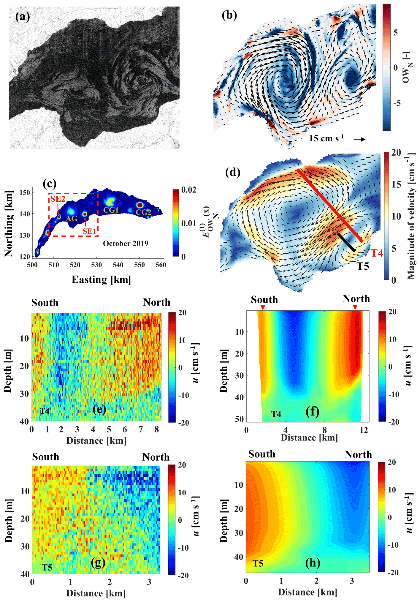
Figure 11 Evidence for the existence of submesoscale eddy 1 (SE1). (a) Remote sensing evidence (SAR images, Sentinel-1) of SE1 for 27 October 2019. (b) Corresponding modelled surface velocity fields (small black arrows show sense of rotation) and OW_N values shown by colours. (c) First EOF mode of OW_N for October 2019 showing large gyres AG1, CG1, and CG2 and small eddies SE1 and SE2. (d) Modelled surface velocity fields for 19 October 2020 and selected transect locations (T4, T5). (e) Measured horizontal current velocity profile along T4. (f) Corresponding modelled horizontal velocity along T4. (g) Measured horizontal current velocity profile along T5. (h) Corresponding modelled horizontal velocity along T5. Dashed-red-lined rectangle in (c) indicates the location of zoom panels (a), (b), and (d). Colour bars give the range of the parameters in the panels. Positive horizontal velocity points eastward.

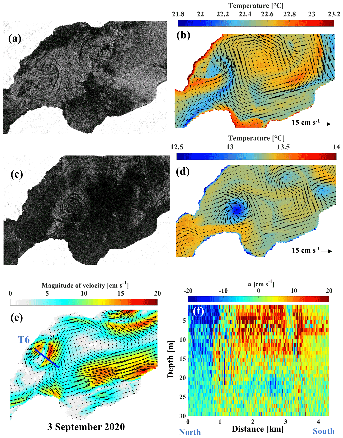
Figure 12 Evidence for the existence of submesoscale eddy 2 (SE2). (a) Remote sensing evidence (SAR image, Sentinel-1) of SE2 for 19 August 2018. (b) Corresponding modelled surface velocity fields (small black arrows) and temperatures shown by colours. (c) SAR image of SE2 for 7 November 2018. (d) Corresponding modelled surface velocity and temperature fields for 7 November 2018. (e) Modelled surface velocity and selected transect (T6) for the field campaign of 3 September 2020. (f) Measured horizontal current velocity along T6. For location of these panels, see Fig. 11c. Colour bars give the range of the parameters in the panels. Positive horizontal velocity points eastward.

5 Discussion

5.1 Proposed procedure for detecting gyres

Large-scale gyres and eddies are important transport processes in large lakes that provide for the rapid spreading of materials from the nearshore zone into the lake interior. The present study proposed a procedure for locating gyres and small eddies in a large lake and also for determining the details of their patterns. Its application to Lake Geneva has shown that a unique relationship exists between Bise wind forcing events and the resulting three-gyre pattern. This pattern is predictable and stable in space and time for a certain period after the forcing has ceased. The subsequent confirmation of the results by transect field measurements whose location and timing was based on the predicted pattern has demonstrated the feasibility and the robustness of the procedure. As a result, strategies for such field campaigns can be designed, ensuring a high success rate in detecting gyres and eddies. Without the information provided by this procedure, it is almost impossible to carry out such field campaigns, given the complex nature of circulation patterns that exist in Lake Geneva as highlighted by the EOF results.

5.2 Gyre pattern: two or three gyres?

Numerical studies have shown that large-scale gyres contribute significantly to the transport of water masses and potential pollutants from the nearshore zone into the interior of the lake (Cimatoribus et al., 2019; Reiss et al., 2020). Particle tracking used in these studies indicated a rapid spreading of these water masses over large areas of the Grand Lac basin within a short time, once they were caught in gyres. Previous numerical simulation studies on Lake Geneva suggested that two basin-scale gyres located at the centre of the deep Grand Lac basin drive the main basin-scale circulation (Le Thi et al., 2012; Lemmin, 2016; Razmi et al., 2017) and can have an impact on lake biological–chemical–physical interactions (Cotte and Vennemann, 2020). However, no field measurements were carried out to confirm the existence of a two-gyre pattern reported in those studies. In the present study, transect field measurements provided detailed evidence of these two gyres.

Furthermore, transect field measurements confirmed the existence of a third gyre located in the eastern part of Grand Lac that is as well developed as the other two gyres. Previously, modelling had suggested that this third gyre may be important for the rapid spreading of water masses and potential pollutants brought into the lake by the Rhône River because its plume directly fed into this gyre (Lemmin, 2016). Generally, the signature of the cyclonic gyres, CG1 in the centre and CG2 in the eastern part of the lake, is more pronounced than that of an anticyclonic gyre, AG, in the west. The western part of the lake is directly exposed to sustained strong winds, in contrast to the topographically sheltered eastern part (Rahaghi et al., 2019; Figs. 5a, 7). Based on the EOF analysis in the proposed procedure, it could be established that, different from previous individual gyre observations, three gyres occur regularly and have a consistent pattern. The link between the three-gyre pattern and wind forcing was made evident. In addition, it was demonstrated that the location of gyre centres and the duration of the gyre pattern only changed slightly between Bise events.

5.3 Forcing: importance of spatial heterogeneity

The dominant role of wind as the primary force in gyre formation, the impact of stratification and Coriolis forcing, and the importance of surface heating and cooling in driving or enhancing gyre flows have recently been highlighted (Hogg and Gayen, 2020). The spatial pattern of the net heat flux suggests that the heterogeneity between heating and cooling in the eastern part of the lake is more significant than in the western part (Fig. 5b). This agrees with findings of spatial heat flux variability by Rahaghi et al. (2019). The variability may impact the strength of gyre flows in the eastern part of Lake Geneva. Further research is needed in order to quantify the role of differential surface buoyancy fluxes on the strength of cyclonic gyres in the eastern part of the lake, particularly during summertime, when diurnal heating and cooling are stronger.

As shown in Fig. 9, the depth influenced by the gyre field (AG) in the western part of the lake is greater than the depths influenced by CG1 located in the centre and CG2 in the eastern part of the lake for the November and October campaigns. The gyre velocity is constrained by the thermocline depth, as previously discussed. The thermocline depth can also be affected by the spatial heterogeneity of atmospheric forcing and gyre motions. Forcing by wind stress, the primary source of energy for mixing the water column, is more pronounced in the western part (Figs. 5a, 7). Consequently, a deeper mixed layer would be expected in the western part of the lake. The lower velocity of gyre flow in the western part of the lake can be attributed to the fact that the wind energy can penetrate into deeper layers due to a deeper thermocline, whereas it is confined by a shallower thermocline in the eastern part. As a result, the maximum velocity field of CG1 and CG2 is generally greater than AG.

In many large water bodies surrounded by complex terrain, a spatially variable wind field is one of the most important driving forces for the excitation of both horizontal and residual circulations (Nakayama et al., 2014). It was suggested, for example, that wind stress curl played a significant role in forming cyclonic and anticyclonic circulations in many lakes, such as Lake Superior (Bennington et al., 2010), Lake Michigan (Schwab and Beletsky, 2003), Lake Kinneret (Israel; Laval et al., 2003), Lake Tahoe (USA; Rueda et al., 2005), and Lake Biwa (Japan; Shimizu et al., 2007). The wind field in Lake Geneva, which is also surrounded by a complex terrain (Fig. 1), can vary spatially, as shown in Fig. 7. The lake surface may experience both positive and negative wind stress curl in different areas as a result of such a variable wind field. Under constant positive (negative) wind stress curl, divergent (convergent) Ekman transport can lead to formation of cyclonic (anticyclonic) circulations. Several areas with positive and negative wind stress curls can be identified on the surface of the lake (Fig. 7b, d, e). In general, the magnitude of positive and negative wind stress curl is greater in nearshore zones than in pelagic areas. The wind stress curl is both positive and negative in the CG1 and CG2 areas. However, it is insignificant or positive at the location of AG. Thus, Ekman pumping cannot be responsible for the formation of the anticyclonic circulation in AG located in the western part of the lake. Positive wind stress curl in the eastern part of the lake may, however, play a role in the excitation of cyclonic circulations (Lemmin and D'Adamo, 1996). Further research is required to quantify the effects of spatial variability in surface heat flux (Rahaghi et al., 2019) and wind stress curl on the development of the three-gyre pattern observed in the field.

5.4 Effect of thermal stratification on the gyre velocity field

Thermal stratification of the water column is subject to seasonal changes and can determine the depth affected by mesoscale and basin-scale gyres. The temporal evolution of the gyre flow field in the vertical direction is investigated based on horizontal velocity contour profiles (u) measured at the centre of CG1 from September to December 2019 (Fig. 13). Since transect T2 (see Fig. 1), located in the centre of CG1, is not exposed to strong wind events, seasonal cooling can be considered to be the primary factor controlling the increase in thermocline depth with time. As a result, the depth of the water column affected by the gyre motions continuously increases from September to December, while the maximum current velocity at near-surface layers diminishes (Fig. 13). The CG1 flow field was found to extend to depths of approximately 15 m in September and 20 m in October, which corresponds to the thermocline layer depth where strong temperature drops of ∼10 and 8 ^∘C, respectively, were observed (Fig. 13).

The gyre flow field penetrated to depths of ∼40 m in November and ∼60 m in December. This is deeper than the depth at which the thermocline layer began to form. For November and December, the temperature drops in the thermocline layer were ∼4 and ∼3 ^∘C, respectively. Due to seasonal cooling, the thermocline strength, i.e. the temperature–depth segment connecting a point below the mixed layer and the thermocline depth, decreases from September to December. These observations indicate that the thermocline layer can act as a physical barrier that confines gyre velocity fields in the vertical direction during strongly stratified conditions. Under weak stratification conditions, the gyre velocity field can penetrate into the thermocline layer due to the weakening of this physical barrier. Therefore, the thermocline layer is not an absolute barrier. Furthermore, the temperature profiles measured at the centre and in the nearshore areas of transect T2 indicate that the thermocline can be dome-shaped (Fig. 13). This suggests pelagic upwelling in the centre of the gyre. However, this aspect cannot be treated in detail with the available data and is beyond the scope of the present paper.

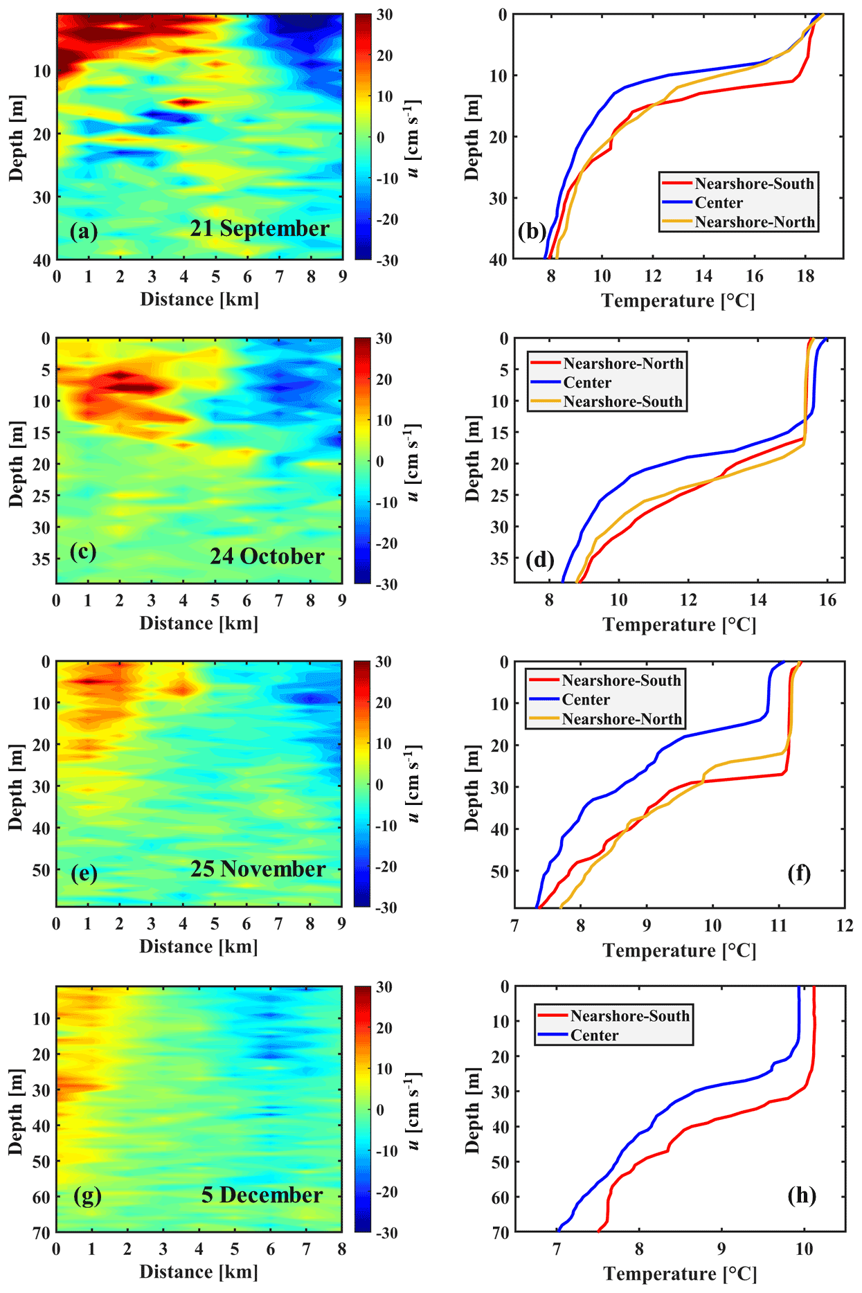
Figure 13 Left column: contour plots of the measured horizontal velocity along Transect T2 (for location, see Fig. 1b). Right column: measured temperature profiles at the locations marked by corresponding coloured triangles above panels in the left column: (a) and (b) 21 September 2019, (c) and (d) 24 October 2019, (e) and (f) 25 November 2019, (g) and (h) 5 December 2019. Note that all panels in the left column are plotted with the same range to highlight the seasonal change; the range of the x axis in the right column changes with time. Colour bars show the range of horizontal velocities.

5.5 Effect of the Coriolis force on the gyre velocity field

To further investigate the effect of Coriolis force on the gyre flows, the vertically averaged horizontal-momentum equation can be written as (Vallis, 2017; Cimatoribus et al., 2018)

$$\begin{array}{}\text{(6)}& {\displaystyle \frac{\partial U_{\mathrm{h}}}{\partial t}}=P+N+C+F-D,\end{array}$$

where U_h is the horizontal velocity field, P is the acceleration induced by the barotropic and baroclinic pressure gradients, N is the acceleration caused by the nonlinear (advection) terms, C is the acceleration caused by the Coriolis force, F is the acceleration induced by external forces, and D is the deceleration induced by dissipation (i.e. bulk, lateral, and bottom friction). The zonal and meridional momentum trends of the Coriolis term (C) are first determined. Then, the magnitude and direction of the temporally averaged horizontal momentum trends induced by C are examined.

During the Bise event from 17 to 20 September 2019, the resultant near-surface currents (depth-averaged over 5 m) are oriented towards the north of the lake, due to Ekman transport (Fig. 14a). After the wind event ceased, the three-gyre system is fully developed (Fig. S3a). The Coriolis force exerts different effects on cyclonic and anticyclonic circulations (Fig. 14b): a bowl-shaped thermocline forms at the centre of the anticyclonic gyre, AG, due to the convergence of the flow field, whereas divergence in the cyclonic CG1 and CG2 flow fields forms dome-shaped thermoclines, as confirmed by the temperature profiles measured during different months at the centre of CG1 (Fig. 13).

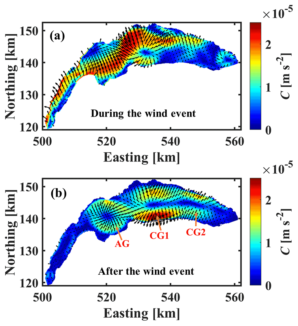
Figure 14 (a) Contribution of Coriolis term C (strength as indicated by colour contours and orientation by arrows) to the vertically (upper 5 m of the water column) and temporally (65 h) averaged horizontal-momentum equation (Eq. 6): (a) during and (b) after the Bise event that occurred in September 2019. After the wind event, convergence can be seen at gyre AG and divergence in the CG1 gyre area.

6 Summary and conclusions

In order to advance the understanding of water mass movement dynamics in large lakes, it is essential to determine the contribution of basin-scale gyres. Therefore, in this study, we developed a novel procedure combining high-resolution 3D numerical simulations, the Okubo–Weiss (OW) parameter, and EOF analysis that can provide direct evidence of the existence of cyclonic (anticlockwise-rotating) and anticyclonic (clockwise-rotating) basin-scale gyres and mesoscale eddies in large lakes. Its feasibility and robustness were assessed and confirmed by field measurements taken in Lake Geneva along transects whose location and timing were based on the numerical-modelling-predicted pattern. The results of this study can be summarized as follows.

The gyre flow field is characterized by a coherent pattern of the normalized Okubo–Weiss parameter, OW_N, in different layers of the lake, as was detected by the EOF analysis. The results showed a clear link between strong large-scale wind events and the computed spatial patterns in the first mode of the EOF analysis. The procedure allowed detection of the location of gyre centres where almost zero horizontal-velocity zones indicate the occurrence of pelagic upwelling or downwelling; this has a great impact on the biological–chemical–physical development of large-lake ecological systems.

Field observations confirmed for the first time that three persistent gyres, two cyclonic gyres and one anticyclonic gyre, regularly formed after strong Bise wind events, as was predicted by the proposed procedure. According to the EOF analysis, the horizontal gyre motion is mainly responsive to the wind stress, whereas the depth of the gyre flow field mainly depends on thermocline depth and strength.

Field observations during October and November 2019 demonstrated that the depth of gyre penetration is greater in the western (anticyclonic gyre) than in the eastern part of the lake (cyclonic gyres). The spatial inhomogeneities in external forcing can lead to significant spatial variability in the gyre velocity field in the western and eastern parts of Lake Geneva.

The proposed procedure can also detect (sub)mesoscale eddies if the resolution of the numerical modelling grid is sufficient. These eddies were predominantly cyclonic, and their diameters were O(4–5 km). They may occur due to flow separation in the vicinity of headlands and embayments. These eddies are transient, but, if trapped between larger-scale gyres, they can remain at a fixed location for several days and can have a lifetime comparable to basin-scale gyres. Their patterns were confirmed by field campaigns that were designed following the proposed procedure.

It was demonstrated that by applying the proposed procedure, it is possible to develop strategies for carrying out detailed transect field studies on gyres with precision in time and space, which previously was not possible.

This study highlighted the significance of 3D processes in large lakes, thus indicating that 1D concepts cannot adequately describe the complex dynamics in such lakes. Additional research is required to investigate gyre- and eddy-formation mechanisms and the role that eddies and large basin-scale gyres play in the interaction of biological–chemical–physical processes. Such large-scale circulations can rapidly spread materials, including pollutants, entering the lake in the nearshore zone into the whole lake and thus affect the long-term ecological system development of large lakes. Although the feasibility and robustness of the proposed procedure was assessed in Lake Geneva, it can be applied to any large lake with a comparable database since it is based on universally valid concepts. It is a powerful tool for designing strategies for detailed field studies and will allow new types of field measurements that can contribute to advancing the understanding of large-lake dynamics.