Implementation and evaluation of the GEOS-Chem chemistry module version 13.1.2 within the Community Earth System Model v2.1

We implement the GEOS-Chem chemistry module as a chemical mechanism in version 2 of the Community Earth System Model (CESM). Our implementation allows the state-of-the-science GEOS-Chem chemistry module to be used with identical emissions, meteorology, and climate feedbacks as the CAM-chem chemistry module within CESM. We use coupling interfaces to allow GEOS-Chem to operate almost unchanged within CESM. Aerosols are converted at each time step between the GEOS-Chem bulk representation and the size-resolved representation of CESM's Modal Aerosol Model (MAM4). Land-type information needed for dry-deposition calculations in GEOS-Chem is communicated through a coupler, allowing online land–atmosphere interactions. Wet scavenging in GEOS-Chem is replaced with the Neu and Prather scheme, and a common emissions approach is developed for both CAM-chem and GEOS-Chem in CESM.

We compare how GEOS-Chem embedded in CESM (C-GC) compares to the existing CAM-chem chemistry option (C-CC) when used to simulate atmospheric chemistry in 2016, with identical meteorology and emissions. We compare the atmospheric composition and deposition tendencies between the two simulations and evaluate the residual differences between C-GC and its use as a stand-alone chemistry transport model in the GEOS-Chem High Performance configuration (S-GC). We find that stratospheric ozone agrees well between the three models, with differences of less than 10 % in the core of the ozone layer, but that ozone in the troposphere is generally lower in C-GC than in either C-CC or S-GC. This is likely due to greater tropospheric concentrations of bromine, although other factors such as water vapor may contribute to lesser or greater extents depending on the region. This difference in tropospheric ozone is not uniform, with tropospheric ozone in C-GC being 30 % lower in the Southern Hemisphere when compared with S-GC but within 10 % in the Northern Hemisphere. This suggests differences in the effects of anthropogenic emissions. Aerosol concentrations in C-GC agree with those in S-GC at low altitudes in the tropics but are over 100 % greater in the upper troposphere due to differences in the representation of convective scavenging. We also find that water vapor concentrations vary substantially between the stand-alone and CESM-implemented version of GEOS-Chem, as the simulated hydrological cycle in CESM diverges from that represented in the source NASA Modern-Era Retrospective analysis for Research and Applications (Version 2; MERRA-2) reanalysis meteorology which is used directly in the GEOS-Chem chemistry transport model (CTM).

Our implementation of GEOS-Chem as a chemistry option in CESM (including full chemistry–climate feedback) is publicly available and is being considered for inclusion in the CESM main code repository. This work is a significant step in the MUlti-Scale Infrastructure for Chemistry and Aerosols (MUSICA) project, enabling two communities of atmospheric researchers (CESM and GEOS-Chem) to share expertise through a common modeling framework, thereby accelerating progress in atmospheric science.

1 Introduction

Accurate representation and understanding of atmospheric chemistry in global Earth system models (ESMs) has been recognized as an urgent priority in geoscientific model development. The National Research Council (NRC) report on a “National Strategy for Advancing Climate Modeling” (National Research Council, 2012) stresses the need to include comprehensive atmospheric chemistry in the next generation of ESMs. The NRC report on the “Future of Atmospheric Chemistry Research” (National Academies of Sciences, Engineering, and Medicine, 2016) identifies the integration of atmospheric chemistry into weather and climate models as one of its five priority science areas. This work responds to those needs, presenting the implementation of the state-of-the-science model GEOS-Chem (Bey et al., 2001; Eastham et al., 2018) as an atmospheric chemistry module within the Community Earth System Model (CESM) (Lamarque et al., 2012; Hurrell et al., 2013; Tilmes et al., 2016; Emmons et al., 2020).

GEOS-Chem is a state-of-the-science global atmospheric chemistry model developed and used by over 150 research groups worldwide (http://geos-chem.org, last access: 21 August 2022). It has wide appeal among atmospheric chemists because it is a comprehensive, state-of-the-science, open-access, well-documented modeling resource that is easy to use and modify but also has strong central management, version control, and user support. The model is managed at Harvard by the GEOS-Chem Support Team with oversight from the international GEOS-Chem Steering Committee. Documentation and communication with users is done through extensive web and wiki pages, email lists, newsletters, and benchmarking. Grassroots model development is done by users, and inclusion into the standard model is prioritized by working groups reporting to the Steering Committee. The model can simulate tropospheric and stratospheric oxidant–aerosol chemistry, aerosol microphysics, and budgets of various gases. Simulations can be conducted on a wide range of computing platforms with either shared-memory (OpenMP) or distributed-memory (MPI) parallelization – with this latter implementation referred to as GEOS-Chem High Performance, or GCHP (Eastham et al., 2018). For the general atmospheric chemistry problem involving K atmospheric species coupled by chemistry and/or aerosol microphysics, GEOS-Chem solves the system of K coupled continuity equations:

$$\begin{array}{}\text{(1)}& {\displaystyle \frac{\partial n_i}{\partial t}}=-\mathrm{\nabla }\cdot \left(n_i\mathit{U}\right)+P_i\left(\mathit{n}\right)-L_i\left(\mathit{n}\right),\end{array}$$

where n = (n₁,…n_K)^T is the number density vector representing the concentrations of the K species, U is the 3-D wind vector, and P_i and L_i are the respective local production and loss terms for species i including emissions, deposition, chemistry, and aerosol physics. The transport term $-\mathrm{\nabla }\cdot \left(n_i\mathit{U}\right)$ includes advection by grid-resolved winds as well as parameterized subgrid turbulent motions (boundary layer mixing, convection). The local term P_i(n)−L_i(n) couples the continuity equations across species through chemical kinetics and aerosol physics.

Standard application of the GEOS-Chem model as originally described by Bey et al. (2001) is offline, meaning that the model does not simulate its own atmospheric dynamics. Instead, it uses analyzed winds and other meteorological variables produced by Goddard Earth Observing System (GEOS) simulations of the NASA Global Modeling and Assimilation Office (GMAO) with assimilated meteorological observations. The near-real-time GEOS Forward Processing (GEOS FP) (Luccesi, 2018) output provides data globally at a horizontal resolution of 0.25^∘ × 0.3125^∘, and Version 2 of the Modern-Era Retrospective analysis for Research and Applications (MERRA-2) (Gelaro et al., 2017) provides data at 0.5^∘ × 0.625^∘. GEOS-Chem simulations can be conducted at that native resolution or at a coarser resolution (by conservative regridding of meteorological fields). Long et al. (2015) developed an online capability for GEOS-Chem to be used as a chemical module in ESMs, with initial application to the GEOS ESM. In that configuration, GEOS-Chem only solves the local terms of the continuity equation

$$\begin{array}{}\text{(2)}& {\displaystyle \frac{\partial n_i}{\partial t}}=P_i\left(\mathit{n}\right)-L_i\left(\mathit{n}\right)\end{array}$$

and delivers the updated concentrations to the ESM for computation of transport through its atmospheric dynamics. Online simulation avoids the need for a meteorological data archive and the associated model transport errors (Jöckel et al., 2001; Yu et al., 2018). It also enables fast coupling between chemistry and dynamics.

Transformation of GEOS-Chem to a grid-independent structure was performed transparently, such that the standard GEOS-Chem model uses the exact same code for online and offline applications. This includes a mature implementation within the GEOS ESM. It was applied recently to a yearlong tropospheric chemistry simulation with ≈ 12 km (cubed-sphere c720) global resolution (Hu et al., 2018), and it is now being used for global atmospheric composition forecasting (Keller et al., 2021). However, the only implementations of GEOS-Chem which are currently publicly available are either designed to run “offline”, driven by archived meteorological data from the NASA GEOS ESM, or operate at a regional scale and do not extend to global simulation (Lin et al., 2020; Feng et al., 2021).

Integration of GEOS-Chem as a chemistry option within an open-access, global ESM responds to the aforementioned calls from the NRC. One of the most widely used open-access ESMs is CESM, which is a fully coupled and state-of-the-science model. It produces its own meteorology based on fixed sea surface temperatures or with a fully interactive ocean model. It can also be nudged to analyzed meteorology, including from GEOS. The CESM configuration with chemistry covering the troposphere and stratosphere is referred to as CAM-chem (Community Atmosphere Model with chemistry) (Lamarque et al., 2012; Tilmes et al., 2016). CAM-chem is a state-of-the-science model of atmospheric chemistry; it has participated (along with CESM's Whole Atmosphere Community Climate Model, WACCM, model which extends to the lower thermosphere) in many international model intercomparison activities, such as the Atmospheric Chemistry and Climate Model Intercomparison Project (ACCMIP), Chemistry-Climate Model Initiative (CCMI), the POLARCAT (Polar Study using Aircraft, Remote Sensing, Surface Measurements and Models, of Climate, Chemistry, Aerosols, and Transport) Model Intercomparison Project (POLMIP), the Hemispheric Transport of Air Pollution effort (HTAP2), the Geoengineering Model Intercomparison Project (GeoMIP), and the Coupled Model Intercomparison Project Phase 6 (CMIP6), and has a large international user community. CAM-chem also has a very different development heritage from GEOS-Chem, with each model providing better performance in comparison to observations in different areas (Emmons et al., 2015; Nicely et al., 2017; Jonson et al., 2018; Park et al., 2021). It is widely used for simulations of global tropospheric and stratospheric atmospheric composition, in part because it is able to run either with specified meteorological datasets or with fully coupled physics (https://www2.acom.ucar.edu/gcm/cam-chem, last access: 16 August 2022).

The fundamental differences in the implementation of almost every atmospheric process between GEOS-Chem and CAM-chem mean that it is difficult to disentangle the root causes of these differences. Modular ESMs can resolve this issue. Allowing individual scientific components to be swapped freely allows researchers to evaluate exactly what effect that component has in isolation while also giving a single user base access to a larger portfolio of options. If two different models each implement five processes in different ways, a researcher must learn to use both in order to compare their results and cannot isolate the effect of any one process with confidence. If process options are implemented in the same framework, this problem is avoided. Such modularity is becoming increasingly possible with the availability of Earth system infrastructure such as the Earth System Modeling Framework (ESMF) and the National Unified Operational Prediction Capability (NUOPC), which describe common interfaces for Earth system modeling components (Hill et al., 2004; Sandgathe et al., 2011). The Multi-Scale Infrastructure for Chemistry and Aerosols (MUSICA) builds upon this trend with process-level modularization, with the goal of allowing researchers to select from a range of community-developed options when performing atmospheric simulations.

This work integrates the GEOS-Chem chemistry module into CESM as an alternative option to CAM-chem. Our implementation allows researchers to select either of the models to simulate gas-phase and aerosol chemistry throughout the troposphere and stratosphere, while other processes such as advection, broadband radiative transfer, convective transport, and emissions are handled nearly identically. We demonstrate this capability by comparing simulations of the year 2016 as generated by GEOS-Chem and CAM-chem operating within CESM, with the chemical module being the only difference. Estimates of atmospheric composition are compared between the two models and against a simulation in the stand-alone GCHP chemistry transport model (CTM). Finally, we evaluate the accuracy of the three approaches against observations of atmospheric composition and deposition.

Section 2 provides a technical description of the implementation of GEOS-Chem into CESM. Section 3 then describes the model setup. Sections 4 and 5 present results from a 1-year simulation (following the appropriate spin-up) performed for each model configuration: (1) CESM with GEOS-Chem, (2) CESM with CAM-chem, and (3) the stand-alone GEOS-Chem CTM. This includes model intercomparison (Sect. 4) and evaluation against surface and satellite measurements (Sect. 5). Finally, discussion and conclusions are provided in Sect. 6.

2 Coupling between GEOS-Chem and CESM

We first describe the interface used within CESM when using either the CAM-chem or GEOS-Chem options (Sect. 2.1). Unless otherwise stated, “GEOS-Chem” refers to the grid-independent chemistry module which is common to all implementations, including stand-alone GEOS-Chem with OpenMP (Classic) or MPI (GCHP) parallelization, NASA GMAO's GEOS ESM, and the Weather Research and Forecasting (WRF) model coupled with GEOS-Chem (WRF-GC). We then briefly summarize the chemistry and processes represented by the CAM-chem and GEOS-Chem options within CESM (Sect. 2.2). This is followed by a description of differences between the implementation of GEOS-Chem in CESM and its stand-alone code (Sect. 2.3), differences in the data flow through CESM when using GEOS-Chem as opposed to CAM-chem (Sect. 2.4), and finally the installation and compilation process (Sect. 2.5).

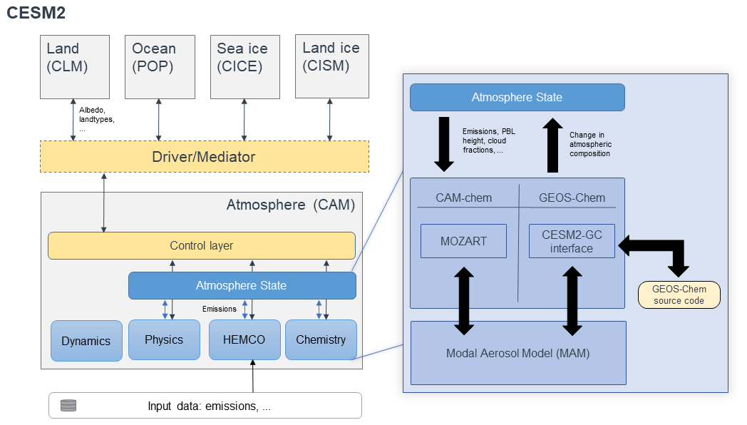
Figure 1 Architectural overview of CESM when running with either the GEOS-Chem or CAM-chem chemistry options. The left section shows the architecture of CESM, where the five major Earth system components are connected through the driver/mediator. The work presented here changes only the contents of the atmosphere component (CAM). Regardless of the chemistry option used, dynamics, physics, and emissions (HEMCO) are handled identically. Each component modifies the “Atmosphere State” while communication occurs through the control layer. The choice of chemistry module is confined to the “Chemistry” subcomponent, where either CAM-chem or GEOS-Chem can be chosen. In each case, data are transmitted between the Atmosphere State and the chemistry module, which interacts in turn with the Modal Aerosol Model. Dynamics are shown separately, as they act on a “dynamics container” rather than directly on the atmospheric state. Further detail regarding the timing of calls is provided in the Supplement.

2.1 Interface

Our approach embeds a full copy of the GEOS-Chem chemistry module source code (version 13.1.2) within CESM (version 2.1.1). All modifications made to the GEOS-Chem source code have been propagated to the GEOS-Chem main code branch (https://github.com/geoschem/geos-chem, last access: 16 August 2022) to ensure future compatibility between CESM and GEOS-Chem. Information is passed between the CESM Community Atmosphere Model (CAM) version 6 (CAM6) and the GEOS-Chem routines through an interface layer developed as part of this work. A schematic representation of the implementation is provided in Fig. 1.

At each time step, CESM calls the coupling interface (referred to as “CESM2-GC interface” in Fig. 1) that fills in the meteorological variables required by either CAM-chem or GEOS-Chem. Atmospheric transport and physics are identical whether using CAM-chem or GEOS-Chem to simulate atmospheric chemistry. The interface passes species concentrations from CAM to GEOS-Chem, which are then modified by GEOS-Chem and passed back to CAM. Meteorological data and land data are also passed to GEOS-Chem through the same interface. The routine calls in CAM when using either GEOS-Chem or CAM-chem are identical, with the appropriate chemistry module defined at the compilation time such that the calls are routed to the appropriate routines.

The interface handles the conversion of meteorological variables and concentrations of atmospheric constituents between the state variables in CAM and those used in GEOS-Chem. As GEOS-Chem operates in a grid-independent fashion, changes in the grid specification and other upstream modifications to CESM do not necessitate any changes to this interface (Long et al., 2015). Our version of CESM 2.1.1 is modified such that emissions are handled by the Harmonized Emissions Component (HEMCO) (Keller et al., 2014), which operates independently of the chemistry module and can provide emissions data to either CAM-chem or GEOS-Chem equally (Lin et al., 2021).

The interface code is kept in a subfolder of chemistry source code (src/chemistry/geoschem subfolder), which also contains a copy of the source code for GEOS-Chem. Unlike the implementation of GEOS-Chem within GEOS, we do not use ESMF. However, we plan to develop a NUOPC-based interface as part of future work.

2.2 Processes represented by CAM-chem and GEOS-Chem

CAM-chem uses the Model for OZone And Related chemical Tracers (MOZART) family of chemical mechanisms to simulate atmospheric chemistry (Emmons et al., 2020). The tropospheric–stratospheric MOZART-TS1 scheme that we demonstrate in our intercomparison involves 186 gas-phase chemical species and includes stratospheric bromine and chlorine chemistry. MOZART-TS1 does not include detailed tropospheric halogen chemistry or short-lived halogen sources such as sea-salt bromine, although these will be available in a future release (Badia et al., 2021; Fernandez et al., 2021). Photolysis rates are calculated using a lookup table, based on calculations with the Tropospheric Ultraviolet and Visible (TUV) radiation model (Kinnison et al., 2007). Wet deposition is calculated using the “Neu scheme” (Neu and Prather, 2012) for both convective and large-scale precipitation. Dry-deposition velocities over land are calculated for each land type by the Community Land Model (CLM) in CESM using the Wesely (1989) resistance scheme with updates described by Emmons et al. (2020). Deposition velocities over the ocean are calculated separately in CAM-chem. Aerosols are represented using the four-mode Modal Aerosol Model (MAM4), which includes sulfate, black carbon, primary organic aerosols, and secondary organic aerosols (SOAs) (Mills et al., 2016). Ammonium and ammonium nitrate aerosols are calculated with a parameterization using the bulk aerosol scheme (Tilmes et al., 2016). SOAs are simulated using a five-bin volatility basis set (VBS) scheme, formed from terpenes, isoprene, specific aromatics, and lumped alkanes through reaction with the hydroxyl radical (OH), ozone, and the nitrate radical (NO₃), with unique yields for each combination of volatility and size bin (Tilmes et al., 2019). This more detailed scheme differs from the default MAM SOA scheme that is used in CAM6 (without interactive chemistry). Aerosol deposition, including dry and wet deposition, and gravitational settling (throughout the atmosphere) are calculated in the MAM code of CESM. CAM-chem also uses a VBS approach for SOA with five volatility bins, covering saturation concentrations with logarithmic spacing from 0.01 to 100 µg m⁻³. CAM-chem explicitly represents Aitken- and accumulation-mode SOA using two separate tracers for each volatility bin but does not include an explicit representation of non-volatile aerosol.

GEOS-Chem uses a set of chemical mechanisms implemented with the Kinetic PreProcessor (KPP) (Damian et al., 2002). The standard chemical mechanism has evolved continuously from the tropospheric gas-phase scheme described by Bey et al. (2001) and now includes aerosol chemistry (Park, 2004), stratospheric chemistry (Eastham et al., 2014), and a sophisticated tropospheric–stratospheric halogen chemistry scheme (Wang et al., 2019). The scheme present in GEOS-Chem 13.1.2 includes 299 chemical species. Additional “specialty simulations”, such as an aerosol-only option and a simulation of the global mercury cycle, are present in GEOS-Chem but are not implemented in CESM in this work. Photolysis rates are calculated using the Fast-JX v7 model (Wild et al., 2000). When implemented as the stand-alone model, wet deposition is calculated for large-scale precipitation using separate approaches for water-soluble aerosols (Liu et al., 2001) and gases (Amos et al., 2012) with calculation of convective scavenging performed inline with convective transport. A different approach is used to simulate wet scavenging for the implementation of GEOS-Chem in CESM (see Sect. 2.3.4). Dry deposition is calculated using the Wesely (1989) scheme (Wang et al., 1998) but with updates for nitric acid (HNO₃) (Jaeglé et al., 2018), aerosols (Zhang et al., 2001; Alexander et al., 2005; Fairlie et al., 2007; Jaeglé et al., 2011), and over the ocean (Pound et al., 2020). The representation of aerosols in GEOS-Chem varies by species. Sulfate–ammonium–nitrate aerosol is represented using a bulk scheme (Park, 2004), with gas–particle partitioning determined using ISORROPIA II (Fountoukis and Nenes, 2007). Modal and sectional size-resolved aerosol schemes are available for GEOS-Chem (Kodros and Pierce, 2017; Yu and Luo, 2009), but they are disabled by default and are not used in this work. Sea-salt aerosol is represented using two (fine and coarse) modes (Jaeglé et al., 2011), whereas dust is represented using four size bins (Fairlie et al., 2007). We use the “complex SOA” chemistry mechanism in GEOS-Chem when running in CESM, as this uses a VBS representation of SOA which is broadly compatible with that used in CAM-chem (Pye et al., 2010; Pye and Seinfeld, 2010; Marais et al., 2016). The complex SOA VBS scheme uses four volatility bins covering saturation concentrations on a logarithmic scale from 0.1 to 100 µg m⁻³. Two classes of SOA are represented in this fashion: those derived from terpenes (TSOA) and those derived from aromatics (ASOA). For each “class” of SOA, two tracers are used to represent each volatility bin (one holding the gas-phase mass and the other holding the condensed-phase mass). The only exception is the lowest-volatility aromatic aerosol, which is considered to be non-volatile and, therefore, has no gas-phase tracer. Two additional SOA tracers, representing isoprene-derived and glyoxal-derived SOA, are not represented using a VBS approach.

Additional differences between the two chemistry modules include the use of different Henry's law coefficients, gravitational settling schemes, representation of polar stratospheric clouds, and heterogeneous chemistry. Full descriptions of the two models are available at https://geos-chem.seas.harvard.edu/ (last access: 16 August 2022) and in Emmons et al. (2020).

2.3 Representation of atmospheric processes in GEOS-Chem when running in CESM

Some processes cannot be easily transferred from the stand-alone GEOS-Chem model to its implementation in CESM, due to factors such as the different splitting of convective transport in the two models. Processes that vary in their implementation between the stand-alone model and the CESM implementations of GEOS-Chem are described below.

2.3.1 Aerosol coupling in CESM with GEOS-Chem

As GEOS-Chem and CESM use different approaches to represent aerosols, there is no straightforward translation between the GEOS-Chem representation and that used elsewhere in CESM. We implement an interface between the CESM and GEOS-Chem representations, so that GEOS-Chem's processing of aerosols is most accurately represented without compromising the microphysical simulations and radiative interactions of aerosol calculated elsewhere in CESM.

CESM uses MAM4 to represent the aerosol size distribution and perform aerosol microphysics (Liu et al., 2016). This represents the mass of sulfate aerosols, secondary organic matter (in five volatility basis set bins), primary organic matter, black carbon, soil dust, and sea salt with advected tracers in four modes (accumulation, Aitken, coarse, and primary carbon), although some species are considered only in a subset of the four modes. A tracer is also implemented for the number of aerosol particles in each mode, resulting in a total of 18 tracers. As discussed above, GEOS-Chem instead represents sulfate, nitrate, and ammonium aerosol constituents with three tracers; fresh and aged black and organic carbon with four tracers; fine and coarse sea salt as two tracers; and different sizes of dust with four tracers. Six additional tracers are used to track the bromine, iodine, and chlorine content of each mode of sea-salt aerosol, with two more used to track overall alkalinity. Gas-phase sulfuric acid (H₂SO₄) is assumed to be negligible in the troposphere and is estimated using an equilibrium calculation in the stratosphere (Eastham et al., 2014). Therefore, the GEOS-Chem mechanism represents greater chemical complexity but reduced size resolution compared with the aerosol representation in MAM4.

Accordingly, when receiving species concentrations from CESM, the interface to GEOS-Chem lumps all modes of the MAM aerosol into the corresponding GEOS-Chem tracer. This includes gas-phase H₂SO₄, in the case of the GEOS-Chem sulfate (SO₄) tracer. Aerosol constituents which are not represented explicitly by MAM (e.g., nitrates) are not included in this calculation. The relative contribution of each mode is stored during this “lumping” process for each grid cell. Once calculations with GEOS-Chem are complete, the updated concentration of the lumped aerosol is repartitioned into the MAM tracers based on the stored relative contributions in each grid cell.

Table 1 Mapping between tracers used to represent SOA in GEOS-Chem and CAM-chem. Translation between GEOS-Chem and MAM4 is performed by preserving the relative contributions provided during the previous transfer.

TSOG represents semivolatile gas products of monoterpenes and sesquiterpene oxidation (GEOS-Chem), ASOG represents lumped semivolatile gas products of light aromatics (GEOS-Chem), and SOAG represents oxygenated volatile organic compounds (CESM).

For SOAs, additional steps are needed. For the bins covering saturation concentrations of 1 µg m⁻³ and greater, we assume that the relevant volatility bin in MAM4 is equal to the sum of the two classes in GEOS-Chem covering the same saturation concentrations. For example, the tracers TSOA1 and ASOA1 in GEOS-Chem are combined to estimate the total quantity of the Aitken and accumulation modes for species “soa3” in MAM4. Partitioning between the two modes (when transferring from GEOS-Chem to MAM4) is calculated based on the relative contribution of each constituent to the total prior to processing by GEOS-Chem. Partitioning between the two classes (when transferring from MAM4 to GEOS-Chem) is calculated based on the relative contribution of each constituent to the total at the end of the previous time step. For the lowest-volatility species, we split the lowest volatility bin concentrations (and non-volatile species) from GEOS-Chem between the two lowest volatilities in MAM4. A full mapping for all species is provided in Table 1.

Finally, MAM simulates some chemical processing on and in the aerosol. This includes the reaction of sulfur dioxide with hydrogen peroxide and ozone in clouds, which is already included in the GEOS-Chem chemistry mechanism. Therefore, we disable in-cloud sulfur oxidation in MAM4 when using the GEOS-Chem chemistry component in CESM, consistent with the GEOS-Chem CTM. A comparison of the effect of each approach is provided in the Supplement.

2.3.2 Dry deposition

Dry-deposition velocities over land are calculated in CESM for each atmospheric constituent by the Community Land Model (CLM) using a species database stored by the coupler. GEOS-Chem is also able to calculate its own dry-deposition velocities (see Sect. 2.2) in situations where a land model is not available, such as when running as a CTM. Thus, we implement different options to compute dry-deposition velocities when running CESM with the GEOS-Chem chemistry option:

1. Dry-deposition velocities over land are computed by CLM and are passed to CAM through the coupler. They are then merged with dry-deposition velocities computed over ocean and ice by GEOS-Chem, identical to the procedure used in CAM-chem. Each of these are scaled by the land and ocean/ice fraction, respectively.

2. GEOS-Chem computes dry deposition at any location using the land types and leaf area indices from CLM, which are passed through the coupler.

3. GEOS-Chem obtains “offline” land types and leaf area indices and computes the dry-deposition velocities similarly to GEOS-Chem Classic.

This allows researchers to experiment with different dry-deposition options, ranging from that most consistent with the approach used in CAM-chem (option 1) to that most consistent with stand-alone GEOS-Chem (option 3). For this work, we use option 2, but option 1 will be included as standard in the CESM main code to reduce data transfer requirements.

2.3.3 Emissions

The Harmonized Emissions Component (HEMCO) is used to calculate emissions in the stand-alone GEOS-Chem model (Keller et al., 2014), and HEMCO v3.0 was recently implemented as an option for CAM-chem (Lin et al., 2021). HEMCO offers the possibility for the user to read, regrid, overlay, and scale emission fluxes from different archived emissions inventories at runtime. Emissions extensions allow for the computation of emissions that depend on meteorology or surface characteristics (e.g., lightning or dust emissions). Some extensions have also been designed to calculate subgrid-scale chemical processes, such as non-linear chemistry in ship plumes (Vinken et al., 2011).

The GEOS-Chem CTM implementations use archived (“offline”) inventories of natural emissions, calculated at their native resolution using the NASA GEOS MERRA-2 and GEOS FP meteorological fields. This ensures that the emissions are calculated consistently regardless of grid resolution. These archived emissions fields can be used within CESM, but we also preserve the option for users to employ “online” emissions inventories where relevant. This enables feedback between climate and emissions to be calculated. For instance, lightning nitrogen oxides (NO_x = nitric oxide (NO) + nitrogen dioxide (NO₂) emissions), dust and sea-salt emissions, and biogenic emissions are all computed online using parameterizations from CAM and CLM. CAM computes lightning NO_x emissions based on the lightning flash frequency, which is estimated following the model cloud height, with different parameterizations over ocean and land. The NO lightning production rate in CAM is assumed to be proportional to the discharged energy, with 10¹⁷ atoms of nitrogen released per joule (Price et al., 1997). The lightning NO_x emissions are then allocated vertically from the surface to the local cloud top based on the distribution described by Pickering et al. (1998). For biogenic emissions, we use the online Model of Emissions of Gases and Aerosols from Nature version 2.1 (MEGANv2.1), as established in CLM (Guenther et al., 2012). Aerosol mass and number emissions are passed directly to MAM constituents. Global anthropogenic emissions can be specified from any of the standard GEOS-Chem inventories, but they default to the Community Emissions Data System (CEDS) inventory (Hoesly et al., 2018). Sulfur emissions from the CEDS inventory are partitioned into size-resolved aerosol (mass and number) and sulfur dioxide (SO₂) (Emmons et al., 2020). In CAM, volcanic out-gassing of SO₂ is provided from the Global Emissions Inventory Activity (GEIA) inventory, with 2.5 % emitted as sulfate aerosol (Andres and Kasgnoc, 1998), whereas eruptive emissions are provided from the VolcanEESM database (Neely and Schmidt, 2016). The option is also available through HEMCO to use the “AeroCom” volcanic emissions, which are derived from Ozone Monitoring Instrument (OMI) observations of SO₂ (Carn et al., 2015; Ge et al., 2016).

Although we use HEMCO with both model configurations, differences remain between the representation of emissions in CAM-chem and in GEOS-Chem when run within CESM. This is because of differences in the species which are present in their respective mechanisms. For instance, emissions of iodocarbons (CH₃I, CH₂I₂, CH₂ICl, CH₂IBr) and inorganic iodine (HOI, I₂) are not available in CAM-chem because iodine species and chemistry are not explicitly modeled in the versions of CAM-chem available in CESM v2.1.1. Volatile organic compound (VOC) lumping is also performed differently (see the Supplement for more detail).

Where the emitted species are present in both chemical mechanisms, the emissions calculated by HEMCO in CESM are identical whether running with GEOS-Chem or CAM-chem. If the HEMCO implementations of lightning, dust, sea-salt, and biogenic emissions are used, emissions will be identical between CESM and the stand-alone GEOS-Chem CTM.

2.3.4 Wet deposition and convection

For both GEOS-Chem and CAM-chem within CESM, convective scavenging and transport are handled separately. Unlike in the Liu et al. (2001) approach implemented in the GEOS-Chem stand-alone code, removal of soluble gases within convective updrafts is not explicitly simulated in either CAM-chem or GEOS-Chem when embedded in CESM. When using the CAM-chem mechanism within CESM, the Neu scheme is used to perform washout of soluble gaseous species, whereas wet deposition of MAM aerosols is handled by MAM. When running CESM with the GEOS-Chem chemistry mechanism, the Neu scheme also performs wet scavenging for aerosols that are not represented by MAM4 (e.g., nitrate). For all such aerosols, we assume a Henry's law coefficient equal to that for HNO₃.

2.3.5 Surface boundary conditions

In CESM, surface boundary mixing ratios of long-lived greenhouse gases (methane, CH₄; nitrous oxide, N₂O; and chlorofluorocarbons, CFCs) are set to the fields specified for CMIP6 historical conditions and future scenarios (Meinshausen et al., 2017). For whichever CMIP6 scenario is chosen, the boundary conditions overwrite those set by the GEOS-Chem chemistry module or by the HEMCO emissions component.

2.4 Changes to the data flow in CESM when running with GEOS-Chem

In CESM, data such as the Henry's law coefficients required to calculate dry-deposition velocities and wet-scavenging rates for each species are defined at the compile time. For species that are common to GEOS-Chem and CAM-chem but where these factors differ, the GEOS-chem values are used by default. The CAM-chem values are listed alongside them in the source code to allow users to switch if desired. Additionally, we modify CAM, CLM, and the Common Infrastructure for Modeling the Earth (CIME) such that the land model can pass land-type information and leaf area indices to the atmosphere model to compute dry-deposition velocities. This could be a potential solution for dry deposition of aerosols in MAM, which currently uses fixed land types independent of the ones used in CLM (Liu et al., 2012). However, this comes at the cost of passing land information through the coupler at every time step.

2.5 Installation and compilation process

The interface between CESM and GEOS-Chem, as well as the GEOS-Chem source code, is automatically downloaded when CAM checks out its external repositories. The versions of GEOS-Chem and of the coupling interface can be changed by modifying the “Externals_CAM.cfg” and by running the “checkout_externals” command.

When creating a new case, the user chooses the atmospheric chemistry mechanism (GEOS-Chem or CAM-chem). The chemistry option is defined by the name of the CESM configuration (component set, or “compset”), making the process of creating a run directory almost identical when choosing either GEOS-Chem or CAM-chem. Whereas chemistry options in CAM-chem are set explicitly using namelist files, certain options in GEOS-Chem are set using ASCII text input files, which are read during the initialization sequence. Therefore, the installation and build infrastructure of CIME will copy any GEOS-Chem-specific text input files to the case directory when setting up a simulation that includes GEOS-Chem. This currently includes emissions specifications read by HEMCO, although this is expected to change as HEMCO becomes the standard emissions option for both CAM-chem and GEOS-Chem in CESM (currently being discussed with the CESM team).

Although CESM supports both shared-memory parallelization (OpenMP) and distributed-memory parallelization (MPI), GEOS-Chem implemented in CESM does not currently support OpenMP. When running CESM with the GEOS-Chem chemistry model, the number of OpenMP threads per MPI task is therefore set to one.

While a complete copy of the GEOS-Chem source code is downloaded from the version-controlled remote of the GEOS-Chem repository (to ensure that the most-recent release of GEOS-Chem is used), not all files present in the GEOS-Chem source code directory are compiled. For instance, the files pertaining to the GEOS-Chem advection scheme are not needed, as advection is performed by CAM; therefore, the GEOS-Chem advection routines are not compiled. To do this, we implement a new feature in CIME to use “.exclude” files, which list files not needed during compilation. CIME reads each .exclude file at compile time and searches subdirectories recursively from the location of the .exclude file, preventing any named file from being included in compilation. For example, an .exclude file is provided in the chemistry coupling interface folder for GEOS-Chem that lists the files to exclude in the GEOS-Chem source code directories.

3 The setup used for model evaluation

We simulate a 2-year period with GEOS-Chem embedded in CESM (hereafter C-GC). The simulation setup is described in the present section. We then perform a comparison of its output to that generated by two conventional model configurations: one of CESM CAM-chem (hereafter C-CC) and one of stand-alone GEOS-Chem (S-GC) (Sect. 4). By comparing the results produced for the same period between C-CC and C-GC, we can perform the first comparison of GEOS-Chem and CAM-chem when run as chemistry modules within the same ESM. Any differences between these two simulations can only be the result of differences between the two chemical modules and their implementations in CESM. This includes not only differences in the gas-phase chemical mechanism, but also in the implementation of photolysis calculations, heterogeneous chemistry, aerosol microphysics, and the chemical kinetics integrator itself. We also compare output to that produced by the stand-alone GEOS-Chem High Performance model (hereafter S-GC). This enables us to evaluate the effect of using CESM's grid discretization, advection, aerosols, and representation of meteorology compared with that used in the GEOS-Chem CTM.

Lastly, we evaluate the performance of C-GC by comparing model output to observational data (Sect. 5). We also include comparisons of model output from the C-CC and S-GC configurations, to provide insight into the relative performance of the model and the root cause of disagreements with observations. This section (Sect. 3) describes the model configurations in detail, but a brief summary is provided in Table 6.

Following a model spin-up period (6 months for S-GC and 1 year for C-GC and C-CC), the 1-year period of 1 January to 31 December 2016 is simulated and used for multi-model evaluation. For C-CC, the standard restart file provided with CESM is used to provide initial conditions. For S-GC, we use a restart file provided with version 13.1.2 of the GEOS-Chem chemistry module, which was obtained from a 10-year simulation. The CESM restart file is intended to represent the early 21st century, so we have followed the lead of previous studies which have used a 1- to 2-year spin-up period (He et al., 2015; Schwantes et al., 2022). For C-GC, we use initial conditions that are taken from the S-GC restart file where possible, but we fill missing species (e.g., MAM4 aerosol tracers) using data from the C-CC restart file. Both simulations performed with CESM v2.1.1 (C-GC and C-CC) use a horizontal resolution of 1.9^∘ × 2.5^∘ on 56 hybrid pressure levels, extending from the surface to 1.65 hPa. Aerosols are represented in CESM using the four-mode version of the modal aerosol model, MAM4 (Liu et al., 2012). In C-GC, we use the complex SOA chemistry scheme (Pye and Seinfeld, 2010; Pye et al., 2010; Marais et al., 2016). In C-CC, we use the MOZART-TS1 chemistry scheme (Emmons et al., 2020).

Stand-alone GEOS-Chem (S-GC) simulations are performed with the GEOS-Chem High Performance (GCHP) configuration, using a C48 cubed-sphere grid (approximately equivalent to a 2^∘ × 2.5^∘ horizontal grid) on 72 hybrid pressure levels extending up to 0.01 hPa. In GCHP, chemistry is performed up to the stratopause at 1 hPa (approximately 50 km) with simplified parameterizations used above that point. Aerosols are represented using GEOS-Chem's “native” scheme, without translation to or from MAM4. As in C-GC, we use the complex SOA scheme.

All three model configurations are driven using meteorological data from MERRA-2. In S-GC, all meteorological fields are explicitly specified by MERRA-2, using the same 72-layer vertical grid. The only exception is the specific humidity in the stratosphere, which is computed online. In C-CC and C-GC, we use the “specified dynamics” (SD) configuration of CAM6 in which 3-D temperature, 3-D wind velocities, surface pressure, surface temperature, surface sensible heat flux, surface latent heat flux, surface water flux, and surface stresses are provided by MERRA-2. The upper 16 layers from MERRA-2 are removed, leaving a truncated 56-layer vertical grid which is used unmodified by CAM6. These variables are nudged with a relaxation time of 50 h, resulting in a relatively “loose” nudging strength. All other fields (e.g., cloud fraction) are computed using the CAM physics routines; this includes convection. Whereas S-GC computes convective transport from archived convective mass fluxes and calculates scavenging within the updraft (Wu et al., 2007), convective transport in both C-CC and C-GC is calculated in CAM6 using the Clouds Layers Unified By Binomials – SubGrid-Scale (CLUBB-SGS) scheme for shallow convection (Bogenschutz et al., 2013) and the Zhang–McFarlane scheme (Zhang and McFarlane, 1995) for deep convection. Scavenging within the convective updraft is not simulated explicitly.

Water vapor in C-GC is initialized from the specific humidity “Q” restart variable, which is identical to the one used for C-CC; after this point, humidity is calculated based on the moist processes represented explicitly in CAM's physics package. The GEOS-Chem CTM does not calculate water vapor in the troposphere, instead prescribing specific humidity directly from MERRA-2 output. Therefore, mixing ratios of water vapor in C-CC and C-GC are identical to that in S-GC at initialization time, but they may diverge from that point onwards.

Emissions are harmonized between the three models, with all three configurations using HEMCO to calculate emissions fluxes. Surface anthropogenic emissions are provided from CEDS (Hoesly et al., 2018) and are identical between all three models, apart from small differences in effective emissions from ships due to parameterized plume processing (Vinken et al., 2011). Simulated anthropogenic and biomass burning surface emissions of nitrogen oxides are 128–132 Tg (N) in each of the three models. Aviation emissions are calculated in all three models based on the Aviation Emissions Inventory Code (AEIC) 2005 emission inventory, contributing a further 0.8 Tg (N) in addition to other species (Simone et al., 2013).

Lightning emissions are calculated in C-CC and C-GC using the online parameterization described in Sect. 2.3.3, whereas lightning emissions in S-GC are calculated using archived flash densities and cloud-top heights (Murray et al., 2012). Total lightning NO_x emissions are 5.7–6.1 Tg (N) in all three models. A summary of the breakdown of NO_x emissions is provided in Table 2.

Table 2 Annual global anthropogenic, soil, and lightning NO_x emissions expressed in teragrams of nitrogen per year (Tg (N) yr⁻¹).

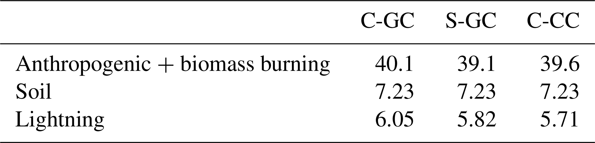
Table 3 Annual global biogenic emission totals in GEOS-Chem implemented in CESM (C-GC) compared with the stand-alone GEOS-Chem (S-GC) model.

Biogenic emissions are calculated in C-CC and C-GC using the embedded MEGAN emissions module in CESM, which differs slightly from the implementation in S-GC and will produce different emissions due to different vegetation distributions. Total biogenic emissions in S-GC and C-GC are shown in Table 3. In all three simulations, we use the AeroCom volcano emissions implemented in HEMCO (Carn et al., 2015).

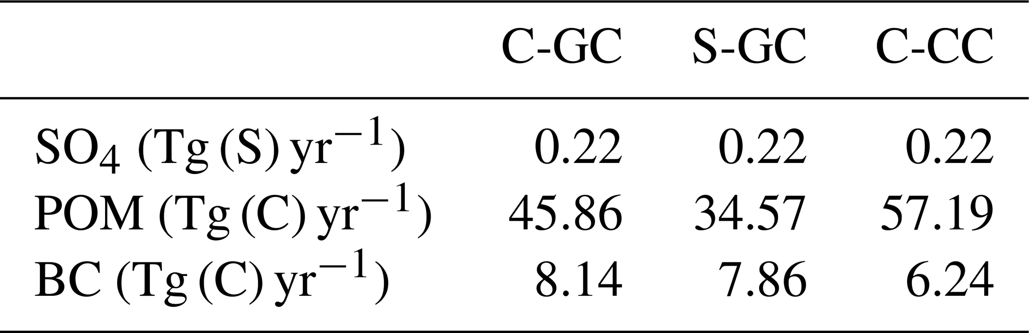
Emissions of aerosols (primary organic matter and black carbon) are listed in Table 4. These emissions are consistent with the values provided in Tilmes et al. (2016).

Table 4 Annual global emissions of sulfates (SO₄), primary organic matter (POM), and black carbon (BS) in all three model configurations.

Mobilization of mineral dust is calculated in all three models using the Dust Entrainment and Deposition (DEAD) scheme (Zender, 2003). In C-CC and C-GC, the online implementation in CESM is employed, resulting in total natural mineral dust emissions of 5984 Tg yr⁻¹. A brief discussion of dust emissions in CESM is provided in the Supplement. In S-GC, natural mineral dust emissions are calculated online using the same scheme but with a different scaling and at a slightly different grid resolution, resulting in total emissions of 1390 Tg yr⁻¹.

Table 5 Annual global emissions of sea-salt aerosols (fine and coarse) and bromine in sea salt for C-GC and S-GC. The names of the tracers used to represent these species in GEOS-Chem are provided in parentheses.

Emissions of sea salt are calculated online in CESM for C-GC and C-CC, whereas S-GC uses a precalculated (offline) inventory of sea-salt emissions, as well as sea-salt bromine and chloride. Emissions of sea-salt bromine in C-GC are calculated based on the offline inventory rather than the calculated emissions of sea salt and, therefore, do not scale correctly with the estimated sea-salt emissions from CESM (see Table 5). This will be resolved as part of future work.

Table 6 Brief summary of the model configuration used for C-GC, S-GC, and C-CC.

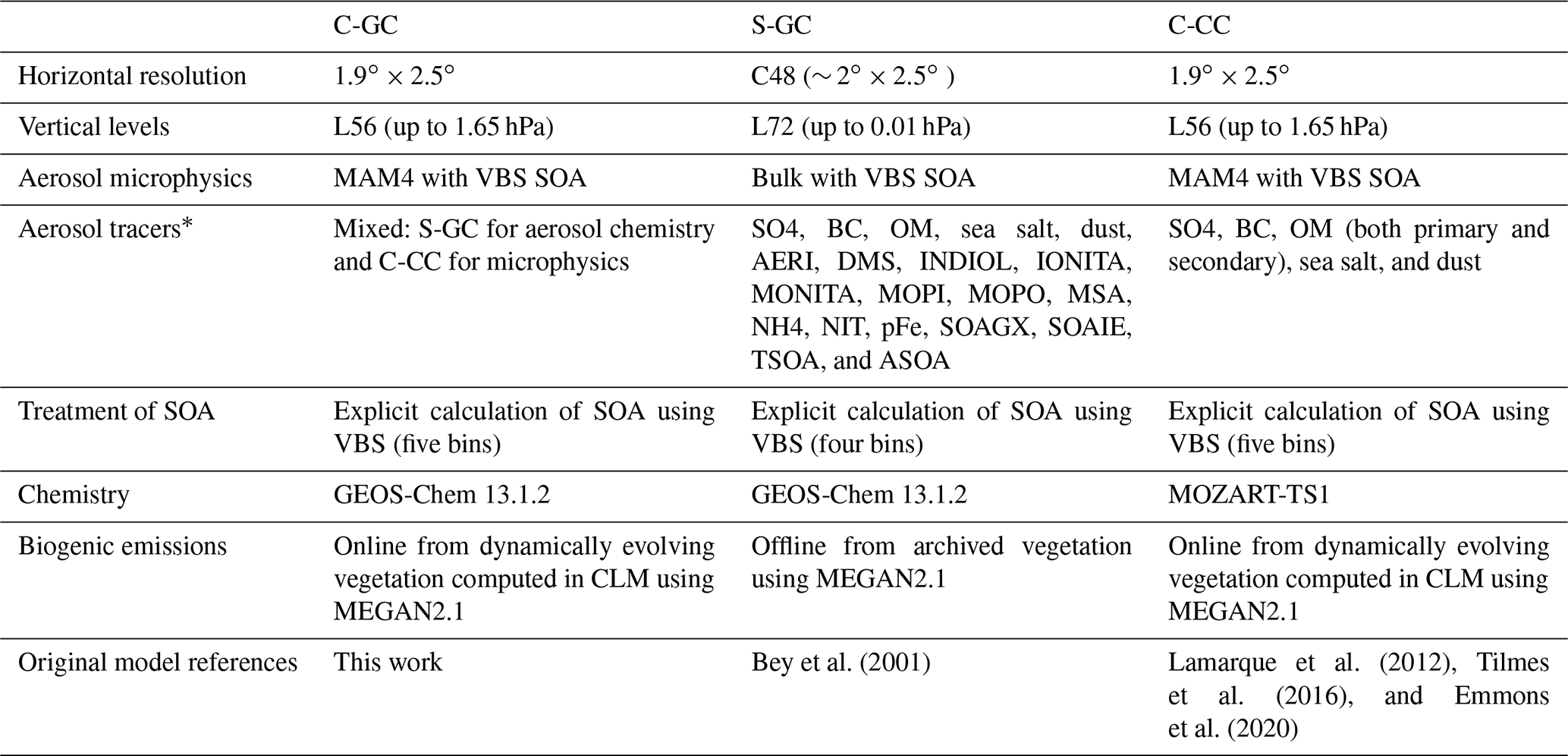
^*For the GEOS-Chem aerosol tracer definitions, the reader is referred to http://wiki.seas.harvard.edu/geos-chem/index.php/Species_in_GEOS-Chem (last access: 24 November 2022).

Finally, for long-lived species, such as CFCs, we use the Shared Socioeconomic Pathway 2-4.5 (SSP2-4.5) (Riahi et al., 2017) set of surface boundary conditions in both C-GC and C-CC. In comparisons against S-GC, we use historical emissions from the World Meteorological Organization's 2018 assessment of ozone depletion (Fahey et al., 2018). However, this difference is unlikely to significantly affect simulation output given the short duration of the simulations.

4 Model intercomparison

We first compare the global distribution of ozone and aerosols among C-GC, S-GC, and C-CC. Section 4.1 evaluates the vertical and latitudinal distribution of ozone and two related species (water vapor, H₂O, and the hydroxyl radical, OH), followed by the global distribution of ozone at the surface in each model configuration (Sect. 4.2). Stratospheric chemistry in GEOS-Chem is described by Eastham et al. (2014) and by Emmons et al. (2020) for CAM-chem. A similar evaluation of differences in zonal mean and surface aerosol concentrations follows (Sect. 4.3).

To understand the causes of these differences, we compare the global distribution of reactive nitrogen and halogen species in each model configuration (Sect. 4.4). When comparing halogen distributions, we consider only bromine and chlorine distributions, as iodine is not simulated in this version of CAM-chem. The latest implementation of halogen chemistry in GEOS-Chem and its role in atmospheric chemistry are described by Wang et al. (2021), while its representation in CAM-chem is described by Emmons et al. (2020). Differences in the total atmospheric burden and vertical distribution of these families provides information regarding differences in removal processes. Differences in their internal partitioning (e.g., between NO_x and HNO₃) provide information regarding the representation of atmospheric chemistry.

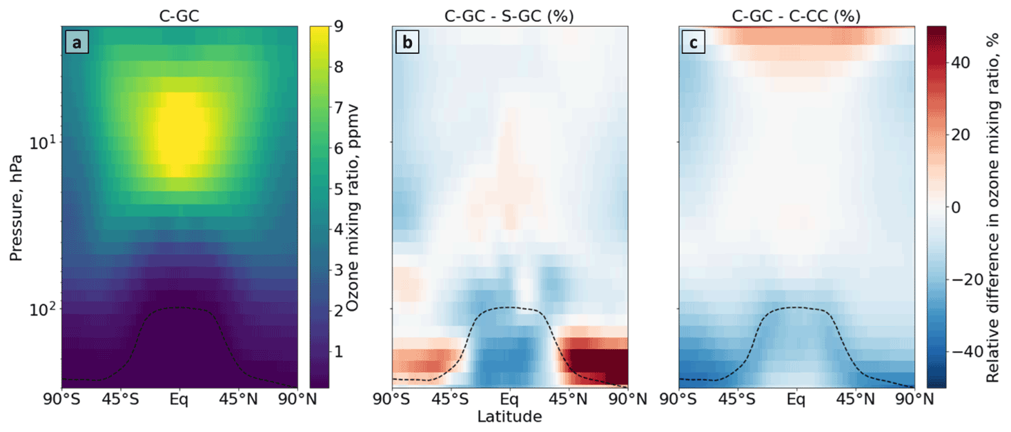
Figure 2 Comparison of stratospheric ozone simulated using CESM running GEOS-Chem (C-GC) with that simulated using the stand-alone GEOS-Chem (S-GC) and using CESM running CAM-chem (C-CC). Panel (a) presents the absolute values estimated with C-GC, panel (b) shows the relative difference between C-GC and S-GC, and panel (c) presents the relative difference between C-GC and C-CC. Red (blue) shading means that C-GC estimated a higher (lower) value than the other model. Plots show 300 to 1.65 hPa (with the latter value being the C-GC and C-CC model top).

4.1 Ozone

Figure 2 shows the annual mean mixing ratio of stratospheric ozone simulated by each of the three model configurations. At 10 hPa in the tropics, where ozone mixing ratios reach their peak, the three configurations agree to within 10 %, suggesting a reasonable representation of stratospheric ozone. However, the three configurations diverge near the tropopause. Comparison of C-GC and S-GC (Fig. 2b) shows mixing ratios 20 % lower near the tropical tropopause but more than 50 % greater in the extratropical lower stratosphere. However, C-GC simulates mixing ratios of ozone around the tropopause that are 20 % lower than C-CC (Fig. 2c) at all latitudes.

The difference in pattern in the comparison between C-GC, S-GC, and C-CC implies that the cause is likely to be related to factors that are common between C-GC and C-CC, such as the representation of meteorology. One such factor may be water vapor, which is treated differently between the “online” (C-GC, C-CC) and “offline” (S-GC) configurations.

To quantify and understand these differences in stratospheric ozone, we analyze concentrations of three different related compounds from the surface to the stratosphere: ozone, OH, and water vapor. OH reacts with most trace species in the atmosphere, and its high reactivity makes it the primary oxidizing species in the troposphere; thus, differences in abundance between models will affect the simulated abundances of many atmospheric pollutants (Seinfeld and Pandis, 2006). As OH is produced from water vapor and (indirectly from) ozone, these three compounds can collectively be used to understand some of the differences among C-GC, S-GC, and C-CC. Later analyses will focus on NO_x, bromine, and chlorine, each of which also strongly affects tropospheric and stratospheric concentrations of ozone.

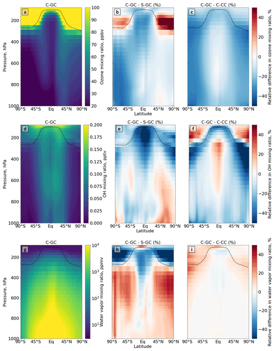
Figure 3 Comparison of the atmospheric composition simulated using CESM running GEOS-Chem (C-GC) with that simulated using the stand-alone GEOS-Chem (S-GC) and using CESM running CAM-chem (C-CC). Different rows show different constituents: ozone (a–c), OH radical (d–f), and water vapor (g–i). Different columns show different model results: the absolute values estimated with C-GC (a, d, g), the relative difference between C-GC and S-GC (b, e, h), and the relative difference between C-GC and C-CC (c, f, i). Red (blue) shading means that C-GC estimated a higher (lower) value than the other model. Plots show the surface to 100 hPa.

Figure 3a–c show the distribution of ozone as represented by C-GC (Fig. 3a) as well as the difference when compared to S-GC (Fig. 3b) or C-CC (Fig. 3c). In comparison with C-CC, C-GC estimates mixing ratios of ozone which are 30 % lower from the surface (across all latitudes) and throughout the extratropical troposphere. This is consistent with previous work which showed that tropospheric ozone simulated by GEOS-Chem to match the Korea–United States Air Quality (KORUS-AQ) campaign had a normalized mean bias of −26 %, compared with −9 % in CAM-chem (Park et al., 2021). In the present study, we find that ozone mixing ratios around the tropopause are also lower in C-GC than in C-CC (by 15 %–20 %). This suggests that discrepancies observed in KORUS-AQ may be related to chemistry rather than the treatment of meteorology, but a more focused regional analysis would be needed to confirm this.

A comparison of C-GC and S-GC provides some insight into possible causes for these discrepancies. Near-surface ozone in C-GC in the Southern Hemisphere is also 30 %–40 % lower than in S-GC, suggesting a potential common cause for the differences with C-CC. However, in the Northern extratropical troposphere below 400 hPa, zonal mean differences between C-GC and S-GC are consistently less than 10 %. Ozone concentrations are also lower in the tropical mid-troposphere in C-GC than in S-GC (by 15 %–25 %), whereas concentrations are well matched in this region between C-GC and C-CC. In the lower stratosphere, ozone concentrations in C-GC are instead greater than in S-GC, with the difference in the Northern extratropical lower stratosphere exceeding 50 %. The global ozone burden in C-GC is within 1.5 % of that estimated by S-GC, while C-CC has a total atmospheric ozone burden 15 % greater than C-GC. These model differences are evaluated against observations in Sect. 5.2.

There is a clear link between the ozone distributions and water vapor. Outside of the tropics and below the tropopause, water vapor concentrations are up to 30 % greater in C-GC than in S-GC (Fig. 3i). Differences are smaller in the tropics; however, in the tropical upper troposphere, water vapor concentrations are instead 15 % lower in C-GC than in S-GC. This may be part of the reason that water vapor concentrations in the extratropical lower stratosphere are more than 50 % lower in C-GC than in S-GC, as the tropical upper troposphere is the source of water vapor to the stratosphere. This is the same region in which C-GC calculates ozone mixing ratios that are more than 50 % greater than in S-GC, potentially due to the lower concentration of water vapor (an indirect sink of ozone). While ozone concentrations are uniformly lower for C-GC than for C-CC (Fig. 3c), water vapor concentrations differ only in the stratosphere and uppermost troposphere, where they are uniformly greater for C-GC than for C-CC (Fig. 3d).

The agreement in water vapor between C-GC and C-CC is not surprising, as the representations of transport and tropospheric moist physics in the two models are identical. Differences between S-GC and C-CC arise due to the different representation of moist processes between CAM's physics package (used in both C-GC and C-CC) and GEOS, which produces MERRA-2 and is therefore represented in S-GC. For example, although total annual average precipitation agrees to within 10 % between the models, the mean volumetric cloud fraction in C-GC and C-CC is 15 %, compared with 8 % in S-GC. Meanwhile the area-averaged cloud water content and cloud ice content are 57 % and 38 % greater, respectively, in S-GC than in C-GC (or C-CC).

Differences in ozone and water vapor result in differences in the concentrations of OH, as shown in Fig. 3d–f. The global OH atmospheric burden is approximately 10 % lower in C-GC than in S-GC (Fig. 3e), but this difference is not evenly distributed. Differences in OH concentrations can be roughly considered to be the product of differences in ozone and differences in water vapor, as both are needed to create OH (along with UV radiation). In the tropical troposphere, OH concentrations are more than 50 % lower in C-GC than in S-GC, likely due to a relative lack of both ozone and water vapor. However, in the Northern middle and upper latitudes below 900 hPa, OH concentrations are 10 %–20 % greater in C-GC than in S-GC. This reflects the greater water vapor concentrations and roughly equal ozone concentrations between the two models.

The relationship between differences in ozone and differences in water vapor is unlikely to be driven by HO_x catalytic cycles depleting ozone, as OH near the tropopause is lower in C-GC than in S-GC (Fig. 3e), and HO_x cycles are, in any case, a minor contributor to ozone depletion in the lower stratosphere (Brasseur and Solomon, 2006). The greater water vapor (and therefore humidity) may instead result in faster heterogeneous chemistry, including the liberation of NO_x from HNO₃. Differences in ozone related to tropospheric NO_y and halogens are explored in Sect. 4.4.

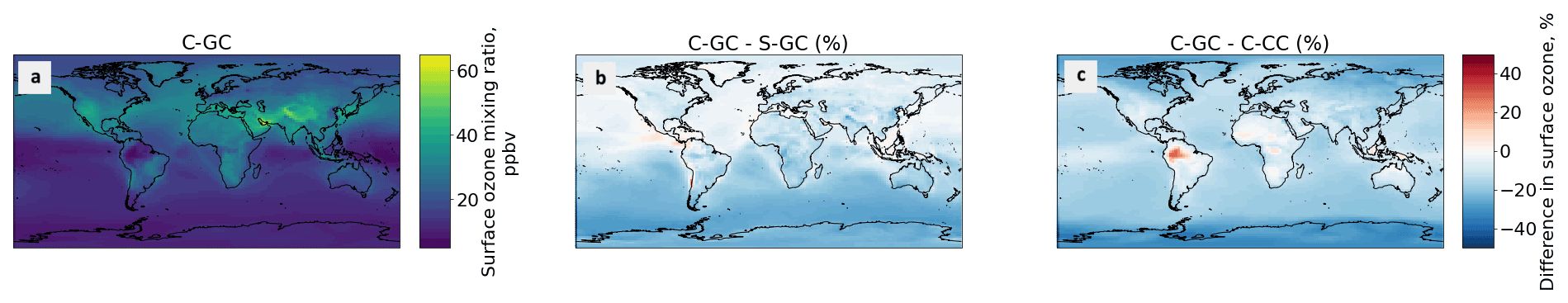
Figure 4 Comparison of the annually averaged surface ozone mixing ratios simulated using CESM running GEOS-Chem (C-GC, a) with that simulated using the stand-alone GEOS-Chem (S-GC, b) and using CESM running CAM-chem (C-CC, c). Red (blue) shading means that C-GC estimated a higher (lower) value than the other model.

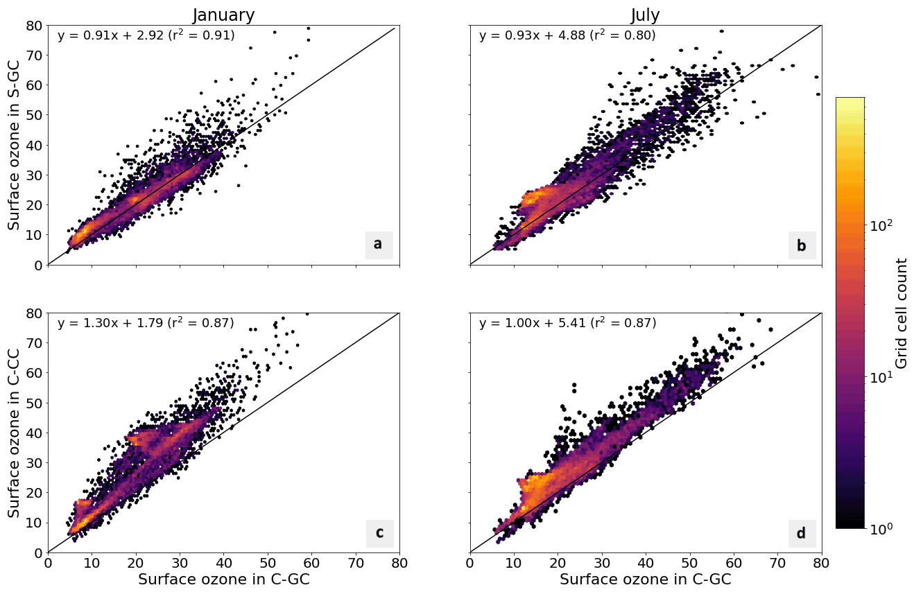
Figure 5 Parity plots of surface ozone mixing ratios, expressed in parts per billion by volume (ppbv), for January (left) and July (right) comparing C-GC on the x axis with S-GC (top) and C-CC (bottom) on the y axis. Fitting parameters are shown in the top left corner for both months. All panels share the same color scale.

4.2 Surface ozone

Figure 4 compares the simulated, annually averaged surface ozone mixing ratios as estimated by C-GC, S-GC, and C-CC. We find that, when globally averaged, C-GC predicts a lower surface ozone mixing ratio than either C-CC or S-GC. Averaged over each hemisphere, C-GC estimates a lower surface ozone mixing ratio than S-GC (Fig. 4b), by 4.9 and 2.2 ppbv in the Southern Hemisphere and Northern Hemisphere, respectively. This varies between the land and oceans. In the Northern Hemisphere, we observe a small difference in the surface ozone mixing ratio over the oceans (less than 1 ppbv), while a difference of approximately 3 ppbv can be found over North America, Europe, and East Asia.

The comparison between C-GC and C-CC (Fig. 4c) shows a similar difference in Southern Hemisphere ozone over oceans, but the relative difference now also extends to Northern Hemisphere oceans. There is also a larger difference over oceans than over land. We find that C-GC estimates  5.4 and 7.9 ppbv less ozone than C-CC in the Southern and Northern hemispheres, respectively. The pattern indicated in Fig. 4c suggests that bromine from sea salt may be the principal cause of the differences in surface ozone between C-GC and C-CC, whereas differences between C-GC and S-GC are likely to be related to anthropogenic emissions given the hemispheric asymmetry. The 20 %–30 % increase in ozone over the Amazon in C-GC related to C-CC may instead be related to differences in biogenic emissions. Differences in Northern Hemispheric ozone may be attributable to the different chemical response to anthropogenic emissions in the GEOS-Chem and CAM-chem mechanisms.

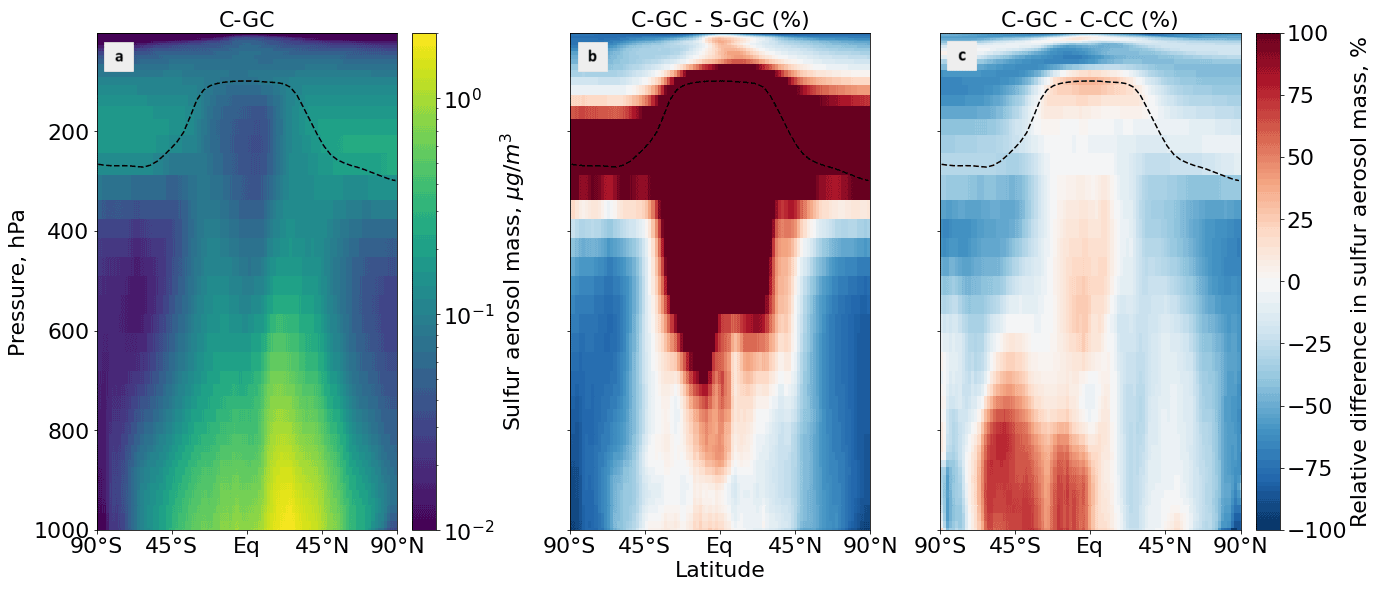
Figure 6 Comparison of the sulfate aerosol mass concentration as simulated using CESM running GEOS-Chem (C-GC) with that simulated using the stand-alone GEOS-Chem (S-GC) and using CESM running CAM-chem (C-CC). Panel (a) presents the absolute values estimated with C-GC, panel (b) shows the relative difference between C-GC and S-GC, and panel (c) presents the relative difference between C-GC and C-CC. Red (blue) shading means that C-GC estimated a higher (lower) value than the other model. Differences are restricted to ± 100 % for clarity. Plots show the surface to 1.65 hPa (with the latter value being the C-GC and C-CC model top).

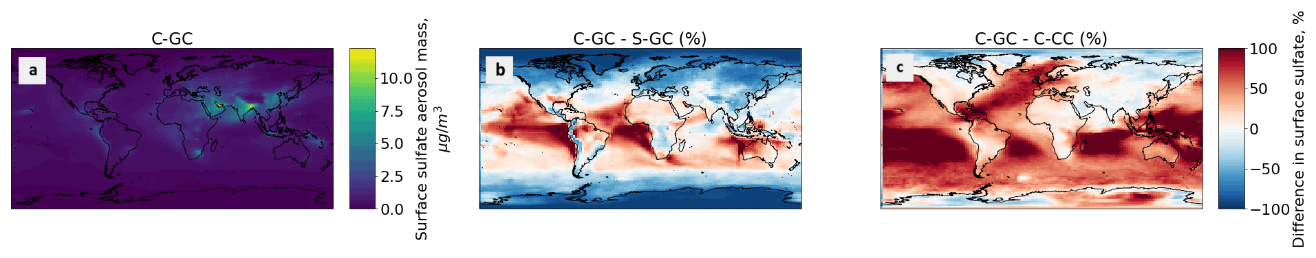
Figure 7 Comparison of the annually averaged surface mass concentration of sulfate aerosol simulated using CESM running GEOS-Chem (C-GC) with that simulated using the stand-alone GEOS-Chem (S-GC) and using CESM running CAM-chem (C-CC). Red (blue) shading means that C-GC estimated a higher (lower) value than the other model.

In addition to annual averages, we also consider seasonal variations in surface ozone. Figure 5 presents parity plots of monthly averaged surface ozone mixing ratios for January and July comparing C-GC to S-GC and C-CC, after outputs from all three model configurations were remapped to a common 2^∘ × 2.5^∘ grid. In January, we find a correlation coefficient of 0.91 and a slope of 0.91 between C-GC and S-GC. In July, this agreement is worsened, with a correlation coefficient of 0.80 but a slope of 0.93. This indicates that the sources of differences in surface ozone mixing ratios between C-GC and S-GC are magnified during boreal summer. There is also a distinctive “hot spot” in the July parity plot, with a large cluster of grid cells showing mixing ratios in the 20–25 ppbv range in both S-GC and C-CC but in the 10–20 ppbv range in C-GC. Further research is needed to establish the origin of this cluster, which does not occur during boreal winter, in addition to other disagreements such as a patch of grid cells at around 40 ppbv in January in C-CC which are at around 20 ppbv in C-GC.

Comparison between C-GC and C-CC shows a different pattern. The line of best fit between C-CC and C-GC indicates 30 % greater ozone in C-CC in January than in C-GC (y ∼ 1.3×), but no such normalized mean bias is present in July (y ∼ 1.0×). As with the comparison of C-GC to S-GC, the absolute bias is greater in July than in January, but the correlation between C-CC and C-GC does not worsen between the 2 months (r² = 0.87). This may indicate the strength of the effect of meteorology and non-chemistry processes in the seasonality of simulated surface ozone.

4.3 Aerosols

Figure 6 shows the zonal mean mass concentration of sulfate aerosol as simulated in each of the three model configurations. In C-GC and C-CC, this is calculated as the sum across all aerosol size bins, whereas S-GC uses a bulk representation.

Figure 8 Comparison of the primary organic matter aerosol mass concentration as simulated using CESM running GEOS-Chem (C-GC) with that simulated using the stand-alone GEOS-Chem (S-GC) and using CESM running CAM-chem (C-CC). Panel (a) presents the absolute values estimated with C-GC, panel (b) shows the relative difference between C-GC and S-GC, and panel (c) presents the relative difference between C-GC and C-CC. Red (blue) shading means that C-GC estimated a higher (lower) value than the other model. Plots show the surface to 1.65 hPa (with the latter value being the C-GC and C-CC model top).

Between 45^∘ S and 45^∘ N, and below 800 hPa, C-GC more closely follows S-GC (comparison in Fig. 6b) with regards to sulfate aerosol mass. Compared with C-CC (Fig. 6c), sulfate aerosol mass is approximately 50 % greater in Southern latitudes, with differences being greatest over the oceans (see Fig. 7). Sulfate concentrations in this region are dominated by the oxidation of naturally emitted dimethyl sulfide (DMS) (Seinfeld and Pandis, 2006). As DMS concentrations are identical between the three configurations, the greater sulfate concentration in C-GC compared with C-CC may instead reflect differences in OH (Fig. 3) and different approaches to in-cloud sulfur chemistry (see Sect. 2.3.1). Elsewhere, the concentration of sulfate in C-GC more closely follows that in C-CC (differences of ± 25 %; Fig. 6c). This is likely due to the common representation of sulfate aerosol in MAM4 and differences in the representation of convective scavenging between CESM and the stand-alone GEOS-Chem model. Concentrations of sulfate in the tropical mid-to-upper troposphere and extratropical lower stratosphere in C-GC exceed those in S-GC by over 100 % (Fig. 6b).

This is further illustrated in Fig. 7, which shows the surface concentration of sulfate aerosol in each model configuration. C-GC simulated greater concentrations in the Intertropical Convergence Zone (off the west coast of Southern Hemisphere continents) than in S-GC (Fig. 7b), but it agrees more closely with C-CC in these regions (Fig. 7c). Elsewhere in the tropics, the agreement between C-GC and S-GC is stronger, whereas surface concentrations of sulfate aerosol over (e.g.) the southern Pacific exceed those in C-CC by over 100 %. At high latitudes and over land, the agreement between C-GC and C-CC is again stronger than in S-GC, although this varies by location. Further work would be needed to identify the underlying causes leading to differences in surface sulfate concentrations between all three models.

We also show the zonal mean concentrations of primary organic matter (POM) aerosol in each configuration (Fig. 8). POM in C-GC and C-CC is calculated as the sum of the POM aerosol size bins, whereas it is calculated as the sum of the hydrophobic and hydrophilic organic carbon species in S-GC. As with sulfate aerosol, C-GC and S-GC agree to within 25 %–50 % in the tropics below 800 hPa, but C-GC simulates concentrations of POM that are over 100 % greater than S-GC in the middle and upper tropical troposphere and throughout the lower stratosphere. This is again likely due to differences in the representation of convective scavenging. C-GC also simulates concentrations of POM that are lower than C-CC throughout the entire troposphere. This is likely due to differences in the implementation of POM emissions between C-CC and C-GC. Although emissions of POM in C-CC are 29 % lower, they occur as accumulation-mode rather than primary-organic-mode aerosol, which may extend their lifetime.

4.4 Reactive nitrogen (NO_y), bromine (Br_y), and chlorine (Cl_y)

To better understand the source of differences in ozone and aerosols described above, we now investigate differences in the reactive nitrogen (NO_y) and halogen families. Halogens are involved in multiple catalytic ozone-depleting chemical cycles, and they are critical to an accurate description of both tropospheric and stratospheric chemistry (Solomon et al., 2015). Therefore, we analyze the abundance and speciation of two key halogen families – bromine (Br_y) and chlorine (Cl_y) – in each configuration.

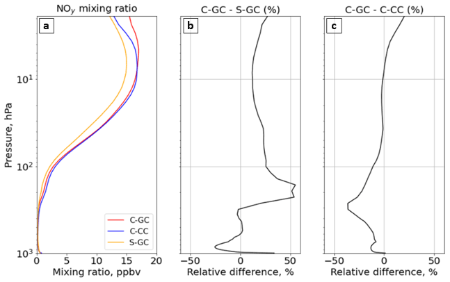
Figure 9 The global annual mean mixing ratio of total reactive nitrogen (NO_y) as a function of altitude. Panel (a) presents the profile of the NO_y mixing ratio for C-GC (red), C-CC (blue), and S-GC (orange); panel (b) shows the relative difference in the NO_y mixing ratio between C-GC and S-GC; and panel (c) presents the relative difference in the NO_y mixing ratio between C-GC and C-CC. Plots show the surface to 1.65 hPa (with the latter value being the C-GC and C-CC model top).

4.4.1 Reactive nitrogen (NO_y)

We compare the total concentration and partitioning of reactive nitrogen species in each model configuration, including NO_x and its reservoir species (collectively NO_y). A full list of the species included in the lumped NO_y reservoir species can be found in the legend of Fig. 10 for each model configuration. We first compare results in the stratosphere, followed by an evaluation of concentrations and partitioning below 100 hPa. Concentrations of nitrate aerosol concentrations are estimated in CAM-chem using a simplified approximation (Lamarque et al., 2012), and particulate nitrate is typically not considered to be simulated by CAM-chem (e.g., Park et al., 2021). Therefore, we do not include it in this analysis.

Figure 9 shows global mean NO_y at each altitude for C-GC, C-CC, and S-GC. Comparing C-GC to S-GC (Fig. 9b), differences in total NO_y are within −26 to +55 % at all altitudes. Between 100 and 10 hPa, C-GC differs from S-GC by less than 20 %, compared to less than 10 % with respect to C-CC (Fig. 9c). The difference between C-GC and C-CC increases from −2 % at 10 hPa to +20 % at the top of the model, compared to an increase from 10 % to 25 % when comparing C-GC to S-GC. At lower altitudes, C-GC more closely follows C-CC than S-GC, with differences between C-GC and S-GC exceeding 50 % between 200 and 300 hPa. The global NO_y burden in C-GC (2.74 Tg(N)) is closer to that in S-GC (2.84 Tg(N)) than that in C-CC (3.01 Tg(N)), likely due to the stronger influence of the troposphere on this quantity.

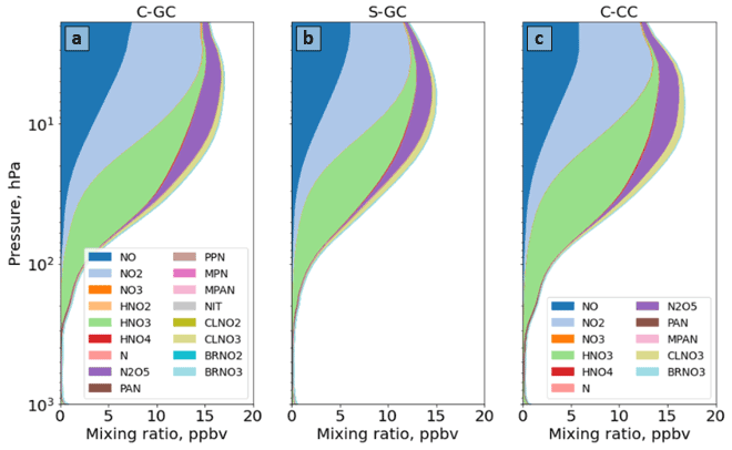
Figure 10 The global annual mean speciation of NO_y as a function of altitude. Results are shown from C-GC (a), S-GC (b), and C-CC (c) from the surface up to the model top (1.65 hPa). Values correspond to the number of N atoms present, such that, for example, the mixing ratio of N₂O₅ is multiplied by 2. For more information on the species listed in the figure legends, the reader is referred to http://wiki.seas.harvard.edu/geos-chem/index.php/Species_in_GEOS-Chem (last access: 24 November 2022).

Figure 10 shows the speciation of NO_y as a function of altitude in each model from the surface to 1 hPa. The list of species defined collectively as NO_y differs between C-GC and S-GC on one side and C-CC on the other side. At altitudes above 100 hPa, the dominant contributors to NO_y in all three model configurations are NO, NO₂, HNO₃, and N₂O₅, although ClNO₃ contributes significantly between approximately 80 and 5 hPa. Between 10 and 200 hPa, NO:NO₂ ratios are approximately consistent between the models, lying in the range from 0.35 to 0.50. This suggests broad consistency in actinic flux and ozone concentrations, given their role in controlling NO:NO₂ ratios in the stratosphere (Cohen and Murphy, 2003).

Whereas total NO_y up to 10 hPa appears to be more consistent between the two configurations operating within CESM (C-CC and C-GC), partitioning appears to be more consistent between the two configurations using GEOS-Chem chemistry (C-GC and S-GC). At 10 hPa, HNO₃ constitutes 20 % of total NO_y in C-GC but 23 % in both C-CC and S-GC (values not shown explicitly). This fraction increases with decreasing altitude at differing rates. At 200 hPa, HNO₃ constitutes 60 % and 63 % of NO_y in C-GC and S-GC, respectively, but 78 % of NO_y in C-CC. One possible cause of these discrepancies is heterogeneous chemistry. GEOS-Chem (in both S-GC and C-GC) uses a different representation of N₂O₅ hydrolysis than CAM-chem, but the CESM-driven simulation includes a more detailed representation of the sulfate aerosol size distribution through MAM4 and shows different sulfate aerosol mass concentrations in the troposphere (Fig. 6). The present study did not include the analysis of aerosol reactive tendencies. This would be a valuable line of inquiry for future comparisons of CAM-chem and GEOS-Chem, given the lack of nitrate aerosol in the former.

Figure 11 As in Fig. 10 but showing only the 10³–10² hPa pressure range.

Figure 11 provides a closer look at the speciation of NO_y at altitudes below 100 hPa. NO_y at altitudes below 200 hPa is predominantly NO_x, HNO₃, and peroxyacetyl nitrate (PAN). At 200 hPa, the same combination of species (NO_x, HNO₃, and PAN) makes up 86 % of total NO_y in C-GC (Fig. 11a) and 84 % in S-GC (Fig. 11b), but these species only account for 96 % of total NO_y in C-CC (Fig. 11c). However, the dominant contributors are HNO₃ and PAN between 200 and 900 hPa. In this pressure range, the C-GC and S-GC simulations also show a significant contribution from nitrate aerosol (NIT) and BrNO₃. At 500 hPa, the contributions of NO_x, HNO₃, and PAN are 78 %, 85 %, and 97 %, respectively, for C-GC, S-GC, and C-CC. Below 900 hPa, NO and NO₂ once again become significant contributors to total NO_y.

As surface emissions of NO_x are nearly identical between the three configurations (see Table 2) and lightning NO_x emissions are calculated using the same parameterization in both C-GC and C-CC, differences below 100 hPa may instead be related to NO_x chemistry and nitrate aerosol. However, concentrations of PAN in C-GC more closely follow C-CC than S-GC, suggesting that the representation of meteorology (including wet-deposition rates) is also an important factor. At 500 hPa, total PAN in C-GC is 3 % lower than the value in C-CC but exceeds the value in S-GC by 38 %. This may be due to the greater emissions of biogenic VOCs in CESM than in the stand-alone GEOS-Chem model (see Table 3), resulting in more NO_x being bound into PAN for long-range transport. We also find that HNO₃ concentrations in the mid-troposphere are lower in C-GC than in either C-CC or S-GC. At 500 hPa, HNO₃ mixing ratios in C-GC are 43 % lower than in S-GC and 52 % lower than in C-CC. This does not account for the conversion of HNO₃ to nitrate aerosol (NIT) in C-GC and S-GC, which is not represented in C-CC. The ratio of nitrate in aerosol compared to that in gaseous HNO₃ is similar at low altitudes (below 900 hPa) between C-GC and S-GC, with nitrate mixing ratios being lower than HNO₃ at 900 hPa but greater than HNO₃ at the surface.

Differences in mid-tropospheric HNO₃ between the models are most likely due to differences in the representation of wet scavenging. In C-CC and C-GC, scavenging of gaseous species is handled by the Neu scheme (Neu and Prather, 2012), whereas scavenging of modal aerosols is performed by MAM. Any aerosol species not handled by MAM, such as nitrate in C-GC, are also scavenged using the Neu scheme. In C-GC and C-CC, the Neu scheme calculations are performed at the same time as the chemistry and after convective transport, whereas scavenging of MAM aerosols is performed before. Thus, all species that undergo wet deposition in the Neu scheme are not removed during convective transport. This leads to soluble species and aerosols being carried to higher altitudes without being convectively scavenged. We also find that the Neu scavenging scheme in C-GC and C-CC results in an HNO₃ wet removal rate that is 4 times higher in C-GC than in S-GC (Fig. S1 in the Supplement). This likely explains the greater depletion of HNO₃ in the mid-troposphere calculated by C-GC compared with S-GC. Wet scavenging in C-CC is even faster, with HNO₃ wet-removal rates approximately 6 times greater than in S-GC and 50 % greater than in C-GC. This is in part because the mixing ratio (or fraction of total NO_y) of HNO₃ in the middle and upper troposphere as modeled in C-CC is greater than in either C-GC or S-GC but also because C-GC and S-GC simulate nitrate aerosol explicitly. The application of the Neu scheme to remove nitrate aerosol also affects the removal of total NO_y in C-GC (Fig. S2 in the Supplement). We find that the Neu scheme removes aerosol more rapidly than the scheme used in S-GC (Liu et al., 2001) as well as at lower altitudes.

Total HNO₃ removal tendencies in each model configuration are shown in Table 7. The total removal rate of ${\mathrm{NO}}_{\mathrm{3}}^{-}$ is lowest in S-GC and highest in C-CC, consistent with the finding that total NO_y burdens are lower in S-GC than in C-GC or C-CC. However, the removal rate of nitrate aerosol is lower in C-GC than in S-GC despite the greater wet-removal rates for C-GC. A possible explanation for this is that washout rates of nitrate aerosol are sufficiently high in both C-GC and S-GC that all nitrate aerosol is effectively removed, but the faster washout of HNO₃ in C-GC results in less nitrate aerosol being available for removal.

Table 7 The total wet-removal tendency of HNO₃ and nitrate aerosol in each model configuration. All values are given in teragrams of nitrate per year (Tg NO₃ yr⁻¹).

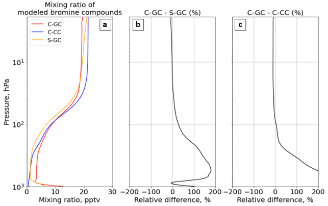
Figure 12 The global annual mean mixing ratio of reactive bromine as a function of altitude. Panel (a) presents the profile of the total gaseous inorganic and organic bromine mixing ratio for C-GC (red), C-CC (blue), and S-GC (orange); panel (b) shows the relative difference in the bromine-containing species mixing ratio between C-GC and S-GC; and panel (c) presents the relative difference in the bromine-containing species mixing ratio between C-GC and C-CC. Although relative differences between C-GC and C-CC exceed 1000 % near the surface, the limits on the panel (c) are clipped to allow comparison to panel (b). Plots show the surface to 1.65 hPa (with the latter value being the C-GC and C-CC model top).

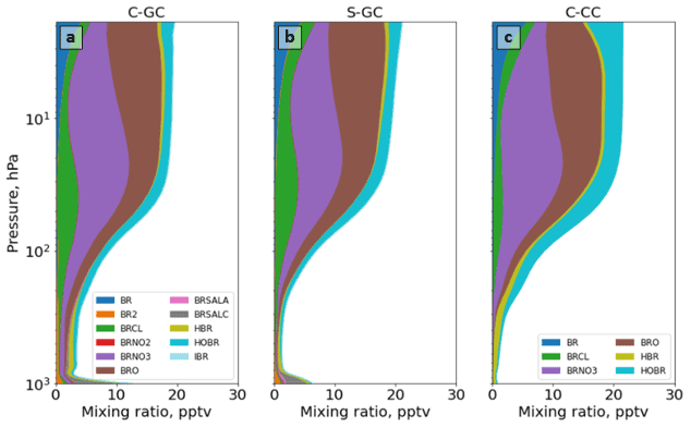
Figure 13 The global annual mean speciation of total organic and inorganic bromine as a function of altitude. Results are shown from C-GC (a), S-GC (b), and C-CC (c) from the surface up to the model top (1.65 hPa). Values correspond to the number of Br atoms present, such that, for example, the mixing ratio of Br₂ is multiplied by 2.

4.4.2 Reactive bromine (Br_y)

Figure 12 shows the annual average mixing ratio of total reactive bromine as a function of altitude in each of the three models. This does not include long-lived species such as halons or CH₃Br. A full listing is included in the legend of Fig. 13.

Globally averaged total Br_y in C-GC is maximized at the surface, where it is double that of S-GC (Fig. 12b). This is partially explained by the greater emissions of sea-salt bromine, although C-GC's annual emission of sea-salt bromine is only 36 % greater than that in S-GC (see Table 4). As C-CC does not include short-lived bromine sources such as sea-salt bromine, the C-GC total Br_y concentration exceeds C-CC by 1000 % at the surface (Fig. 12c). In all three models, the mixing ratio increases monotonically with altitude above 800 hPa, before stabilizing at around 50 hPa. The increase with altitude is due to the reaction of CH₃Br with OH and is, therefore, a function of both CH₃Br emissions and the distribution of OH, which varies between models (see Fig. 3).

Figure 13 shows Br_y partitioning across all three models. Br_y falls sharply from 12 pptv at the surface in C-GC to 3 pptv at 900 hPa, but it then increases again to 10 pptv at 100 hPa. This pattern is similar to that displayed by S-GC, although the decrease from the surface is less sharp and the absolute value is lower in S-GC. Above 100 hPa, the averaged Br_y mixing ratio levels off, with values between 20 hPa and 2 hPa remaining roughly constant in the range of 16–20 pptv. This is similar to the behavior shown by C-CC but differs from S-GC, in which Br_y continues to rise with altitude – albeit more slowly. The net effect is that total Br_y in C-GC exceeds both C-CC and S-GC below 100 hPa, but it is lower than the value in either model above 10 hPa (above 80 hPa when compared to C-CC).

In addition to differences in total Br_y, the partitioning of Br_y also varies between the three models (Fig. 13). The additional near-surface bromine present in C-GC and S-GC is due to the presence of Br₂ and sea-salt bromine (BrSALA and BrSALC, representing bromine in fine- and coarse-mode sea salt, respectively). This provides a source of active bromine in the planetary boundary layer, which is not represented in C-CC, but in forms that are rapidly washed out in C-GC and S-GC. The greater concentrations of Br_y near the surface as calculated by C-GC compared with S-GC are likely due to the greater emissions of sea-salt bromine, as shown in Table 4.

Br_y in the model stratosphere is dominated by the same species in all three configurations: BrO_x (Br + BrO), BrCl, BrNO₃, HBr, and HOBr. The most significant difference is the greater proportion of HOBr in C-CC (approximately 15 %) than in S-GC or C-GC (8 %–10 %). Larger mixing ratios of BrNO₃ are also present in C-CC (approximately 10 ppbv at 30 hPa) compared with C-GC and S-GC (approximately 7.4 and 7.0 ppbv at 30 hPa, respectively). Smaller mixing ratios of BrCl are present in C-CC, with a mean value of 1.8 ppbv at 30 hPa, whereas they reach 3.1 ppbv in C-GC and S-GC at 30 hPa. The base causes of these differences are not clear, but they may be related to the presence of more complex tropospheric and stratospheric halogen chemistry in the GEOS-Chem chemical mechanism (Wang et al., 2021).

Between 30 hPa and the top of the boundary layer, the three models show greater divergence. The only significant sources of atmospheric Br_y in C-CC are CH₃Br, CH₂Br₂, and very long-lived bromine species such as halons which are insoluble. As a result, tropospheric Br_y concentrations increase only slowly from the surface up to 300 hPa, at which point HOBr, BrO, and BrNO₃ begin to form in significant quantities. In C-GC and S-GC, these sources of bromine are supplemented by bromine from sea-salt and surface Br₂ emissions. Mid-tropospheric Br_y concentrations are, therefore, largely set by the quantity of sea-salt bromine emitted and by the fraction of that bromine which can be released to an insoluble form (e.g., Br₂) before the sea salt is washed out of the atmosphere.

The greater concentration of mid-tropospheric Br_y in C-GC than in S-GC (exceeding a 100 % difference, as shown in Fig. 12b) is likely due to differences in wet scavenging. Wet-removal tendencies of bromine in fine sea salt (BrSALA) from large-scale and convective precipitation as calculated by C-GC and S-GC are shown in the Supplement (Fig. S3). We find that there is greater wet deposition of fine-sea-salt bromine in S-GC than in C-GC, despite removal rates below 900 hPa being greater in C-GC. As total emissions of BrSALA are also 26 % lower in S-GC than in C-GC (Table 4), the slower mid-tropospheric removal of bromine in C-GC explains the greater simulated concentration of Br_y.

C-GC also calculates wet deposition of non-MAM aerosols from both convective and large-scale precipitation independent of convective transport, whereas S-GC calculates convective scavenging as part of convective transport. This means that soluble species can be transported in convective updrafts in C-GC, unlike in S-GC.

Figure 14 Comparison of the annual average vertical profiles of chlorine-containing compounds in the three models. Panel (a) presents the vertical profile of the total gaseous chlorine mixing ratio for C-GC (red), S-GC (orange), and C-CC (blue); panel (b) shows the relative difference in the Cl_y mixing ratio between C-GC and S-GC; and panel (c) presents the relative difference in the Cl_y mixing ratio between C-GC and C-CC. Although the relative differences between C-GC and C-CC exceed 1000 % near the surface, the limits on panel (c) are clipped to allow comparison to panel (b). Plots show the surface to 1.65 hPa (with the latter value being the C-GC and C-CC model top).

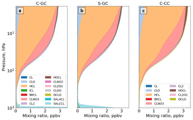
Figure 15 The global annual mean vertical speciation of total organic and inorganic bromine in C-GC (a), S-GC (b), and C-CC (c) from the surface up to the model top (1.65 hPa). Values correspond to the number of Cl atoms present, such that, for example, the mixing ratio of Cl₂ is multiplied by 2. SALACL and SALCCL correspond to chlorine in fine and coarse sea salt, respectively.

4.4.3 Reactive chlorine (Cl_y)

We now focus on atmospheric chlorine by comparing its profile and partitioning in all three models. Annually averaged profiles of Cl_y are displayed in Fig. 14, excluding source species such as chlorocarbons. A full list of the species used to define Cl_y in each configuration is provided in Fig. 15.

Comparing C-GC to S-GC (Fig. 14b), differences in total Cl_y follow a similar pattern to Br_y (Fig. 12b) up to 10 hPa. At the surface, the greater sea-salt chlorine in C-GC relative to S-GC results in differences exceeding 100 %. In comparison to C-CC (Fig. 12c), the dominant factor in differences below 100 hPa is the lack of short-lived chlorine species such as sea salt in C-CC, which are the dominant source of chlorine to the lower troposphere. Above 10 hPa, the relative difference in Cl_y between C-GC and S-GC increases slowly from −2 % at 10 hPa to −5 % at 2 hPa, while the difference relative to C-CC remains at approximately −20 % above 200 hPa.

Figure 15 shows the speciation of Cl_y as a function of altitude in each model. The greater near-surface chlorine simulated by C-GC (Fig. 15a) and S-GC (Fig. 15b) relative to C-CC (Fig. 15c) is mostly made up of HCl and chlorine in sea salt (SALACL and SALCCL). However, the short lifetime of sea-salt aerosol and of chlorine in the lower troposphere means that this source is likely not significantly affecting stratospheric chlorine burdens or partitioning. In the stratosphere, there is no clear difference between partitioning in C-GC and S-GC, but larger mixing ratios of upper-tropospheric and lower-stratospheric HCl (specifically, between 200 and 50 hPa) from chlorine source compounds are found in C-CC. At 50 hPa, total Cl_y in C-CC is 15 % greater than in C-GC and S-GC (see Fig. 14a), but the mean mixing ratio of HCl in C-CC is 45 % greater. Differences in ClNO₃ reach their peak at higher altitudes, around 20–30 hPa.

The global mean tropospheric concentration in of Cl atoms in C-GC is 590 cm⁻³, roughly consistent with a recent evaluation from Wang et al. (2021) that found a value of 630 cm⁻³. This is 24 % greater than the value from S-GC (477 cm⁻³) and 160 % greater than that from C-CC (224 cm⁻³), likely due to the greater emissions of sea salt and indicating that chlorine will play a greater role in tropospheric oxidation in C-GC.

5 Comparison of model results to observations

We now compare the results from C-GC to observational data, with results from S-GC and C-CC also provided for context. Section 5.1 evaluates model performance at the surface, providing a comparison to ground measurements of surface NO₂ and ozone. Section 5.2 compares model results to a climatology of vertical profiles of ozone, based on ozonesonde data. Section 5.3 evaluates the level of agreement of simulated ozone and carbon monoxide (CO) columns to measurements from the Aura OMI and Microwave Limb Sounder (MLS) as well as the Terra Measurement of Pollution in the Troposphere (MOPITT) satellite instruments. Finally, Sect. 5.4 evaluates the model against measurements of dry-deposition fluxes and rainwater composition measurements. The CESM wet-deposition scheme is presented in Neu and Prather (2012), whereas the wet-deposition scheme implemented in GEOS-Chem uses different schemes for gases and aerosols (Liu et al., 2001; Amos et al., 2012). Dry deposition in GEOS-Chem has been described in several publications (Wesely, 1989; Wang et al., 1998; Zhang et al., 2001), and the coupling between CAM and CLM is described in Val Martin et al. (2014).

Figure 16 Annual average surface NO₂ mass concentrations simulated by C-GC (a, e, h), S-GC (b, f, i), and C-CC (c, g, j) for 2016 compared against monitor measurements in North America (a–c), Europe (d–e), and Southeast Asia (h–j).

5.1 Surface NO₂ and ozone

Figure 16 compares surface mass concentrations of NO₂ as estimated by C-GC, S-GC, and C-CC for 2016 against ground station measurements for North America (panels a–c), Europe (panels e–g), and Southeast Asia (panels h–j) (AirNow API, 2021; Environmental Numerical Database, 2021; China Air Quality Historical Data, 2021; European Air Quality Portal, 2021). All ground station measurements are the average value over 2016. By comparing model results at an approximately 2^∘ horizontal resolution to point observations, we expect some differences in this evaluation due to grid-box representation errors.

All three model configurations calculate lower mixing ratios than are reported by the ground observations. This is likely to be in part due to the presence of interferants such as HNO₃, which cause in situ monitors to overestimate the concentration of NO₂ (Dunlea et al., 2007). However, S-GC is consistently biased lower than C-GC or C-CC. We also find that the surface NO₂ concentrations display variable agreement depending on the geographical location. The correlation coefficients for North America, Europe, and Southeast Asia are provided in Table 8. All three models give similar correlation coefficients for each region. This is expected given that the three model configurations all use the same input wind fields and NO_x emissions datasets. Nonetheless, both C-GC and C-CC estimate higher concentrations of NO₂ in northern China, northern Europe, and the northeastern US than S-GC. This suggests that the representation of meteorology, photolysis, and NO_y removal processes have a greater impact on simulated NO₂ than the chemistry module alone. Comparing in situ NO₂ measurements against NO_y model results could potentially remove the effect of interferants in the observations of surface NO₂ concentrations, but this is not considered here.

Table 8 Correlation coefficients of surface-level NO₂ mass concentrations for C-GC, S-GC, and C-CC against measurements.

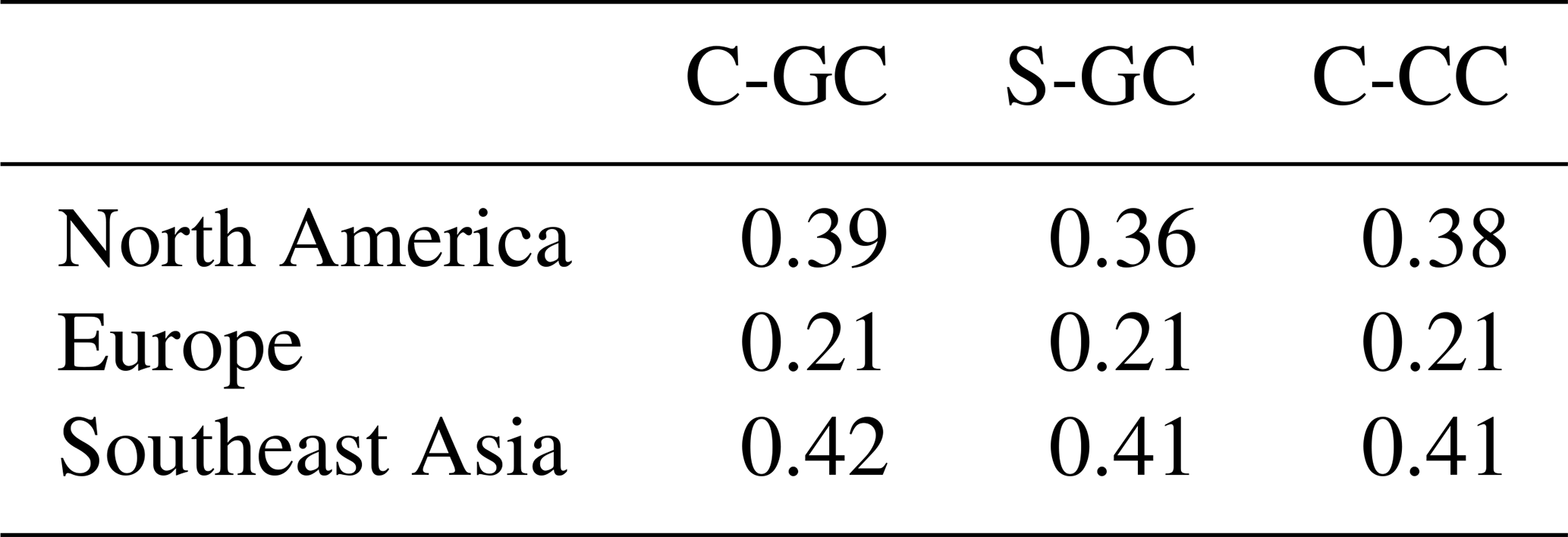
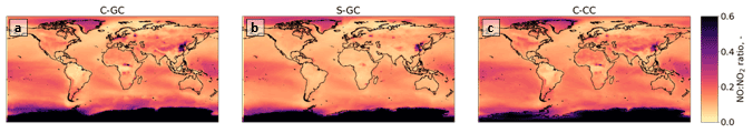
Figure 17 Surface-level NO:NO₂ ratios estimated by C-GC (a), S-GC (b), and C-CC (c) for 2016. The annual average of NO:NO₂ is calculated as the annual mean NO divided by the annual mean NO₂.

Figure 17 shows the ratio of annual mean NO to annual mean NO₂, thereby providing some insight into possible causes of these disagreements. The global distribution of surface-level NO₂ and NO_x is presented in the Supplement. All three configurations show enhanced NO:NO₂ ratios in polluted regions, such as eastern China, and over icy regions, such as Greenland and Antarctica. However, S-GC shows reduced NO:NO₂ ratios over land compared with both C-CC and C-GC. For example, ratios over North America in S-GC range from 0.1 to 0.2, compared with a range of 0.01 to 0.1 in C-GC and C-CC. Surface NO:NO₂ ratios are typically dictated by surface ozone and the NO₂ photolysis rate (Seinfeld and Pandis, 2006). Given that surface ozone concentrations in S-GC are typically between those calculated in C-GC and C-CC (see Fig. 4) and that S-GC and C-GC share the same photolysis treatment, this discrepancy may instead be caused by the differences in cloudiness calculated by CESM compared with the MERRA-2 fields read in by S-GC.

Differences in NO:NO₂ may also be related to differences in emissions and the treatment of oxidants such as VOCs and bromine. C-GC and C-CC show a reduction in NO:NO₂ over the Amazon and in the Congo River basin, but this pattern is not reproduced in S-GC. Similarly, topographical features including the Andes and Himalayas are visible in the C-CC and C-GC NO:NO₂ ratios but not in the S-GC data – whereas a large reduction in NO:NO₂ over the Arctic Ocean is more pronounced in S-GC and C-GC than in C-CC. This latter feature may be related to differences in the response of the simulated atmosphere to anthropogenic emissions, as ship tracks are more visible in the C-GC and S-GC NO:NO₂ ratios (see, e.g., Cape Horn and the Cape of Good Hope) than in C-CC.

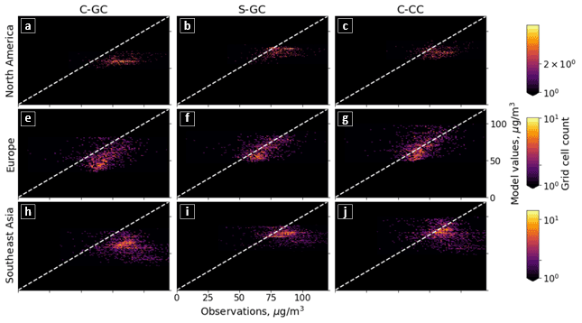
Figure 18 Annual average surface ozone mass concentrations simulated by C-GC (a, e, h), S-GC (b, f, i), and C-CC (c, g, j) for 2016 compared against monitor measurements in North America (a–c), Europe (d–e), and Southeast Asia (h–j).

Figure 18 compares surface ozone against monitor measurements, with correlation coefficients shown in Table 9.

Table 9 Correlation coefficients and mean biases in parts per billion by volume (ppbv; in parentheses) of surface-level ozone mass concentrations for C-GC, S-GC, and C-CC against measurements.

Although simulated ozone follows a broadly consistent geographical pattern (see Fig. 4), the results from all model configurations appear to be biased low. As discussed in Sect. 4.2, C-GC estimates surface ozone mixing ratios lower than either S-GC and C-CC; therefore, C-GC exhibits the greatest mean bias (shown in Table 9).

The greater negative bias in simulated ozone shown by C-GC is likely related to both the different representation of meteorology compared with S-GC and the greater bromine emissions compared with both S-GC and C-CC. However, further work is needed to disentangle the root causes of discrepancies between the three models, and the common biases relative to observations.

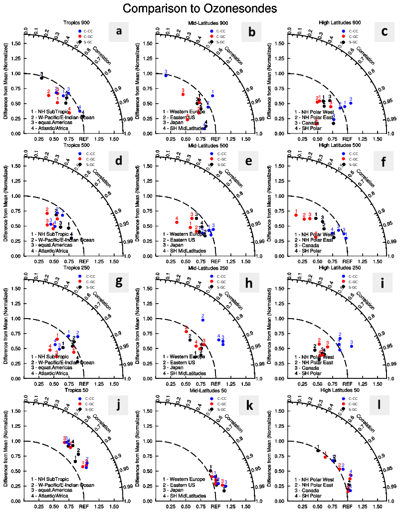
Figure 19 Taylor diagrams of the comparison of C-GC (red), C-CC (blue), and S-GC (black) simulations to a present-day (1995–2010) ozonesonde climatology. The rows show comparisons at 900 (a–c), 500 (d–f), 250 (g–i), and 50 hPa (j–l), and the columns show results for the tropics (a, d, g, j), midlatitudes (b, e, h, j), and high latitudes (c, f, i, l). The normalized mean difference between simulations and observations for each region is shown on the radius, and the correlation of the seasonal cycle is shown as the angle from the vertical.

5.2 Vertical profiles of ozone

We now focus on the evaluation of the profile of ozone mixing ratios by comparing C-GC, C-CC, and S-GC to a climatology of ozonesonde observations from 1995 to 2010 (Tilmes et al., 2012). This climatology (in addition to those shown in Sect. 5.3) has been used repeatedly in evaluations of CAM-chem; therefore, it is chosen here to provide a familiar point of comparison which also allows the three configurations to be compared to a realistic baseline. Over the past decades, observations from ozonesondes in different locations have provided a valuable dataset of the evolution of ozone mixing ratios in the troposphere and stratosphere. Figure 19 provides a Taylor diagram comparison between the C-GC, C-CC, and S-GC simulations of 2016 to the climatology.

In general, C-GC does not perform significantly better or worse than C-CC or S-GC, producing mean biases and correlations in each region–altitude combination that are within the same range. The clearest exception is at low altitudes (900 or 500 hPa) and middle to high latitudes (Fig. 19b, c, e, f). In these regions, C-GC results frequently show a smaller normalized difference from the mean (radius) than either S-GC or C-CC as well as a weaker correlation with the observed seasonal cycle. The C-GC simulation of tropical ozone also shows the smallest mean bias at all altitudes at or below 250 hPa (Fig. 19a, d, g), although again showing a weaker correlation.

At high altitude (50 hPa; Fig. 19j, k, l), all three model configurations appear to perform similarly. This may, however, simply reflect the lack of spin-up time. As the three configurations only simulated 1.5–2 years in total, the simulated stratosphere will not have had time to fully respond to the new configuration. This is evident in Fig. 2, which shows similar stratospheric ozone in all three configurations. Longer simulations are needed to fully evaluate the performance and capability of the C-GC stratosphere.

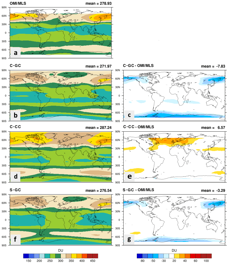
Figure 20 The total ozone column in Dobson units (DU) as observed by OMI/MLS for the 2004–2010 time period (a) compared to the results from C-GC (b, c), C-CC (d, e), and S-GC (f, g) for the year 2016. The measurements and model results are presented on the left (a, b, d, f), and the model biases are shown on the right (c, e, g).

5.3 Total column ozone and CO

Figure 20 shows total ozone column climatologies in Dobson units (DU) as measured by OMI/MLS for the 2004–2010 time period (Ziemke et al., 2011), comparing satellite observations (Fig. 20a) to model output from C-GC, C-CC, and S-GC (Fig. 20b, d, and f, respectively). This is a standard output from CAM-chem processing software. We find that, on average, the results from C-GC are 7.8 DU lower than the observations (Fig. 20c), mostly driven by an overestimation of stratospheric ozone depletion during the Antarctic spring of up to 16 DU (value not shown in figure). C-CC predicts a total ozone column that is 6.6 DU larger than the global mean ozone column (Fig. 20e). When broken down by the tropospheric and stratospheric ozone column, we find that the bias in the stratospheric and tropospheric ozone columns for C-GC is −2 and −6 DU, respectively, compared with +9.5 and −2.5 DU for C-CC (value not shown in figure). Additionally, we find that the bias in seasonal variations in total column ozone as predicted by C-GC range between −16 and −6 DU, while the variations range from −3 to +7 DU for C-CC (value not shown in figure). The model results from S-GC predict similar geographical biases in total ozone column as C-GC, although with a smaller net bias of −3.3 DU (Fig. 20g). This may be partially related to the differences in Antarctic ozone depletion, which are explored in the Supplement (Figs. S7–S9 in the Supplement) for C-GC and S-GC.

Figure 21 The total CO column in molecules per square centimeter ($\mathrm{molec}.{\mathrm{cm}}^{-\mathrm{2}}$) as observed by MOPITT during April for the 2003–2012 time period (a) compared to the results from C-GC (b, c), C-CC (d, e), and S-GC (f, g) for April 2016. The measurements and model results are presented on the left (a, b, d, f), and the model biases are shown on the right (c, e, g).

Figure 21 compares the simulated total columns of CO (Fig. 21b, d, f) to retrievals from the MOPITT satellite instrument (Fig. 21a), averaged for each April in the period from 2003 to 2012 (Deeter et al., 2014). The model results as well as the model biases are shown for April 2016. The CO model estimates using C-CC (Fig. 21d) are characterized by a bias of −9 × 10¹⁷ $\mathrm{molec}.{\mathrm{cm}}^{-\mathrm{2}}$ in the Northern Hemisphere (Fig. 21e), consistent with previous evaluations of CAM-chem (Emmons et al., 2020). In C-GC (Fig. 21b), a negative bias still exists in the Northern Hemisphere (Fig. 21c), but it is smaller (−5 × 10¹⁷ $\mathrm{molec}.{\mathrm{cm}}^{-\mathrm{2}}$). Across all three model configurations a north–south gradient is observed in the model bias, with the bias in the Southern Hemisphere being approximately 10¹⁸ $\mathrm{molec}.{\mathrm{cm}}^{-\mathrm{2}}$, which is of greater magnitude than the (negative) bias in the Northern Hemisphere. The results from S-GC (Fig. 21f) are nearly identical to those in C-GC, with a smaller negative bias in the Northern Hemisphere (Fig. 21g) than C-CC but a larger positive bias in the Southern Hemisphere.

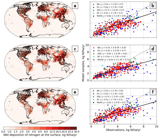
Figure 22 Geographical distribution of the wet-deposition flux of nitrogen for C-GC (a, b), S-GC (c, d), and C-CC (e, f). The annual mean value is shown as a map for each model, with circles used to indicate observational measurements (a, c, e). A parity plot of the results against the rainwater composition measurements is also provided for each model simulation (b, d, f).

5.4 Wet- and dry-deposition tendencies

Finally, we compare simulated and observed surface deposition. As deposition is the primary removal mechanism for atmospheric reactive nitrogen and sulfur species, the ability of a model to reproduce observed patterns of deposition provides an aggregate diagnostic for its representation of emissions, atmospheric chemistry, and the physical deposition processes.

Recent measurements have provided wet-deposition rates in numerous geographical locations for the years 2005 to 2007 (Vet et al., 2014). Dry-deposition fluxes are available from the same study but are limited to sulfur and nitrogen species. They are also limited to fewer geographical locations. Nonetheless, we compare results from all three model configurations to the results from Vet et al. (2014) below.

Figure 22 compares the model-evaluated wet-deposition rates of nitrogen at the surface for C-GC, C-CC, and S-GC. The total nitrogen flux is calculated by adding surface fluxes from each individual nitrogen compound undergoing wet deposition. Rainwater composition measurements are also displayed where available for comparison. We find correlation coefficients of 0.65, 0.66, and 0.67 for C-GC, C-CC, and S-GC, respectively, with these observations. On average, the results from C-GC (Fig. 22b) are closest to parity with a slope of 0.6, compared with respective values of 0.5 and 0.49 for C-CC (Fig. 22d) and S-GC (Fig. 22f). We do not find any clear trends by location between the three models.

Comparing the dry-deposition flux of nitrogen species at the surface from C-GC, C-CC, and S-GC to in situ measurements over North America (the only region present in this dataset) from 2005 to 2007 shows that all models have positive biases. Relative to an observational mean of 1.57 $\mathrm{kg}\mathrm{N}{\mathrm{ha}}^{-\mathrm{1}}{\mathrm{yr}}^{-\mathrm{1}}$, C-GC has the best performance with a mean bias of +0.94 $\mathrm{kg}\mathrm{N}{\mathrm{ha}}^{-\mathrm{1}}{\mathrm{yr}}^{-\mathrm{1}}$, compared with +1.76 and +2.32 $\mathrm{kg}\mathrm{N}{\mathrm{ha}}^{-\mathrm{1}}{\mathrm{yr}}^{-\mathrm{1}}$ from S-GC and C-CC, respectively. These biases from all three models can be explained by either larger concentrations of nitrogen compounds or enhanced dry-deposition velocities. However, we do not compensate for changes in nitrogen emissions between the time of the observations (2005–2007) and the simulated period, during which NO_x emissions are estimated to have increased (Emmons et al., 2020).

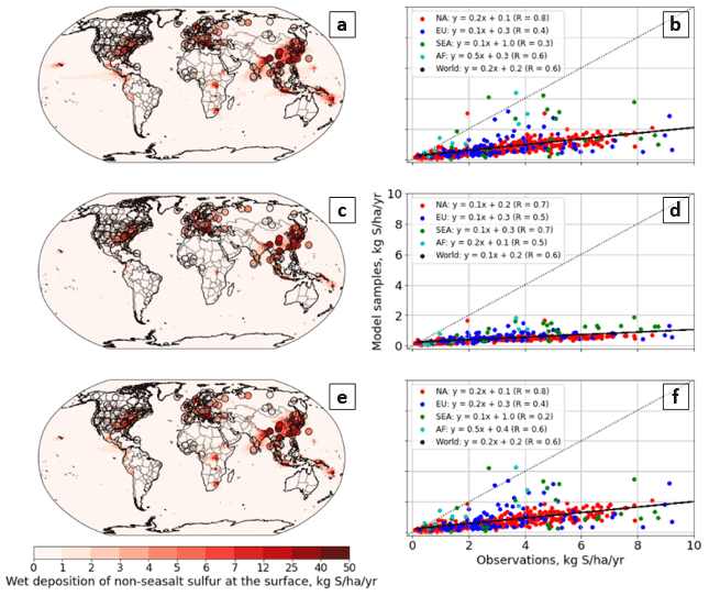
Figure 23 As in Fig. 22 but for non-sea-salt sulfur for C-GC (a, b), S-GC (c, d), and C-CC (e, f).

Figure 23 displays the evaluated wet-deposition rates of non-sea-salt sulfur from C-GC, C-CC, and S-GC alongside measurements of sulfur in rainwater for 2005. When comparing across model results, we find a global mean deposition rate of 0.58, 0.38, and 0.50 kg S ha yr⁻¹ in C-GC, S-GC, and C-CC, respectively (computed as the global surface average of Fig. 23a, c, and e). The results from C-GC and C-CC show a correlation coefficient greater than 0.95, whereas results from C-GC and S-GC show a correlation coefficient of 0.88.

Via comparison to observational data, we find a mean bias of −2.40 kg S ha yr⁻¹ (C-CC and C-GC) and −2.76 kg S ha yr⁻¹ (S-GC) between the simulation results and rainwater composition measurements. This bias is location-dependent, with simulated data for Asia showing a lower bias than North America or Europe. For instance, over North America, measurements indicate a mean sulfur wet-deposition flux of approximately 5 kg S ha yr⁻¹ (for the year 2005), whereas the results at the same stations are lower with the slope of the linear fit equal to 0.2, 0.1, and 0.2 for C-GC, S-GC, and C-CC, respectively. This can be explained by the reduction in the sulfur wet-deposition surface flux over the past decades. Previous literature has found that the deposition rate of sulfur over the eastern US has been decreasing at a rate of 1 kg S ha yr⁻¹ since 1990, with 60 % of the reduction being in wet-deposition rates and 40 % in dry-deposition rates (Zhang et al., 2018). Similar findings have been suggested for wet-deposition rates over Europe (Theobald et al., 2019). A similar, but more recent, decrease over Asia has also been observed (Aas et al., 2019).

It is difficult to say with confidence that the calculated bias is purely due to lack of recent data without new measurements to support this conclusion. However, our results do show that the simulation of sulfur deposition in C-GC more closely follows that in C-CC than that in S-GC. This could be due to either the simulated distribution of precipitation, the representation of aerosol, or the representation of scavenging processes, all of which differ between C-GC (or C-CC) and S-GC.

6 Discussion and conclusion

We present the first implementation of the GEOS-Chem chemistry mechanism as an option in the Community Earth System Model (CESM). In addition to allowing users of CESM to take advantage of advancements in atmospheric modeling implemented in the GEOS-Chem model, this also allows the community to better understand why models disagree and how progress might be made to improve model performance and accuracy.

Our results suggest that differences in the representation of tropospheric halogen chemistry – in particular the representation and magnitude of emissions of short-lived bromine and chlorine sources – may be responsible for differences in simulated ozone between these model configurations. However, in addition to the recognized differences in chemical mechanisms, subtle structural differences in atmospheric models may have a significant role. Our evaluation of tropospheric ozone concentrations suggests that one of the key drivers of the variation between CAM-chem and GEOS-Chem ozone fields differences may be differences in free tropospheric water vapor. Similarly, we show that sulfur deposition rates are approximately twice as great when running GEOS-Chem in a stand-alone model as opposed to running GEOS-Chem embedded in CESM, despite the use of identical emissions.

We also find that differences in the representation of wet scavenging are a significant contributor to variations in reactive nitrogen and halogen species distributions between GEOS-Chem and CAM-chem. The unification of convective transport and scavenging in GEOS-Chem helps to prevent the movement of soluble species to the upper troposphere through convective updrafts and, therefore, limits the effect of near-surface halogen emissions from sea salt on ozone at higher altitudes.

Our implementation of GEOS-Chem in CESM is now publicly available for use. We envision that this model can become a powerful tool for research, forecast, and regulatory applications of global atmospheric chemistry, air quality, and climate research. Furthermore, this is also an important step towards the Multi-scale Infrastructure for Chemistry and Aerosols (MUSICA) and, therefrom, a truly modular Earth system model (Pfister et al., 2020). By enabling us to fairly compare models down to individual processes, we can begin to understand precisely why different models perform better or worse in reproducing different measurements and accelerate our efforts to improve atmospheric modeling fidelity as a whole.

Finally, this work will foster collaboration between the GEOS-Chem and CESM CAM-chem communities. GEOS-Chem is presently used and developed worldwide for research by over 100 university groups and government agencies, and CAM-chem similarly has numerous users and developers. The availability of GEOS-Chem as an option in CESM will stimulate broader interest in the use of CESM from the GEOS-Chem community as well as in the use of GEOS-Chem from the CESM community. Indeed, we expect that online simulation of atmospheric chemistry will become increasingly attractive to GEOS-Chem users as the resolution of dynamical models increase and that CESM will provide the principal vehicle for this because of its public availability and support. By enabling improvements developed for GEOS-Chem to percolate into CESM without the need for re-implementation, this work will accelerate progress in atmospheric chemistry and Earth system modeling.