the Creative Commons Attribution 4.0 License.
the Creative Commons Attribution 4.0 License.
 | 31 Jan 2022
The importance of turbulent ocean–sea ice nutrient exchanges for simulation of ice algal biomass and production with CICE6.1 and Icepack 1.2
Philipp Assmy
Karley Campbell
Arild Sundfjord
Different sea ice models apply unique approaches in the computation of nutrient diffusion between the ocean and the ice bottom, which are generally decoupled from the calculation of turbulent heat flux. A simple molecular diffusion formulation is often used. We argue that nutrient transfer from the ocean to sea ice should be as consistent as possible with heat transfer, since all of these fluxes respond to varying forcing in a similar fashion. We hypothesize that biogeochemical models that do not consider such turbulent nutrient exchanges between the ocean and the sea ice, despite considering brine drainage and bulk exchanges through ice freezing and melting, may underestimate bottom-ice algal production. The Los Alamos Sea Ice Model (CICE + Icepack) was used to test this hypothesis by comparing simulations without and with diffusion of nutrients across the sea ice bottom that are dependent on velocity shear, implemented in a way that is consistent with turbulent heat exchanges. Simulation results support the hypothesis, showing a significant enhancement of ice algal production and biomass when nutrient limitation was relieved by bottom-ice turbulent exchange. Our results emphasize the potentially critical role of turbulent exchanges to sea ice algal blooms and thus the importance of properly representing them in biogeochemical models. The relevance of this becomes even more apparent considering ongoing trends in the Arctic Ocean, with a predictable shift from light-limited to nutrient-limited growth of ice algae earlier in the spring, as the sea ice becomes more fractured and thinner with a larger fraction of young ice with thin snow cover.
- Article
(10128 KB) - Full-text XML
-
Supplement
(832 KB) - BibTeX
- EndNote


Momentum, heat, and mass fluxes between the ocean and sea ice are of utmost importance to predict sea ice motion, thermodynamics, and biogeochemistry. However, when we look at models released over the last few decades, we find not only inter-model differences in the physical concepts used to describe the processes responsible for some of the above fluxes but also intra-model differences in the approaches used in calculating, for example, heat and mass fluxes. In this work we will focus on the differences related to the vertical diffusion of tracers between the water column and the bottom ice and attempt to explore their consequences on nutrient limitation for sea ice algal growth.
We may divide the ocean–ice exchange processes into those related to (i) entrapment during freezing; (ii) flushing and release during melting; (iii) brine gravity drainage, driven by density instability, parameterized as either a diffusive or a convective process; (iv) molecular diffusion; and (v) turbulent diffusion at the interface between the ocean and the ice induced by velocity shear – the latter process being the focus of this study (e.g., Arrigo et al., 1993, and references therein; Jin et al., 2006; McPhee, 2008; Notz and Worster, 2009; Turner et al., 2013; Tedesco and Vichi, 2010, 2019; Jeffery et al., 2011; Vancoppenolle et al., 2013).
These processes are considered in several sea ice models. Arrigo et al. (1993) distinguished nutrient exchanges resulting from gravity drainage in brine channels from brine convection in the skeletal layer using the ice growth rate. These brine fluxes were used to calculate nutrient exchanges as a diffusive process. Lavoie et al. (2005) also calculated nutrient exchanges as a diffusive process. Jin et al. (2006, 2008) computed nutrient fluxes across the bottom layer as an advection process dependent on ice growth rate based on the work of Wakatsuchi and Ono (1983). Molecular diffusion was also considered. More recently, other authors have integrated formulations of “enhanced diffusion” (Vancoppenolle et al., 2010; Jeffery et al., 2011) or convection (Turner et al., 2013), based on hydrostatic instability of brine density profiles, to compute brine gravity drainage and tracer exchange within the ice and between the ice and the seawater. Comparisons between salt dynamics in growing sea ice with salinity measurements showed that convective Rayleigh number-based parameterizations (e.g., Wells et al., 2011), such as the one by Turner et al. (2013), outperform diffusive and simple convective formulations (Thomas et al., 2020).
Interestingly, heat exchange is often calculated differently from salinity in models. In the case of the former, typically a transfer mechanism (turbulent or not) at the interface between the ocean and the sea ice is not dependent on any type of brine exchange. In the latter, such a mechanism is not considered (e.g., Vancoppenolle et al., 2007; Turner et al., 2013). Presumably, such differences result from the relative importance of various physical processes for different tracers. Heat transfer between the ice and the water is a fundamental mechanism in explaining sea ice thermodynamics, irrespective of brine exchanges. On the other hand, ice desalination depends mostly on brine gravity drainage and flushing during melting (Notz and Worster, 2009).
Vertical convective mixing of nutrients under the sea ice may result from brine rejection and/or drainage from the sea ice (Lake and Lewis, 1970; Niedrauer and Martin, 1979; Reeburgh, 1984) and from turbulence due to shear instabilities generated by drag at the interface between the ocean and the sea ice (Gosselin et al., 1985; Cota et al., 1987; Carmack, 1986), internal waves, and topographical features (Ingram et al., 1989; Dalman et al., 2019). Gosselin et al. (1985) and Cota et al. (1987) stressed the significance of tidally induced mixing in supplying nutrients to sympagic algae. Biological demand for silicic acid (hereafter abbreviated as silicate) and nitrate is limited by the physical supply (Cota and Horne, 1989; Cota and Sullivan, 1990).
The analysis of several models published over the last few decades and their approaches to calculate tracer diffusion across the ice–ocean interface shows that some models do not consider this process or limit it to molecular diffusion. Other models consider turbulent exchanges parameterized as a function of the Rayleigh number, calculated from brine vertical density gradients. Only two of the sampled models (Lavoie et al., 2005; Mortenson et al., 2017) use parameterizations based on friction velocity. The former uses eddy diffusion to simulate the vertical supply of nutrients to the molecular sublayer, where nutrient fluxes and their supply to the bottom ice are limited by molecular diffusion. The latter uses a coupled ocean–sea ice model, but molecular diffusion is ultimately the controlling process. Both authors use the same approach to compute the thickness of the molecular sublayer based on friction velocity.
In the absence of ice growth and when brine gravity drainage is limited, diffusive nutrient exchanges between the ocean and the ice have the capacity to limit primary production. This limitation will be alleviated in the presence of a turbulent exchange mechanism. We argue that nutrient transfer at the interface between the ocean and the sea ice should be as consistent as possible with heat transfer since all these fluxes are closely linked. We hypothesize that models that do not consider the role of current velocity shear on turbulent nutrient exchanges between the ocean and the sea ice may underestimate bottom-ice algal production.
To test the above hypothesis, we use a 1D vertically resolved model implemented with the Los Alamos Sea Ice Model (CICE + Icepack) and contrast results using the default diffusion parameterization and a “turbulent” parameterization analogous to that of heat and salt transfer at the interface between the ocean and sea ice based on McPhee (2008). This implementation of the turbulent parameterization is specific for the software used, and it may be different in other models.
2.1 Concepts
Turbulent exchanges may be parameterized through the flux of a quantity at the interface between the ocean and the sea ice, calculated as the product of a scale velocity and the change in the quantity from the boundary to some reference level (McPhee, 2008):
where represents the averaged co-variance of the turbulent fluctuations of interface vertical velocity (m s−1) and salinity, αs is an interface salt–nutrient exchange coefficient (dimensionless), u∗ is the friction velocity (m s−1), and So and Sw are interface and far-field salinities, respectively.
We calculate nutrient exchanges using a similar approach:
This is an extension of the concept used for heat and salt by McPhee (2008; see p. 112, Fig. 6.3). The minus sign used in Eq. (2) is for compatibility with the CICE + Icepack convention that upward fluxes be negative (e.g., Hunke et al., 2015). αs varies from during the melting season to 0.006 during winter (McPhee et al., 2008).
Before explaining how Eq. (2) was implemented in the CICE + Icepack we describe the model vertical biogeochemical grid (biogrid), the tracer equation and the bottom boundary conditions. The biogrid is the non-dimensional grid used for discretizing the vertical transport equations of biogeochemical tracers, defined between the brine height (h), which takes the value 0, and the ice–ocean interface, which takes the value 1 (Jeffery et al., 2016). The Icepack tracer equation (without biogeochemical reaction terms for the sake of simplicity) may be written as follows (for more details, see Jeffery et al., 2011, 2016):
where is the relative depth of the vertical domain of the biogrid, zt and zb are vertical positions of the ice top and bottom (m), respectively, ϕ is sea ice porosity, wf is the Darcy velocity due to the sea ice flushing of tracers (m s−1), Dm is the molecular diffusion coefficient, and DMLD is the mixed length diffusion coefficient (m2 s−1). DMLD is detailed in Jeffery et al. (2011), and it is 0 when the brine vertical density gradient is stable, otherwise (when density increases towards the ice top) it is calculated as follows:
where g is the acceleration of gravity (9.8 m s−2), k is sea ice permeability, μ is dynamic viscosity (2.2 kg m−1 s−1), ρe is the equilibrium brine density, and l is a length scale (7 m). The values shown here are the default ones in CICE + Icepack.
The bottom boundary condition of Eq. (3) is based on values of N at the sea ice bottom interface (N0 at x=1) and in the ocean (Nw) (Jeffery et al., 2011). Therefore, the last term of Eq. (3) at the bottom boundary may be written as follows:
In CICE + Icepack, diffusion timescales are calculated separately for later usage in Eq. (3) as follows:
and
A similar timescale for the turbulent process described by Eq. (2) may be calculated from the following equation:
Therefore, in the Los Alamos Sea Ice Model the implementation of turbulent diffusion nutrient exchanges at the ice–ocean interface is quite straightforward. In other models, other approaches may be required.
The usage of h in these timescales merely implies the way they are normalized in the code before the actual diffusive fluxes are calculated considering the distance between the points (h∂x; see Eq. 3) where variables are calculated along the layers of the biogrid. The product h⋅x corresponds to the actual distance of a given point from the top of the biogrid.
In the simulations using turbulent diffusion, we perform the same calculations, except that the molecular diffusion term is replaced with a turbulent diffusion term at the interface between the last model layer and the ocean. This exchange process takes place “outside” the sea ice where φ=1, directly affecting only the tracer concentration at the ice–ocean interface.
From Eqs. (6)–(8) it turns out that the product αsu∗ by distance (z) has the same dimensions as Dm or DMLD, corresponding to a turbulent diffusion coefficient. Assuming z≈0.01 m, turbulent diffusion induced by velocity shear becomes comparable with molecular diffusion only for m s−1 considering the lower end of the αs range (; see above) or m s−1 considering the upper end of the αs range (0.006). If we instead assume z≈0.00054 m (the average thickness of the molecular sublayer reported in Lavoie et al., 2005), the calculated u∗ values increase by 1 to 2 orders of magnitude (depending on αs) but are still low (0.0004–0.03 m s−1). In fact, such low friction velocities would require low “stream” velocities, i.e., relative ice–ocean velocities. For an account of the relationship between stream and friction velocities under the sea ice, see Supplement 3 of Olsen et al. (2019) and references therein. These authors show that stream velocities of only a few centimeters per second lead to friction velocities that are an order of magnitude lower but are still on the order of 0.001 m s−1, i.e., smaller only than the highest u∗ values estimated above. Considering current velocities relative to the sea ice observed during the N-ICE2015 cruise (Granskog et al., 2018; Fig. 2d of Duarte et al., 2017), with most values between 0.05 and >0.2 m s−1, it is rather likely that friction velocities under the ice are frequently above the thresholds calculated above and that turbulent diffusion will dominate over molecular diffusion. Dalman et al. (2019) provided experimental evidence for such turbulent nutrient fluxes to the ice bottom, leading to increased chlorophyll concentrations at the bottom ice in a strait with strong tidal currents. The mechanism treated here as turbulent diffusion seems analogous to “forced convection” in the lowermost parts of the brine network, which is driven by pressure differences caused by the shear under the sea ice (Vancoppenolle et al., 2013).
2.2 Implementation
We used the Los Alamos Sea Ice Model, which is managed by the CICE Consortium with an active forum (https://bb.cgd.ucar.edu/cesm/forums/cice-consortium.146/, last access: 26 January 2022), and a Git repository (https://github.com/CICE-Consortium, last access: 26 January 2022). It includes two independent packages: CICE and Icepack. The former computes ice dynamic processes, and the latter computes ice column physics and biogeochemistry. Their development is handled independently with respect to the GitHub repositories (https://github.com/CICE-Consortium). All of the changes described below were implemented in two forks to the above repository, one for Icepack and another for CICE, and they may be found in Duarte (2021a) and Duarte (2021b), respectively.
Our simulations may be run using only Icepack, since they are focused on ice column physics and biogeochemistry, without the need to consider ice dynamic processes. However, we used both CICE + Icepack together to allow for use of a netCDF-based input/output not included in Icepack. Therefore, we defined a 1D vertically resolved model with 1 snow layer and 15 ice layers and 5×5 horizontal cells. This is the minimum number of cells allowable in CICE due to the need to include halo cells (only the central “column” is simulated). Therefore, ice column physics and biogeochemistry were calculated by Icepack, but CICE was the model driver. The input file (ice_in) used in this study was included in our CICE fork and it lists all parameters used in the model and described in Hunke et al. (2015), Jeffery et al. (2016), and Duarte et al. (2017) and in Tables S1 and S2. Any changes in “default” parameters or any other model settings will be specified.
We made several modifications in CICE to allow using forcing time series collected during the Norwegian young sea ice (N-ICE2015) expedition (Granskog et al., 2018) and described in Duarte et al. (2017) (see Fig. 2 of the cited authors). These modifications were meant to allow reading of forcing data at higher frequencies than possible with the standard input subroutines in the CICE file ice_forcing.F90.
When the dynamical component of CICE is not used, u∗ is set to a minimum value instead of being calculated as a function of ice–ocean shear stress (Hunke et al., 2015). Duarte et al. (2017) implemented shear calculations from surface current velocities (one of the models forcing functions) irrespective of the use of the CICE dynamics code. These modifications were also incorporated in the current model configuration so that shear can be used to calculate friction velocity and thereafter influence heat and tracer–nutrient exchanges, following Eqs. (2) and (8) and parameters described in McPhee et al. (2008). When the parameter kdyn is set to 0 in ice_in, ice dynamics are not computed, but shear is calculated in the modified subroutine icepack_step_therm1, file icepack_therm_vertical.F90. If kdyn is not 0, these calculations are ignored since shear is already calculated in the dynamical part of the CICE code.
A Boolean parameter (Bottom_turb_mix) was added to the input file, which is set to “false” or “true” when the standard molecular diffusion approach or the new turbulence-based diffusion approach is used, respectively. Another Boolean parameter (Limiting_factors_file) was added to the ice_in file. When set to true, limiting factor values for light, temperature, nitrogen, and silicate are written to a text file every model time step. These are calculated by Icepack biogeochemistry, according to Jeffery et al. (2016), but there is no writing output option in the standard code.
2.3 Model simulations
Simulations were run for a refrozen lead (RL) without snow cover and for second-year sea ice (SYI) with ∼40 cm snow cover monitored in April–June during the N-ICE2015 expedition (Granskog et al., 2018, and Fig. 1 of Duarte et al., 2017). Details of model forcing with atmospheric and oceanographic data collected during the N-ICE2015 expedition, including citations and links to the publicly available datasets, are given in Fig. 2 and Sect. 3 of Duarte et al. (2017) and in the Supplement. These datasets include wind speed, air temperature, precipitation, and specific humidity in Hudson et al. (2015); incident surface short and longwave radiation in Hudson et al. (2016); ice temperature and salinity in Gerland et al. (2017); sea surface current velocity, temperature, salinity, and heat fluxes from a turbulence instrument cluster (TIC) in Peterson et al. (2016); sea surface nutrient concentrations in Assmy et al. (2016); and sea ice biogeochemistry in Assmy et al. (2017). Ocean forcing is based on measurements within the surface 2 m that provide the boundary condition for the sea ice model. Model forcing files may be found in Duarte (2021c).
RL simulations started with zero ice, whereas SYI simulations started with initial conditions described in the Supplement (Table S3).
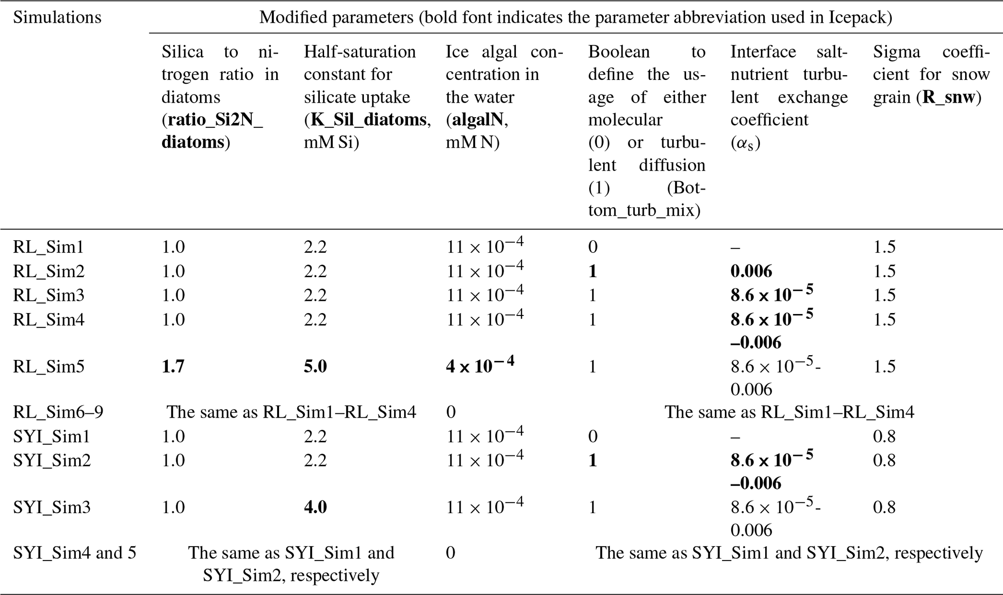
Table 1Model simulations. Refrozen lead (RL) simulation RL_Sim1 corresponds to RL_Sim5 described in Duarte et al. (2017), which was the simulation leading to a best fit to the observations in that study. The remaining RL simulations 2–5 differ from RL_Sim1 in that they use turbulent diffusion for nutrients at the interface between the ocean and the sea ice. Moreover, RL_Sim5 differs in the concentration of ice algae in the water column that colonize the sea ice bottom (algalN) and in silicate-limitation-related parameters. These changes were done iteratively to fit the model to the observations. In RL_Sim2 and RL_Sim3 the maximum (αs=0.006) and the minimum () values recommended by McPhee et al. (2008), respectively, are used throughout the simulations to provide extreme case scenarios for comparison with RL_Sim1. In RL_Sim4, when ice is not growing and 0.006 otherwise, as recommended by McPhee et al. (2008), to account for double diffusive processes during ice melting that slow down mass exchanges. The remaining RL simulations (R__Sim6–9) are like the previous ones (RL_Sim1–4), except for algalN being set to 0 mmol N m−3 and all simulations being restarted with the same values for all variables. Therefore, simulations 6–9 may differ only from 13 May 2015, which is when they were restarted. Second-year ice simulation SYI_Sim_1 is based on Duarte et al. (2017) SYI_Sim4 but without algal motion. SYI_Sim2 and SYI_Sim3 use turbulent diffusion at the interface between the ocean and the sea ice. The former uses a decreased half-saturation constant for silicate uptake, just like SYI_Sim1, whereas the latter uses the standard CICE value. The remaining SYI simulations (SYI__Sim4 and 5) are like SYI_Sim1and 2, except that algalN was set to 0. Simulations SYI_Sim1 and SYI_Sim2 were repeated but with different initial snow thicknesses of 30, 20, and 15 cm to further investigate the interplay between light and silicate limitation (see Sect. 2.3). Modified parameter values from one simulation to the next are marked in bold (separately for RL and SYI simulations). Modified parameters are based on literature ranges (e.g., Brzezinski, 1985; Hegseth, 1992, for ratio_Si2N_diatoms; Nelson and Treguer, 1992, for K_Sil_diatoms; and Urrego-Blanco et al., 2016, for R_snw) or on previous model calibration work (Duarte et al., 2017). Parameters values were modified in the model input file ice_in, except for algalN and αs, which are hard-coded.
We ran simulations with the standard formulations for biogeochemical processes described in Jeffery et al. (2016) and settings described in Duarte et al. (2017) using mushy thermodynamics and vertically resolved biogeochemistry and including freezing, flushing, brine mixing length, and molecular diffusion within the ice and at the interface between the ocean and the sea ice as nutrient exchange mechanisms (Jeffery et al., 2011, 2016). We contrasted the above simulations against others that replaced brine molecular and mixed-length diffusion of nutrients at the interface between the ocean and the sea ice with diffusion driven by current velocity shear (Table 1) calculated similar to heat exchanges and following the parameterization described in McPhee et al. (2008) and detailed above (Eqs. 2–7). This contrast provides insight into the effects of velocity shear on nutrient diffusion, ice algal production (mg C m−2 d−1), chlorophyll standing stocks (mg Chl a m−2), and vertical distribution of chlorophyll concentration (mg Chl a m−3) (note that CICE model output for algal biomass in mmol N m−3 was converted to mg Chla m−3 as in Duarte et al., 2017, using 2.1 mg Chl a mmol N−1 and following Smith et al., 1993). However, due to the concurrent effects of algal biomass exchange between the ocean and ice, such a contrast is not enough to explicitly test our hypothesis and conclude about the effects of turbulence-driven nutrient supply on ice algal nutrient limitation. Therefore, simulations were also run contrasting the same model setups, as described above but restarting from similar algal standing stocks and vertical distributions within the ice and switching off algal inputs from the water to the ice. This was done by nullifying the variable algalN, defining the ocean surface background ice algal concentration, in file icepack_zbgc.F90, subroutine icepack_init_ocean_bio, and the restart files. In the case of the RL simulations that started with zero ice, first a simulation was run until the 12 May, and then the obtained ice conditions were used to restart new simulations without algal inputs from the ocean (algalN = 0 mmol N m−3). Therefore, when the simulations restarted there was already an ice algal standing stock necessary for the modeling experiments developed herein. The SYI simulations were by default “restart simulations” beginning with observed ice physical and biogeochemical variables. Therefore, there was already an algal standing stock in the ice from the onset (Sect. S1 and Table S3).
McPhee et al. (2008) estimated different values for αs depending on whether the sea ice is growing (highest value) or melting (lowest value) (Table 1). When running simulations for the RL, in some cases we used only the minimum or the maximum values for αs to allow for a more extreme contrast between molecular and turbulent diffusion parameterizations. This was done since the former value will tend to minimize differences, whereas the latter will tend to emphasize them. We also completed simulations for the RL and for SYI changing between the maximum and the minimum values of αs when ice was growing or melting, respectively, and following McPhee et al. (2008) (see Table 1 for details). This parameterization with variable αs is likely the most realistic one, accounting for double diffusion during ice melting (McPhee et al., 2008).
Apart from contrasting the way bottom-ice exchanges of nutrients were calculated, some simulations contrasted different parameters related to silicate limitation (Table 1). This approach follows Duarte et al. (2017), where simulations were tuned by changing the Si:N ratio and the half-saturation constant for silicate uptake because silicate limitation was leading to an underestimation of algal growth. From this exercise we were able to assess if such tuning was still necessary after implementing turbulent diffusion at the interface between the ocean and the sea ice, driven by velocity shear. Moreover, we repeated simulations with varying snow heights to further investigate the interplay between light and nutrient limitation under contrasting nutrient diffusion parameterizations (Table 1).
The results of the simulations listed in Table 1 and presented below may be found in Duarte (2021d).

Figure 1Daily averaged results for the refrozen lead (RL): (a) observed and modeled Chl a concentration values averaged for the ice bottom 10 cm, and (b) observed and modeled Chl a standing stock (continuous lines) and modeled net primary production (NPP) (dashed lines) for the whole ice column (refer to Table 1 for details about model simulations). Observations are the same as those presented in Duarte et al. (2017).
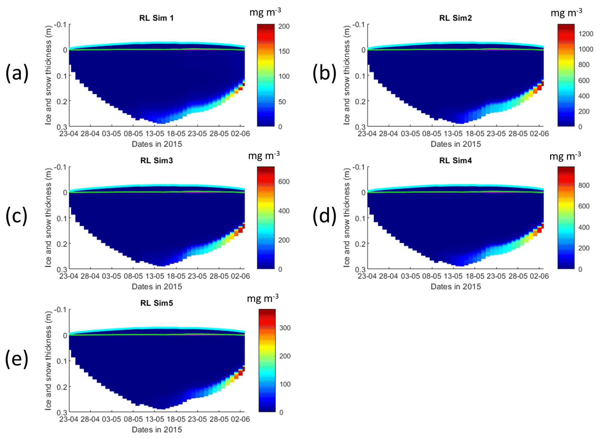
Figure 2Daily averaged results for the refrozen lead (RL) simulations 1–5. Simulated evolution of ice algae Chl a is given as a function of time and depth in the ice (note the color scale differences between the various panels). Ice thickness is given by the distance between the upper and the lower limits of the maps. The upper regions of the graphs above the green line with zero values are above the CICE biogrid and have no brine network. The magenta line, which is partly covered by the green line, represents sea level. Refer to Table 1 for details about model simulations.
3.1 Refrozen lead simulations
All simulations with turbulent diffusion (RL_Sim2–RL_Sim5, Table 1) predict higher bottom chlorophyll a (Chl a) concentration than with the standard molecular diffusion formulation (RL_Sim1) (Fig. 1a). Simulations RL_Sim2–4 grossly overestimate observations. Simulation RL_Sim3, using the lowest value for αs, is closer both to observations and to RL_Sim1, as well as RL_Sim5, with the latter having the same αs values of RL_Sim4 but a half-saturation constant for silicate limitation increased from its tuned value in Duarte et al. (2017) of 2.2 to 5.0 µM and algalN reduced (Table 1) to bring model results closer to observations. Patterns between simulations for the whole ice column and considering both standing stocks and net primary production are similar to those observed for the bottom ice (Fig. 1b). Algal biomass is concentrated at the bottom layers (Fig. 2). Concentrations in the layers located between the bottom and the top of the biogrid, defined by the vertical extent (brine height) of the brine network (green lines in the map plots) (Jeffery et al., 2011), are <10 mg Chl a m−3. Ice thickness, temperature, and salinity profiles are extremely similar among these simulations (Figs. S1 and S2).
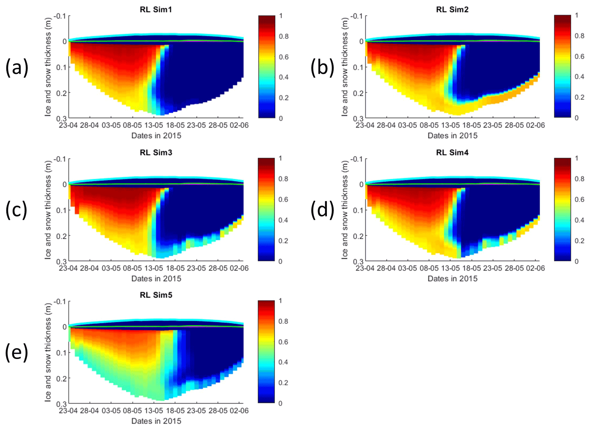
Figure 3Daily averaged results for the refrozen lead (RL) simulations 1–5. Simulated evolution of silicate limitation (1 being no limitation, and 0 being maximal limitation) is given as a function of time and depth in the ice. Ice thickness is given by the distance between the upper and the lower limits of the maps. The upper regions of the graphs above the green line with zero values are above the CICE biogrid and have no brine network. The magenta line, which is partly covered by the green line, represents sea level. Refer to Table 1 for details about model simulations.
Results for the silicate- and nitrogen-limiting factors are based on brine concentrations. Limiting factors exhibiting lower values (more limitation) in RL simulations are silicate, followed by light (Figs. 3, S3–S5). Limiting values for silicate range between 0 (maximum limitation) and 1 (no limitation), with stronger limitation after 13 May in all simulations (Fig. 3). The most severe silicate limitation is for RL_Sim1, where values drop to near zero around middle May. Despite the high average bottom Chl a concentration predicted in all simulations, the bottom layer is where silicate limitation is less severe after 13 May. This is more evident in simulations with turbulent bottom diffusion, where light limitation at the bottom ice becomes more severe than silicate limitation around the end of May (Fig. S6).
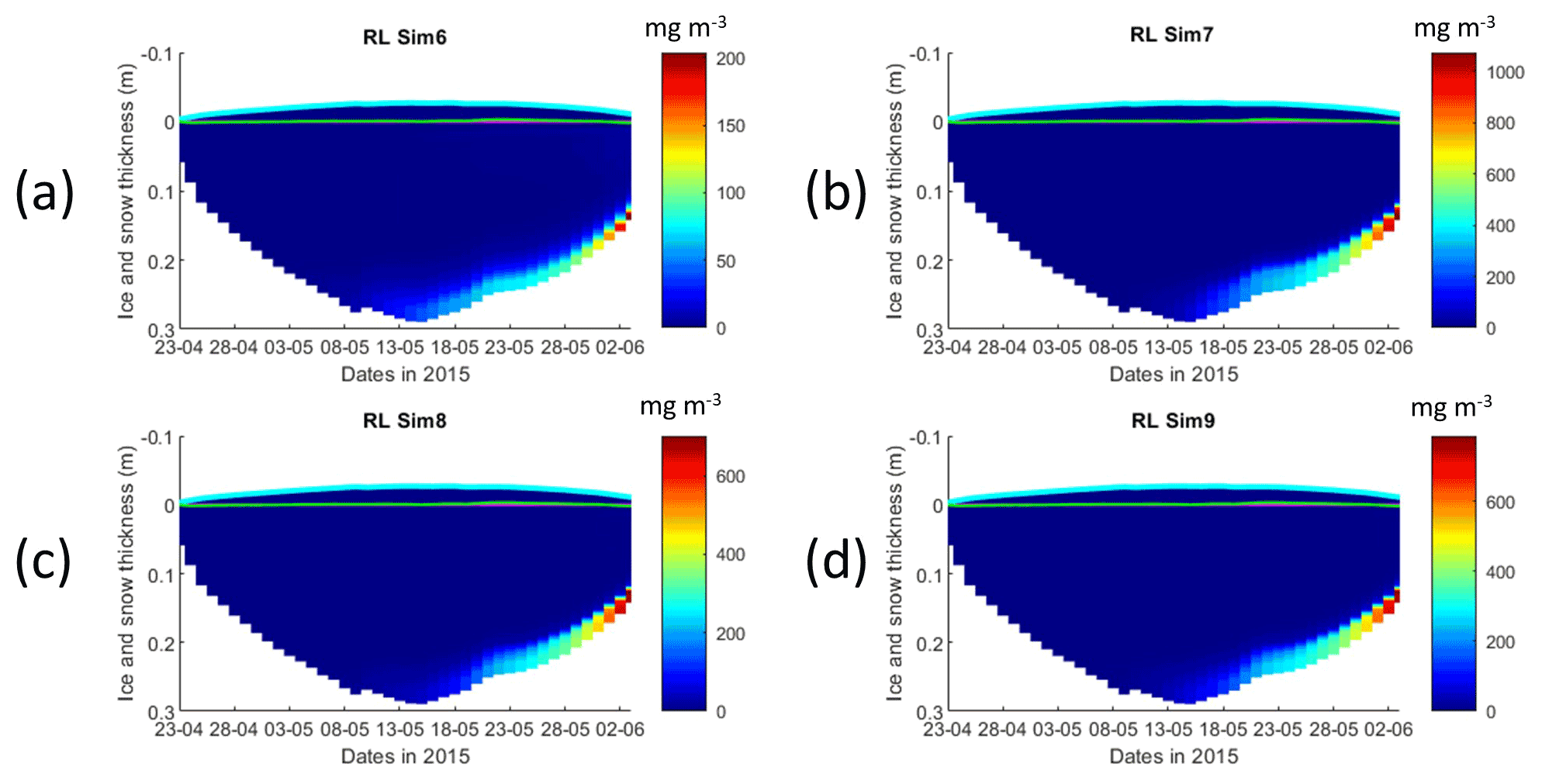
Figure 4Daily averaged results for the refrozen lead (RL) simulations 6–9. Simulated evolution of ice algae Chl a is given as a function of time and depth in the ice (note the color scale differences between the various panels). Ice thickness is given by the distance between the upper and the lower limits of the maps. The upper regions of the graphs above the green line with zero values are above the CICE biogrid and have no brine network. The magenta line, which is partly covered by the green line, represents sea level. Refer to Table 1 for details about model simulations.
Results obtained with RL_Sim6–9 without algal exchanges between the ocean and the ice (see Table 1) show similar patterns of those observed with RL_Sim1–5, respectively (Fig. 4 versus Fig. 2, Fig. S9 versus Fig. 3, Figs. S7 and S8 versus Figs. S1 and S2, and Figs. S10–S12 versus Figs. S3–S5).
Interface diffusivity (one of CICE diagnostic variables, corresponding to the diffusion coefficient between adjacent biogeochemical layers and between the bottom layers and the ocean) for simulations with turbulent exchanges (αsu∗H) are up to 2 orders of magnitude higher at the bottom (diffusivity between the bottom layer and the ocean) than for the RL_Sim1 simulation with only molecular diffusion (Dm) + the mixed-length diffusion coefficient (DMLD) (see Sect. 2.1 and Fig. 5).
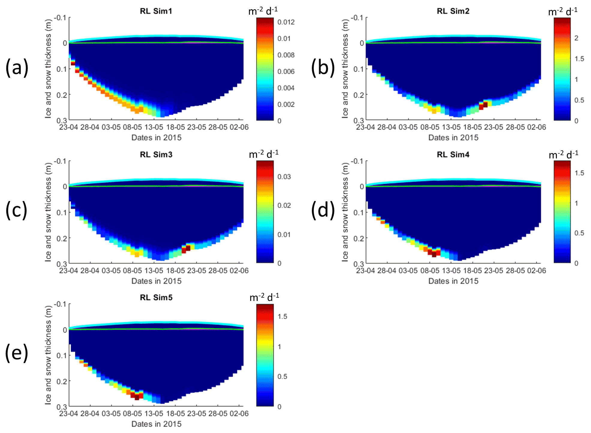
Figure 5Daily averaged results for the refrozen lead (RL) simulations 1–5. Simulated evolution of interface diffusivity is given as a function of time and depth in the ice (note the color scale differences between the various panels). Ice thickness is given by the distance between the upper and the lower limits of the maps. The upper regions of the graphs above the green line with zero values are above the CICE biogrid and have no brine network. The magenta line represents sea level. Refer to Table 1 for details about model simulations.
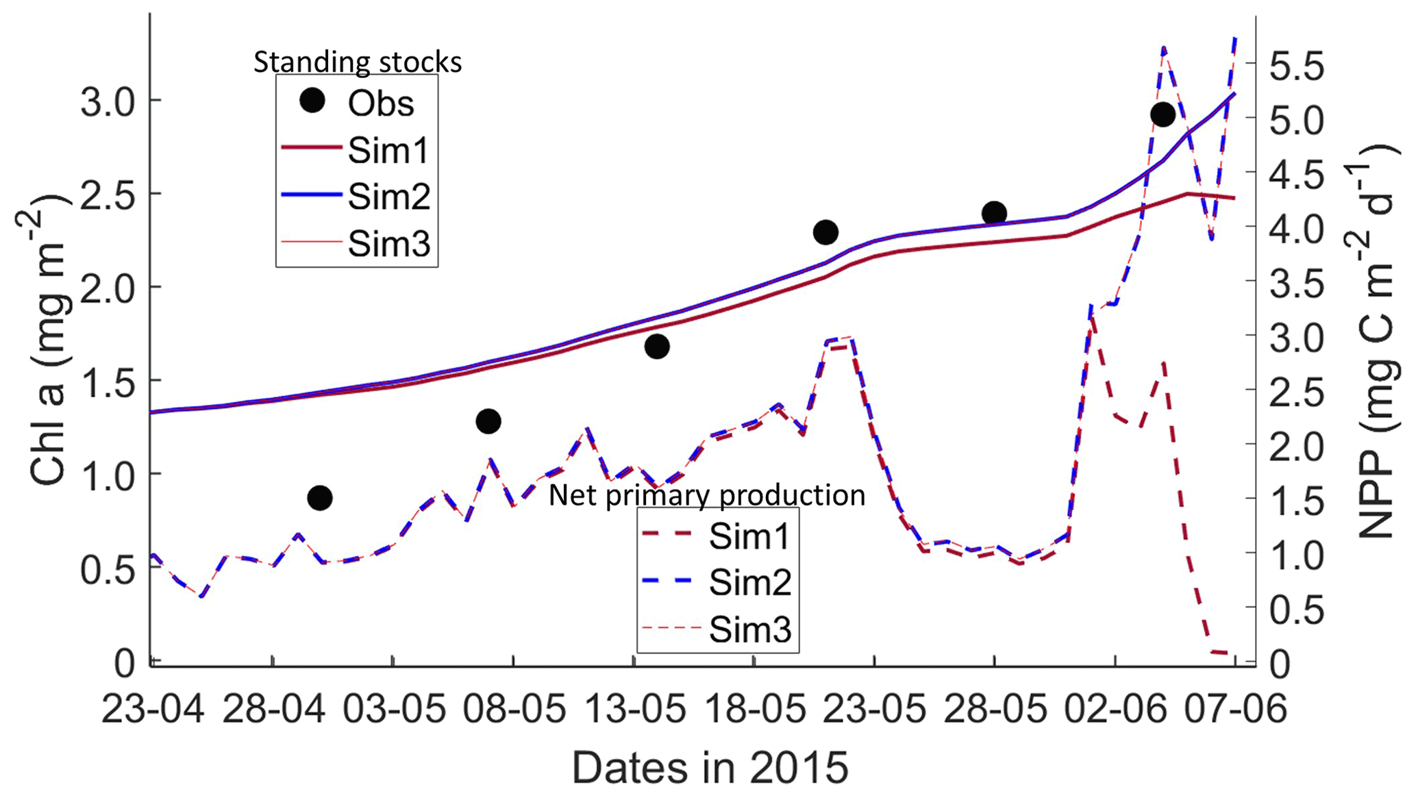
Figure 6Daily averaged results for second-year ice (SYI) simulations 1–3. Observed (same data presented in Duarte et al., 2017) and modeled Chl a standing stock (continuous lines) and modeled net primary production (NPP) (dashed lines) for the whole ice column are shown (refer to Table 1 for details about model simulations).
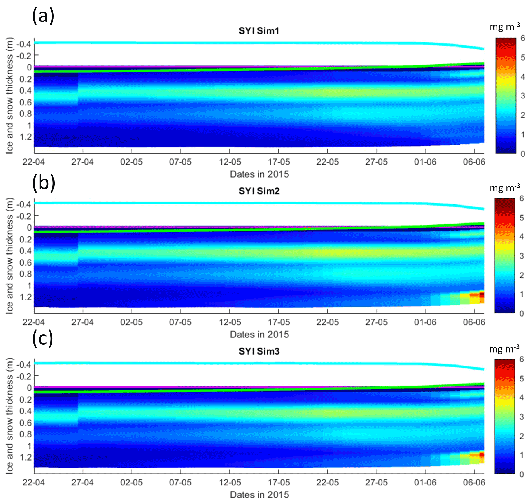
Figure 7Daily averaged results for second-year ice (SYI) simulations 1–3. Simulated evolution of ice algae Chl a is given as a function of time and depth in the ice. The upper regions of the graphs above the green line with zero values are above the CICE biogrid and have no brine network. The magenta line represents sea level, and the cyan line represents the top of the snow layer. Refer to Table 1 for details about model simulations.
3.2 Second-year ice simulations
Simulations with turbulent diffusion (SYI_Sim2 and 3) predict only slightly higher standing stocks and net primary production than with the standard molecular diffusion formulation (SYI_Sim1) (Fig. 6). The visual fit to the standing stock observations is comparable between the various simulations. Changing the half-saturation constant for silicate limitation from 2.2 to 4.0 µM has no impact on model results. This is confirmed by analyzing the evolution of Chl a concentration as a function of time and depth in the ice (Fig. 7), with only minor differences being apparent towards the end of the simulation, when Chl a increases at the bottom layers in the simulations with turbulent diffusion (SYI_Sim 2 and 3). Ice thickness, temperature, and salinity profiles are extremely similar among these simulations (Fig. S13).
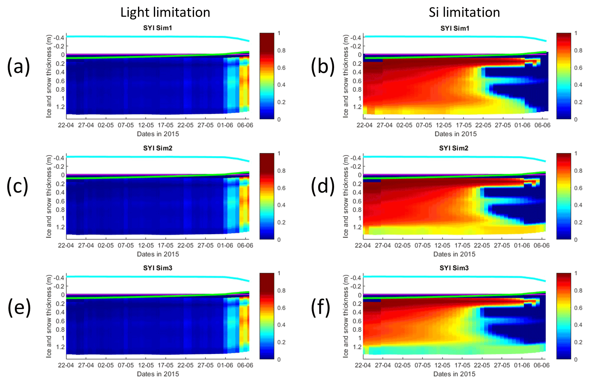
Figure 8Daily averaged results for second-year ice (SYI) simulations 1–3. Simulated evolution of light (a, c, e) and silicate (b, d, f) limitation (one means no limitation and zero is maximal limitation) are given as a function of time and depth in the ice. The upper regions of the graphs above the green line with zero values are above the CICE biogrid and have no brine network. The magenta line represents sea level, and the cyan line represents the top of the snow layer. Refer to Table 1 for details about model simulations.
The dominant limiting factor in these simulations is light, followed by silicate (compare Fig. 8a, c, and e with 8b, d, and f and with Fig. S14). Light limitation is less severe after the onset of snow and ice melting at the beginning of June. Silicate limitation is very strong above the bottom ice. Nitrogen limitation is highest at a depth range between ∼0.4–0.7 m below the ice top, with a large overlap with the depth range where a Chl a maximum is observed (Fig. 7). Maximal Chl a concentration predicted for the RL_Sim1 and RL_Sim5 simulations – those closer to observations – are 2 orders of magnitude higher than those predicted for SYI (Fig. 2a and e versus Fig. 7). However, standing stocks predicted for RL_Sim1 and RL_Sim5 simulations are smaller than for SYI simulations, as confirmed by the observations (Figs. 1b and 6). Opposite to what was described for the RL simulations, silicate limitation becomes more severe than light limitation at the bottom layer only in SYI_Sim_1 at the beginning of June close to the end of the simulation (Fig. S15).
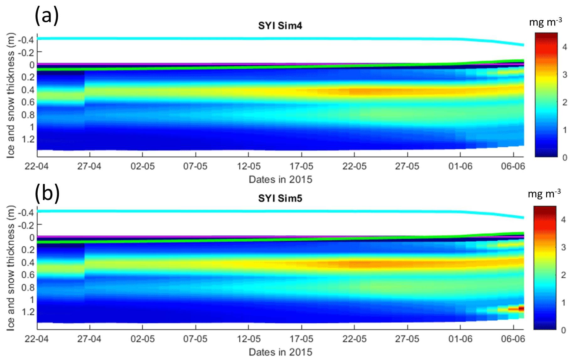
Figure 9Daily averaged results for second-year ice (SYI) simulations 4 and 5. Simulated evolution of ice algae Chl a as a function of time and depth in the ice. The upper regions of the graphs above the green line with zero values are above the CICE biogrid and have no brine network. The magenta line represents sea level, and the cyan line represents the top of the snow layer. Refer to Table 1 for details about model simulations.
Results obtained without algal exchanges between the ocean and the ice (SYI_Sim4 and 5; see Table 1), show the same patterns as those observed with SYI_Sim1 and 2, respectively (Fig. 9 versus Fig. 7, Fig. S17 versus Fig. 8, Fig. S18 versus Fig. S14a–d, and Fig. S16 versus Fig. S13a–d).
Interface diffusivity (one of CICE diagnostic variables; see Sect. 3.1) for simulations with turbulent bottom exchanges are up to 4 orders of magnitude higher at the bottom ice than for simulations with only molecular diffusion (Fig. S19, showing a comparison between SYI_Sim1 and SYI_Sim2).
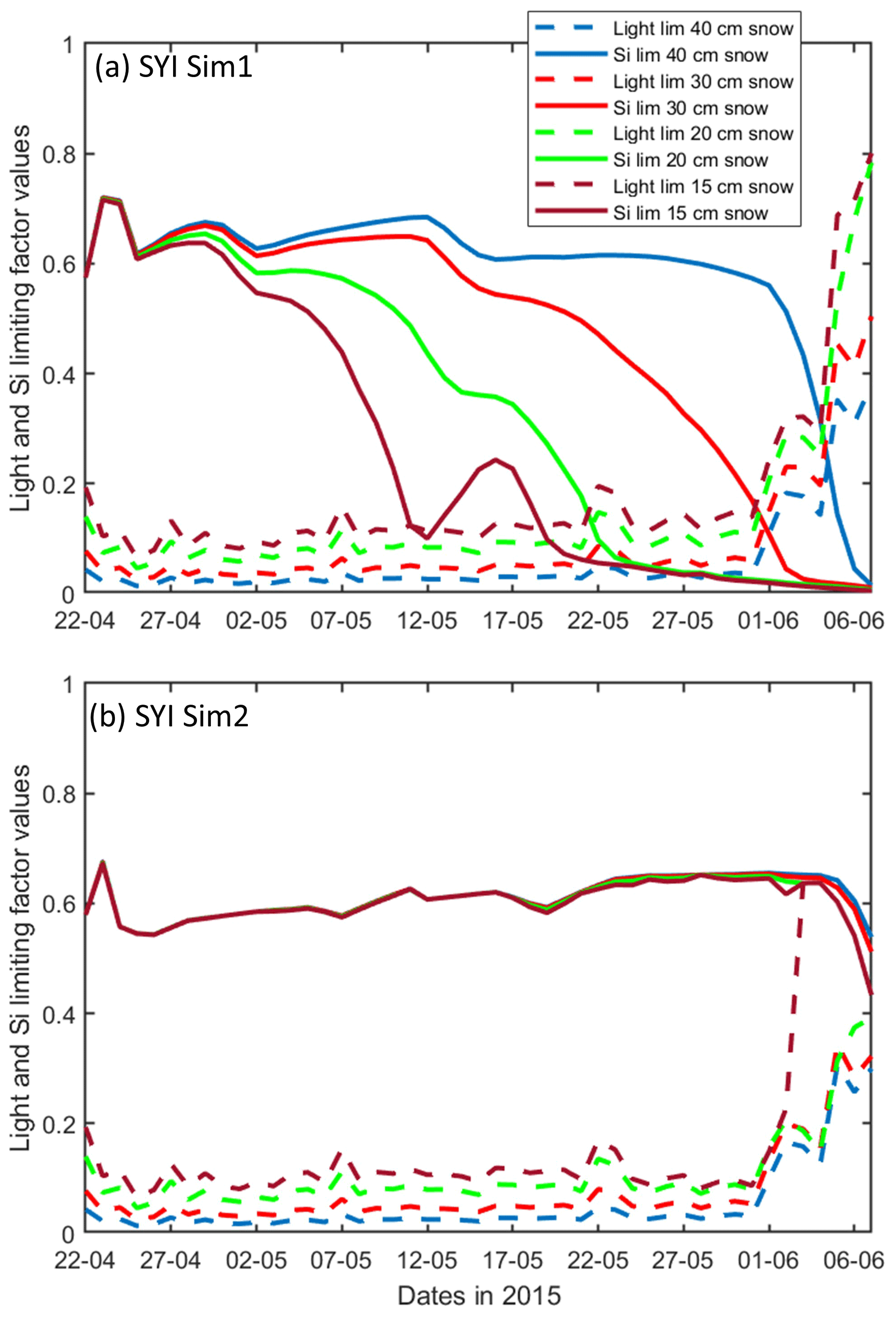
Figure 10Daily averaged results for the second-year ice (SYI) simulations 1 (a) and 2 (b), starting with a snow depth of 40 (default simulation), 30, 20, and 15 cm. Simulated evolution of light (dashed lines) and silicate (continuous lines) limitation (one means no limitation and zero is maximal limitation) are given as a function of time at the ice bottom layer (a value of 1 means no limitation). Refer to Table 1 for details about model simulations.
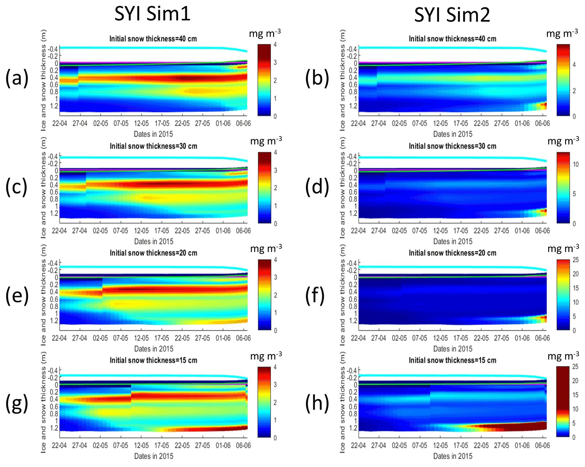
Figure 11Daily averaged results for second-year ice (SYI) simulations 1 (a, c, e, g) and 2 (b, d, f, h), starting with a snow depth of 40 (default simulation), 30, 20, and 15 cm. Simulated evolution of ice algae Chl a is given as a function of time and depth in the ice. The upper regions of the graphs above the green line with zero values are above the CICE biogrid and have no brine network. The magenta line represents sea level, and the cyan line represents the top of the snow layer. Refer to Table 1 for a description of model simulations.
SYI_Sim1 and 2 were repeated with varying snow thickness (Table 1 and Figs. 10 and 11). In the former simulation (Fig. 10a), as snow height decreases, there is a reduction in light limitation and a sharp increase in silicate limitation, overtaking light limitation (values becoming lower) as early as mid-May. In the latter simulation (Fig. 10b), light limitation prevails irrespective of snow height, except in the case of the lower snow height of 15 cm where silicate becomes more limiting towards the end of the simulation. With the decrease in snow height, there is an increase in Chl a concentration in all simulations. The highest values for SYI_Sim2 are around an order of magnitude larger than those for SYI_Sim1. Moreover, the decrease in snow heights is followed by an earlier and more intense bottom ice algal bloom.
The results obtained in this study support the initial hypothesis, showing that considering the role of velocity shear on turbulent nutrient exchanges between the ocean and the sea ice, formulated in a way consistent with heat exchanges, leads to a reduction in nutrient limitation that supports a significant increase in ice algal net primary production and Chl a biomass accumulation in the bottom ice layers, when production is nutrient limited. Therefore, our results are in line with empirical evidence provided by Cota et al. (1987) and Dalman et al. (2019), but to the best of our knowledge experimental evidence from properly designed experiments is still lacking to test our hypothesis. Moreover, our results do not imply necessarily that experiments carried out with other sea ice models would render the same trends. The implementation of turbulent mixing considerably relieved silicate limitation in the RL simulations, leading to an increase in NPP, the duration of the algal growth period, bottom Chl a concentration, and in-ice light absorption, increasing the light limitation due to shelf-shading (in the CICE model, optical ice properties are influenced by ice algal concentrations; Jeffery et al., 2016).
In the N-ICE2015 biogeochemical dataset (Assmy et al., 2016), the median of dissolved inorganic nitrogen to silicate ratios in all surface and subsurface water masses is above 1.7 (unpublished data), which is the upper limit for the nitrogen to silicate ratio for polar diatoms (e.g., Takeda, 1998; Krause et al., 2018). Therefore, it can be expected that silicate is more limiting than nitrogen for the production yields of the pennate diatoms characteristic of the bottom-ice communities in the region covered by the N-ICE2015 expedition (the dominant algal functional group in bottom ice, e.g., Leu et al., 2015; van Leeuwe et al., 2018). Elsewhere in the Arctic the opposite may be true, considering nitrate and silicate concentrations presented in Leu et al. (2015) and the number of process studies documenting such limitations (e.g., Campbell et al., 2016). However, the conclusions taken here about the effects of turbulent mixing are independent of the limiting nutrient.
Implementing turbulent diffusion between the ice and the ocean has obvious implications for model tuning. Our results for the RL show that with this formulation it was necessary to increase the half-saturation constant for silicate uptake and to reduce the ocean concentration of algal nitrogen (algalN), reducing the colonization of bottom ice by ice algae, to obtain Chl a values comparable to those observed (RL_Sim5). Therefore, whereas Duarte et al. (2017) had to reduce silicate limitation to improve the fit between modeled and observational data, the opposite approach was required when using turbulent diffusion in line with results reported in Lim et al. (2019) for Antarctic sea ice diatoms. This is an example of how one can get good model results via the wrong methods, which can have difficult to predict consequences on model forecasts under various scenarios.
In the SYI case, only a minor increase in bottom Chl a concentration was observed towards the end of simulations SYI_Sim_2 and SYI_Sim_3, when light limitation due to the thick snow cover was relieved by snow melt. Silicate limitation was not as severe as in SYI_Sim_1 due to greater bottom exchanges in the former simulations. The importance of snow cover in controlling ice algal phenology has been stressed before (e.g., Campbell et al., 2015; Leu et al., 2015).
Duarte et al. (2017) used the delta-Eddington parameter, corresponding to the standard deviation of the snow grain size (R_snow) (Urrego-Blanco et al., 2016), to tune model predicted shortwave radiation at the ice bottom. However, there was still a positive shortwave model bias in June. Therefore, our conclusion about the main limiting role of light in SYI is conservative. Moreover, there was no Chl a bottom maximum in part of SYI cores sampled during the N-ICE2015 expedition in the period covered by our simulations with an unusually high snow thickness (∼40 cm; Duarte et al., 2017; Olsen et al., 2017).
The dominant role of light limitation in SYI was confirmed in the simulations with reduced snow thickness and alleviated light limitation, with a bottom-ice algal Chl a maximum emerging earlier at snow thicknesses ≤20 cm. The reduction of snow thickness had a much larger effect in increasing Chl a concentration at the bottom layer when turbulent mixing was used due to lower silicate limitation. Reducing snow thickness led to a relatively early shift from light to silicate limitation when we used molecular and mixed-length diffusion, whereas this shift occurred only at the very end of the simulated period when we used turbulent diffusion at the ice–ocean interface driven by velocity shear instead of molecular diffusion. The effects of different types of diffusion upon reduction of the snow cover and the possible development of a bottom ice algal bloom are critical aspects when simulating ice algal phenology and attempting to quantify the contribution of sea ice algae to Arctic primary production.
Simulated shear-driven turbulent diffusivities are up to 4 orders of magnitude higher than molecular + mixed-length diffusivities at the bottom ice, and the results presented herein emphasize their potential role in sea ice biogeochemistry. The number and intensity of Arctic winter storms has increased over the 1979–2016 period (Rinke et al., 2017; Graham et al., 2017), and the effect of more frequent and more intensive winter storms in the Atlantic Sector of the Arctic Ocean is a thinner, weaker, and younger snow-laden ice pack (Graham et al., 2019). Storms that occur late in the winter season after a deep snowpack has accumulated have the potential to promote ice growth by dynamically opening leads where new ice growth can take place. The young ice of the refrozen leads does not have time to accumulate a deep snow layer until the melting season, which could lead to light limitation of algal growth. All things considered, it can be expected that ongoing trends in the Arctic will lead to a release from light limitation in increasingly larger areas of the ice pack in late winter, which will lead to more likely nutrient limitation earlier in spring (e.g., Lannuzel et al., 2020). These effects will be further amplified under thinning of the snowpack as observed in western Arctic and in the Beaufort and Chukchi seas over the last few decades (Webster et al., 2014). Therefore, properly parameterizing nutrient exchanges between the ice and the ocean in sea ice biogeochemical models is of utmost importance to avoid overestimating nutrient limitation and thus underestimating sea ice algal primary production.
In existing sea ice models there are “natural” differences between the way budgets for non-conservative tracers such as nutrients are closed compared to those of heat and salt, which are related to the biogeochemical sinks and sources (e.g., Eq. 18 in Vancoppenolle et al., 2010), but there are also some “inconsistencies” related to the way their transfers between the ocean and the ice are computed. Interestingly, some models (e.g., Jin et al., 2006, 2008; Hunke et al., 2015) apply the diffusion equation to calculate exchanges across the bottom ice to not only dissolved tracers but also algal cells. This is to guarantee a mechanism of ice colonization by microalgae. However, the usage of the same coefficient for dissolved and particulate components creates significant uncertainty.
Molecular diffusion is a slow process compared with turbulent exchanges. This justifies the usage of diffusion coefficients that are much higher than molecular diffusivity, as in Jin et al. (2006), using a value of m2 s−1, which is 4 orders of magnitude higher than the value indicated in Mann and Lazier (2005) ( m2 s−1), or the parameterization of molecular diffusivity as a function of friction velocity as in Mortenson et al. (2017). The approach proposed herein, formulating bottom-ice nutrient exchanges in a way that is consistent with heat exchanges, provides a physically sound, consistent, and easy to implement alternative.
Calculating diffusion fluxes across the molecular sublayer may be challenging, since it is necessary to estimate the boundary concentrations of this layer, which is only a few tenths of a millimeter thick (e.g., Lavoie et al., 2005). This implies resolving with a great detail the ocean surface layer (sensu MacPhee, 2008), which is not practical with standalone sea ice models but doable with coupled ocean–sea ice models. Moreover, one needs to know whether exchanges of heat, salt, and nutrients are dominated by molecular exchange or by turbulent exchange. This may be challenging on its own since it depends not only on knowing friction velocities but also on knowing the roughness of the bottom ice (e.g., Olsen et al., 2019). Ideally, when using coupled ocean–sea ice models (and assuming it is practical to estimate the type of dominant exchanges), one may use either the approach described by Lavoie et al. (2005) or the approach described herein based on McPhee (2008) and grounded on experimental work. Whatever the case, it seems rather likely that we still lack the measurements to properly evaluate these various approaches and find an optimal solution. The way forward implies the availability of eddy covariance data for 3D current velocity, temperature, salinity, and ideally a limiting nutrient collected at the sea ice–ocean interface over periods of sea ice growth and melting. Such data should be accompanied by vertical profiles for the same tracers at high resolution across the surface and the mixing layers (sensu McPhee, 2008) and by sea ice bottom samples. Such experiments may be carried out in the sea and in sea ice laboratories under controlled conditions, and they will help to evaluate the results presented herein and improve the parameterizations used in models for the sea ice–ocean interface. Another layer of complexity is the effects of sea ice ridges and keels on the turbulent exchange coefficients (Tsamados et al., 2014). According to these authors such effects are important for regional sea ice modeling, which reinforces the need for experimental studies of the type mentioned above.
Considering the role of velocity shear on turbulent nutrient exchanges at the interface between the ocean and the ice in a sea ice biogeochemical sub-model leads to a reduction in nutrient limitation and a significant increase in ice algal net primary production and Chl a biomass accumulation in the bottom-ice layers when production is nutrient limited. The results presented herein emphasize the potential role of bottom-ice nutrient exchange processes, irrespective of brine dynamics and other physical or chemical processes, in delivering nutrients to bottom-ice algal communities, and thus the importance of properly including them in sea ice models. The relevance of this becomes even more apparent considering ongoing changes in the Arctic icescape, with a predictable decrease in light limitation as ice becomes thinner and more fractured with an expected reduction in snow cover.
The software code used in this study may be found at https://doi.org/10.5281/zenodo.4675097 (Duarte, 2021b) and https://doi.org/10.5281/zenodo.4675021 (Duarte, 2021a).
This code is in a fork derived from the CICE Consortium repository (https://github.com/CICE-Consortium, last access: 26 January 2022).
The Consortium's code is open source with a standard three-clause BSD license and is under the following copyright license, available at (https://cice-consortium-cice.readthedocs.io/en/master/intro/copyright.html, last access: 27 January 2022).
Model forcing function files may be found at https://doi.org/10.5281/zenodo.4672176 (Duarte, 2021c). This includes data from Assmy et al. (2016, 2017), Gerland et al. (2017), Hudson et al. (2015, 2016) and Peterson et al. (2016).
Results from model simulations described above, in the form of CICE daily netCDF history files iceh.*, may be found at https://doi.org/10.5281/zenodo.4672210 (Duarte, 2021d).
There is one directory for each simulation, and it includes, in addition to the historical files, the input file (ice_in) with the simulation parameters.
The supplement related to this article is available online at: https://doi.org/10.5194/gmd-15-841-2022-supplement.
PD made the software changes, designed the experiments, performed the simulations, and prepared the manuscript with contributions from all co-authors. PA contributed to the writing of the manuscript. KC contributed to the writing of the manuscript. AS contributed to the writing of the manuscript and to funding acquisition.
The contact author has declared that neither they nor their co-authors have any competing interests.
Publisher's note: Copernicus Publications remains neutral with regard to jurisdictional claims in published maps and institutional affiliations.
This work has been supported by the Fram Centre Arctic Ocean flagship project “Mesoscale physical and biogeochemical modeling of the ocean and sea-ice in the Arctic Ocean” (project reference 66200), the Norwegian Metacenter for Computational Science application “NN9300K – Ecosystem modeling of the Arctic Ocean around Svalbard”, the Norwegian “Nansen Legacy” project (no. 276730), and the European Union's Horizon 2020 research and innovation programme under grant agreement no. 869154 (project FACE-IT). Contributions by Karley Campbell are supported by the Diatom ARCTIC project (NE/R012849/1;03F0810A), part of the Changing Arctic Ocean program, jointly funded by the UKRI Natural Environment Research Council and the German Federal Ministry of Education and Research (BMBF).
This paper was edited by Guy Munhoven and reviewed by Marcello Vichi and one anonymous referee.
Arrigo, K. R., Kremer, J. N., and Sullivan, C. W.: A Simulated Antarctic Fast Ice Ecosystem, J. Geophys. Res, 98, 6929–6946, 1993.
Assmy, P., Duarte, P., Dujardin, J., Fernández-Méndez, M., Fransson, A., Hodgson, R., Kauko, H., Kristiansen, S., Mundy, C. J., Olsen, L. M., Peeken, I., Sandbu, M., Wallenschus, J., and Wold, A.: N-ICE2015 water column biogeochemistry, Norwegian Polar Institute [data set], https://doi.org/10.21334/npolar.2016.3ebb7f64, 2016.
Assmy, P., Dodd, P. A., Duarte, P., Dujardin, J., Elliott, A., Fernández-Méndez, M., Fransson, A., Granskog, M. A., Hendry, K., Hodgson, R., Kauko, H., Kristiansen, S., Leng, M. J., Meyer, A., Mundy, C. J., Olsen, L. M., Peeken, I., Sandbu, M., Wallenschus, J., and Wold, A.: N-ICE2015 sea ice biogeochemistry, Norwegian Polar Institute [data set], https://doi.org/10.21334/npolar.2017.d3e93b31, 2017.
Brzezinski, M. A.: The Si-C-N Ratio of Marine Diatoms – Interspecific Variability and the Effect of Some Environmental Variables, J. Phycol., 21, 347–357, 1985.
Campbell, K., Mundy, C. J., Barber, D. G., and Gosselin, M.: Characterizing the sea ice algae chlorophyll a–snow depth relationship over Arctic spring melt using transmitted irradiance, J. Mar. Sys., 147, 76–84, https://doi.org/10.1016/j.jmarsys.2014.01.008, 2015.
Campbell, K., Mundy, C. J., Landy, J. C., Delaforge, A., Michel, C., and Rysgaard, S.: Community dynamics of bottom-ice algae in Dease Strait of the Canadian Arctic, Prog. Oceanogr., 149, 27–39, https://doi.org/10.1016/j.pocean.2016.10.005, 2016.
Carmack, E.: Circulation and Mixing in Ice-Covered Waters, in: The Geophysics of Sea Ice. NATO ASI Series (Series B: Physics), edited by: Untersteiner N. Springer, Boston, MA, 641–712, https://doi.org/10.1007/978-1-4899-5352-0_11, 1986.
Cota, G. F. and Horne, E. P. W.: Physical Control of Arctic Ice Algal Production, Mar. Ecol. Prog. Ser., 52, 111–121, https://doi.org/10.3354/meps052111, 1989.
Cota, G. F. and Sullivan, C. W.: Photoadaptation, Growth and Production of Bottom Ice Algae in the Antarctic, J. Phycol., 26, 399–411, https://doi.org/10.1111/j.0022-3646.1990.00399.x, 1990.
Cota, G. F., Prinsenberg, S. J., Bennett, E. B., Loder, J. W., Lewis, M. R., Anning, J. L., Watson, N. H. F., and Harris, L. R.: Nutrient Fluxes during Extended Blooms of Arctic Ice Algae, J. Geophys. Res.-Oceans, 92, 1951–1962, https://doi.org/10.1029/Jc092ic02p01951, 1987.
Dalman, L. A., Else, B. G. T., Barber, D., Carmack, E., Williams, W. J., Campbell, K. , Duke, P. J., Kirillov, S., and Mundy, C. J.: Enhanced bottom-ice algal biomass across a tidal strait in the Kitikmeot Sea of the Canadian Arctic, Elem. Sci. Anth., 7, 1–16, https://doi.org/10.1525/elementa.361, 2019.
Duarte, P.: CICE-Consortium/Icepack: Icepack with bottom drag, heat and nutrient turbulent diffusion (Version 1.1), Zenodo [code], https://doi.org/10.5281/zenodo.4675021, 2021a.
Duarte, P.: CICE-Consortium/CICE: CICE with bottom drag, heat and nutrient turbulent diffusion (Version 1.1), Zenodo [code], https://doi.org/10.5281/zenodo.4675097, 2021b.
Duarte, P.: The importance of turbulent ocean-sea ice nutrient exchanges for simulation of ice algal biomass and production with CICE6.1 and Icepack 1.2 – CICE forcing files (Version v1.0), Zenodo [data set], https://doi.org/10.5281/zenodo.4672176, 2021c.
Duarte, P.: The importance of turbulent ocean-sea ice nutrient exchanges for simulation of ice algal biomass and production with CICE6.1 and Icepack 1.2 – model simulations (Version v1.0), Zenodo [data set], https://doi.org/10.5281/zenodo.4672210, 2021d.
Duarte, P., Meyer, A., Olsen, L. M., Kauko, H. M., Assmy, P., Rosel, A., Itkin, P., Hudson, S. R., Granskog, M. A., Gerland, S., Sundfjord, A., Steen, H., Hop, H., Cohen, L., Peterson, A. K., Jeffery, N., Elliott, S. M., Hunke, E. C., and Turner, A. K.: Sea ice thermohaline dynamics and biogeochemistry in the Arctic Ocean: Empirical and model results, J. Geophys. Res.-Biogeo., 122, 1632–1654, https://doi.org/10.1002/2016JG003660, 2017.
Gerland, S., Granskog, M. A., King, J., and Rösel, A.: N-ICE2015 Ice core physics: temperature, salinity and density, Norwegian Polar Institute [data set], https://doi.org/10.21334/npolar.2017.c3db82e3, 2017.
Gosselin, M., Legendre, L., Demers, S., and Ingram, R. G.: Responses of Sea-Ice Microalgae to Climatic and Fortnightly Tidal Energy Inputs (Manitounuk Sound, Hudson-Bay), Can. J. Fish. Aquat. Sci., 42, 999–1006, https://doi.org/10.1139/f85-125, 1985.
Graham, R. M., Rinke, A., Cohen, L., Hudson, S. R., Walden, V. P., Granskog, M. A., Dorn, W., Kayser, M., and Maturilli, M.: A comparison of the two Arctic atmospheric winter states observed during N-ICE2015 and SHEBA, J. Geophys. Res.-Atmos., 122, 5716–5737, https://doi.org/10.1002/2016JD025475, 2017.
Graham, R. M., Itkin, P., Meyer, A., Sundfjord, A., Spreen, G., Smedsrud, L. H., Liston, G. E., Cheng, B., Cohen, L., Divine, D., Fer, I., Fransson, A., Gerland, S., Haapala, J., Hudson, S. R., Johansson, A. M., King, J., Merkouriadi, I., Peterson, A. K., Provost, C., Randelhoff, A., Rinke, A., Rosel, A., Sennechael, N., Walden, V., Duarte, P., Assmy, P., Steen, H., and Granskog, M. A.: Winter storms accelerate the demise of sea ice in the Atlantic sector of the Arctic Ocean, Sci. Rep.-UK, 9, 9222, https://doi.org/10.1038/S41598-019-45574-5, 2019.
Granskog, M. A., Fer, I., Rinke, A., and Steen, H.: Atmosphere-Ice-Ocean-Ecosystem Processes in a Thinner Arctic Sea Ice Regime: The Norwegian Young Sea ICE (N-ICE2015) Expedition, J. Geophys. Res.-Oceans, 123, 1586–1594, https://doi.org/10.1002/2017jc013328, 2018.
Hegseth, E. N.: Sub-Ice Algal Assemblages of the Barents Sea – Species Composition, Chemical-Composition, and Growth-Rates, Polar. Biol., 12, 485–496, 1992.
Hudson, S. R., Cohen, L., and Walden, V.: N-ICE2015 surface meteorology, Norwegian Polar Institute [data set], https://doi.org/10.21334/npolar.2015.056a61d1, 2015.
Hudson, S. R., Cohen, L., and Walden, V.: N-ICE2015 surface broadband radiation data, Norwegian Polar Institute [data set], https://doi.org/10.21334/npolar.2016.a89cb766, 2016.
Hunke, E. C., Lipscomb, W. H., Turner, A. K., Jeffery, N., and Elliot, S.: CICE: the Los Alamos Sea Ice Model. Documentation and User's Manual Version 5.1, Los Alamos National Laboratory, USA, LA-CC-06-012, 2015.
Ingram, R. G., Osler, J. C., and Legendre, L.: Influence of Internal Wave-Induced Vertical Mixing on Ice Algal Production in a Highly Stratified Sound, Estuar. Coast. Shelf. S., 29, 435–446, https://doi.org/10.1016/0272-7714(89)90078-4, 1989.
Jeffery, N., Hunke, E. C., and Elliott, S. M.: Modeling the transport of passive tracers in sea ice, J. Geophys. Res.-Oceans, 116, C07020, https://doi.org/10.1029/2010jc006527, 2011.
Jeffery, N., Elliott, S., Hunke, E. C., Lipscomb, W. H., and Turner, A. K.: Biogeochemistry of CICE: The Los Alamos Sea Ice Model, Documentation and User's Manual,Zbgc_colpkg modifications to Version 5, Los Alamos National Laboratory, Los Alamos, NM, 2016.
Jin, M., Deal, C. J., Wang, J., Shin, K. H., Tanaka, N., Whitledge, T. E., Lee, S. H., and Gradinger, R. R.: Controls of the landfast ice–ocean ecosystem offshore Barrow, Alaska, Ann. Glaciol., 44, 63–72, 2006.
Jin, M., Deal, C., and Jia, W.: A coupled ice-ocean ecosystem model for I-D and 3-D applications in the Bering and Chukchi Seas, Chinese Journal of Polar Science, 19, 218–229, 2008.
Krause, J. W., Duarte, C. M., Marquez, I. A., Assmy, P., Fernández-Méndez, M., Wiedmann, I., Wassmann, P., Kristiansen, S., and Agustí, S.: Biogenic silica production and diatom dynamics in the Svalbard region during spring, Biogeosciences, 15, 6503–6517, https://doi.org/10.5194/bg-15-6503-2018, 2018.
Lake, R. A. and Lewis, E. L.: Salt rejection by sea ice during growth, J. Geophys. Res., 75, 583–597, 1970.
Lannuzel, D., Tedesco, T., van Leeuwe, M., Campbell, K., Flores, H., Delille, B., Miller, L., Stefels, J., Assmy, P., Bowman, J., Brown, K., Castellani, G., Chierici, M., Crabeck, O., Damm, E., Else, B., Fransson, A., Fripiat, F., Geilfus, N. X., Jacques, C., Jones, E., Kaartokallio, H., Kotovitch, M., Meiners, K., Moreau, S., Nomura, D., Peeken, I., Rintala, J. M., Steiner, N., Tison, J. L., Vancoppenolle, M., Van der Linden, F., Vichi, M., and Wongpan, P.: The future of Arctic sea-ice biogeochemistry and ice-associated ecosystems, Nat. Clim. Change, 10, 983–992, https://doi.org/10.1038/s41558-020-00940-4, 2020.
Lavoie, D., Denman, K., and Michel, C.: Modeling ice algal growth and decline in a seasonally ice-covered region of the Arctic (Resolute Passage, Canadian Archipelago), J. Geophys. Res.-Oceans, 110, C11009, https://doi.org/10.1029/2005jc002922, 2005.
Leu, E., Mundy, C. J., Assmy, P., Campbell, K., Gabrielsen, T. M., Gosselin, M., Juul-Pedersen, T., and Gradinger, R.: Arctic spring awakening – Steering principles behind the phenology of vernal ice algal blooms, Progr. Oceanogr., 139, 151–170, https://doi.org/10.1016/j.pocean.2015.07.012, 2015.
Lim, S. M., Moreau, S., Vancoppenolle, M., Deman, F., Roukaerts, A., Meiners, K. M., Janssens, J., and Lannuzel, D.: Field Observations and Physical-Biogeochemical Modeling Suggest Low Silicon Affinity for Antarctic Fast Ice Diatoms, J. Geophys. Res.-Oceans, 124, 7837–7853, https://doi.org/10.1029/2018jc014458, 2019.
Mann, K. H. and Lazier, J. R. N.: Dynamics of Marine Ecosystems, Third Edition, Blackwell Publishing Ltd., Carlton, Victoria 3053, Australia, 503 pp., https://doi.org/10.1002/9781118687901, 2005.
McPhee, M.: Air-ice-ocean interaction: Turbulent ocean boundary layer exchange processes. Springer-Verlag, New York, 216 pp., https://doi.org/10.1007/978-0-387-78335-2, 2008.
McPhee, M. G., Morison, J. H., and Nilsen, F.: Revisiting heat and salt exchange at the ice-ocean interface: Ocean flux and modeling considerations, J. Geophys. Res.-Oceans, 113, C06014, https://doi.org/10.1029/2007jc004383, 2008.
Mortenson, E., Hayashida, H., Steiner, N., Monahan, A., Blais, M., Gale, M. A., Galindo, V., Gosselin, M., Hu, X. M., Lavoie, D., and Mundy, C. J.: A model-based analysis of physical and biological controls on ice algal and pelagic primary production in Resolute Passage, Elem. Sci. Anth., 5, 39, https://doi.org/10.1525/Elementa.229, 2017.
Nelson, D. M. and Treguer, P.: Role of Silicon as a Limiting Nutrient to Antarctic Diatoms – Evidence from Kinetic-Studies in the Ross Sea Ice-Edge Zone, Mar. Ecol. Prog. Ser., 80, 255–264, https://doi.org/10.3354/meps080255, 1992.
Niedrauer, T. M. and Martin, S.: Experimental-Study of Brine Drainage and Convection in Young Sea Ice, J. Geophys. Res.-Oceans, 84, 1176–1186, https://doi.org/10.1029/JC084iC03p01176, 1979.
Notz, D. and Worster, M. G.: Desalination processes of sea ice revisited, J. Geophys. Res.-Oceans, 114, C05006, https://doi.org/10.1029/2008jc004885, 2009.
Olsen, L. M., Laney, S. R., Duarte, P., Kauko, H. M., Fernández-Méndez, M., Mundy, C. J., Rösel, A., Meyer, A., Itkin, P., Cohen, L., Peeken, I., Tatarek, A., Róźańska, M., Wiktor, J., Taskjelle, T., Pavlov, A. K., Hudson, S. R., Granskog, M. A., Hop, H., and Assmy, P.: The seeding of ice-algal blooms in Arctic pack ice: the multiyear ice seed repository hypothesis, J. Geophys. Res.-Biogeo., 122, 1529–1548, https://doi.org/10.1002/2016jg003668, 2017.
Olsen, L. M., Duarte, P., Peralta-Ferriz, C., Kauko, H. M., Johansson, M., Peeken, I., Różańska-Pluta, M., Tatarek, A., Wiktor, J., Fernández-Méndez, M., Wagner, P. M., Pavlov, A. K., Hop, H., and Assmy, P.: A red tide in the pack ice of the Arctic Ocean, Sci. Rep.-UK, 9, 9536, https://doi.org/10.1038/s41598-019-45935-0, 2019.
Peterson, A. K., Fer, I., Randelhoff, A., Meyer, A., Håvik, L., Smedsrud, L. H., Onarheim, L., Muilwijk, M., Sundfjord, A., and McPhee, M. G.: N-ICE2015 Ocean turbulent fluxes from under-ice turbulence cluster (TIC), Norwegian Polar Institute [data set], https://doi.org/10.21334/npolar.2016.ab29f1e2, 2016.
Reeburgh, W. S.: Fluxes Associated with Brine Motion in Growing Sea Ice, Polar Biol., 3, 29–33, https://doi.org/10.1007/Bf00265564, 1984.
Rinke, A., Maturilli, M., Graham, R. M., Matthes, H., Handorf, D., Cohen, L., Hudson, S. R., and Moore, J. C.: Extreme cyclone events in the Arctic: Wintertime variability and trends, Environ. Res. Lett., 12, 094006, https://doi.org/10.1088/1748-9326/Aa7def, 2017.
Smith, R. E. H., Cavaletto, J. F., Eadie, B. J., and Gardner, W. S.: Growth and Lipid-Composition of High Arctic Ice Algae during the Spring Bloom at Resolute, Northwest-Territories, Canada, Mar. Ecol. Prog. Ser., 97, 19–29, https://doi.org/10.3354/meps097019, 1993.
Takeda, S.: Influence of iron availability on nutrient consumption ratio of diatoms in oceanic waters, Nature, 393, 774–777, https://doi.org/10.1038/31674, 1998.
Tedesco, L. and Vichi, M.: BFM-SI: a new implementation of the Biogeochemical Flux Model in sea ice. in: CMCC Research Papers, available at: http://hdl.handle.net/2122/5956 (last access: 27 January 2022), 2010.
Tedesco, L., Vichi, M., and Scoccimarro, E.: Sea-ice algal phenology in a warmer Arctic, Sci. Adv., 5, eaav4830, https://doi.org/10.1126/sciadv.aav4830, 2019.
Thomas, M., Vancoppenolle, M., France, J. L., Sturges, W. T., Bakker, D. C. E., Kaiser, J., and von Glasow, R.: Tracer Measurements in Growing Sea Ice Support Convective Gravity Drainage Parameterizations, J. Geophys. Res.-Oceans, 125, e2019JC015791, https://doi.org/10.1029/2019JC015791, 2020.
Tsamados, M., Feltham, D. L., Schroeder, D., Flocco, D., Farrell, S. L., Kurtz, N., Laxon, S. W., and Bacon, S.: Impact of Variable Atmospheric and Oceanic Form Drag on Simulations of Arctic Sea Ice, J. Phys. Oceanogr., 44, 1329–1353, https://doi.org/10.1175/Jpo-D-13-0215.1, 2014.
Turner, A. K., Hunke, E. C., and Bitz, C. M.: Two modes of sea-ice gravity drainage: A parameterization for large-scale modeling, J. Geophys. Res.-Oceans, 118, 2279–2294, https://doi.org/10.1002/jgrc.20171, 2013.
Urrego-Blanco, J. R., Urban, N. M., Hunke, E. C., Turner, A. K., and Jeffery, N.: Uncertainty quantification and global sensitivity analysis of the Los Alamos sea ice model, J. Geophys. Res.-Oceans, 121, 2709–2732, https://doi.org/10.1002/2015JC011558, 2016.
Vancoppenolle, M., Bitz, C. M., and Fichefet, T.: Summer landfast sea ice desalination at Point Barrow, Alaska: Modeling and observations, J. Geophys. Res.-Oceans, 112, C04022, https://doi.org/10.1029/2006jc003493, 2007.
Vancoppenolle, M., Goosse, H., de Montety, A., Fichefet, T., Tremblay, B., and Tison, J. L.: Modeling brine and nutrient dynamics in Antarctic sea ice: The case of dissolved silica, J. Geophys. Res.-Oceans, 115, C02005, https://doi.org/10.1029/2009jc005369, 2010.
Vancoppenolle, M., Bopp, L., Madec, G., Dunne, J., Ilyina, T., Halloran, P. R., and Steiner, N.: Future Arctic Ocean primary productivity from CMIP5 simulations: Uncertain outcome, but consistent mechanisms, Global Biogeochem. Cy., 27, 605–619, https://doi.org/10.1002/gbc.20055, 2013.
van Leeuwe, M. A., Tedesco, L., Arrigo, K. R., Assmy, P., Campbell, K., Meiners, K. M., Rintala, J. M., Selz, V., Thomas, D. N., and Stefels, J.: Microalgal community structure and primary production in Arctic and Antarctic sea ice: A synthesis, Elem. Sci. Anth., 6, 4, https://doi.org/10.1525/elementa.267, 2018.
Wakatsuchi, M. and Ono, N.: Measurements of Salinity and Volume of Brine Excluded from Growing Sea Ice, J. Geophys. Res.-Oceans, 88, 2943–2951, https://doi.org/10.1029/JC088iC05p02943, 1983.
Webster, M. A., Rigor, I. G., Nghiem, S. V., Kurtz, N. T., Farrell, S. L., Perovich, D. K., and Sturm, M.: Interdecadal changes in snow depth on Arctic sea ice, J. Geophys. Res.-Oceans, 119, 5395–5406, https://doi.org/10.1002/2014JC009985, 2014.
Wells, A. J., Wettlaufer, J. S., and Orszag, S. A.: Brine fluxes from growing sea ice, Geophys. Res. Lett., 38, L04501, https://doi.org/10.1029/2010gl046288, 2011.