the Creative Commons Attribution 4.0 License.
the Creative Commons Attribution 4.0 License.
 | 18 Nov 2022
A local particle filter and its Gaussian mixture extension implemented with minor modifications to the LETKF
Shunji Kotsuki
Takemasa Miyoshi
Keiichi Kondo
Roland Potthast
A particle filter (PF) is an ensemble data assimilation method that does not assume Gaussian error distributions. Recent studies proposed local PFs (LPFs), which use localization, as in the ensemble Kalman filter, to apply the PF efficiently for high-dimensional dynamics. Among others, Penny and Miyoshi (2016) developed an LPF in the form of the ensemble transform matrix of the local ensemble transform Kalman filter (LETKF). The LETKF has been widely accepted for various geophysical systems, including numerical weather prediction (NWP) models. Therefore, implementing the LPF consistently with an existing LETKF code is useful.
This study develops a software platform for the LPF and its Gaussian mixture extension (LPFGM) by making slight modifications to the LETKF code with a simplified global climate model known as Simplified Parameterizations, Primitive Equation Dynamics (SPEEDY). A series of idealized twin experiments were accomplished under the ideal-model assumption. With large inflation by the relaxation to prior spread, the LPF showed stable filter performance with dense observations but became unstable with sparse observations. The LPFGM showed a more accurate and stable performance than the LPF with both dense and sparse observations. In addition to the relaxation parameter, regulating the resampling frequency and the amplitude of Gaussian kernels was important for the LPFGM. With a spatially inhomogeneous observing network, the LPFGM was superior to the LETKF in sparsely observed regions, where the background ensemble spread and non-Gaussianity were larger. The SPEEDY-based LETKF, LPF, and LPFGM systems are available as open-source software on GitHub (https://github.com/skotsuki/speedy-lpf, last access: 16 November 2022) and can be adapted to various models relatively easily, as in the case of the LETKF.
- Article
(6341 KB) - Full-text XML
- BibTeX
- EndNote


Ensemble-based data assimilation (DA) has been broadly applied in geoscience fields such as weather and ocean prediction. The ensemble Kalman filter (EnKF) has been intensely investigated for the past two decades, such as for the perturbed observation method (Evensen, 1994; Burgers et al., 1998; Houtekamer and Mitchel, 1998; van Leeuwen, 2020) and for ensemble square root filters (e.g., Anderson, 2001; Bishop et al., 2001; Whitaker and Hamill, 2002; Hunt et al., 2007). The advantages of the EnKF are in its flow-dependent error estimates, represented by an ensemble, and in its relative ease of implementation in nonlinear dynamical systems, such as numerical weather prediction (NWP) models. The degrees of freedom of dynamical models (e.g., >O(108) for NWP models) are much larger than the typically affordable ensemble size (<O(103)). On the other hand, atmospheric and oceanic models show local low dimensionality (Patil et al., 2001; Oczkowski et al., 2005), and practical EnKF implementations use a localization technique that limits the impact of distant observations while also reducing the effective degrees of freedom. Among various kinds of EnKFs, the local ensemble transform Kalman filter (LETKF; Hunt et al., 2007) is widely utilized in operational NWP centers in the same manner, such as the Deutscher Wetterdienst (DWD) and the Japan Meteorological Agency (JMA). Analysis updates of the LETKF are performed by multiplying the ensemble transform matrix to the prior ensemble perturbation matrix, following the ensemble transform Kalman filter (ETKF, Bishop et al., 2001; Wang et al., 2004).
The particle filter (PF) is another ensemble DA method broadly applicable to nonlinear and non-Gaussian problems (see van Leeuwen, 2009, and van Leeuwen et al., 2019, for reviews on geoscience applications). The PF potentially solves some issues in the basic assumptions of the EnKF by permitting nonlinear observation operators and non-Gaussian likelihood functions (Penny and Miyoshi, 2016). For example, assimilating precipitation observations with a standard EnKF is difficult, partly because of their non-Gaussian errors (Lien et al., 2013, 2016; Kotsuki et al., 2017a). The PF can treat such variables with non-Gaussian errors properly. Several PF methods have been explored for low-dimensional problems in early studies (Gordon et al., 1993; van Leeuwen, 2009). However, applying the PF to high-dimensional dynamical systems is generally difficult, because the number of particles or the ensemble size must be increased exponentially with the system size to avoid a weight collapse in which very few particles occupy most of the weights (Snyder et al., 2008, 2015). If a weight collapse occurs, the PF loses the diversity of the particles after resampling. Therefore, we need to assure that the weights are similarly distributed among particles. Previous studies developed the equivalent-weights particle filter (EWPF; van Leeuwen, 2010; Ades and van Leeuwen, 2013, 2015; Zhu et al., 2016) to extend time until a weight collapse by using the proposal density to drive the particles toward the high-probability region of the posterior. However, even PFs with proposal densities are unable to prevent the weights from collapsing.
Alternatively, the local particle filter (LPF) uses localization to avoid a weight collapse by limiting the impact of observations within a local domain. Localization is a well-adopted method for the EnKF to treat sampling errors due to a limited ensemble size. Several LPFs have been proposed to apply the PF efficiently to high-dimensional systems (e.g., Bengtsson et al., 2003; van Leeuwen, 2009; Poterjoy, 2016; Penny and Miyoshi, 2016; Poterjoy and Anderson, 2016; Farchi and Bocquet, 2018; van Leeuwen et al., 2019). Among them, Penny and Miyoshi (2016) developed an LPF by means of the ensemble transform matrix of the LETKF. The LETKF has been commonly used for diverse geophysical systems, and consistent implementation with an available LETKF code would be useful. The DWD implemented the LPF in an operational global model based on the operational LETKF code and described stable performance in the operational setting (Potthast et al., 2019). Walter and Potthast (2022; hereafter WP22) extended the LPF to the Gaussian mixture for further improvements.
The goal of this study is to develop and provide a software platform to accelerate research on LPF and its Gaussian mixture extension (hereafter, LPFGM). Although many studies on LPF have used simple idealized chaotic models, such as the 40-variable Lorenz model (hereafter, “L96”; Lorenz, 1996; Lorenz and Emanuel, 1998), the present study uses a simplified atmospheric general circulation model, defined as the Simplified Parameterizations, Primitive Equation Dynamics (SPEEDY) model (Molteni, 2003). Miyoshi (2005) coupled the LETKF with the SPEEDY model for the first time. This study extends the SPEEDY-LETKF code and implements the LPF and LPFGM. As demonstrated below, the LPF and LPFGM can be implemented easily, with simple modifications to the existing LETKF code.
The remainder of this paper is organized as follows. Section 2 explains the mathematical formulation of the LETKF, LPF, and LPFGM, followed by a description of the specific modifications made to the existing LETKF code. Section 3 presents the experimental settings. Section 4 outlines the results and discussions. Lastly, Sect. 5 provides a summary.
2.1 Local ensemble transform Kalman filter
Hunt et al. (2007) introduced the LETKF as a computationally efficient EnKF by combining the local ensemble Kalman filter (Ott et al., 2004) and ETKF (Bishop et al., 2001). Let Xt be a matrix composed of m ensemble state vectors. The ensemble mean vector and perturbation matrix of Xt are given by (∈ℝn) and ( respectively, where n is the system size. The subscript t indicates the time, and the superscript (i) denotes the ith ensemble member. The analysis equations of the LETKF are specified by
where 1 is a row vector whose elements are all 1 (∈ℝm); T is the ensemble transform matrix (); is the error covariance matrix in the ensemble space (); Y≡HZ is the ensemble perturbation matrix in the observation space (); R is the observation error covariance matrix (); y is the observation vector (∈ℝp); H is the linear observation operator matrix (); and H is the observation operator that may be nonlinear. Here, p is the number of observations. The superscripts “o”, “b”, and “a” denote the observation, background (prior), and analysis (posterior), respectively. The matrix TLETKF denotes the ensemble transform matrix of the LETKF. The first and second terms on the right-hand side of Eq. (2) correspond to the updates of ensemble mean and perturbation, respectively. The ETKF computes the analysis error covariance matrix in the ensemble space by
where β is a multiplicative inflation factor. Equations (1) and (2) are derived from the Kalman filter equations, given by
where K is the Kalman gain (), and P is the error covariance matrix in the model space (). Derivations of Eqs. (5) and (6) are detailed in Appendix A. The EnKF approximates the error covariance matrix by . Hunt et al. (2007) provide more details on deriving Eqs. (1) and (2) from the Kalman filter equations. For nonlinear observation operators, the following approximation is used:
The LETKF provides and of Eq. (2) by solving the eigenvalue decomposition of , where U is a square matrix () composed of eigenvectors, and Λ is a diagonal matrix () composed of the corresponding eigenvalues. The eigenvalue decomposition leads to and .
The localization is practically important for mitigating sampling errors in the ensemble-based error covariance with a limited ensemble size (Houtekamer and Zhang, 2016). With localization, the LETKF computes the transform matrix TLETKF at every model grid point independently by assimilating a subset of observations within the localization cut-off radius. The LETKF employs localization by inflating the observation error variance so that observations distant from the analysis model grid point have fewer impacts (Hunt et al., 2007; Miyoshi and Yamane, 2007).
For local analysis schemes, a spatially smooth transition of the transform matrix TLETKF is essential to prevent abrupt changes in the analyses of neighboring grid points. The LETKF realizes a smooth transition of the transform matrix by using the symmetric square root of (Hunt et al., 2007). The symmetric square root matrix minimizes the mean-square distance between identity matrix I and ; therefore, the analysis ensemble perturbations can be closer to the background ensemble perturbation.
The EnKF generally underestimates the error variance, mainly because of model errors, nonlinear dynamics, and limited ensemble size. Therefore, a covariance inflation technique is used to inflate the underestimated error variance (Houtekamer and Mitchell, 1998). Among several kinds of covariance inflations methods, the present study considers multiplicative inflation (Anderson and Anderson, 1999) and relaxation to the prior scheme (Zhang et al., 2004), as implemented by Whitaker and Hamill (2012). In multiplicative inflation, the ensemble-based covariance is multiplied by a factor β (Pb→βPb). This multiplicative inflation is employed in Eq. (3) in the LETKF. In this study, the LETKF experiments use the approach of Miyoshi (2011), which adaptively estimates a spatially varying inflation factor on the basis of the innovation statistics of Desroziers et al. (2005). In realistic problems, covariance relaxation methods are often used to inflate the posterior perturbation (e.g., Terasaki et al., 2019; Kotsuki et al., 2019b). This study utilizes the relaxation to prior spread (RTPS; Whitaker and Hamill, 2012), given by
where α is the RTPS parameter, and σ is the ensemble spread. The subscript (k) denotes the kth model variable or the kth component of the state vector. Although this study only uses multiplicative inflation for the LETKF experiments, the posterior error perturbation is inflated by RTPS for LPF and LPFGM.
2.2 Local particle filter with ensemble transform matrix
Here, we describe the LPF in the form of the ensemble transform matrix of the LETKF (Reich, 2013; Penny and Miyoshi, 2016; Potthast et al., 2019). The PF is a direct Monte Carlo realization of Bayes' theorem, given by
where is the probability of state x given all observations yo up to time t. The PF approximates the prior probability density function (PDF), which appears in the numerator of Eq. (9), using an ensemble forecast
where δ is the Dirac's delta function, and wb(i) is the prior weight of the ith particle (i.e., ensemble member) at the previous analysis time. If particles are resampled at the previous analysis time, all particles have the same weight . The sum of the weights is always 1. The denominator on the right-hand side of Eq. (9) can be estimated by
This study assumes a Gaussian likelihood function, given by
This assumption means the observation error distribution is assumed to be Gaussian. Then, the posterior can be expressed by
where q is the likelihood. Equation (14) results in posterior weights that satisfy .
To mitigate weight collapse, the local PF (LPF) solves the PF equations by assimilating local observations surrounding the analysis grid point. This study uses Penny and Miyoshi's (2016) approach that computes the analysis at every model grid point independently, with the observation error covariance R being inflated by the inverse of a localization function, as in the LETKF (Penny and Miyoshi, 2016).
Sampling importance resampling (SIR) is a technique for applying the PF for high-dimensional dynamics with a limited amount of particles. The resampling process rearranges the particles to effectively represent the densest areas of the posterior PDF. After resampling, each particle has equal weights, and the posterior PDF is given by
The resampling process can be expressed as equally valid to the ensemble transform matrix of the ETKF (Reich, 2013; Penny and Miyoshi, 2016), given by
where TLPF denotes the ensemble transform matrix of the LPF. Here, we applied based on the following necessary condition of the ensemble transform matrix for the LPF:
In addition to Eq. (18), the ideal resampling matrix satisfies the following two conditions:
-
-
spatially smooth transition of Tt,LPF,
where m is the ensemble size, and T(i,j) indicates the ith-row and jth-column element of the matrix T.
The resampling matrix significantly affects the filter performance (Farchi and Bocquet, 2018). The present study constructs resampling matrices based on the Monte Carlo approach. This resampling method uses m random numbers r(i) () drawn from uniform distribution U ([0,1]) and accumulated weights wt,acc:
By definition, is 1. After sorting r to be the ascending order rsorted, we generate the resampling matrix using Algorithm 1. This procedure is similar to the resampling of Potthast et al. (2019), but it employs an additional treatment so that the resampling matrix is close to the identity matrix (line 10 of Algorithm 1; Fig. 1b and c).
Algorithm 1Generation of the resampling matrix T.
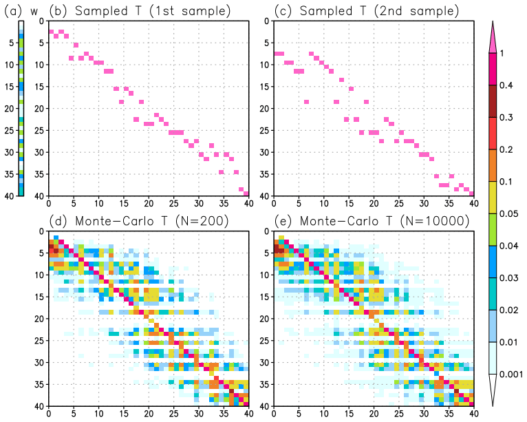
Figure 1Examples of the resampling matrix in the case of 40 particles with a given weight generated by uniform random numbers. (a) Weight for 40 particles. (b, c) Examples of sampled resampling matrices by Algorithm 1 using different random numbers r. (d, e) Resampling matrices using the Monte Carlo stochastic approach with 200 and 10 000 sampled matrices, respectively.
Classical resampling can produce the same particles, resulting in the loss of diversity of posterior particles. Therefore, additional treatments are required to generate slightly different posterior particles. Potthast et al. (2019) proposed adding Gaussian random noise to Tt,LPF to prevent the generation of the same particles. As an alternative, the present study uses the Monte Carlo approach that repeats Algorithm 1 many times with different random numbers and takes the average of the generated resampling matrices (Fig. 1). Using different random numbers r, the resampling matrices differ (Fig. 1b and c), even if the same weight is used (Fig. 1a). By averaging the resampling matrices generated by using different random numbers, we get matrices that have higher weights in the diagonal components and lower weights in the off-diagonal components (Fig. 1d and e). The Monte Carlo approach makes the resampling matrix closer to the identity matrix, which is beneficial for a smooth transition in space. In addition, this stochastic approach approximates Eq. (19) using the Monte Carlo approach. The generated transform matrix with 200 samples (Fig. 1c) is close to that with 10 000 samples (Fig. 1d) in the case of 40 particles. Therefore, the transform matrices are generated by averaging 200 sampled matrices in subsequent LPF experiments. Hereafter, we call this resampling method “MC resampling”, which is used in the following experiments. The number of required samples for MC resampling is briefly investigated in Appendix B.
The effective particle (or ensemble) size Neff (Kong et al., 1994) is useful to measure the diversity of particles in LPF:
If Neff is sufficiently large (Neff≈m), no resampling is needed. This study considers a tunable parameter N0 as a criterion for resampling:
Without resampling (), the posterior weight is succeeded for the subsequent forecast as follows:
where τ is the tunable forgetting factor . Here, τ=1 means the subsequent prior weight has the same weights , whereas the posterior weight is completely succeeded to when τ=0. This weight succession (Eq. 23) can be interpreted as a temporal localization that reduces the impact of observations temporally distant from the assimilation time. The weight succession in local PF is not trivial, because the weight (or likelihood) of particles would move with the dynamical flow. Similar discussions can be found for the advection of localization functions (e.g., Ota et al., 2013; Kotsuki et al., 2019a). This study assumes no flow motion of the weights and simply uses Eq. (23) at each grid point independently.
Although the LETKF applies inflation to the prior error covariance (i.e., Pb→βPb), this inflation is suboptimal to the LPF, partly because the weight collapse occurs more easily if multiplicative inflation is applied to the prior perturbation (see Eq. 15). Therefore, the LPF usually applies inflation to the posterior particles (e.g., Penny and Miyoshi, 2016; Farchi and Bocquet, 2018). The present study uses the RTPS to inflate posterior perturbations for the LPF. We do not use the RTPS for the LETKF experiments, since the Miyoshi (2011) adaptive multiplicative inflation is known to outperform the manually tuned RTPS for idealized twin experiments with SPEEDY, based on the authors' preliminary experiments and Yoichiro Ota (personal communication, 2021).
Preliminary experiments showed that the RTPS outperformed the relaxation to prior perturbation (RTPP; Zhang et al., 2004) for the LPF. Having some noise in the transform matrix is important for the LPF to maintain the diversity of posterior particles. The RTPP makes the transform matrix closer to the identity matrix, resulting in less diverged posterior particles. Therefore, the RTPS would be a more suitable relaxation method than the RTPP for LPF.
2.3 LPF with Gaussian mixture extension
For the LPF to avoid weight collapse, assimilating too many independent observations in the local area is not desirable (van Leeuwen et al., 2019). To solve this problem, hybrid algorithms of EnKF and PF have been explored to efficiently assimilate massive observation data. The Gaussian mixture extension of the LPF is one such hybrid algorithm (Hoteit et al., 2008; Stordal et al., 2011; WP22). In the Gaussian mixture extension, the prior PDF is approximated by a combination of Gaussian distributions centered at the values of the particles, given by:
where is the Gaussian kernel, with mean and covariance . Here, hat indicates matrices for the Gaussian kernels (e.g., prior error covariance , observation error covariance , and Kalman gain . The covariance of the Gaussian kernel uses the sampled covariance matrix , such that
where γ (>0) is a tunable parameter that regulates the amplitude and width of the Gaussian kernel (i.e., uncertainty of particles). For example, larger γ reduces amplitude and increases the width of the Gaussian kernel. Because the kernel is supposed to have a Gaussian distribution, increasing the Gaussian kernel's width results in a decrease in amplitude. The LPFGM results in the same analysis of the LPF when γ is 0 (γ→0).
The Gaussian mixture performs a two-step update to obtain the posterior particles. The first update moves the center of the Gaussian kernel with observations. Since kernels are Gaussian, we can use the Kalman filter for the first update:
where , as in Eq. (5). In the LETKF, the Kalman gain K is computed by . Since the Gaussian kernel uses the ensemble-based error covariance (Eq. 25), we can apply the exact algorithms of the LETKF to compute by replacing β of Eq. (3) with γ (i.e., . Here, the same gain matrix is applied to update each particle independently, while the gain matrix is based on the forecast error covariance estimated from the entire ensemble. Consequently, Eq. (26) is equivalent to
where
and
Here, Tt,GM denotes the ensemble transform matrix of the Gaussian mixture.
The second update resamples the particles based on the likelihood of the posterior kernel, given by
where
Hoteit et al. (2008) and Stordal et al. (2011) used Eq. (30) for computing the likelihood of posterior kernels. Alternatively, WP22 suggested that using Eq. (15) instead of Eq. (30) is a reasonable approximation in the case of a smaller variance of compared to the observation departure . This study follows the WP22's approximation, because computing the inverse of Eq. (31) is computationally much more expensive than computing the inverse of diagonal R. Using WP22's approximation, the solution of the LPFGM is given by
Here, we used (cf. Eq. 18). Consequently, the transform matrix of the LPFGM (TLPFGM) is given by
Namely, the LPFGM can be described as the ensemble transform matrix form. Representing the LPFGM with only one transform matrix TLPFGM is practically beneficial if one aims to reduce computational costs by the weight interpolation for the LETKF, in which the transform matrices at higher-resolution model grid points are interpolated by transform matrices at coarser model grid points (Yang et al., 2009; Kotsuki et al., 2020). The weight interpolation is also useful for ensuring a spatially smooth transition of the transform matrix for LPFs (Potthast et al., 2019).
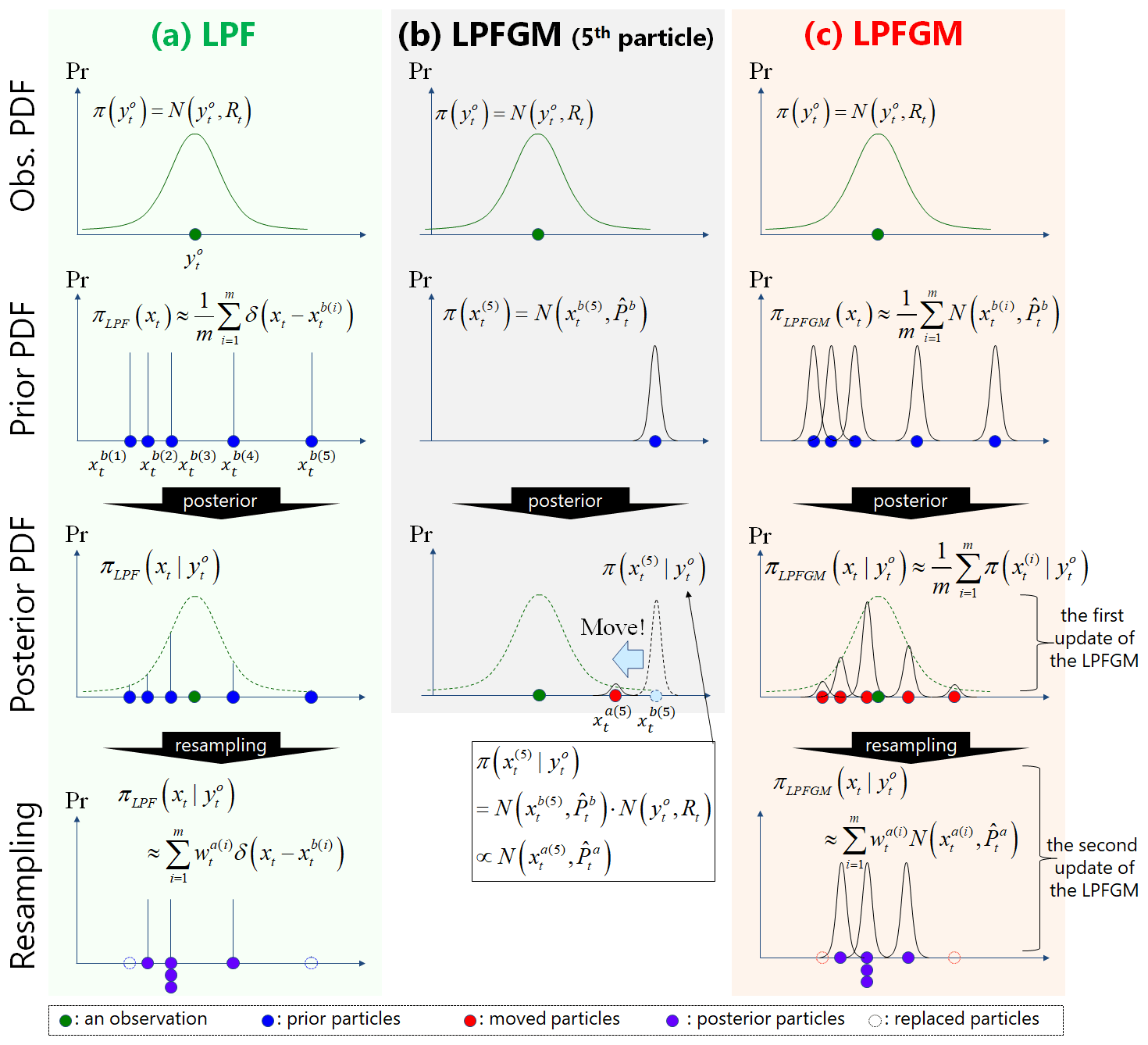
Figure 2A simple scalar example of observation as well as prior and posterior PDFs for (a) LPF, (b) fifth particle of LPFGM, and (c) LPFGM. Green, blue, red, purple, and dashed circles represent an observation and prior particles, moved particles, posterior particles, and replaced particles, respectively.
The two-step update of the LPFGM may appear to use the same observations twice, but this is not true. To understand the principles here, we consider a simple scalar example with H=1.0, with illustrations in Fig. 2. Let be an observation PDF (Fig. 2, top row), and the prior and posterior PDFs of the LPF are given by and ,respectively (Fig. 2a, second and third rows). The LPF employs resampling by approximating the posterior PDF as a combination of prior particles, such that (Fig. 2a, bottom row). Next, we focus on the fifth particle of the LPFGM (Fig. 2b). Prior and posterior PDFs of the fifth particle are given by and , respectively (Fig. 2b, second and third rows). Since the Gaussian kernels are assumed for the prior particles, the center of the posterior kernel moves such that , where and can be computed by the Kalman filter (from the blue circle to the red circle in Fig. 2b). Since the LPFGM moves all particles, the posterior PDF of the LPFGM is given by (Fig. 2c, third row). These movements correspond to the first update of the LPFGM. In contrast to the LPF, the posterior PDF of the LPFGM is approximated by a combination of the posterior Gaussian kernels (red circles of Fig. 2c, third row). The LPFGM employs the resampling based on the moved particles such that (Fig. 2c, bottom row). This resampling corresponds to the second update of the LPFGM. As seen in this example, the two-step update of the LPFGM does not use the same observations twice.
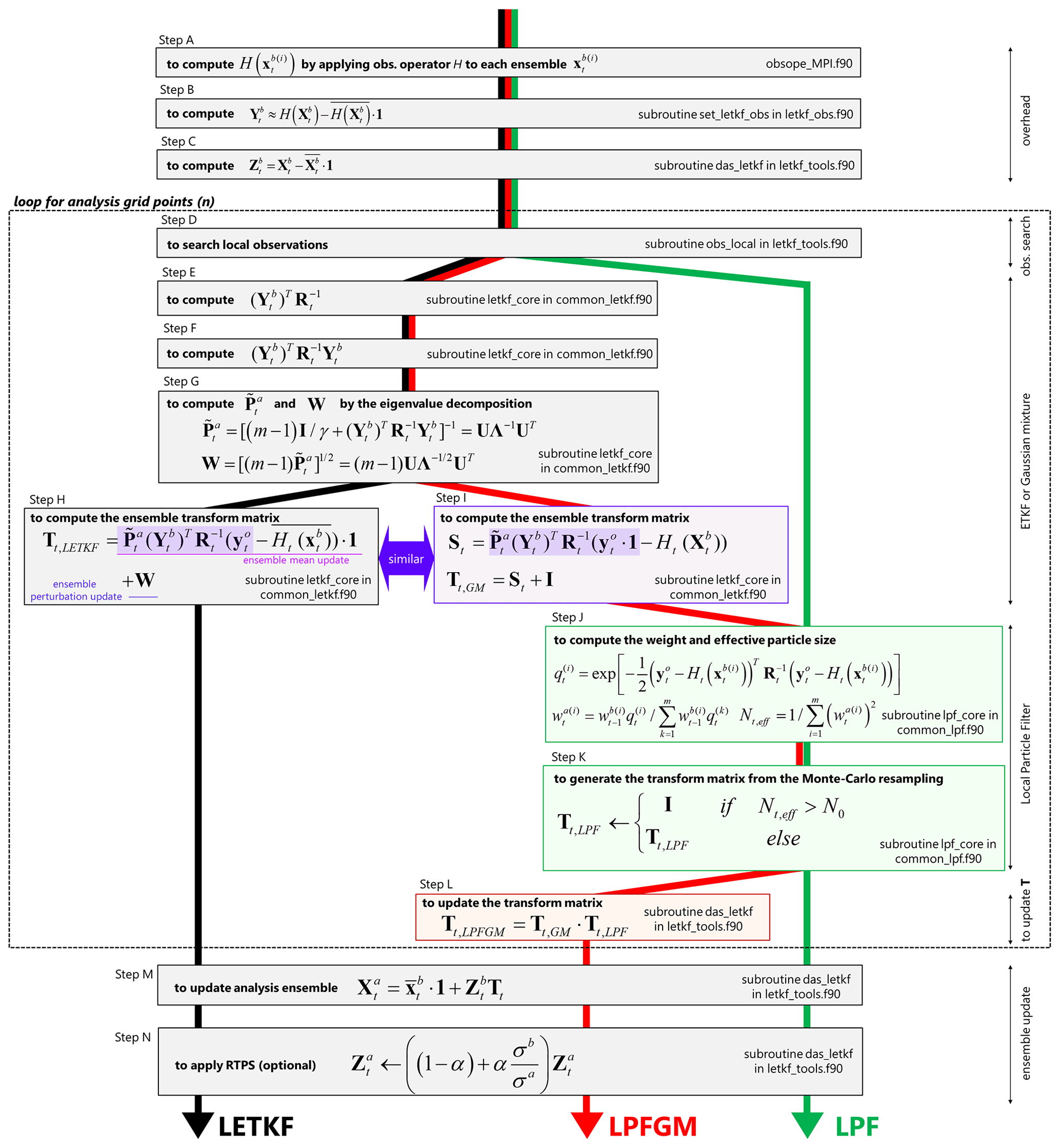
Figure 3Workflows of LETKF, LPFGM, and LPF. Gray, purple, green, and red boxes represent the components of LETKF, a similar component as in the LETKF, the components of the LPF, and a unique component of the LPFGM, respectively. Subroutines and source files are also described in boxes.
2.4 Implementation and computational complexity
We implemented the LPFGM based on the available LETKF code from Miyoshi (2005) and from follow-on studies (Miyoshi and Yamane, 2007; Kondo and Miyoshi, 2019; Kotsuki et al., 2020; https://github.com/takemasa-miyoshi/letkf, last access: 16 November 2022). Figure 3 compares the workflows of the LETKF, LPF, and LPFGM. All DA methods execute the same first four steps (steps A–D). After step D, the LETKF involves four additional steps (steps E–H) to compute TLETKF. The LPF computes the weights of particles (step J), followed by the generation of the transform matrix TLPF (step K). The LPFGM first executes steps E–G, as in the LETKF, and then executes step I to compute TGM, followed by the LPF algorithms to compute TLPF (steps J and K). Finally, the LPFGM multiplies TGM and TLPF to compute TLPFGM (step L). At the end of the process, the transform matrix is applied to the prior perturbation matrix Zb to produce the analysis ensemble (step M) followed by the RTPS (step N).
If the LETKF code is available, the LPF in the transform matrix form can be developed by coding two steps, J and K. The LPFGM can also be developed easily by coding two more steps, I and L, if the LETKF and LPF codes are available.
Table 1Computational complexities of LETKF, LPF, and LPFGM. Each step corresponds to the steps in Fig. 3. Cross marks represent the steps used for LETKF, LPF, and LPFGM.

![]() 1: This computation depends on the localization scale
1: This computation depends on the localization scale![]() 2: These computations assume the diagonal R (i.e., uncorrelated
observation error)
2: These computations assume the diagonal R (i.e., uncorrelated
observation error)
n: system size
m: ensemble size
p: the number of observations
pL: the number of local observations
NMC: the number of times for generating resampling matrices by
Algorithm 1
Here, we compare the computational complexities of the LETKF, LPF, and LPFGM algorithms (Table 1). The total cost (CT) of a DA cycle is identical to the overhead of the assimilation system (CH) plus n times the average local analysis cost (CL) and m times the cost of a one-member model forecast (CM):
where pL is the number of local observations within the localization cut-off radius. We assume that the overhead and model costs are equivalent among the three methods. In addition, the total computational cost of DA usually depends on the local analysis cost (CL):
where NMC is the number of times the resampling matrices are generated by Algorithm 1. The number of local observations pL is usually much greater than the ensemble size m and NMC. In this case, O(m2pL) is dominant for the LETKF and the LPFGM.
Here, the computational cost of LPF is more expensive than that with a simpler resampling algorithm, such as the stochastic uniform resampling (O(m); Penny and Miyoshi 2016; Farchi and Bocquet, 2018), due to the relatively complex Algorithm 1 (O(m2NMC)). We could not use such simpler approaches in this study, since they do not yield ideal resampling matrices that satisfy the two conditions (Eq. 19 and spatially smooth transition of Tt,LPF). The computational cost O(m2NMC) of LPF is still much smaller than the LETKF if NMC≪pL.
3.1 SPEEDY model
This study used the intermediate global atmospheric general circulation model SPEEDY (Molteni, 2003) to compare the LETKF, LPF, and LPFGM. The SPEEDY model is a computationally inexpensive hydrostatic model with fundamental physical parameterization schemes such as surface flux, radiation, convection, cloud, and condensation. The SPEEDY model has 96×48 grid points in the horizontal plane (T30 ∼3.75∘ × 3.75∘) and seven sigma-coordinate seven vertical layers. The SPEEDY model consists of five prognostic variables: temperature (T), specific humidity (Q), zonal wind (U), meridional wind (V) at seven layers, and surface pressure (Ps). The SPEEDY model coupled with the LETKF (SPEEDY-LETKF) has been widely used in DA studies (Miyoshi, 2005, and many follow-on studies, e.g., Miyoshi, 2011; Kondo et al., 2013; Kondo and Miyoshi, 2016, 2019; Kotsuki and Bishop, 2022). We implemented the LPF and LPFGM based on the existing SPEEDY−LETKF code, following the procedures described in Sect. 2.4.
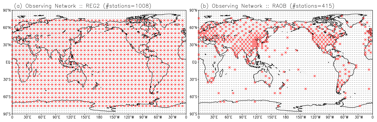
Figure 4Observing networks for (a) REG2 and (c) RAOB experiments. Small black dots and red crosses represent model grid points and observing points, respectively.
3.2 Experimental design
The experimental settings follow the previous SPEEDY−LETKF experiments (Miyoshi, 2005, and follow-on studies, e.g., Kotsuki et al., 2020). A series of idealized and identical experiments (also known as observing system simulation experiments) were conducted without model errors. We first performed a spin-up run for one year, initialized by the standard atmosphere during rest, followed by the nature run started at 00:00 UTC on 1 January of the second year. We assumed diagonal observation error covariance R (i.e., uncorrelated observation error). Gaussian noise was added to the nature run to produce observation data at 6 h intervals. The standard deviations of the Gaussian noise are 1.0 K for T, 1.0 m s−1 for U and V, 0.1 g kg−1 for Q, and 1 hPa for surface pressure. This study considered two observing networks (Fig. 4a and b): the regularly distributed network (hereafter REG2) and the radiosonde-like inhomogeneous network (hereafter RAOB). We observe T, U, and V at all seven layers, whereas Q was observed at the first–fourth layers. The ensemble size is 40, and their initial conditions were taken from an independent single deterministic SPEEDY forecast with sufficient spin-up simulation.
Table 2List of experiments.
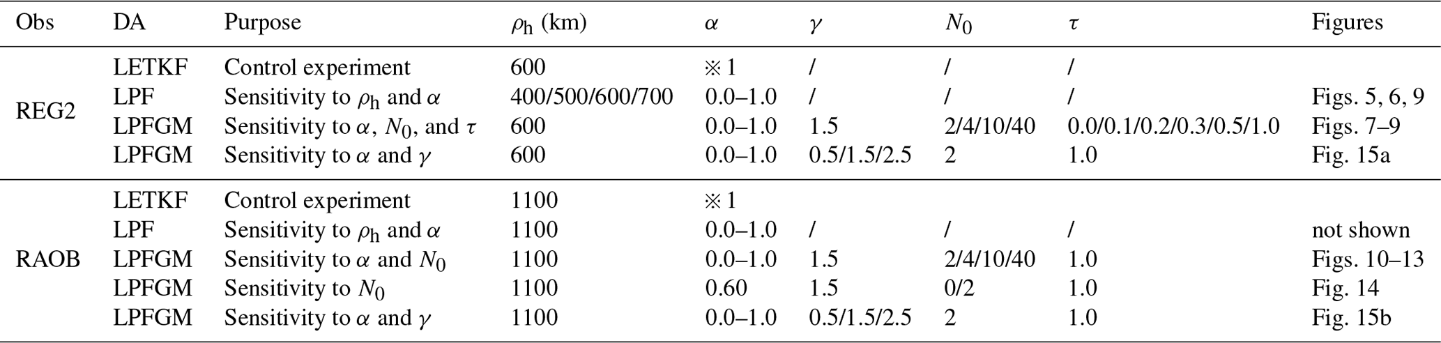
ρh: horizontal localization scale (Eq. 38)
α: relaxation parameter of RTPS (Eq. 8)
γ: amplitude of Gaussian kernel of the LPFGM (Eq. 25)
N0: parameter controls resampling frequency (Eq. 22)
τ: forgetting factor of weight (Eq. 23)![]() 1: Instead of RTPS, the LETKF uses Miyoshi (2011)'s adaptive multiplicative
inflation.
1: Instead of RTPS, the LETKF uses Miyoshi (2011)'s adaptive multiplicative
inflation.
Table 2 summarizes the settings of the LETKF, LPF, and LPFGM experiments. The observation error variance was inflated for the localization by using the Gaussian-based function given by
where l is the localization function, and its inverse l−1 is multiplied and used to inflate R. dh and dv are horizontal and vertical distances (km and log(Pa)) between the observation and analysis grid point. ρh and ρv are tunable horizontal and vertical localization scales (km and log(Pa)). Subscripts “h” and “v” represent horizontal and vertical respectively. This study set the vertical localization scale ρv to be 0.1 log(Pa) following Greybush et al. (2011) and Kondo et al. (2013). The horizontal localization scales of the LETKF were tuned manually before the experiments to minimize the first-guess root mean square error (RMSE) of the fourth layer (∼500 hPa) temperature of the SPEEDY-LETKF, since this is among the most important variables for medium-range NWP.
The LETKF experiments used the adaptive multiplicative inflation method of Miyoshi (2011), in which the inflation factor β was estimated adaptively. On the basis of sensitivity experiments for γ, we chose γ=1.5. Sensitivity to γ is discussed in Sect. 4.3.3.
We first performed a one-year (from January to December) SPEEDY-LETKF experiment over the second year following the one-year spin up. We then performed LETKF, LPF, and LPFGM experiments from January to April in the third year, initialized by the first-guess ensemble of the LETKF at 00:00 UTC on 1 January of the third year. The results from the last three months, i.e., February to April, were used for verification. We assessed the 6 h forecast or background RMSE for T at the fourth model level (∼500 hPa). While this study mainly discusses the RMSE and ensemble spread for T, similar results are observed for other variables. Here, this study will concentrate on the fourth-level T as an important variable for NWPs, since the major goal of this study is to investigate the stabilities of LPF and LPFGM compared with the LETKF. Humidity verification or accounting for nonlinear observation operators and non-Gaussian observation errors are still crucial studies to investigate the advantages of the LPF and LPFGM with respect to the LETKF.
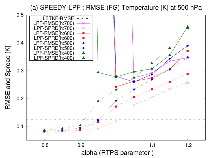
Figure 5Time-mean background RMSEs (solid lines) and ensemble spreads (dashed lines) for T (K) at the fourth model level (∼500 hPa) as a function of RTPS parameter α averaged over three months of the third year (February–April), with REG2 observations. Magenta, red, blue, and green lines are LPF experiments with horizontal localization scales of 700, 600, 500, and 400 km, respectively. Dashed lines represent RMSE of LETKF (0.1257 K), with adaptive multiplicative inflation instead of RTPS.
4.1 Experiments with a regularly distributed observing network
We first compare the LETKF, LPF, and LPFGM with REG2, where the manually tuned horizontal localization scale for the LETKF is 600 km. First, sensitivities to the horizontal localization scale (ρh) and RTPS parameter (α) are investigated for the LPF. Figure 5 indicates the time-mean background RMSEs and ensemble spreads for LETKF and LPF. The LPF requires large inflation (α≥1.0) to avoid filter divergence. With large inflation (α≥1.0), the LPF experiment with ρh=600 km resulted in the smallest RMSEs among the three LPF experiments. The best-performing localization scale of LPF was found to be similar to that of the LETKF. The four LPF experiments exhibited larger RMSEs than the LETKF, as demonstrated by the previous studies with a low-dimensional L96 model (Poterjoy, 2016; Penny and Miyoshi, 2016; Farichi and Bouquet, 2018). The LPF experiment with ρh=700 km shows filter divergence when α=1.0. The ensemble spreads of LPF are smaller than the RMSEs when α=1.0. This under-dispersive ensemble is a typical behavior of LPF (e.g., Poterjoy and Anderson, 2016).
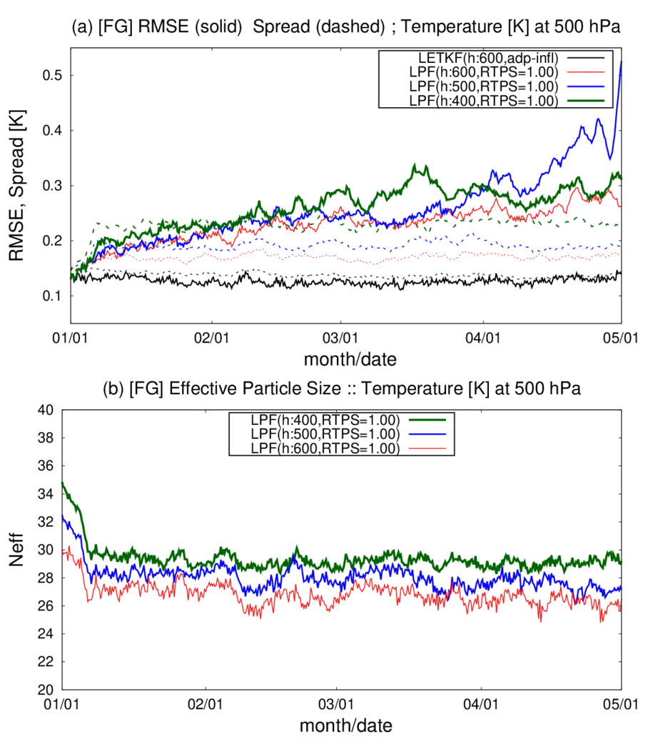
Figure 6Time series of globally averaged background (a) RMSEs (solid lines) and ensemble spreads (dashed lines) for T (K) and (b) effective particle size Neff at the fourth model level (∼500 hPa), with REG2 observations. Black lines show the LETKF. Red, blue, and green lines are the LPF experiments, with localization scales of 600, 500, and 400 km, respectively. RTPS parameter α is set to 1.00 in all three LPF experiments. The abscissa shows month and day.
Second, we compare the time series of the background RMSEs, ensemble spreads, and effective particle sizes Neff (Fig. 6). The RMSE and ensemble spread are consistent in the LETKF. However, the LPF generally shows smaller ensemble spreads than the RMSEs. Since the beginning of the experiments on 1 January, the three LPF experiments showed rapid increases in the ensemble spread (Fig. 6a) and a rapid decrease in the effective particle size (Fig. 6b) within two weeks. After the rapid changes, the ensemble spreads and effective particle sizes were stabilized. The three LPF experiments increased RMSEs until the beginning of March. The LPF with ρh=500 km showed filter divergence in April. The LPF with ρh=400 km and ρh=600 km also showed increasing trends in RMSE until the end of April, while their ensemble spreads and effective particle sizes were stable.
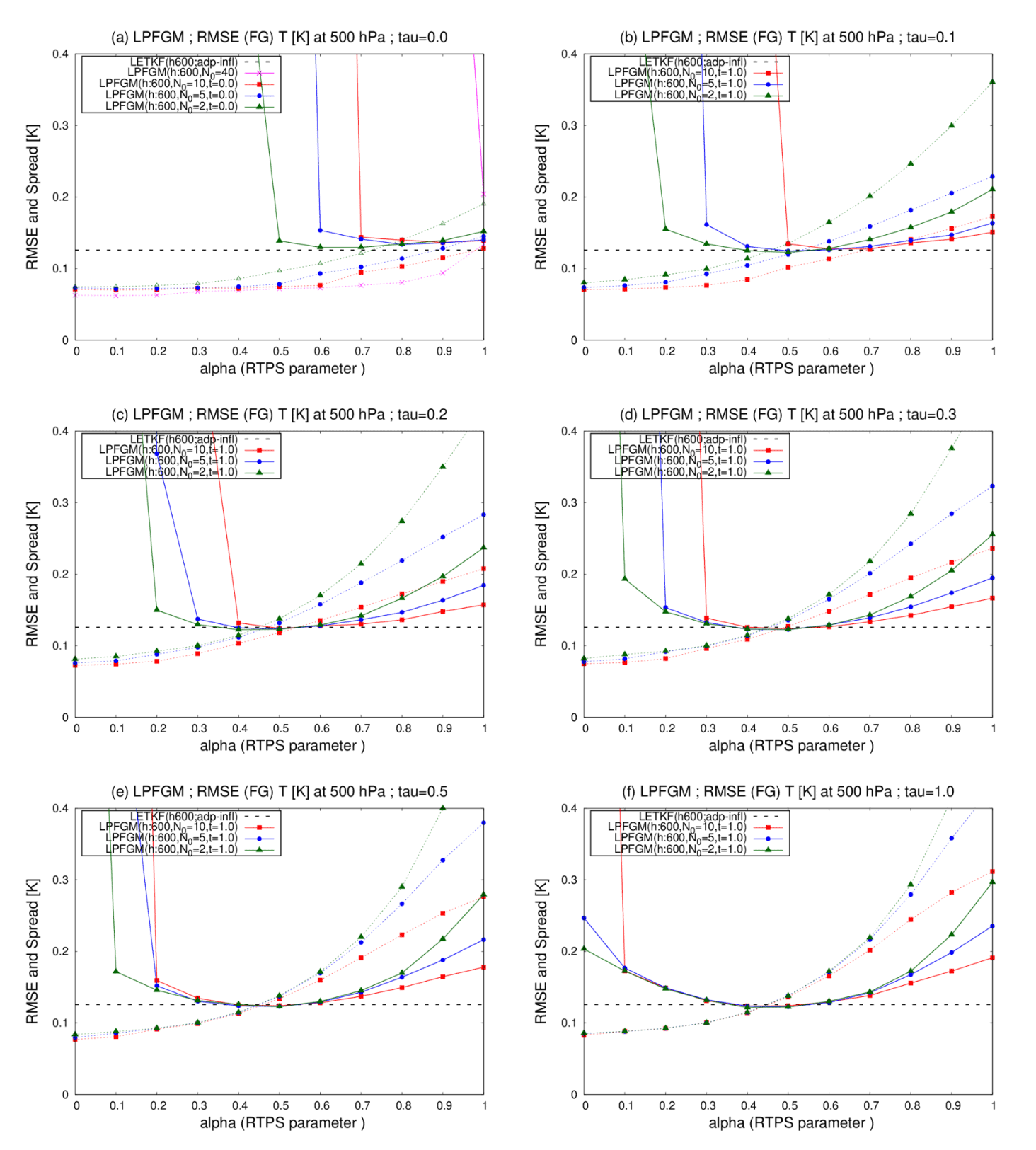
Figure 7Similar to Fig. 5 but for the LPFGM with REG2 and 600 km localization scale. Magenta, red, blue, and green lines show the cases with N0=40, 10, 5, and 2, respectively. Dashed lines represent RMSE of LETKF (0.1257 K). Panels show the LPFGM with forgetting factors for (a) τ=0.0, (b) τ=0.1, (c) τ=0.2, (d) τ=0.3, (e) τ=0.5, and (f) τ=1.0, respectively.
Next, sensitivities to the RTPS parameter (α), resampling frequency (N0), and forgetting factor (τ) are investigated for the LPFGM. The best performing localization scale of LPF was identical to that of the LETKF (Fig. 5). Therefore, we choose the same 600 km localization scale for the LPFGM. Figure 7 compares the time-mean background RMSEs and ensemble spreads for LETKF and LPFGM. In the LPFGM experiments, we investigate six experimental settings for τ=0.0, 0.1, 0.2, 0.3, 0.5, and 1.0. With τ=0.0 (Fig. 7a), the LPFGM shows RMSEs similar to those of LETKF, with best-performing parameters for α and N0. Regulating the resampling frequency (N0) would be needed for LPFGM, because the LPFGM shows filter divergence when resampling is employed at all assimilation steps, excluding the case of α=1.0 (magenta line in Fig. 7a). The LPFGM employs two ensemble updates: the Gaussian mixture and resampling. Owing to the first update by the Gaussian mixture, the LPFGM would not require resampling at all assimilation steps. With τ=0.0, the best-performing relaxation parameter α is approximately 0.6–0.9, excluding the case employing resampling at all assimilation steps.
Increasing τ leads to the LPFGM being less sensitive to the resampling parameter N0 and RTPS parameter α (Fig. 7b–f), implying that the LPFGM is more stable when the LPFGM forgets weights (τ≥0.1). Additionally, the LPFGM requires less inflation (i.e., smaller α) when the forgetting factor τ becomes larger. Owing to the first update by the Gaussian mixture, succeeding weights completely may be unnecessary for the LPFGM. In addition, the method of succeeding weights in the local PF is not trivial, because the weights would move with the dynamical flow. Because the results of the LPFGM experiments without weight succession (τ=1.0) were superior to those with weight succession (τ=0.0), the remainder of this paper focuses on the LPFGM experiments without weight succession (τ=0.0).
.
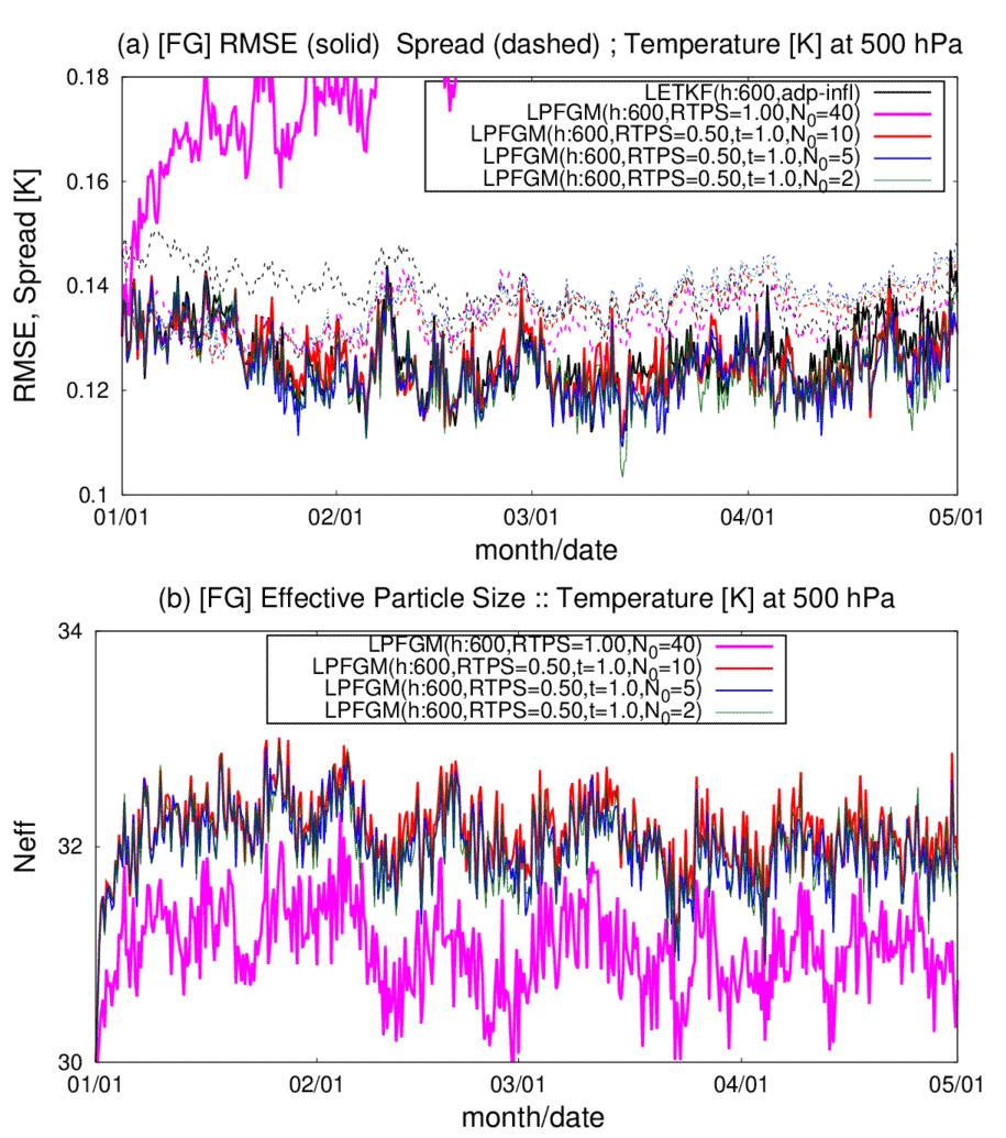
Figure 8Similar to Fig. 6, but showing the LPFGM experiments with REG2 and 600 km localization scale. Magenta, red, blue, and green lines are LPFGM experiments with N0=40, 10, 5, and 2, respectively. Forgetting factor τ is 1.0. The RTPS parameter is set to 1.00 in the experiment with N0=40 (i.e., all-time resampling) and to 0.50 for in other experiments.
The time series of background RMSEs and the effective particle sizes for LPFGM experiments show that the LPFGM with every-time resampling (N0=40) exhibits large RMSEs and the smallest effective particle sizes (Fig. 8, magenta). In contrast, the LPFGM experiments with infrequent resampling (N0=10, 5, and 2) show small RMSEs similar to that of the LETKF and maintain larger effective particle sizes than the LPF (Fig. 8, red, blue, and green lines).
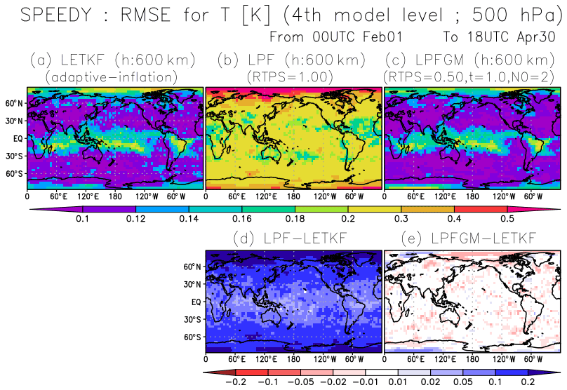
Figure 9Spatial patterns of background RMSE for T (K) at the fourth model level (∼500 hPa) for (a) LETKF, (b) LPF, and (c) LPFGM, with best-performing localization scale and RTPS parameter, averaged over February–April with REG2 and 600 km localization scale. Panels (d) and (e) show the differences between LETKF-LPF and LETKF-LPFGM, respectively. The warm (cold) color indicates that the LPF or LPFGM is better (worse) than the LETKF.
Finally, we compare the spatial patterns of the RMSEs at a fourth model level for the LETKF, LPF, and LPFGM, with best-performing parameter settings (Fig. 9). The LETKF and LPFGM show larger RMSEs in the tropics and polar regions (Fig. 9a and c), possibly because of uncertainties from convective dynamics in the tropics and sparser observations in the polar regions. The LPF shows a larger RMSE than the LETKF globally (Fig. 9b and d). In contrast, slight improvements were observed globally in the LPFGM relative to the LETKF, as indicated by generally warm colors in Fig. 9e, especially around the North Pole.
4.2 Experiments with a realistic observing network
Here, we compare the LETKF, LPF, and LPFGM with the realistic observing network RAOB. With this spatially inhomogeneous observing network, all LPF experiments showed filter divergence, even with a broad range of the localization and RTPS parameters. Since there are fewer assimilated observations in RAOB than in REG2, the weight collapse would not be the primary cause of the LPF filter divergence. Because the LPF creates posterior particles by linearly combining prior particles, it is preferable for the LPF to have observations within the range of the prior particles. Filter divergence must be prevented by maintaining synchronization between the LPF and the observations. The LPF would require more observations for the synchronization than the LETKF, which was also shown in the authors' initial tests with L96. In addition, the LPFGM was unstable with weight succession (τ=0.0). Therefore, this section focuses on the comparison of the LETKF and LPFGM without weight succession (τ=1.0) only.
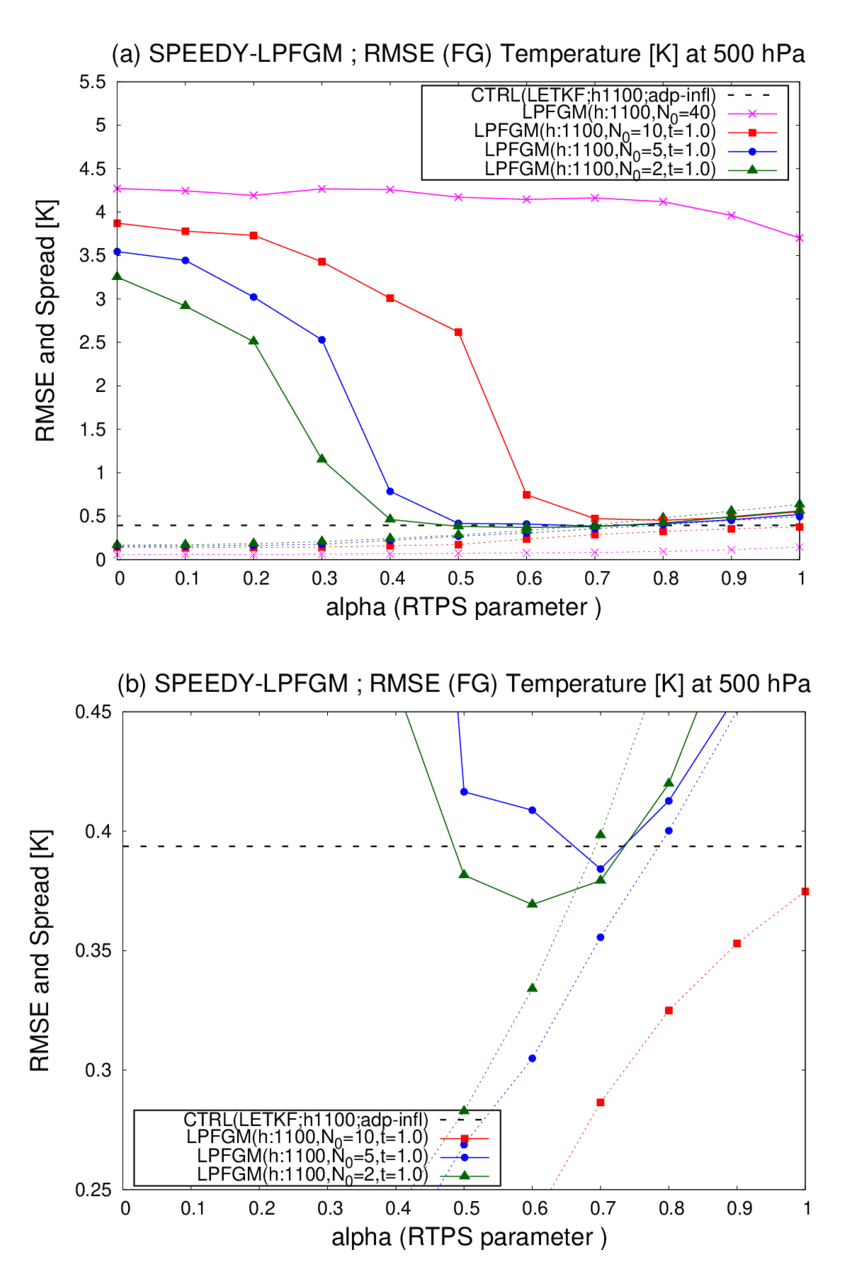
Figure 10Similar to Fig. 5 but showing the LPFGM experiments with the RAOB and 1100 km localization scale. Magenta, red, blue, and green lines are the LPFGM experiments with N0=40, 10, 5, and 2, respectively. Forgetting factor τ is fixed at 1.0. Dashed black lines represent the RMSE of the LETKF (0.4762 K); (b) enlarges (a) for the range of the RMSE of 0.25–0.45.
First, sensitivities to the RTPS parameter (α) and resampling frequency (N0) are investigated for the LPFGM. Figure 10 compares the time-mean background RMSEs and ensemble spreads for the LETKF and LPFGM. The best-performing horizontal localization scale for the LETKF is 1100 km, and the same localization scale is used for the LPFGM. The LPFGM with every-time resampling (N0=40) shows the largest RMSEs (Fig. 10a, magenta). By contrast, some LPFGM experiments show smaller RMSEs than the LETKF (Fig. 10b). In this experimental setting, the resampling parameter of N0=2.0 shows the most stable performance. With N0=2.0, the LPFGM outperforms the LETKF slightly for α=0.5–0.7 (green line of Fig. 10b).
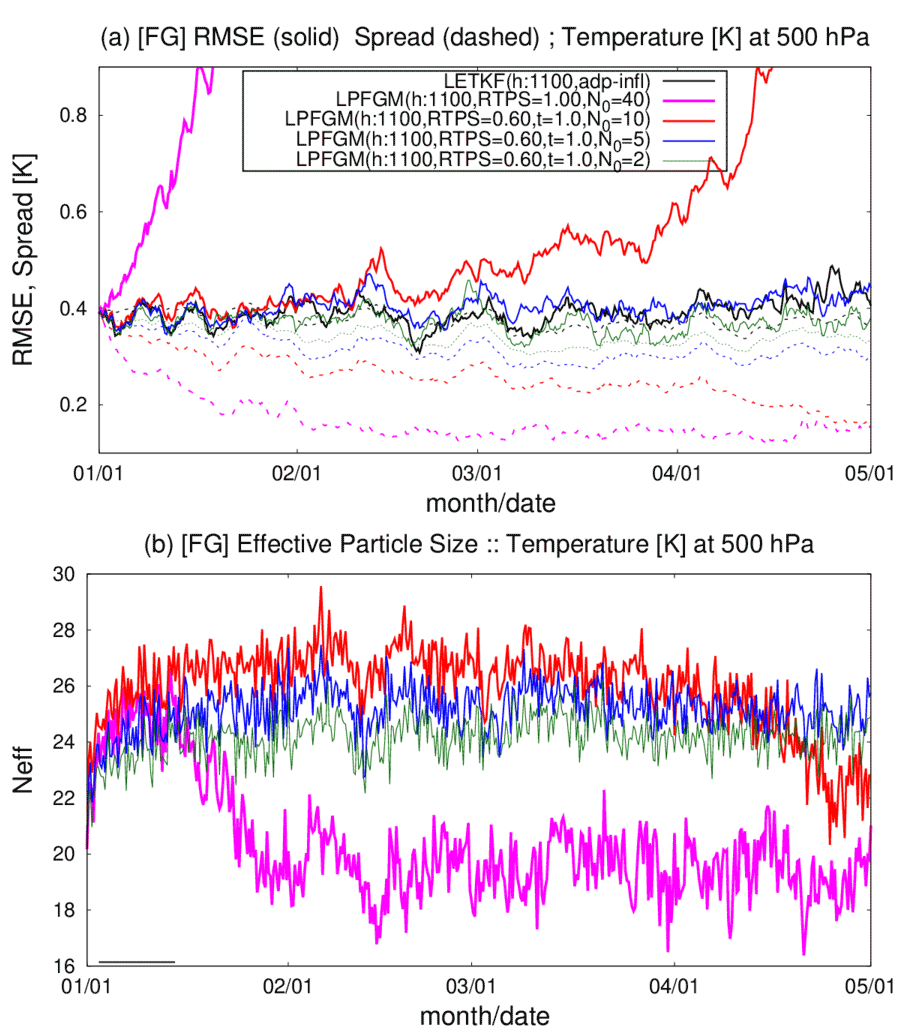
Figure 11Similar to Fig. 8 but showing the LPFGM experiments with the RAOB and 1100 km localization scale. Magenta, red, blue, and green lines are LPFGM experiments with N0=40, 10, 5, and 2, respectively. Forgetting factor τ is 1.0. The RTPS parameter is set to 1.00 in the experiment with N0=40 (i.e., all-time resampling) and to 0.60 for in other experiments.
The time series of the background RMSEs and effective particle sizes show that the LPFGM with every-time resampling (N0=40; Fig. 11a, magenta) and relatively frequent resampling (N0=10; Fig. 11a, red) caused filter divergences. The times when the filters diverged seem to correspond to the times when the effective particle sizes decreased (Fig. 11b, magenta and red). This reduction in effective particle size is a typical sign of filter divergence for PF (Snyder et al., 2008). One may speculate that the assumption of in the LPFGM (Sect. 2.3) would be a reason for the filter divergence. However, adopting the appropriate norm () for the LPFGM did not eliminate the filter divergence (not shown). An effective solution for avoiding the filter divergence with every-time resampling is still unknown, but a possible reason is the method of creating a transform matrix using the Monte Carlo method that approximates two ideal conditions (Eq. 19 and a spatially smooth transition). For deeper understanding, using other resampling techniques such as the optimal transport (see Sect. 4.3.2) would be useful. In contrast, the LPFGM experiments with infrequent resampling (N0=5 and 2) show stable RMSEs and maintain a larger effective particle size. These stable LPFGM experiments maintain the amplitude of the ensemble spreads similarly to that of the RMSEs.
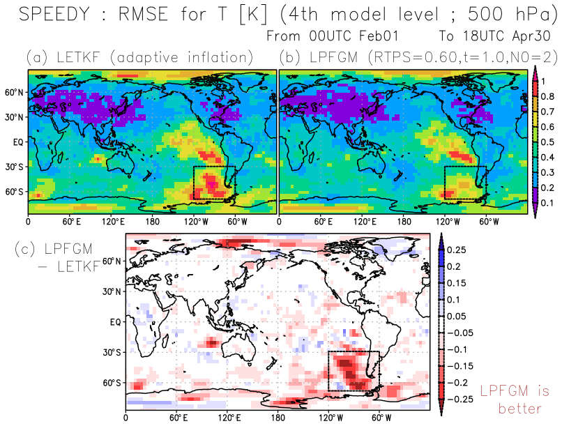
Figure 12Spatial patterns of background RMSE for T (K) at the fourth model level (∼500 hPa) for (a) LETKF and (b) LPFGM, averaged over February–April, with RAOB and 1100 km localization scale. Panel (c) shows the difference between LETKF and LPFGM. Warm (cold) color indicates that the LPFGM is better (worse) than the LETKF. Black dashed rectangles show the region (120–60∘ W and 70–30∘ S) where the differences between LETKF and LPFGM are investigated in Fig. 14.
We further explore regions where the LPFGM outperforms the LETKF. Figure 12 compares the space-based patterns of the background RMSEs for T (K) at the fourth model level for LETKF and LPFGM. Errors in sparsely recognized regions – such as the South Pacific Ocean, Indian Ocean, and polar regions – tend to be larger (Fig. 12a and b). The LPFGM outperforms the LETKF in such sparsely observed regions (Fig. 12c). The regions showing improvements correspond to the regions where the ensemble spreads and first-guess non-Gaussianity are larger (Fig. 13). Here, we measure the non-Gaussianity by means of Kullback–Leibler divergence (Kullback and Leibler, 1951).
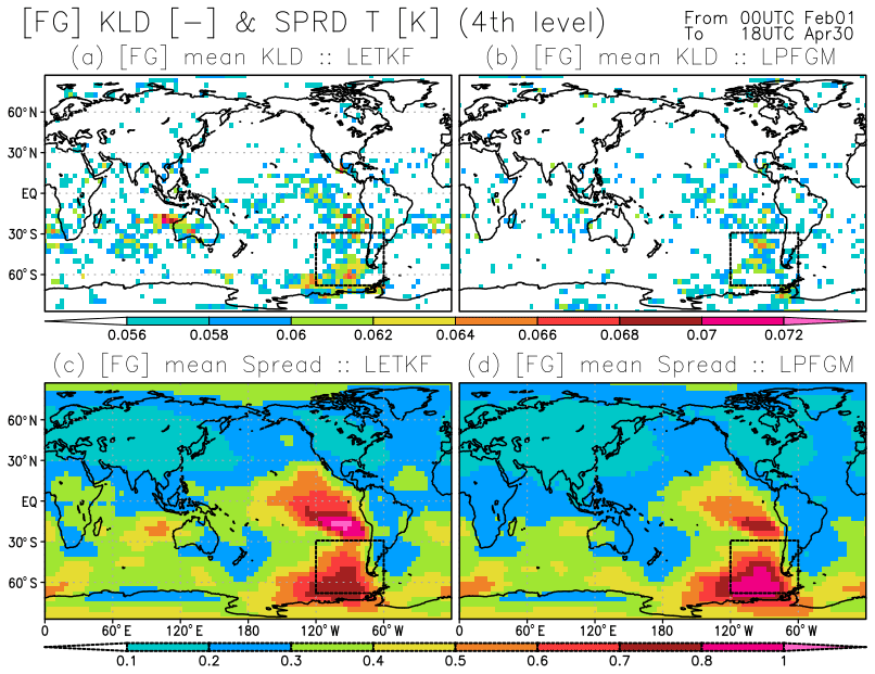
Figure 13Spatial distributions of the background (a, b) Kullback–Leibler divergence and (c, d) ensemble spread for T (K) at the fourth model level (∼500 hPa), averaged over February–April, with RAOB and 1100 km localization scale; (a, c) and (b, d) show the LETKF and LPFGM, respectively. Black dashed rectangles show the region (120–60∘ W and 70–30∘ S) where the differences between LETKF and LPFGM are investigated in Fig. 14.
The first update of the LPFGM (the Gaussian mixture) is similar to the LETKF update, as discussed. Therefore, the improvements of the LPFGM with respect to the LETKF would be owing to the resampling step. Previous studies demonstrated that the LPF outperformed the LETKF for non-Gaussian DA with non-Gaussian observation and prior PDFs (Poterjoy and Anderson, 2016; Poterjoy, 2016; Penny and Miyoshi, 2016). Therefore, the improvements of the LPFGM would come from the consideration of non-Gaussian prior PDF in sparsely observed regions.
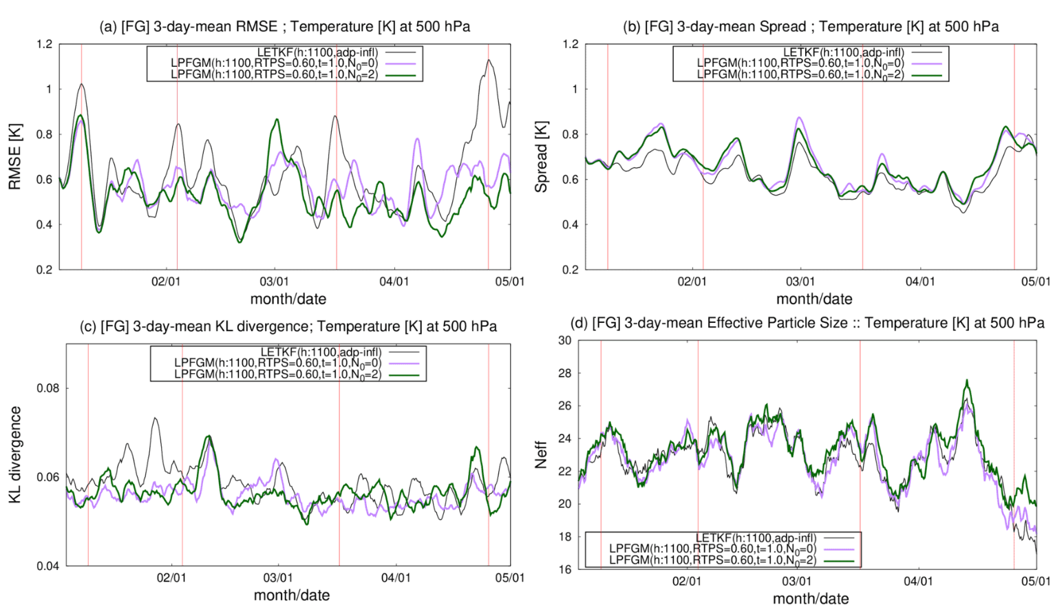
Figure 14Time series of 3 d-mean (a) RMSE (K), (b) ensemble spread (K), (c) Kullback–Leibler divergence, and (d) effective particle size Neff at fourth model level temperature T, averaged over the region indicated by rectangles in Figs. 12 and 13 (120–60∘ W and 70–30∘ S). The black line represents the LETKF. Green and purple lines are the LPFGM whose resampling frequencies N0 are 2 and 0, respectively. Vertical red lines represent the cases when the LETKF shows large RMSE greater than 0.8 K. In (d), the effective particle size is also computed for the LETKF using the first-guess ensemble.
Finally, we investigate the region where the difference in RMSE between the LETKF and LPFGM is large (120–60∘ W and 70–30∘ S; indicated by black dashed rectangles in Figs. 12 and 13). Figure 14 compares the time series of RMSE, ensemble spread, effective particle size, and Kullback–Leibler divergence averaged over the region for the LETKF and LPFGM. Here, we conducted an additional LPFGM experiment that employs no resampling (i.e., N0=0) to investigate the importance of resampling. Vertical red lines in Fig. 14 represent the cases when the LETKF has large RMSEs greater than 0.8 K. Figure 14a indicates that the LPFGM tends to mitigate large RMSEs, which is in contrast to the LETKF. Since no significant increase is seen in the Kullback–Leibler divergence at the four cases (Fig. 14c), the large RMSEs of LETKF would not be caused by analyses with highly non-Gaussian first-guess ensembles. For the last three cases, the LPFGM has significantly smaller RMSEs than the LETKF. The improvement of the LPFGM would be partially led by larger ensemble spread than the LETKF (Fig. 14b). However, the LPFGM with resampling (N0=2) outperforms the LPFGM without resampling (N0=0), indicating that resampling improves the RMSE. The LETKF and LPFGM exhibit reduced effective particle size at the three later cases (Fig. 14d). Because of the smaller effective particle size, fewer ensembles predict states that are closer to observations, and the LPFGM employed more resampling in the region. In addition to the particle shift, the LPFGM would reduce RMSE further by the resampling.
The LPFGM occasionally resulted in larger RMSE than the LETKF (e.g., beginning of March in Fig. 14a). However, the LPFGM has the potential to outperform the LETKF overall by reducing the RMSE in sparsely observed regions. While operational NWP systems assimilate massive observations, the LPFGM would be useful when spatially and temporally sparse observations are used – e.g., in the twentieth-century reanalysis projects (e.g., Compo et al., 2011; Laloyaux et al., 2018) and paleoclimate reconstructions (Acevedo et al., 2017; Okazaki and Yoshimura, 2017).
4.3 Factors requiring further investigation
Finally, we discuss other issues for potential further improvement of the LPF and LPFGM in future studies.
4.3.1 Inflation
This study used the RTPS to inflate the posterior perturbation for the LPF and LPFGM. As shown in Figs. 5, 7, and 10, the RMSEs of the LPF and LPFGM are sensitive to the RTPS parameter. There is a need to investigate methods that estimate the RTPS parameter adaptively, as in the EnKF (Ying and Zhang, 2015; Kotsuki et al., 2017b). However, the adaptive relaxation methods used in the EnKF cannot be applied directly to the LPF, because they use the innovation statistics (Desroziers et al., 2005) that assume analysis updates by the Kalman gain. Therefore, substantially different adaptive relaxation methods should be investigated for the LPF and LPFGM.
An alternative method of inflation is adding random noise to the transform matrix (Potthast et al., 2019). Regulating the amplitude of the random noise was not trivial in the authors' preliminary experiments with L96 (not shown). Random noise that is too small results in a loss of diversity of posterior particles, whereas excessively large random noise results in an overly dispersive ensemble. Potthast et al. (2019) also suggested estimating the amplitudes of the random noise based on the innovation statistics. However, determining the minimum and maximum values of the amplitudes was not trivial from the authors' experience with L96. Therefore, a method to determine the optimum amplitude of random noise should be investigated as well. Moreover, additive inflation methods, as used in the EnKF, can be beneficial for producing diverse prior particles (Mitchell and Houtekamer, 2000; Corazza et al., 2003). For example, Penny and Miyoshi's (2016) LPF applied an additive inflation Gaussian noise whose variance is scaled to a magnitude of local analysis error variance. Investigating better and adaptive inflation methods is very important to stabilize LPFs.
4.3.2 Transform matrix for LPF
The transform matrix significantly affects the filter performance. Farchi and Bocquet (2018) demonstrated that the optimal transport method of Reich (2013) resulted in lower RMSE than the commonly used stochastic uniform resampling approach with the L96 model. However, it is not clear if optimal transport is beneficial for high-dimensional systems such as the SPEEDY model.
In this study, all-time resampling was detrimental for the LPFGM experiments (Figs. 7 and 10).This may be due to the MC resampling that does not exactly but only approximately satisfies Eq. (19) (). With a small effective particle size, the MC resampling almost satisfies Eq. (19), since the resampling is not affected by the sampling noise in the selection of particles. In contrast, satisfying Eq. (19) is more difficult when the effective particle size is larger due to the sampling noise. A possible solution to this problem is to use the optimal transport method (Reich, 2013) that satisfies Eq. (19) exactly. Another essential property for local PFs is the spatially smooth transition of the transform matrix. The optimal transport method would also be useful for ensuring the spatially smooth transition of the transform matrix, because the posterior weights in nearby grids are typically similar. It is necessary to investigate better methods for generating resampling matrices.
4.3.3 Tunable parameters of LPF and LPFGM
The tunable parameters of the LPF and LPFGM should be investigated further. For example, parameter N0, which controls the resampling frequency, significantly affected the filter accuracy and stability. Adaptive determination of this parameter can prevent time-consuming parameter tuning.

Figure 15Time-mean background RMSEs for T (K) at the fourth model level (∼500 hPa) as a function of RTPS parameter α, averaged over three months of the third year (February–April); (a) shows REG2 with 600 km localization scale, and (b) shows RAOB with 1100 km localization scale. Red, blue, and green lines are LPFGM experiments where γ=2.5, 1.5, and 0.5, respectively. Black dashed lines represent RMSE of LETKF (0.1257 K) with adaptive multiplicative inflation instead of RTPS. Other parameters are set to be the best-performing parameters: N0=2 and τ=1.0.
The sensitivity to parameter γ should also be investigated for the LPFGM. WP22 proposed using γ=2.5. Since γ controls the amplitude and width of Gaussian kernels, the filter accuracy and stability of the LPFGM would be sensitive to this parameter. We briefly examined the sensitivity to this parameter with REG2 and RAOB (Fig. 15; γ=2.5, 1.5, and 0.5 for red, blue, and green lines). The results indicate that the filter accuracy of the LPFGM is sensitive to this parameter, especially for a spatially inhomogeneous RAOB observing network. For our experimental settings, the best-performing γ was 1.5 for both REG2 and RAOB. However, the optimal parameter would differ for different models, observing networks, and observing frequency. Also, there might be a relation between the optimal γ and ensemble size. Therefore, adaptive determination of this parameter is helpful.
The LPFGM without weight succession (τ=1.0) resulted in lower RMSE than that with weight succession (τ=0.0). However, the optimal parameter τ would be somewhere between 0.0 and 1.0. In addition, the weight succession at each model grid point would be suboptimal. Hence, the method for weight succession should also be explored further.
This study aims to develop a software platform for the LETKF, LPF, and LPFGM with the intermediate global atmospheric model SPEEDY. The main results of this investigation are briefly listed as follows:
-
The LPF and LPFGM were developed with only minor modifications to the existing LETKF system with the SPEEDY model.
-
With dense observations (REG2), the LPF showed stable filter performance with large inflation by the RTPS. The best-performing localization scale of the LPF was identical to that of the LETKF. The LPF forecast was less accurate than the LETKF forecast. With sparse observations (RAOB), the LPF did not work.
-
The LPFGM showed more stability and lower forecast RMSEs than the LPF. In addition to the RTPS parameter, regulating the resampling frequency and the amplitude of Gaussian kernels was important for the LPFGM. The LPFGM without weight succession resulted in more stability and lower RMSEs than that with weight succession. With RAOB, the LPFGM forecast was more accurate than the LETKF forecast in sparsely observed regions, where the background ensemble spread and non-Gaussianity are larger.
As discussed in Sect. 4.3, there is much room for improvement in the LPF and LPFGM. While the LPFGM potentially provides a more accurate forecast than the LETKF, the LPFGM has more tunable parameters than the LETKF. Manually tuning these parameters by trying numerous experiments is computationally expensive. Therefore, adaptive methods for determining such tuneable parameters need to be explored. Also, it is important to investigate computationally more efficient methods to generate resampling matrices for the LPF and LPFGM.
The SPEEDY-based LETKF, LPF, and LPFGM used in this study are available as open-source software on GitHub (https://github.com/skotsuki/speedy-lpf, last access: 16 November 2022). This can act as a useful platform to investigate the LPF and LPFGM further in comparison with the well-known LETKF.
Here, we describe the derivations of Kalman gain and analysis error covariance (Eqs. 5 and 6). The Kalman gain can be changed as follows:
Using , analysis error covariance can be changed as follows:
Consequently, we can derivate from Eq. (A9) and from Eq. (A4).
This appendix investigates the number of required samples for the MC resampling to obtain accurate transform matrices stably. Here, we assume that 10 000 samples are sufficient to obtain an accurate transform matrix (). An absolute error (AE) of the transform matrix with G samples () is defined to measure the accuracy of the transform matrix:
Figure B1 shows the AE as a function of the number of samples for ensemble members 10, 20, 40, and 80. For this investigation, we obtained 1000 independent weights generated by uniform random numbers, and average, minimum, and maximum AEs of 1000 cases are shown. For four ensembles, AEs decrease rapidly for the first 1000 samples, followed by a gradual decrease until AE = 0. To reach 10 % of initial error at NMC=1, MC resampling requires about 70, 300, 400, and 600 samples for ensemble members 10, 20, 40, and 80. It suggests that more ensemble requires more samples to obtain an accurate transform matrix stably by means of MC resampling.

Figure B1Absolute errors of the transform matrix of MC resampling as a function of the number of samples (NMC) verified against the transform matrix with 10 000 samples. Absolute errors are computed for 1000 independent cases that have different weights generated by uniform random numbers. Black bold lines show the average of 1000 cases, and gray shades represent minimum and maximum errors of the 1000 cases. Panels (a)–(d) show experiments with 10, 20, 40, and 80 ensembles, respectively. Dashed line shows the 10 % of initial error at NMC=1.
The developed data assimilation system is available at (https://github.com/skotsuki/speedy-lpf, last access: 16 November 2022), which is based on the existing SPEEDY-LETKF system (https://github.com/takemasa-miyoshi/letkf, last access: 16 November 2022; Miyoshi, 2022). The data assimilation system used in this manuscript is archived on Zenodo (https://doi.org/10.5281/zenodo.6586309; Kotsuki, 2022). Due to the large volume of data (>6 TB) and limited disk space, processed data and scripts for visualization are also shared on Zenodo at the same link.
SK developed the data assimilation system, conducted the experiments, analyzed the results, and wrote this manuscript. TM is the PI and directed the research, with substantial contribution to the development of this paper. KK developed the data assimilation system with SK. RP contributed substantially to the introduction of the LPFGM to the standard local particle filter.
The contact author has declared that none of the authors has any competing interests.
Publisher's note: Copernicus Publications remains neutral with regard to jurisdictional claims in published maps and institutional affiliations.
The authors thank the members of the Data Assimilation Research Team, RIKEN Center for Computational Science (R-CCS), for valuable suggestions and discussions. Shunji Kotsuki thanks Ken Oishi of Chiba University for the useful discussions. The experiments were performed using the Supercomputer for earth Observation, Rockets, and Aeronautics (SORA) at JAXA.
This research has been supported by the Japan Aerospace Exploration Agency (Precipitation Measuring Mission), the Ministry of Education, Culture, Sports, Science and Technology (advancement of meteorological and global environmental predictions utilizing observational “Big Data” of the social and scientific priority issues (Theme 4) to be tackled by using post K computer of the FLAGSHIP2020 Project), the Ministry of Education, Culture, Sports, Science and Technology (the Program for Promoting Researches on the Supercomputer Fugaku (Large Ensemble Atmospheric and Environmental Prediction for Disaster Prevention and Mitigation) of MEXT (grant no. JPMXP1020200305)), the Ministry of Education, Culture, Sports, Science and Technology (the Initiative for Excellent Young Researchers), the Ministry of Education, Culture, Sports, Science and Technology (JST AIP JPMJCR19U2, JST PRESTO MJPR1924, JST SICORP JPMJSC1804, JST CREST JPMJCR20F2, JST SATREPS JPMJSA2109), the Ministry of Education, Culture, Sports, Science and Technology (KAKENHI (grant nos. JP18H01549, JP19H05605, 21H04571, and 21K13995)), COE research grant in computational science from Hyogo Prefecture and Kobe City through Foundation for Computational Science, RIKEN Pioneering Project “Prediction for Science”, and IAAR Research Support Program of Chiba University.
This paper was edited by Yuefei Zeng and reviewed by Steve G. Penny and Javier Amezcua.
Acevedo, W., Fallah, B., Reich, S., and Cubasch, U.: Assimilation of pseudo-tree-ring-width observations into an atmospheric general circulation model, Clim. Past, 13, 545–557, https://doi.org/10.5194/cp-13-545-2017, 2017.
Ades, M. and van Leeuwen, P. J.: An exploration of the equivalent weights particle filter, Q. J. Roy. Meteor. Soc., 139, 820–840, https://doi.org/10.1002/qj.1995, 2013.
Ades, M. and van Leeuwen, P. J.: The equivalent-weights particle filter in a high-dimensional system, Q. J. Roy. Meteor. Soc., 141, 484–503, https://doi.org/10.1002/qj.2370, 2015.
Anderson, J. L.: An Ensemble Adjustment Kalman Filter for Data Assimilation, Mon. Weather Rev., 129, 2884–2903, https://doi.org/10.1175/1520-0493(2001)129<2884:AEAKFF>2.0.CO;2, 2001.
Anderson, J. L. and Anderson, S. L.: A Monte Carlo implementation of the nonlinear filtering problem to produce ensemble assimilations and forecasts, Mon. Weather Rev., 127, 2741–2758, https://doi.org/10.1175/1520-0493(1999)127<2741:AMCIOT>2.0.CO;2, 1999.
Bengtsson, T., Snyder, C., and Nychka, D.: Toward a nonlinear ensemble filter for high-dimensional systems, J. Geophys. Res., 108, D24, https://doi.org/10.1029/2002JD002900, 2003.
Bishop, C., Etherton, B., and Majumdar, S.: Adaptive Sampling with the Ensemble Transform Kalman Filter, Part I: Theoretical Aspects, Mon. Weather Rev., 129, 420–436, https://doi.org/10.1175/1520-0493(2001)129<0420:ASWTET>2.0.CO;2, 2001.
Burgers G., van Leeuwen P. J., and Evensen, G.: Analysis scheme in the ensemble Kalman filter, Mon. Weather Rev., 126, 1719–1724, https://doi.org/10.1175/1520-0493(1998)126<1719:ASITEK>2.0.CO;2, 1998.
Compo, G. P., Whitaker, J. S., Sardeshmukh, P. D., Matsui, N. R., Allan, J., Yin, X., Gleason, B. E., Vose, R. S., Rutledge, G., Bessemoulin, P., Brönnimann, S., Brunet, M., Crouthamel, R. I., Grant, A. N., Groisman, P. Y., Jones, P. D., Kruk, M. C., Kruger, A. C., Marshall, G. J., Maugeri, M. H., Mok, Y., Nordli, Ø., Ross, T. F., Trigo, R. M., Wang, X. L., Woodruff, S. D., and Worley, S. J.: The twentieth century reanalysis project, Q. J. Roy. Meteor. Soc., 137, 1–28, https://doi.org/10.1002/qj.776, 2011.
Corazza, M., Kalnay, E., Patil, D. J., Yang, S.-C., Morss, R., Cai, M., Szunyogh, I., Hunt, B. R., and Yorke, J. A.: Use of the breeding technique to estimate the structure of the analysis “errors of the day”, Nonlin. Processes Geophys., 10, 233–243, https://doi.org/10.5194/npg-10-233-2003, 2003.
Desroziers, G., Berre, L., Chapnik, B., and Poli, P.: Diagnosis of observation, background and analysis-error statistics in observation space, Q. J. Roy. Meteor. Soc., 131, 3385–3396, https://doi.org/10.1256/qj.05.108, 2005.
Evensen, G.: Sequential data assimilation with a nonlinear quasi-geostrophic model using Monte Carlo methods to forecast error statistics, J. Geophys. Res., 99, 10143–10162, https://doi.org/10.1029/94JC00572, 1994.
Farchi, A. and Bocquet, M.: Review article: Comparison of local particle filters and new implementations, Nonlin. Processes Geophys., 25, 765–807, https://doi.org/10.5194/npg-25-765-2018, 2018.
Gordon, N. J., Salmond, D. J., and Smith, A. F.: Novel approach to nonlinear/non-Gaussian Bayesian state estimation, IEE Proc., 140F, 107–113, https://doi.org/10.1049/ip-f-2.1993.0015, 1993.
Greybush, S. J., Kalnay, E., Miyoshi, T., Ide, K., and Hunt, B. R.: Balance and Ensemble Kalman Filter Localization Techniques, Mon. Weather Rev., 139, 511–522, https://doi.org/10.1175/2010MWR3328.1, 2011.
Hoteit, I., Pham, D. T., Triantafyllou, G., and Korres, G.: A new approximate solution of the optimal nonlinear filter for data assimilation in meteorology and oceanography, Mon. Weather Rev., 136, 317–334, https://doi.org/10.1175/2007MWR1927.1, 2008.
Houtekamer, P. L. and Mitchell, H. L.: Data assimilation using an ensemble Kalman filter technique, Mon. Weather Rev., 126, 796–811, https://doi.org/10.1175/1520-0493(1998)126<0796:DAUAEK>2.0.CO;2, 1998.
Houtekamer, P. L. and Zhang, F.: Review of the ensemble Kalman filter for atmospheric data assimilation, Mon. Weather Rev., 144, 4489–4532, https://doi.org/10.1175/MWR-D-15-0440.1, 2016.
Hunt, B. R., Kostelich, E. J., and Szunyogh, I.: Efficient data assimilation for spatiotemporal chaos: A local ensemble transform Kalman filter, Physica D, 230, 112–126, https://doi.org/10.1016/j.physd.2006.11.008, 2007.
Kondo, K. and Miyoshi, T.: Impact of removing covariance localization in an ensemble Kalman filter: Experiments with 10 240 members using an intermediate AGCM, Mon. Weather Rev., 144, 4849–4865, https://doi.org/10.1175/MWR-D-15-0388.1, 2016.
Kondo, K. and Miyoshi, T.: Non-Gaussian statistics in global atmospheric dynamics: a study with a 10 240-member ensemble Kalman filter using an intermediate atmospheric general circulation model, Nonlin. Processes Geophys., 26, 211–225, https://doi.org/10.5194/npg-26-211-2019, 2019.
Kondo, K., Miyoshi, T., and Tanaka, H.L.: Parameter sensitivities of the dual-localization approach in the local ensemble transform Kalman filter, SOLA, 9, 174–178, https://doi.org/10.2151/sola.2013-039, 2013.
Kong, A., Liu, J. S., and Wong, W. H.: Sequential imputations and Bayesian missing data problems, J. Am. Stat. Assoc., 89, 278–288, https://doi.org/10.1080/01621459.1994.10476469, 1994.
Kotsuki, S.: Processed data and scripts for visualization of Kotsuki et al. (2022; GMDD), Zenodo [data set], https://doi.org/10.5281/zenodo.6586309, 2022.
Kotsuki, S. and Bishop, H. C.: Implementing Hybrid Background Error Covariance into the LETKF with Attenuation-based Localization: Experiments with a Simplified AGCM, Mon. Weather Rev., 150, 283–302, https://doi.org/10.1175/MWR-D-21-0174.1, 2022.
Kotsuki, S., Miyoshi, T., Terasaki, K., Lien, G.-Y., and Kalnay, E.: Assimilating the global satellite mapping of precipitation data with the Nonhydrostatic Icosahedral Atmospheric Model (NICAM), J. Geophys. Res., 122, 631–650, https://doi.org/10.1002/2016JD025355, 2017a.
Kotsuki, S., Ota, Y., and Miyoshi, T.: Adaptive covariance relaxation methods for ensemble data assimilation: experiments in the real atmosphere, Q. J. Roy. Meteor. Soc., 143, 2001–2015, https://doi.org/10.1002/qj.3060, 2017b.
Kotsuki, S., Kurosawa, K., and Miyoshi, T.: On the Properties of Ensemble Forecast Sensitivity to Observations, Q. J. Roy. Meteor. Soc., 145, 1897–1914, https://doi.org/10.1002/qj.3534, 2019a.
Kotsuki, S., Terasaki, K., Kanemaru, K., Satoh, M., Kubota, T., and Miyoshi, T.: Predictability of Record-Breaking Rainfall in Japan in July 2018: Ensemble Forecast Experiments with the Near-real-time Global Atmospheric Data Assimilation System NEXRA, SOLA, 15A, 1–7, https://doi.org/10.2151/sola.15A-001, 2019b.
Kotsuki, S., Pensoneault, A., Okazaki, A., and Miyoshi, T.: Weight Structure of the Local Ensemble Transform Kalman Filter: A Case with an Intermediate AGCM, Q. J. Roy. Meteor. Soc., 146, 3399–3415, https://doi.org/10.1002/qj.3852, 2020.
Kullback, S. and Leibler, R. A.: On information and sufficiency, Ann. Math. Statist., 22, 79–86, https://doi.org/10.1214/aoms/1177729694, 1951.
Laloyaux, P., Boisseson, E., Balmaseda, M., Bidlot, J.-R., Broennimann, S., Buizza, R., Dalhgren, P., Dee, D., Haimberger, L., Hersbach, H., Kosaka, Y., Martin, M., Poli, P., Rayner, N., Rustemeier, E., and Schepers, D.: CERA-20C: A coupled reanalysis of the twentieth century, J. Adv. Model. Earth Sy., 10, 1172–1195, https://doi.org/10.1029/2018MS001273, 2018.
Lien, G.-Y., Kalnay, E., and Miyoshi, T.: Effective assimilation of global precipitation: simulation experiments, Tellus A, 65, 1–16, https://doi.org/10.3402/tellusa.v65i0.19915, 2013.
Lien, G.-Y., Kalnay, E., Miyoshi, T., and Huffman, G. J.: Statistical Properties of Global Precipitation in the NCEP GFS Model and TMPA Observations for Data Assimilation, Mon. Weather Rev., 144, 663–679, https://doi.org/10.1175/MWR-D-15-0150.1, 2016.
Lorenz, E.: Predictability – A problem partly solved, Proc. Seminar on Predictability, 4–8 September 1995, Reading, United Kingdom, ECMWF, 1–18, 1996.
Lorenz, E. and Emanuel, K. A.: Optimal Sites for Supplementary Weather Observations: Simulation with a Small Model, J. Atmos. Sci., 55, 399–414, https://doi.org/10.1175/1520-0469(1998)055<0399:OSFSWO>2.0.CO;2, 1998
Mitchell H. L. and Houtekamer P. L.: An adaptive ensemble Kalman filter, Mon. Weather Rev., 128, 416–433, https://doi.org/10.1175/1520-0493(2000)128<0416:AAEKF>2.0.CO;2, 2000.
Miyoshi, T.: Ensemble Kalman filter experiments with a primitive-equation global model, PhD dissertation, University of Maryland, College Park, 197 pp., 2005.
Miyoshi T.: The Gaussian Approach to Adaptive Covariance Inflation and Its Implementation with the Local Ensemble Transform Kalman Filter, Mon. Weather Rev., 139, 1519–1535, https://doi.org/10.1175/2010MWR3570.1, 2011.
Miyoshi, T.: Source code of the Local Ensemble Transform Kalman Filter, GitHub [code], https://github.com/takemasa-miyoshi/letkf, last access: 16 November 2022.
Miyoshi, T. and Yamane, S.: Local Ensemble Transform Kalman Filtering with an AGCM at a T159/L48 Resolution, Mon. Weather Rev., 135, 3841–3861, https://doi.org/10.1175/2007MWR1873.1, 2007.
Molteni, F.: Atmospheric simulations using a GCM with simplified physical parametrizations. I: Model climatology and variability in multi-decadal experiments, Clim. Dynam., 20, 175–191, https://doi.org/10.1007/s00382-002-0268-2, 2003.
Oczkowski, M., Szunyogh, I., and Patil, D. J.: Mechanisms for the development of locally low-dimensional atmospheric dynamics, J. Atmos. Sci., 62, 1135–1156, https://doi.org/10.1175/JAS3403.1, 2005.
Okazaki, A. and Yoshimura, K.: Development and evaluation of a system of proxy data assimilation for paleoclimate reconstruction, Clim. Past, 13, 379–393, https://doi.org/10.5194/cp-13-379-2017, 2017.
Ota, Y., Derber, J. C., Miyoshi, T., and Kalnay, E.: Ensemble-based observation impact estimates using the NCEP GFS, Tellus, 65A, 20–38, https://doi.org/10.3402/tellusa.v65i0.20038, 2013.
Ott, E., Hunt, B. R., Szunyogh, I., Zsimin, A. V., Kostelich, E. J., Corazza, M., Kalnay, E. Patil, D. J., and Yorke, J. A.: A local ensemble Kalman filter for atmospheric data assimilation, Tellus A, 56, 415–428, https://doi.org/10.1111/j.1600-0870.2004.00076.x, 2004.
Patil, D. J., Hunt, B. R., Kalnay, E., Yorke, J. A., and Ott, E.: Local Low Dimensionality of Atmospheric Dynamics, Phys. Rev. Lett., 86, 5878–5881, https://doi.org/10.1103/PhysRevLett.86.5878, 2001.
Penny, S. G. and Miyoshi, T.: A local particle filter for high-dimensional geophysical systems, Nonlin. Processes Geophys., 23, 391–405, https://doi.org/10.5194/npg-23-391-2016, 2016.
Poterjoy, J.: A localized particle filter for high-dimensional nonlinear systems, Mon. Weather Rev., 144, 59–76, https://doi.org/10.1175/MWR-D-15-0163.1, 2016.
Poterjoy, J. and Anderson, J. L.: Efficient assimilation of simulated observations in a high-dimensional geophysical system using a localized particle filter, Mon. Weather Rev., 144, 2007–2020, https://doi.org/10.1175/MWR-D-15-0322.1, 2016.
Potthast, R., Walter, A., and Rhodin, A.: A Localized Adaptive Particle Filter within an operational NWP framework, Mon. Weather Rev., 147, 345–362, https://doi.org/10.1175/MWR-D-18-0028.1, 2019.
Reich, S.: A nonparametric ensemble transform method for Bayesian inference, SIAM J. Sci. Comput., 35, A2013–A2024, https://doi.org/10.1137/130907367, 2013.
Snyder, C., Bengtsson, T., Bickel, P., and Anderson, J.: Obstacles to high-dimensional particle filtering, Mon. Weather Rev., 136, 4629–4640, https://doi.org/10.1175/2008MWR2529.1, 2008.
Snyder, C., Bengtsson, T., and Morzfeld, M.: Performance bounds for particle filters using the optimal proposal, Mon. Weather Rev., 143, 4750–4761, https://doi.org/10.1175/MWR-D-15-0144.1, 2015.
Stordal, A. S., Karlsen, H. A., Nævdal, G., Skaug, H. J., and Vallès, B.: Bridging the ensemble Kalman filter and particle filters: the adaptive Gaussian mixture filter, Comput. Geosci., 15, 293–305, https://doi.org/10.1007/s10596-010-9207-1, 2011.
Terasaki, K., Kotsuki, S., and Miyoshi, T.: Multi-year analysis using the NICAM-LETKF data assimilation system, SOLA, 15, 41–46, https://doi.org/10.2151/sola.2019-009, 2019.
van Leeuwen, P. J.: Particle filtering in geophysical systems, Mon. Weather Rev., 137, 4089–4114, https://doi.org/10.1175/2009MWR2835.1, 2009.
van Leeuwen, P. J.: Nonlinear data assimilation in geosciences: an extremely efficient particle filter, Q. J. Roy. Meteor. Soc., 136, 1991–1999, https://doi.org/10.1002/qj.699, 2010.
van Leeuwen, P. J.: A consistent interpretation of the stochastic version of the Ensemble Kalman Filter, Q. J. Roy. Meteor. Soc., 146, 2815–2825, https://doi.org/10.1002/qj.3819, 2020.
van Leeuwen, P. J., Künsch, H. R., Nerger, L., Potthast, R., and Reich, S.: Particle filters for high-dimensional geoscience applications: A review, Q. J. Roy. Meteor. Soc., 145, 2335–2365, https://doi.org/10.1002/qj.3551, 2019.
Wang, X., Bishop, C. H., and Julier, S. J.: Which is better, an ensemble of positive–negative pairs or a centered spherical simplex ensemble?, Mon. Weather Rev., 132, 1590–1605, https://doi.org/10.1175/1520-0493(2004)132<1590:WIBAEO>2.0.CO;2, 2004.
Walter, A. and Potthast, R.: Particle Filtering with Model Error -a Localized Mixture Coefficients Particle Filter (LMCPF), J. Meteor. Soc. Japan, in review, 2022.
Whitaker J. S. and Hamill T. M.: Ensemble Data Assimilation without Perturbed Observations, Mon. Weather Rev., 130, 1913–1924, https://doi.org/10.1175/1520-0493(2002)130<1913:EDAWPO>2.0.CO;2, 2002.
Whitaker, J. S. and Hamill, T. M.: Evaluating Methods to Account for System Errors in Ensemble Data Assimilation, Mon. Weather Rev., 140, 3078–3089, https://doi.org/10.1175/MWR-D-11-00276.1, 2012.
Yang, S.-C., Kalnay, E., Hunt, B., and Bowler, N. E.: Weight interpolation for efficient data assimilation with the Local Ensemble Transform Kalman Filter, Q. J. Roy. Meteor. Soc., 135, 251–262, https://doi.org/10.1002/qj.353, 2009.
Ying, Y. and Zhang, F.: An adaptive covariance relaxation method for ensemble data assimilation, Q. J. Roy. Meteor. Soc., 141, 2898–2906, https://doi.org/10.1002/qj.2576, 2015.
Zhang, F., Snyder, C., and Sun, J.: Impacts of Initial Estimate and Observation Availability on Convective-Scale Data Assimilation with an Ensemble Kalman Filter, Mon. Weather Rev., 132, 1238–1253, https://doi.org/10.1175/1520-0493(2004)132<1238:IOIEAO>2.0.CO;2, 2004.
Zhu, M., van Leeuwen, P. J., and Amezcua, J.: Implicit equal-weights particle filter, Q. J. Roy. Meteor. Soc., 142, 1904–1919, https://doi.org/10.1002/qj.2784, 2016.
- Abstract
- Introduction
- Methodology
- Experimental settings
- Results and discussion
- Summary
- Appendix A: Derivations of Kalman gain and analysis error covariance
- Appendix B: The number of required samples for the MC resampling
- Code and data availability
- Author contributions
- Competing interests
- Disclaimer
- Acknowledgements
- Financial support
- Review statement
- References