A comprehensive evaluation of the use of Lagrangian particle dispersion models for inverse modeling of greenhouse gas emissions

Using the example of sulfur hexafluoride (SF₆), we investigate the use of Lagrangian particle dispersion models (LPDMs) for inverse modeling of greenhouse gas (GHG) emissions and explore the limitations of this approach. We put the main focus on the impacts of baseline methods and the LPDM backward simulation period on the a posteriori emissions determined by the inversion. We consider baseline methods that are based on a statistical selection of observations at individual measurement sites and a global-distribution-based (GDB) approach, where global mixing ratio fields are coupled to the LPDM back-trajectories at their termination points. We show that purely statistical baseline methods can cause large systematic errors, which lead to inversion results that are sensitive to the LPDM backward simulation period and can generate unrealistic global total a posteriori emissions. The GDB method produces a posteriori emissions that are far less sensitive to the backward simulation period and that show a better agreement with recognized global total emissions. Our results show that longer backward simulation periods, beyond the often used 5 to 10 d, reduce the mean squared error and increase the correlation between a priori modeled and observed mixing ratios. Also, the inversion becomes less sensitive to biases in the a priori emissions and the global mixing ratio fields for longer backward simulation periods. Further, longer periods might help to better constrain emissions in regions poorly covered by the global SF₆ monitoring network. We find that the inclusion of existing flask measurements in the inversion helps to further close these gaps and suggest that a few additional and well-placed flask sampling sites would have great value for improving global a posteriori emission fields.

1 Introduction

Over the last few decades, the sharp increase of anthropogenic greenhouse gas (GHG) emissions has become a global concern, as it affects the Earth's climate with possible dangerous consequences for human health, infrastructure, and ecosystems (IPCC, 2018). In order to prevent dangerous human interference with the climate system, the United Nations Framework Convention on Climate Change (UNFCCC) was established. As an important commitment to the convention, Annex-I countries (industrialized nations that are legally bound to reduce GHG emissions) are required to report their national emissions for regulated GHGs. These inventories are compiled by applying bottom-up methods, where statistical economic production or consumption data and source-specific emission factors are used to estimate national emissions. However, bottom-up estimates are suspected to suffer from significant uncertainties, and there is a growing need for independent verification of these estimates (e.g., Rypdal et al., 2005; Weiss et al., 2021). Independent verification can be provided by top-down methods, such as inverse modeling (e.g., Leip et al., 2017; Weiss and Prinn, 2011).

Inverse modeling requires the use of atmospheric transport models, either Eulerian models or Lagrangian particle dispersion models (LPDMs). LPDMs are usually run backward in time. They release a large number of virtual particles from a given observation location and time and trace them backward for a limited simulation period. The model output gives the sensitivity of the atmospheric mixing ratio to emissions during the backtracking time. In the inversion algorithm, the sensitivities for a large number of observations are used to optimize a priori emission estimates such that (with the obtained a posteriori emissions) the simulated mixing ratios better fit the atmospheric observations. Most studies only use continuous in situ observations for this purpose; however flask measurements with low sampling frequency can be included as well (e.g., Villani et al., 2010). For certain species, satellite measurements could also be used.

Previous studies argue that inversion methods have insufficient accuracy (e.g., Rypdal et al., 2005) and problems with reproducibility (Berchet et al., 2021). In order to enhance the credibility of inverse modeling, a better knowledge of the associated uncertainties is required (Brunner et al., 2017). An important source of uncertainty regarding LPDM-based inversion methods is the fact that they are often run backward in time only for a few days, e.g., 5 d (Keller et al., 2012; Vollmer et al., 2009; Zhao et al., 2009), 7 d (Koyama et al., 2011), 10 d (Schoenenberger et al., 2018; Simmonds et al., 2018; Thompson et al., 2017), or 20 d (Fang et al., 2014; Maione et al., 2014; Stohl et al., 2009). Koyama et al. (2011) and Stohl et al. (2009) are global inversion studies, while the other listed studies apply regional inversions. The choices of the backward simulation period used made by different authors seem arbitrary, and a systematic analysis of the impact of the backward simulation period is lacking.

The inversions can only account for the emissions that have occurred during the backward simulation period. By contrast, the emission contributions prior to the limited LPDM backward simulation period are not explicitly modeled but must still be accounted for in order to compare the model results with the observations. These contributions must be collected in a so-called baseline that is added to the modeled contributions. As errors in the baseline translate to errors in the a posteriori emissions, the baseline needs to be as accurate as possible. Many different methods have been suggested to determine this baseline.

Investigating halocarbons or fluorinated gases (F-gases) most studies use statistical methods to calculate the baseline by selecting low mixing ratio observations at individual stations (e.g., Ganesan et al., 2014; Prinn et al., 2000; Saito et al., 2010; Zeng et al., 2012). Such statistical methods have been operationally applied within observation networks, such as the Georgia Institute of Technology method (O'Doherty et al., 2001) used within the AGAGE community. The general idea is to statistically identify observations which are assumed to be unaffected by emissions within the LPDM simulation period. A widely used statistical method is the robust estimation of baseline signal (REBS) method, introduced by Ruckstuhl et al. (2012), which applies a robust local linear regression model. Statistical methods, however, always involve subjective data selection and treatment decisions, which can lead to problems. For instance, they will by definition wrongly classify measurements during longer lasting pollution episodes as baseline observations and therefore overestimate the baseline – a problem that is likely to occur frequently in polluted areas. It is also unclear to which degree these methods distinguish between lightly polluted air and measurement noise (Ryall et al., 2001). Furthermore, they fail to identify correct baseline mixing ratios when they are below the lowest observations (Rigby et al., 2011), especially at polluted continental sites which virtually never receive air masses unaffected by emissions within the backward simulation period. In addition to the statistical selection some methods also use model information to improve the baseline. A method applied by the UK Met Office and commonly used within the AGAGE network (see, e.g., Manning et al., 2021) identifies baseline measurements by analyzing the direction and height of air entering the regional inversion domain. A baseline method introduced by Stohl et al. (2009), further termed “Stohl's method”, uses model information to subtract prior simulated mixing ratios from preselected observations, in order to avoid an overestimation of the baseline. Nevertheless, this preselection is subjective, and prior simulated mixing ratios depend on a priori emission estimates.

Apart from using observations at each individual station to maintain a baseline, Rödenbeck et al. (2009) suggested a general “nesting” scheme, where a regional transport model – either a Eulerian or Lagrangian model – is embedded into a global model providing information from outside the spatiotemporal inversion domain. Such a global-distribution-based (GDB) approach was used by many authors: Trusilova et al. (2010) and Monteil and Scholze (2021) used Rödenbeck's approach to estimate CO₂ emissions. Similarly, Rigby et al. (2011) and Ganshin et al. (2012) developed approaches to nest a Lagrangian model into a Eulerian model and tested it for SF₆ and CO₂, respectively. Estimating CO₂ baseline mole fractions for inverse modeling, Hu et al. (2019) applied two GDB approaches and a statistical method, where a subset of observations with minimal sensitivity was selected to correct a GDB baseline. Lunt et al. (2016) and Thompson and Stohl (2014) applied GDB approaches to model CH₄. While Thompson and Stohl (2014) coupled the LPDM back-trajectories with the global model at the end of the trajectories (which are terminated after a defined time), Lunt et al. (2016) used the exit location of the particles, leaving the inversion domain for the coupling. The GDB method defines the baseline exactly in the way it is needed for the inversion and can account for meteorological variability (i.e., transport of air from regions with lower or higher mixing ratios, respectively), which may cause sudden changes in the baseline. The accuracy of the GDB method, however, depends on how well the global field of mixing ratios can be modeled.

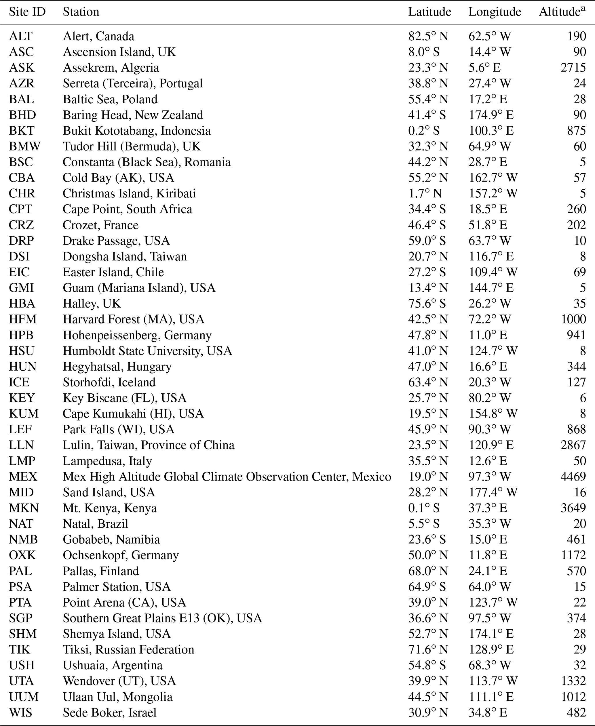
Table 1 Sites of continuous surface measurements used in the inversion and in the reanalysis.

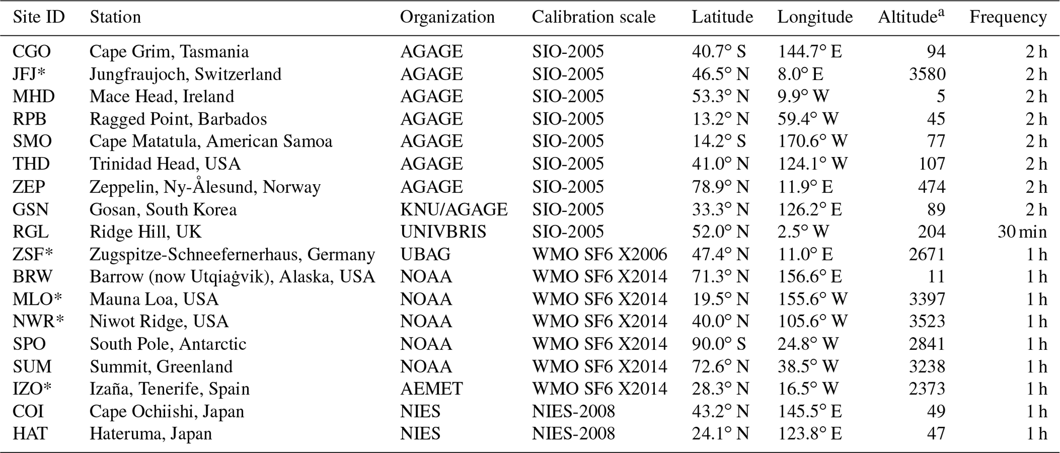
^a The altitude specifies the sampling height in meters above sea level. Stations considered as mountain sites are marked with an asterisk.

The treatment of the baseline is critical when using LPDMs as a basis for atmospheric inversions. Still, it is unclear what influence the choice of a certain baseline approach has on inversion results. Previous studies indicated that different approaches lead to significant mismatches in simulated emissions (Thompson and Stohl, 2014; Henne et al., 2016). However, different methods were never compared systematically and tested for different model setups such as the length of the LPDM backward simulations.

Another problem of LPDM-based inversion studies is the general lack of consistency between regional emission estimates and the global emissions of a GHG. Given that the LPDMs are only usually run backward in time for a few days, the inversions only constrain the emissions in regions where observation stations exist (Rigby et al., 2011). This can lead to substantial deviations of the derived emissions from, often well-known, global totals, a problem shared with regional inversion studies based on Eulerian models.

In this study we (i) investigate the effect of the backward simulation time period within the range of 0–50 d, (ii) analyze the impact of the baseline definition on inversion results, (iii) examine their consistency with known global total emissions, (iv) explore the influence of biases in the baseline and a priori emissions on inversion results for different backward simulation periods, and (v) compare the value of different observation types (flask vs. continuous) for the inversion. We compare three different baseline methods – the REBS method, Stohl's method, and the GDB method – and apply inverse modeling to the species sulfur hexafluoride (SF₆). SF₆ is the most potent GHG regulated under the Kyoto Protocol, with a high global warming potential of approximately 23 500 over a 100-year time horizon (Myhre et al., 2013) and an estimated atmospheric lifetime of 3200 years (Ravishankara et al., 1993). SF₆ is a convenient choice for our studies because it has no negative sources (as, e.g., CO₂), a very long lifetime in the atmosphere, and well-known global emissions, and there are relatively many measurements available. However, we expect our findings to also hold for other species and be informative for inverse modeling of GHGs with LPDMs in general.

2 Methods

2.1 Measurement data

The inversion (Sect. 2.2) is performed using continuous atmospheric observations of SF₆ dry-air mole fractions from 18 observation sites, distributed around the globe. Those measurements were provided by the Advanced Global Atmospheric Gases Experiment (AGAGE; Prinn et al., 2018) network, the NOAA/ESRL halocarbons in situ program (Dutton et al., 2017), and a number of independent organizations, whose data were partly included in the World Data Centre for Greenhouse Gases (WDCGG, 2018). Measurement sites are listed in Table 1, together with acronyms and other station-specific information.

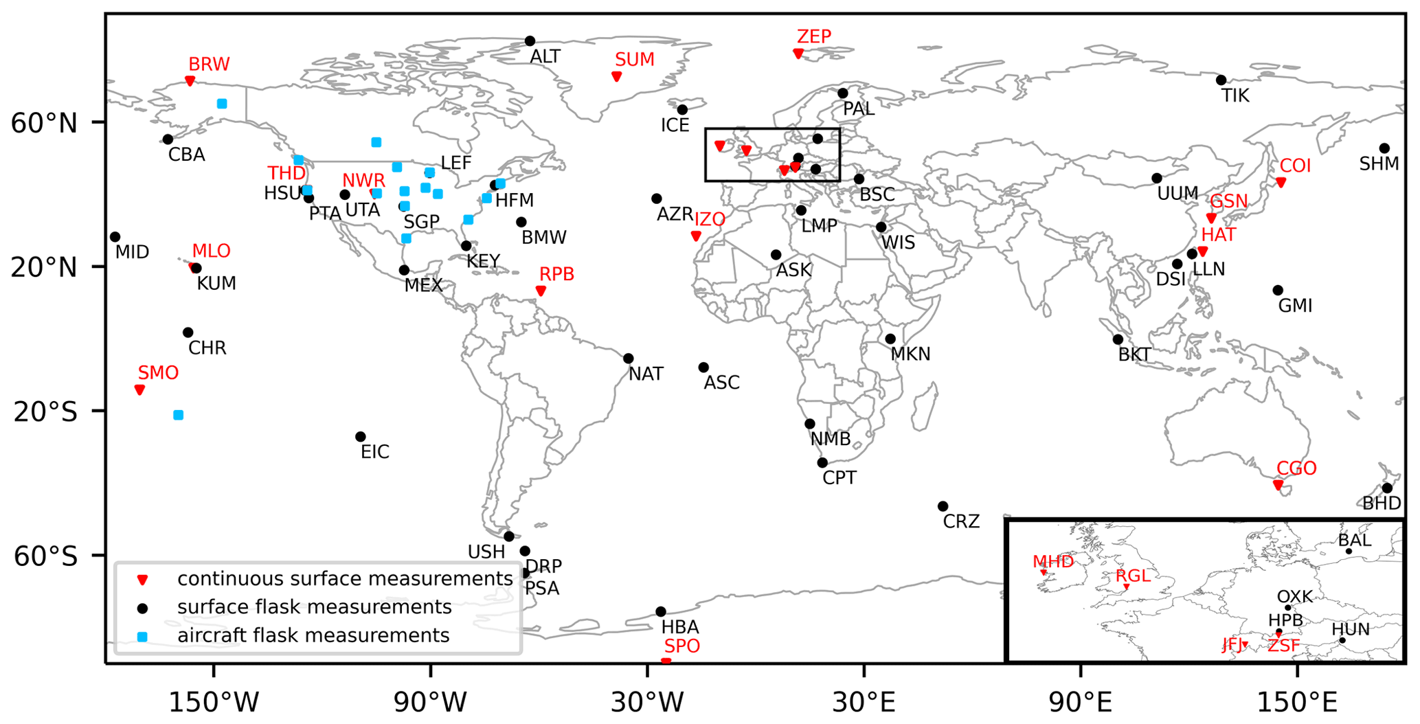
Figure 1 Map of sites with continuous surface measurements used for the inversion (red triangles) and flask measurements (surface: black dots, aircraft: blue squares) that were additionally used for the reanalysis of SF₆.

At AGAGE stations, SF₆ mixing ratios are measured using Medusa gas chromatography followed by mass spectrometry (GC/MS; Miller et al., 2008). At the stations HAT and COI, the SF₆ measurement system is based on cryogenic preconcentration and capillary GC/MS (Yokouchi et al., 2006). At all other stations, gas chromatography followed by electron capture detection (GC-ECD) is used to measure SF₆ mole fractions. Observations were calibrated with four different SF₆ scales: SIO-2005, WMO SF6 X2006, WMO SF6 X2014, and NIES-2008. We converted all observations to the SIO-2005 calibration scale by dividing NIES-2008 calibrated data by the factor 1.013 (Takuya Saito, private communication, 5 February 2021) and WMO SF6 X2014 calibrated data by 1.002 (Guillevic et al., 2018). To convert mole fractions from WMO SF6 X2006 to WMO SF6 X2014, we used $y=a{x}^{\mathrm{2}}+bx+c$, where y corresponds to SF₆ mole fractions on the X2014 scale and x to mole fractions on the X2006 scale. The coefficients a, b, and c have the values of $\mathrm{2.6821}\times {\mathrm{10}}^{-\mathrm{3}}$, $\mathrm{9.7748}\times {\mathrm{10}}^{-\mathrm{1}}$, and $\mathrm{3.5831}\times {\mathrm{10}}^{-\mathrm{2}}$ (NOAA ESRL, 2014), respectively.

We averaged all observation data over 3-hourly intervals. For stations at low altitudes, we selected afternoon values (12:00 to 16:00 LT), to only consider time periods with a well-mixed planetary boundary layer, when the smallest model errors can be expected. At mountain stations, we instead selected observations during nighttime (00:00 to 04:00 LT) to avoid larger errors due to daytime small-scale upslope winds in the complex topography around these sites, which are unresolved in the model. Additionally, we followed a method by Stohl et al. (2009) to identify observations that cannot be brought into agreement with modeled mixing ratios by the inversion, which we removed completely (in contrast to Stohl et al., 2009, who assigned larger uncertainties to these observations). For this, we used the kurtosis of the a posteriori error frequency distribution and iteratively excluded observations causing the largest absolute errors until the kurtosis of the remaining error values fell below 5 (close to a Gaussian distribution). This method removed 0.62 % (63 data points) of the whole dataset, affecting 0 % to 2.92 % of the observations at individual measurement sites. In total, 10 142 observations were used in the inversion for the year 2012.

In order to generate global SF₆ mixing ratio fields required by the GDB method, we performed a 2-year SF₆ reanalysis (for more details see Sect. 2.5), for which we used all the available 2011 and 2012 continuous measurements from the sites listed in Table 1. In addition, we included flask air samples from 44 surface observation stations (NOAA, Dlugokencky et al., 2020) and from 16 aircraft profiling stations (Sweeney et al., 2015; NOAA Carbon Cycle Group ObsPack Team, 2018). Surface flask measurements were available at intervals ranging from a few days up to months. Sampling flights were conducted irregularly with intervals between 2 and 5 weeks at individual sites. Aircraft measurements from individual flights provide vertical SF₆ mixing ratio profiles up to 8.5 km above sea level, where air samples are usually taken within less than an hour. With one exception, all aircraft samples were collected over North America. Additional information about the flask measurements from surface sites and aircraft programs can be found in Tables A1 and A2 (Appendix). All flask measurements were calibrated with the WMO SF6 X2014 calibration scale, and we converted them to the SIO-2005 calibration scale. For the reanalysis, we used 175 557 in situ, 3423 surface flask, and 5581 aircraft measurements amounting to 184 561 measurements in total in 2011 and 2012. Figure 1 provides an overview of all observation sites considered in the inversion and the reanalysis.

In one specific test case (see Sect. 3.2.4), we also used the 2012 surface flask measurements in addition to the continuous measurements for the inversion.

2.2 Inversion method

In this study we use the Bayesian inversion framework FLEXINVERT+, described in detail by Thompson and Stohl (2014), which was further developed since then, to make the code more modular and to include iterative solution methods. However, our results should be valid for all inversion methods based on LPDM calculations, and we thus only include a brief description of FLEXINVERT+. It is based on a linear forward operator H that represents the atmospheric transport, so that the forward problem reads

$$\begin{array}{}\text{(1)}& \mathit{y}=\mathbf{H}\mathit{x}+\mathit{\epsilon },\end{array}$$

where y is the vector of observed mixing ratios, x the emission state vector, and ε the sum of observation and model error. Since H is ill-conditioned and has no unique inverse, a priori emission estimates can be added, in order to solve Eq. (1) for x. The inversion method applies Bayes' theorem to calculate a posteriori emissions, which on the one hand minimize the difference between observed and modeled mixing ratios and on the other hand stay close to the a priori emissions and inside of predefined uncertainty bounds. Assumed uncertainties are Gaussian-distributed, resulting in a minimization of the cost function (e.g., Tarantola, 2005)

$$\begin{array}{}\text{(2)}& \begin{array}{rl}\mathbf{J}\left(\mathit{x}\right)=& {\displaystyle \frac{\mathrm{1}}{\mathrm{2}}}(\mathit{x}-{\mathit{x}}_{\mathrm{p}}{)}^{\mathrm{T}}{\mathbf{B}}^{-\mathrm{1}}(\mathit{x}-{\mathit{x}}_{\mathrm{p}})\\ & +{\displaystyle \frac{\mathrm{1}}{\mathrm{2}}}(\mathbf{H}\mathit{x}-\mathit{y}{)}^{\mathrm{T}}{\mathbf{R}}^{-\mathrm{1}}(\mathbf{H}\mathit{x}-\mathit{y}),\end{array}\end{array}$$

where B is the a priori emission error covariance matrix, R the observation error covariance matrix, and x_p the vector of the a priori emissions. This study uses the following analytical solution to minimize J(x):

$$\begin{array}{}\text{(3)}& \mathit{x}={\mathit{x}}_{\mathrm{p}}+({\mathbf{H}}^{\mathrm{T}}{\mathbf{R}}^{-\mathrm{1}}\mathbf{H}+{\mathbf{B}}^{-\mathrm{1}}{)}^{-\mathrm{1}}{\mathbf{H}}^{\mathrm{T}}{\mathbf{R}}^{-\mathrm{1}}(\mathit{y}-\mathbf{H}{\mathit{x}}_{\mathrm{p}}).\end{array}$$

We use a spatial emission grid (Fig. A1) with 6219 grid cells of varying size ranging from $\mathrm{1}{}^{\circ }\times \mathrm{1}{}^{\circ }$ to $\mathrm{16}{}^{\circ }\times \mathrm{16}{}^{\circ }$. We define the grid by using model information to aggregate grid cells with low emission contributions, as further described by Thompson and Stohl (2014). For this, the emission sensitivity is taken from the LPDM 50 d backward simulation, and the resulting inversion grid is used for all inversions. The output emission fields are saved at a spatial resolution of $\mathrm{1}{}^{\circ }\times \mathrm{1}{}^{\circ }$. x is assumed to not vary with time.

SF₆ has no surface sinks, and its surface fluxes can therefore only be larger than or equal to zero. However, the inversion algorithm can produce negative a posteriori fluxes. To overcome this problem we follow Thompson et al. (2015) and apply an inequality constraint on the a posteriori emissions, using the truncated Gaussian approach by Thacker (2007). This approach, which applies inequality constraints as error-free observations, is described by the following equation:

$$\begin{array}{}\text{(4)}& \widehat{\mathit{x}}=\mathit{x}+{\mathbf{AP}}^{\mathrm{T}}\left({\mathbf{PAP}}^{\mathrm{T}}{)}^{-\mathrm{1}}\right(\mathit{c}-\mathbf{P}\mathit{x}),\end{array}$$

where P is a matrix operator selecting the fluxes violating the inequality constraint, and c a vector of the inequality constraint (zero in our case). x and A represent the a posteriori emissions and error covariance matrix precalculated in the inversion, respectively.

In contrast to many other studies (e.g., Henne et al., 2016; Rigby et al., 2011; Stohl et al., 2009; Thompson and Stohl, 2014), we do not use the option to optimize the baseline mixing ratios in the inversion, except for sensitivity tests. In any case, it is desirable to obtain a baseline that is as accurate as possible prior to any optimization, which is a purely statistical correction that may falsely compensate for errors elsewhere (e.g., in the emissions). Waiving this option further gives us the opportunity to better analyze the differences between investigated baseline methods and to study their impacts on the a posteriori emissions more systematically. For the baseline optimization of the sensitivity tests, we use a temporal window of 28 d and a baseline uncertainty of 0.1 ppt. Increasing the uncertainty up to 0.2 ppt did not show any significant changes in the results. For general details on the baseline optimization, see Thompson and Stohl (2014).

2.3 Atmospheric transport

H is the so-called source–receptor relationship (SRR) in the context of atmospheric transport. The SRR is an emission sensitivity that relates emission changes in a given grid cell to changes in modeled mixing ratios at a given receptor; for further details, see Seibert and Frank (2004). The SRR value in a specific grid cell (units of 1 s m³ kg⁻¹) measures the simulated mixing ratio change at a receptor that a unit strength source (1 $\mathrm{kg}{\mathrm{s}}^{-\mathrm{1}}{\mathrm{m}}^{-\mathrm{3}}$) in that grid cell would create (Stohl et al., 2009).

In this study, we use the LPDM FLEXPART 10.4 (Pisso et al., 2019; Stohl et al., 1998, 2005) to calculate the SRR. The model is run in backward mode as this is more efficient than forward calculations when the number of emission grid cells exceeds the number of observation sites. Available observations are averaged to 3-hourly means (see Sect. 2.1). For each of these means, 50 000 virtual particles are released continuously over the averaging period and followed backward in time. The SRR is calculated by determining the average time the particles spend in each grid cell of the $\mathrm{1}{}^{\circ }\times \mathrm{1}{}^{\circ }$ output grid within the lowest 100 m above the ground, assuming that all emissions occur at or near the ground. FLEXPART is driven by the hourly reanalysis dataset ERA5 (Hersbach et al., 2018) from the European Centre for Medium-Range Weather Forecasts (ECMWF) at a resolution of $\mathrm{0.5}{}^{\circ }\times \mathrm{0.5}{}^{\circ }$ and with 137 vertical levels. Since SF₆ is an almost nonreactive gas, removal processes are neglected in the calculation of the SRR.

In this study, five different backward calculation periods are investigated: 1, 5, 10, 20, and 50 d. At the end of these periods, particles are terminated, and the back trajectories end. Figure 2 shows the 2012 annual average emission sensitivities for the backward calculation period of 5 d (Fig. 2a) and 50 d (Fig. 2b), respectively. On the 5 d timescale large land areas in the Southern Hemisphere (northern Australia, South America, southern Africa) and also parts of the Northern Hemisphere (e.g., India, Iran) are sampled poorly or not at all. In these areas, emissions can therefore not be determined well by the inversion. High sensitivity can only be found at land regions with many receptors, such as Europe. On the 50 d timescale, the SRR has higher values compared to the 5 d backward calculation. Large parts of the Northern Hemisphere are sampled quite well, and the emission sensitivities provide some information, even at areas that are far away from the observation stations. However, emission sensitivities are still low in the tropics, especially over Africa, South America, and northern Australia. Figure 2c shows the increase in the annual averaged SRR due to the use of flask measurements in addition to continuous measurements in the case of 50 d simulations. One can see substantial increases in the vicinity of the measurement sites that quickly decline with distance to the sites. Further SRR values increase in large parts of the Southern Hemisphere; however, the increases over southern continental areas are relatively low, as most flask measurements are not well located for inversion purposes.

Figure 2 Source–receptor relationship obtained from FLEXPART backward simulations, averaged over the year 2012. The SRR is shown for all considered continuous measurement stations and for a simulation period of (a) 5 and (b) 50 d. Panel (c) shows the increase in the annual averaged SRR due to the use of flask measurements in addition to continuous measurements for the case of a 50 d backward simulation period.

2.4 The baseline definition

The transport model can only account for mixing ratio changes caused by emissions within the chosen backward calculation period. Consequently, a baseline representing the influence of all the emission contributions prior to this time period has to be defined.

2.4.1 The REBS method

The REBS method introduced by Ruckstuhl et al. (2012) is a statistical method using a robust local regression model to identify background observations from each individual observation station to estimate a baseline curve. In recent years it has been used in various studies to determine a baseline for atmospheric inversions of several GHG species (e.g., An et al., 2012; Brunner et al., 2017; Henne et al., 2016; Schoenenberger et al., 2018; Simmonds et al., 2016; Vollmer et al., 2016). The REBS method defines observed mixing ratios y(t_i) at each time step t_i as the sum of a baseline signal g(t_i), an enhancement due to polluted air masses m(t_i), and the observational error E_i:

$$\begin{array}{}\text{(5)}& y\left(t_i\right)=g\left(t_i\right)+m\left(t_i\right)+E_i.\end{array}$$

The method assumes that most observations are baseline observations and therefore not influenced during pollution episodes (m(t_i)=0). It also assumes that the baseline curve g is smooth – so that it can be linearly approximated around any given time. The method then applies a local linear regression model that fits the observation data, giving more weight to data points close to the considered time and iteratively excluding data points outside a certain range. An advantage of the REBS method is that it is simple to implement. The code is freely available, and besides some parameters that need to be chosen, it only depends on the observation data. This simplicity, however, also means that the method is unable to take the length of the LPDM backward calculation into account. As we shall see, this leads to systematic biases in the inversion results that depend on the length of the backward calculation. The method also assumes a smoothly varying baseline, which limits its ability to account for meteorological variability. Another disadvantage is the dependence on certain parameter settings. The settings used in this study are provided in Table A3. Finally, the method can only be used at sites with frequent observations, not for flask measurement sites or moving measurement platforms.

2.4.2 Stohl's method

The method introduced by Stohl et al. (2009) is primarily based on the selection of observed mixing ratios at individual observation stations but also uses the simulated SRR values and a priori emissions to determine the baseline. In the last few years, it has been used in several inversion studies (e.g., Brunner et al., 2017; Fang et al., 2014, 2015, 2019; Stohl et al., 2010; Thompson and Stohl, 2014). We apply the method and select the lowest 25 % of observations from individual stations in a moving time window of 30 d to only consider observations which are weakly influenced by emissions within the backward calculation period. Prior simulated mixing ratio enhancements are subtracted from the selected observations to eliminate the emission contributions from within the time interval of the LPDM simulation. In order to avoid an overestimation of their contribution, only the lower half of the prior simulated values and the corresponding observed data points are selected. In every time window, resulting mixing ratios are averaged and finally linearly interpolated to the timestamp of the observations. By subtracting prior simulated mixing ratios, the method takes the length of the LPDM backward calculation into account and aims to avoid an overestimation of the baseline. However, simulated mixing ratios are calculated using a priori emission estimates, making the method dependent on a priori information. Further, the subjective choice of the time window and the subjective selection of observations are problematic. As the REBS method, Stohl's method assumes a smooth baseline curve, and thus it cannot account for sudden changes in the baseline due to meteorological variability. Also, the method can only be used at sites with frequent observations.

2.4.3 The GDB method

The idea of the GDB approach (Thompson and Stohl, 2014) is to determine the baseline directly from a 3D global field of mixing ratios, e.g., from a reanalysis of the atmospheric chemical composition. The end points of the back-trajectories that are used by the LPDM to calculate the SRR are utilized to determine the sensitivity at the receptor to mixing ratios at the points in space and time where particles terminate (see Fig. 3 for a simplified illustration). This sensitivity (termed “termination sensitivity” hereafter) in a particular grid cell is calculated in the LPDM by dividing the number of particles terminating in that cell by the total number released at the receptor, while also including a transmission function to account for loss processes (not relevant for SF₆) during the backward simulation period. The termination sensitivity fields are saved in a 3D $\mathrm{1}{}^{\circ }\times \mathrm{1}{}^{\circ }$ output grid with 16 vertical layers with interface heights at 0.1, 0.5, 1, 2, 3, 4, 5, 7, 9, 12, 15, 20, 25, 30, 40, and 50 km above ground level. For global inversions, baseline mixing ratios are then calculated by multiplying the termination sensitivity with the mixing ratios of the 3D global field and integrating the product over all grid cells. The GDB method can also be used for regional inversions (not done in this study). In this case, the emission contributions from outside the regional domain need to be added to the baseline (Thompson and Stohl, 2014), but otherwise the inversion procedure is identical as described here.

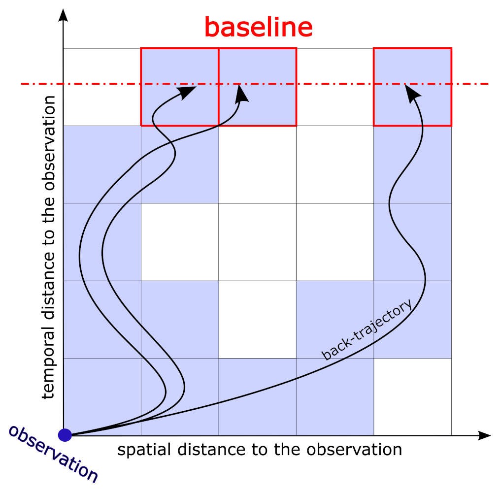
Figure 3 Simplified illustration of the global-distribution-based (GDB) method for baseline determination, where the backward simulation is represented by three back trajectories released at the time and space of a particular observation. The spatiotemporal grid is simplified to two dimensions with a vertical time and a horizontal space axis. Grid cells that contribute to the modeled mixing ratio through emissions are shaded blue; termination grid cells where termination sensitivity is stored are marked with red rectangles; the termination point is illustrated by a dashed red horizontal line.

The GDB method is independent of subjective data selection and choice of parameter settings. In contrast to the REBS method and Stohl's method, it does not assume a smooth baseline and has the potential to fully account for meteorological variability. As illustrated, it excludes emission contributions from within the backward simulation period and therefore provides a baseline that is fully consistent with the length of the backward simulation. Furthermore, contrary to the other two methods, it can also be used at measurement sites with infrequent observations or moving observation platforms. Its accuracy, however, is dependent on the ability to minimize errors and especially biases of the global 3D mixing ratio fields. We target this challenge using the FLEXible PARTicle dispersion chemical transport model (FLEXPART CTM; Henne et al., 2018) to perform a reanalysis of SF₆ as described in the next section.

2.5 Reanalysis of SF₆ using FLEXPART CTM

In this study the LPDM FLEXPART 8-CTM-1.1 is used to perform a reanalysis of SF₆ for the year 2012. It was developed by Henne et al. (2018) and is based on FLEXPART 8.0. Groot Zwaaftink et al. (2018) provide a detailed description of FLEXPART CTM and evaluate this model for the example of CH₄. FLEXPART CTM is run in a domain filling mode where 12 million particles are randomly distributed over the globe, proportional to the air density. In addition to an air tracer, particles also carry the chemical species SF₆. The initialization is based on a latitudinal SF₆ profile based on surface observations. We run the simulation from 2011 to 2012, using 2011 as a spin-up period. Particles are followed forward in time, and whenever a particle resides below the diagnosed boundary layer height, its mass is increased due to surface SF₆ emissions. The model is driven with the ECMWF ERA5 dataset and with emission fields calculated as described in Sect. 2.6. Mixing ratio fields are saved daily on a $\mathrm{3}{}^{\circ }\times \mathrm{2}{}^{\circ }$ output grid and coupled to the backward simulations.

FLEXPART CTM uses a nudging routine to keep simulated SF₆ fields close to the observations of SF₆. With this simple data assimilation method, modeled fields of mixing ratios are relaxed towards observations within so-called nudging kernels around observation sites. For all surface observation stations in the Southern Hemisphere, we assign relatively large uniform kernel sizes, since the model tends to overestimate SF₆ mixing ratios in the Southern Hemisphere, and there are only few measurement stations to correct this bias. For the surface observation sites in the Northern Hemisphere, we assigned smaller kernel sizes to measurement stations with a large observation variability to conserve SF₆ spatial variability, especially over the continents (see Groot Zwaaftink et al., 2018). For the aircraft measurements we predefine vertical levels at 0.05, 0.15, 0.3, 0.5, 0.75, 0.1, 1.5, 2, 2.5, 3, 3.5, 4, 5, 6, 7, 8, and 9 km a.g.l., co-locate the individual measurements to the closest vertical level, and choose kernel sizes that increase with altitude. Specific kernel settings are detailed in Table A4.

2.6 A priori emissions

An a priori estimate of the spatial distribution of SF₆ emissions for the year 2012 is determined by collecting information on the emissions from individual countries. We use country emissions reported to the United Nations Framework Convention on Climate Change (UNFCCC, 2021) and for East Asian countries' emissions estimated by Fang et al. (2014). The sum of these individual country emissions is subtracted from the total global SF₆ emissions determined by Simmonds et al. (2020), and the remaining emissions are distributed to all other countries proportional to their electric power consumption (World Bank, 2021). Finally, total country emissions are disaggregated according to the gridded population density (CIESIN, 2018) within each country's borders. Note at this point that the a priori emissions as constructed agree with recognized global emissions, which should be kept in mind when the global total is used as a reference value in the discussion. The a priori emission uncertainty is estimated to be 50 % in each grid cell, with a minimal value of $\mathrm{1}\times {\mathrm{10}}^{-\mathrm{13}}$ $\mathrm{kg}{\mathrm{m}}^{-\mathrm{2}}{\mathrm{h}}^{-\mathrm{1}}$. Spatial correlation between uncertainties is considered using an exponential decay model with a scale length of 250 km.

3 Results

3.1 Baselines and length of backward simulation

The three investigated baseline methods are discussed for the example of two measurement sites, Gosan and Ragged Point, and for five backward simulation time periods. The Gosan observation station is located on the southwestern tip of Jeju Island, South Korea, monitors the outflows from the Asian continent, and is representative of stations which frequently measure pollution events. The Ragged Point observation station is situated on the eastern edge of Barbados, with direct exposure to the Atlantic Ocean. Ragged Point is primarily influenced by easterly winds providing “clean” background air masses, uninfluenced by local emissions, and is therefore representative of background stations. Both Gosan and Ragged Point periodically intercept air from the Southern Hemisphere and therefore have a rather complex baseline.

Baseline mixing ratios are plotted together with respective observations and a priori mixing ratios for different LPDM backward simulation periods ranging from 1 to 50 d (Figs. 4–7). A priori mixing ratios are calculated as the sum of the baseline and the contribution originating from a priori emissions during the period of the backward simulation (termed “direct emissions contributions” hereafter). Ideally, the choice of the backward simulation period should have no systematic effect on the calculated a priori mixing ratios. By increasing the backward simulation time, and therefore enlarging the temporal domain, additional emission contributions are included in the optimization. Per definition, these contributions are not part of the baseline and should ideally be removed from it. As a result, the baseline should become lower and smoother when the simulation period is increased. We investigate the agreement between modeled and observed mixing ratios for the three methods with time series plots (Figs. 4–7), as well as statistical parameters (bias, mean squared error (MSE), and coefficient of determination (r²)), summarized in Table 2.

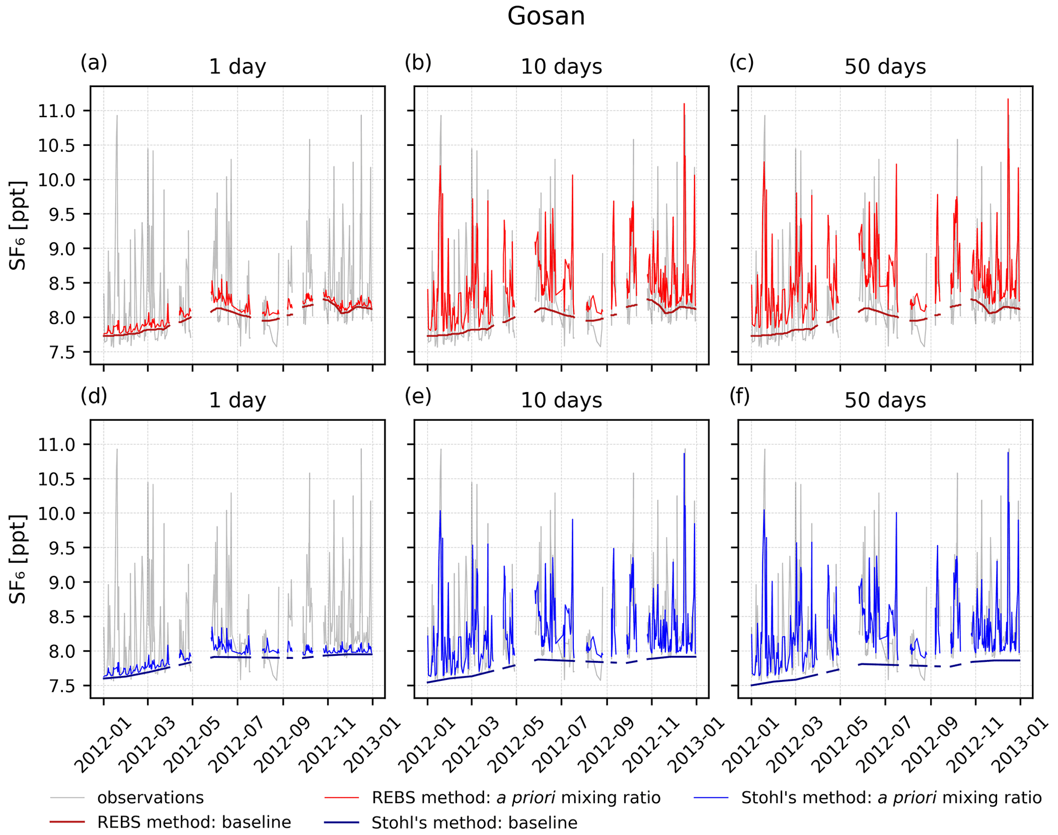
Figure 4 Baseline and a priori SF₆ mixing ratios calculated with the REBS method (panels a–c) and Stohl's method (panels d–f) at the Gosan observation station, compared to SF₆ observations. Model results are shown for backward simulations of 1 d (panels a and d), 10 d (panels b and e), and 50 d (panels c and f).

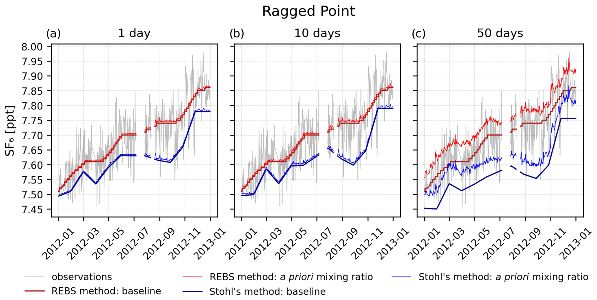
Figure 5 Baseline and a priori SF₆ mixing ratios determined by the REBS method and Stohl's method at the Ragged Point observation station for backward simulation times of 1 d (panel a), 10 d (b), and 50 d (c).

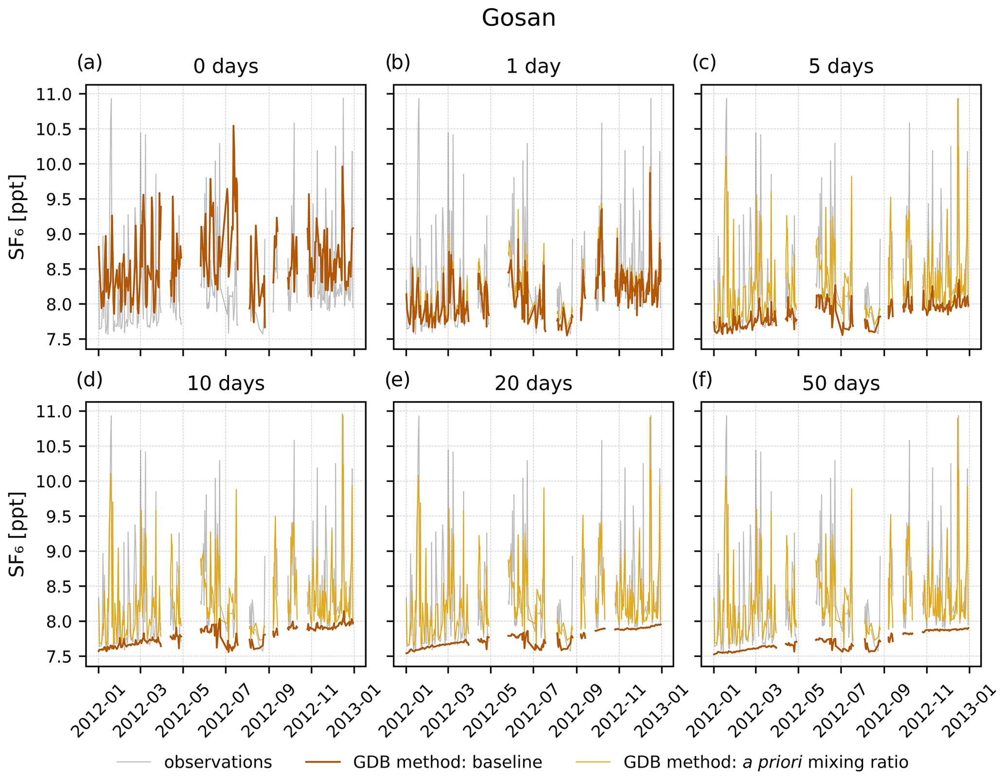
Figure 6 Baseline and a priori SF₆ mixing ratios calculated with the GDB method at the Gosan observation station for backward simulation times of 0 (panel a), 1 (b), 5 (c), 10 (d), 20 (e), and 50 d (f).

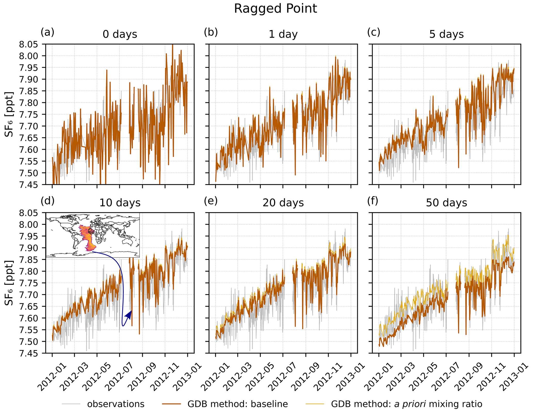
Figure 7 Baseline and a priori SF₆ mixing ratios calculated with the GDB method at the Ragged Point measurement station for backward simulation periods of 0 (panel a), 1 (b), 5 (c), 10 (d), 20 (e), and 50 d (f). The inset in panel (d) shows the termination sensitivity averaged over all heights for the time of the marked observation low point, illustrating the method's ability to account for baseline changes due to episodic transport from the Southern Hemisphere.

Table 2 Bias, mean squared error (MSE), and coefficient of determination (r²) of a priori SF₆ mixing ratios determined by the three investigated baseline methods with respect to observed mixing ratios. Statistical parameters are shown for three different backward calculation periods (1, 10, and 50 d) at the stations Gosan and Ragged Point. Also reported are the bias, MSE, and r², calculated separately for all stations listed in Table 1 and then averaged.

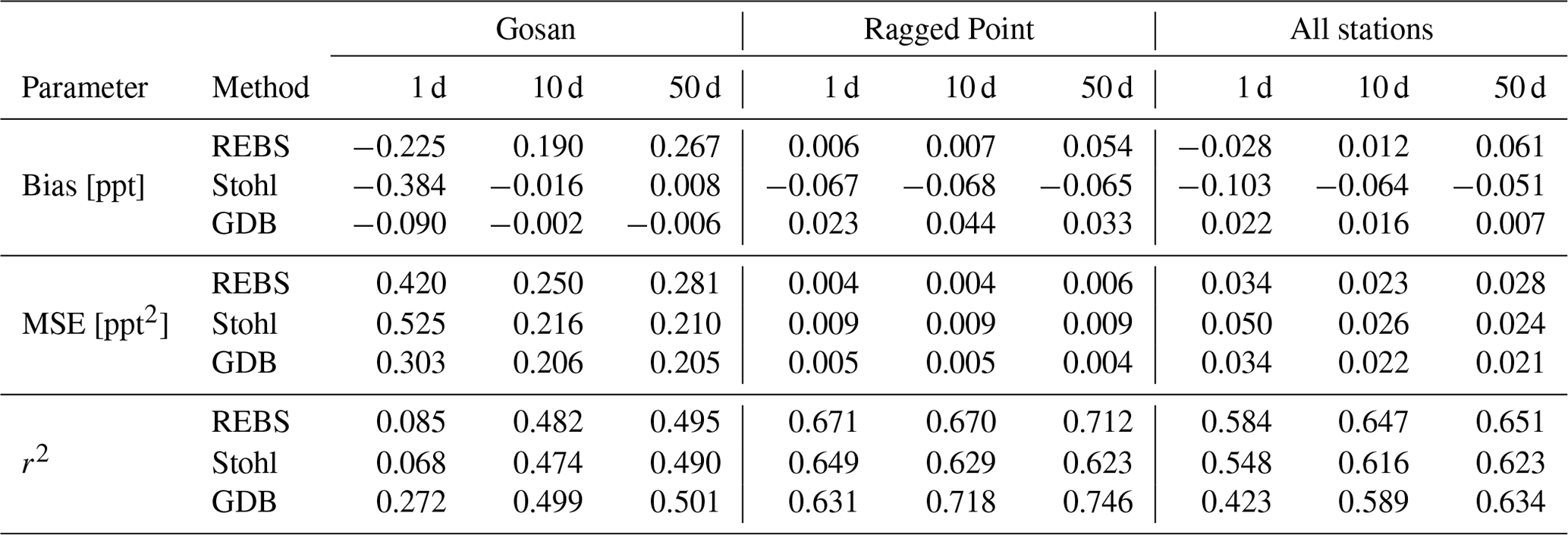
Figure 4 shows the smooth baselines calculated with the REBS method and Stohl's method at the measurement station Gosan. In the case of 1 d backward simulations (Fig. 4a and d), both methods show a poor agreement between modeled and observed mixing ratios, as neither the smooth baselines nor the small direct emission contributions can reproduce the observed mixing ratios during pollution episodes. This agreement becomes much better with longer backward simulation periods (Fig. 4b and e). The REBS baseline stays completely unchanged for different backward simulation periods. Therefore, a priori mixing ratios grow with increasing simulation periods (Fig. 4b and c), as more direct emissions contribute to the calculated total mixing ratio. For Gosan, the bias is negative for the 1 d simulation period but becomes increasingly positive for longer simulation periods (Table 2). This systematically increasing bias is inherent to all purely observation-based baseline methods and cannot be corrected without adding model information. In contrast, Stohl's baseline level decreases with longer backward simulation periods as higher direct emission contributions are subtracted from the preselected observations. Consequently, the bias of the a priori mixing ratios changes less between 10 and 50 d of backward simulation (Fig. 4e and f). This is confirmed by statistical parameters in Table 2 also showing only little change between 10 and 50 d.

At Ragged Point (Fig. 5), the a priori mixing ratios determined by the REBS method fit the observation data very well for short backward simulation periods, where baseline and a priori mixing ratios overlap because of small direct emission contributions (Fig. 5a and b). This is expected, since the method determines the baseline by fitting the observation data while iteratively excluding outliers. Since regional pollution events captured at Ragged Point tend to be very small, no significant measurement peaks need to be excluded. Therefore, the REBS baseline fits well through the measurement data, resulting in a good statistical model–observation agreement (Table 2). However, the smooth baseline is unable to reproduce the observed variability. In the case of a simulation period of 50 d (Fig. 5c), more direct emission contributions give higher a priori mixing ratios, overestimating the measurements and causing a large bias. In contrast, due to its 25th percentile preselection of observations, Stohl's method shifts the baseline curve towards the lowest observations. In the case of Ragged Point, these lowest observations come from southern hemispheric air masses. Hence, Stohl's baseline is more representative of southern hemispheric conditions, which do not necessarily dominate at that site. Consequently, a priori mixing ratios underestimate the observations for low direct emission contributions (Fig. 5a and b). The resulting bias is almost unaffected by the different backward simulation periods (Table 2 and Fig. 5c), showing the method's ability to compensate for increasing direct emission contributions. However, the rather ad hoc 25th percentile preselection of data for the baseline is obviously not justified for a background station with few pollution episodes and southern hemispheric air interceptions, leading to a systematic underestimation of modeled a priori mixing ratios, irrespective of the length of the backward simulation.

The GDB method is illustrated for all backward simulation periods tested, including a case without any backward simulation (0 d). In this extreme case, the baseline is obtained directly from the value of the global mixing ratio field simulated with FLEXPART CTM in the spatiotemporal grid cell of the respective observation. At Gosan, FLEXPART CTM reproduces observed mixing ratios well, even capturing a few pollution events (Fig. 6a). This good agreement is however expected, since these observations were used for the nudging in the FLEXPART CTM model. In the 1 d backward simulation case (Fig. 6b), the method computes a highly variable baseline, partly representing the observed variability. This results in a much better agreement between a priori and observed mixing ratios than using the REBS method or Stohl's method (Table 2). The GDB baseline becomes smoother and lower with increasing backward simulation time. The loss of variability arises from the fact that the GDB method calculates the baseline from a weighted average of grid cell mixing ratios at the trajectory termination points. The longer particles are followed backward in time, the more widely dispersed over large geographical regions termination points become, thus resulting in a smoother baseline. The lowering of the GDB baseline is compensated for by the increase of the direct emission contributions (see Sect. 2.4.3 and Fig. 3), ensuring a seamless transition between forward (FLEXPART CTM) and backward simulations. As a result, a priori mixing ratios in Fig. 6 show no large systematic changes with an increasing simulation period between 5 and 50 d.

Figure 6 also demonstrates the advantage of the Lagrangian backward simulation. As FLEXPART CTM is limited in resolution and particle number, it can only reproduce a few pollution events at Gosan, and it underestimates the highest and overestimates the lowest measured SF₆ mixing ratios, as demonstrated in the 0 d case (Fig. 6a). The backward simulation is initiated at the exact location of the measurement point and provides much higher resolution (Fig. 6b–f). If the backward calculation period is long enough that back trajectories reach important emission regions, mixing ratio spikes similar to the observed ones can be simulated. At the same time, the lowered baseline for intrusions of southern air masses during the Asian summer monsoon also allows the lowest observed values to be captured. Table 2 shows exclusively improving correlation between modeled and observed values with increasing backward simulation periods.

Figure 7 illustrates the GDB method at the Ragged Point station. FLEXPART CTM (Fig. 7a) reproduces the measured mixing ratios well. However, it generates more variability than observed at this station. This is partly due to the limited number of particles in the domain-filling simulation, which introduces noise into the model results. This is averaged out by the GDB method with increasing backward simulation time, as the baseline becomes a weighted average over many grid cells. Nevertheless, the baseline maintains variability for all tested simulation periods, fitting the observed signal well (Fig. 7b–e). It is noteworthy that at Ragged Point a substantial part of the observed SF₆ variability seems to be caused by transport from different latitudes/regions without direct emission contributions, exemplified by the quite variable baseline even for the 50 d backward simulation. In contrast, the direct emissions accumulated over the 50 d of the backward simulation are producing an almost constant enhancement over the baseline. This is very different from a station like Gosan that is strongly influenced by pollution episodes.

Notice also that for backward simulation times of 10 d and longer, the GDB method is able to reproduce short episodes of very low observed mixing ratios at Ragged Point that are caused by episodic transport from the Southern Hemisphere (see also inset in Fig. 7d). Neither the REBS method nor Stohl's method could correctly reproduce these negative SF₆ excursions.

Additional figures illustrating the three baseline methods at all investigated measurement sites can be found in the Supplement. Despite all the advantages of the GDB method, it does not work well if the modeled global mixing ratio fields are biased. At Mace Head and Zeppelin (see Figs. S17 and S33 in the Supplement), FLEXPART CTM overestimates the measurements, and thus the GDB method gives a baseline that partly exceeds the observations. Possible error sources include deficiencies in the emission assumptions driving the model that are impossible to be compensated for through nudging with the few available observations. It is also unclear whether the FLEXPART CTM nudging routine was able to properly correct mixing ratios at higher altitudes, as aircraft measurements were available only over North America (with one exception). On the other hand, statistical baseline methods might work better at observation stations, where the baseline termination is less complex. At Mace Head (Fig. S18 in the Supplement) for instance, both the REBS method and Stohl's method lead to a very high correlation between modeled and observed mixing ratios for the case of a 50 d backward simulation (r²=0.87). Nevertheless, for the REBS method, the discussed growing negative bias with longer simulation periods can be observed.

Statistical parameters (bias, MSE, and r²) were separately calculated for every observation station, and respective averages over all stations are shown in Table 2. One should keep in mind that the REBS method and Stohl's method are directly based on the observations themselves, and thus the dependency between observed and modeled a priori mixing ratios is likely higher than in the case of the GDB method, where observations are rather used to improve the mixing ratio fields. Therefore, it is remarkable that overall the GDB method obtains smaller bias and MSE values than the other two methods. The REBS method shows the highest r² values. The main reason for this good correlation is that the method captures the trend in the time series very well, which represents a considerable fraction of the total variability in the data. The GDB baseline may contain a fair fraction of noise, in contrast to the smooth baselines of the other two methods. This will lead to lower correlation. However, it is noteworthy that for the GDB method, the r² value improves systematically with growing backward simulation time and for 50 d even exceeds the value derived by Stohl's method. By extending the backward calculation period from 10 to 50 d, the GDB r² value increases by 0.045, meaning that an extra 4.5 % of the observed variability can be explained by the model. Notice also the improvement in bias and MSE, which can be observed for the GDB method and Stohl's method, when extending the simulation period from 10 to 50 d. The REBS method does not show these improvements due to its systematical increase of bias with backward simulation time.

3.2 Inversion results

Figure 8 illustrates (a) the global distribution of the SF₆ a priori emissions 2012 as well as (b–d) the emission increments (i.e., a posteriori minus a priori emissions) for the three investigated baseline methods using SRRs from 20 d backward calculations. A priori emissions are allocated to regions proportional to electricity use and population density. This implies large a priori emissions in South and East Asia, including China, which is estimated to be the biggest contributor to global SF₆ emissions. In general, much higher a priori emissions are allocated to the Northern Hemisphere than to the Southern Hemisphere. We should also note that the emission optimization of the inversion focuses on regions with large a priori emissions, where also assumed uncertainties are bigger (see Sect. 2.6), assigning more freedom to the algorithm.

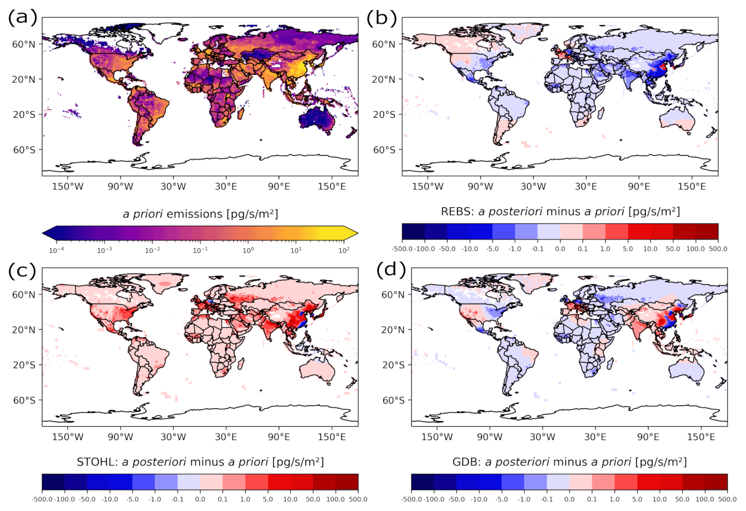
Figure 8 A priori SF₆ emissions (a) and SF₆ emission increments given by the inversion when using the REBS method (b), Stohl's method (c), and the GDB method (d) based on 20 d LPDM backward simulations.

The inversion increments in Fig. 8b–d show three very contrasting pictures, illustrating the huge impact of the choice of the baseline method on the inversion results. Using different baseline approaches completely changes the results of the inversions. When using the REBS method (Fig. 8b), the inversion produces negative emission increments in almost all areas of the globe. As the real emissions are unknown, this is not necessarily an unrealistic result. However, when considering these mostly negative increments together with the discussed positive bias for REBS baselines in Table 2 (especially for longer backward simulation periods), there is reason to assume that the REBS method overestimates baselines and consequently underestimates the a posteriori emissions overall. In contrast, the inversion algorithm produces positive increments almost everywhere around the globe when applying Stohl's method (Fig. 8c). Again, considering this together with the discussed negative biases in Table 2, this might indicate an underestimation of the baselines and an overestimation of the a posteriori emissions overall. In the case of the GDB method (Fig. 8d), negative and positive increments are more balanced. Overall, the patterns are more similar to the ones of the REBS method, except in East Asia, where they rather resemble the patterns of Stohl's method. Large positive increments can be seen in East Asian regions and parts of Europe, whereas the inversion tends to produce slightly negative increments in the Southern Hemisphere.

National emissions

As the verification of emission reports to UNFCCC takes place on a national scale, the impact of baseline methods on national emissions is of great interest (Fig. 9). In countries with very low emission sensitivity (e.g., Brazil), inversion increments are very small in all three cases, and therefore the baseline choice has little impact. However, considering countries with higher emission sensitivities (e.g., China), the a posteriori emissions are very sensitive to the baseline definition. In almost all cases, the REBS method leads to smaller national emissions and Stohl's method to larger national emissions than the GDB method. Due to the large emissions in China, the differences in a posteriori emissions become especially apparent there, with almost a factor of 3 emission difference, corresponding to almost 30 % of the 2012 global SF₆ emissions.

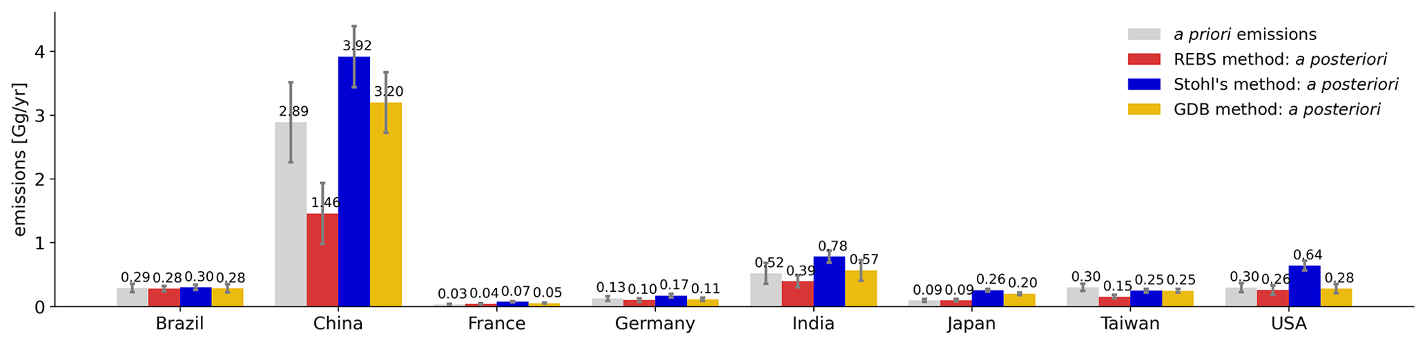
Figure 9 National SF₆ emissions for selected countries, based on 20 d LPDM backward calculations with different choices of the baseline method. Uncertainties represent a 1σ range.

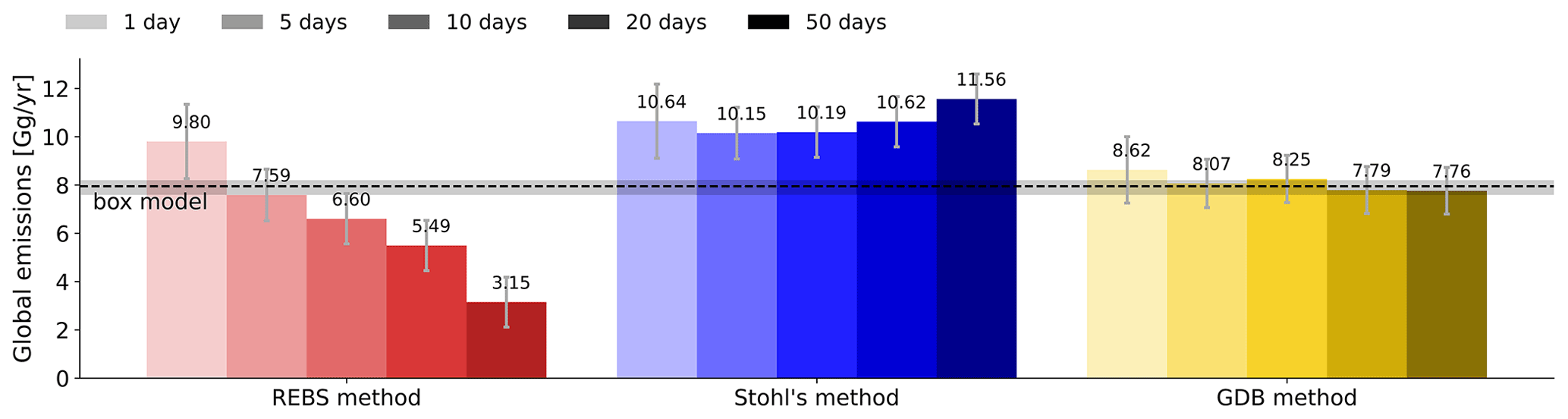
Figure 10 SF₆ global emissions derived by the inversions. Results are shown for the three applied baseline methods and for the five applied backward simulation periods between 1 and 50 d. The horizontal dashed line represents the reference value of the AGAGE 12-box model with shaded error bands. Uncertainties represent a 1σ range.

Global emissions

The 2012 SF₆ global emissions are shown in Fig. 10. The bars represent inversion results using different backward calculation periods between 1 and 50 d (light to dark shading). The horizontal dashed line illustrates a reference value calculated by Simmonds et al. (2020) with the AGAGE 12-box model. Notice that this is the same value used to calculate the a priori emissions, so the line also represents the global a priori emissions, which should be kept in mind for the interpretation of the results. Since the uncertainty of the global emissions is relatively small, global emissions derived by the inversion should roughly match the value of the box model, regardless of which backward simulation period was used.

For the REBS method, calculated global emissions (red) decrease dramatically with growing backward simulation time, showing values between 3.15 and 9.80 Gg yr⁻¹. This is a consequence of the method's incapability to remove emission contributions from the baseline when the backward simulation period expands, leading to a systematical overestimation of the baseline and underestimation of the emissions. The resulting bias increases with growing simulation period, and as a result global emissions estimates deviate strongly from the box model.

In the case of Stohl's method (blue), derived global emissions do not show such a systematic decrease with longer backward simulation periods as observed for the REBS method. This is because Stohl's method not only selects low mixing ratio observations, but also uses model information to maintain the baseline. For longer backward simulation periods, higher simulated mixing ratios are subtracted from the preselected observations to compensate for more direct emission contributions. Nevertheless, global emissions significantly exceed the reference value of the box model for all applied simulation periods, implying a systematic overestimation of emissions through too low baselines. The overestimation of the global emissions increases with longer backward simulation times larger than 5 d. This suggests that the method overcompensates for additional direct emission contributions when the simulation period expands, subtracting values that are systematically too high from the preselected observations.

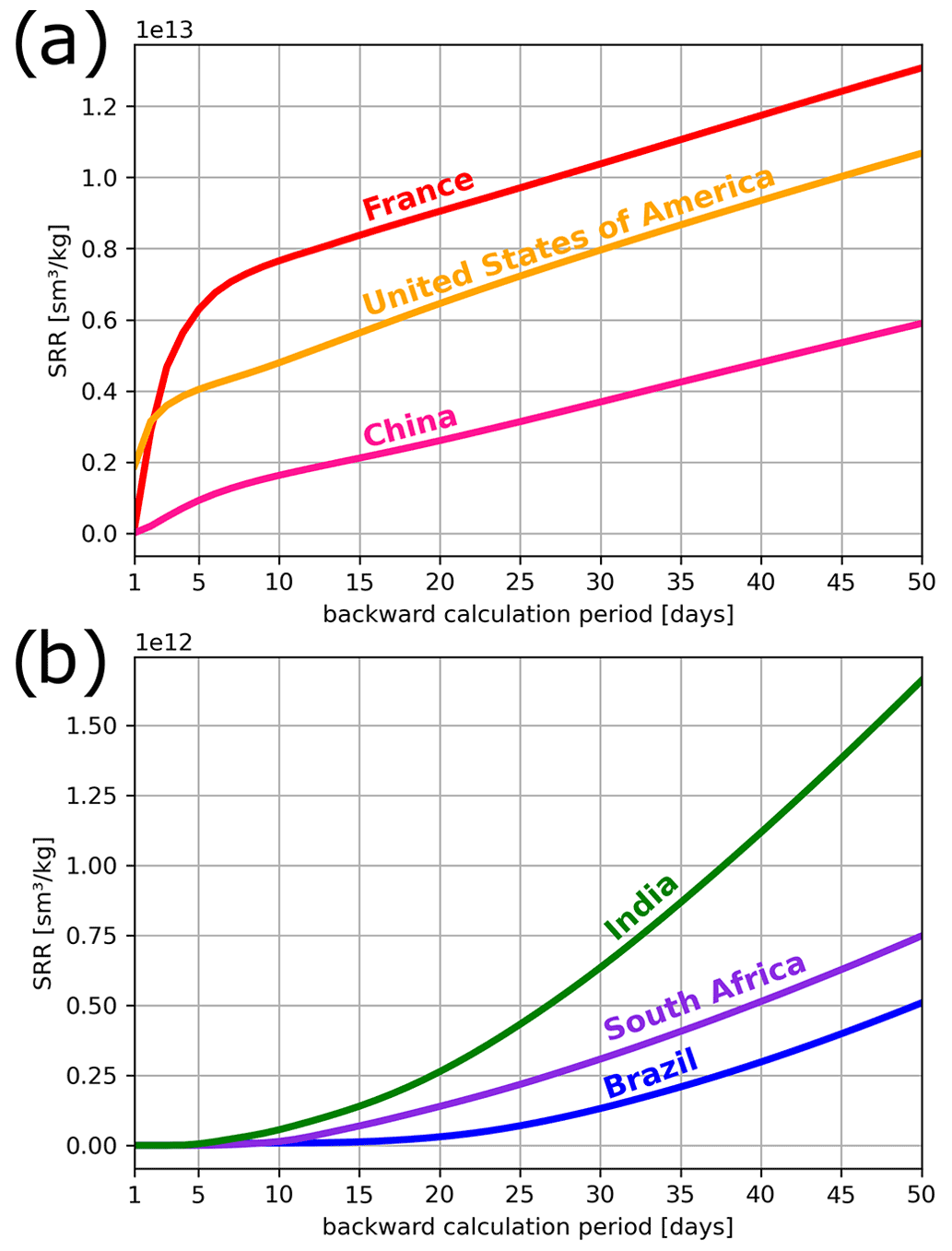
Figure 11 SRR for individual countries and different backward calculation periods between 1 to 50 d, considering all continuous measurement stations in Table 1. The values shown are averages over the grid cells of (a) France, USA, and China and (b) India, South Africa, and Brazil for the year 2012.

We further investigate whether the encountered biases can be reduced by optimizing the baseline in the inversion. Therefore, we repeated the inversion with exactly the same setup, except optimizing the REBS baseline and Stohl's baseline as part of the inversion. Results are shown in Fig. A2. In the case of the REBS method, the baseline optimization only has little effect on the global total a posteriori emissions for backward simulation periods between 1 and 10 d and only becomes noticeable after 20 d. The greatest improvements can be observed for the 50 d simulation, where the bias is almost halved. Still, for longer simulation periods the increasing improvements through the baseline optimization cannot compensate for the growing underestimation of the emissions and substantial biases remain. Optimizing Stohl's baseline shows great improvements, especially for longer simulation periods. These improvements increase systematically with growing backward simulation period, and results get very close to the box model outcome for the 20 and 50 d simulation case.

Considering the inversion results based on the GDB method, global emissions are in good agreement with the box model result for all tested backward simulation periods, as the global a posteriori emissions stay close to the global a priori value. Furthermore, these global emissions stay almost unchanged for different backward simulation periods, demonstrating the method's ability to adjust the baseline according to the sampled emissions of different simulation periods.

The advantage of longer backward simulation periods

As an argument for a relatively short backward simulation period, Stohl et al. (2009) stated that “the value for the inversion of every additional simulation day decreases rapidly with time backward”. Certainly, this is true for countries and regions that are well covered by the global monitoring network. For instance, for France the SRR increases rapidly in the first few backward simulation days but flattens to a linear increase for longer backward simulation periods (Fig. 11a). A similar behavior can be observed for many countries in the Northern Hemisphere, although the curve's slope for the first few days varies. For countries poorly covered by the monitoring network, however, the SRR is close to zero for the first 5 to 15 backward days, and only longer backward simulations might provide information for the inversion (see Fig. 11b). For these countries, the SRR increase with time only flattens to a linear increase for very long transport times, even beyond the 50 d used in this study.

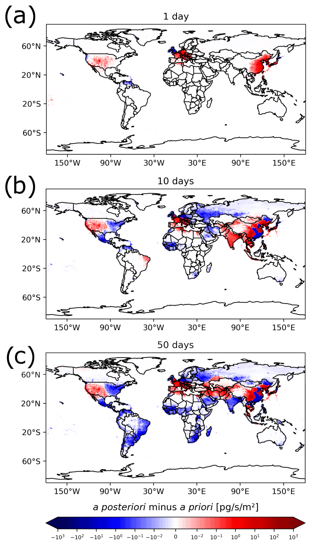
Figure 12 SF₆ emission increments calculated with the inversion by using the GDB method and a backward simulation period of (a) 1, (b) 10, and (c) 50 d.

Figure 12 further illustrates the impact of different backward simulation periods on the inversion, by showing emission increments for the GDB method and for backward simulation periods of 1, 10, and 50 d. In the case of 1 d backward calculations (Fig. 12a), the inversion only significantly optimizes a priori emissions in East Asia and parts of Europe. As the backward simulation period is extended to 10 d (Fig. 12b), the inversion optimizes emissions in larger parts of the Northern Hemisphere, but in the Southern Hemisphere emission increments are still small. In the case of 50 d (Fig. 12c), the inversion optimizes emissions even far away from observation stations (e.g., South America or South Africa). In India, where SRR values are also small, and a priori emissions (and thus emission uncertainties) are high (see also Fig. 11b), the emission increments even switch from positive to negative by extending the period from 10 to 50 d. Also, the calculated relative uncertainty reduction increases by extending the backward simulation period (see Fig. A3a–c).

The use of flask samples

An advantage of the GDB method is the possibility to include flask measurements from fixed sites or moving platforms in the inversion. By contrast, the REBS method and Stohl's method require short measurement intervals at fixed sites for the statistical baseline calculation. Here, the baseline could be taken from nearby or same latitude continuous sites or represented through baselines at the domain border in case of regional inversions (Manning et al., 2021). Figure 13a shows the relative change in a posteriori emissions and Fig. 13b the additional relative error reduction when using flask measurements additionally to the continuous measurements for the 50 d backward simulation. One can see substantial differences in the USA, eastern Europe, South Africa, East Asia, and the Near East, where also an additional error reduction occurs. While this additional error reduction can be relatively large (up to 73 %) for grid cells in the vicinity of the measurement sites, it quickly decreases down to a few percent with larger distance to the measurements. Consequently, flask measurements only show a small influence on the total global emission estimate (<1 %) but can have a large impact on calculated national emissions of specific countries (Fig. A4). For countries in the Near East, the additional use of flask measurements changes national emission estimates by 40 % to 100 %. South African and American emissions are modified by around 10 %.

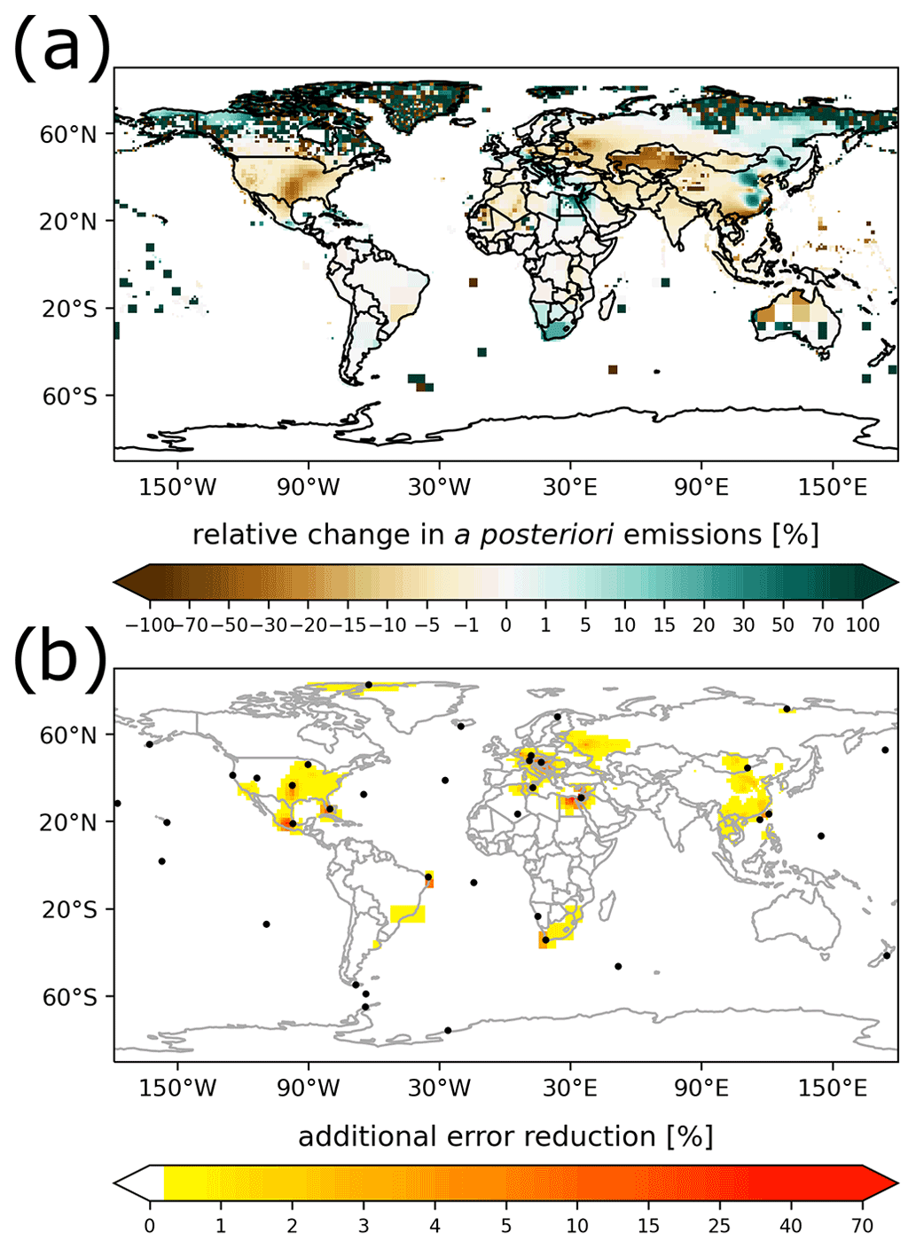
Figure 13 (a) Relative change in a posteriori emissions and (b) the additional error reduction when using flask measurements in addition to continuous measurements for the 50 d simulation. The locations of the flask measurements are marked with black dots.

Reliable global emissions can only be obtained with long backward simulation periods

In previous sections, we have used global mixing ratio fields from the GDB method, where great care has been taken to avoid biases that would affect the baseline, and we have used global a priori emissions that correspond to the rather well-known global SF₆ emissions. These are optimal conditions for the inversion that are rarely fulfilled for other species than SF₆. For many species, global emissions are less well known, and with fewer observations than for SF₆ the global distribution (and, thus, the baseline) is also more uncertain. However, a skillful inversion should tolerate such biases and still produce reliable results. While we lack information for verifying that regional emissions are reliable, for SF₆ we can at least test whether global emissions can be determined by our inversion in the presence of biases.

Figure 14 shows global a posteriori emissions when biases in (1) the a priori emissions and (2) global mixing ratio fields were added. This is shown for different backward simulation periods between 1 and 50 d and for the 50 d case with the inclusion of flask measurements. Note that for all these sensitivity cases shown in Fig. 14, we use the same absolute a priori emission uncertainties as for the original a priori emissions without any artificial bias.

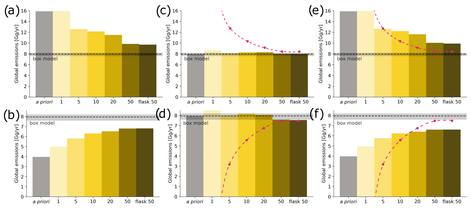
Figure 14 Global SF₆ emissions using the GDB method shown for different sensitivity cases, using backward simulation periods between 1 and 50 d and a 50 d backward simulation case in which flask measurements were also included in the inversion in addition to continuous measurements. The sensitivity cases include (a) doubled and (b) halved a priori emissions; biased global mixing ratio fields with a uniform bias of (c) −0.003 and (d) +0.003 ppt in every grid cell; and combinations of the two test types; (e) doubled a priori emissions plus −0.003 ppt global field bias; (f) halved a priori emissions plus +0.003 ppt global field bias. The dashed pink lines represent the expected relationship between the baseline bias and a resulting emission bias if a global box model was used and the bias attributed solely to emissions in different periods corresponding to the backward simulation times.

Comparing the inversion results for doubled (Fig. 14a) and halved (Fig. 14b) a priori emissions clearly shows that the corresponding biases in the global a posteriori emissions are reduced substantially with increasing backward simulation period and converge towards the rather well-known global SF₆ emission from the box model. It seems an extension of the backward simulation period beyond 50 d would be required in order to further reduce the remaining bias. The inclusion of flask measurements leads to slight additional improvements.

Another sensitivity test was performed with artificially biased global mixing ratio fields by subtracting (Fig. 14c) or adding (Fig. 14d) 0.003 ppt from/to the FLEXPART CTM model output in every grid cell of the 3D mixing ratio fields. 0.003 ppt is equivalent to roughly 1 % of the 2012 global mixing ratio increase and thus corresponds to about 3 d of global SF₆ emissions. To still fit the model to the observations, the inversion will try to compensate for such a bias in the baseline with a bias of the opposite sign in the emissions. As always, the inversion can only attribute this additional bias to emissions within the simulation period. Therefore, shorter backward simulation periods require a greater modification of emissions than longer periods, in order to compensate for the baseline bias. To fully compensate for the baseline bias equivalent to 3 d of emissions, global a posteriori emissions would need to deviate strongly from the reference value for the 1 d case but converge towards it with increasing backward simulation time. This is shown by the dashed pink line, which indicates the expected relationship between this baseline bias and a resulting emission bias if a global box model was used and the bias attributed solely to emissions in different periods corresponding to the backward simulation times. In fact, with a positive baseline bias, negative emissions would be required for backward simulation times of less than 3 d, as the baseline exceeds the observations. The inversion results do not show this extreme behavior, since for short backward simulation times high SRR values are only found in small regions, and the emission changes there are bound by the prescribed a priori uncertainties. Notice that in our case of a known added bias, this is rather a shortcoming, as this shows that the inversion is not able to compensate for the baseline bias for short backward simulation times. Only for the longest times do the emissions converge towards the expected global emissions (dashed pink lines), and only for such long backward simulation times do baseline biases equivalent to 3 d of emissions become negligible. We also investigated the inversion behavior for larger baseline biases, subtracting/adding (Fig. A5a and b) 0.05 ppt from/to the global fields, corresponding to roughly 50 d of the 2012 global SF₆ emissions. Here again, the results for short simulation times seem unpredictable; i.e., they do not follow the described expected behavior, indicated by the dashed pink lines. Only for the 50 d simulation periods do results converge to the expected global emissions, consistent with the respective baseline bias.

Finally, we also combined doubled a priori emissions with a −0.003 ppt bias in the global mixing ratio fields (Fig. 14e) and halved a priori emissions with a +0.003 ppt bias (Fig. 14f). For both cases, the inversion becomes less sensitive to biases in the a priori emissions and the global fields with longer backward simulation periods.

Final remark

In this study, we show many advantages of using relatively long backward simulation periods for the inversion. Nevertheless, the improvement of regional emission patterns is still limited by the observation network. A lack of observations in one region cannot simply be compensated for by extending the simulations for stations in other regions to very long periods. For backward simulation times of 20–50 d, the emission sensitivity is distributed over large areas but usually still concentrated within broad latitude bands. The additional information to be gained from such long simulation times, on top of the information provided by the shorter simulation times, can probably best be compared with the inversions done with a multi-box model such as the AGAGE 12-box model (e.g., Rigby et al., 2013), which is capable of determining the emissions in broad latitude bands. Consequently, if the emissions in certain regions with a dense observation network are already well constrained by shorter simulation periods, the residual emission will be attributed correctly as an emission total to all other regions of the same latitude band with a poor station coverage. The effective resolution of the obtained emissions in such data-poor regions may be very coarse, but the result might still be informative. Furthermore, the emission sensitivity for the 20–50 d backward period is still not uniformly distributed over a latitude band and thus provides some limited regional information. Perhaps supported with a limited number of strategically located flask measurements, inversions with long backward simulation times could provide coarse but robust information on emissions in poorly sampled regions. Independently, the growing correlation between modeled and observed mixing ratios with increasing backward simulation length (Table 2; averaged over all stations) also shows that longer backward simulations hold additional information, even though the information gain decreases with every day added to the simulation length and probably becomes marginal for very long backward simulation times. However, we propose to make use of this additional information and apply longer periods whenever possible to make the best use of the existing observation network.

4 Conclusions

We have examined the use of LPDMs for inverse modeling of GHG emissions by varying the backward simulation period in the range of 1 to 50 d, testing several methods for estimating a baseline, investigating the influence of biases in the a priori emissions and the baseline, and exploring the value of flask measurements for the inversion. We found the following:

• A baseline method that is purely based on the observations at the observation site itself, such as the REBS method, may lead to unreliable inversion results that are highly sensitive to the length of the LPDM backward simulation and can lead to unrealistic a posteriori global total emissions. For instance, for the year 2012, inversions with the REBS method produce a posteriori global total SF₆ emissions ranging between 9.8 and 3.2 Gg yr⁻¹ for backward simulation periods between 1 and 50 d, compared to a well-known reference value of around 8.0 Gg yr⁻¹. Optimizing the baseline shows little effect for simulation periods between 1 and 20 d but could halve the bias in the 50 d simulation case. Although the improvements of the baseline optimization increase with growing backward simulation period, the simultaneously growing bias cannot be compensated for.

• A baseline method that is based on the observations at the site itself but corrects for emissions occurring during the LPDM backward simulation period leads to smaller sensitivity to the backward calculation time but may still lead to substantially biased emissions irrespective of the backward simulation period. For instance, inversions with Stohl's method overestimate the well-known 2012 SF₆ global total emissions by 2.2–3.6 Gg yr⁻¹ (28 %–45 %). Optimizing the baseline, however, shows great improvements, especially for longer simulation periods.

• A global-distribution-based (GDB) approach, where the LPDM backward simulation is nested into a global mixing ratio field, leads to a posteriori emissions that are less sensitive to LPDM backward calculation lengths and stay close to the global total emission value. In contrast to station-specific baselines, the GDB method allows for the inclusion of low-frequency measurements (e.g., flask samples) or data from mobile platforms into the inversion.

• Statistical comparisons of a priori modeled versus observed mixing ratios suggest that longer LPDM backward simulations outperform shorter simulations. In particular, extending the trajectory length from 5–10 to 50 d can reduce the mean squared error and increase the correlation.

• Inverse modeling is highly sensitive to biases in the a priori emissions as well as biases in the baseline. We could show that this sensitivity can decrease with the length of the backward simulation period, and we find that longer backward simulation periods can help to correct biased global emission fields. In the presented case, it is not possible to correct strongly biased global a priori emissions with backward simulation periods of 1–10 d, while they are captured quite accurately with 50 d backward simulations.

• The additional use of flask measurements has the potential to improve the observational constraint on SF₆ emissions, especially close to the measurement sites. However, existing flask sampling sites are often not well located for inversion purposes. Similar to Weiss et al. (2021), we suggest that placing a few additional flask sampling sites downwind of potential emission regions in currently undersampled parts of the world (in particular, tropical South America, tropical Africa, India, Australia, and the Maritime Continent) would have disproportionately large value in improving regional and global a posteriori emission fields.

Following these results, we advise against the use of baseline methods that are purely based on the observations of individual sites. At least great care needs to be taken that problems such as those demonstrated in this paper do not occur. In order to reduce biases, the optimization of the baseline as part of the inversion might be necessary but would likely not be sufficient to avoid biases completely. We recommend also employing longer LPDM backward simulation periods, beyond 5–10 d, as this can lead to improvements in overall model performance, can produce more robust global emission estimates, and might help to constrain emissions, at least at a very coarse resolution, in regions poorly covered by the monitoring network. When consistency between regional and global emission estimates is important, even longer backward simulation periods than 50 d may be useful. Finally, we suggest taking additional flask measurements at continental sites in the tropics and the Southern Hemisphere as they would greatly enhance inversion-derived global emission fields.

Appendix A

Table A1 Surface flask measurement sites.

^a The altitude specifies the sampling height in meters above sea level.

Table A2 Aircraft flask measurement programs.

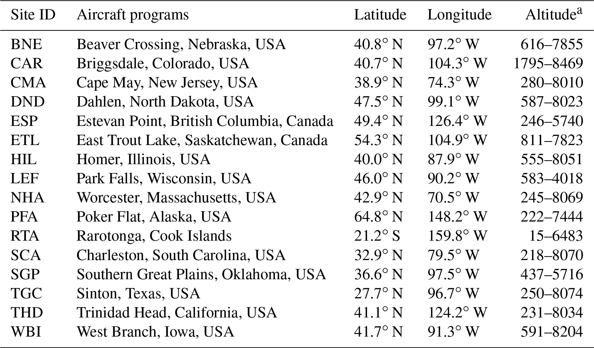
^a The altitude specifies the range of sampling heights in meters above sea level.

Table A3 Setting parameters of the REBS method. For more information, see Ruckstuhl et al. (2012).

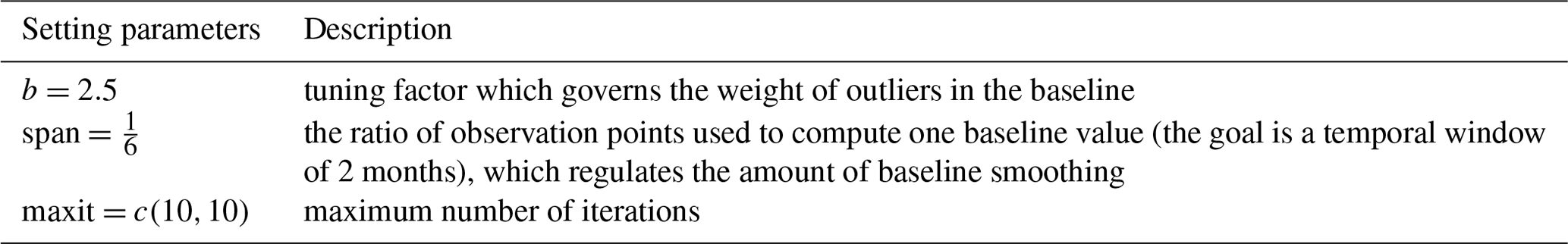
Table A4 Nudging kernel settings for surface and aircraft measurement sites. The kernels are set to have an equal spatial length (in m) in the x and the y direction. For surface measurement sites in the Northern Hemisphere, an upper limit for h_y was set to 25^∘; σ_obs defines the standard deviation of measurements over the simulation period at each nudging location; σ_max describes the maximum value of σ_obs from all surface observation stations. For aircraft measurement sites, the kernel size depends on the height level above ground H. For additional information on the parameters, see Groot Zwaaftink et al. (2018).

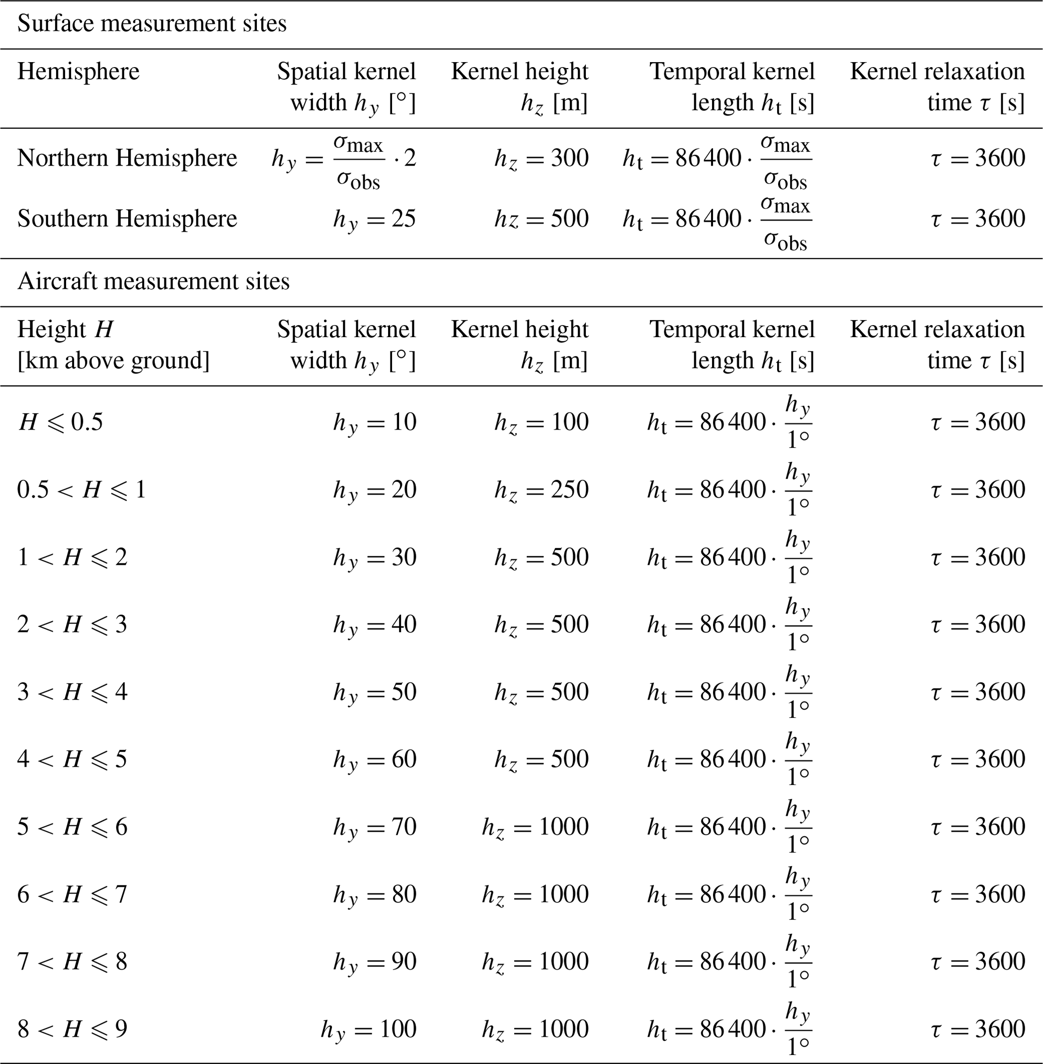
Figure A1 Variable-resolution grid on which emissions are optimized by the inversion.

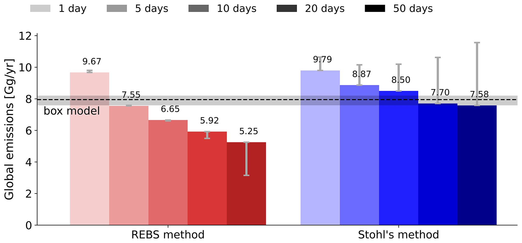
Figure A2 Calculated SF₆ global emissions when baseline concentrations are optimized as part of the inversion. Grey bars represent the improvements obtained by the baseline optimization. Results are shown for the REBS method and Stohl's method and for all five applied simulation periods between 1 and 50 d. The horizontal dashed line represents the reference value of the AGAGE 12-box model with shaded error bands.

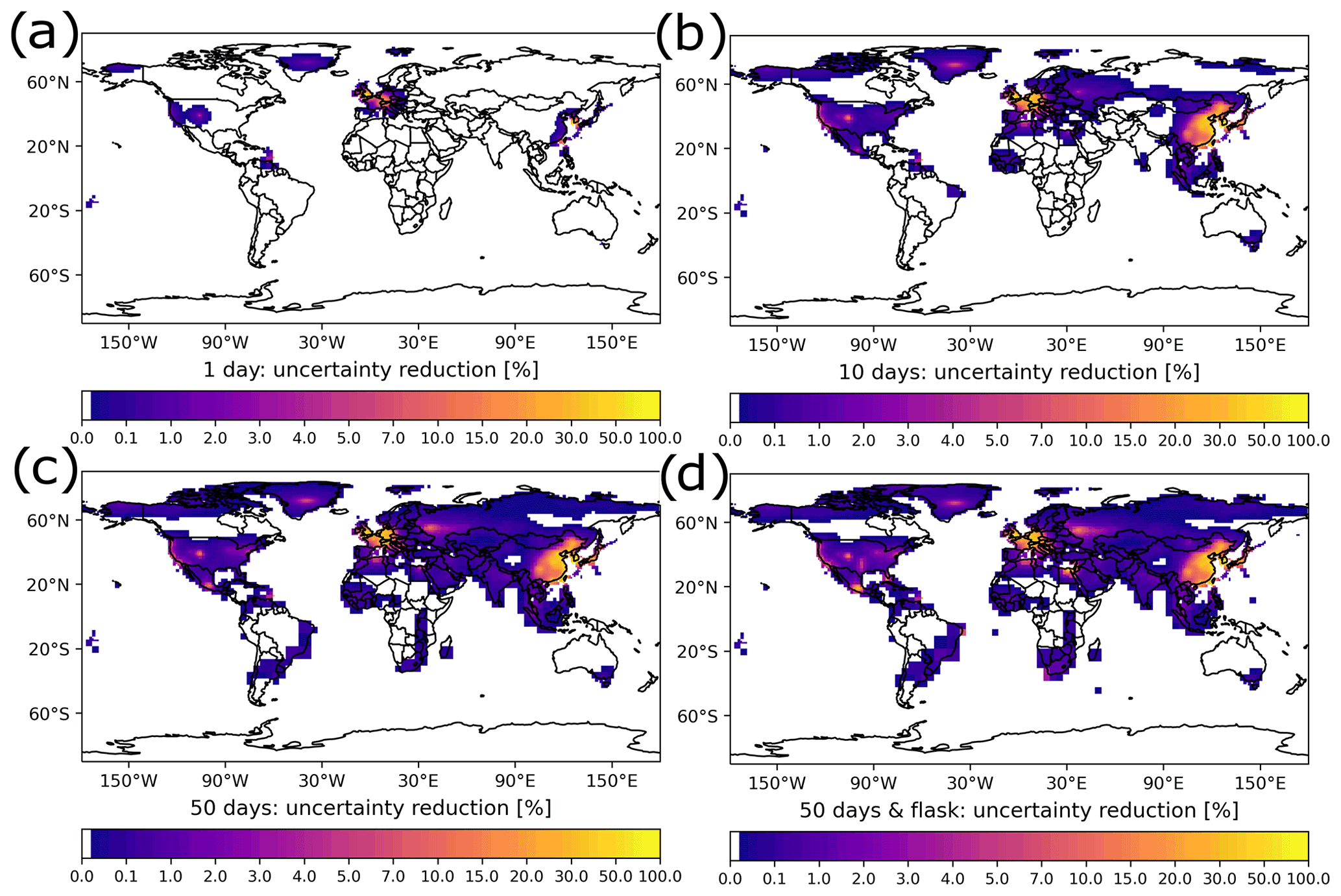
Figure A3 Relative uncertainty reductions ($\mathrm{1}-u_{\text{post}}/u_{\text{pri}}$) calculated with the inversion by using the GDB method and a backward simulation period for (a) 1, (b) 10, and (c) 50 d and (d) for the 50 d case in which flask measurements were also included.

Figure A4 Relative change in national a posteriori emissions of selected countries, when flask measurements are used in addition to continuous measurements in the case of 50 d simulations.

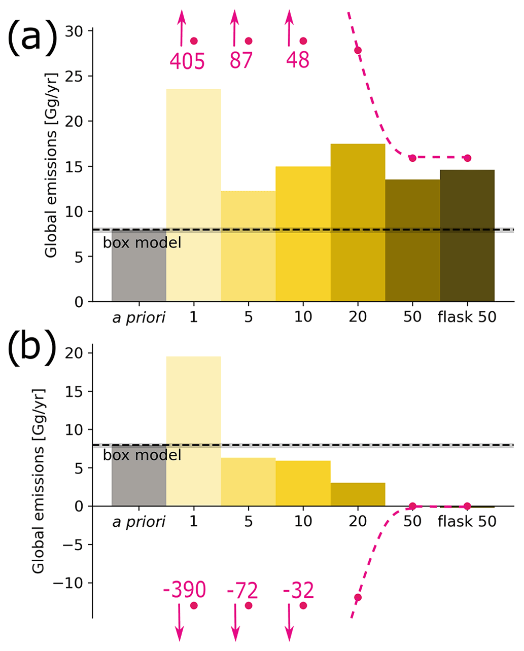
Figure A5 Global SF₆ emissions using the GDB method shown for two sensitivity tests, where a uniform bias of (a) −0.05 and (b) +0.05 ppt is added to every grid cell of the global mixing ratio fields. Results are shown for backward simulation periods between 1 and 50 d, and for a 50 d backward simulation case, where additionally to continuous measurements also flask measurements were included in the inversion. The dashed pink lines represent the expected relationship between the baseline bias and a resulting emission bias if a global box model was used and the bias attributed solely to emissions in different periods. For these two sensitivity tests, a priori uncertainties were set to 500 %.