the Creative Commons Attribution 4.0 License.
the Creative Commons Attribution 4.0 License.
 | 17 Nov 2022
Impact of increased resolution on the representation of the Canary upwelling system in climate models
Adama Sylla
Emilia Sanchez Gomez
Juliette Mignot
Jorge López-Parages
We investigate the representation of the Canary upwelling system (CUS) in six global coupled climate models operated at high and standard resolution as part of the High Resolution Model Intercomparison Project (HighResMIP). The models' performance in reproducing the observed CUS is assessed in terms of various upwelling indices based on sea surface temperature (SST), wind stress, and sea surface height, focusing on the effect of increasing model spatial resolution. Our analysis shows that possible improvement in upwelling representation due to the increased spatial resolution depends on the subdomain of the CUS considered. Strikingly, along the Iberian Peninsula region, which is the northernmost part of the CUS, the models show lower skill at higher resolution compared to their corresponding lower-resolution version in both components for all the indices analyzed in this study. In contrast, over the southernmost part of the CUS, from the north of Morocco to the Senegalese coast, the high-ocean- and high-atmosphere-resolution models simulate a more realistic upwelling than the standard-resolution models, which largely differ from the range of observational estimates. These results suggest that increasing resolution is not a sufficient condition to obtain a systematic improvement in the simulation of the upwelling phenomena as represented by the indices considered here, and other model improvements notably in terms of the physical parameterizations may also play a role.
- Article
(7772 KB) - Full-text XML
- BibTeX
- EndNote


The upwelling is an upward motion of seawater from intermediate depths toward the ocean surface resulting from the friction of the surface wind on the ocean surface. Upwelled water masses are colder and richer in nutrients than the surface waters they replace. Therefore, upwelling zones correspond to areas of very productive marine ecosystems and high fish resources (Herbland and Voituriez, 1974; Minas et al., 1982; Huyer, 1983; and Tretkoff, 2011). In areas where the upwelling occurs along the coast, this phenomenon presents a noticeable socio-economic importance for the countries concerned, in particular in relation to the fishery sector (Gómez-Gesteira et al., 2008). From a physical point of view, coastal upwelling is mainly caused by prevailing trade winds blowing equatorward parallel to the coastline, which push the surface waters away from the coast through the so-called Ekman transport. As a result, the divergent flow at the surface is compensated by an onshore flow from below that brings colder and nutrient-rich waters to the surface. In addition, positive divergent oceanic circulation may also be triggered at the surface by a cyclonic wind stress curl. Indeed, in the eastern subtropical basins, where trade winds tend to slow down near the coast, the wind drop-off induces a cyclonic wind stress curl that also contributes to upwelling (Pickett, 2003; Capet et al., 2004; and Bravo et al., 2016). This second effect is associated with the so-called Ekman pumping, and it acts to side up deeper waters into the euphotic zone. Both offshore Ekman transport and Ekman pumping contribute to enhance the nutrients levels in leading to an enhanced biological production along the coast (Pennington et al., 2006). There are four major coastal upwelling systems (hereafter EBUSs for eastern boundary upwelling systems) in the global ocean: the Canary, Benguela, Humboldt, and California systems. These areas cover less than 1 % of the global ocean surface, but they contribute more than 20 % of the global fish catches (Pauly and Christensen, 1995).
Among the four EBUSs mentioned above, we focus here on the Canary upwelling system (CUS), which extends from the northern tip of the Iberian Peninsula at 43∘ N to the south of Senegal at about 10∘ N (Fig. 1). The variability in this upwelling system has been studied on a seasonal timescale (Torres, 2003, and Alvarez et al., 2005). It has also been studied on longer timescales, but to a lesser extent, due to the lack of sufficiently long, continuous time series (Blanton et al., 1987). In the CUS, the strength of the upwelling-favorable winds is associated with latitudinal variation in the Intertropical Convergence Zone (ITCZ) and the Azores high-pressure system, which are both part of the Hadley circulation. The Azores high pressure migrates from 25∘ N in late winter and 35∘ N in late summer. The Azores High drives both the intensity and the latitudinal extension of the northeasterly winds along the CUS (Wooster et al., 1976; Van Camp et al., 1991; Mittelstaedt, 1991; Nykjær and Van Camp, 1994; and Benazzouz et al., 2014).
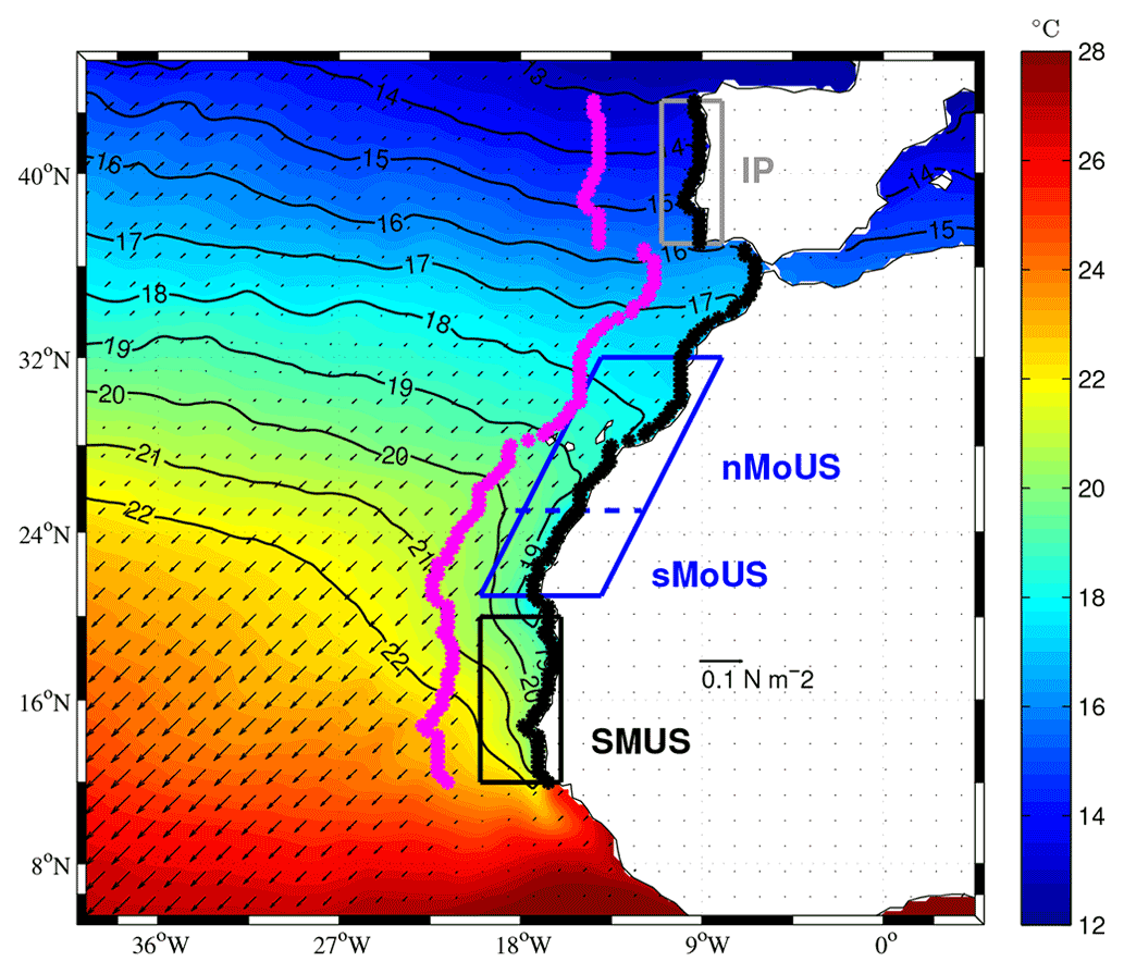
Figure 1Colors: OISSTv2 climatological mean (∘C) in March averaged over the 1992–2011 period. Black vectors show the wind stress from the Cross-Calibrated Multi-Platform (CCMP; computed offline from winds as described in the Appendix). The referent vector is shown inland, and the contours show some SST values. The gray box (37–43∘ N, 8–11∘ W) represents the Iberian Peninsula region (IP); the black box (12–20∘ N, 16–20∘ W) represents the Senegalo–Mauritanian subregion (SMUS). The inclined blue box outlines the Morocco (MoUS) subdomain (21–32∘ N), with a dashed blue line representing the northern boundary of the southern Morocco subdomain (sMoUS). The stars indicate the coastal (black) and offshore (magenta) locations used for the computation of the thermal upwelling index (see Sect. 2.3). The black and magenta dots are separated by 5∘ of longitude.
According to previous studies, the CUS can be divided into different sub-systems based on its circulation, physical environment, and shelf dynamics (Santos et al., 2005; Gómez-Gesteira et al., 2008; and Arístegui et al., 2009). The western coast of the Iberian Peninsula (hereinafter IP), located between 37 and 43∘ N, is the northern limit of the CUS. The IP presents a discontinuity in the flow with the northwestern African coast (Arístegui et al., 2004). This is caused by the presence of the Strait of Gibraltar, which allows the exchange of water between the Mediterranean Sea and the Atlantic Ocean. Upwelling activity along the western coast of the IP occurs during boreal summer due to the poleward migration of the Azores High, which leads to northerly winds flowing along the coast (Wooster et al., 1976; Fraga, 1981; Blanton et al., 1984; Bakun and Nelson, 1991; Gomez-Gesteira et al., 2006; deCastro et al., 2008a; Alvarez et al., 2008; and Pires et al., 2013). Furthermore, the narrow shelves of the IP coast result in lower annual biological productivity than in the other subregions of the CUS (Arístegui et al., 2009). In the area surrounding the Gibraltar Strait (from latitude 33 to 36∘ N), the upwelling is drastically reduced.
The Morocco upwelling system (hereinafter MoUS), located from 21 to 32∘ N, is the central part of the CUS. According to several studies the MoUS can be divided into two subdomains: the northern part (nMoUS) and the southern part (sMoUS), extending between 26–32∘ N and 21–25∘ N respectively (Santos et al., 2005; Gómez-Gesteira et al., 2008; and Arístegui et al., 2009). In the nMoUS, upwelling occurs during the boreal summer, while the sMoUS is one of the few locations in the world where upwelling is persistent throughout the year. This permanent upwelling is due to the fact that, unlike in the case of the other subregions within the CUS, in the sMoUS the prevailing winds are always parallel to the coastal line and blowing equatorward.
Finally, in the southern part of the CUS, the Senegalo–Mauritanian upwelling system (SMUS), which extends from 12 to 20∘ N, is the southernmost part of the CUS. Here the upwelling occurs from November to May, when the ITCZ reaches its southernmost position (Faye et al., 2015, and Sylla et al., 2019).
In the last decades, the sensitivity of EBUSs to climate change has received increasing attention (Bakun, 1990; McGregor et al., 2007; and Barton et al., 2013). Improving our knowledge of the response of the CUS to global warming is of crucial importance since the food resources and economy of neighboring countries greatly depend on its characteristics and evolution in the coming decades. By using the averages of the meridional wind stress component derived from ship reports, Bakun (1990) suggested that coastal upwelling intensification would occur in response to continued global warming. Specifically, he argued that anthropogenic climate change air temperatures on the continents are expected to rise more than in the adjacent oceans (Manabe et al., 1991), producing a deepening of the thermal low-pressure systems over land, which lead to an intensification of the land–sea sea level pressure gradients and a subsequent increase in summertime upwelling-favorable winds (Rykaczewski et al., 2015). Efforts to test Bakun's hypothesis of upwelling intensification under the recent warming trend are challenged by the limited spatial and temporal extent of observations (Cardone et al., 1990). In this context, climate models offer an alternative method to simulate large-scale representation of the CUS and its sensitivity to increased greenhouse gas concentration. By using upwelling indices based on wind stress and/or sea surface temperatures (SSTs), Wang et al. (2015) and Sylla et al. (2019) show that climate models, such as those participating in the Coupled Model Intercomparison Phase (CMIP) exercises, are able to capture the main characteristics of the EBUSs. According to Pickett (2003), the success of these low-resolution estimates of coastal upwelling may depend on their implicit integration of both near-shore Ekman transport and offshore Ekman pumping. Nevertheless, standard-resolution global climate models suffer from several limitations as they do not represent finer-scale processes associated with the upwelling, in particular the structure of the offshore wind stress divergence and curl (Small et al., 2015, and Vazquez et al., 2019, and references therein). Indeed, most coupled climate models incorrectly simulate various processes occurring in these regions and suffer from warm SST biases (Richter, 2015). Misrepresentation of stratocumulus clouds has been identified as one of the primary reasons for this bias. Model inability to produce stratocumulus decks can lead to absorption of excessive shortwave radiation in the upper ocean and anomalously warm SSTs, which in turn induces a positive feedback to the initial error (Richter, 2015, and Zuidema et al., 2016). Further, model resolution and errors in surface winds could also play a role through their impact on turbulent fluxes, coastal upwelling, and offshore Ekman transport (Gent et al., 2010; Richter, 2015; Zuidema et al., 2016; and Ma et al., 2019). Most coupled climate models suffer from warm biases, in SST and wind, near the subtropical eastern boundary regions (Davey et al., 2002; Richter and Xie, 2008; and Richter et al., 2012). Despite numerous improvements in models over time, these problems have persisted because of their coarser resolution. However increasing model resolution leads to an improvement in the upwelling representation; in particular the SST warm biases over the upwelling regions are reduced (Small et al., 2015). Some works have concluded that model resolution influences the overall representation of the mean climate over the tropical Atlantic (Doi et al., 2012, and Exarchou et al., 2018) and the tropical North Atlantic response to remote forcings such as El Niño–Southern Oscillation (ENSO; López-Parages and Terray, 2022). In line with these studies, Gent et al. (2010) report that an increase in the nominal resolution of the atmospheric grid from 2 to 0.5∘ lowers SST biases up to 60 % within the major upwelling areas. Harlass et al. (2015) found that a significant improvement of warm biases within the Tropical Atlantic can be reached with a simultaneous refinement of the horizontal and vertical resolutions of the atmospheric grid. Small et al. (2015) claimed that a good representation of the upwelling systems such as the Benguela (coastal upwelling along the southern African coast) requires an eddy-resolving ocean model and an atmospheric model with enough resolution () to realistically capture the wind stress curl over the eastern boundary of the tropical Atlantic Ocean.
Thus in the last few years, modeling centers have made a great effort to develop higher-resolution global climate models. The recent CMIP6 exercise coordinated the High Resolution Model Intercomparison Project (HighResMIP/PRIMAVERA), aiming to assess the benefits of increased resolution in climate models (Haarsma et al., 2016). Climate model resolution was drastically increased in the atmospheric and oceanic components, and for the first time a coordinated protocol was proposed to assess the impact of enhanced model resolution in the representation of the climate system. This is a topic of growing interest, particularly as some recent simulations suggest improvements in both large-scale aspects of the atmospheric and ocean circulation and in small-scale processes and climate extremes (Haarsma et al., 2016; Roberts et al., 2016; Vanniere et al., 2019; and Hewitt et al., 2020). So far, the effects of increased CMIP6 model resolution on the upwelling systems have still not been assessed. Here, we provide the first detailed analysis of the potential benefits of increasing model resolution in simulating the CUS. To this aim, we compare the model performance in representing the upwelling indices defined in Sylla et al. (2019) by using the standard- and high-resolution versions of some of the climate models that participated in the CMIP6 HighResMIP project. The upwelling indices used in this study are based on SST and wind stress. The SST index aims at describing the surface thermal signature of the CUS upwelling. Although this is a simplified view of the upwelling, this index has the advantage of being based on a well-observed variable so that it can be properly constrained by observations. The other three indices used here are based on the surface wind stress and meridional gradients of sea level. They aim to quantify key mechanisms implicated in the generation of upwelling vertical velocities: coastal divergence of the Ekman transport, Ekman pumping, and possible counteracting effects due to convergences of the geostrophic flow.
The paper is organized as follows: Sect. 2 describes the numerical experiments, the observational and reanalysis data sets, and the different metrics used in this study. Section 3 provides a characterization of the upwelling in observations, while the role of the model resolution in simulating the CUS is assessed in Sect. 4. Finally, results are discussed, and a conclusion is provided in Sect. 5.
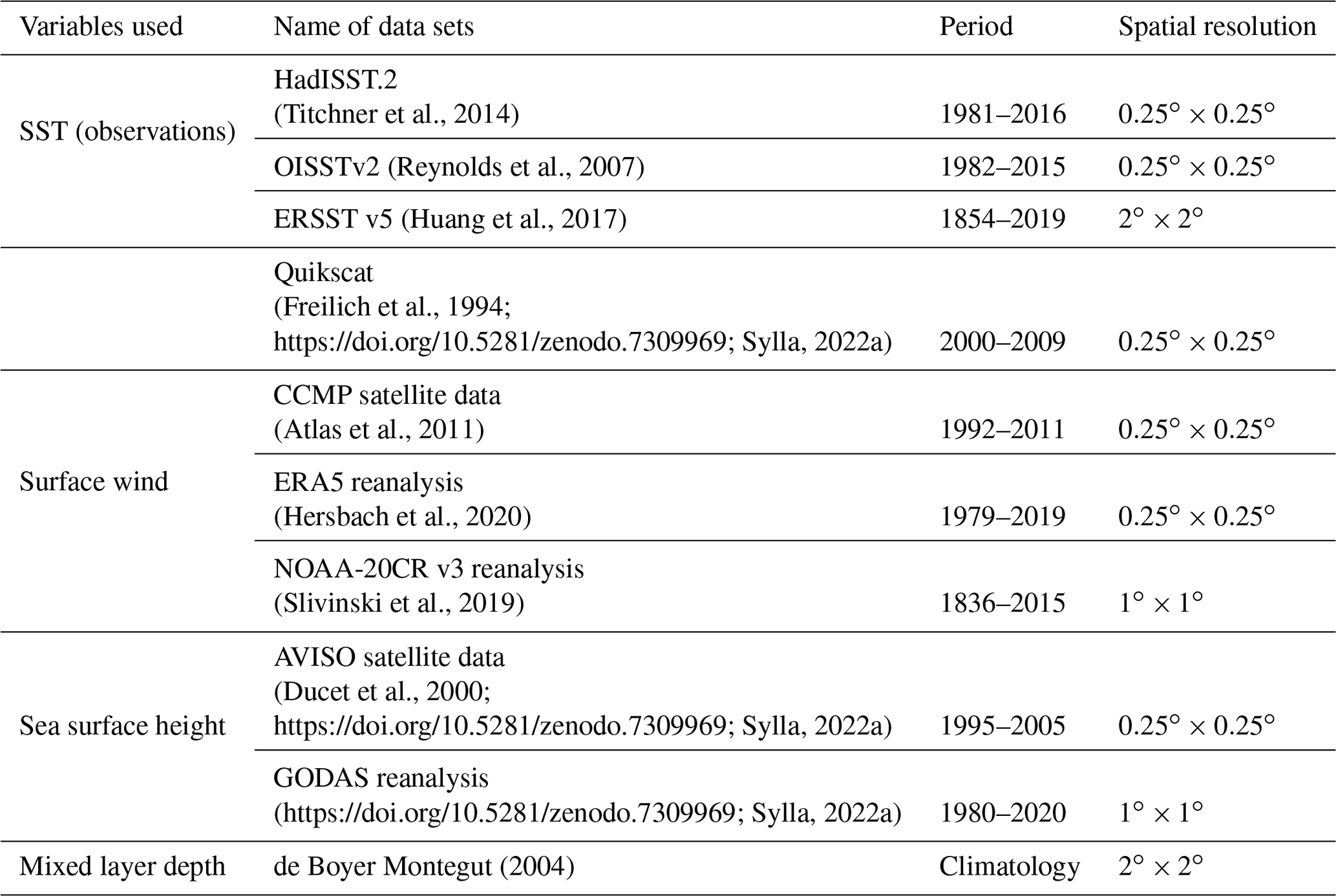
Table 1List of the HighResMIP/PRIMAVERA models used in this study. The first and second columns list the groups and models used. The third and fourth columns indicate the atmosphere and ocean nominal resolution. The last row at the bottom of the table lists the variables that were used for our study: sea surface temperature (SST; called tos in the HighResMIP database), zonal and meridional wind stress components (tauuo and tauvo), sea surface height (SSH; called zos), mixed layer depth (MLD; called mlotst).

2.1 Models and numerical experiments
The coupled models considered in this work are those participating in the European H2020 HighResMIP/PRIMAVERA project (https://www.primavera-h2020.eu, last access: 9 August 2022), which is part of the international HighResMIP exercise. We use the outputs of coupled historical experiments (referred to as “hist-1950”) covering the period 1950–2014. In particular, the models used are HadGEM3 GC3.1 (Williams et al., 2018), CNRM-CM6-1 (Voldoire et al., 2019), CMCC-CM2 (Cherchi et al., 2019), MPI-ESM1 (Gutjahr et al., 2019), ECMWF-IFS (Roberts et al., 2018), and EC-Earth3P (Haarsma et al., 2020). The main characteristics of these models are listed in Table 1 together with the respective effective resolutions in both the atmosphere and ocean components. Note that for the PRIMAVERA coordinated project, resolution was increased in both the atmosphere and the ocean components, with the exception of CMCC-CM2 and MPI-ESM1, in which only the atmospheric resolution was modified. Based on the change in ocean and/or atmosphere resolution four groups of models are defined: groups 1 and 1*, including low-resolution (LR) models, and groups 2 and 2*, including high-resolution (HR) models, for both the atmosphere and the ocean. From group 1 to group 2, both the ocean and the atmosphere resolutions are increased. From group 1* to group 2*, only the atmosphere resolution is increased. Note that our set of models is an ensemble which does not allow a precise comparison of the effect of increasing both ocean and atmosphere resolution on the one hand (groups 1–2) or only increasing the atmosphere resolution on the other hand (1*–2*). Indeed, the resultant model groups do not contain the same models and are not of the same side. Thus, some of the differences among the ensembles of model groups may be due to the intrinsic model biases rather than an effect of model resolution. This drawback has to be kept in mind. Furthermore the terms “standard resolution” and “high resolution” are rather subjective and depend on the context. Here, we use them in the context of global climate modeling so that standard resolution is around 1∘ for the ocean and high-resolution around 0.25∘. We acknowledge that the high-resolution ocean models in this study can barely resolve the first baroclinic Rossby radius deformation (20-60 km; Chelton et al., 1998) in most parts of the CUS. Similarly, the standard atmospheric resolution is 1∘ to 2.5∘, while most of the high-resolution atmospheric components in this study are about 0.5∘, which may not be able to resolve realistic wind structure or drop-off near the coast (Patricola and Chang, 2017). So, even models described here as “high-resolution” can probably realistically not resolve upwelling dynamics in this region, at least not as well as dedicated configurations (for example Regional Ocean Modeling System, ROMS, numerical simulation including a high-resolution (∼2 km) grid and a standard-resolution (∼10 km) grid (e.g, Ndoye et al., 2017).
Sylla, 2022aSylla, 2022aSylla, 2022aTable 2Observations and reanalysis data sets selected for this study and specifications of their resolution and coverage period.
Our analysis is based on the SST wind stress, sea surface height, and mixed layer depth monthly fields (see Sect. 2.3). For each variable we compute the 30-year climatological mean for the period 1985–2014. The choice of this period is motivated by the selection of a common period among the various observational data sets used in this study. To avoid biased multi-model ensemble means, only one member of each model was used even if several members are available for certain models. Note that the different members have been averaged together in order to increase robustness of the seasonal cycle estimation; nevertheless the results do not change (not shown). Additionally, the choice can also be justified by the fact that our metrics are based on climatological averages and not on variance or trend metrics, which are more sensitive to internal climate variability.
2.2 Observational and reanalysis products
Several observational and reanalysis data sets are used in the present analysis (see Table 2 for details) in order to evaluate model results' realism in simulating the CUS. For SST, we use the monthly HadISST.2 data set, which was developed at the Met Office Hadley Centre for Climate Prediction and Research (Titchner and Rayner, 2014) We have also used the version 2 of the National Oceanic and Atmospheric Administration (NOAA) Optimum Interpolation Sea Surface Temperature (OISST-v2) analysis (Reynolds et al., 2007). The OISST analysis combines Advanced Very High Resolution Radiometer (AVHRR) satellite data and buoy- and ship-based observations from the International Comprehensive Ocean Atmosphere Data Set (ICOADS) database (Worley et al., 2005). Although these data are provided at daily frequency, monthly averages have been computed. Finally, we have also included the latest version of the Extended Reconstructed Sea Surface Temperature data set (ERSST-v5; Huang et al., 2017). The monthly ERSST-v5, produced by the NOAA, is based on in situ (ship and buoy) observations from ICOADS.
The Quikscat wind speed and the zonal and meridional components of the 10 m wind from the Cross-Calibrated Multi-Platform (CCMP) project are also analyzed (Freilich and Spencer, 1994; Atlas et al., 2011). In addition to the observational products, near-surface wind data from two atmospheric reanalyses (ERA5 and NOAA-20CR v3) have been considered and compared to the previous observational wind products using a wind rose diagram (Fig. A1 in Appendix A). ERA5 is the latest climate reanalysis, provided by the European Centre for Medium-Range Weather Forecasts (ECMWF; Hersbach et al., 2020). The NOAA-20CR v3 (Slivinski et al., 2019) datasets are supported by the National Oceanic and Atmospheric Administration (NOAA), the Cooperative Institute for Research in Environmental Sciences (CIRES), and the US Department of Energy.
Because of a lack of wind stress observations and reanalysis covering the entire domain and period of our study (1985–2014), the surface wind speed is converted into wind stress following an empirical method (see Appendix A for more details). Note that this offline computation of the wind stress is only performed for the observations and reanalysis wind data sets but not for the model, which directly provides the wind stress field.
Meridional sea surface height (SSH) gradients may also play an important dynamical role in coastal regions through geostrophic transport (Marchesiello and Estrade, 2010). Cross-shore geostrophic transport can substantially alter the vertical transport relative to wind-based estimates (Rossi et al., 2013, and Jacox et al., 2014). Thus including the geostrophic component is also important to assess the realism of the modeled upwelling (Rykaczewski et al., 2015, and Oerder et al., 2015). To evaluate the models' representation of SSH along the CUS, we use the AVISO satellite altimetry product (Ducet et al., 2000). For comparison, we have also used the monthly mean SSH from GODAS. Furthermore, quantifying the effect of the SSH gradient on the geostrophic transport requires an estimation of the oceanic mixed layer depth (MLD). We use the MLD climatology from de Boyer Montégut (2004). This MLD climatology is based on ARGO profiles where MLD was estimated following a density criterion at a monthly resolution. The selected criterion is a threshold value of temperature (namely 0.2 ∘C) from a near-surface value at 10 m depth.
Monthly climatologies over the 1985–2014 period are considered for all the validation data sets and models as specified in Sect. 2.1, except for CCMP and AVISO, which are both based on a shorter time period (1992–2011 and 1995–2005 respectively).
2.3 Upwelling indices
We compute the upwelling indices developed in Sylla et al. (2019) for the SMUS and applied here to the whole CUS. The relevance of these indices to represent CUS variability is justified in Sect. 3. We consider the SST difference between the coast (black dots along the Canary coast, Fig. 1) and the outer ocean (magenta dots, Fig. 1) in such a way that the SST-based index is defined by
Typically a distance of 5∘ longitude from the coast is considered for this index (Cropper et al., 2014, and Sylla et al., 2019). This SST upwelling index has been widely used to characterize upwelling intensity as it measures the impact of upwelling on the SST zonal structure (Mittelstaedt, 1991; Santos et al., 2005; Gómez-Gesteira et al., 2008; Lathuilière et al., 2008; and Marcello et al., 2011). Positive (negative) values of the index correspond to more intense upwelling (downwelling).
As described in the introduction section, the influence of wind on the upwelling can be separated into two mechanisms (Sverdrup et al., 1942; Yoshida, 1995; and Smith, 1968). The first mechanism, called the cross-shore Ekman transport (hereafter CSET), is commonly used for characterizing coastal upwelling (Bakun, 1973; Schwing et al., 1996; and Gómez-Gesteira et al., 2008). CSET is computed as the offshore component of Ekman transport (Q), whose zonal and meridional components are derived from the wind stress field as follows:
where ρw is the seawater density (1025 kg m−3), and f is the Coriolis parameter. Following Santos et al. (2012), the zonal and meridional components of the Ekman transport are used to calculate CSET from a discrete set of points parallel to the shoreline (Fig. 1, black dots):
where CSET is expressed in square meters per second, and ϕ represents the angle between the shoreline and the Equator. Whilst presenting a highly irregular topography, the coastline within the CUS can be broadly approximated to 90∘ over the IP, to 55∘ over the MoUS, and to 90∘ off the SMUS coast relative to the Equator (Alvarez et al., 2008, and Cropper et al., 2014). Positive (negative) values of CSET correspond to upwelling-favorable (upwelling-unfavorable) conditions.
The second mechanism contributing to upwelling is the Ekman pumping (Wek) defined as
where Wek is expressed in square meters per second, and represents the curl of the derived wind stress vector integrated over the longitude range of the IP, nMoUS, sMoUS, and SMUS subregions (different boxes in Fig. 1).
Finally, as highlighted in Sect. 2.2, coastal upwelling may be modulated by the cross-shore geostrophic transport. We quantify this effect along the CUS subregions as follows:
where Tgeo is the vertical transport (in sieverts) due to the zonal current generated from the meridional SSH gradient, and g is the gravity coefficient (g=9.81 m s−2). Tgeo is calculated right next to the coastal boundary, where it can interact with the vertical flux. Thus SSHnorth−SSHsouth is the difference between the northernmost and southernmost grid point close to the shore of the different subregions of the CUS (see Fig. 1). In addition, the MLD is averaged over each box marked in Fig. 1 (IP, nMoUS, sMoUS, and SMUS subregions). Note that all indices described above are calculated over the native model grid. However, the metric used here (see Sect. 2.4) to evaluate the model skill requires an interpolation. For this and only for the skill calculation (Fig. 6) all the models have been interpolated from their native grids to a common lat–long-resolution grid, using a bilinear interpolation method. We noted that small changes are induced by the interpolation method (not shown), but this does not affect the skill scores in a statistically significant way.
2.4 Skill metrics
We use a metric to quantify the skill of the climate models at representing the CUS characteristics through the different upwelling indices. In this study we use the arcsine Mielke score (M) previously used to evaluate the performance of the HighResMIP/PRIMAVERA model (Bador et al., 2020).
This is a nondimensional metric defined by
where mse is the mean square error, X and Y represent model and observed data respectively, V is the spatial variance, and G is the spatial mean. The arcsine Mielke score reaches a maximum possible value of 1000 when mse is equal to 0, whereas a zero score indicates no skill, and it can even be negative in the worst cases, although this rarely occurs. The skill score is computed separately over the different subdomains of the CUS and for the annual climatological averages of each upwelling index. To compute M all the upwelling indices have been interpolated on a common horizontal grid by using a bilinear interpolation method.
In this section, we describe the upwelling indices defined above computed for the observation data sets. These indices are shown in Figs. 2, 3, 4, and 5 for both the data and models, but only the observation panels are described here. The results from the modeling experiments are described in Sect. 4.

Figure 2Latitude–time plot of UIsst upwelling index (∘C) computed as explained in Sect. 2.3. The time axis shows climatological months over the period 1985–2014 for several model configurations and reference data sets (HadISST, OISST v2, and ERSST v5). Models from groups 1, 1*, 2, and 2* respectively (see Sect. 2.1 for the definition of these groups). Positive (negative) values correspond to upwelling (downwelling) conditions. In each panel, the gray line represents the southern boundary of the IP subregion (37–43∘ N). The horizontal blue lines (dashed lines) are positioned at 21 and 25∘ N (26 and 32∘ N) and give the limitation of the sMoUS (nMoUS), and the black line represents the northern boundary of the SMUS subregion (12–20∘ N). The black (gray) contour shows the contour zero (values C). This index is calculated over the model's native grid.
3.1 The thermal upwelling indices
The seasonal variability in the CUS upwelling intensity as described by the UIsst index is shown in Fig. 2 (left panels) in the observations and reanalysis. Over the IP coast, the strongest positive values of UIsst are observed in summertime (July to September), and the index remains positive but weaker (0.5 ∘C) from November to June. This evolution is consistent with the available literature (Nykjær and Van Camp, 1994; Santos et al., 2005; and deCastro et al., 2008b). The ocean–coast gradient (i.e., the UIsst index) ranges from 1 to 4 ∘C from lat 21 to 32∘ N (MoUS), with high values of UIsst through the whole year in the sMoUS and during summertime (July to September) in the nMoUS. The presence of the abovementioned high values of UIsst throughout the year in the sMoUS is consistent with the permanent upwelling conditions described in previous works (Wooster et al., 1976; Barton et al., 1998; and Gómez-Gesteira et al., 2008). Further south, over the SMUS region, UIsst shows a marked seasonality with positive values of UIsst in winter (upwelling season) and negative values of UIsst in summer.
Figure 2 reveals that although the three observational data sets present a similar behavior of UIsst, substantial differences in the amplitude emerge. The largest discrepancies are found in the sMoUS (whole year) and SMUS (winter) where UIsst, values are significantly lower in ERSST-v5 than in the other data sets. In the rest of the CUS subregions (i.e., IP and nMoUS), a stronger observational agreement is found.
3.2 Dynamical upwelling indices
Figure 3 shows the seasonal cycle of CSET for observations and reanalysis (left panels). Along the western coast of the IP, upwelling-favorable conditions (positive values of CSET) are observed during summer. This is coherent with the strengthening and northward displacement of the Azores High, which promotes northerly winds. This marked upwelling season in summer is consistent with the results obtained from the thermal index (UIsst) and with the previous research (Alvarez et al., 2005; Santos et al., 2005; and Gomez-Gesteira et al., 2006). As for UIsst (Fig. 2), negligible or even negative values of CSET are detected along the IP coast during wintertime, indicating the predominance of downwelling conditions.
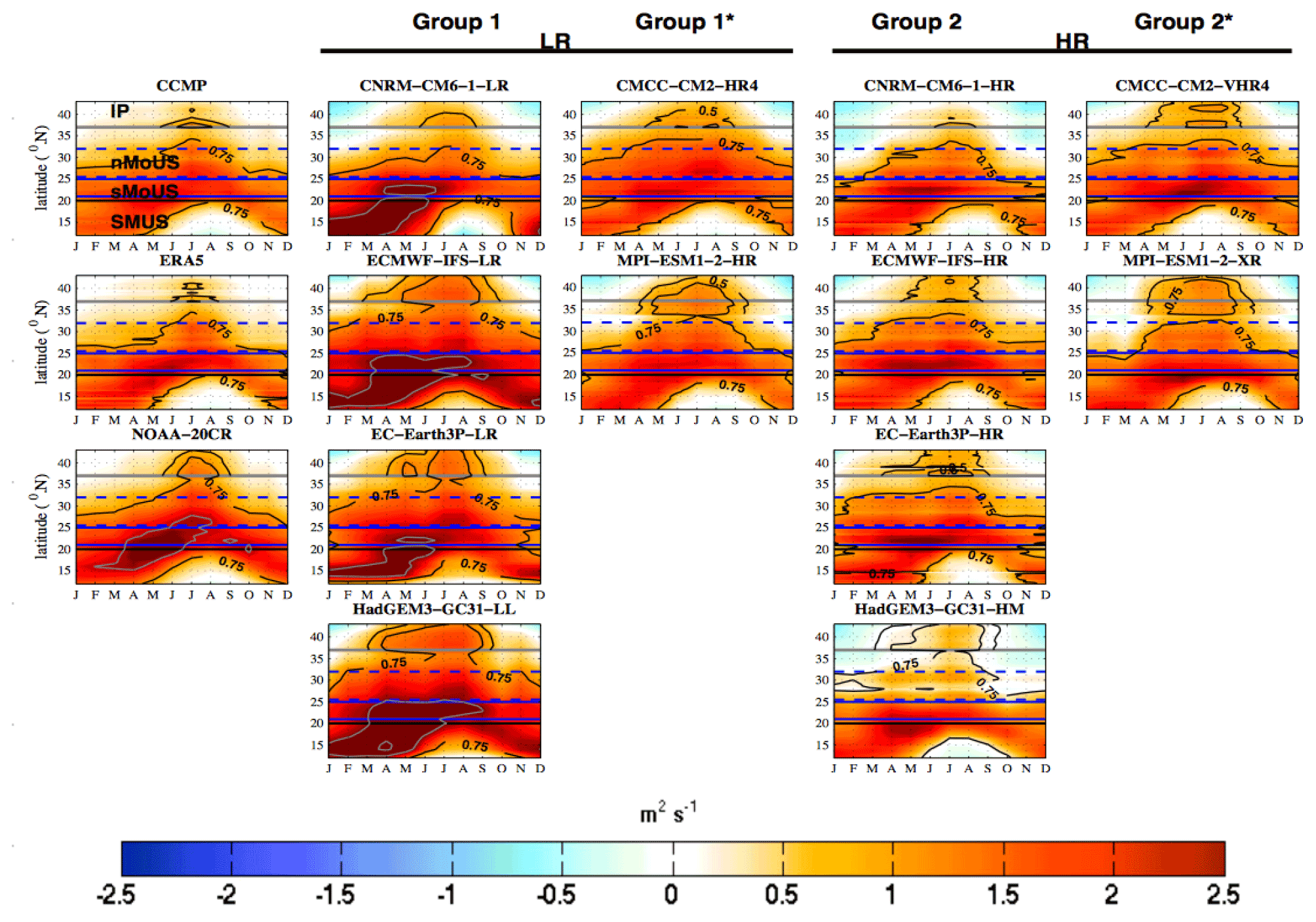
Figure 3Latitude–time plot of CSET upwelling index (m2 s−1) computed over the grid point located along the coast (black stars in Fig. 1). The time axis shows climatological months over the period 1985–2014 (1992–2011) for several model configurations and reference data sets: ERA5 and NOAA-20CR-v3 (CCMP). Models from groups 1, 1*, 2, and 2* respectively (see Sect. 2.1 for the definition of these groups). Positive (negative) values correspond to upwelling (downwelling) conditions. In each panel, the gray line represents the southern boundary of the IP subregion (37–43∘ N). The horizontal blue lines (dashed lines) are positioned at 21 and 25∘ N (26 and 32∘ N) and give the limitation of the sMoUS (nMoUS), and the black line represents the northern boundary of the SMUS subregion (12–20∘ N). The black (gray) contours show the contours 0.5 and 0.75 m2 s−1 (values >2.5 m2 s−1). This index is calculated over the model's native grid
Also consistent with previous studies (Gomez-Gesteira et al., 2006, and Benazzouz et al., 2014), CSET is strong in summer in the nMoUS and permanent throughout the year in the sMoUS. Finally, the SMUS is characterized by the existence of two well-marked seasons: an upwelling season from approximately November to May and a downwelling season from June to October.
As for SST, the comparison between wind products also shows some discrepancies in terms of upwelling amplitude. Despite the CCMP wind data set covering a shorter time period (1992–2011), there is no major difference with respect to ERA5. In contrast, NOAA-20CR-v3 shows a slightly enhanced CSET with respect to the other two data sets, particularly for the SMUS and nMoUS from April to June. A conclusion emerging from this analysis is that the Ekman transport might therefore depend on the underlying size of the grid cell. Thus, gridded data sets at different resolutions may lead to different estimates of the observed Ekman transport. This sensitivity of the Ekman transport to the spatial resolution is therefore crucial to properly compare modeled and observed upwellings.
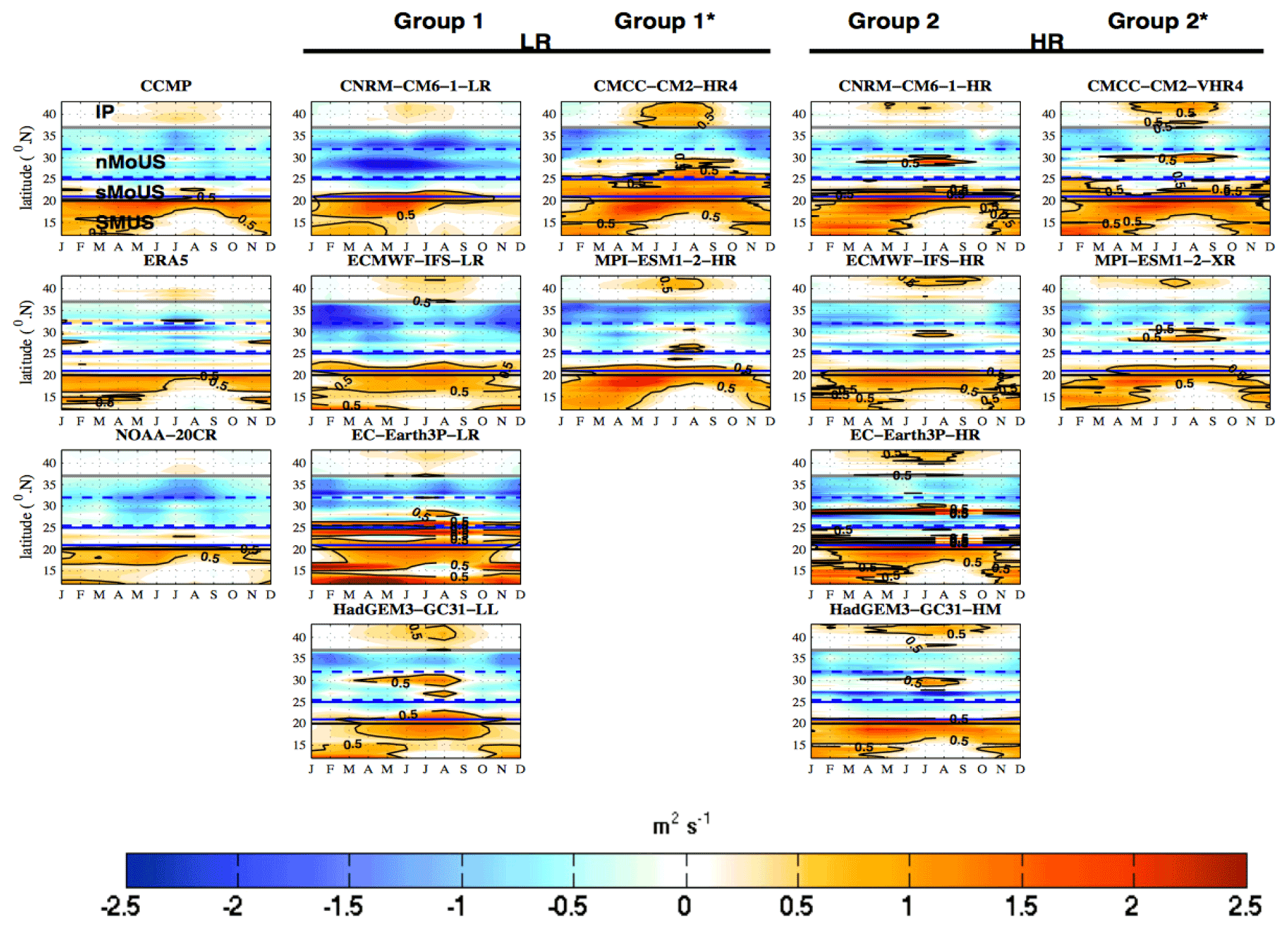
Figure 4Latitude–time plot of integrated Ekman pumping (m2 s−1) calculated as explained in Sect. 2.3. The time axis shows climatological months over the period 1985–2014 (1992–2011) for several model configurations and reference data sets: ERA5 and NOAA-20CR-v3 (CCMP). Models from groups 1, 1*, 2, and 2* respectively (see Sect. 2.1 for the definition of these groups). Positive (negative) values correspond to upwelling (downwelling) conditions. See Fig. 3 for comments on the horizontal lines and contours. This index is calculated over the model's native grid.
Figure 4 shows the seasonal cycle of the Ekman pumping (Wek). Focusing on the validation data sets (left panels) and over the IP, Wek tends to be weak or practically zero from October to June, and it is more intense (around 0.5 m2 s−1) during the summer season in CCMP and ERA5, as found by Alvarez et al. (2008). For NOAA-20CR-v3, this seasonal cycle is less marked. Along the MoUS, Wek is different in the nMoUS and sMoUS subregions. In the sMoUS, Wek is weak but positive, with maximum values occurring during winter and spring. In the nMoUS, validation data sets show mostly negative values of Wek throughout the year, as found by Lathuilière et al. (2008). This result may be linked by the fact that the meridional component of the wind stress (V) decreases (instead of increases) away from the coast. This results in negative in this region (not show) and favorable conditions for downwelling. Finally along the SMUS Wek is maximum in winter and spring. Therefore, the seasonal cycle of Wek is roughly that for CSET (Fig. 3), with the main differences identified over the MoUS.
3.3 The onshore geostrophic flow and the quantitative assessment of the upwelling rate
As discussed in Sect. 2, the effect of Tgeo is quantified here for the CUS. We have firstly examined the monthly climatology of the meridional sea surface height gradient from the AVISO satellite data and the GODAS reanalysis (see first two columns in Fig. B1 of the Appendix B). The SSH gradient observed over the IP (panel a) is indeed negative all year, thus potentially inducing an onshore geostrophic flow. The maximum and minimum amplitudes of this SSH gradient are found in summer and winter respectively. Over the MoUS (panels b and c), this gradient is negative all year as for the IP and reaches its maximum from May to November in the nMoUS and from July to September (August to October) over the sMoUS in AVISO (GODAS). In the SMUS (Fig. B1, panel d) the SSH difference is also always negative, and the related amplitude strongly differs from the other subregions (IP, nMoUS, and sMoUS). Therefore, these SSH meridional gradients yield to an onshore geostrophic transport (Tgeo) off the CUS during the upwelling season. It is important to mention that the latter term (Tgeo) is counted negative eastward following the sign convention used to quantify the upwelling (negative bars in Fig. 5). The Tgeo is below 0.25 Sv over the IP (Fig. 5a) in the three validation data sets. For the nMoUS (Fig. 5b) and sMoUS (Fig. 5c) subregions, Tgeo is on average ∼0.25 Sv. Finally, the contribution of Tgeo is strongest over the SMUS, which presents values of approximately 0.6 Sv. This situation is mainly related to the fact that this subregion shows stronger SSH gradients than the rest of the CUS (panel d, Fig. B1).
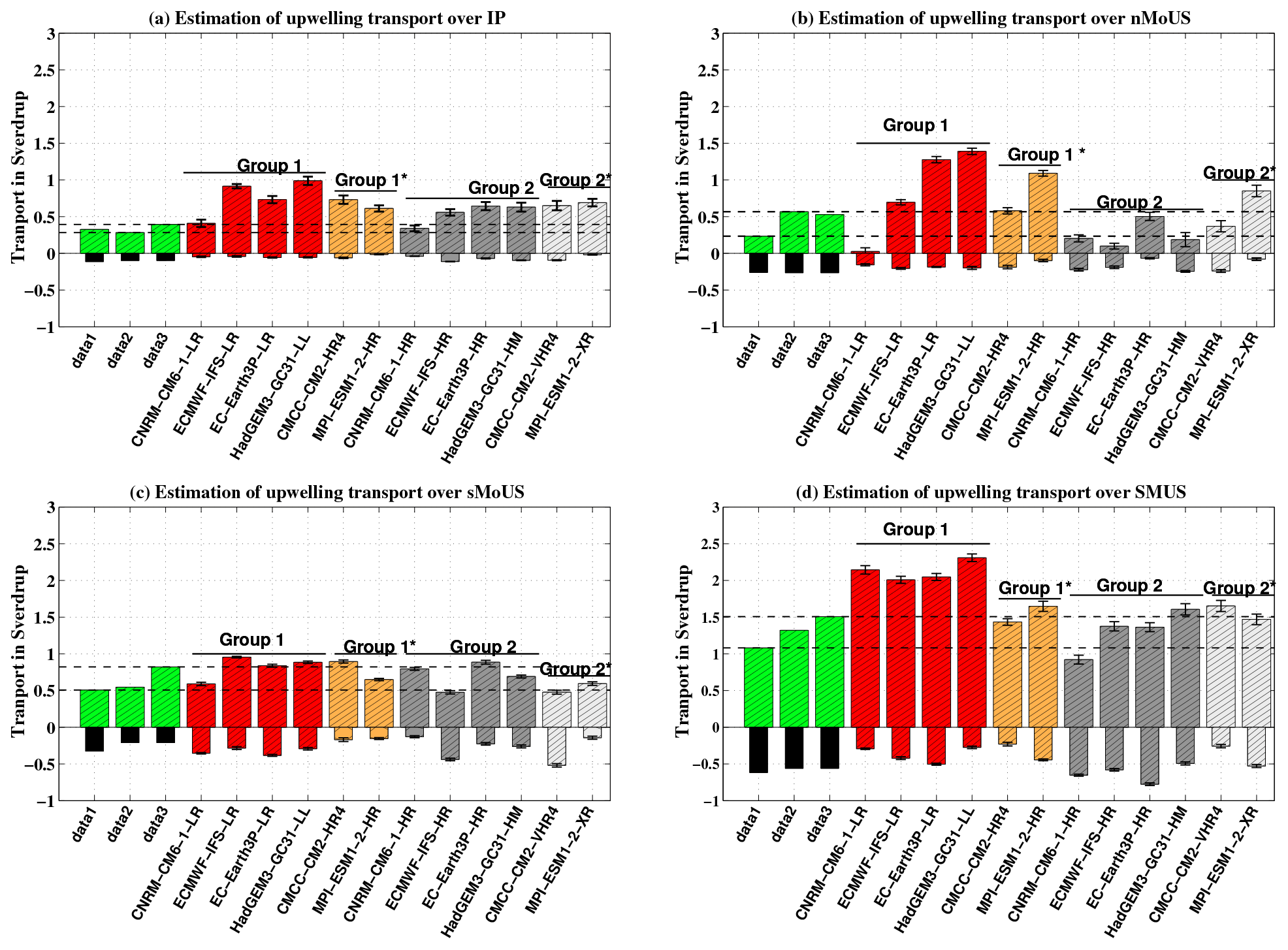
Figure 5Negative bars: estimate of onshore geostrophic flow Tgeo contribution (in Sverdrup; ± error bars: black whiskers bars) computed from Eq. (7) and averaged from July to September over the IP (a) and in the nMoUS (b), all year in the sMoUS (c), and from November to May in the SMUS (d). The first black bar shows Tgeo computed from the AVISO satellite data period (1993–2005) and MLD de Boyer Montégut (2004), and the second and third black bars correspond to Tgeo derived from the GODAS reanalysis (1985–2014) and the previous MLD data. The following columns show the results for the individual climate models. Positive bars show the total volume of upwelling water (UItotal) computed as the sum of the integrated contribution of the three dynamical indices (CSET + Wek + Tgeo) to the upwelling. Data 1 (1993–2005) corresponds to the Ekman process computed from CCMP, Tgeo from the AVISO SSH product, and MLD from de Boyer Montégut (2004). Data 2 and data 3 represent the Ekman process from ERA5 and NOAA-20CR-v3 over 1985–2014 respectively, Tgeo from GODAS, and the same MLD used in data 1. The discontinuous horizontal lines highlighted the observational range.
The physical and biogeochemical responses to coastal divergence and Ekman suction differ in important ways (Capet et al., 2004, and Renault et al., 2016). As a first approach, the CSET and Wek may nevertheless be added up to provide an estimate of upwelling strength. Jacox et al. (2018) have recently suggested that the effect of Ekman processes should be estimated globally from the integration of Ekman transport along the boundaries (north, west, and south) of the region of interest. Comparison of this approach with the one proposed here had been performed with CMIP5 (Sylla et al., 2019). This comparison shows that both methodologies in general yield very similar results. In the validation data sets, the difference is less than 5 %, with the approach of Jacox et al. (2018) leading to slightly stronger results, while the multimodel mean is weakened by approximately 10 %. Given the similarity of these results and the interest, in our view, to discuss the open-ocean wind stress curl separately from the offshore transport divergence, we consider that the overlap is weak and decide to estimate the total upwelling intensity (UItotal) as a sum of the integrated Ekman transport (CSET), the Ekman pumping (Wek), and the geostrophic flow Tgeo.
Furthermore, the comparison of this indirect estimate to a more direct estimate from vertical velocities was also done in Sylla et al. (2019) for CMIP5. The authors show that UItotal is consistent with a direct estimation of the upwelling flux from vertical velocities diagnosed from the models.
Figure 5a (green bars) shows that UItotal over the IP is positive and ranges between 0.25 and 0.45 Sv. UItotal estimation leads to a total upwelling transport of 0.25 to 0.5 Sv over the nMoUS (Fig. 5b), while it ranges from 0.5 to 1 Sv over the sMoUS (Fig. 5c). Note that our previous analysis of Ekman pumping (Fig. 4) has shown negative values during the upwelling season (summer) in the nMoUS favoring the predominance of downwelling conditions. The combination of both Wek and Tgeo may thus contribute to reduce the volume of upwelled waters due to the CSET in this subregion. In the SMUS (Fig. 5d), where the Ekman divergence and the wind stress curl generate a significant vertical transport (Figs. 3 and 4), our estimation of UItotal is about 1 to 1.5 Sv. This upwelling is however partially reduced (as in Sylla et al., 2019) by the strong effect of onshore transport.
4.1 The thermal upwelling indices
To address the model analysis, we compare UIsst from the observational data sets (Fig. 2, left panels) and the different model configurations (Fig. 2, right panels). In the IP, there is a general agreement between observations and models. Models broadly reproduce the climatological seasonal cycle obtained in observations with a maximum in summer. One exception can be noted: the CNRM-CM6 family shows no signature of upwelling with unrealistic negative values of UIsst during summer. In general, the amplitude of the seasonal cycle is slightly enhanced when both the ocean and atmosphere resolutions are increased (comparison among groups 1 and 2).
Along the nMoUS and sMoUS, group 2 provides a more realistic representation of this SST index than their LR versions (group 1). In the latter case the amplitude is markedly underestimated over the sMoUS subregion. For both groups 1* and 2*, the upwelling is broadly reproduced in these subregions, with an overestimation of UIsst amplitude in MPI-ESM1 over the sMoUS. Thus, the only increase in the atmospheric resolution in models produces no clear impact on upwelling representation.
Along the SMUS subregion and for group 1 (i.e., the LR model versions), the upwelling season seems to be longer than that observed: it starts earlier (October) and ends later (June), with a marked drop for CMCC-CM2 (group 1*). However both MPI-ESM1-2-HR and MPI-ESM1-2-XR simulate a realistic seasonal cycle in comparison with the observations, but the corresponding amplitudes are largely overestimated over the sMoUS and the SMUS. This situation may be explained by the results found in Gutjahr et al. (2019). According to these authors the MPI model suffers a severe cold bias in the whole northern hemisphere and, particularly, in the Atlantic sector. In this line, Roberts et al. (2019) show that a higher-resolution atmosphere tends to produce a cooler ocean SST, particularly in the ocean upwelling regions (in agreement with Gent et al., 2010 and Small et al., 2014). This cooling has already been assessed by Putrasahan et al. (2019) and is caused by a slowed Atlantic Meridional Overturning Circulation (AMOC) due to the underestimation of the wind stress, the northward heat, and the salt transport. The abovementioned deficiencies in the representation of the seasonal cycle seem to be improved when both the atmospheric and the ocean resolutions increase (group 2). In contrast, when just the atmospheric resolution is increased they persist (group 2*).
In summary, increasing the horizontal resolution of the atmosphere or both the atmosphere and the ocean alters the representation of the CUS if it is characterized with the thermal index UIsst. Nevertheless, different features are identified along the distinct subregions within the CUS. Thus, the IP does not seem to be very sensitive to these changes in model resolution. In contrast, upwelling representation on the western African coast (MoUS and SMUS) improves when ocean and atmospheric resolutions enhance. This is consistent with Ma et al. (2019) and Balaguru et al. (2021), who found that an increase in horizontal resolution can potentially reduce the warm bias of climate models along these regions through an improved simulation of coastal upwelling. This responds to the fact that the thermocline rises more sharply near the coast, causing a reduction in the near-shore SST bias in the high-resolution global climate models. On the other hand, the comparison of group 1* and group 2* indicates that the upwelling estimated with UIsst does not change significantly when only the atmospheric resolution is increased. Therefore, we infer that enhancing ocean resolution is required to improve the SST-related upwelling index representation over the CUS. This is in agreement with previous studies such as Small et al. (2015) for the Benguela upwelling system. Additionally, Gutjahr et al. (2019) suggest that a high spatial resolution in the ocean reduces the bias in both the ocean interior and the atmosphere. All this leads to the important conclusion that a high-resolution ocean plays a key role for properly representing the ocean and atmosphere mean states.
4.2 Dynamical upwelling indices
As for the thermal index UIsst, we evaluate the ability of the different model configurations to reproduce the seasonal variability in CSET (Fig. 3) and Wek (Fig. 4). Along the IP coast all model configurations show the seasonal variability in CSET with the maximum during summer. However in group 1, the upwelling period is in general overestimated, which is not the case of group 2. Regarding groups 1* and 2*, no major difference has been identified, and it is therefore difficult to extract a relationship with confidence.
Focusing on the sMoUS and nMoUS, group 1 largely overestimates CSET, whereas this overestimation is less clear for group 1* (Fig. 3). In contrast, group 2 is broadly coherent with the observations, and group 2* also provides more realistic CSET values than group 1*. This suggests that higher-resolution winds lead to an improved Ekman transport. Similar conclusions are generally drawn over the SMUS region for groups 1* and 2*, whereas group 2 shows a better agreement with the validation data sets than group 1. The latter again overestimates the amplitude of the Ekman transport with respect to the reference values. This situation has also been documented in Castaño Tierno (2020).
We consider now the ability of the different model configurations to reproduce the seasonal variability in the wind stress curl (Fig. 4). The models reveal sometimes noisy patterns, making the interpretation of the effect of model resolution complex in these cases, but some conclusions can be drawn. Group 2 reproduces the expected larger features of the Wek seasonal cycle in the different subregions, and a comparison with group 1 reveals differences in structure and intensity, particularly over the southern flank (MoUS and SMUS). Group 1 shows generally a rather sharp and unrealistic seasonal cycle in the SMUS, which is longer than that identified in the validation data sets. The improvement in group 2 may be linked to that found by Ma et al. (2019): a finer horizontal resolution of climate models enables better representation of low-level coastal jet structure, with stronger and closer alongshore wind stress and curl leading to a more realistic representation of upwelling. The refinement of just the atmospheric resolution (group 2*) also leads to an improved wind stress curl.
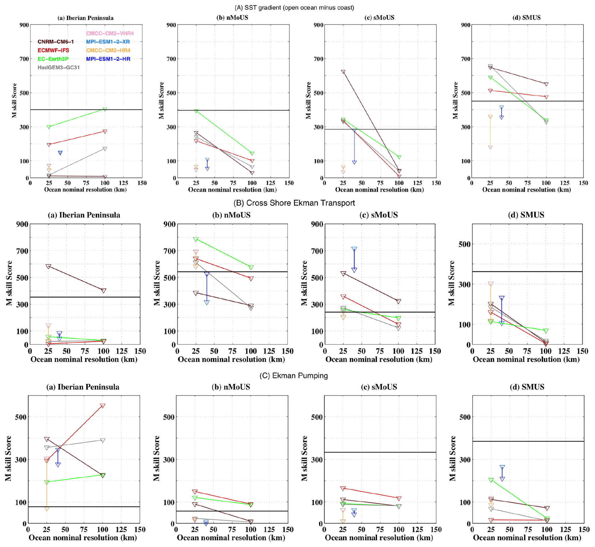
Figure 6M skill score of SST gradient between ocean minus coast (top panels), Ekman transport (central panels), and Ekman pumping (bottom panels) as a function of the ocean model nominal resolution. The models from group 1* and 2* are thus represented by the vertical lines (with their HR version: MPI-ESM1-2-XR and CMCC-CM2-VHR4, highlighted by the light-blue and magenta color respectively). The score is computed and averaged along the IP subregion (a) and the nMoUS (b) from July to September, all year in the sMoUS (c), and from November to May along the SMUS (d) over the period 1985–2014. For the SST index (dynamical indices), each model is evaluated against OISST-v2 (ERA5) observation. The horizontal lines in each panel correspond to the average of the M scores computed from all combinations of pairs of observational products.
4.3 Geostrophic flow and total upwelling transport
Figure 5 shows the total upwelling transport (UItotal) by taking into account the different upwelling terms: CSET, Wek, and Tgeo. The latter (computed as described in Sect. 2.3 and represented in Fig. 5 with negative bars) is too weak in group 1 over the IP coast, which is related to the low contribution of SSH gradient in these models during the upwelling season (Fig. B1 in Appendix B). When both the ocean and atmosphere resolutions are increased (group 2), the realism of Tgeo is improved. It is broadly consistent with the observational estimates. The CMCC-CM2 family in group 1* and 2* provides realistic Tgeo values independently of the model resolution. However, this onshore transport is very low (close to zero) in the MPI-ESM1 models for both resolutions, particularly due to the shallower mixed layer depth (not shown) over the North Atlantic. This feature is consistent with Gutjahr et al. (2019). The effect of increasing only the atmospheric resolution is, therefore, difficult to be established. As in group 1 this is probably due to the relatively weak effect associated with the SSH-related contribution. In the nMoUS and sMoUS (Fig. 5b and c), the role of the resolution in the simulated Tgeo is not clear, and the difference amongst the groups is very small. Finally in the SMUS region, the more realistic estimates of Tgeo are generally provided by group 2 as well as the simulated SSH gradient (Fig. B1). For groups 1* and 2*, the MPI-ESM1 models show better agreement with observations than the CMCC-CM2 models, but the impact of the atmospheric resolution is again not conclusive.
We consider now the total upwelling transport (UItotal) computed as the sum of all dynamical effects, as explained in Sect. 3.2. We find, along the IP coast (Fig. 5a), that both groups 1 and 1* markedly overestimate the upwelling total transport. This overestimation is reduced in group 2, with UItotal values slightly higher than the observational range (horizontal dashed lines). However minor differences are found among groups 1* and 2*.
In the nMoUS, group 1 and group 1* again largely overestimate the total upwelling transport, except for the CNRM-CM6-1-LR, which shows values almost close to zero, and CMCC-CM2-HR4, which provides a generally good estimation of UItotal. The very weak value in CNRM-CM6-1-LR can be explained by the downwelling effect displayed by the Wek, which is relatively strong in this model configuration (Fig. 4). On average, the HR model versions (group 2) perform better than the UItotal, which appears to be within the range of observational estimates. Models of group 2 are generally in the range of observational estimates, and group 2* shows a small improvement with increased resolution. The CMCC-CM2-VHR4 is as close to the validation data sets as its LR version, while MPI-ESM1 always overestimates UItotal, although the value is smaller in the HR version than in the LR version.
In the sMoUS subregion the differences among model resolution are less marked than in the previous regions. Thus, it is difficult to directly relate the representation of UItotal with model resolution. Finally, over the SMUS domain and as seen in Fig. 5d, group 2 has a generally better agreement with the observations than group 1, for which UItotal is clearly outside the range of the observed UItotal. Thus, models in group 2 are able to fully capture the estimation of the upwelling transport by realistically representing all the dynamical indices in such a way that the simulated upwelling in this subregion tends to be systematically more tightly clustered. Groups 1* and 2* show a similar range of UItotal, and no clear effects due to the increasing resolution are identified.
4.4 Quantitative measure of the model skill
In this section, we evaluate quantitatively the performance of the models in simulating the CUS using the arcsine Mielke M score (see Sect. 2.4). M is computed between the observed and the simulated upwelling indices as a function of the nominal ocean resolution. The reference data sets are OISST-v2 for the thermal index (SST-based) and ERA5 for the dynamical (wind-based) indices. Note that the skill score values may be sensitive to the choice of the observational data sets to measure the model performance in some cases (Fig. C1 in Appendix C). For instance, for most subdomains and indices, differences in skill scores computed with HadISST or OISST-v2 (ERA5 for dynamical indices) for UIsst are as large as 250 points between the M skill scores computed with ERSST-v5 (NOAA-20CR-v3), but the slopes of the lines that connect the skill scores at different resolutions remain unchanged. Observational consistency is quantitatively assessed using the average of the M scores computed from each possible combination of pairs of observational data sets. This consistency is represented by the horizontal lines in each panel of Fig. 6. It is moderately high (above 300 points) for the thermal index (top panels) and Ekman transport (central panels) in most of the subregions analyzed. However this value is very low for the Ekman pumping (Fig. 6, bottom panels) in the case of the IP and nMoUS. This feature indicates, for these subdomains, a weaker similarity among the validation data sets. These results illustrate the challenge that exists in providing an accurate characterization of the upwelling systems in observations and reanalysis.
For UIsst (top panels), the slopes of the lines that connect group 1 and group 2 in the MoUS and SMUS (panels b, c, and d) subregions are negative, indicating a higher skill for higher resolution (group 2). However, an opposite behavior is observed over the IP (panel a), where low-resolution models present larger levels of skill. We note no robust change for the M scores between group 1* and group 2*. These results support the conclusions drawn from Fig. 2 in Sect. 4.1. Let us try now to decompose the total Ekman process: for the Ekman transport (Fig. 6, central panels), again the slopes of the lines that connect M values indicate a higher skill for group 2 in the MoUS and SMUS. For group 1* and group 2*, model results are still limited in reaching systematic conclusions on the effect of enhanced resolution in the atmospheric component, although the MPI-ESM1-2-HR clearly shows larger skill score than its LR version in the nMoUS and SMUS subregions. Along the IP subregion, the M scores are not conclusive, except for the CNRM-CM61-HR, which provides a higher score with increased resolution.
Results regarding the Ekman pumping (Fig. 6, bottom panels) are similar to those obtained for the Ekman transport, with improved model performance as both resolutions increase and no systematic response when only the atmospheric grid resolution is modified. However, M values are broadly lower for the Ekman pumping than for the Ekman transport, indicating that models are less efficient in capturing the Ekman pumping than the transport along the coast. The conclusions obtained from the M scores corroborate the results found in the previous section for the individual upwelling indices.
To summarize, increasing both the ocean and atmosphere resolution yields a higher skill score than group 1 in the Morocco and SMUS upwelling systems, but no significant improvement in simulating the Iberian Peninsula upwelling system is found. On the other hand, within the investigated range, increasing atmosphere resolution has a limited effect on the skill scores. Nevertheless, it is necessary to note that only two models form group 2*, which makes it difficult to extract a significant relationship between increased atmosphere resolution and model performance.
This study provides the first attempt to systematically evaluate the effect of increasing global model resolution (in both the atmosphere and ocean components) on the representation of the CUS. We have analyzed the historical simulations from six global climate models following the HighResMIP protocol (Haarsma et al., 2016). Four upwelling indices based on SSTs, wind stress, and sea surface height have been used as metrics to assess the effects of increased model resolution. A quantitative skill metric, the arcsine mean skill score, has also been applied to measure the models' performance with respect to observational data sets. The most relevant findings can be summarized as follows.
Globally, our results show that observations and reanalysis yield a fairly consistent picture of the CUS climatology. However in the southern part of Morocco and in the Senegalo–Mauritanian areas, upwelling indices derived from the validation data sets at lower resolution (ERSST-v5 and NOAA-20CR-v3) show greater magnitudes than those derived from the higher-resolution data sets. The average of the M skill scores used to quantify the consistency among observational and reanalysis data sets at different resolutions is not very high. This highlights the challenge that exists for choosing a proper observational data set to evaluate global climate models' performance.
The impact of increasing model resolution is not the same in the different subdomains of the CUS. In the northern part, within the IP domain, the high-resolution models do not seem to better simulate the structure of the climatological SSTs and the winds linked to the upwelling. For some models the LR version even produces better results than the HR version. However, in the southern CUS, and in particular in the MoUS and SMUS, the HR models show a clear improvement in the representation of upwelling indices. Increasing the resolution leads to simulations that are in better agreement with the observations. The best results are obtained when the resolution is increased for both components of the coupled models, ocean and atmosphere. According to our results, the effect of increasing only the atmospheric resolution is not clear. This is probably mainly due to the fact that the sample analyzed in this case is small (only two models). The results presented here suggest nevertheless that increasing the resolution of the atmospheric component is not enough and that it is also necessary to increase the resolution of the ocean to obtain a significant improvement in the representation of the CUS. The oceanic resolution emerges therefore as a key factor for having more realistic simulations, which is in agreement with other studies (e.g., Bryan et al., 2010; Putrasahan et al., 2013; Parfitt et al., 2017 and Bellucci et al., 2021). Our results are also in line with previous modeling work suggesting that an increased resolution improves global climate model performance. Roberts et al. (2019) have shown that increased model resolution in the atmosphere and ocean can have a considerable impact on the large tropical Atlantic biases seen in typical CMIP-resolution models of the mean state and variability, both at the surface in terms of temperature and in the deeper ocean. According to Czaja et al. (2019), a clear dependence on resolution (both ocean and atmosphere) is found, and there is better agreement with reanalysis and observations. However, this issue may also be model- and region-dependent (Delworth et al., 2012, and Raj et al., 2019). In the present study, the representation of oceanic processes related to upwelling has not been investigated in detail. Further work is needed to better understand the role of the ocean dynamic on the simulated upwelling improvements, in particular for comparing groups 1 and 2. The effect of stratification in particular is not investigated in this study. Comparing ocean stratification and vertical transport between groups 1 and 2 can indeed provide insight into the relative role of increased ocean and atmospheric resolution in improving the representation of upwelling.
This study provides encouraging results for high-resolution global climate modeling, although many aspects related to the physical processes must be further assessed in the future. However, as already argued in previous studies that have analyzed HighResMIP simulations (Bador et al., 2020; Moreno-Chamarro et al., 2022; and López-Parages and Terray, 2022), increasing the resolution of a global climate model does not necessarily have to be the only way to better represent the climate system. There is still much work to be done in terms of physical parameterizations as suggested by Patricola et al. (2012) and Harlaß et al. (2018). The improvements in model parametrizations and process representations, specific corrections applied to models, additional tuning, and longer spin-ups might all be essential. On the other hand, climate variability is particularly important in the near term and for highly variable quantities such as precipitation. But this might not be the case of coastal upwelling. Indeed, individual members of high-resolution models show no difference when simulating the Canary upwelling system (not shown). We might infer that individual model runs do not necessarily represent independent estimates, and therefore, it may be more convenient to only run a small subset of ensemble members for models at high resolution (although computationally expensive) than a large subset of ensemble members for models at standard resolution. This and other related questions must be necessarily faced in future works.
We compare the wind data sets used in this study by performing an analysis of the wind roses over the CUS region (Fig. A1). To simplify the data set comparison, we consider 1 month (August for the IP and MoUS and February for the SMUS) when upwelling occurs in these subregions. Along the Iberian Peninsula coast (first column) and over the Morocco (second column) to the Senegalese–Mauritanian coast (last column) the trade winds blow from the northwest to northeast approximately 10 % to 35 % and 15 % to 60 % of the selected time at speeds ranging between 2.5 and 5 m s−1 and between 5 and 10 m s−1 respectively. We note a good similarity among wind data sets, across all the considered domains. Quikscat slightly overestimates the wind speed over the SMUS. Therefore, we chose to work with CCMP because it covers a larger period of time than Quikscat. Additionally the agreement between ERA5 and NOAA-20CR-v3 with the observations provides good support for using these reanalyses, exactly matching the present period considered in the climate models (1985–2014).
For all validation data, the wind stress was computed using the bulk formula as Santos et al. (2012) and Sylla et al. (2019):
where uas and vas are the zonal and meridional wind components respectively, Cd the drag coefficient (Cd=0.0014), and ρa the air density (ρa=1.22 kg m−3).
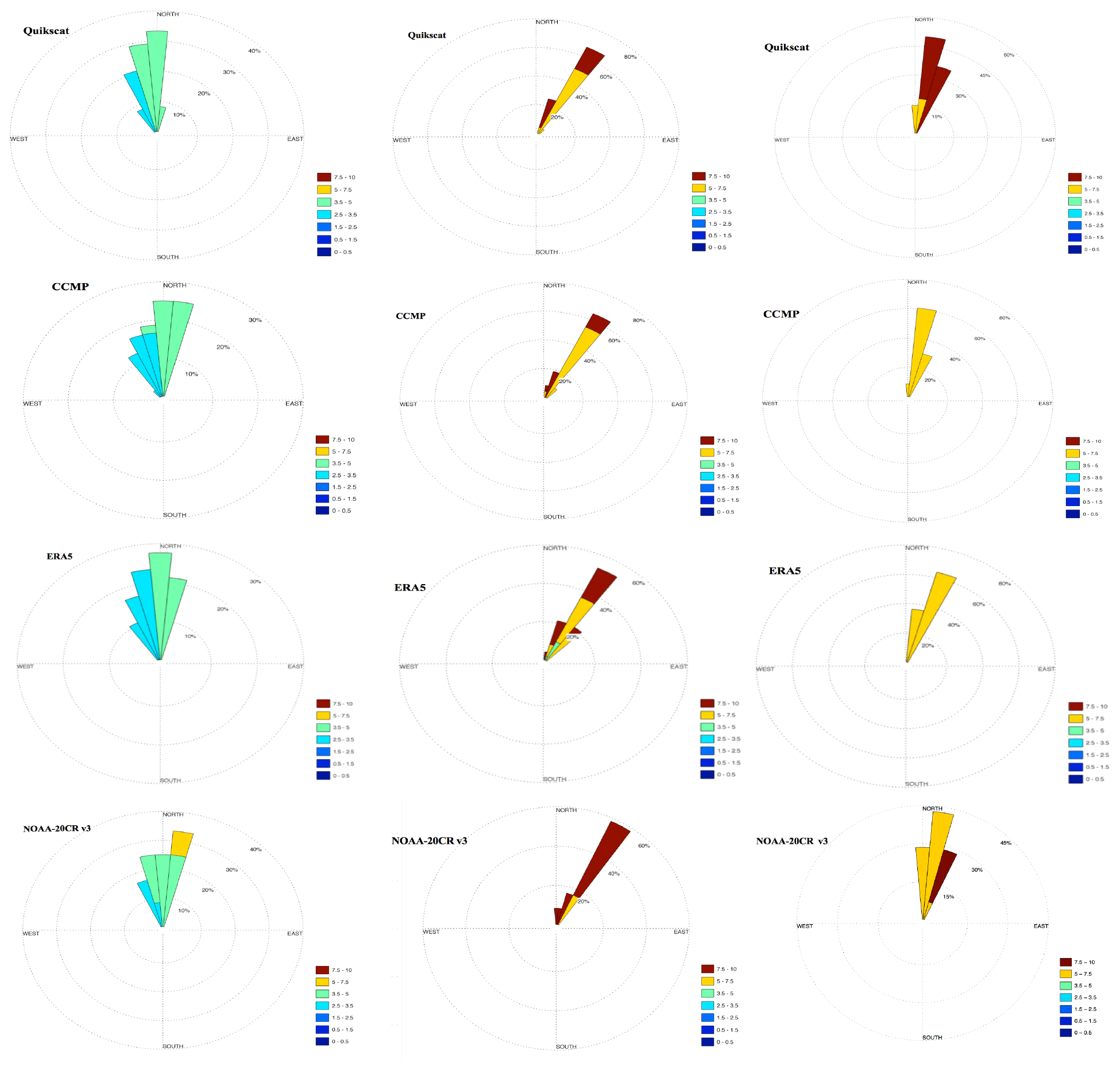
Figure A1Wind rose diagram in August and averaged over the period 2000–2009 along the Iberian Peninsula (first column) and Morocco (second column) subregions and in February along the Senegalo–Mauritanian subregion (last column) from the Quikscat, CCMP, ERA5, and NOAA-20CR-v3 wind products. The concentric circles represent a different frequency range, ranging from zero at the center to increasing frequencies at the outer circles. The different colors provide information on the wind speed (m s−1) for each direction.
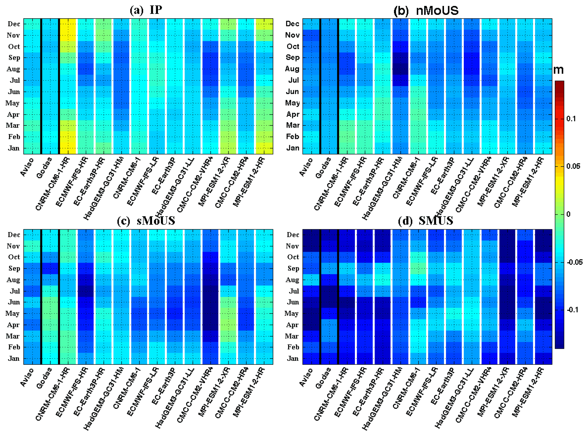
Figure B1Monthly climatology of the meridional sea surface height difference (units: meters) between coastal SSH values at the northernmost and southernmost grid point close to the shore over the Iberian Peninsula (a) and northern and southern Morocco subdomains (panels b and c respectively) and in the Senegalo–Mauritanian subregion (panel d). The first two columns on the left (highlighted in black) show the results from AVISO satellite data (1993–2005) and GODAS reanalysis (1985–2014) respectively. The other bands show the individual HighResMIP models.

Figure C1M skill score of upwelling indices as Fig. 6, with each model evaluated against the SSTs data sets (OISST-v2, HadISST, and ERSST-v5) for the thermal index and to ERA5 and NOAA-20CR-v3 for the dynamical indices.
All of the HighResMIP/PRIMAVERA model outputs analyzed in this paper for HadGEM3 GC3.1 (Williams et al., 2018), CNRM-CM6-1 (Voldoire et al., 2019), CMCC-CM2 (Cherchi et al., 2019), MPI-ESM1 (Gutjahr et al., 2019), ECMWFIFS (Roberts et al., 2019), and EC-Earth3P (Haarsma et al., 2020) are openly accessed through the Earth System Grid Federation (ESGF) nodes. The datasets (observations and reanalyses) supporting the conclusions of this article are available in the Zenodo archive (https://doi.org/10.5281/zenodo.7309969; Sylla, 2022a). The code developed for the core computations of this study can be found under https://doi.org/10.5281/zenodo.7309780 (Sylla, 2022b).
AS is the first author of the paper and performed the largest part of the analysis. ESG, JM, and JLP contributed with ideas and writing and approved the submitted version.
The contact author has declared that none of the authors has any competing interests.
Publisher’s note: Copernicus Publications remains neutral with regard to jurisdictional claims in published maps and institutional affiliations.
This work is carried out as part of the TRIATLAS project (Tropical and South Atlantic climate-based marine ecosystem predictions for sustainable management). The authors thank the colleagues within the climate group of CERFACS (https://cerfacs.fr/en/climate-variability-and-predictability/, last access: 12 September 2022) for their interesting discussions and feedback.
This work was mainly funded by European Union Horizon (H2020) research and innovation program (grant no. 817578), as part of the TRIATLAS project.
This paper was edited by Riccardo Farneti and reviewed by three anonymous referees.
Alvarez, I., deCastro, M., Gomez-Gesteira, M., and Prego, R.: Inter-and intra-annual analysis of the salinity and temperature evolution in the Galician Rias Baixas-ocean boundary (northwest Spain), J. Geophys. Res., 110, C04008, https://doi.org/10.1029/2004JC002504, 2005. a, b
Alvarez, I., Gomez-Gesteira, M., deCastro, M., and Dias, J. M.: Spatiotemporal evolution of upwelling regime along the western coast of the Iberian Peninsula, J. Geophys. Res., 113, C07020, https://doi.org/10.1029/2008jc004744, 2008. a, b, c
Arístegui, J., Barton, E. D., Tett, P., Montero, M. F., García-Muñoz, M., Basterretxea, G., Cussatlegras, A.-S., Ojeda, A., and de Armas, D.: Variability in plankton community structure, metabolism, and vertical carbon fluxes along an upwelling filament (Cape Juby, NW Africa), Prog. Oceanogr., 62, 95–113, https://doi.org/10.1016/j.pocean.2004.07.004, 2004. a
Arístegui, J., Barton, E. D., Álvarez-Salgado, X. A., Santos, A. M. P., Figueiras, F. G., Kifani, S., Hernández-León, S., Mason, E., Machú, E., and Demarcq, H.: Sub-regional ecosystem variability in the Canary Current upwelling, Prog. Oceanogr., 83, 33–48, https://doi.org/10.1016/j.pocean.2009.07.031, 2009. a, b, c
Atlas, R., Hoffman, R. N., Ardizzone, J., Leidner, S. M., Jusem, J. C., Smith, D. K., and Gombos, D.: A Cross-calibrated, Multiplatform Ocean Surface Wind Velocity Product for Meteorological and Oceanographic Applications, B. Am. Meteorol. Soc., 92, 157–174, https://doi.org/10.1175/2010bams2946.1, 2011. a
Bador, M., Boe, J., Terray, L., Alexander, L., Baker, A., Koenigk, T., Putrasahan, D., Roberts, M., Scoccimarro, E., Schiemann, R., Seddon, J., Senan, R., and Valcke, S.: Impact of higher spatial atmospheric resolution on precipitation extremes over land in global climate models, J. Geophys. Res., 125, e2019JD032184, https://doi.org/10.1029/2019JD032184, 2020. a, b
Bakun, A.: Coastal upwelling indices, west coast of North America, 1946–71, U.S. Dep. Commer., NOAA Tech. Rep. NMFS SSRF-671, 103 pp., 1973. a
Bakun, A.: Coastal Ocean Upwelling, Science, 247, 198–201, https://doi.org/10.1126/science.247.4939.198, 1990. a, b
Bakun, A. and Nelson, C. S.: The Seasonal Cycle of Wind-Stress Curl in Subtropical Eastern Boundary Current Regions, J. Phys. Oceanogr., 21, 1815–1834, https://doi.org/10.1175/1520-0485(1991)021<1815:tscows>2.0.co;2, 1991. a
Balaguru, K., Van Roekel, L. P., Leung, L. R., and Veneziani, M.: Subtropical Eastern North Pacific SST bias in earth system models, J. Geophys. Res.-Oceans, 126, e2021JC017359, https://doi.org/10.1029/2021JC017359, 2021. a
Barton, E.D, Arístegui, J., Tett, P., Cantón, M., García-Braun, J., Hernández-León, S., Nykjaer, L., Almeida, C., Almunia, J., Ballesteros, S., Basterretxea, G., Escánez, J., Garcı́a-Weill, L., Hernández-Guerra, A., López-Laatzen, F., Molina, R., Montero, M.F., Navarro-Pérez, E., Rodrı́guez, J.M., Van Lenning, K., Vélez, H., and Wild, K.: The transition zone of the Canary current upwelling region, Prog. Oceanogr., 41, 455–504, 1998. a
Barton, E., Field, D., and Roy, C.: Canary current upwelling: More or less?, Prog. Oceanogr., 116, 167–178, https://doi.org/10.1016/j.pocean.2013.07.007, 2013. a
Bellucci, A., Athanasiadis, P. J., Scoccimarro, E., Ruggieri, P., Gualdi, S., Fedele, G., Haarsma, R. J., Garcia-Serrano, J., Castrillo, M., Putrahasan, D., Sanchez-Gomez, E., Moine, M.-P., Roberts, C. D., Roberts, M. J., Seddon, J., and Vidale, P. L.: Air-Sea interaction over the Gulf Stream in an ensemble of HighResMIP present climate simulations, Clim. Dynam., 56, 2093–2111, https://doi.org/10.1007/s00382-020-05573-z, 2021. a
Benazzouz, A., Mordane, S., Orbi, A., Chagdali, M., Hilmi, K., Atillah, A., Lluís Pelegrí, J., and Hervé, D.: An improved coastal upwelling index from sea surface temperature using satellite-based approach – The case of the Canary Current upwelling system, Cont. Shelf Res., 81, 38–54, https://doi.org/10.1016/j.csr.2014.03.012, 2014. a, b
Blanton, J. O., Atkinson, L. P., Castillejo, F., and Montero, A. L.: Coastal upwelling of the Rias Bajas, Galicia, northwest Spain, I; hydrographic studies, Rapp. P. V. Reun. Cons. Int. Explor. Mer., 183, 179–190, 1984. a
Blanton, J. O., Tenore, K. R., Castillejo, F., Atkinson, L. P., Schwing, F. B., and Lavin, A.: The relationship of upwelling to mussel production in the rias on the western coast of Spain, J. Mar. Res., 45, 497–511, https://doi.org/10.1357/002224087788401115, 1987. a
Bravo, L., Ramos, M., Astudillo, O., Dewitte, B., and Goubanova, K.: Seasonal variability of the Ekman transport and pumping in the upwelling system off central-northern Chile (∼ 30∘ S) based on a high-resolution atmospheric regional model (WRF), Ocean Sci., 12, 1049–1065, https://doi.org/10.5194/os-12-1049-2016, 2016. a
Bryan, F. O., Tomas, R., Dennis, J. M., Chelton, D. B., Loeb, N. G., and McClean, J. L.: Frontal Scale Air–Sea Interaction in High-Resolution Coupled Climate Models, J. Climate, 23, 6277–6291, https://doi.org/10.1175/2010jcli3665.1, 2010. a
Capet, X. J., Marchesiello, P., and McWilliams, J. C.: Upwelling response to coastal wind profiles, Geophys. Res. Lett., 31, L13311, https://doi.org/10.1029/2004gl020123, 2004. a, b
Cardone, V. J., Greenwood, J. G., and Cane, M. A.: On trends in historical marine wind data, J. Clim., 3, 113–127, 1990. a
Castaño Tierno, A.: Tropical ocean-atmosphere interactions in coupled models, The case of of the Equatorial thermocline and the northwest African upwelling, PhD thesis, https://core.ac.uk/download/pdf/288477594.pdf (last access: 12 July 2022), 2020. a
Cherchi, A., Fogli, P. G., Lovato, T., Peano, D., Iovino, D., Gualdi, S., Masina, S., Scoccimarro, E., Materia, S., Bellucci, A., and Navarra, A.: Global Mean Climate and Main Patterns of Variability in the CMCC-CM2 Coupled Model, J. Adv. Model. Earth Sy., 11, 185–209, https://doi.org/10.1029/2018MS001369, 2019. a
Cropper, T. E., Hanna, E., and Bigg, G. R.: Spatial and temporal seasonal trends in coastal upwelling off Northwest Africa, 1981–2012, Deep-Sea Res. Pt. I, 86, 94–111, https://doi.org/10.1016/j.dsr.2014.01.007, 2014. a, b
Czaja, A., Frankignoul, C., Minobe, S., and Vannière, B.: Simulating the midlatitude atmospheric circulation: what might we gain from high-resolution modeling of air-sea interactions?, Current Climate Change reports, 5, 390–406, 2019. a
Davey, M., Huddleston, M., Sperber, K., Braconnot, P., Bryan, F., Chen, D., Colman, R., Cooper, C., Cubasch, U., Delecluse, P., DeWitt, D., Fairhead, L., Flato, G., Gordon, C., Hogan, T., Ji, M., Kimoto, M., Kitoh, A., Knutson, T., Latif, M., Treut, H. L., Li, T., Manabe, S., Mechoso, C., Power, S., Roeckner, E., Terray, L., Vintzileos, A., Voss, R., Wang, B., Washington, W., Yoshikawa, I., Yu, J., Yukimoto, S., Zebiak, S., and Meehl, G.: STOIC: a study of coupled model climatology and variability in tropical ocean regions, Clim. Dynam., 18, 403–420, https://doi.org/10.1007/s00382-001-0188-6, 2002. a
de Boyer Montégut, C.: Mixed layer depth over the global ocean: An examination of profile data and a profile-based climatology, J. Geophys. Res., 109, C12003, https://doi.org/10.1029/2004jc002378, 2004. a, b, c
deCastro, M., Gomez-Gesteira, M., Alvarez, I., Cabanas, J. M., and Prego, R.: Characterization of fall-winter upwelling recurrence along the Galician western coast (NW Spain) from 2000 to 2005: Dependence on atmospheric forcing, J. Mar. Syst., 72, 145–158, https://doi.org/10.1016/j.jmarsys.2007.04.005, 2008a. a
deCastro, M., Gómez-Gesteira, M., Lorenzo, M., Alvarez, I., and Crespo, A.: Influence of atmospheric modes on coastal upwelling along the western coast of the Iberian Peninsula, 1985 to 2005, Clim. Res., 36, 169–179, https://doi.org/10.3354/cr00742, 2008b. a
Delworth, T. L., Rosati, A., Anderson, W., Adcroft, A. J., Balaji, V., Benson, R., Dixon, K., Griffies, S. M., Lee, H.-C., Pacanowski, R. C., Vecchi, G. A., Wittenberg, A. T., Zeng, F., and Zhang, R.: Simulated Climate and Climate Change in the GFDL CM2.5 High-Resolution Coupled Climate Model, J. Climate, 25, 2755–2781, https://doi.org/10.1175/jcli-d-11-00316.1, 2012. a
Doi, T., Vecchi, G. A., Rosati, A. J., and Delworth, T. L.: Biases in the Atlantic ITCZ in seasonal–interannual variations for a coarse-and a high-resolution coupled climate model, J. Climate, 25, 5494–5511, 2012. a
Ducet, N., Le Traon, P. Y., and Reverdin, G.: Global high-resolution mapping of ocean circulation from TOPEX/Poseidon and ERS-1 and -2, J. Geophys. Res.-Oceans, 105, 19477–19498, https://doi.org/10.1029/2000jc900063, 2000. a
Exarchou, E., Prodhomme, C., Brodeau, L., Guemas, V., and Doblas-Reyes, F.: Origin of the warm eastern tropical Atlantic SST bias in a climate model, Clim. Dynam., 51, 1819–1840, 2018. a
Faye, S., Lazar, A., Sow, B. A., and Gaye, A. T.: A model study of the seasonality of sea surface temperature and circulation in the Atlantic North-eastern Tropical Upwelling System, Frontiers in Physics, 3, 1–20, https://doi.org/10.3389/fphy.2015.00076, 2015. a
Fraga, F.: Upwelling off the Galician Coast, Northwest Spain, in: Coastal Upwelling, Coastal Estuarine, Stud., vol. 1, edited by: Richards, F. A., 176–182, AGU, Washington, D. C., 1981. a
Freilich, M. H., Long, D. G., and Spencer, M. W.: SeaWinds: A scanning scatterometer for ADEOS II – Science overview, Proc. Int. Geoscience and Remote Sensing Symp., Pasadena, CA, IEEE, 960–963, 1994. a
Gent, P. R., Yeager, S. G., Neale, R. B., Levis, S., and Bailey, D. A.: Improvements in a half degree atmosphere/land version of the CCSM, Clim. Dynam., 34, 819–833, 2010. a, b, c
Gomez-Gesteira, M., Moreira, C., Alvarez, I., and deCastro, M.: Ekman transport along the Galician coast (northwest Spain) calculated from forecasted winds, J. Geophys. Res., 111, C10005, https://doi.org/10.1029/2005jc003331, 2006. a, b, c
Gómez-Gesteira, M., de Castro, M., Álvarez, I., Lorenzo, M. N., Gesteira, J. L. G., and Crespo, A. J. C.: Spatio-temporal Upwelling Trends along the Canary Upwelling System (1967–2006), Ann. NY Acad. Sci., 1146, 320–337, https://doi.org/10.1196/annals.1446.004, 2008. a, b, c, d, e, f
Gutjahr, O., Putrasahan, D., Lohmann, K., Jungclaus, J. H., von Storch, J.-S., Brüggemann, N., Haak, H., and Stössel, A.: Max Planck Institute Earth System Model (MPI-ESM1.2) for the High-Resolution Model Intercomparison Project (HighResMIP), Geosci. Model Dev., 12, 3241–3281, https://doi.org/10.5194/gmd-12-3241-2019, 2019. a, b, c, d, e
Haarsma, R., Acosta, M., Bakhshi, R., Bretonnière, P.-A., Caron, L.-P., Castrillo, M., Corti, S., Davini, P., Exarchou, E., Fabiano, F., Fladrich, U., Fuentes Franco, R., García-Serrano, J., von Hardenberg, J., Koenigk, T., Levine, X., Meccia, V. L., van Noije, T., van den Oord, G., Palmeiro, F. M., Rodrigo, M., Ruprich-Robert, Y., Le Sager, P., Tourigny, E., Wang, S., van Weele, M., and Wyser, K.: HighResMIP versions of EC-Earth: EC-Earth3P and EC-Earth3P-HR – description, model computational performance and basic validation, Geosci. Model Dev., 13, 3507–3527, https://doi.org/10.5194/gmd-13-3507-2020, 2020. a, b
Haarsma, R. J., Roberts, M. J., Vidale, P. L., Senior, C. A., Bellucci, A., Bao, Q., Chang, P., Corti, S., Fučkar, N. S., Guemas, V., von Hardenberg, J., Hazeleger, W., Kodama, C., Koenigk, T., Leung, L. R., Lu, J., Luo, J.-J., Mao, J., Mizielinski, M. S., Mizuta, R., Nobre, P., Satoh, M., Scoccimarro, E., Semmler, T., Small, J., and von Storch, J.-S.: High Resolution Model Intercomparison Project (HighResMIP v1.0) for CMIP6, Geosci. Model Dev., 9, 4185–4208, https://doi.org/10.5194/gmd-9-4185-2016, 2016. a, b, c
Harlass, J., Latif, M., and Park, W.: Improving climate model simulation of tropical Atlantic sea surface temperature: The importance of enhanced vertical atmosphere model resolution, Geophys. Res. Lett., 42, 2401–2408, 2015. a
Harlaß, J., Latif, M., and Park, W.: Alleviating tropical Atlantic sector biases in the Kiel climate model by enhancing horizontal and vertical atmosphere model resolution: climatology and interannual variability, Clim. Dynam., 50, 2605–2635, https://doi.org/10.1007/s00382-017-3760-4, 2018. a
Herbland, A. and Voituriez, B.: La production primaire dans l'upwelling mauritanien en mars 1973, Cah. O.R.ST.OM., Sér. Océanogr., 12, 187–201, 1974. a
Hersbach, H., Bell, B., Berrisford, P., Hirahara, S., Horányi, A., Muñoz-Sabater, J., Nicolas, J., Peubey, C., Radu, R., Schepers, D., Simmons, A., Soci, C., Abdalla, S., Abellan, X., Balsamo, G., Bechtold, P., Biavati, G., Bidlot, J., Bonavita, M., Chiara, G., Dahlgren, P., Dee, D., Diamantakis, M., Dragani, R., Flemming, J., Forbes, R., Fuentes, M., Geer, A., Haimberger, L., Healy, S., Hogan, R. J., Hólm, E., Janisková, M., Keeley, S., Laloyaux, P., Lopez, P., Lupu, C., Radnoti, G., Rosnay, P., Rozum, I., Vamborg, F., Villaume, S., and Thépaut, J. N.: The ERA5 global reanalysis, Q. J. Roy. Meteor. Soc., 146, 1999–2049, https://doi.org/10.1002/qj.3803, 2020. a
Hewitt, H. T., Roberts, M., Mathiot, P., Biastoch, A., Blockley, E., Chassignet, E. P., Fox-Kemper, B., Hyder, P., Marshall, D. P., Popova, E., Treguier, A.-M., Zanna, L., Yool, A., Yu, Y., Beadling, R., Bell, M., Kuhlbrodt, T., Arsouze, T., Bellucci, A., Castruccio, F., Gan, B., Putrasahan, D., Roberts, C. D., Roekel, L. V., and Zhang, Q.: Resolving and Parameterising the Ocean Mesoscale in Earth System Models, Current Climate Change Reports, 6, 137–152, https://doi.org/10.1007/s40641-020-00164-w, 2020. a
Huang, B., Thorne, P. W., Banzon, V. F., Boyer, T. P., Chepurin, G. A., Lawrimore, J. H., Menne, M. J., Smith, T. M., Vose, R. S., and Zhang, H.-M.: Extended Reconstructed Sea Surface Temperature, Version 5 (ERSSTv5): Upgrades, Validations, and Intercomparisons, J. Climate, 30, 8179–8205. https://doi.org/10.1175/JCLI-D-16-0836.1, 2017. a
Huyer, A.: Coastal upwelling in the California current system, Prog. Oceanogr., 12, 259–284, https://doi.org/10.1016/0079-6611(83)90010-1, 1983. a
Jacox, M., Moore, A., Edwards, C., and Fiechter, J.: Spatially resolved upwelling in the California Current System and its connections to climate variability, Geophys. Res. Lett., 41, 3189–3196, 2014. a
Jacox, M. G., Edwards, C. A., Hazen, E. L., and Bograd, S. J.: Coastal Upwelling Revisited: Ekman, Bakun, and Improved Upwelling Indices for the U.S. West Coast, J. Geophys. Res.-Oceans, 123, 7332–7350, https://doi.org/10.1029/2018jc014187, 2018. a
Lathuilière, C., Echevin, V., and Lévy, M.: Seasonal and intraseasonal surface chlorophyll-a variability along the northwest African coast, J. Geophys. Res., 113, C05007, https://doi.org/10.1029/2007jc004433, 2008. a, b
López-Parages, J. and Terray, L.: Tropical North Atlantic Response to ENSO: Sensitivity to Model Spatial Resolution, J. Climate, 35, 3–16, 2022. a, b
Ma, J., Xu, S., and Wang, B.: Warm bias of sea surface temperature in Eastern boundary current regions – a study of effects of horizontal resolution in CESM, Ocean Dynam., 69, 939–954, https://doi.org/10.1007/s10236-019-01280-4, 2019. a, b, c
Manabe, S., Stouffer, R. J., Spelman, M. J., and Bryan, K.: Transient Responses of a Coupled Ocean–Atmosphere Model to Gradual Changes of Atmospheric CO2. Part I. Annual Mean Response, J. Climate, 4, 785–818, https://doi.org/10.1175/1520-0442(1991)004<0785:troaco>2.0.co;2, 1991. a
Marcello, J., Hernández-Guerra, A., Eugenio, F., and Fonte, A.: Seasonal and temporal study of the northwest African upwelling system, Int. J. Remote Sens., 32, 1843–1859, https://doi.org/10.1080/01431161003631576, 2011. a
Marchesiello, P. and Estrade, P.: Upwelling limitation by onshore geostrophic flow, J. Mar. Res., 68, 37–62, https://doi.org/10.1357/002224010793079004, 2010. a
McGregor, H. V., Dima, M., Fischer, H. W., and Mulitza, S.: Rapid 20th-Century Increase in Coastal Upwelling off Northwest Africa, Science, 315, 637–639, https://doi.org/10.1126/science.1134839, 2007. a
Minas, H. J., Codispoti, L. A., and Dugdale, R. C.: Nutrients and primary production in the upwelling regions off northwest Africa, Rapports et Proces-Verbaux des Reunions, Conseil International pour l'Exploraion de la Mer, 180, 148–183, 1982. a
Mittelstaedt, E.: The ocean boundary along the northwest African coast: Circulation and oceanographic properties at the sea surface, Prog. Oceanogr., 26, 307–355, https://doi.org/10.1016/0079-6611(91)90011-a, 1991. a, b
Moreno-Chamarro, E., Caron, L.-P., Loosveldt Tomas, S., Vegas-Regidor, J., Gutjahr, O., Moine, M.-P., Putrasahan, D., Roberts, C. D., Roberts, M. J., Senan, R., Terray, L., Tourigny, E., and Vidale, P. L.: Impact of increased resolution on long-standing biases in HighResMIP-PRIMAVERA climate models, Geosci. Model Dev., 15, 269–289, https://doi.org/10.5194/gmd-15-269-2022, 2022. a
Ndoye, S., Capet, X., Estrade, P., Sow, B., Machu, E., Brochier, T., Döring, J., and Brehmer, P.: Dynamics of a “low-enrichment high-retention” upwelling center over the southern Senegal shelf, Geophys. Res. Lett., 44, 5034–5043, https://doi.org/10.1002/2017gl072789, 2017. a
Nykjær, L. and Van Camp, L.: Seasonal and interannual variability of coastal upwelling along northwest Africa and Portugal from 1981 to 1991, J. Geophys. Res., 99, 14197, https://doi.org/10.1029/94jc00814, 1994. a, b
Oerder, V., Colas, F., Echevin, V., Codron, F., Tam, J., and Belmadani, A.: Peru-Chile upwelling dynamics under climate change, J. Geophys. Res.-Oceans, 120, 1152–1172, https://doi.org/10.1002/2014jc010299, 2015. a
Parfitt, R., Czaja, A., and Kwon, Y.-O.: The impact of SST resolution change in the ERA-Interim reanalysis on wintertime Gulf Stream frontal air-sea interaction, Geophys. Res. Lett., 44, 3246–3254, 2017. a
Patricola, C. M., Li, M., Xu, Z., Chang, P., Saravanan, R., and Hsieh, J.-S.: An investigation of tropical Atlantic bias in a high-resolution coupled regional climate model, Clim. Dynam., 39, 2443–2463, https://doi.org/10.1007/s00382-012-1320-5, 2012. a
Pauly, D. and Christensen, V.: Primary production required to sustain global fisheries, Nature, 374, 255–257, https://doi.org/10.1038/374255a0, 1995. a
Pennington, J., Mahoney, K., Kuwahara, V., Kolber, D., Calienes, R., and Chavez, F.: Primary production in the easterntropical Pacific, Prog. Oceanogr., 69, 285–317, 2006. a
Pickett, M. H.: Ekman transport and pumping in the California Current based on the U.S. Navy's high-resolution atmospheric model (COAMPS), J. Geophys. Res., 108, 3327, https://doi.org/10.1029/2003jc001902, 2003. a, b
Pires, A. C., Nolasco, R., Rocha, A., and Dubert, J.: Assessing future climate change in the Iberian Upwelling System, J. Coast. Res., 165, 1909–1914, https://doi.org/10.2112/si65-323.1, 2013. a
Putrasahan, D., Lohmann, K., von Storch, J.-S., Jungclaus, J. H., Gutjahr, O., and Haak, H.: Surface flux drivers for the slowdown of the Atlantic meridional overturning circulation in a high-resolution global coupled climate model, J. Adv. Model. Earth Sy., 11, 1349–1363, 2019. a
Putrasahan, D. A., Miller, A. J., and Seo, H.: Isolating mesoscale coupled ocean–atmosphere interactions in the Kuroshio Extension region, Dyn. Atmos. Oceans, 63, 60–78, https://doi.org/10.1016/j.dynatmoce.2013.04.001, 2013. a
Raj, J., Bangalath, H. K., and Stenchikov, G.: West African Monsoon: current state and future projections in a high-resolution AGCM, Clim. Dynam., 52, 6441–6461, https://doi.org/10.1007/s00382-018-4522-7, 2019. a
Renault, L., Deutsch, C., McWilliams, J. C., Frenzel, H., Liang, J.-H., and Colas, F.: Partial decoupling of primary productivity from upwelling in the California Current system, Nat. Geosci., 9, 505–508, https://doi.org/10.1038/ngeo2722, 2016. a
Reynolds, R. W., Smith, T. M., Liu, C., Chelton, D. B., Casey, K. S., and Schlax, M. G.: Daily High-Resolution-Blended Analyses for Sea Surface Temperature, J. Climate, 20, 5473–5496, https://doi.org/10.1175/2007jcli1824.1, 2007. a
Richter, I.: Climate model biases in the eastern tropical oceans: causes, impacts and ways forward, Wiley Interdisciplinary Reviews: Climate Change, 6, 345–358, https://doi.org/10.1002/wcc.338, 2015. a, b, c
Richter, I. and Xie, S.-P.: On the origin of equatorial Atlantic biases in coupled general circulation models, Clim. Dynam., 31, 587–598, https://doi.org/10.1007/s00382-008-0364-z, 2008. a
Richter, I., Xie, S.-P., Wittenberg, A. T., and Masumoto, Y.: Tropical Atlantic biases and their relation to surface wind stress and terrestrial precipitation, Clim. Dynam., 38, 985–1001, https://doi.org/10.1007/s00382-011-1038-9, 2012. a
Roberts, C. D., Senan, R., Molteni, F., Boussetta, S., Mayer, M., and Keeley, S. P. E.: Climate model configurations of the ECMWF Integrated Forecasting System (ECMWF-IFS cycle 43r1) for HighResMIP, Geosci. Model Dev., 11, 3681–3712, https://doi.org/10.5194/gmd-11-3681-2018, 2018. a
Roberts, M. J., Hewitt, H. T., Hyder, P., Ferreira, D., Josey, S. A., Mizielinski, M., and Shelly, A.: Impact of ocean resolution on coupled air-sea fluxes and large-scale climate, Geophys. Res. Lett., 43, 10430–10438, https://doi.org/10.1002/2016GL070559, 2016. a
Roberts, M. J., Baker, A., Blockley, E. W., Calvert, D., Coward, A., Hewitt, H. T., Jackson, L. C., Kuhlbrodt, T., Mathiot, P., Roberts, C. D., Schiemann, R., Seddon, J., Vannière, B., and Vidale, P. L.: Description of the resolution hierarchy of the global coupled HadGEM3-GC3.1 model as used in CMIP6 HighResMIP experiments, Geosci. Model Dev., 12, 4999–5028, https://doi.org/10.5194/gmd-12-4999-2019, 2019. a, b, c
Rossi, V., Feng, M., Pattiaratchi, C., Roughan, M., and Waite, A. M.: On the factors influencing the development of sporadic upwelling in the Leeuwin Current system, J. Geophys. Res.-Oceans, 118, 3608–3621, https://doi.org/10.1002/jgrc.20242, 2013. a
Rykaczewski, R. R., Dunne, J. P., Sydeman, W. J., García-Reyes, M., Black, B. A., and Bograd, S. J.: Poleward displacement of coastal upwelling-favorable winds in the ocean's eastern boundary currents through the 21st century, Geophys. Res. Lett., 42, 6424–6431, https://doi.org/10.1002/2015gl064694, 2015. a, b
Santos, A. M. P., Kazmin, A. S., and Peliz, Á.: Decadal changes in the Canary upwelling system as revealed by satellite observations: Their impact on productivity, J. Mar. Res., 63, 359–379, https://doi.org/10.1357/0022240053693671, 2005. a, b, c, d, e
Santos, F., deCastro, M., Gómez-Gesteira, M., and Álvarez, I.: Differences in coastal and oceanic SST warming rates along the Canary upwelling ecosystem from 1982 to 2010, Cont. Shelf Res., 47, 1–6, https://doi.org/10.1016/j.csr.2012.07.023, 2012. a, b
Schwing, F. B., O'Farrell, M., Steger, J. M., and Baltz, K.: Coastal upwelling indices, west coast of North America, 1946–1995, Tech. Memo. NOAA-TM-NMFS-SWFSC-231, 144 pp., NOAA, La Jolla, Calif., 1996. a
Slivinski, L. C., Compo, G. P., Whitaker, J. S., Sardeshmukh, P. D., Giese, B. S., McColl, C., Allan, R., Yin, X., Vose, R., Titchner, H., Kennedy, J., Spencer, L. J., Ashcroft, L., Brönnimann, S., Brunet, M., Camuffo, D., Cornes, R., Cram, T. A., Crouthamel, R., Domínguez-Castro, F., Freeman, J. E., Gergis, J., Hawkins, E., Jones, P. D., Jourdain, S., Kaplan, A., Kubota, H., Blancq, F. L., Lee, T.-C., Lorrey, A., Luterbacher, J., Maugeri, M., Mock, C. J., Moore, G. K., Przybylak, R., Pudmenzky, C., Reason, C., Slonosky, V. C., Smith, C. A., Tinz, B., Trewin, B., Valente, M. A., Wang, X. L., Wilkinson, C., Wood, K., and Wyszyński, P.: Towards a more reliable historical reanalysis: Improvements for version 3 of the Twentieth Century Reanalysis system, Q. J. Roy. Meteorol. Soc., 145, 2876–2908, https://doi.org/10.1002/qj.3598, 2019. a
Small, R. J., Bacmeister, J., Bailey, D., Baker, A., Bishop, S., Bryan, F., Caron, J., Dennis, J., Gent, P., Hsu, H.-m., Jochum, M., Lawrence, D., Muñoz, E., diNezio, P., Scheitlin, T., Tomas, R., Tribbia, J., Tseng, Y.-h., and Vertenstein, M.: A new synoptic scale resolving global climate simulation using the Community Earth System Model, J. Adv. Model. Earth Syst., 6, 1065–1094, 2014. a
Small, R. J., Curchitser, E., Hedstrom, K., Kauffman, B., and Large, W. G.: The Benguela Upwelling System: Quantifying the Sensitivity to Resolution and Coastal Wind Representation in a Global Climate Model*, J. Climate, 28, 9409–9432, https://doi.org/10.1175/jcli-d-15-0192.1, 2015. a, b, c, d
Smith, R. L.: Upwelling, Oceanogr. Mar. Biol. Ann. Rev., 6, 11–46, 1968. a
Sverdrup, H. U., Johnson, M. W., and Fleming, R. H.: The Oceans, Their Physics, Chemistry and General Biology, 1060 pp., Prentice-Hall, Englewood Cliffs New Jersey, 1942. a
Sylla, A.: Observations and Reanalyses products, Zenodo [data set], https://doi.org/10.5281/zenodo.7309969, 2022a. a, b, c, d
Sylla, A.: Matlab scripts, in: Geoscientific Model Development, Zenodo [code], https://doi.org/10.5281/zenodo.7309780, 2022b. a
Sylla, A., Mignot, J., Capet, X., and Gaye, A.: Weakening of the Senegalo–Mauritanian upwelling system under climate change, Clim. Dynam., 53, 4447–4473, https://doi.org/10.1007/s00382-019-04797-y, 2019. a, b, c, d, e, f, g, h, i
Titchner, H. A. and Rayner, N. A.: The Met Office Hadley Centre sea ice and sea-surface temperature data set, version 2: 1. Sea ice concentrations, J. Geophys. Res., 119, 2864–2889, https://doi.org/10.1002/2013JD020316, 2014. a
Torres, R.: Spatial patterns of wind and sea surface temperature in the Galician upwelling region, J. Geophys. Res., 108, 3130, https://doi.org/10.1029/2002jc001361, 2003. a
Tretkoff, E.: Research Spotlight: Coastal cooling and marine productivity increasing off Peru, Eos, Transactions American Geophysical Union, 92, 184–184, 2011. a
Van Camp, L., Nykjaer, L., Mittelstaedt, E., and Schlittenhardt, P.: Upwelling and boundary circulation off Northwest Africa as depicted by infrared and visible satellite observations, Prog. Oceanogr., 26, 357–402, 1991. a
Vanniere, B., Demory, M. E., Vidale, P. L., Schiemann, R., Roberts, M. J., Roberts, C. D., and Senan, R.: Multi-model evaluation of the sensitivity of the global energy budget and hydrological cycle to resolution, Clim. Dynam., 52, 6817-6846, https://doi.org/10.1007/s00382-018-4547-y, 2019. a
Vazquez, R., Parras-Berrocal, I., Cabos, W., Sein, D. V., Mañanes, R., Perez, J. I., and Izquierdo, A.: Climate Evaluation of a High-Resolution Regional Model over the Canary Current Upwelling System, in: Lecture Notes in Computer Science, 240–252, Springer International Publishing, https://doi.org/10.1007/978-3-030-22747-0_19, 2019. a
Voldoire, A., Saint-Martin, D., Sénési, S., Decharme, B., Alias, A., Chevallier, M., C. J., Guérémy, J. F., Michou, M., Moine, M. P., Nabat, P., Roehrig, R., Salas y Mélia, D., Séférian, R., Valcke, S., Beau, I., Belamari, S., Berthet, S., Cassou, C., Cattiaux, J., Deshayes, J., Douville, H., Ethé, C., Franchistéguy, L., Geoffroy, O., Lévy, C., Madec, G., Meurdesoif, Y., Msadek, R., Ribes, A., Sanchez-Gomez, E., Terray, L., and Waldman, R.: Evaluation of CMIP6 DECK experiments with CNRM-CM6-1., J. Adv. Model. Earth Sys., 11, 2177–2213, https://doi.org/10.1029/2019MS001683, 2019. a, b
Wang, D., Gouhier, T. C., Menge, B. A., and Ganguly, A. R.: Intensification and spatial homogenization of coastal upwelling under climate change, Nature, 518, 390–394, https://doi.org/10.1038/nature14235, 2015. a
Williams, K. D., Copsey, D., Blockley, E. W., Bodas-Salcedo, A., Calvert, D., Comer, R., Davis, P., Graham, T., Hewitt, H. T., Hill, R., Hyder, P., Ineson, S., Johns, T. C., Keen, A. B., Lee, R. W., Megann, A., Milton, S. F., Rae, J. G. L., Roberts, M. J., Scaife, A. A., Schiemann, R., Storkey, D., Thorpe, L., Watterson, I. G., Walters, D. N., West, A., Wood, R. A., Woollings, T., and Xavier, P. K.: The Met Office Global Coupled Model 3.0 and 3.1 (GC3.0 and GC3.1) Configurations, J. Adv. Model. Earth Sys., 10, 357–380, https://doi.org/10.1002/2017ms001115, 2018. a, b
Wooster, W., Bakun, A., and McLain, D. R.: Seasonal Upwelling Cycle Along The Eastern Boundary Of The North Atlantic, J. Mar. Res., 34, 131–141, 1976. a, b, c
Worley, S. J., Woodruff, S. D., Reynolds, R. W., Lubker, S. J., and Lott, N.: ICOADS release 2.1 data and products, Int. J. Climatol., 25, 823–842, https://doi.org/10.1002/joc.1166, 2005. a
Yoshida, K.: Coastal Upwellig off the California coast, Rec. Oceanogr. Works Japan, 2, 8–20, 1995. a
Zuidema, P., Chang, P., Medeiros, B., Kirtman, B. P., Mechoso, R., Schneider, E. K., Toniazzo, T., Richter, I., Small, R. J, Bellomo, K., Brandt, P., de Szoeke, S., Farrar, J. T., Jung, E., Kato, S., Li, M., PatriCola, C., Wang, Z., Wood, R., and Xu, Z.: Challenges and prospects for reducing coupled climate model SST biases in the eastern tropical Atlantic and Pacific Oceans: The US CLIVAR Eastern Tropical Oceans Synthesis Working Group, B. Am. Meteorol. Soc., 97, 2305–2328, 2016. a, b
- Abstract
- Introduction
- Data and methodology
- Characterization of the Canary upwelling system from observations and reanalysis
- Model evaluation
- Summary and conclusions
- Appendix A: Comparison of wind products and offline estimation of stress wind
- Appendix B: A counteracting effect: contribution of the sea surface height alongshore gradient
- Appendix C: Comparison of model skill for different reference data sets
- Code and data availability
- Author contributions
- Competing interests
- Disclaimer
- Acknowledgements
- Financial support
- Review statement
- References