the Creative Commons Attribution 4.0 License.
the Creative Commons Attribution 4.0 License.
 | 07 Nov 2022
Wind work at the air-sea interface: a modeling study in anticipation of future space missions
Hector S. Torres
Patrice Klein
Jinbo Wang
Alexander Wineteer
Bo Qiu
Andrew F. Thompson
Lionel Renault
Ernesto Rodriguez
Dimitris Menemenlis
Andrea Molod
Christopher N. Hill
Ehud Strobach
Hong Zhang
Mar Flexas
Dragana Perkovic-Martin
Wind work at the air-sea interface is the transfer of kinetic energy between the ocean and the atmosphere and, as such, is an important part of the ocean-atmosphere coupled system. Wind work is defined as the scalar product of ocean wind stress and surface current, with each of these two variables spanning, in this study, a broad range of spatial and temporal scales, from 10 km to more than 3000 km and hours to months. These characteristics emphasize wind work's multiscale nature. In the absence of appropriate global observations, our study makes use of a new global, coupled ocean-atmosphere simulation, with horizontal grid spacing of 2–5 km for the ocean and 7 km for the atmosphere, analyzed for 12 months. We develop a methodology, both in physical and spectral spaces, to diagnose three different components of wind work that force distinct classes of ocean motions, including high-frequency internal gravity waves, such as near-inertial oscillations, low-frequency currents such as those associated with eddies, and seasonally averaged currents, such as zonal tropical and equatorial jets. The total wind work, integrated globally, has a magnitude close to 5 TW, a value that matches recent estimates. Each of the first two components that force high-frequency and low-frequency currents, accounts for ∼ 28 % of the total wind work and the third one that forces seasonally averaged currents, ∼ 44 %. These three components, when integrated globally, weakly vary with seasons but their spatial distribution over the oceans has strong seasonal and latitudinal variations. In addition, the high-frequency component that forces internal gravity waves, is highly sensitive to the collocation in space and time (at scales of a few hours) of wind stresses and ocean currents. Furthermore, the low-frequency wind work component acts to dampen currents with a size smaller than 250 km and strengthen currents with larger sizes. This emphasizes the need to perform a full kinetic budget involving the wind work and nonlinear advection terms as small and larger-scale low-frequency currents interact through these nonlinear terms. The complex interplay of surface wind stresses and currents revealed by the numerical simulation motivates the need for winds and currents satellite missions to directly observe wind work.
- Article
(21531 KB) - Full-text XML
- BibTeX
- EndNote


Wind work is known to drive a large part of ocean dynamics (Ferrari and Wunsch, 2009), and is defined in this study as the scalar product of the wind stress and surface ocean current vectors (Renault et al., 2016; Yu et al., 2018). Wind work forces zonal jets (spatial scales of ∼ 1000 km and time scales of days to months), in particular at equatorial and tropical latitudes, where they are key players in the El Niño Southern Oscillation (ENSO) (Maximenko et al., 2005). Wind work also forces or dampens mid-latitude currents (with spatial scales from 10 km to more than 500 km and time scales of days to months), such as those associated with submesoscale, and mesoscale eddies, which are critical players in the horizontal and vertical transport of heat at these latitudes (Eden and Dietze, 2009; Zhai et al., 2012; Zhai, 2013; Klein et al., 2019; Rai et al., 2021). Additionally, wind work generates near-inertial oscillations and internal gravity waves (spatial scales of 10–1000 km and time scales of hours), which impact mixing in the ocean interior and therefore contribute to setting the structure and strength of the Meridional Overturning Circulation (MOC) (Komori et al., 2008; Polzin and Lvov, 2011; Nikurashin et al., 2013; Alford et al., 2016).
To identify the nonlinearities and spatial and temporal scales that characterize wind work more precisely, let us examine the dynamical variables involved. The wind stress vector, τ, can be written as (Large and Yeager, 2004)
where ρair is the air density, and Cd a drag coefficient that is a function of the wind field and stability of the atmospheric boundary layer (see next section), Ua is the vector wind usually taken at an altitude of 10 m, and uo the ocean-surface current vector. Then the wind work, Fs, is
Equation (2) highlights that wind work is nonlinearly related to wind stress and ocean current.
Referring to Eq. (2), some examples of the multiscale issues we have to address are the following. Wind fluctuations with time scales of 1 h impact the wind stress at these short time scales. The resulting wind work, in regions of atmospheric storm tracks, generates near-inertial motions and internal gravity waves (with time scales less than 1 d) the kinetic energy of which can be up to twice as large as when only wind fluctuations with time scales longer than 6 h are considered (Klein et al., 2004; Rimac et al., 2013). However, wind fluctuations at short time scales also impact the weekly averaged and monthly averaged wind stress and therefore the wind work at these longer time scales. This is due to the quadratic relationship between winds and wind stress (Eq. 1). For example, in regions of atmospheric storm tracks, the resulting monthly averaged wind work is larger by a factor of 4 when wind fluctuations at short time scales are taken into account than when only weekly or monthly winds are used (Zhai et al., 2012; Zhai, 2017). Thus, high-frequency winds can lead to a larger forcing of low-frequency ocean currents. This example and the more detailed arguments developed in Sect. 3 emphasize the need to have observations of winds and currents over a broad range of temporal and spatial scales in order to diagnose the different wind work components that energize or dampen oceanic motions.
To assess the broad range of scales that influence wind work and impact ocean currents, we make use of model outputs of wind stresses and ocean currents from a new global, coupled ocean-atmosphere model that includes tidal forcing in the ocean and has horizontal grid spacing of 2–5 km in the ocean and 7 km in the atmosphere. This model has been integrated for more than 1 year. The resulting numerical simulation produces wind and current fluctuations at very short time scales (45 s ocean-atmosphere coupling time step), enables spatial collocation and contemporaneity of atmospheric winds and ocean currents, and takes into account the impacts of winds and ocean currents on wind stresses. Our study focuses on the impact of wind work on ocean currents including near-inertial oscillations, mesoscale eddies, large-scale currents and gyres, but does not account for high frequency motions such as surface gravity waves, Langmuir circulation, and mixed layer turbulence. The next section describes the global numerical model used. Section 3 describes the methodology employed in physical and spectral spaces, and discusses the multiscale issues we have to address. An analysis of the wind work components that force different classes of motion is presented in Sect. 4. Conclusions follow in Sect. 5.
The new global, coupled ocean-atmosphere simulation (COAS) used in this study comprises the Goddard Earth Observing System (GEOS) atmospheric and land model coupled to an ocean configuration of the Massachusetts Institute of Technology general circulation model (MITgcm). The configuration of COAS used in this study is identical to that used in the studies of Strobach et al. (2020, 2022) except that the ocean model includes tidal forcing, which triggers the generation of internal tides and promotes a more realistic internal gravity wave continuum.
The GEOS model was configured to use the C1440 cubed-sphere grid, which has a nominal horizontal grid spacing of 6.9 km. The vertical grid type is a hybrid sigma-pressure system with 72 levels. A detailed description of the GEOS atmospheric model configuration used in COAS is found in Molod et al. (2015) and Strobach et al. (2020). The surface layer parameterization of turbulent fluxes is a modified version of the parameterization documented in Helfand and Schubert (1995), with a wind stress and surface roughness model modified by the updates of Garfinkel et al. (2011) for a mid-range of wind speeds, and further modified by the updates of Molod et al. (2013) for high winds.
The MITgcm component of COAS uses the Latitude-Longitude-polar Cap 2160 (LLC2160) configuration described in Arbic et al. (2018) and previously used in the studies of Flexas et al. (2019), Su et al. (2018), and many others. The LLC2160 solves the hydrostatic primitive equations for velocity, potential temperature, and salinity with a seawater equation of state. The finite volume method is used to discretize the equations in space. The LLC2160 configuration uses an implicit free surface, real freshwater surface forcing, and the K-profile parameterization (KPP) vertical mixing scheme of Large et al. (1994) but with the nonlocal term disabled. The LLC2160 has nominal horizontal grid spacing of ∘, ranging from 2.3 km in the Arctic Ocean, 4.6 km at the Equator, and 1.7 km at the southernmost location around Antarctica. There are 90 vertical levels with 1 m vertical grid spacing at the surface, gradually increasing to ∼ 300 m near the 5000 m depth. The integration time step for the GEOS C1440 and the MITgcm LLC2160 components and the coupling time step for the coupled C1440-LLC2160 COAS model is 45 s.
The formalism of the coupling between the atmosphere and the ocean is classical and can be explained as follows: the Monin-Obukhov similarity theory-based parameterization of surface layer turbulence used to compute air and sea fluxes of heat, moisture and momentum is described in Helfand and Schubert (1995). This parameterization includes the effects of a viscous sublayer over oceans based on Yaglom and Kader (1974), which describes a resistance to enthalpy transfer that increases with surface roughness. The stability functions for unstable surface layers are the KEYPS equation of Panofsky et al. (1977) for momentum and its generalization for scalar quantities. For stable surface layers the stability functions are those of Clarke (1970) for momentum and heat. The ocean roughness is determined by a polynomial which is a blend of the algorithms of Large and Pond (1981) and Kondo (1975) for low wind speeds, modified in the mid-range wind regime based on recent observations in the Southern Ocean according to Garfinkel et al. (2011) and in the high wind regime according to Molod et al. (2013). Note that the ocean and atmosphere exchange momentum, heat, and fresh water through a “skin layer” interface which includes a parameterization of the diurnal cycle (Price et al., 1978). For the high-resolution simulation discussed here, the inertia of the skin layer is small. Finally, computations of momentum and heat fluxes at the air-sea interface take into account the differences between ocean and atmosphere resolutions. This is done using an exchange grid, created by the intersection of the ocean and atmospheric grids, which ensures complete conservation of momentum, heat, and freshwater flux across the air-sea interface.
The COAS simulation was initialized on 20 January using 2012 ocean initial conditions from the forced LLC2160 MITgcm simulation and 2020 atmospheric initial conditions from the modern-era retrospective analysis for research and applications, version 2 (MERRA-2) interpolated to the C1440 GEOS grid. The reason for using 2012 ocean initial conditions is that there was no other spin-up MITgcm simulation of sufficient resolution available at the time the coupled simulation began. The 2020 atmospheric initial conditions were imposed by the dynamics of the atmospheric general circulation modeled on non-hydrostatic domains (DYAMOND; Stevens et al., 2019) phase II protocol. The mismatch in ocean and atmospheric initial condition years is not ideal but given that this is an unconstrained coupled simulation, the simulation year is notional. The results shown in this study are based on a simulation period of 14 months (20 January 2020 to 25 March 2021). We did not take into account the first 2 months that correspond to the spin-up period. Model outputs concern the last 12 months and include hourly three-dimensional fields for all oceanic and atmospheric variables, some higher frequency (15 min) two-dimensional atmospheric fields, and many diagnostic variables, for a total storage requirement of ∼ 2 petabytes.
3.1 Wind stresses and ocean currents in physical space
Outputs of wind stress and ocean current from the coupled simulation are decomposed into different components based on temporal and spatial scales, with this decomposition based on the time and spatial variability of winds and currents.
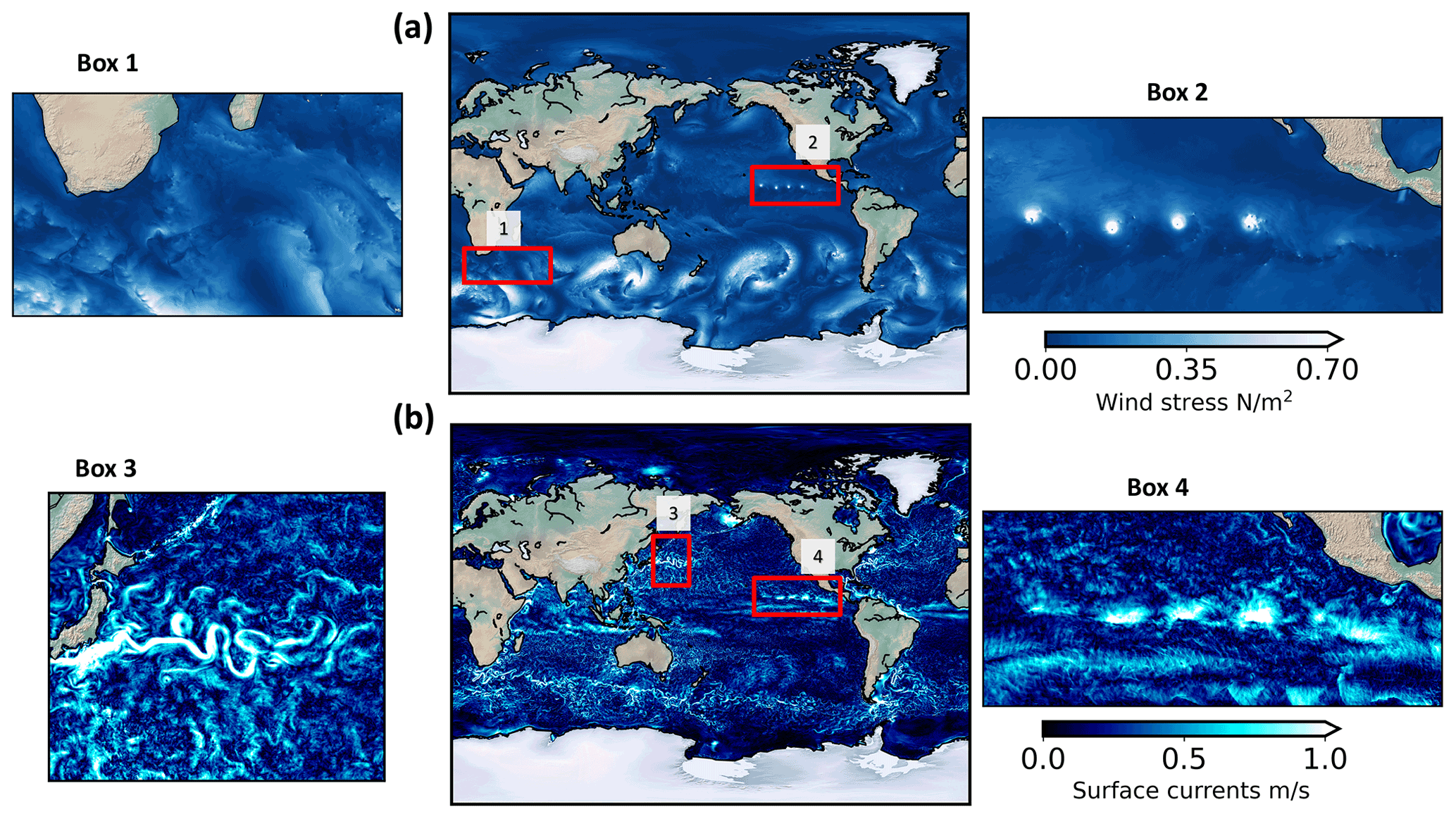
Figure 1(a) Snapshots of surface wind stress and (b) ocean-surface currents in the coupled ocean-atmosphere simulation (COAS) on 22 July, 12:00 GMT.
Figure 1a and b show a snapshot of wind stresses and ocean currents in the global ocean. Videos of these two key variables are available in https://doi.org/10.5281/zenodo.6478679 (Torres, 2022b). The wind stress variations have large scales, 𝒪(1000 km) (Fig. 1a), resulting from atmospheric weather patterns that propagate rapidly, for example, going from South Africa to South America within 6–10 d (Fig. 1a). Embedded within these large-scale patterns are smaller scale patterns (as small as 100 km), some of them propagating with the large-scale ones, others being quasi-stationary (see Box 1 in Fig. 1a and the movie). The latter are mostly the signature of ocean currents on the wind stress and can be identified from watching the movie. The impact of land topography on the wind stress is also noticeable in the movies, in particular close to the east coast of Asia at mid-latitudes and the west coast of Mexico at the Equator. The latter may lead to the formation of hurricanes, such as those noticeable in Box 2 of Fig. 1a. Energetic ocean currents (Fig. 1b) are characterized by very small scales in contrast to the wind stress and move slowly as revealed in the movie (see also Box 3 on Fig. 1b). These motions are mostly associated with wavy and unstable baroclinic mean currents and eddies. Zonal jets are noticeable at the Equator and in tropical regions (Fig. 1b). Not surprisingly, hurricanes have a strong signature on surface currents (Box 4 in Fig. 1b). Ocean current patterns with larger scales, but containing less energy than small-scale currents, are also noticeable in the movie. These patterns propagate with large-scale atmospheric storms. They are the signature of near-inertial motions and internal waves driven by the large-scale wind stress.
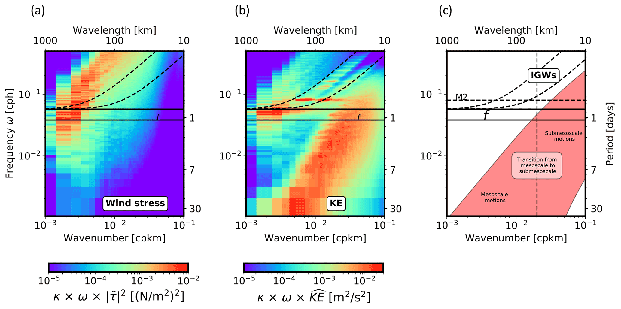
Figure 2COAS frequency-wavenumber spectra of (a) surface wind stress and (b) surface currents in the Kuroshio Extension region in winter. Panel (c) is a Stommel diagram of oceanic motions (see text). The dashed lines in the three panels show the linear dispersion relation curves for internal gravity waves (IGW) associated with the first four baroclinic modes, which helps to identify energetic internal gravity waves. See Torres et al. (2018) and Qiu et al. (2018) for a detailed explanation of the above partition.
3.2 Wind stresses and ocean currents in spectral space
The different temporal and spatial scales of wind stresses and ocean currents are further characterized in spectral space in regional domains. Figure 2 shows spectra of wind stresses and currents in the Kuroshio Extension region in the North Pacific (see Appendix A for spectra calculation details). The frequency and wavenumber ranges span periods between 2 h and 40 d and length scales from 10 km to 1000 km, respectively. Wind stresses and currents occupy different regions in spectral space. On the one hand, wind stresses (Fig. 2a) are mostly characterized by high frequencies (< 2 d) comprised of large spatial scales (> 500 km) for time scales larger than 12 h and small spatial scales (20–500 km) for time scales smaller than 12 h. Such wind stresses are the signature of large-scale atmospheric storms and the associated small-scale patterns that propagate with them. Small-scale wind stress patterns associated with slowly moving ocean eddies are weaker and occupy periods larger than 2 d. On the other hand, energetic ocean currents (Fig. 2b) are mostly characterized by smaller spatial scales (< 500 km) and lower frequencies (periods > 2 d). As sketched in Fig. 2c, these currents are associated with mesoscale eddies known to be driven by the baroclinic instability of mean currents. However, ocean currents also have a large magnitude in the near-inertial band (ω≈f) with scales larger than 500 km. These currents are associated with near-inertial waves (see Fig. 2c) forced by high-frequency winds.
Based on the properties discussed above, we analyzed the wind work over a 3-month period, during winter, spring, summer and fall to emphasize its seasonality. During each season, we consider the following decomposition for surface wind stress τ and ocean-surface currents uo:
where X represents either τ or uo, the overline operator represents a time average over 3 months, also called time mean or seasonal mean, and the prime operator represents time fluctuations with periods smaller than 3 months. The time fluctuations are further decomposed into a high-frequency component (hf) for periods smaller than 3 d and a low-frequency component (lf) for periods between 3 d and 3 months. Varying the 3 d threshold between low-frequency and high-frequency motions does not have a significant impact on the results of the present study. The hf component captures high-frequency contributions such as those at the inertial frequency. The lf component is further decomposed into two contributions in terms of spatial scales: the large-scale contribution (lf>) for spatial scales larger than a critical length scale Lc and the small-scale contribution (lf<) for scales smaller than Lc. Following Rai et al. (2021), we define Lc as the length scale for which the lf component of wind work is negative for scales smaller than Lc and positive for larger scales. Negative wind work at these scales has been referred to as “eddy killer” or “eddy damping”, a mechanism that has been thoroughly investigated during the past 15 years (Eden and Dietze, 2009; Renault et al., 2016, 2018; Rai et al., 2021). Using the same procedure as Rai et al. (2021), we found that Lc≈250 km (see Sect. 4.3 for more details).
3.3 Analysis of the wind work
The wind work depends not only on the amplitudes of time mean and fluctuating surface wind stress and currents but also on their cross-correlation. We apply the Reynolds decomposition to Eq. (2) using Eq. (3). The resulting wind work at each grid point averaged over 3 months includes a time-mean component () and a total time-dependent component (), such that
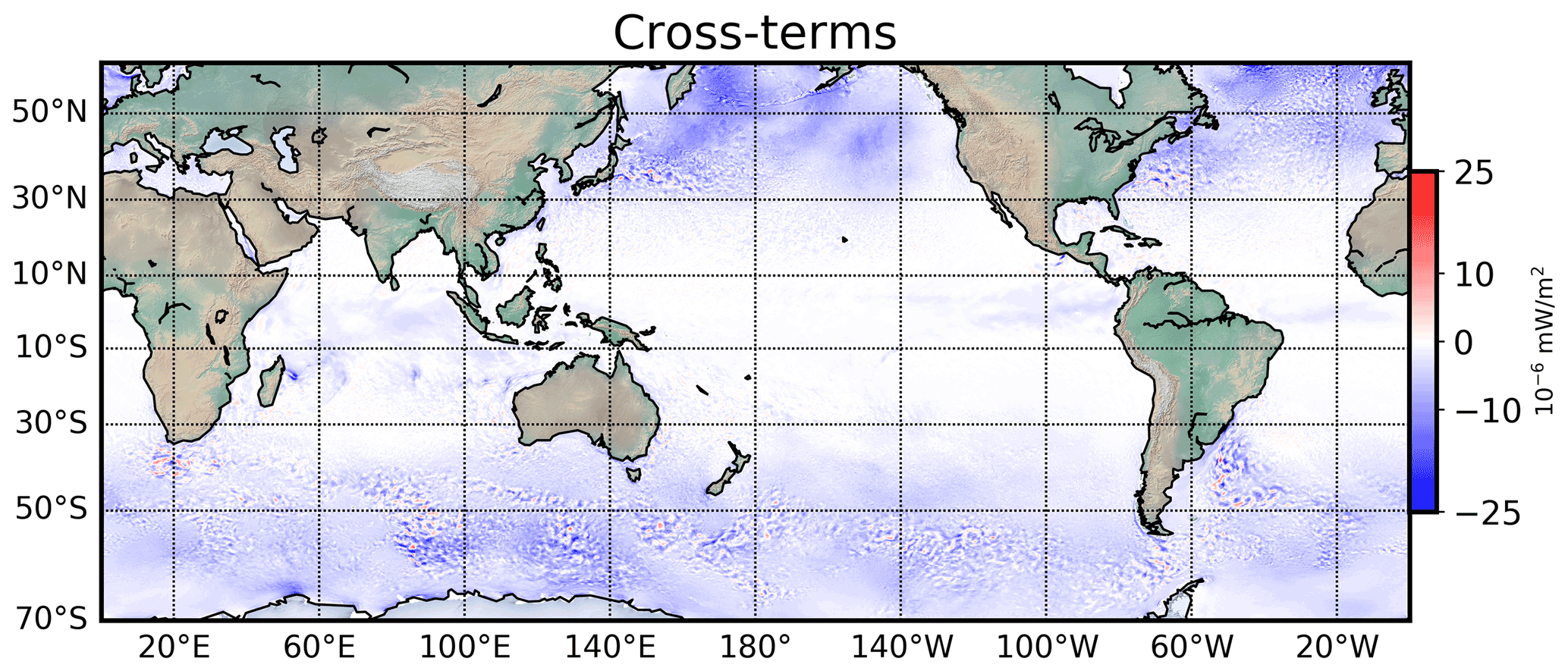
Figure 3The cross-terms not present in Eq. (4) estimated as the differences between the left and right hand sides of this equation.
First, we have checked the validity of the Reynolds decomposition by estimating the order of magnitude of each cross term not present in Eq. (4). Their order of magnitude is 10−6 smaller than the terms present in Eq. (4) (compare Fig. 3 with Fig. 4 and others), which confirms the pertinence of our decomposition. Estimation of these cross terms is consistent with the estimation found by Renault et al. (2020). The four terms on the right hand side (RHS) of Eq. (4) identify the contribution of the different time and spatial scales of the wind stress and current to the wind work averaged over 3 months. Each term in Eq. (4), associated with a given class of temporal and spatial fluctuations, directly forces surface currents corresponding to the same class as explained in Appendix B. Thus, the first term on the RHS in Eq. (4) should force mean currents (), the second one, mostly near-inertial waves and internal gravity waves (), the third one, large-scale currents and gyres (), and the last one, mesoscale eddies ().
However, each class of motions can be indirectly forced by the wind work associated with other time and spatial scales. This is due to the presence of the nonlinear advection terms in the momentum equations (see also Appendix B). Let us consider for example the equations for the time evolution of and where only nonlinear advection terms related to and are retained for the sake of simplicity (see Eq. B14 in Appendix B for a generalization),
where H is a mixed-layer depth assumed to be constant. From Eq. (5) surface currents, , are directly forced by . However, these currents are also affected by the first RHS term in Eq. (5) that involves . If currents are unstable production of surface currents at smaller spatial scales () can occur through this first RHS term. From Eq. (6), is directly forced by . The consequence is that through the first RHS term in Eq. (5), is indirectly forced by . Of course, scale interactions are more complex and involve more frequencies and spatial scales as discussed at the end of Appendix B (see Eq. B14). Such nonlinear interactions enable the kinetic energy transfer between scales (inverse and direct kinetic energy cascades) as well as current instabilities. However, the present example illustrates that in order to understand the wind impact on the ocean dynamics, we need to consider the different components of the wind work displayed in Eq. (4) altogether, and not just focusing on one or two components. The present study analyzes all wind work components. A more thorough future study should be dedicated to the kinetic energy budget in the upper oceanic layers that involves both wind work forcing and nonlinear advection of momentum.
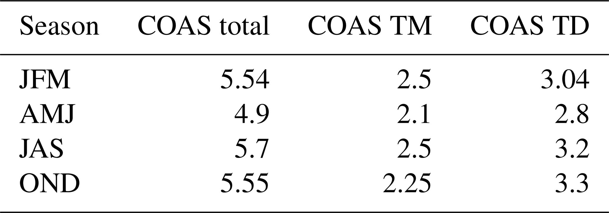
In this section we analyze the time-mean component of the wind work (first term on the RHS of Eq. 4) as well as the total time-dependent components (the last three terms on the RHS of Eq. 4). The total time-dependent components include the hf component and lf component (see Eq. 4). From Table 1, time-mean (COAS TM) and total time-dependent (COAS TD) components represent ∼ 44 % and ∼ 56 % of the total wind work, respectively. Their relative contributions as well as the total wind work (COAS total) vary weakly with the seasons. The total wind work is larger than 5 TW, a value close to recent estimations (Yu et al., 2018; Yu and Metzger, 2019). However, the spatial distribution of the different wind work components varies with the seasons, as discussed in the following subsections.
Table 1Contributions to the wind work of the time-mean (TM) component (first term on the RHS of Eq. 4) and total time-dependent (TD) component (last three terms on the RHS of Eq. 4) from COAS, over the World´s oceans, in terms of seasons: January–February–March (JFM), April–May–June (AMJ), July–August–September (JAS), and October–November–December (OND). Units are terawatts, TW.
4.1 Time-mean component:
Figure 4a–d and e display a significant seasonality of the time-mean component in each hemisphere, with the wind work intensified in fall and winter as compared to spring and summer, except at mid-latitudes in the Southern Hemisphere. The wind work, when zonally integrated at different latitudes (Fig. 4e), reach peak values of 2–2.5 GW in winter and 0.5 GW in summer. Wind work in tropical and equatorial regions has the same order of magnitude as the wind work at mid-latitudes.
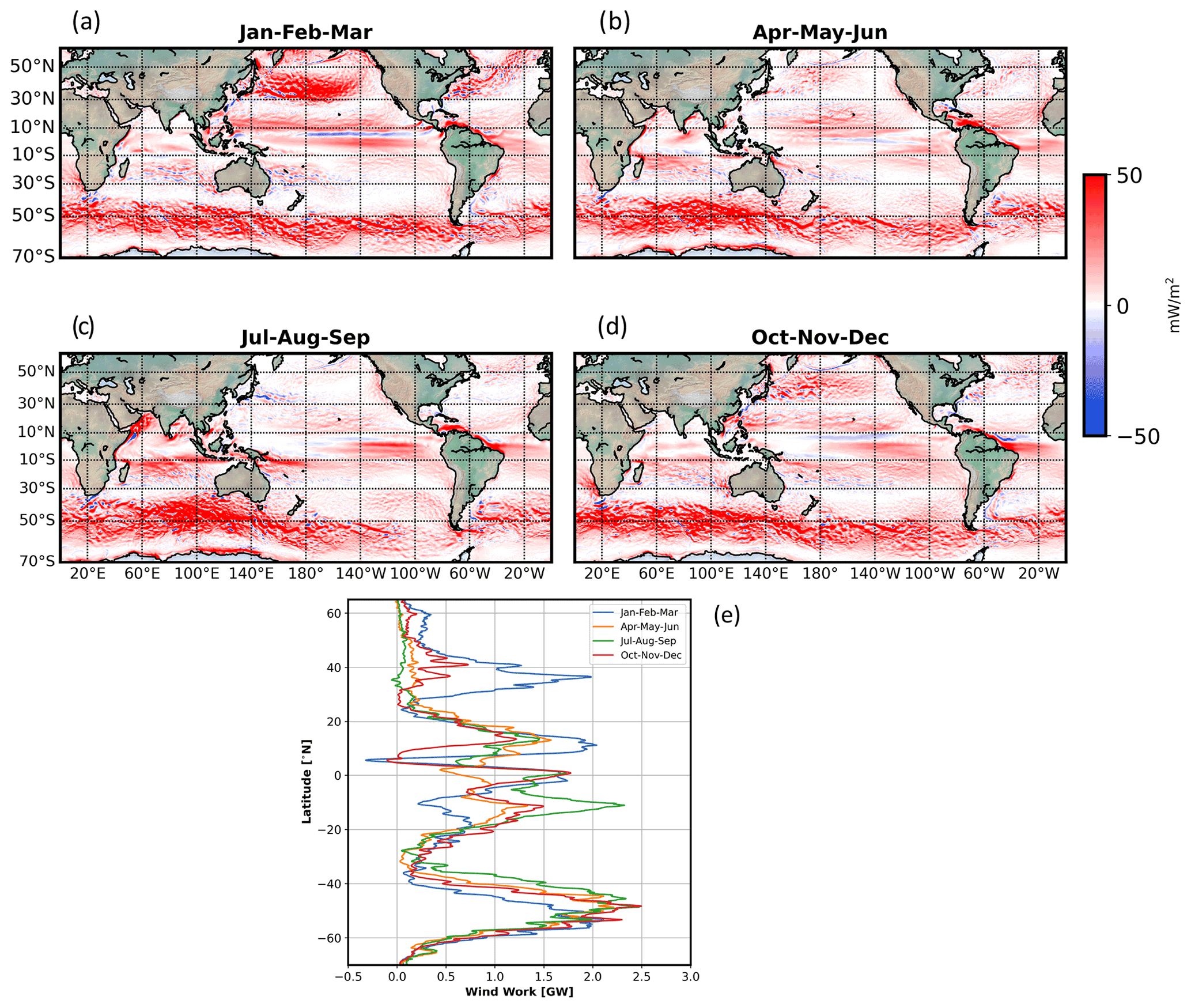
Figure 4(a–d) Time-mean component of the wind work, , in different seasons. (e) Wind work multiplied by the area of the numerical grid cell (m2) and zonally integrated during the four seasons.
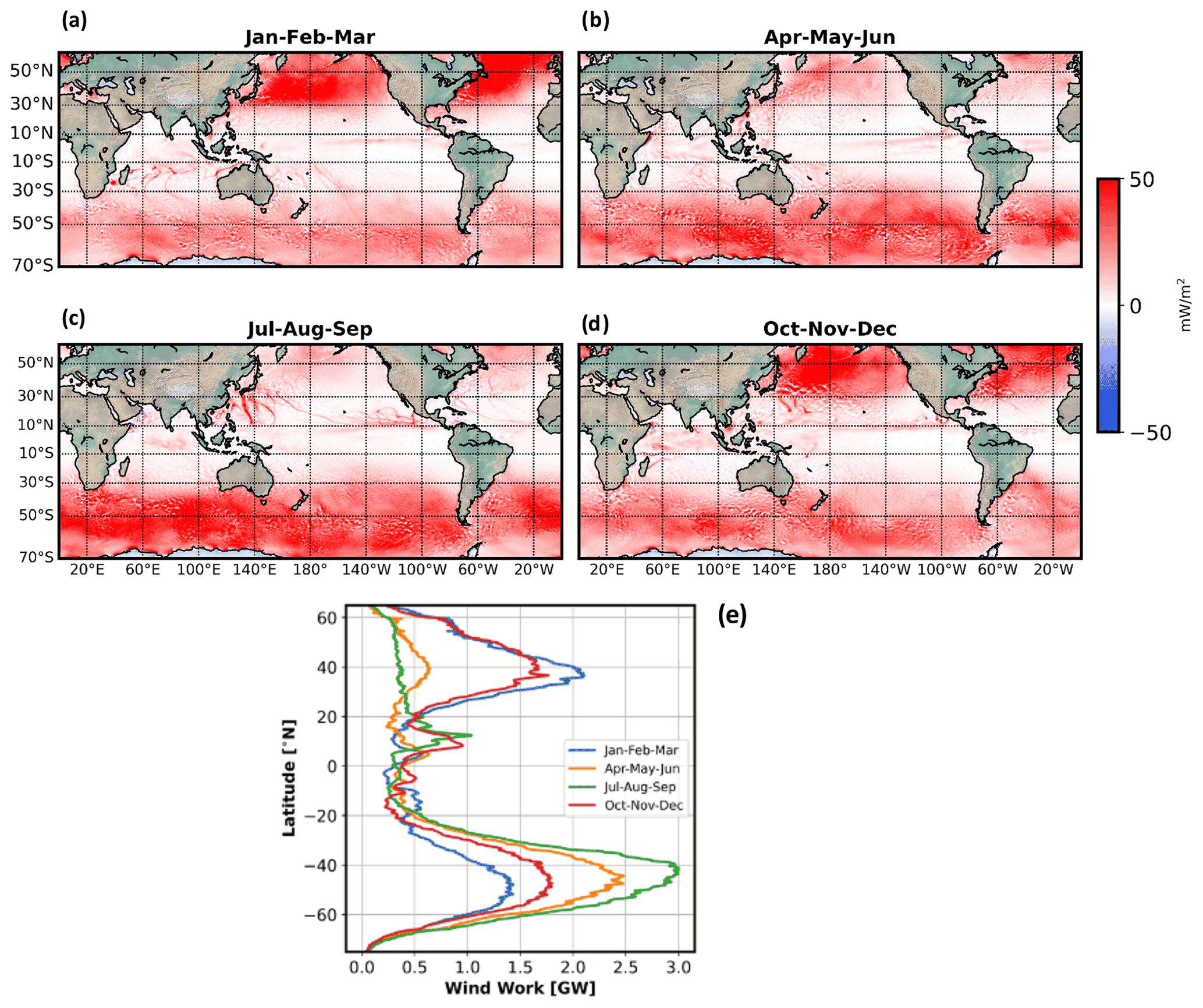
Figure 5(a–d) Time-dependent component of the wind work, , in different seasons. (e) Wind work multiplied by the area of the numerical grid cell (m2) and zonally integrated during the four seasons.
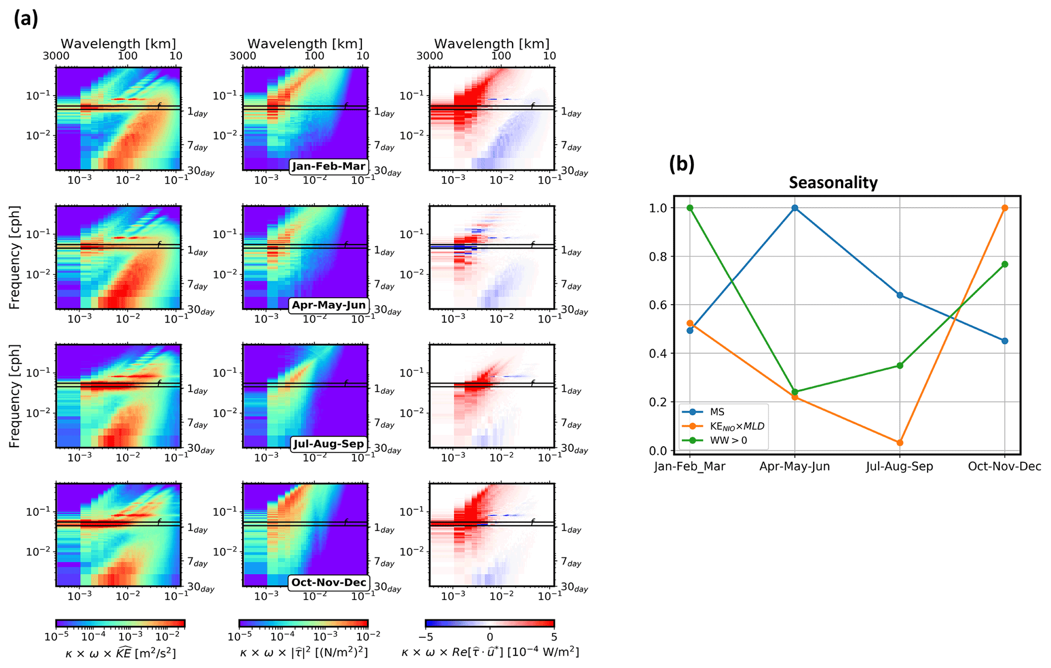
Figure 6(a) Seasonal variability of the frequency-wavenumber spectra of surface current (first column), wind stress (middle column), and co-spectrum of the wind work (third column). (b) Seasonal variability of kinetic energy associated with mesoscale motions, MS (defined by 350 km 30 km and periods 30 d 5 d, blue curve), kinetic energy of near-inertial motions times the mixed layer depth (orange curve), and positive wind work (green curve). The variance has been integrated then normalized to its maximum value.
In all seasons, wind work in tropical and equatorial latitudes, i.e., between 30∘ N and 30∘ S, displays several zonal patterns elongated over ∼ 3000 km mostly across the Indian, Pacific and Atlantic oceans with an intensification across the Equator (Fig. 4a–d). Such wind work, known to be associated with westward trade winds, impacts tropical and equatorial zonal jets (Maximenko et al., 2008; Chelton et al., 2011; Laurindo et al., 2017). The negative zonal band around 6∘ N is associated with the well-known eastward equatorial jet (Qiu et al., 2017). At these latitudes, wind work experiences a strong seasonality (Fig. 4a–d) because of the seasonality of the trade winds across the Equator. Wind work is also intensified south of 30∘ S, i.e., in the Antarctic Circumpolar Current (ACC), for instance around the longitude of 130∘ E, displaying elongated mesoscale patterns (100–400 km). These elongated mesoscale patterns are usually explained as the signature of the wind stress forcing on stationary mesoscale eddies trapped by topography as well as on eddies propagating eastward (Maximenko et al., 2008). Wind work at these southern mid-latitudes exhibits a weak seasonality because of the weak seasonality of the mean wind stress. However, wind work at northern mid-latitudes (north of 30∘ N) also exhibits a significant seasonality (Fig. 4e), as zonally elongated patterns at mesoscale (100–400 km, Fig. 4c) explained as the wind stress interacting with zonally propagating eddies in western boundary currents (WBCs) (Maximenko et al., 2008; Chelton et al., 2011). The small wind work observed in summer at northern mid-latitudes is due to weak summertime wind stresses off the east coast of Asia and west coast of America that weakly impact mesoscale eddies within WBCs.
4.2 Total time-dependent component of the wind work:
The total time-dependent component of the wind work (Fig. 5) that comprises the last three terms in Eq. (4), differs from that of the time-mean wind work (Fig. 4). The total time-dependent component is much weaker in tropical and equatorial regions (by a factor up to 3) and there is a strong seasonality in the Southern Hemisphere (compare Figs. 5e and 4e). In each hemisphere, at mid-latitudes (> 30∘ N and < 30∘ S) wind work is large in fall and winter (Fig. 5a, d) in the Northern Hemisphere (Southern Hemisphere Fig. 5b, c) and smaller in spring and summer (Fig. 5b, c) in the Northern Hemisphere (Southern Hemisphere Fig. 5a, d). This is confirmed by the zonally averaged wind work (panel e). This seasonality at mid-latitudes is explained by synoptic atmospheric storms (with time scales of a few days) that are intensified in winter. These characteristics are consistent with previous studies (Watanabe and Hibiya, 2002; Zhai, 2013; Yu et al., 2018). Also, the emergence of hurricanes in summer and fall, particularly in the Northern Hemisphere, have a strong signature on the wind work (see for example Fig. 5c, and also videos in https://doi.org/10.5281/zenodo.6478679 (Torres, 2022b).
The spectra of ocean current and wind stress for different seasons (first and second columns of Fig. 6a, respectively) in the Kuroshio Extension reveal how the different time and spatial scales associated with the wind work components vary seasonally. The effective spatial scales considered in these spectra are smaller than 1000 km and the time scales are smaller than 3 months. Within this time and spatial domain, ocean motions are dominated by near-inertial and higher frequency motions as well as by lower frequency mesoscale eddies (< 500 km). Currents with larger scales are weakly energetic in this region. The wind stress is found to be much weaker in spring and summer than in fall and winter. During fall and winter the wind stress has greater energy at higher frequencies (Fig. 6a, second column). High-frequency ocean currents, such as near-inertial oscillations (NIO) forced by the wind stress, exhibit a seasonality different from the wind stress: NIOs are energetic in summer and fall (third and fourth rows on Fig. 6a, first column) and weaker during winter and spring (first and second rows on Fig. 6a, first column). One explanation is that wind stress forces NIO kinetic energy integrated over the mixed-layer depth. Since the mixed-layer depth is smaller in summer than in winter, the velocities associated with the total mixed-layer NIO kinetic energy are larger in summer. This is confirmed when the surface NIO kinetic energy is multiplied by the mixed-layer depth: we recover a seasonality close to that of wind field and therefore of the wind work, as displayed on Fig. 6b. Ocean currents with low frequency, such as mesoscale eddies (with sizes larger than 100 km) and submesoscale structures, are less energetic in summer and fall compared with winter and spring (see Fig. 6b). Such seasonality of low-frequency ocean motions is consistent with previous studies (Sasaki et al., 2014; Qiu et al., 2018; Callies et al., 2015; Rocha et al., 2016). Indeed, submesoscales (< 50 km) become energetic in winter when the mixed-layer depth is large, with the kinetic energy of these scales being transferred to mesoscale eddies through the so-called inverse kinetic energy cascade, leading to higher mesoscale kinetic energy in spring (Sasaki et al., 2014; Lawrence and Callies, 2022).
From these wind work co-spectra, the total wind work is larger in fall and winter and smaller in spring and summer (Fig. 6b), consistent with Fig. 5. As illustrated on Fig. 6a (last column), the time-dependent wind work is mostly explained by the component that forces near-inertial motions and in particular by the magnitude of the wind stress. The part that forces mesoscale eddies and submesoscales, i.e., motions with lower frequency, is negative with a much smaller magnitude. This component is further discussed in the next section.
4.3 Low-frequency component of the wind work:
We now examine the low-frequency component of the wind work corresponding to wind stresses and ocean currents with periods larger than 3 d. Low-frequency ocean currents at mid-latitudes are often referred to as currents in geostrophic balance (balance between Coriolis and pressure gradients terms in the momentum equations), usually diagnosed from satellite altimetry (Chelton et al., 2011). The present numerical study includes, in addition, ageostrophic low-frequency currents (departing from geostrophy) that comprise ageostrophic eddy currents and surface wind-driven Ekman flow. These ageostrophic currents can explain 30–50 % of the total low-frequency currents in energetic areas (Qiu et al., 2014; Chassignet and Xu, 2017). However, we expect the correlation between wind stress and wind-driven Ekman flow to be larger than the correlation between wind stress and total eddy currents since the latter are mostly driven by the interior ocean dynamics.
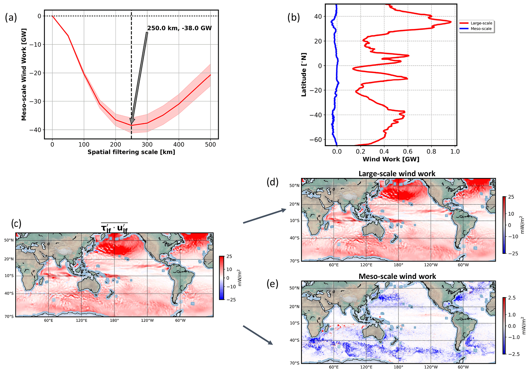
Figure 7Low-frequency wind work. (a) Partition into positive and negative wind work. Lc is defined as the minimum of the blue (COAS) (see Rai et al., 2021 for the calculation of these curves) using 12-month outputs of wind stresses and ocean currents. Interpretation of Lc is that all wind work with scales smaller (larger) than Lc is negative (positive). (b) Zonally integrated low-frequency wind work with scales larger (red curve) and smaller (blue curve) than Lc from COAS during the period April–May–June. (c, d, e) Distribution in physical space of the (c) low-frequency wind work from COAS for scales larger (d) and smaller (e) than Lc during the period April–May–June.
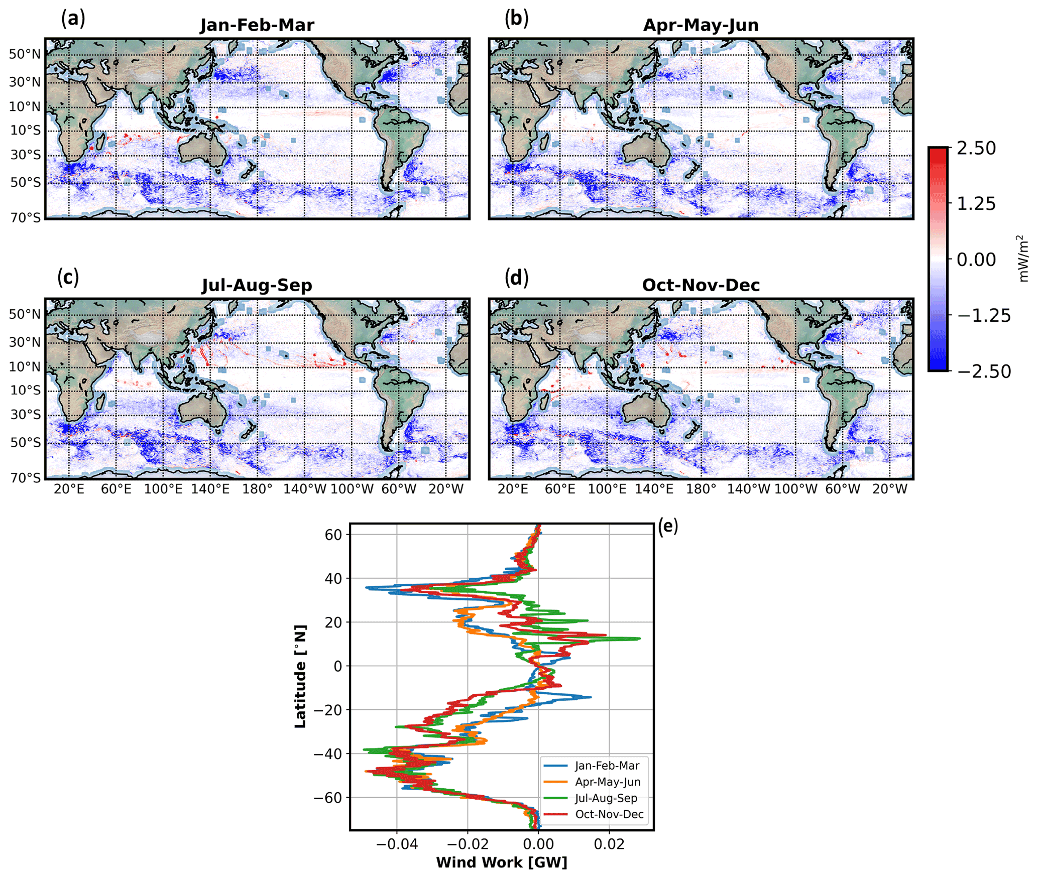
Figure 8(a–d) Low-frequency wind work with scales smaller than Lc averaged over a period of 3 months, . (e) Wind work multiplied by the area of the numerical grid cell (m2) and zonally integrated during four seasons.
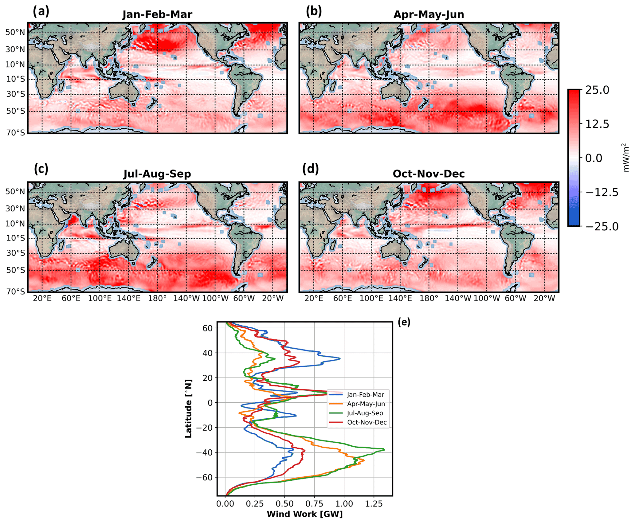
Figure 9(a–d) Low-frequency wind work with scales larger than Lc averaged over a period of 3 months, . (e) Wind work multiplied by the area of the numerical grid cell (m2) and zonally integrated during four seasons.
Referring to Eq. (4), the low-frequency component is decomposed into two parts using a critical length scale, Lc: the first part, ), corresponds to wind stresses and ocean currents with spatial scales larger than Lc and the other one, , corresponding to wind stresses and ocean currents with scales smaller than Lc. The value, Lc, is defined such that the low-frequency component of the wind work is negative for scales smaller than Lc and positive for larger scales. The methodology to determine Lc follows Rai et al. (2021). The low-frequency fields ( or ) are convolved with a window function G> (top-hat kernel to define) the low-frequency component with spatial scales larger than Lc: , where * is a convolution on a sphere as described in Aluie (2019). Then, the low-frequency component to the wind work of all spatial scales smaller than a given scale, L, has been estimated for the global ocean using 12-month outputs of wind stresses and ocean currents and is shown on Fig. 7a. As expected, the wind work is negative for small scales and reaches a minimum at L=Lc equal to 250 km for COAS simulation. This means that wind work for L<Lc is negative and becomes positive for L>Lc.
From Fig. 8a–d, (the wind work corresponding to scales <Lc) is negative in all seasons in most oceanic regions. This points to the eddy dampening effect explained by many studies (Eden and Dietze, 2009; Renault et al., 2016, 2018; Rai et al., 2021). An heuristic argument is that winds usually have scales larger than 500 km and therefore an approximation of the wind stress and wind work at small scales (L<Lc) is given by (using Eqs. 1 and 2):
More detailed arguments are found in Renault et al. (2017) and Rai et al. (2021). From Fig. 8a–d, the negative contribution of is found principally at mid-latitudes in regions of energetic mesoscale eddies, such as the ACC and WBC. Noticeably, this mid-latitude contribution does not vary seasonally as confirmed by the zonally integrated wind work (Fig. 8e). Its magnitude is not large enough to impact the total time-dependent wind work (Fig. 5e). In tropical and equatorial regions, a seasonality is observed (Fig. 8e) even revealing small regions with positive wind work. Such positive wind work cannot be explained by the arguments leading to Eq. (8). A closer look at Fig. 8a–d and at movies (https://doi.org/10.5281/zenodo.6478679, Torres, 2022b, in particular see the movie GEOS_ECCO_TAUSPEED.mp4) indicates that this positive wind work comes from the signature of hurricanes with a size smaller than Lc during summer and fall. However, this positive wind work has a much smaller magnitude than the negative wind work observed at mid-latitudes (Fig. 7e).
Comparison of Figs. 9a–d and 8a–d reveals that (the wind work corresponding to scales >Lc) differs greatly from , not only in terms of sign but also in terms of magnitude and seasonality. These figures indicate that the magnitude of is 10 times larger than and is closer to, although smaller by a factor 2, than the total time-dependent wind work (Figs. 5e and 9e). The strong seasonality of resembles the total time-dependent wind work. These results indicate that the total time-dependent wind work at mid-latitudes splits almost equally into high-frequency and low-frequency components. In tropical and equatorial regions, a comparison between Figs. 5e and 9e reveals that patterns have a comparable magnitude, indicating that the high-frequency component of the wind work is small at these latitudes. The positive contribution of at mid-latitudes, should strengthen large-scale low-frequency ocean currents. As emphasized by Chen et al. (2014) and Yang et al. (2021), shear and baroclinic instabilities of these large-scale currents may generate smaller scale eddy currents. This suggests that production of smaller scale eddies (L<Lc) by the positive part, , through instabilities may be larger than the eddy dampening as discussed in Sect. 3.2. This points to the importance of accounting for all wind work components to better infer the wind forcing of the ocean dynamics. The result also emphasizes that a full kinetic energy budget should account for all the wind work components as well as the nonlinear advection terms in the momentum equations, as the instabilities mentioned before are explained by these terms.
4.4 High-frequency component of the wind work:
From Eq. (4), the high-frequency component of the wind work is just the difference between the total time-dependent component (Fig. 5e) and the low-frequency component, the latter being dominated by the large-scale component (Fig. 9e). High-frequency and low-frequency components are dominant at mid-latitudes, i.e., at the location of atmospheric storm tracks, and have similar magnitudes as noted in the previous section. High-frequency winds are expected to force ocean currents principally at the inertial frequency as the ocean is an oscillator with the frequency f. A strong forcing means that near-inertial motions should be in phase with wind stresses (Klein et al., 2004; Alford et al., 2016). To diagnose the phase relationship between high-frequency wind stresses and near-inertial and higher frequency ocean motions, we have re-estimated the total time-dependent component of the wind work in the global ocean by applying a phase lag of 12 h between wind stresses and currents. Results (not shown) indicate that the resulting high-frequency component is reduced by a factor close to 10 at mid-latitudes when integrated zonally in both hemispheres, with the new total time-dependent component now close to the low-frequency component. This result highlights that wind stresses and ocean currents are largely in phase at short time scales.
To further understand the impact of high-frequency wind stress on the wind work, we have tested this phase relationship in spectral space, focusing on the Kuroshio Extension region. Figure 10a shows the wind work co-spectrum estimated from the coupled simulation. As expected, the co-spectrum reveals a positive maximum around the inertial and higher frequencies, which corresponds to the forcing of near-inertial and higher frequency motions (Klein et al., 2004; Alford et al., 2016). The magnitude of the wind work for these high frequencies (in terms of period, T<3 d) is 52 mW m−2. For time scales larger than 3 d, the wind work is negative (Fig. 10a). This is related to the mesoscale eddy dampening mentioned before, as low-frequency ocean motions in the Kuroshio Extension are mostly associated with mesoscale eddies and not large-scale currents. In terms of negative wind work, the magnitude is −16 mW m−2. Considering positive and negative wind work, the net wind work is positive and equal to 36 mW m−2.
Similar results have been found in other areas of the world's oceans, such as the ACC, the Gulf Stream and tropical regions (see Fig. 11).
We repeated this spectral calculation by applying a phase lag of 12 h between wind stresses and ocean currents. Results (see the comparison of Fig. 10a and b) indicate that the 12 h offset impacts the wind work in the high-frequency band. In this spectral band the wind work now displays alternating positive and negative values. The wind work that impacts low frequency motions is almost unchanged by the offset. As a result the total wind work is slightly negative. Similar results (not shown) are obtained using a 3 h or 6 h offset. This test emphasizes not only the spatial collocation of wind stress and currents, but also their contemporaneity, which has an impact on the integrated wind work.
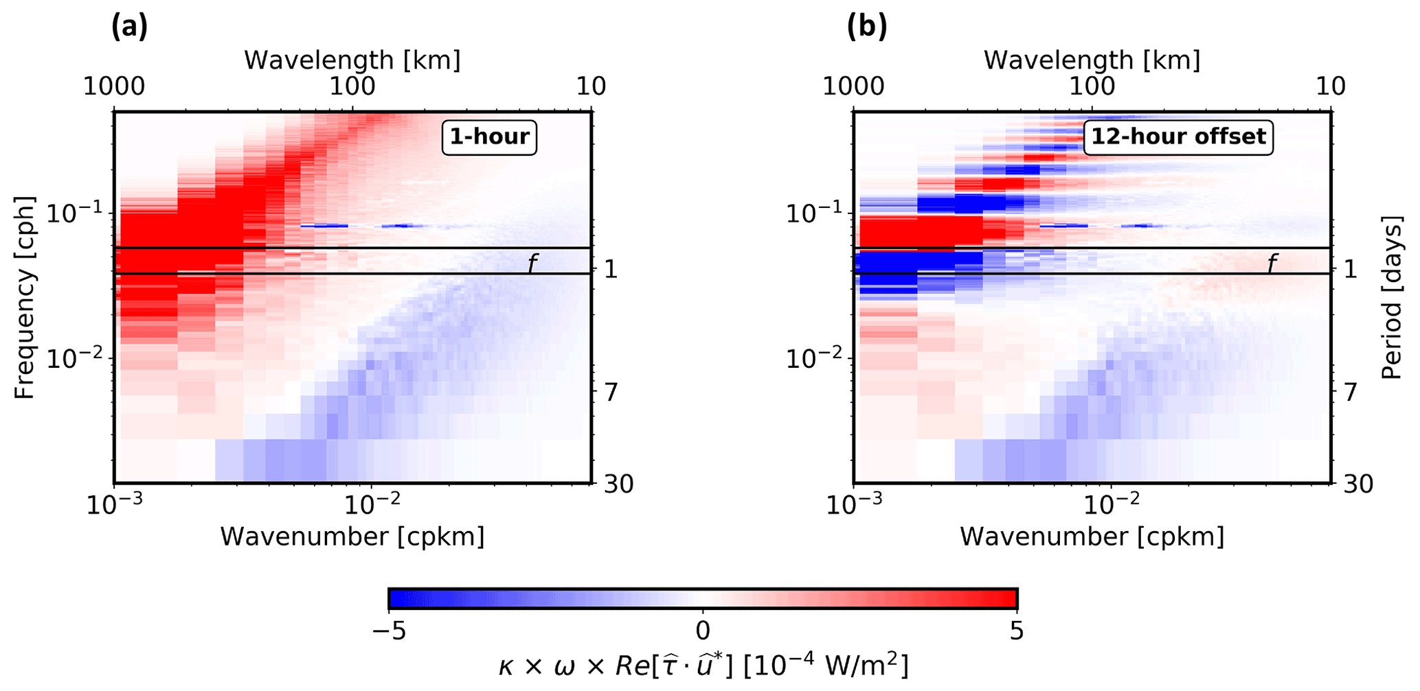
Figure 10(a) Co-spectrum of wind stresses and surface ocean currents in the Kuroshio Extension region from COAS simulation. (b) Same as (a) except by off-setting wind stresses and surface currents by 12 h. Using different off-settings (3 and 6 h) produce the same results at 12 h.
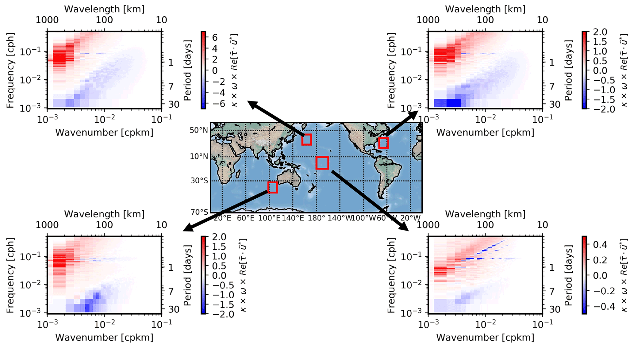
Figure 11Co-spectrum of wind stresses and surface ocean currents in several regions from the COAS simulation (see square boxes in the middle panel). Note the color range is different in each panel.
The scalar product of wind stress and ocean surface current, called wind work, is the kinetic energy transfer between the ocean and the atmosphere. Our study has examined the impact of the wind work on the forcing of ocean currents using outputs of wind stresses and currents from a new coupled ocean-atmosphere simulation with high spatial resolution. The resulting wind stresses and surface ocean currents involve a broad range of time and space scales, from 1 h to 1 year and 10 km to more than 3000 km. Our examination makes use of a simple method that splits the wind work into three components. (i) The high-frequency component, corresponding to wind stress and ocean currents with time scales less than 3 d, (ii) the low-frequency component, corresponding to wind stress and ocean currents with time scales between 3 d and 3 months, and (iii) the time-mean or seasonal-mean component diagnosed from wind stress and ocean currents averaged over 3 months. Each of these three components, when integrated over the world's oceans, does not vary much with seasons and explains 28 % of the total wind work for the first 2 components and 44 % for the third one. This leads to a total wind work larger than 5 TW, a value close to recent estimations (Yu et al., 2018; Yu and Metzger, 2019). However, the analysis in physical and spectral spaces of each of these components reveals a strong diversity of their characteristics.
The high-frequency component of the wind work (time scales smaller than 3 d) dominates in regions of mid-latitude atmospheric storm tracks where it directly forces internal gravity waves, mostly near-inertial oscillations with large spatial scales. One important characteristic of this component is its sensitivity to the phase relationship between wind stresses and ocean currents. Thus, a spectral analysis shows that a phase shift of 3–12 h between wind stress and ocean currents, reduces this component by a factor of up to 10. The high frequency component also has a strong seasonality because of winter atmospheric storms.
The low-frequency component (corresponding to wind stress and ocean currents with time scales between 3 d and 3 months) has been analyzed following the approach of Rai et al. (2021), which consists of defining a critical length scale that splits this component into a negative small-scale part and a positive large-scale part. The positive part exhibits a strong seasonality at mid-latitudes, not present in the negative part. In addition, the magnitude of the positive part is 10 times larger than the negative part. These characteristics of the wind work, not found when using geostrophic currents diagnosed from altimetry datasets, point to the importance of low-frequency ageostrophic current contribution to the wind work (Rai et al., 2021). The large magnitude of the positive part may be explained by the strong correlation between wind stress and wind-driven Ekman flow. Confirmation of this explanation will be the focus of a future study. The small-scale part acts as an eddy dampening for mesoscale eddies as discussed before (Eden and Dietze, 2009; Renault et al., 2016, 2018). This eddy dampening effect may be counterbalanced by the positive large-scale part of the wind work. Indeed, instabilities of larger scale currents may energize currents associated with smaller eddies (L< 250 km). Reciprocally, smaller eddies can energize larger eddies through an inverse kinetic energy cascade. This emphasizes that the two low-frequency parts of the wind work cannot be examined separately, but need to be examined through a full kinetic energy budget, a focus of a future work.
The time-mean or seasonal-mean component is significant in equatorial and tropical regions as well as at mid-latitudes. This component forces equatorial and tropical zonal jets as well as stationary and propagating large eddies. It may also force tropical wave instabilities through nonlinear advection terms, but this still has to be assessed using a full kinetic budget as mentioned before.
Our results emphasize the need to have satellite observations of wind stresses and currents that are collocated and contemporaneous with a resolution of at least 10 km and a temporal resolution less than 12 h. The present ASCAT wind observations and ocean currents diagnosed from conventional altimeters do not meet these requirements. However, several future projects, such as the wind and current mission (Odysea) (Rodríguez et al., 2019) and the Ocean Surface Current Multiscale Observation Mission (OSCOM) (Du et al., 2021), intend to address the limitations of existing wind stress and ocean current products. The Odysea mission aims to measure wind stresses and ocean surface currents (including both geostrophic and ageostrophic currents) with sensors on board a single satellite, with a spatial and temporal resolution of ∼ 10 km and twice a day. In addition to being collocated and contemporaneous, these global measurements of wind stress and ocean currents will have wide swaths as large as ∼1800 km. Observations from the upcoming Surface Water and Ocean Topography(SWOT) mission should enable the diagnosis of geostrophic currents with a resolution of ∼ 15 km over a wide swath of 120 km (Fu and Ferrari, 2008; Wang et al., 2019). Combining Odysea and SWOT observations should enable assessment of the relative contributions of geostrophic and ageostrophic currents to the wind work. We envision that these future observations, exploited in combination with SST observations from the advanced microwave scanning radiometer (AMSR-E), will permit estimates of not only the kinetic energy budget (including the wind work and nonlinear advection of momentum), as suggested by the present study, but also the heat budget in the upper oceans (Klein et al., 2019). Modeling studies like the present one should help to make a better assessment of the potential of these missions.
The ω-κ spectrum of a given variable is computed in a domain 1000 km in size and over 90 d. We refer the reader to Torres et al. (2018) for the full methodology. Briefly, before computing the ω-k spectrum of a , its linear trend is removed and a 3-D Hanning window is subsequently applied to the detrended (Qiu et al., 2018). A discrete 3-D Fourier transform is then computed to retrieve the Fourier coefficients, where is the Fourier transform, k the zonal wavenumber, l the meridional wavenumber, and ω the frequency. Finally, the 3-D Fourier transform is used to compute a 2-D spectral density, where κ is the isotropic wavenumber defined as . The transformation from an anisotropic spectrum to an isotropic spectrum is performed following the methodology described by Torres et al. (2018).
The co-spectrum of the wind work is computed similarly to the ω-κ spectrum, following the methodology described in Flexas et al. (2019). First, the Fourier transforms of the wind stress and ocean current are calculated. The co-spectrum of the wind work is then given by
where Re is the real part of the complex quantity, and the asterisk (*) the complex conjugate. The 2-D co-spectrum, , is retrieved using the procedure described in the first paragraph of this Appendix.
The ω-κ spectrum and co-spectrum are presented in a variance preserving form for easier comparison across the frequency-wavenumber domain.
Let us assume a constant mixed-layer depth, H, for the sake of simplicity. Wind stress, τ, will force surface currents, uo, following
Using and , with overline being a time-average operator over 3.5 months, leads to
Time-averaging Eq. (B2) and multiplying the resulting equation by yields
After multiplying Eq. (B2) by and taking the time average and using Eq. (B3), we get
The same operation can now be done using , which leads to
The same arguments, but now in spatial space, can be applied using leading to
Thus, from Eqs. (B3), (B5), (B6), (B7), and (B8), each term on the RHS of Eq. (4), related to a given fluctuation class, directly forces surface currents corresponding to the same class. The results above can also be understood if moving to the spectral space, as Eq. (B1) becomes
leading to
with the Fourier transform, * the conjugate, ω the frequency, k the wavenumber and ℛ the real part. Therefore, each frequency and each wavenumber of the wind stress forces surface currents with the same frequency and wavenumber.
However, the full momentum equations, including nonlinear advection terms, highlight that fluctuating wind stresses indirectly force mean surface currents and similarly mean wind stresses force fluctuating surface currents. These nonlinear effects are illustrated below.
Let us start with the full momentum equations
Applying, for example, the decomposition and to Eq. (B11) leads, after some calculations, to
From Eqs. (B12) and (B13), the time-mean and fluctuations surface currents, resulting directly from the wind work forcing, subsequently interact through the nonlinear advection terms in the momentum equations. For example, fluctuating surface currents forced by wind stress fluctuations (Eq. B13) impact the mean current through the second RHS term in Eq. (B12). Similarly, the mean current forced by the mean wind stress (Eq. B12) impacts current fluctuations through the first RHS term in Eq. (B13) as these mean currents can be unstable. This example emphasizes that mean wind stress can force indirectly fluctuating currents and fluctuating wind stress can force indirectly mean currents. It confirms that the different components of the wind work displayed in Eq. (4) need to be considered altogether and not separately. Nonlinear interactions are more complex than shown in Eqs. (B12) and (B13). This can be understood when moving again to the spectral space. Indeed, the generalization of Eq. (B10) leads to
where uo in the term involve frequencies (ω1 and ω2) and wavenumbers (k1 and k2) such that and .
The exact version of the model used to produce the results used in this paper is archived on Zenodo (https://doi.org/10.5281/zenodo.6686083, Torres, 2022a), as are input data and scripts to run the model and produce the plots.
The coupled ocean-atmosphere simulation can be found at: https://portal.nccs.nasa.gov/datashare/G5NR/DYAMONDv2/GEOS_6km_Atmosphere-MITgcm_4km_Ocean-Coupled/GEOSgcm_output/ (NASA, 2022). In particular, the dataset contained in the folder geosgcm_surf/ was used in this study. The variables used in this study are U (east-west velocity component), V (north-south velocity component), oceTAUX (east-west wind stress component), and oceTAUY (north-south wind stress component).
Videos at https://doi.org/10.5281/zenodo.6478679 (Torres, 2022b) display surface ocean currents (zenodo/GEOS_ECCO_SSSPEED.mp4) and surface wind stress (zenodo/GEOS_ECCO_TAUSPEED.mp4).
HST and PK led the data analysis and data interpretation and drafted the manuscript. DM, CNH, AM, and ES helped develop and integrate the coupled ocean-atmosphere simulation. All authors contributed to the scientific interpretation of the results and reviewed the manuscript.
The contact author has declared that none of the authors has any competing interests.
Publisher’s note: Copernicus Publications remains neutral with regard to jurisdictional claims in published maps and institutional affiliations.
This research was carried out in part at the Jet Propulsion Laboratory, California Institute of Technology, under a contract with the National Aeronautics and Space Administration (NASA) and funded through the internal Research and Technology Development program. Hector S. Torres, Jinbo Wang, Alexander Wineteer, Ernesto Rodriguez, Dimitris Menemenlis, Hong Zhang, and Dragana Perkovic-Martin were supported by the NASA Physical Oceanography (PO) and Modeling, Analysis, and Prediction (MAP) programs. Andrea Molod, Christopher N. Hill, and Ehud Strobach also received funding from NASA MAP. Patrice Klein acknowledges support from the SWOT Science Team, the NASA S-Mode project, and the QuikSCAT mission. Andrew F. Thompson and Mar Flexas were supported by the NASA S-MODE project, award number 80NSSC19K1004, and PDRDF funding from NASA's Jet Propulsion Laboratory. Bo Qiu acknowledges support from the NASA OSTST project.
High-end computing was provided by the NASA Advanced Supercomputing (NAS) Division at the Ames Research Center.
This paper was edited by Riccardo Farneti and reviewed by two anonymous referees.
Alford, M. H., MacKinnon, J. A., Simmons, H. L., and Nash, J. D.: Near-inertial internal gravity waves in the ocean, Annu. Rev. Mar. Sci., 8, 95–123, 2016. a, b, c
Aluie, H.: Convolutions on the sphere: commutation with differential operators, GEM – International Journal on Geomathematics, 10, 1–31, 2019. a
Arbic, B. K., Alford, M. H., Ansong, J. K., Buijsman, M. C., Ciotti, R. B., Farrar, J. T., Hallberg, R. W., Henze, C. E., Hill, C. N., Luecke, C. A., Menemenlis, D., Metzger, E. J., Müeller, M., Nelson, A. D., Nelson, B. C., Ngodock, H. E., Ponte, R. M., Richman, J. G., Savage, A. C., Scott, R. B., Shriver, J. F., Simmons, H. L., Souopgui, I., Timko, P. G., Wallcraft, A. J., Zamudio, L., and Zhao, Z.: A Primer on Global Internal Tide and Internal Gravity Wave Continuum Modeling in HYCOM and MITgcm, in: New Frontiers in Operational Oceanography, edited by: Chassignet, E. P., Pascual, A., Tintoré, J., and Verron, J., chap. 13, GODAE OceanView, 307–392, https://doi.org/10.17125/gov2018.ch13, 2018. a
Callies, J., Ferrari, R., Klymak, J. M., and Gula, J.: Seasonality in submesoscale turbulence, Nat. Commun., 6, 6862, https://doi.org/10.1038/ncomms7862, 2015. a
Chassignet, E. P. and Xu, X.: Impact of horizontal resolution (1/12 to 1/50) on Gulf Stream separation, penetration, and variability, J. Phys. Oceanogr., 47, 1999–2021, 2017. a
Chelton, D. B., Schlax, M. G., and Samelson, R. M.: Global observations of nonlinear mesoscale eddies, Prog. Oceanogr., 91, 167–216, 2011. a, b, c
Chen, R., Flierl, G. R., and Wunsch, C.: A description of local and nonlocal eddy–mean flow interaction in a global eddy-permitting state estimate, J. Phys. Oceanogr., 44, 2336–2352, 2014. a
Clarke, R.: Observational studies in the atmospheric boundary layer, Q. J. Roy. Meteor. Soc., 96, 91–114, 1970. a
Du, Y., Dong, X., Jiang, X., Zhang, Y., Zhu, D., Sun, Q., Wang, Z., Niu, X., Chen, W., Zhu, C., Jing, Z., Tang, S., Li, Y., Chen, J., Chu, X., Xu, C., Wang, T., He, Y., and Peng, S.: Ocean surface current multiscale observation mission (OSCOM): Simultaneous measurement of ocean surface current, vector wind, and temperature, Prog. Oceanogr., 193, 102531, https://doi.org/10.1016/j.pocean.2021.102531, 2021. a
Eden, C. and Dietze, H.: Effects of mesoscale eddy/wind interactions on biological new production and eddy kinetic energy, J. Geophys. Res.-Oceans, 114, C05023, https://doi.org/10.1029/2008JC005129, 2009. a, b, c, d
Ferrari, R. and Wunsch, C.: Ocean circulation kinetic energy: Reservoirs, sources, and sinks, Annu. Rev. Fluid Mech., 41, 253–282, https://doi.org/10.1146/annurev.fluid.40.111406.102139, 2009. a
Flexas, M. M., Thompson, A. F., Torres, H. S., Klein, P., Farrar, J. T., Zhang, H., and Menemenlis, D.: Global Estimates of the Energy Transfer From the Wind to the Ocean, With Emphasis on Near-Inertial Oscillations, J. Geophys. Res.-Oceans, 124, 5723–5746, https://doi.org/10.1029/2018JC014453, 2019. a, b
Fu, L.-L. and Ferrari, R.: Observing oceanic submesoscale processes from space, Eos, T. Am. Geophys. Un., 89, 488–488, 2008. a
Garfinkel, C. I., Molod, A. M., Oman, L. D., and Song, I.-S.: Improvement of the GEOS-5 AGCM upon updating the air-sea roughness parameterization, Geophys. Res. Lett., 38, l18702, https://doi.org/10.1029/2011GL048802, 2011. a, b
Helfand, H. M. and Schubert, S. D.: Climatology of the Simulated Great Plains Low-Level Jet and Its Contribution to the Continental Moisture Budget of the United States, J. Climate, 8, 784–806, https://doi.org/10.1175/1520-0442(1995)008<0784:COTSGP>2.0.CO;2, 1995. a, b
Klein, P., Lapeyre, G., and Large, W.: Wind ringing of the ocean in presence of mesoscale eddies, Geophys. Res. Lett., 31, L15306, https://doi.org/10.1029/2004GL020274, 2004. a, b, c
Klein, P., Lapeyre, G., Siegelman, L., Qiu, B., Fu, L.-L., Torres, H., Su, Z., Menemenlis, D., and Le Gentil, S.: Ocean-Scale Interactions From Space, Earth Space Sci., 6, 795–817, https://doi.org/10.1029/2018EA000492, 2019. a, b
Komori, N., Ohfuchi, W., Taguchi, B., Sasaki, H., and Klein, P.: Deep ocean inertia-gravity waves simulated in a high-resolution global coupled atmosphere–ocean GCM, Geophys. Res. Lett., 35, L04610, https://doi.org/10.1029/2007GL032807, 2008. a
Kondo, J.: Air-sea bulk transfer coefficients in diabatic conditions, Bound.-Lay. Meteorol., 9, 91–112, 1975. a
Large, W. and Pond, S.: Open ocean momentum flux measurements in moderate to strong winds, J. Phys. Oceanogr., 11, 324–336, 1981. a
Large, W. G. and Yeager, S. G.: Diurnal to decadal global forcing for ocean and sea-ice models: The data sets and flux climatologies, NCAR Tech Note NCAR/TN-460+STR, 434, Boulder, Colo. Natl. Cent. for Atmos. Res., 2004. a
Large, W. G., McWilliams, J. C., and Doney, S. C.: Oceanic vertical mixing: A review and a model with a nonlocal boundary layer parameterization, Rev. Geophys., 32, 363–403, 1994. a
Laurindo, L. C., Mariano, A. J., and Lumpkin, R.: An improved near-surface velocity climatology for the global ocean from drifter observations, Deep-Sea Res. Pt. I, 124, 73–92, 2017. a
Lawrence, A. and Callies, J.: Seasonality and spatial dependence of meso-and submesoscale ocean currents from along-track satellite altimetry, J. Phys. Oceanogr., 52, 2069–2089, https://doi.org/10.1175/JPO-D-22-0007.1, 2022. a
Maximenko, N. A., Bang, B., and Sasaki, H.: Observational evidence of alternating zonal jets in the world ocean, Geophys. Res. Lett., 32, 2069–2089, https://doi.org/10.1175/JPO-D-22-0007.1, 2005. a
Maximenko, N. A., Oleg, V., M., Pearn, P., N., and Hideharu, S.: Stationary mesoscale jet-like features in the ocean, Geophys. Res. Lett., 35, L08603, https://doi.org/10.1029/2008GL033267, 2008. a, b, c
Molod, A., Suarez, M., and Partyka, G.: The impact of limiting ocean roughness on GEOS-5 AGCM tropical cyclone forecasts, Geophys. Res. Lett., 40, 411–416, https://doi.org/10.1029/2012GL053979, 2013. a, b
Molod, A., Takacs, L., Suarez, M., and Bacmeister, J.: Development of the GEOS-5 atmospheric general circulation model: evolution from MERRA to MERRA2, Geosci. Model Dev., 8, 1339–1356, https://doi.org/10.5194/gmd-8-1339-2015, 2015. a
NASA Goddard Space Flight Center: GEOS_6km_Atmosphere-MITgcm_4km_Ocean-Coupled, https://portal.nccs.nasa.gov/datashare/G5NR/DYAMONDv2/GEOS_6km_Atmosphere-MITgcm_4km_Ocean-Coupled/GEOSgcm_output/ last access: 28 October 2022. a
Nikurashin, M., Vallis, G. K., and Adcroft, A.: Routes to energy dissipation for geostrophic flows in the Southern Ocean, Nat. Geosci., 6, 48–51, 2013. a
Panofsky, H. A., Tennekes, H., Lenschow, D. H., and Wyngaard, J.: The characteristics of turbulent velocity components in the surface layer under convective conditions, Bound.-Lay. Meteorol., 11, 355–361, 1977. a
Polzin, K. L. and Lvov, Y. V.: Toward regional characterizations of the oceanic internal wavefield, Rev. Geophys., 49, RG4003, https://doi.org/10.1029/2010RG000329, 2011. a
Qiu, B., Chen, S., Klein, P., Sasaki, H., and Sasai, Y.: Seasonal mesoscale and submesoscale eddy variability along the North Pacific Subtropical Countercurrent, J. Phys. Oceanogr., 44, 3079–3098, 2014. a
Qiu, B., Nakano, T., Chen, S., and Klein, P.: Submesoscale transition from geostrophic flows to internal waves in the northwestern Pacific upper ocean, Nat. Commun., 8, 1–10, 2017. a
Qiu, B., Chen, S., Klein, P., Wang, J., Torres, H., Fu, L.-L., and Menemenlis, D.: Seasonality in transition scale from balanced to unbalanced motions in the world ocean, J. Phys. Oceanogr., 48, 591–605, 2018. a, b, c
Rai, S., Hecht, M., Maltrud, M., and Aluie, H.: Scale of oceanic eddy killing by wind from global satellite observations, Sci. Adv., 7, eabf4920, https://doi.org/10.1126/sciadv.abf4920, 2021. a, b, c, d, e, f, g, h, i, j
Renault, L., Molemaker, M. J., McWilliams, J. C., Shchepetkin, A. F., Lemarié, F., Chelton, D., Illig, S., and Hall, A.: Modulation of wind work by oceanic current interaction with the atmosphere, J. Phys. Oceanogr., 46, 1685–1704, 2016. a, b, c, d
Renault, L., McWilliams, J. C., and Masson, S.: Satellite observations of imprint of oceanic current on wind stress by air-sea coupling, Sci. Rep., 7, 1–7, 2017. a
Renault, L., McWilliams, J., and Gula, J.: Dampening of Submesoscale Currents by Air-Sea Stress Coupling in the Californian Upwelling System, Sci. Rep., 8, 13388, https://doi.org/10.1038/s41598-018-31602-3, 2018. a, b, c
Renault, L., Masson, S., Arsouze, T., Madec, G., and Mcwilliams, J. C.: Recipes for how to force oceanic model dynamics, J. Adv. Model. Earth Sy., 12, e2019MS001715, https://doi.org/10.1029/2019MS001715, 2020. a
Rimac, A., von Storch, J.-S., Eden, C., and Haak, H.: The influence of high-resolution wind stress field on the power input to near-inertial motions in the ocean, Geophys. Res. Lett., 40, 4882–4886, 2013. a
Rocha, C. B., Gille, S. T., Chereskin, T. K., and Menemenlis, D.: Seasonality of submesoscale dynamics in the Kuroshio Extension, Geophys. Res. Lett., 43, 11–304, 2016. a
Rodríguez, E., Bourassa, M., Chelton, D., Farrar, J. T., Long, D., Perkovic-Martin, D., and Samelson, R.: The winds and currents mission concept, Front. Mar. Sci., 6, https://doi.org/10.3389/fmars.2019.00438, 2019. a
Sasaki, H., Klein, P., Qiu, B., and Sasai, Y.: Impact of oceanic-scale interactions on the seasonal modulation of ocean dynamics by the atmosphere, Nat. Commun., 5, ncomms6636, https://doi.org/10.1038/ncomms6636, 2014. a, b
Stevens, B., Satoh, M., Auger, L., Biercamp, J., Bretherton, C. S., Chen, X., Düben, P., Judt, F., Khairoutdinov, M., Klocke, D., Kodama, C., Kornblueh, L., Lin, S.-J., Neumann, P., Putman, W. M., Röber, N., Shibuya, R., Vanniere, B., Vidale, P. L., Wedi, N., and Zhou, L.: DYAMOND: the DYnamics of the Atmospheric general circulation Modeled On Non-hydrostatic Domains, Prog. Earth Pl. Sci., 6, 61, https://doi.org/10.1186/s40645-019-0304-z, 2019. a
Strobach, E., Molod, A., Trayanov, A., Forget, G., Campin, J.-M., Hill, C., and Menemenlis, D.: Three-to-Six-Day Air–Sea Oscillation in Models and Observations, Geophys. Res. Lett., 47, e2019GL085837, https://doi.org/10.1029/2019GL085837, 2020. a, b
Strobach, E., Klein, P., Molod, A., Fahad, A. A., Trayanov, A., Menemenlis, D., and Torres, H.: Local Air‐Sea Interactions at Ocean Mesoscale and Submesoscale in a Western Boundary Current, Geophys. Res. Lett., 49, 1–10, https://doi.org/10.1029/2021GL097003, 2022. a
Su, Z., Wang, J., Klein, P., Thompson, A. F., and Menemenlis, D.: Ocean submesoscales as a key component of the global heat budget, Nat. Commun., 9, 775, https://doi.org/10.1038/s41467-018-02983-w, 2018. a
Torres, H.: Wind work at the air-sea interface: A Modeling Study in Anticipation of Future Space Missions, Zenodo [code], https://doi.org/10.5281/zenodo.6686083, 2022. a
Torres, H.: Wind work at the air-sea interface: A Modeling Study in Anticipation of Future Space Missions, Zenodo [data set], https://doi.org/10.5281/zenodo.6478679, 2022b. a, b, c, d
Torres, H. S., Klein, P., Menemenlis, D., Qiu, B., Su, Z., Wang, J., Chen, S., and Fu, L.-L.: Partitioning ocean motions into balanced motions and internal gravity waves: A modeling study in anticipation of future space missions, J. Geophys. Res.-Oceans, 123, 8084–8105, 2018. a, b, c
Wang, J., Fu, L.-L., Torres, H., Chen, S., Qiu, B., and Menemenlis, D.: On the spatial scale to be resolved by the surface water and ocean topography Ka-band fadar interferometer, J. Atmos. Ocean. Tech., 36, 87–99, 2019. a
Watanabe, M. and Hibiya, T.: Global estimates of the wind-induced energy flux to inertial motions in the surface mixed layer, Geophys. Res. Lett., 29, 9, https://doi.org/10.1029/2001GL014422, 2002. a
Yaglom, A. and Kader, B.: Heat and mass transfer between a rough wall and turbulent fluid flow at high Reynolds and Peclet numbers, J. Fluid Mech., 62, 601–623, 1974. a
Yang, H., Wu, L., Chang, P., Qiu, B., Jing, Z., Zhang, Q., and Chen, Z.: Mesoscale Energy Balance and Air–Sea Interaction in the Kuroshio Extension: Low-Frequency versus High-Frequency Variability, J. Phys. Oceanogr., 51, 895–910, 2021. a
Yu, Z. and Metzger, E. J.: The impact of ocean surface currents on global eddy kinetic energy via the wind stress formulation, Ocean Model., 139, 101399, https://doi.org/10.1016/j.ocemod.2019.05.003, 2019. a, b
Yu, Z., Fan, Y., Metzger, E. J., and Smedstad, O. M.: The wind work input into the global ocean revealed by a 17-year global HYbrid coordinate ocean model reanalysis, Ocean Model., 130, 29–39, 2018. a, b, c, d
Zhai, X.: On the wind mechanical forcing of the ocean general circulation, J. Geophys. Res.-Oceans, 118, 6561–6577, 2013. a, b
Zhai, X.: Dependence of energy flux from the wind to surface inertial currents on the scale of atmospheric motions, J. Phys. Oceanogr., 47, 2711–2719, 2017. a
Zhai, X., Johnson, H. L., Marshall, D. P., and Wunsch, C.: On the wind power input to the ocean general circulation, J. Phys. Oceanogr., 42, 1357–1365, 2012. a, b
- Abstract
- Introduction
- Numerical simulation of the coupled ocean-atmosphere system
- Methodology in physical and spectral spaces
- Multiscale decomposition of wind work
- Discussion and conclusion
- Appendix A: Frequency-wavenumber spectrum and co-spectrum
- Appendix B: Momentum budget in the upper oceanic layers
- Code availability
- Data availability
- Video supplement
- Author contributions
- Competing interests
- Disclaimer
- Acknowledgements
- Financial support
- Review statement
- References