the Creative Commons Attribution 4.0 License.
the Creative Commons Attribution 4.0 License.
 | 07 Nov 2022
Bayesian atmospheric correction over land: Sentinel-2/MSI and Landsat 8/OLI
Feng Yin
Philip E. Lewis
Jose L. Gómez-Dans
Mitigating the impact of atmospheric effects on optical remote sensing data is critical for monitoring intrinsic land processes and developing Analysis Ready Data (ARD). This work develops an approach to this for the NERC NCEO medium resolution ARD Landsat 8 (L8) and Sentinel 2 (S2) products, called Sensor Invariant Atmospheric Correction (SIAC). The contribution of the work is to phrase and solve that problem within a probabilistic (Bayesian) framework for medium resolution multispectral sensors S2/MSI and L8/OLI and to provide per-pixel uncertainty estimates traceable from assumed top-of-atmosphere (TOA) measurement uncertainty, making progress towards an important aspect of CEOS ARD target requirements.
A set of observational and a priori constraints are developed in SIAC to constrain an estimate of coarse resolution (500 m) aerosol optical thickness (AOT) and total column water vapour (TCWV), along with associated uncertainty. This is then used to estimate the medium resolution (10–60 m) surface reflectance and uncertainty, given an assumed uncertainty of 5 % in TOA reflectance. The coarse resolution a priori constraints used are the MODIS MCD43 BRDF/Albedo product, giving a constraint on 500 m surface reflectance, and the Copernicus Atmosphere Monitoring Service (CAMS) operational forecasts of AOT and TCWV, providing estimates of atmospheric state at core 40 km spatial resolution, with an associated 500 m resolution spatial correlation model. The mapping in spatial scale between medium resolution observations and the coarser resolution constraints is achieved using a calibrated effective point spread function for MCD43. Efficient approximations (emulators) to the outputs of the 6S atmospheric radiative transfer code are used to estimate the state parameters in the atmospheric correction stage.
SIAC is demonstrated for a set of global S2 and L8 images covering AERONET and RadCalNet sites. AOT retrievals show a very high correlation to AERONET estimates (correlation coefficient around 0.86, RMSE of 0.07 for both sensors), although with a small bias in AOT. TCWV is accurately retrieved from both sensors (correlation coefficient over 0.96, RMSE <0.32 g cm−2). Comparisons with in situ surface reflectance measurements from the RadCalNet network show that SIAC provides accurate estimates of surface reflectance across the entire spectrum, with RMSE mismatches with the reference data between 0.01 and 0.02 in units of reflectance for both S2 and L8. For near-simultaneous S2 and L8 acquisitions, there is a very tight relationship (correlation coefficient over 0.95 for all common bands) between surface reflectance from both sensors, with negligible biases. Uncertainty estimates are assessed through discrepancy analysis and are found to provide viable estimates for AOT and TCWV. For surface reflectance, they give conservative estimates of uncertainty, suggesting that a lower estimate of TOA reflectance uncertainty might be appropriate.
- Article
(24353 KB) - Full-text XML
- BibTeX
- EndNote


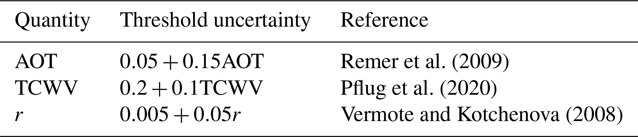
Land surface monitoring at optical wavelengths from medium resolution Earth observation (EO) requires an accurate and consistent description of the bottom-of-atmosphere (BOA) spectral bidirectional reflectance function (BRF) (Zhu et al., 2020) that is made readily available to users. This is acknowledged in efforts to develop consensus on “analysis-ready data” (ARD) (Wang et al., 2019; CEOS, 2019) and the value of such data for monitoring global change, as emphasised elsewhere (Feng et al., 2013; Hilker, 2018). Community needs for “CEOS Analysis Ready Data for Land” (CARD4L) (CEOS, 2020) are stated as “threshold” (minimum) and “target” (desirable) requirements, with the former reflecting current practice and what is achievable with existing approaches and the latter being an agreed position for the scientific and user communities to move towards. No uncertainty threshold or target values for surface reflectance are given in the CEOS ARD specification, but in this paper, we use specifications adopted by Doxani et al. (2022), given in Table 1, as threshold values for aerosol optical thickness (AOT), total column of water vapour (TCWV), and BOA BRF r specification.
Remer et al. (2009)Pflug et al. (2020)Vermote and Kotchenova (2008)Table 1Threshold uncertainty specifications for aerosol optical thickness (AOT), total column of water vapour (TCWV), and BOA BRF (r) used in this paper.
An important capability highlighted in target requirements is that per-pixel uncertainty estimates should be supplied (CEOS, 2021c), but this is lacking in the CEOS fully assessed USGS Landsat Collection 2 ARD product (CEOS, 2021a) and the ESA Sentinel-2 Level-2A (ESA, 2021b). Such information is vital for traceability and rigorous scientific analysis with ARD products (Merchant et al., 2017; Niro et al., 2021). Additionally, the ACIX intercomparisons of Doxani et al. (2018, 2022) and surface reflectance comparison studies (Flood, 2017; Nie et al., 2019; Chen and Zhu, 2021) illustrate that further work is needed to ensure accuracy and consistency of such data, which is critical for combining data with different spatial, spectral, temporal, and radiometric characteristics and for achieving more comprehensive and/or frequent monitoring than with any single set (Lewis et al., 2012b; Wulder et al., 2015). This requires a focus on both accuracy and inter-operability, which we suggest is not being adequately realised in current approaches.
In this paper, we describe the approach used for the UK NERC NCEO BOA BRF (https://catalogue.ceda.ac.uk/uuid/ad7de4e3b3b34cc0adca86c68e94d3a1, last access: 21 October 2022) product from medium resolution S2/MSI and L8/OLI sensors (NCEO, 2021). It is sensor agnostic over the optical domain in the sense that it does not rely on particular optical waveband sets, so is called Sensor Invariant Atmospheric Correction (SIAC). SIAC aims to be CARD4L-compliant at threshold requirements and to move towards target requirements by providing per-pixel uncertainty values. This is enabled by applying a Bayesian framework to the estimation of atmospheric parameters from medium resolution multispectral observations and other constraints. The resulting parameters are used to derive an estimation of BOA BRF. Mean estimates derived from SIAC are validated against the criteria in Table 1 through a global comparison of derived AOT and TCWV estimates with in situ AERONET measurements, comparisons of retrieved surface reflectance with in situ Radiometric Calibration Network (RadCalNet) measurements, and interoperability comparisons of surface reflectance between S2 and L8. The uncertainty in the retrievals is also assessed, which complements the further validation of SIAC and inter-comparison with other processors in the ACIX-II experiment (Doxani et al., 2022).
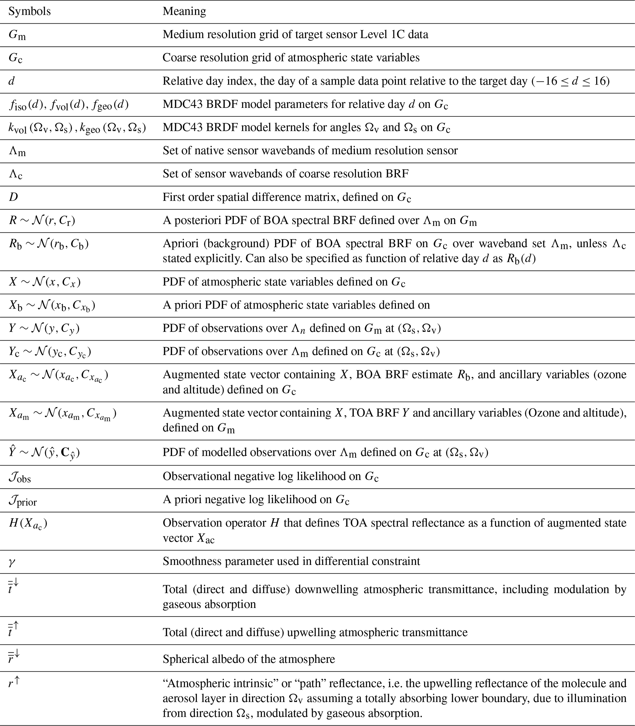
Table 2Main symbols used in the paper. C* represents the covariance matrix part of the PDF for parameter *.
2.1 Statement of the problem
We wish to estimate the probability distribution function (PDF) of BOA spectral BRF R with illumination and viewing vectors Ωs,Ωv, respectively, on a grid Gm of medium-resolution pixels over a set of wavebands Λm (see Table 2 for symbol definitions). Under these conditions, this is driven by medium-resolution observations Y from S2/MSI and L8/OLI sensors at 10–60 m resolution, in addition to other constraints. In SIAC, as in most other approaches, we first seek an estimate of atmospheric state X over the target scene. We assume multivariate Gaussian PDFs throughout and ignore non-linear impacts on transformed distributions. Our approach targets the maximum a posteriori (MAP) estimate, given an a priori estimate of X and Xb and the observations Y mapped to a grid Gc of coarse resolution pixels (nominal 500 m resolution). We then apply X at the original medium spatial resolution to the estimation of R on Gm. The heritage of the approach is the various works on Bayesian inference and optimal estimation applied to mapping atmospheric parameters from EO for other sensors (Tanré et al., 2011; Dubovik et al., 2011; Lewis et al., 2012b; Dubovik et al., 2014; Govaerts and Luffarelli, 2018; Kaminski et al., 2017; Lipponen et al., 2018; Hou et al., 2020), as this gives the framework for combining multiple sources of information and estimating per-pixel uncertainty. The MAP estimate of X over Gc is found by maximising the likelihood P(X|Y) (Rodgers, 2000):
with . The mean MAP estimate of X is achieved by minimising the negative logarithm of P(X|Y) in Eq. (1), i.e. the “cost function” 𝒥 with respect to X. X in the current version of SIAC contains AOT at 550 nm and total TCWV in g cm−2.
2.2 Overview
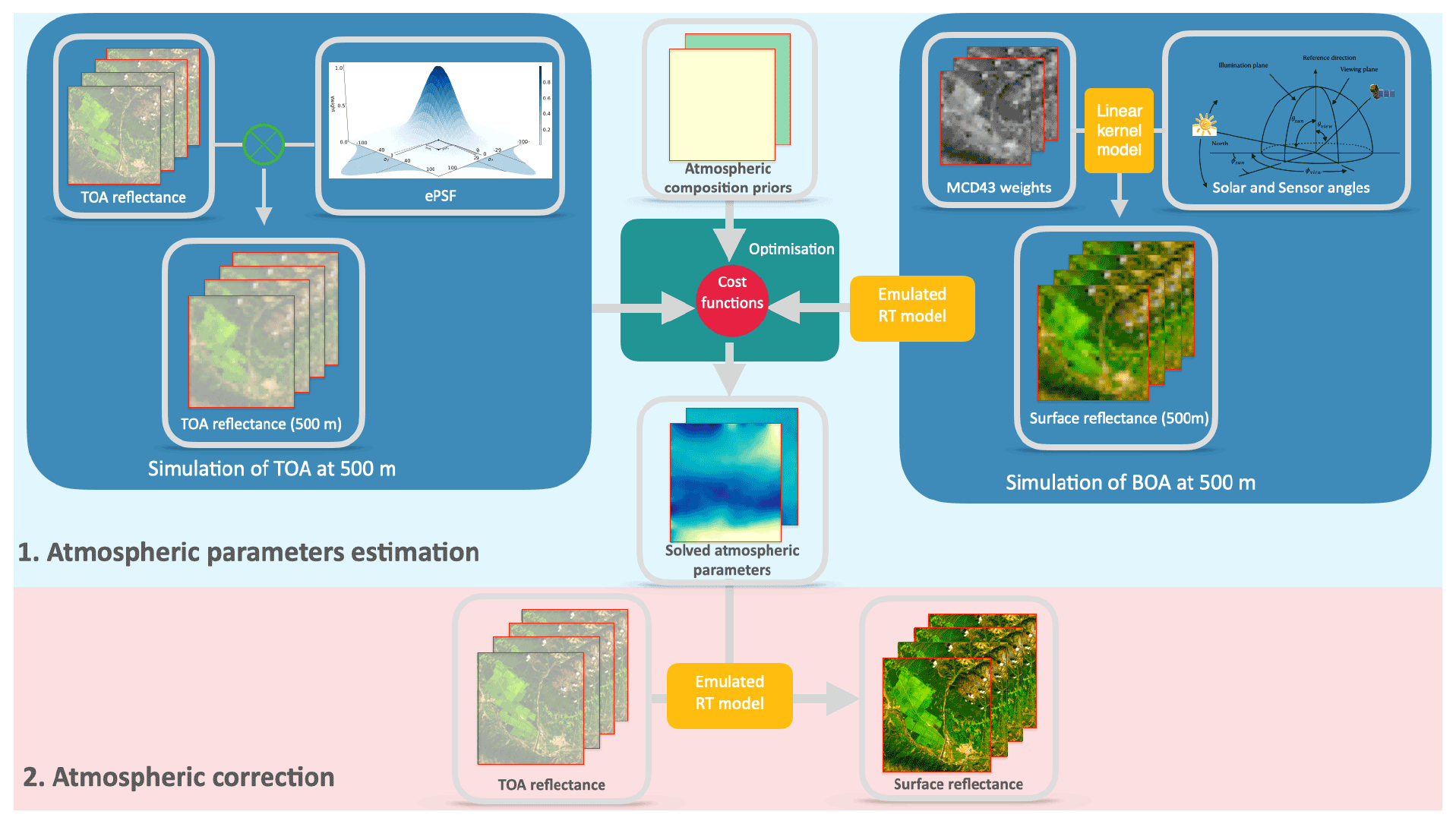
Our approach uses a priori constraints in the form of a coarse resolution (500 m) spectral BRDF dataset from MODIS (Schaaf and Wang, 2015) to provide sample land surface reflectance estimates as well as a very coarse resolution (40 km) estimate of atmospheric composition from the CAMS near-real-time (https://apps.ecmwf.int/datasets/data/macc-nrealtime/levtype=sfc/, last access: 21 October 2022) global assimilation and forecasting system (Morcrette et al., 2009; Benedetti et al., 2009), with an associated spatial correlation constraint for the atmospheric parameters. These are combined with observational data to solve an inverse problem to estimate atmospheric state at coarse resolution for the time and locations of the observations. We then use this to map from TOA to BOA reflectance (with associated uncertainty) at the native TOA data (S2 or L8) resolution. The method has the following steps, also summarised as a flowchart in Fig. 1. For the target observational dataset (S2 and L8, here) with given imaging location, geometry, and spectral bands, SIAC comprises two major steps:
- 1.
Atmospheric parameters estimation
- a.
Simulation of TOA reflectance Yc at 500 m resolution from observations Y, scaled with a calibrated MODIS effective point spread function (ePSF) model (Sect. 2.3.1);
- b.
Simulation of BOA reflectance Rb at 500 m from MODIS MCD43A1 product, mapped to target sensor spectral bands for sample pixels (Sect. 2.3.2);
- c.
Development of atmospheric composition prior estimates of AOT and TCWV in Xb from CAMS data, with a spatial correlation model on Xb (Sect. 2.4);
- d.
MAP estimate of the atmospheric parameters X given Yc, Rb, and Xb (Sect. 2.5).
- a.
- 2.
Atmospheric correction
- a.
Application of X to correct observed TOA reflectance Y to a posteriori estimate of BOA BRF R (Sect. 2.6).
- a.
In this paper, we present the theoretical underpinnings of the method and major results, relegating details of the implementation and additional results to the appendices.
2.3 Observational constraint
We can express the observational negative log likelihood as
Here, ⊤ is the matrix transpose operator and −1 the matrix inverse operator. Calculation of 𝒥obs as a function of variables in X requires confronting a set of observations yc with modelled estimates relative to the uncertainty in these, expressed as here. We derive these terms below.
2.3.1 TOA observations
The main data controlling the estimation of X (and so R) are medium-resolution observations Y of TOA spectral reflectance from S2 or L8 on a level 1C grid Gm used to form the observational constraint above over wavebands Λm (Table 3). A spectral mapping between MODIS and S2 and L8 is applied (see Appendix D) to correct the difference between their relative spectral response functions (hence the “sensor invariant” nature of SIAC). The output of the spectral mapping provides an estimate of reflectance from 400 to 2 400 nm every 1 nm. This provides a surface reflectance estimation for S2 B09, a band strongly sensitive to TCWV, even though MCD43 does not include this spectral region. Uncertainty from the spectral mapping is explicitly treated in the SIAC framework.
Table 3MODIS, S2, and L8 bands used in SIAC for the atmospheric parameters retrieval.
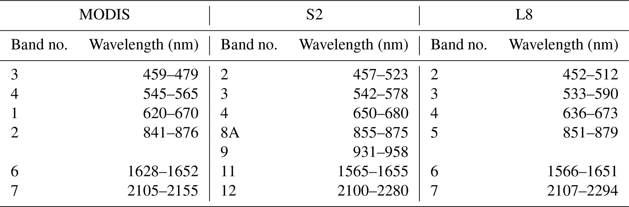
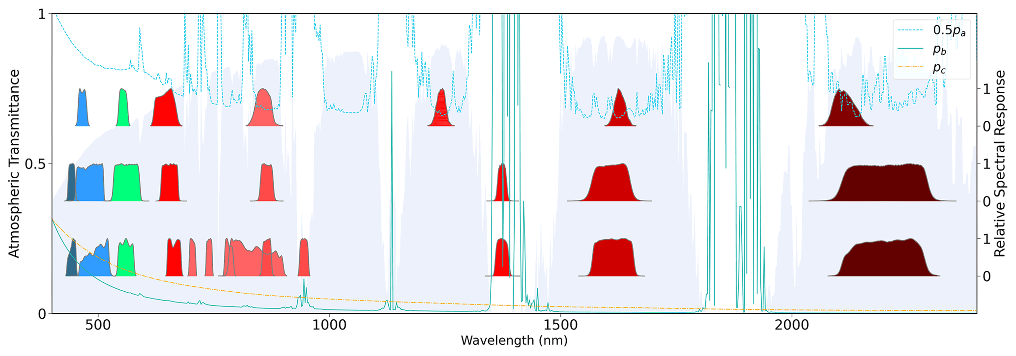
Figure 2From the top to bottom are the MODIS, L8, and S2 relative spectral response functions for each band, and the background is the atmospheric transmittance processed by 6S with US62 atmosphere profile and continental aerosol model with an AOT value of 0.2 at 550 nm.
We need TOA observational constraints Yc to drive Eq. (2). The atmospheric state X is defined at coarse resolution over grid Gc, so the observational likelihood term must also be defined at the same scale. This involves mapping valid observations from Y on grid Gm to coarse resolution equivalents Yc on grid Gc. This is achieved using the effective point spread function (ePSF) of the MODIS product following the approach of Mira et al. (2015), as described in Appendix E. The output through the ePSF modelling provides us with the TOA observations on grid Gc, i.e. MODIS grid. We ignore uncertainty associated with this aggregated reflectance in the estimation of X via Eq. (2), assuming it is small compared to the atmospheric model uncertainty (below).
2.3.2 Modelling TOA reflectance
We need an estimate of TOA reflectance given atmospheric state X to calculate 𝒥obs in Eq. (2), which is provided by a radiative transfer (RT) model. In this paper, we follow other current approaches to this for medium resolution data by assuming the surface is Lambertian and that each pixel can be treated as independent. Under these assumptions, is expressed by the “simple-form” relationship described for the 6S RT model by Vermote et al. (1997b):
where and , and is an augmented state vector, defined in Table 2, on grid Gc. The terms are lumped parameters for each waveband derived from 6 Sv (Vermote and Kotchenova, 2008). Clearly, pa≥1 and depends on pathlengths in the atmosphere. Outside of the strong absorption bands (L8 band 6, S2 bands B09, B11), it has a general pattern of decreasing with increasing wavelength, as illustrated in Fig. 2. The path reflectance normalised by transmittance, pb, and spherical albedo pc show a similar spectral trend and become small outside of visible wavelengths. pc impacts multiple scattering between the land surface and aerosol layer in the atmosphere and is manifested as a slight curve in the relationship between rb and y. Under the Lambertian assumption currently implemented in SIAC, these terms fully define the mapping from BOA BRF rb to TOA BRF as well as the inverse (estimating r from y). Within SIAC, they are calculated over a wide range of conditions using 6SV2.1. Running the model atmospheric model many times is computationally costly and is often approximated by using, e.g. look-up tables. Here, we provide fast surrogate approximations to the full atmospheric model – these are called emulators (Gómez-Dans et al., 2016). These approximations are based on fully connected artificial neural networks (ANNs) and provide an estimate of the pi terms as a function of the model inputs . Additionally, the Jacobian of the atmospheric model (needed for efficient gradient descent minimisation and for uncertainty propagation) is also approximated by the emulator, making use of backpropagation techniques (Hecht-Nielsen, 1992). In the current version of SIAC, we assume that atmospheric profiles used in 6S are from the US62 and that the aerosol type is “continental” (Vermote et al., 1997b). This choice of aerosol type may cause errors when conditions strongly depart from it, such as situations dominated by urban, maritime, or biomass burning conditions. See Tirelli et al. (2015) and Shen et al. (2019) for analysis of the impacts of aerosol types.
Direct calculation of TOA reflectance needs an estimate of rb for comparisons with observations y in Eq. (2). Many algorithms take a spectral approach to the problem, assuming that the ratio in TOA reflectance between visible and SWIR bands over dark dense vegetation (DDV) targets is constant (Vermote and Saleous, 2006; Kaufman et al., 1997; Vermote et al., 1997a; Remer et al., 2005; Levy et al., 2007b, a). Most operational algorithms for S2 and L8 are based on this, including LEDAPS for Landsat 4–7 (Masek et al., 2012), Sen2Cor for S2 (Louis et al., 2016), MAJA for S2 (Hagolle et al., 2015a), etc. However, this constraint can be of limited value if suitable DDV targets cannot be found well dispersed in the scene. Other relevant approaches applied to coarse resolution data find alternative methods to estimate surface reflectance: the Deep Blue method (Hsu et al., 2013) uses a coarse resolution seasonal global reflectance database for blue and red wavelengths over bright surfaces to extend the range of conditions that can be used; MAIAC (Lyapustin et al., 2018) develops an expectation from a time series of observations; and Guanter et al. (2007) use a set of spectral basis functions that need to be solved for each observational constraint sample. A variation of that is the use of a wider set of spectral basis functions used in processing hyperspectral data by Hou et al. (2020).
In SIAC, we avoid the sampling limitations of DDV and take advantage of these other ideas of providing a dynamic and globally applicable expectation of surface reflectance. We use the MODIS MCD43A1 BRDF/albedo (collection 6) product (Schaaf et al., 2002; Schaaf and Wang, 2015) to achieve this and derive an a priori model of surface reflectance for all target wavebands for the viewing and illumination angles Ωv, Ωs, respectively, of Yc. For relative day index d, this gives rb(d) at MODIS wavebands Λc, via the Ross-Thick Li-Sparse Reciprocal (RTLSR) linear kernel models (Wanner et al., 1997) and the values of the model parameters for relative day d:
Samples of this around the day of the observation d are used to provide a gap-filled, uncertainty-quantified estimate of rb(Λc), detailed in Appendix A. This is mapped to the target (S2/MSI or L8/OLI) waveband set Λm as rb(Λm), as given in Appendix D. The framework can tolerate incomplete coverage of , so we filter for plausible constraints from the MODIS data, as described in Appendix C, to avoid gross errors from inappropriate values of interpolated MODIS surface reflectance.
2.4 A priori constraint on atmospheric state
We can express the negative log of the prior pdf (up to a proportional constant) as
This gives a constraint based on a background (a priori) estimate of atmospheric state, Xb. In SIAC, the prior mean comes from the European Centre for Medium-Range Weather Forecasts (ECMWF) CAMS near -real-time (https://apps.ecmwf.int/datasets/data/macc-nrealtime/levtype=sfc/, last access: 21 October 2022) services (Morcrette et al., 2009; Benedetti et al., 2009) for estimates of atmospheric composition parameters AOT at 550 nm, total column water vapour, and total column of ozone in Xb and . These are at a coarse spatial resolution on a 40 km grid, but we need Xb on a 500 m grid to match with rb, so the data are interpolated to 500 m resolution.
The role of is to encode the prior expectation of variance and spatial correlation of the AOT and TCWV fields. AOT and TCWV variances are reported in the CAMS global validation report (see Sect. B2 for a detailed derivation).
We expect the AOT and TCWV fields to have long correlation lengths (Anderson et al., 2003), which result in non-zero off-diagonal elements in . This spatial correlation structure is defined using a Markov process covariance after Rodgers (2000). This has two free parameters: the variance and relative length scale. Since the covariance appears in the constraint Eq. (5) in inverse form, we use a fast approximation; this is derived from Rodgers (2000) and implemented as a first-order spatial difference constraint defined in matrix D.
Here, I is the identity matrix, k a normalising scale factor given in Eq. (B3), and γ an implicit function of the relative length scale that controls the degree of spatial smoothness. Numerical values used for uncertainty in SIAC are given in Appendix B.
The TOA reflectance observation, modelled TOA reflectance, and prior information on the atmospheric parameters are processed to Gc through the procedures described above. Thus, the D matrix is also defined at Gc, i.e. 500 m to provide spatial constraint for the atmospheric parameters. For a variable length of n, the matrix D is given as
Having this prior inverse covariance matrix allows a flow of information from regions in the scene that are well constrained by observations to areas that are poorly constrained or missing.
2.5 MAP estimate of X
We obtain the MAP estimate of x by minimising 𝒥 in Eq. (1) with respect to X. This is done simultaneously for all samples in the grid Gc of X using the efficient L-BFGS-B gradient descent algorithm (Byrd et al., 1995; Zhu et al., 1997). The approach and details follow Lewis et al. (2012a), using the derivatives of 𝒥 with respect to X. The cost function and its partial derivatives exploit the ability of the emulators to provide accurate approximations to the atmospheric RT model and its partial derivatives (Gómez-Dans et al., 2016). Multi-grid methods (following, e.g. Briggs et al., 2000) are used to iteratively provide spatially refined solutions. This greatly improves convergence rates in the optimisation over the large dimensional state vector of X. The uncertainty in X, Cx is calculated as in Appendix B3.
2.6 Atmospheric correction
We assume a Lambertian surface in the atmospheric correction process. The relative errors caused by this Lambertian assumption on the surface reflectance is 3 %–12 % in the visible bands and 0.7 %–5.0 % in the near-infrared bands. Its effect on the NDVI analysis is around 1 % and less than 1 % for albedo (Franch et al., 2013), which is within the 5 % accuracy requirement for albedo indicated by the Global Climate Observing System (GCOS) (GCOS, 2019). This Lambertian assumption is also widely used to produce the surface reflectance for MODIS (Franch et al., 2013), Landsat (Vermote et al., 2016), and S2 (ESA, 2021c), where the Landsat and S2 surface reflectance products have been accepted as the CEOS-assessed ARD products (CEOS, 2021b).
The mapping from Y to R given X at medium (10–60 m) spatial resolution on the grid Gm is achieved by rearranging the terms in Eq. (3) to give r (Vermote et al., 2006):
We calculate the with the mean atmospheric parameters x and the auxiliary data (Ozone and elevation) at MODIS spatial grid Gc. A linear interpolation is then used to re-sample the to the target sensor grid Gm, which is then used to derive the mean surface reflectance r with Eq. (8). The simple linear interpolation method used to resample the to sub-MODIS scale is justified, as atmospheric parameters are known to exhibit much larger correlation lengths (100s of km) (Anderson et al., 2003; Chatterjee et al., 2010). The TOA uncertainty is taken to be 5 % (Barsi et al., 2018b; Lamquin et al., 2019; MPC Team, 2021) for both S2 and L8 and is independent for each waveband. This is the threshold uncertainty value for S2 TOA reflectance. The calculation of per pixel uncertainty in r uses partial derivatives of r with respect to atmospheric parameters x and TOA reflectance y (Ku, 1966), as shown in Appendix B4. The per-pixel reflectance uncertainty derived in this way and propagated from uncertainty in the atmospheric parameters and the measurements is an important feature of SIAC.
2.7 Summary of SIAC approach
In SIAC, the atmospheric composition at 500 m is inferred by combining three sources of constraints:
-
an a priori constraint on land surface reflectance (at 500 m) derived from the MODIS MCD43 product
-
an a priori constraint on atmospheric composition (AOT and TCWV) derived from CAMS near-real-time predictions
-
an expectation of spatial smoothness (correlation) in atmospheric composition parameters at the 500 m scale.
The spatial and spectral mismatch between the original S2 or L8 products and MODIS are dealt with by modelling the MODIS ePSF (Appendix E) and using spectral mapping based on a hyperspectral data library (Appendix D), respectively. These constraints form the observational cost function 𝒥obs (Eq. 2 in Sect. 2.3) and prior cost function 𝒥prior (Eq. 5 in Sect. 2.4). By minimising the combined cost value (𝒥prior+𝒥obs), the uncertainty-quantified estimates of AOT and TCWV at the 500 m resolution are obtained. These estimates are then interpolated to the S2 or L8 spatial resolutions to parameterise Eq. (8) for the atmospheric correction.
ESA (2015)Roy et al. (2014)Tachikawa et al. (2011)ESA (2017)Schaaf et al. (2002); Schaaf and Wang (2015)Morcrette et al. (2009); Benedetti et al. (2009)Kokaly et al. (2017)Baldridge et al. (2009)Ilehag et al. (2019)Garrity and Bindraban (2004)Giles et al. (2019)AERONET (2021)Bouvet et al. (2019)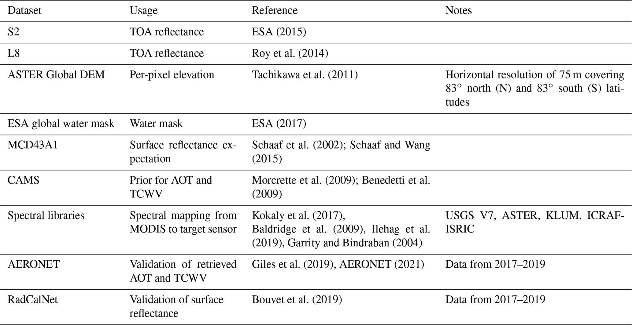
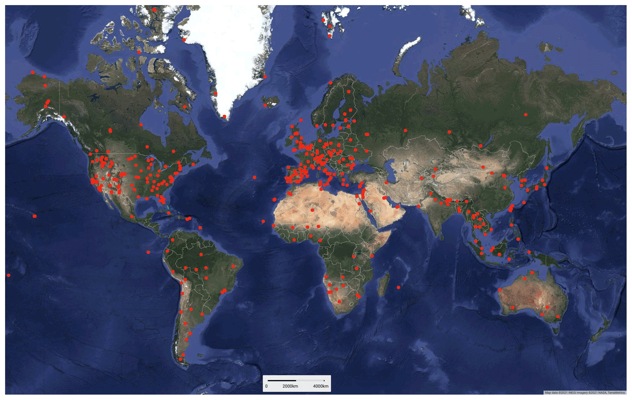
Figure 3Globally distributed AERONET sites (dot markers) used in this study for the validation of retrieved atmospheric parameters.
3.1 Study region and datasets
We validate using SIAC-derived atmospheric composition to estimate surface reflectance over globally representative sites for the years 2017–2019. We use S2 and L8 granules over more than 400 AERONET sites, seen in Fig. 3, as well as granules encompassing three RadCalNet sites (Railroad Valley Playa, La Crau, and Gobabeb sites). This gives more than 3 000 S2 tiles and more than 2 500 L8 tiles in the evaluation. The datasets used in this study, with comments on their use, are listed in Table 4.
3.2 AERONET
The AERONET (AErosol RObotic NETwork) (https://aeronet.gsfc.nasa.gov/, last access: 21 October 2022; Giles et al., 2019; AERONET, 2021) programme is a federation of ground-based remote sensing aerosol networks and provides globally distributed estimates of AOT, inversion products, and precipitable water. It has long been used as ground truth aerosol measurements and is used for the validation of various satellite inversions aerosol products. Atmospheric measurements from AERONET instruments were interpolated in time to get estimates corresponding to each satellite overpass. AOT at 550 nm was estimated using AERONET spectral log-transformed data with a second order polynomial between 400 and 860 nm following Kaufman (1993); Li et al. (2012). The measurement uncertainty of AOT from AERONET is taken to be 0.01 (Eck et al., 1999; Sayer et al., 2020), and that for TCWV is 0.15 % (Pérez-Ramírez et al., 2014).
3.3 RadCalNet data
The Working Group on Calibration and Validation (WGCV) of the Committee on Earth Observation Satellites (CEOS) has been providing ground surface reflectance data through the Radiometric Calibration Network portal RadCalNet (http://www.radcalnet.org, last access: 21 October 2022; Bouvet et al., 2019) since 2018, with measurements taken as earlier as 2013 in the US Railroad Playa Valley site. RadCalNet provides nadir-view, top-of-atmosphere reflectance at 30 min intervals from 09:00 a.m. to 03:00 p.m. local standard time at 10 nm intervals from 400 to 2 500 nm, which is calculated from ground nadir-view reflectance measurements and atmospheric measurements such as surface pressure, columnar water vapour, columnar ozone, aerosol optical depth, and the Angstrom coefficient. TOA reflectance is simulated by propagating the measured surface reflectance through the atmosphere using the MODTRAN radiative transfer model, parameterised by measured local atmospheric composition measurements.
Here, we compare the SIAC-corrected data with measurements from three RadCalNet sites: the ESA/CNES site in Gobabeb (Namibia), the CNES site in La Crau (France), and the University of Arizona's site at Railroad Playa Valley (Nevada, United States), as these three sites measure over the entire solar reflective spectrum. Railroad Playa Valley is a high-desert playa surrounded by mountains to the east and west; La Crau has a thin, pebbly soil with sparse vegetation cover; and Gobabeb is over gravel plains. The area of interest (AOI) of the radiometric measurements for the sites is taken to be 30 m×30 m for Gobabeb and La Crau but 1 km×1 km the Railroad Valley Playa. The appropriate (S2 or L8) sensor spectral response functions are applied to the RadCalNet hyperspectral measurements that are closest in time to the S2 and L8 acquisitions to derive RadCalNet estimates of BOA reflectance in S2 and L8 wavebands. Gross mismatches due to cloud or other artefacts (such as saturation of pixel value, cloud shadow, modelling error from the RadCalNet surface reflectance to TOA reflectance, etc.) are filtered by comparing RadCalNet TOA reflectance (provided by RadCalNet) estimates with S2 and L8 TOA reflectances; 5 % is used as the target uncertainty of the S2 and L8 TOA reflectance, and the RadCalNet TOA uncertainty is around 2 %–5 % for non-absorption bands (Wenny and Thome, 2022), which lead us to choose 10 % as the threshold to filter out bad samples. If the S2 and L8 TOA data fall outside a tolerance of 10 % of the RadCalNet TOA reflectances, we remove the sample from the comparison. This ends up with 273 S2 scenes and 72 L8 scenes over the RadCalNet sites, with 100 S2 scenes and 36 L8 scenes over Gobabeb, 93 S2 scenes and 19 L8 scenes over La Crau, and 80 S2 scenes and 17 L8 scenes over Railroad Valley Playa.
3.4 Sentinel 2 and Landsat 8
Sentinel 2A (S2A) and Sentinel 2B(S2B) were launched on 23 June 2015 and 7 March 2017, respectively. A single satellite revisits the Equator every 10 d, while a constellation of two satellites achieves an equatorial revisit time of 5 d, decreasing to 2–3 d at mid-latitudes. Each S2 has a 10, 20, and 60 m spatial resolution Multi-Spectral Instrument (MSI), with 13 spectral bands ranging from 443 to 2 190 nm. Identical to S2A and S2B, Sentinel 2C (S2C) is expected to be launched at the beginning of 2024, in which case S2A will be retired (ESA, 2021a).
The Landsat project has provided the longest temporal record of moderate resolution, multi-spectral data over the Earth's surface. Landsat 8 was launched on 11 February 2013, having a global revisit time of 16 d, with 8 d offset to Landsat 7 for 8 d repeated coverage. Two push-broom sensors – the Operational Land Imager (OLI) and the Thermal Infrared Sensor (TIRS) – are mounted on the platform to provide multi-spectral and thermal observations of the Earth's surface at 30 and 100 m resolution, respectively. OLI has nine spectral bands, among which band 8 is panchromatic and has a spatial resolution of 15 m. At the time of writing, Landsat 9 (Masek et al., 2020) had recently been launched (27 September 2021), but operational data are just coming online (USGS, 2021).
Both products provide projected and calibrated TOA reflectance datasets. Sentinel 2 products were obtained from the Copernicus Open Access Hub (https://scihub.copernicus.eu/, last access: 21 October 2022) and the L8 products from the USGS EarthExplorer (https://earthexplorer.usgs.gov, last access: 21 October 2022). The spectral characteristics of S2/MSI and L8/OLI, along with the MODIS land wavebands used in SIAC, are shown in Fig. 2 and Table 3.
We process all near-simultaneous (maximum 1 h apart) scenes and tiles from S2 and L8 over the years 2017 to 2019 over the AERONET sites illustrated in Fig. 3. This gives 2635 S2 and 1922 L8 scenes and 3472 point samples.
3.5 Validation approach and metrics
We want to evaluate how well SIAC estimates mean BOA BRF and associated uncertainty over S2 and L8 wavebands. We can validate mean reflectance against measurements for some conditions using RadCalNet data. However, we can also gain confidence in the results by validating interim products (atmospheric parameters), testing uncertainty via the discrepancy principle (Sayer et al., 2020), and examining patterns in uncertainty behaviour. Since we estimate surface reflectance from both S2 and L8 sensors and since these have some very similar wavebands, it is also worthwhile to look at the consistency of results between the sensors for samples over the same conditions.
We define residuals between values estimated from SIAC and measurements as follows:
for the residual for atmospheric parameters calculated from SIAC (xatm) and AERONET (xaeronet) and ΔRadCalNet for that between SIAC estimated reflectance and RadCalNet measurements rRadCalNet.
We define standardised residuals as follows:
where and are the uncertainty in the SIAC retrievals of atmospheric parameters and aeronet measurements, respectively (see Sect. 3.2). σr and are the uncertainty in the SIAC retrievals of surface reflectance and that of the RadCalNet measurements, respectively. Assuming Gaussian distributions, we would expect the mean of or ϵr to be 0 and the standard deviation to be 1 over a large number of samples. We follow Doxani et al. (2018) in calculating accuracy (A) and uncertainty (U) metrics against AERONET and RadCalNet observations through
where n is the total number of samples in a comparison, and Δ is or ΔRadCalNet, as appropriate. The related measure, precision (P), is given by . We recognise A as a measure of bias and U as the root mean squared error (RMSE). We assess SIAC against the threshold requirements in Table 1. For SIAC results to be within specification, we would expect 68 % to fall at or below the threshold value (assuming a Gaussian distribution) where samples or distributions are concerned. Where we calculate U, we would expect it to lie on or below the threshold value.
4.1 Validation of mean atmospheric composition over AERONET
We compare the 3 472 S2 and L8 samples over AERONET sites with independent in situ measurements of AOT and TCWV. Examples of the retrieved scene atmospheric parameters are given in Figs. F1–F3 in Appendix F. Since we use an a priori constraint on atmospheric state Xb in estimating X, we also assess Xb against the AERONET measurements to see what improvement the medium resolution observations offers in this context. Comparisons of CAMS and SIAC AOT with AERONET measurements are shown in Fig. 4, with more detail for A, P, and U (along with the number of samples used in each bin) given in Fig. 5. The threshold uncertainty (Table 1) is shown on the plots.
Over all AOT values (Fig. 4) for the a priori CAMS data, more than 73 % of samples are already within the threshold specification, which is slightly better than the 68 % expected. This increases to 77 % for S2 processing but is slightly reduced to 72 % for L8. The correlation coefficient is reasonably high for CAMS (0.58) but is dramatically improved by the data assimilation to 0.86 or better for S2 and L8. The regression for all cases is similar, with a slope that is slightly below unity (0.86–0.90) and a small intercept (0.03–0.05). The root mean squared error (RMSE, equivalent to the metric U over all samples) is moderately large at 0.169 for CAMS but is reduced to 0.071–0.076 by the assimilation. The A, P, and U plot shows that bias (A) is low and that uncertainty and precision are close to the expected error for low values of AOT for both sensors, with S2 mostly slightly better than L8. The results are more variable and sometimes out of specification for higher values of AOT, but the sample size is small for those cases.
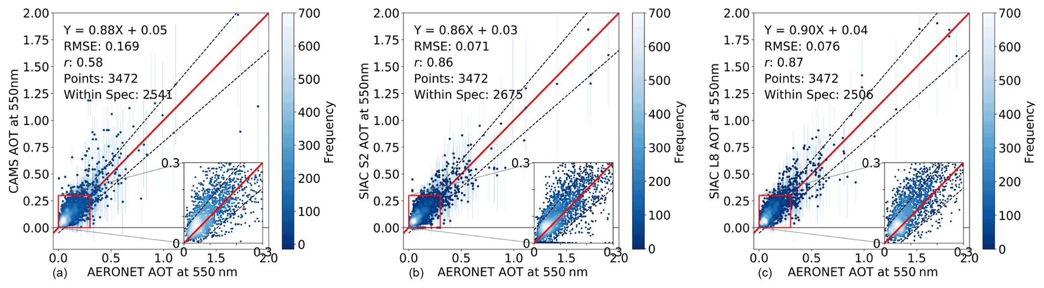
Figure 4AOT validation against AERONET measurements from CAMS (a), SIAC S2 (b), and SIAC L8 (c) over 3 466 matches, where the vertical lines of each point are the uncertainty of solved AOT values, and the horizontal error bars are AERONET measurement uncertainty of 0.01. On three panels, the inset plot shows the region marked by the red square in more detail, with . The threshold uncertainty is shown as black dashed lines in the figure.
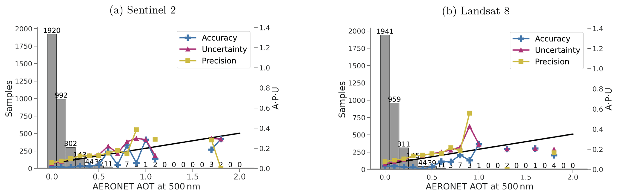
Figure 5The accuracy (A) (plus marker), precision (P) (square marker), and uncertainty (U) (triangle marker) validation of AOT against AERONET measurements. Threshold uncertainty is shown as black lines in the figure.
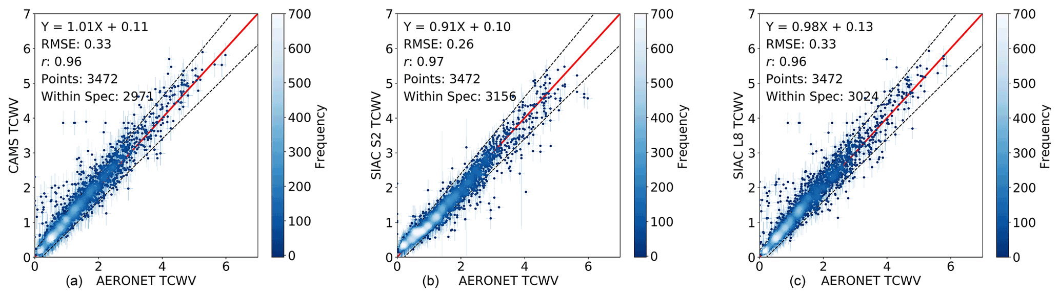
Figure 6TCWV (g cm−2) validation against AERONET measurements from CAMS (a), SIAC S2 (b), and SIAC L8 (c) over 3 466 matches, where the vertical lines of each point are the uncertainty of solved TCWV values, and the horizontal error bars are 15 % of AERONET TCWV values. Threshold uncertainty is shown as dashed lines in the figure.

Figure 7The accuracy (A) (plus marker), precision (P) (square marker), and uncertainty (U) (triangle marker) validation of TCWV against AERONET measurements. Threshold uncertainty is shown as black lines in the figure.
Comparisons of CAMS and SIAC TCWV with AERONET measurements are shown in Figs. 6 and 7. Over all values of TCVW, 86 % of the CAMS data are within specification. This is essentially the same after assimilation of L8 data but increases to 91 % for S2. The regressions for CAMS and L8 TCWV against AERONET have a slope close to unity and a low magnitude of intercept. The slope of the relationship is slightly poorer at 0.91 for S2. The A, P, and U plot shows that S2 results are within specification for the vast majority of values of TCWV, with poorer A and U only for the highest value and P slightly out of specification for the lowest value. For L8, the results are very similar to those from CAMS alone. In this case, all values are within expected error, other than the precision and uncertainty for low TCWV. In summary, the CAMS and L8 a priori data are very similar (very low impact of the observations), and the results are good for all but the lowest values of TCWV. The assimilation of S2 data (mainly from band B09) improves these lower values but seems to cause poorer result for the highest value of TCWV, though this may be because of the small sample number.
4.2 Consistency check for S2 and L8
The S2 and L8 scenes over AERONET sites described above were atmospherically corrected to surface reflectance using SIAC. Since the overpass times between sensors are within 1 h, we expect the surface reflectance in overlapping spectral regions from both sensors to be highly correlated and can use this to test consistency between sensors. Differences in spatial coverage, acquisition geometry, spectral sampling, and other sensor characteristics may impact this, but we will assume them to be small.
Pixels within a 2400×2400 m2 area around the AERONET sites in the S2 and L8 scenes presented above were considered for comparison. To account for geolocation errors and differences in spatial resolution, the L8 data were reprojected to the S2 reference system, and all data were spatially averaged to 60 m resolution. A filtering for cloud, shadow, and any large changes between scene acquisitions was then applied. Rather than relying on the cloud or shadow masks for this, we use compatibility in TOA reflectance to select candidate pixels. According to studies (Gascon et al., 2017; Barsi et al., 2018a; Helder et al., 2018; Pahlevan et al., 2019; Lamquin et al., 2019) and operational validation reports (Clerc and MPC Team, 2021), the agreement of nearby spectral bands (Table 3) should be better than 5 %. Since we allow a larger temporal gap between S2 and L8 than some of these studies (1 h), we use a filter on a threshold of 10 %+0.01 between S2 and L8 TOA reflectance. This leaves around 3×106 pixels for comparison.
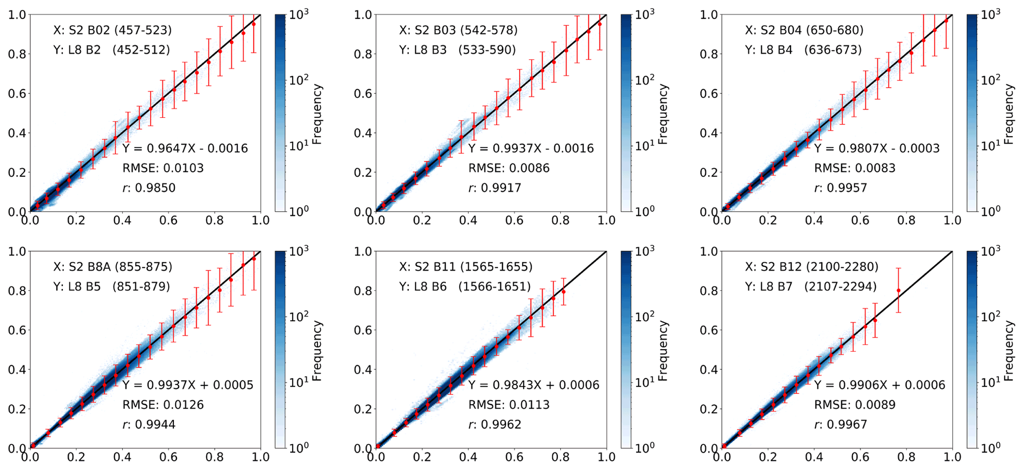
Figure 82D histogram of surface reflectance after the atmospheric correction from 3 466 S2 and L8 near simultaneous observations; each subplots shows the results for the closest S2 and L8 bands. The colour bar is shown using a logarithmic scale. The error bars are 3σ of the difference between the S2 and L8 corrected reflectance, which is computed at an interval of 0.05 from 0–1.
The results are shown in Fig. 8 as a set of two-dimensional histograms. The reflectances are highly correlated (coefficient of determination r>0.98 for all bands and r>0.99 for bands in the NIR and SWIR regions), with a small RMSE (RMSE<0.012). The bias is very small (less than 0.0016 for all bands), and the slope is between 0.96 (blue band) and 1 (NIR band). The error bars of S2 and L8 bands are slightly larger than the 10 % +0.01 used to filter the TOA reflectances. This slight increase in the difference between S2 and L8 surface reflectance comes from the increase in uncertainty during the atmospheric correction process, but this is any case small.
4.3 Validation of uncertainty in atmospheric parameters
We need to verify that uncertainty values σx calculated by SIAC are useful in characterising actual uncertainty. We approach this using the “discrepancy analysis” method suggested by Sayer et al. (2020) to check if the error distributions in the AERONET comparisons described above follow an expected distribution. We calculate standardised residuals following Eq. (11) for AOT and TCWV for each sample. We know that different configurations, data, and algorithmic effects mean that some retrievals will be more accurate than others, so here, we test our ability to identify this by weighting the departure of SIAC estimates from AERONET measurements. If we have grossly overestimated uncertainty relative to actual discrepancy, then the standard deviation of the standardised residuals will be much less than one and vice-versa if we underestimate. A limitation of the assessment is that it can only be calculated over the AERONET sites where an independent measurement is available. But still, if the results mainly follow the expected statistics, it shows that the magnitude of uncertainties calculated in SIAC are plausible.
Part of the a priori constraint in SIAC is the imposition of a degree of smoothness on the atmospheric parameters through the parameter γ in the inverse covariance function in Eq. (6). We use γ values of 5 for S2 and L8 AOT, 5 for S2 TCWV, and 0.1 for L8 TCWV in SIAC. Cross-validation studies suggest that there is a wide range of suitable values for γ (Appendix G for additional details on this choice and its implications). The scaling term k in Eq. (6) should mean that the magnitude of uncertainty is not greatly affected by γ. But since many applications of this type of constraint (Dubovik et al., 2011; Lewis et al., 2012a; Govaerts and Luffarelli, 2018) do not explicitly apply such a normalisation, we test the impact of that here and examine the distribution of over a range of γ values in Figs. 9 and 10.

Figure 9Standardised residual distributions for S2 AOT (a) and L8 AOT (b) with γ of [0.001, 0.1, 1, 5, 10, 100, 1000]. The red histogram distributions show standardised error distributions (Error distribution) from the data and the blue ones the estimated Gaussian distribution from the distributions (Fitted Gaussian).
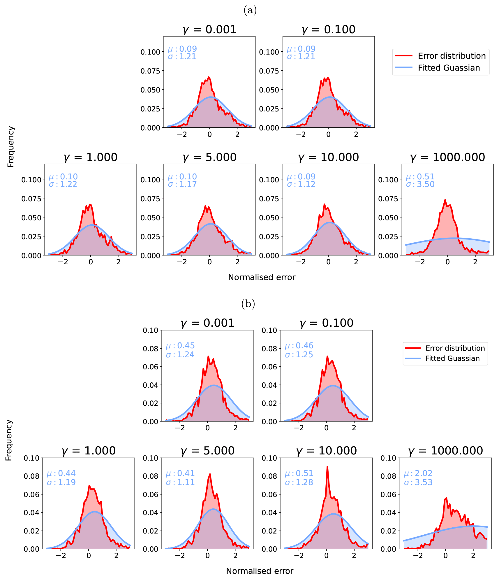
Figure 10Standardised residual distributions for S2 TCWV (a) and L8 TCWV (b) with γ of [0.001, 0.1, 1, 5, 10, 100, 1000]. The red histogram distributions show standardised error distributions (Error distribution) from the data and the blue ones the estimated Gaussian distribution from the distributions (Fitted Gaussian).
The results show that, for γ<10, the standardised residual distributions of AOT for S2 and L8 remain broadly similar, i.e. the normalisation using k seems to be effective. For S2, there is a small positive bias in AOT that decreases with increasing γ, but the standard deviation σ is around 1.0. For L8 AOT, there is a small positive bias in all cases (larger than for S2), but σ is close to 1. Above γ=10 for both, σ increases and becomes unrealistic for very high γ, so the normalisation is ineffective for extremely high values, possibly relating to boundary condition effects on Eq. (6) as an approximation to the intended inverse Markov process covariance function.
The distributions of for S2 TCWV retrieval show a slight overestimation in the TCWV uncertainty (σ smaller than 1) but almost no bias for γ<10. The L8 retrieval for TCWV is mainly controlled by the prior information, and the normalised error is close to 1, but with a broader distribution compared to S2 TCWV, as no water absorption band is available from L8 measurements. Again, the behaviour of these distributions for TCWV broadly confirms our choice of γ for S2, but it seems that a higher value for L8 might be tolerated, and a compromise value of 5 might reasonably be used for γ for all terms.
4.4 Validation of mean surface reflectance
We validate mean SIAC reflectance by comparison with ground measurements over RadCalNet sites. We compare mean S2 and L8 BOA reflectances from SIAC averaged over defined RadCalNet AOI boundaries with the RadCalNet estimates of BOA reflectance in Figs. 11, 12, and 13. Since TOA reflectance estimates are provided for the RadCalNet sites using observed surface reflectance and atmospheric parameters calculated with the 6S model, we also compare measured TOA reflectance for S2 and L8 with these. This provides context to interpret both the spectral signatures and any biases or other issues in the data. If there are mismatches between the TOA datasets (e.g. from sensor calibration), since one is essentially a direct (S2 or L8) measurement and the other developed only with measurements from the RadCalNet sites, we would not expect to do better than that using SIAC, where we have to estimate the atmospheric parameters.
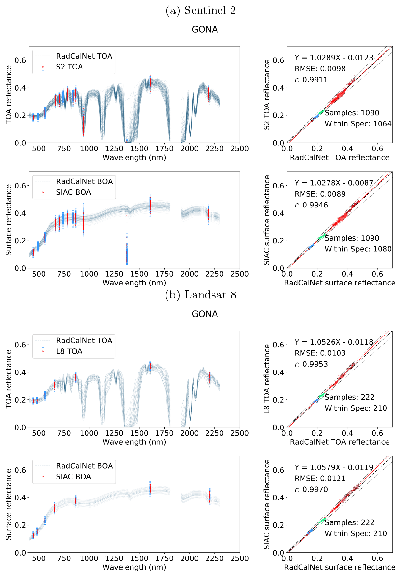
Figure 11Comparison between the S2 (a) and L8 (b) TOA reflectance and RadCalNet simulated nadir-view TOA reflectance (top row), and the surface reflectance after correction against RadCalNet nadir-view surface reflectance (bottom row) at Gobabeb. The blue lines on the left are different spectra measurements from RadCalNet, and the red dot with blue error bars (1 standard deviation) are the TOA or surface and TOA reflectance with uncertainty. The EE is defined as , denoted as black dashed lines in the scatter plots. The regression line is draw as a red line and the 1-to-1 reference line is drawn as a thick black dashed line in the middle.

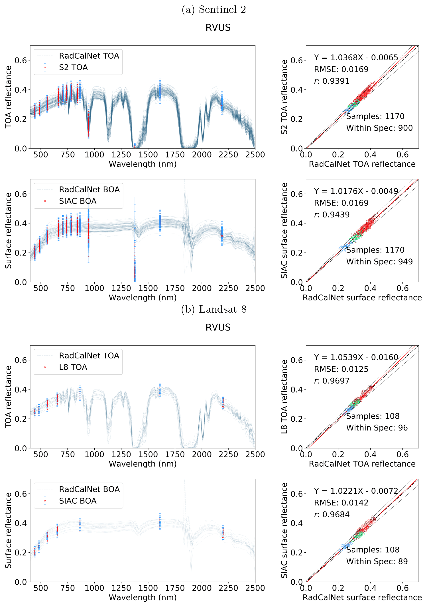
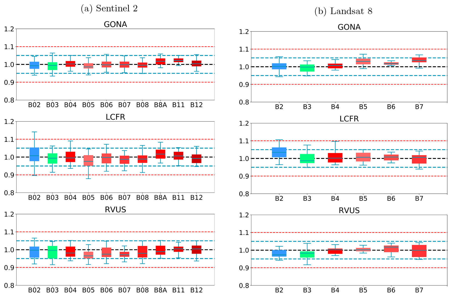
Figure 14The ratio of SIAC-corrected S2 (a)and L8 (b) surface reflectance to RadCalNet surface reflectance over three sites. The black dashed line in the middle is the reference line of ratio 1, indicating the same values of SIAC-corrected S2 (a) and L8 (b) surface reflectance and RadCalNet surface reflectance. Values above the reference line indicate positive bias (SIAC overestimates compared to RadCalNet) and below it indicate negative bias; 5 % and 10 % biases are shown as dashed lines. Boxplot colours are the same as colours in Fig. 2
The agreement between the SIAC-retrieved surface reflectance and the reference measurements is very strong for all sites, with RMSEs values for the BOA products of around 3 %–5 % of RadCalNet ground measurement reflectance over all wavebands. The correlation coefficient r is very high (>0.94) for all cases and is seen to increase slightly between TOA and BOA reflectance. The proportion of samples within the specification for TOA reflectance and SIAC-corrected surface reflectance are very similar. For BOA, there is 98 % for S2 and 95 %, respectively, within the specification for L8 over Gobabeb site, 88 % for S2 and 87 % for L8 over La Crau site, and 77 % for S2 and 86 % for L8 over Railroad Playa Valley site, so the results overall are well within the specification. Most samples outside of this can be attributed to the TOA reflectance being outside the RadCalNet TOA expectation limits. The patterns in the scatterplot of the small apparent biases in BOA reflectance are mirrored in the TOA analysis, suggesting that these arise from factors extraneous to the atmospheric correction. Interestingly, the results obtained using only the a priori CAMS data (included in Appendix I) show almost the same performance compared to RadCalNet as mean SIAC reflectance retrievals. The fact that sometimes the BOA statistics are better than the TOA is probably due to the better dynamic range of the surface reflectance signal compared to the TOA one.
The best performance is found over Gobabeb, but the results are only slightly poorer for La Crau, which has more variation in the pattern of spectral reflectance. The broader spread of results for the BOA analysis for Railroad Playa Valley is mimicked in the TOA data. A per-band analysis of the ratio of SIAC BOA reflectance to measured ground data over each RadCalNet site is given in Fig. 14. For Gobabeb, most of the time, the SIAC surface reflectance is within 5 % of RadCalNet ground measurements for all S2 and L8 bands, excluding the water absorption and Deep Blue bands (not shown). A similar situation is observed for the other two sites – although the distributions overrun the 0.95 mark at times, they are always within 10 %. The interquartile range (IQR) (McGill et al., 1978) is within the 5 % limit in all cases other than L8 B2, where it goes slightly above.
4.5 Validation of uncertainty in surface reflectance
Although the assessment of σx presented above is useful in understanding SIAC performance, we are ultimately more interested in knowing whether BOA reflectance uncertainty values σr calculated by SIAC are useful in characterising surface reflectance uncertainty. We can do this with the same approach as above, calculating the standardised residual ϵr from Eq. (12) between SIAC reflectance averaged over the RadCalNet AOIs and the RadCalNet measured reflectance convolved with the appropriate S2 or L8 bands. The expectations for this from the discrepancy principle are the same as for , as described above. Figure 15 shows the distributions of ϵr for the main surface reflectance wavebands.

Figure 15SIAC surface reflectance uncertainty validation. The red histogram distributions show standardised error distributions (Error distribution) from the data and the blue ones the estimated Gaussian distribution from the distributions (Fitted Gaussian).
The histograms are quite noisy, particularly for L8, suggesting that the results might be impacted by a low sample number. For S2, the mean is very close to 0 for around half of the bands but can show a positive bias of up to 0.54 (B11). The standard deviation σ is less than 1 for all cases, being as low as 0.73 for B11, indicating that we are likely overestimating the surface reflectance uncertainty by a factor of between 1.04 (B12) and 1.37 (B11) for S2. The L8 analysis shows broadly similar results, with a positive bias in the mean of similar magnitude. However, the values of σ are generally lower, ranging from 0.55 (B06) to 0.75 (B07), suggesting an overestimation of uncertainty by a factor of between 1.33 and 1.8. In summary, our tests show that we have a conservative estimate of uncertainty. The overestimation of the variance in surface reflectance is more marked for L8 than S2.
4.6 Surface reflectance uncertainty behaviour
The work of Hagolle et al. (2015b) showed that there are patterns to be expected in plots of uncertainty as a function of surface reflectance. The TOA uncertainty is assumed to be σy=0.05y. Combining the ideas from Hagolle et al. (2015b) and an examination of the equations from this paper, it is possible to gain further insights into the factors controlling the uncertainty in surface reflectance and to confirm that SIAC estimates of uncertainty follow the patterns as expected.
For low AOT and longer wavelengths, the sensitivity to uncertainty in AOT is low, and the term Δyσy will mostly dominate. For these conditions, pb and pc will be very small (see Fig. 2), so Δy≈pa from Eq. (B8), so , and Δyσy≈0.05r. For shorter wavelengths, sensitivity to uncertainty in AOT increases. So, even for low AOT, the uncertainty is expected to be more than 0.05r. For higher AOT and TCWV, there is significantly higher sensitivity to uncertainty in atmospheric parameters. In this case, uncertainty should have behaviour similar to Fig. 1 in Hagolle et al. (2015b), with a critical value of r, for which in Eq. (B7) is 0. For values of r less than or greater than the critical value, the contribution from uncertainty in atmospheric parameters increases, resulting in a “V”-shaped behaviour if σr is plotted as a function of r. Figure 16 shows scatterplots of typical behaviour of this. These are plotted for full S2 scenes for an example of a low AOT case (mean 0.15, ranging from 0.02 to 0.35) and high AOT case (mean 1.1, ranging from 0.9 to 1.25). Results are shown for each waveband, with the colour corresponding to those used in Fig. 2. The turning point reflectance for each band is indicated by a dashed line in that colour.
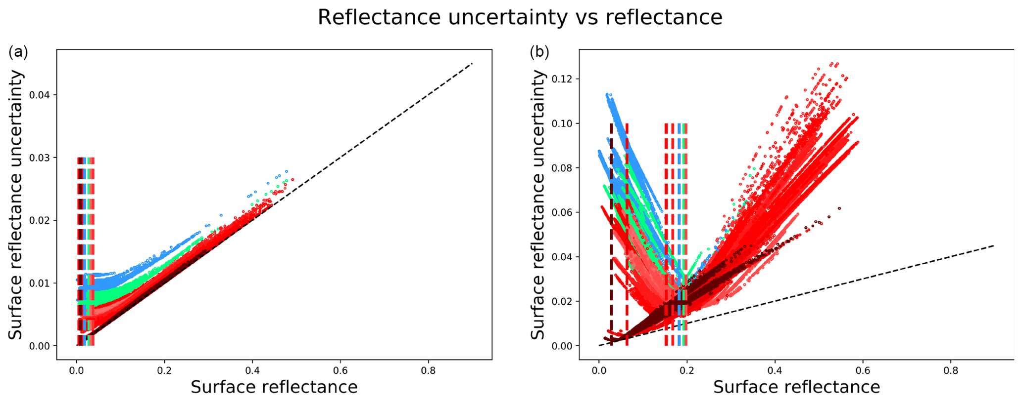
Figure 16SIAC S2 uncertainty for different bands for low AOT (a) and high AOT (b). The baseline 5 % is noted as a dashed black line, and the minimum of the uncertainty of each band is noted with coloured dashed lines. Colours are used to indicate the bands shown in Fig. 2.
The turning point feature mainly arises from the AOT component of uncertainty in equation Eq. (B9). We have seen that uncertainty in AOT is expected to be higher for higher AOT (Fig. 5); so for lower AOT, this component will be of lower magnitude, and the uncertainty will be dominated by TOA reflectance uncertainty. For higher AOT, the AOT uncertainty becomes more significant, especially for visible wavebands, and this feature becomes a more dominant part of the uncertainty behaviour, as we would expect.
The black dashed line in the subplots shows the lower boundary of 5 % uncertainty that would be expected for a TOA uncertainty of 5 %. All values appear on or above this line, providing some confidence in the calculations within SIAC. For low AOT, the longer the wavelength, the closer the behaviour directly mimics the TOA relative uncertainty. This arises from the decreasing magnitude of pb and pc with wavelength, as seen in Fig. 2. As these terms become negligible, the TOA and BOA reflectances become more proportionately related, and so with TOA reflectance uncertainty (low AOT), the proportionate TOA uncertainty more closely maps to proportionate BOA uncertainty.
5.1 Contributions of SIAC
Current approaches to atmospheric correction of S2 and L8 data over land use readily available and well-tested atmospheric RT codes, such as 6S, considered adequate for the task at hand (Vermote and Kotchenova, 2008). Since BRDF effects are not well sampled, they use the “simple form” of radiative interaction in Eqs. (3) and (8), allowed by assuming the surface Lambertian. For the most part, they proceed by applying some sort of mask for clouds or other extraneous features, estimating atmospheric state X based in part on observational constraints, and applying X to estimate surface reflectance r via Eq. (8). As we have noted, they do not currently estimate per-pixel uncertainty. Differences in performance between approaches seen in exercises such as the ACIX intercomparisons of Doxani et al. (2018, 2022) then come as a result of how effective the masks are and how they estimate X. We do not attempt to explore the first of these issues in this paper. Issues in the latter can come down to the validity of assumptions that are made but can also be very dependent on getting a suitable spatial distribution of observational constraints.
SIAC follows these same steps and broad assumptions, but a major feature of the approach is its use of the reliable external operational data streams available nowadays in support of its estimations. It has other novel features, including accounting for PSF impacts in the scaling from L8 and S2 to MODIS. It is further distinguished by applying a Bayesian framework that is able to weigh up these contributions according to their uncertainty and directly estimate the resultant uncertainty in X, from there providing a per-pixel estimate of uncertainty in r. It is a data assimilation approach.
Rather than the more limited extent available for DDV approaches, SIAC uses a direct expectation of surface reflectance from an external coarse resolution source (MCD43), meaning that the keystone observational constraints can supply information to the solution over a wide range of conditions. This means that the solution is, to some extent, reliant on the accuracy of these MODIS reflectance predictions, so we go to some lengths to filter out samples that may not be reliable predictors. In this first implementation of SIAC, we ignore snow and water pixels as well as some other conditions (Appendix C), which may be over-cautious. The estimate of X in SIAC is based on multiple constraint, so it is not in any case entirely dependent on the presence or quality of the observational constraints. The entire process (this includes state estimation, surface reflectance estimation, cloud masking, and uncertainty quantification) of a single S2 or L8 scene on a standard workstation with a 3.1 GHz i7 CPU and 16 Gb RAM takes between 20–30 min on a single process.
5.2 Accuracy assessment
SIAC aims to be CARD4L compliant and to meet threshold requirements for uncertainty. Validation results show that the method gives accurate (within threshold specifications) retrievals of uncertainty-quantified land surface reflectance, both for S2 and L8, for the most part. Moreover, the surface reflectances for the two sensors are compatible, an important step in using these sensors together for land monitoring applications.
A data assimilation system relies on having well-quantified uncertainties on the constraints used. This is vital in a relative sense for balancing contributions from different sources but also in an absolute sense for quantifying uncertainty. Unfortunately, none of the constraints we use have a per-pixel estimate of uncertainty to drive the analyses, so instead (Appendix B) we provide reasonable estimates, with references to justify the choice of uncertainty parameters and to assess the performance of the uncertainty estimates as part of the validation. In the absence of much observational constraint in a scene or area of a scene, our solution is based mainly on CAMS, so it should still provide a good, though less well spatialised, result. We see this to be borne out in the validation results for AOT and TCWV in Figs. 4 and 6: a small additional percentage of AERONET samples come within specification in SIAC compared with the CAMS data, and the regressions equations remain very similar. What SIAC achieves is a large increase in the correlation coefficient for AOT and a reduction in RMSE, suggesting that this localisation is being achieved. When these results are analysed as a function of AOT, the bias A is seen to be very low for AOT up to 0.5 (all comparisons that have more than 11 samples), with U and P lying almost exactly on specification. It is difficult to draw conclusions for AOT values beyond this due to the small sample size. There is some evidence that AOT uncertainty is slightly higher for L8 than for S2. For TCWV, the RMSE for S2 improves over that of CAMS, though it remains the same for L8. For S2, for all comparisons with more than 12 samples, P and U are well within specification, but for L8, this is not the case for TCWV values of less than around 1 g cm−2.
The validation of atmospheric parameter uncertainty in Sect. 4.3 suggests that the uncertainties calculated in SIAC are plausible for the selected values of γ according to the discrepancy principle (Sayer et al., 2020). Additionally, we have confirmed that the uncertainty estimation from SIAC is not strongly affected by the choice of γ.
The results of comparison between SIAC BOA reflectance and RadCalNet measurements (Sect. 4.4) suggest that the atmospheric correction is comparable to the atmospheric modelling done with the RadCalNet data driven by observed atmospheric parameters. The number of samples within specification is much higher than expected at the threshold assumed. For most land surface bands and most sites, relative errors are within 5 %.
Most of the time, at least over the conditions represented by RadCalNet, we can expect SIAC to estimate surface reflectance r within the threshold specification. Further, the surface reflectances from S2 and L8 are seen to be consistent: the processing has not created artificial biases between the surface reflectance from the two sensors, a feature seen in several papers on the comparison of S2 and L8 surface reflectance (Li et al., 2018; Runge and Grosse, 2019). With the assumed 5 % TOA uncertainty, SIAC overestimates surface reflectance uncertainty, as shown in Sect. 4.5. This suggests that we might reasonably relax the assumption of 5 % uncertainty in TOA reflectance for S2 and L8 towards a 3 % value (other than B12) that would be consistent with Lamquin et al. (2018, 2019). The result for L8 is similar to that for S2 but with estimated maximum TOA uncertainty of around 2.5 % from this analysis. The calibration of TOA uncertainty is detailed in Appendix H.
Surface reflectances produced by SIAC are of high accuracy and are consistent for S2 and L8, as shown in Sect. 4.4 and 4.5. But we also find that atmospheric correction results derived solely from CAMS atmospheric information over the RadCalNet sites demonstrated similar average behaviour (Figs. I1, I2, and I3 in Appendix I). The main impact of the assimilation of observational data is a reduction in uncertainty of 10 % for S2 visible to near-infrared bands and 5 % for S2 SWIR bands with the assumed TOA uncertainty of 3 %–5 %. This is because the TOA uncertainty dominates the total uncertainty budget in the surface reflectance when the AOT is low (mean AOT is around 0.08 over RadCalNet sites). However, we should bear in mind that these sites are not necessarily representative of the challenging environments that might be encountered in global processing. The RadCalNet sites are located in places with quite homogeneous landscapes and mostly low aerosol loading (RadCalNet, 2018b), which is probably the main reason why there seems to be little improvement in mean reflectance after assimilation. This suggests that RadCalNet measurements should be used as a minimum test of any atmospheric correction method rather than a solid evaluation of the accuracy of atmospheric correction, and we ideally need more measurements covering different landscapes with variations of atmospheric states.
5.3 Future developments
In this paper, the atmospheric composition is set by a model (6S in this case) and by a choice of aerosol optical properties (continental aerosol model). The use of emulators of the RT model makes it easy to change the RT model entirely in the code or to use a different configuration of the model used. We can also extend the scheme to retrieve independent aerosol species concentrations by both modifying the RT model (and thus extending the number of parameters that go in the inference) and by using data on species distribution available from CAMS and extending the prior to cover these. A similar approach has been implemented in the MAJA processor (Rouquié et al., 2017), which uses the CAMS aerosol species data to define the aerosol types for the atmospheric correction and has found improved atmospheric correction results over deserts. This approach may well be valuable in areas of high dust aerosol loading or in situations where biomass burning results in an important contribution to aerosol concentrations.
SIAC relies on the surface reflectance constraint from the MODIS MCD43 product, but the current MODIS satellites are approaching the end of their mission (Skakun et al., 2018; Xiong and Butler, 2020). VIIRS is designed to produce a continuity data record to MODIS, so it may be possible to use the VIIRS VNP43 product (Justice et al., 2013) as an alternative surface constraint, but this has not been tested. VIIRS land products additionally include bands within the Deep Blue spectral region (M1, M2), which are more sensitive to the aerosol variation. This information may be used to constrain the S2 and L8 Deep Blue bands to retrieve AOT over bright surfaces (Hsu et al., 2013).
We need an estimate of BOA BRF at Λm, which we derive from an estimate of BOA reflectance Rb(Λc) from the MDC43 products. But the observation on the target day may be missing or of low quality. We seek to replace this with a gap-filled estimate based on the product QA flags. Gap filling is achieved with a robust smoother (Garcia, 2010), having a smoothing factor s of 0.5 (low smoothness). The inverse of bi-square weight W for the target date, given by Garcia (2010), is used to scale relative interpolation uncertainty. Then for each of the six bands in Table 3 is given by:
where the base-level uncertainty of 0.015 is the broadband uncertainty in QA =0 retrievals assessed by Wang et al. (2018); the spectral weighting follows Guanter et al. (2007) and is applied to give a conservative estimate of uncertainty in the prediction of Rb(Λc) and to weight lower wavelengths more strongly. Here, is the value of for band index i, with centre wavelength Λi.
A data assimilation system combines evidence from different streams by weighting them by their inverse uncertainties. In SIAC, the statistics of the uncertainties are assumed to be zero-mean Gaussian and thus only characterised by an associated covariance matrix. We review here the sources and values of these uncertainties. The observational and a priori constraints for the estimation of X contain inverse covariance matrices and that need definition. We also need to define the uncertainty associated with a posteriori BOA BRF R, Cr.
B1 Observational uncertainty
The observational uncertainty in Eq. (2) has three main components that we can call Cm, CΛ, and CG. The uncertainty associated with the MODIS BRF predictions arises mainly from (i) uncertainty in the MODIS BRF predictions and the temporal interpolation strategy, and (ii) the spectral transformations. The uncertainty in rb(Λc) is given as in Sect. 2.3.2. The uncertainty from the spectral transformations CΛ is calculated as the RMSE following Appendix D. The observational uncertainty of the L1C product convolved with estimated ePSF, , is assumed to be much smaller than and is ignored in the estimation of X. Any other uncertainties arising from the inadequacy of the radiative transfer model are also ignored. We assume to be a diagonal matrix, so we need only define the variance terms .
Following Guanter et al. (2007), we apply an additional spectral weighting over relative wavelength , where is the mean of central wavelengths of the target sensor in Λm over all bands raised to the power of −1.6. This has the effect of giving higher weight to shorter wavelengths to emphasise sensitivity to AOT. is taken as a diagonal matrix, with elements
for each waveband in Λm, defined on Gc.
B2 A priori state uncertainty
We take the CAMS estimates of atmospheric state at 40 km × 40 km to be the mean values in xb. Schulz et al. (2020) report that, globally, AOT has a small bias (−0.04) and an RMSE between forecast and observation of 0.17 versus AERONET match ups. Zhang et al. (2020) report higher values around 0.23 over China, which suggests that we should take a more conservative approach in defining the uncertainty; so in SIAC, the a priori standard deviation for AOT is a function of AOT, with a minimum threshold. A similar process of comparing CAMS TCWV with AERONET matchups is used to arrive at a relative uncertainty of 0.3 for TCWV. in Eq. (5) is assumed to be a diagonal matrix. We first define standard deviation terms for the variables in X:
where xb(aot) and xb(tcwv) are the a priori estimates of atmospheric state in Xb on Gc. We assume no correlation between uncertainty in AOT and TCWV.
The inverse covariance function given in Eq. (6) is parameterised by smoothness γ and is applied on the grid Gc, with the first difference operator D applied across rows and columns1. The normalisation factor k2 is the mean eigenvalue for , which can be given as (Garcia, 2010)
where n is the number of rows (columns) of pixels within the S2 and L8 spatial extents at the MODIS spatial grid Gc, as the term is applied in the row (column) direction.
From the results, for a cross-validation study (reported in Appendix G), we use a γ of 5 for S2 and L8 AOT, a value of 5 for S2 TCWV, and 0.1 for L8 TCWV.
B3 A posteriori state uncertainty Cx
Under the assumption that the log posterior is Gaussian, the mean of the a posteriori state X is given by a value of x that minimises , and the posterior covariance is approximately given by the inverse of the Hessian at the minimum point (Lewis et al., 2012a):
where H′ represents the partial derivatives of with respect to x. The diagonal of Cx is extracted as the posterior uncertainty for X.
B4 Uncertainty in surface BRF
Define an augmented state vector Xa on grid Gm containing the atmospheric state variables in X (AOT and TCWV) and observations Y. Let Δi be the partial derivative of the inverse observation operator H−1(xa) given in Eq. (8) with respect to variables i in Xa, :
Define as the partial derivative of the Lambertian coupling term pj from Eq. (3) for with respect to augmented state variable i:
then
The partial derivative of y with respect to TOA reflectance y is
So the uncertainty of estimated surface reflectance is
C1 Cloud, shadow, snow, and large water body masking
The emphasis in this first version of SIAC is on mapping the land surface, so the L1C TOA S2 and L8 data need to have masks applied for areas of cloud, shadow, snow, and large water bodies. We describe the approach to this in this section.
Recall from Eq. (3) that estimates of Rb are used to provide sample estimates of , which are used to match against aggregated observations Yc to estimate X in the observational cost function in Eq. (2). We need to avoid using samples in Rb and Y that are likely to introduce biases in this. An obvious filtering is to avoid pixels that are influenced by extraneous factors such as cloud or cloud shadow. To do this, we calculate masks of these from the TOA reflectance data Y on the original data grid Gm and reject samples from Yc that would be impacted by these.
For the cloud and cloud shadow mask, we trained a U-NET convolutional neural network (CNNs) with TensorFlow following Wieland et al. (2019), with training datasets including the Spatial Procedures for Automated Removal of Cloud and Shadow (SPARCS) dataset (Hughes and Hayes, 2014; USGS, 2016), L8 Biome data (USGS, 2015; Foga et al., 2017);,the Sentinel-2 Cloud Mask Catalogue (Francis et al., 2020), and Sentinel-2 reference cloud masks (Baetens and Hagolle, 2018). The overall accuracy obtained is around 0.9, which is similar to that of Wieland et al. (2019). A probability of more than 30 % is used for the flag cloud, while a 50 % threshold is used to for cloud shadow. Finally, a 3×3 kernel is repeated 10 times to dilate the cloud and shadow mask and to avoid cloud and shadow edge contamination to try to minimise contamination effects.
We also need to consider that some estimates of Rb from the MODIS data may be unreliable. These are likely to be (i) pixels that are poorly constrained in the MODIS product, and (ii) those undergoing rapid changes during the integration period used in the MODIS product. The first of these should largely have a low QA value if the MODIS sampling data are poor and should be down-weighted, as specified in Appendix B1. However, we also note that we do not expect the BRDF kernels used in the product to be able to deal well with water bodies (they are designed for vegetation canopies) (Schaaf et al., 2021), so one should be wary of water pixel predictions. The second will largely be associated with sudden events that have a large impact on reflectance, such as snow fall or melting.
In this version of SIAC then, large water bodies are masked out using the ESA global 150 m water products (ESA, 2017), and snow pixels are masked by from the TOA observations (Zhu and Woodcock, 2012), where NDSI is the Normalised Difference Snow Index (Hall and Riggs, 2011) bands 3 and 11 for S2 and 3 and 6 for L8. Here, NIR refers to band 8 for S2 and 4 for L8. GREEN refers to band 3 for both S2 and L8.
To avoid erroneous spatial features over large water bodies introduced by the excessive extrapolation from distant land pixels, a conservative estimate of atmospheric parameters over water bodies is used, this being the median value of the retrieval from the rest of the image. This means that SIAC retrievals over water bodies may not be as accurate as over the land surface.
In the retrieval process, if a MODIS pixel on grid Gc contains a medium resolution pixel of grid Gm that is identified as cloud, shadow, snow, and/or large water bodies in the S2 or L8 image, the MODIS pixel will be discarded from the observational constraint. This is quite a conservative approach, and the current version of SIAC may have some limitations for or near water bodies and for snow-covered areas. But because of the Bayesian design of the algorithm, even if there is no information available from the observational data, a mostly good estimate of the atmospheric parameters is available from the a priori constraint.
C2 Filtering of MCD43-simulated reflectance rb
The previous masking removes most of the pixels likely to be unreliable for estimates of Rb, but we apply a further filtering step to ensure the robustness of the samples used in the observational constraint. This is based on comparing modelled and measured BRF using a rough initial estimation of AOT and a priori values of water vapour.
This estimate is obtained by deriving a coarse per-pixel (on the Gc grid of the MODIS data) estimate of AOT, then regularising this with a robust smoother to average any noise and to remove the influence of any outliers.
A coarse look-up table in AOT (AOT 0–2.5 in steps of 0.05) is used to compute 𝒥obs+𝒥prior for every pixel on grid Gc that passes the initial masking. AOT values corresponding to the minimum cost value for every pixel are used to form an approximate AOT per-pixel map. This is then filtered with a robust spatial smoother (Garcia, 2010), with a smoothness value s of 20 to provide a smooth initial estimation of AOT. The robust metric used eliminates the influence of outliers in the AOT field that may arise from unreliable values of Rb or other effects.
The smooth AOT estimate then forms part of a rough estimate of atmospheric state X along with other information from . This is used to generate a first-pass atmospheric correction of observations on the grid Gc, Yc, to BOA reflectance Rc. This is compared with the MODIS estimate Rb to derive a residual for each waveband. If the absolute value of this is smaller than 0.02 for visible bands and smaller than 0.03 for NIR-SWIR bands, the pixel will be used in further processing, otherwise it is masked and effectively discarded from consideration.
Although we expect the multiple constraints used in SIAC to provide some degree of robustness to any biases in Rb for occasional pixels, it is found to be best to filter out gross errors using this approach. The multiple constraints in any case mean that we do not have to provide measures of Yc and for each pixel in Gc, and only a sample is required.
D1 Spectral libraries
Spectral correlation over most natural surfaces suggests that transformations between different spectral domains are possible. In Liang (2001), a set of linear transformations is used to transform from narrowbands (sensor) to broadbands. The linear relationship is conditional to the spectral library used, but the actual variation of land surface reflectance is much wider than the variation given by spectral libraries, so there is a need to include realistic spectra outside the spectral libraries. Improving on the linear transformation, a localised spectral interpolation based on K-nearest neighbours is implemented in SIAC.
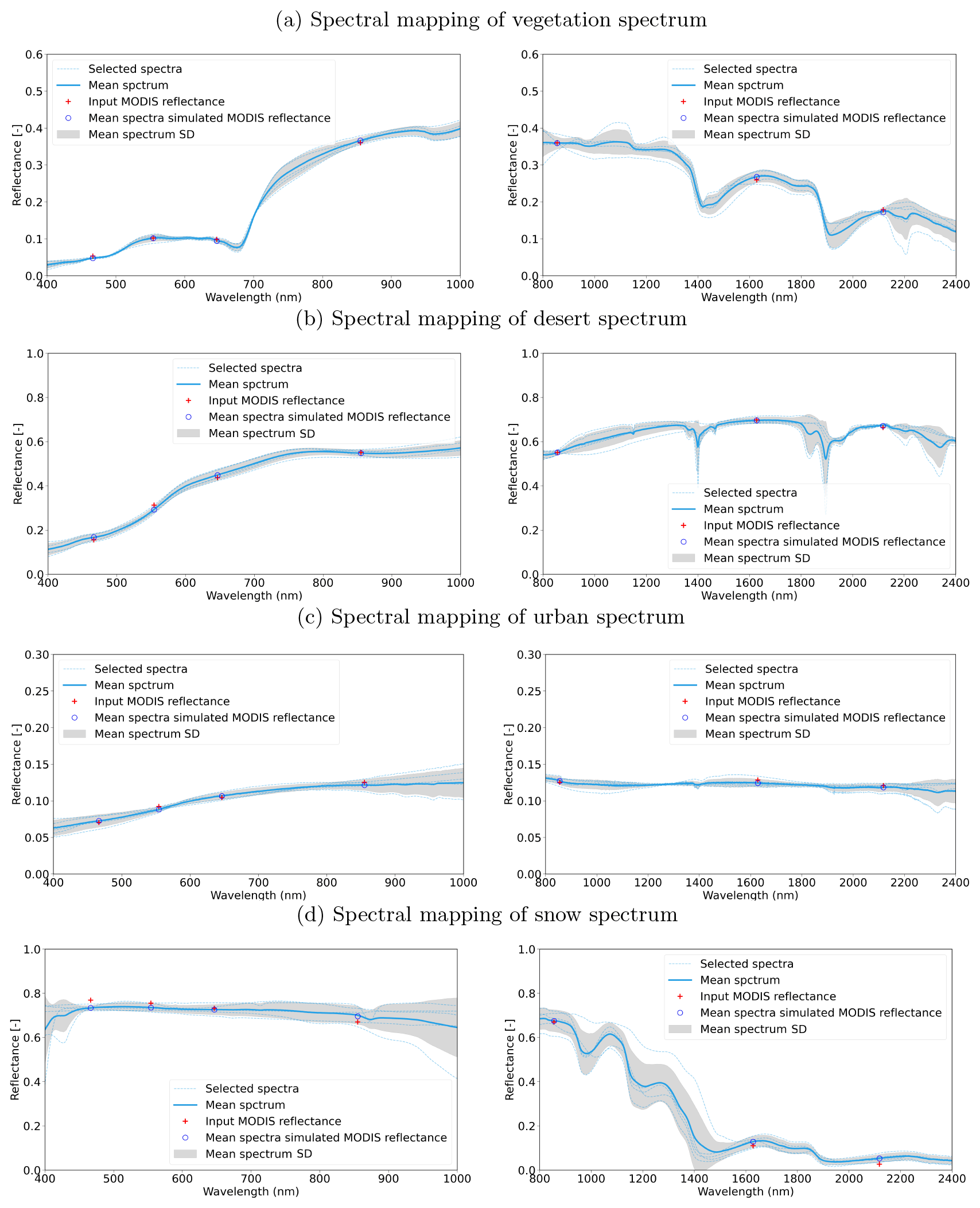
Figure D1Example of spectra selection and comparison between the MCD43-simulated reflectance and mean spectra-simulated reflectance.
The dataset used to define these transformations is derived from merging multiple spectral libraries covering the target spectral range, re-sampled to 1 nm resolution. To emphasise the importance of vegetation and soils, simulated vegetation spectra using the PROSAIL model (Jacquemoud et al., 2009) and a soil database were also used. In total, more than 6 500 spectra were used. The libraries used are shown in Table D1.
Kokaly et al. (2017)Baldridge et al. (2009)Ilehag et al. (2019)Garrity and Bindraban (2004)Table D1List of spectral libraries used to define spectral transformations.
N/A: not applicable.

Figure D2S2 (a) and L8 (b) reflectance predicted by MODIS Aqua-selected spectra from the spectral library. The uncertainty is shown with 1σ range. The original values are from the direct simulated reflectance by applying S2 and L8 RSR to the individual spectrum in the spectra library.
Given that the MODIS land bands are designed to capture most of the land surface properties, spectra selected with MODIS bands should be able to predict other optical sensors' reflectances with similar bands. Although there is a large number of spectra in the spectra library introduced in Table D1, it is still not sufficient to cover the vast variations of reflectance seen over the land surface. To deal with this limitation, the spectral searching procedure is split into two parts: visible and infrared spectral region. The spectral selection and comparison between the MODIS reflectance and mean spectra-simulated MODIS reflectance are shown in Fig. D1.
A set of five closest spectra from the spectral library are used to compute the weighted mean using an inverse distance weighting. This added number of samples introduces robustness to errors in both the MODIS surface reflectance input and the spectral library. Other numbers of selected spectra were tested, but it shows that spectra vastly different from the target spectrum are likely to be included if more than 10 spectra are used. Once the mean spectrum is calculated, it is then convolved with the target sensor-relative spectral responses (RSRs) to obtain the simulated surface reflectance at Λmap(rm). The difference between MODIS-measured reflectance and the mean predicted reflectance in the MODIS bands is used as an indicator of uncertainty.
To test the effectiveness of the proposed spectral mapping method, the MODIS, S2, and L8 reflectances are simulated with individual spectra from the spectral library. Then the MODIS-simulated reflectance is used to get K-nearest (K=6 in this case) neighbours spectra from the spectral library and to discard the spectra used for the computation of MODIS input reflectance, so the remaining spectra are independent from the input reflectance. The mean spectra are computed with weights computed from 1 divided by the standard Euclidean distance, and the mean spectra-simulated reflectance for MODIS, S2, and L8 are computed by convolving with their RSR function. The difference between mean spectra-simulated reflectance to the reflectance simulated with an individual spectrum in the spectra library for MODIS is used as a measure of standard error of the mean spectra-simulated reflectance. The result is shown in Fig. D2.
The spectral mapping results for S2 and L8 show that, over most of the cases, our spectral mapping can simulate both sensors well with high correlation (over 0.99 for all the bands), low RMSE (lower than 0.03 for all bands and 0.015 for the first 5 bands), and no bias introduced. The SWIR band around 2 200 nm shows the largest dispersion, which is attributed to the large variation in reflectance in this spectral region and the large difference in the band pass functions between MODIS and S2 and L8, as shown in Fig. 2.
The standard error estimated from MODIS reflectance provides a reasonably good estimation of the mean spectral estimated reflectance for S2 and L8, since a large discrepancy between simulations and observations implies that the input reflectance is not well represented in the spectral library.
D2 Results of spectral mapping
Results of the spectral mapping approach are shown in Fig. D2 over four representative land cover types (vegetation, desert, urban, and snow). In these plots, the input reflectance is derived from the MODIS MCD43 BRDF products using Eq. (4). The predicted reflectance is in line with the observations, with most of the observations falling within the predictive uncertainty envelope. In the DA system, poor matches to the spectral database will have large uncertainty, and those pixels will have a smaller impact on the inference.
Due to the large differences in the spatial resolution between the MODIS (500 m) and S2 and L8 (10, 20, and/or 30 m), the measured reflectance values from them cannot be directly compared. We model the MODIS data effective PSF and use this to convolve the high resolution data in order to make it comparable with the MODIS products. Ideally, the MODIS cross-track direction PSF is triangular and rectangular in along-track direction (Tan et al., 2006; Schowengerdt, 2006) as a result of optical PSFopt, detector PSFdet, image motion PSFim, and electronics PSFel:
where ∗ is a spatial convolution operator. In the MODIS MCD43 BRDF product, a number of individual observations are inverted together within a temporal window of 16 d. Each of the individual observations has a PSF described by Eq. (E1), but the combined product will have an effective PSF resulting from the combination of individual measurements with different angles and scanning geometries. In line with Kaiser and Schneider (2008), Duveiller et al. (2011), Mira et al. (2015), and Che et al. (2021), we assume that the effective or equivalent PSF (ePSF) for the combined product is given by a two-dimensional Gaussian function in along-track (x direction) and across-track (y direction) directions, as shown in Fig. E1;
where σx and σy are the standard deviation of the Gaussian function expressed over the satellite image pixels unit; Δx and Δy represent the shifts in along and cross directions. According to Duveiller et al. (2011) and Capderou (2005), there is also an angular deviation between the satellite orbit and the true north, which is given by
where θ is the angular deviation, i is the inclination angle, φ is the latitude, and κ is the daily recurrence frequency. Then, the rotation matrix (Rθ) is
We now have an expression that will permit the comparison of the high-resolution TOA reflectance with the coarse-resolution predictions of surface reflectance obtained from the MCD43 product propagated through the atmosphere. This step is fundamental in defining how the proposed method solves for atmospheric composition, and the equality requires that the high-resolution data (S2 and/or L8) are convolved with the ePSF. Given the disparity of spatial resolutions, the S2 and L8 PSF effect is averaged out during the aggregation and has been neglected in the modelling process.
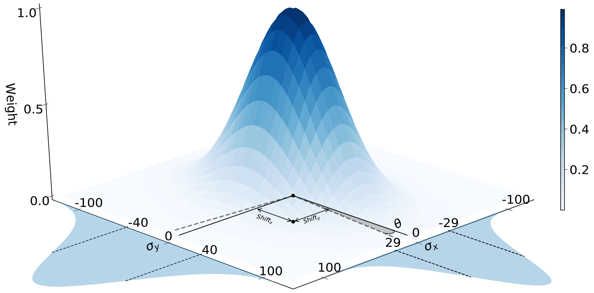
Figure E1A typical MODIS ePSF on the spatial resolution of S2, i.e. a unit of 1 represents 10 m on the X–Y plane, and it follows the same notations as in Eqs. (E2)–(E4). The shaded areas on the two sides represent the Gaussian functions used for x and y directions, with 1σ shown with vertical dashed lines.
The spatial convolution is calculated in the frequency domain for efficiency.
Results of spatial mapping (PSF)
An effective point spread function (ePSF) of the MODIS MCD43 BRDF product is simulated with a two-dimensional Gaussian function, with σx and σy controlling the widths of Gaussian in along-track and across-track directions, respectively. Shifts in those two directions are also accounted for with estimated Δx and Δy to deal with the geolocation errors in the MCD43 products. Both of the σ and Δ are in the units of pixels for the target sensor, i.e. S2 or L8.
Figure E2Comparison between MCD43-simulated surface reflectance after spectral mapping rc(Λ(m)) with S2 TOA reflectance and S2 TOA reflectance after spatial mapping on 13 April 2016 S2 50SLH tile. Top row is the rc(Λ(m)) and S2 TOA reflectance , with the scatter plot between the corresponding pixels (pixel's centre geolocation) on the right side. Bottom row is the rc(Λ(m)), with and their scatter plot.
We show an example of the PSF modelling in Fig. E2, where we compare the MCD43-predicted reflectance after spectral mapping rc(Λ(m)) with S2 TOA reflectance and after the spatial mapping at a wavelength around 2 200 nm. rc(Λ(m)) and show broadly similar coarse patterns, but higher spatial details exist . Per-pixel level comparison of them shows that rc(Λ(m)) and have a much stronger correlation, a slope very close to unity, and a bias close to 0, indicating that modelling the spatial mismatch is a required step in combining these two datasets.
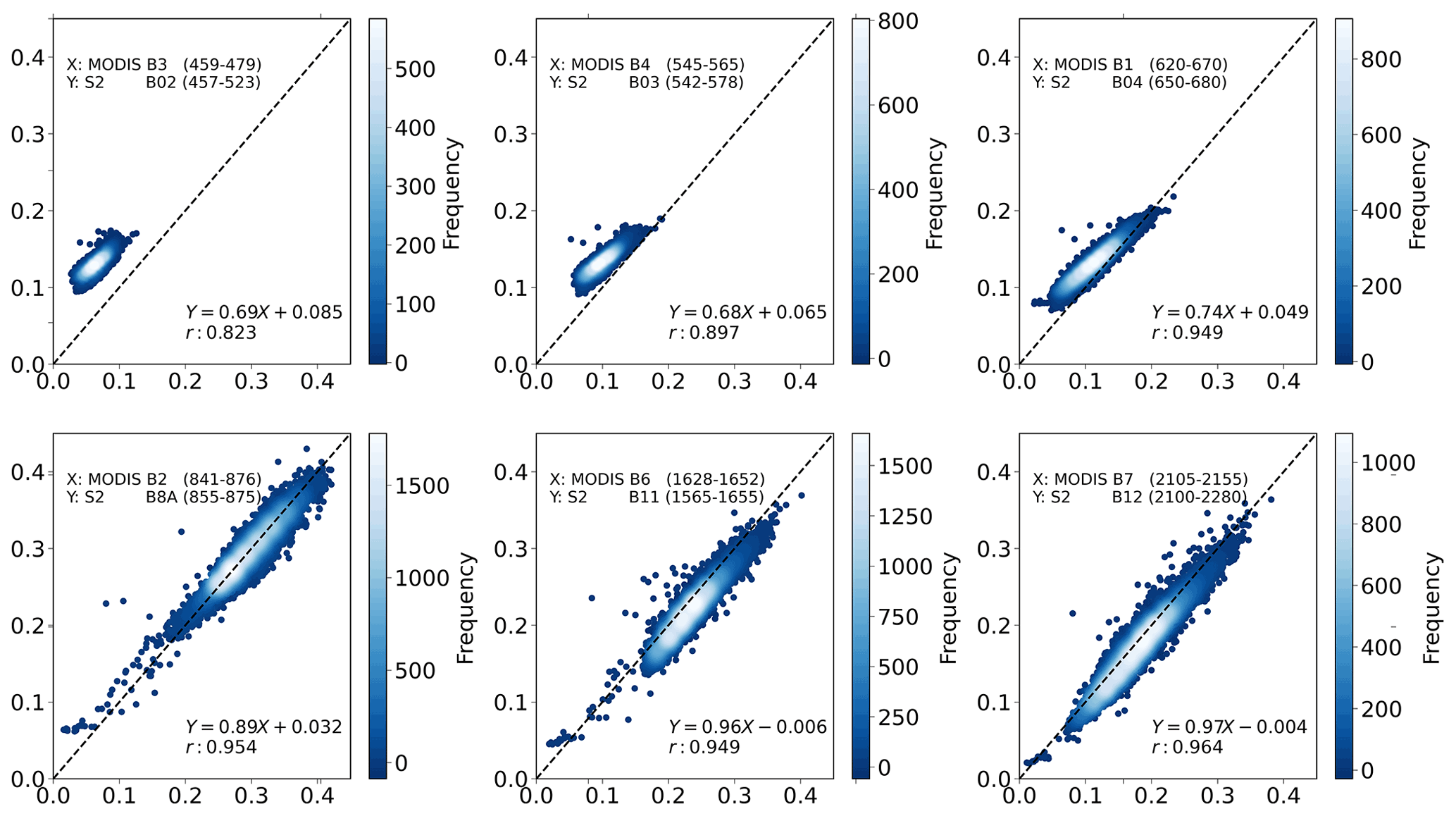
Figure E3Per-band comparison between the MCD43-simulated surface reflectancerc(Λ(m)) and at six MODIS bands.
We have assumed that, for a given scene, a single Gaussian PSF is required, in line with the findings of Mira et al. (2015), and we assume further that we can use the PSF derived for the 2 200 nm band for all other bands. At this wavelength, the atmosphere is assumed to be spatially transparent with respect to AOT, and under the spectral similarity assumption of the BRF, the results should be similar for other bands (Lyapustin et al., 2011). We illustrate the effect of atmospheric scattering by comparing the ePSF-convolved S2 TOA reflectance with the MCD43-derived BOA reflectance predictions after spectral mapping rc(Λ(m)) in Fig. E3. The pattern shows that there are consistent higher atmospheric effects for the shorter wavelengths that result in both a clear bias due to the important effect of aerosols in the intrinsic path radiance and a slope different to unity (due to the effect of aerosols on upward and downward atmospheric transmission and spherical albedo). For the longer wavelength bands after the NIR plateau, aerosol effects are less important, and the slope is close to unity and the bias close to 0, with the correlation generally being very high, and this also proves the validity of using PSF derived for the 2 200 nm band for all other bands.
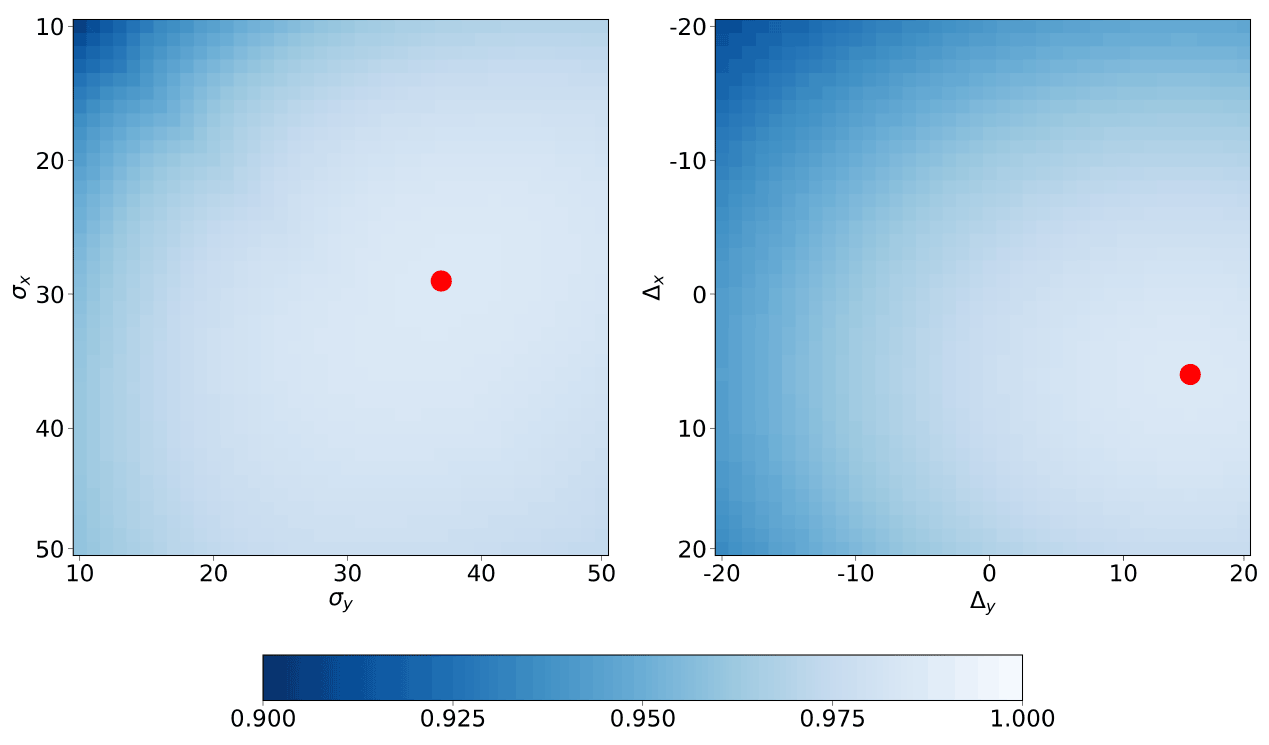
Figure E4The correlation map between rc(Λ(m)) with , with different σx, σy, Δx, and Δy values, in which the red dots represent the largest correlation values' positions.
Figure E5The density scatter plots of solved PSF parameters, σ (a, c) and Δ (b, d) in x and y direction for L8 (a, b) and S2 (c, d), where the red markers stand for the median of those parameters. The units of the x and y axis are the number of pixels.
After solving for the ePSF parameters over a large number of S2 and L8 scenes globally, we note that some simplifications in the processing are possible. First, we see that the cost function is very flat around the minimum. Figure E4 shows an example of this: for both S2 and L8, the region around the maximum correlation point has similar values (in excess of 0.98) to the maximum, suggesting that the cost function has limited sensitivities to the ePSF widths when it is close to some optimal values. A second important point is that the width of the ePSF over a large number of scenes tends to be well defined (see Fig. E5 for an example of this). For S2, the median of σx is around 26 (260 metres), and the median of σy is around 34 (340 m). For L8, these numbers are similar; only, in this case, the number of pixels is 3 times larger to account for the higher spatial resolution of S2. The shift, however, appears to be more scene dependent and also shows a larger influence on the correlation cost function.
The points made above suggest that a fixed value of 260 m for σx and 340 m for σy may be used for all images, but the effect of the pixel shift needs to be inferred on a scene-by-scene basis. We have not said much of rotation angle θ (introduced in Eq. E3). In all cases we studied, its value is small (around ±8∘), and because of the large size of the ePSF, its effect can be effectively compensated by Δx,y. It is important to note that the aim here is to provide an estimate of an effective PSF that allows a comparison between estimates of coarse-resolution surface reflectance propagated to TOA and measurements of TOA reflectance convolved with the ePSF. To further reduce the computational burden of calculating the ePSF parameters, we have taken the median of σx and σy as a reference, assumed the rotation angle of ePSF to be 0∘, and only solved for Δx,y on a scene-by-scene basis.
In this section, we illustrate cases of SIAC being used to infer atmospheric composition parameters. Due to S2 and L8 having bands outside of the strong O3 absorption region, TCO3 is taken from CAMS, and only AOT and TCWV are inferred from the data. Figure F1 shows a demonstration of the procedure. Here, an image captured over the North China Plain (tile 50SMH) by S2 on 10 February 2016 has been processed. The CAMS prior mean AOT in Fig. F1 is around 1 and is approximately constant over the scene. The TOA reflectance for band 1 of the S2 sensor (shown in log-transformed units to enhance the dynamic range) shows two clear high-aerosol stripes. The true-colour TOA image shows a very strong atmospheric effect, consistent with the expectation of high AOT. The retrieved AOT (bottom left panel in Fig. F1) shows a marked departure from the prior value. Two very high aerosol stripes are clearly resolved. The result of applying the atmospheric correction results in an important reduction of the atmospheric effects is particularly evident from the BOA true-colour composite (bottom right panel of Fig. F1).
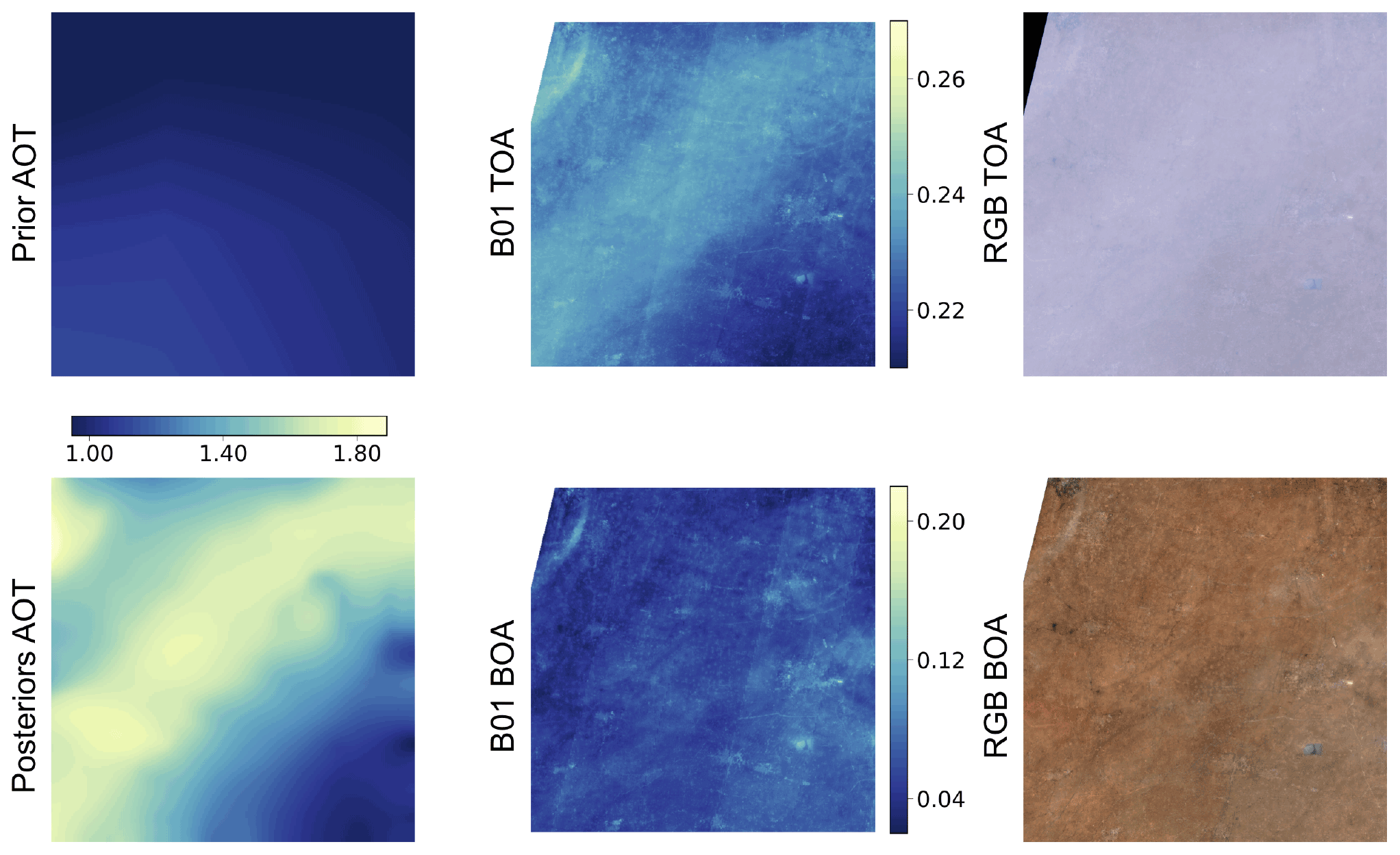
Figure F1The prior and posterior AOT over S2 50SMH on 10 February 2016 and their shared colour bar are in the first column. Figures in the second column are band 1 TOA and surface reflectance, while the TOA and BOA RGB images are shown in the third column for the same tile over the same time.
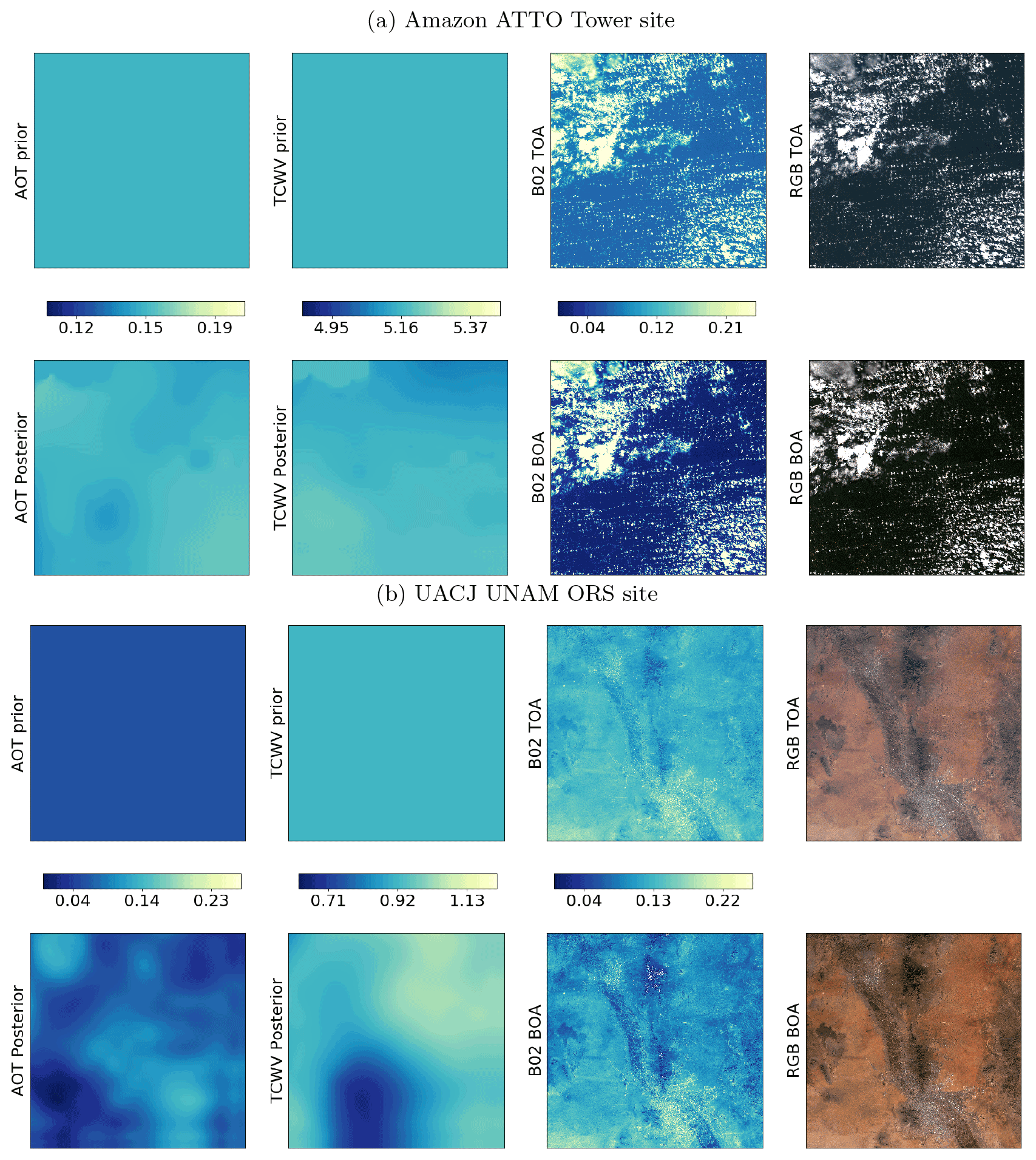
Figure F2Example of retrieval on S2 data over (a) Amazon ATTO Tower site (S2 Tile 21MTT, 27 June 2019, top row) and (b) UACJ UNAM OR site (S2 tile 13SCR, 14 January 2019, bottom row). Top row of each panel, left to right: AOT prior mean from CAMS, TCWV prior mean from CAMS, blue band TOA reflectance, TOA RGB composite. Bottom row of each panel, left to right: a posteriori AOT mean, a posteriori TCWV mean, blue band BOA reflectance, BOA RGB composite.

Figure F3Example of retrieval on S2 data over (a) XiangHe site (S2 tile 50TMK, 13 May 2019, top row) and (b) Evora site (S2 tile 29SNC, 29 July 2018). Top row of each panel, left to right: AOT prior mean from CAMS, TCWV prior mean from CAMS, blue band TOA reflectance, TOA RGB composite. Bottom row of each panel, left to right: a posteriori AOT mean, posterior TCWV mean, blue band BOA reflectance, BOA RGB composite.
Some artefacts are also apparent. In the bottom right corner of the scene, the AOT map reverts to the prior value from CAMS, which results in a poorer correction of the atmospheric effects. This is caused by lack of high quality MCD43 retrievals in this area at this time, which results in the AOT estimate being strongly driven by the prior from CAMS as well as some spatial diffusive effects from areas where the algorithm performs well. A second artefact is some visible stripes (visible in the middle top and bottom panels). These are caused by the combinations of observations from different detectors (Pahlevan et al., 2017) and have no relationship with the atmospheric correction method. It is also worth noting that, when solving for the ePSF parameters for this scene, the optimal linear correlation was only around 0.55, but clearly, the system is still able to produce reasonable results in this challenging environment.
We note that the scene shown in Fig. F1 is a challenging one: at this time of the year, most of the soil is bare, and aerosol loading is very high. Methods that rely on dark dense vegetation (DDV) exploit an empirical relationship between the reflectance around 2 200 nm and the blue and red band reflectance. If no vegetation patches are available in the scene (or if their spatial sampling is limited and aerosol spatial dynamics are high), this leads to an inability to obtain a reliable AOT estimate. The Deep Blue AOT algorithm, used in MODIS aerosol retrieval, has been developed to overcome the shortcoming of the DDV method over bright land surfaces, and the combined products deliver global coverage (Levy et al., 2013; Hsu et al., 2004, 2006). But those two methods have different assumptions and a resulting inconsistency in the merged product, especially over the transition regions which have comparatively low vegetation cover (Levy et al., 2013).
As a further illustration of the approach on Sentinel 2 data, we show similar visualisations of AOT and TCWV priors, the associated posteriors, TOA and BOA blue band reflectance, and TOA and BOA true-colour composites for a number of different sites spanning the globe in Fig. F2 (Amazon ATTO Tower and UACJ UNAM OR), Fig. F3 (XiangHe and Evora). While the effect of the atmospheric correction is evident in all these cases, it is important to note that the prior mean is significantly updated when the posterior mean of both AOT and TCWV are calculated. Spatial patterns are clearly visible in all the examples for both parameters, and in many cases, the average value from CAMS changes substantially when the proposed method is deployed. Since the retrieval are made with land pixels only, large water body pixels are filled with median aerosol values from all the land pixel retrievals, and the edge between land and water is expected.
To estimate atmospheric parameters, an estimate of surface reflectance is needed. This estimate is different from the actual surface reflectance and is likely to contain spatial artefacts, which will result in an unrealistic and noisy estimation of atmospheric parameters if an independent pixel-level retrieval strategy is used. To counter this, most practical approaches average the estimation of surface reflectance over a spatial window of fixed size. Within this window or block, atmospheric composition is assumed to be constant and inferred (Remer et al., 2009) to reduce the noise in the estimated surface reflectance. This is pragmatic in many ways and compartmentalises the processing requirements to blocks of that window size. However, the block structure imposed can introduce spurious artefacts if the spatial gradient of atmospheric parameters is large and fails to estimate atmospheric parameters when no valid targets are found within the specified box.
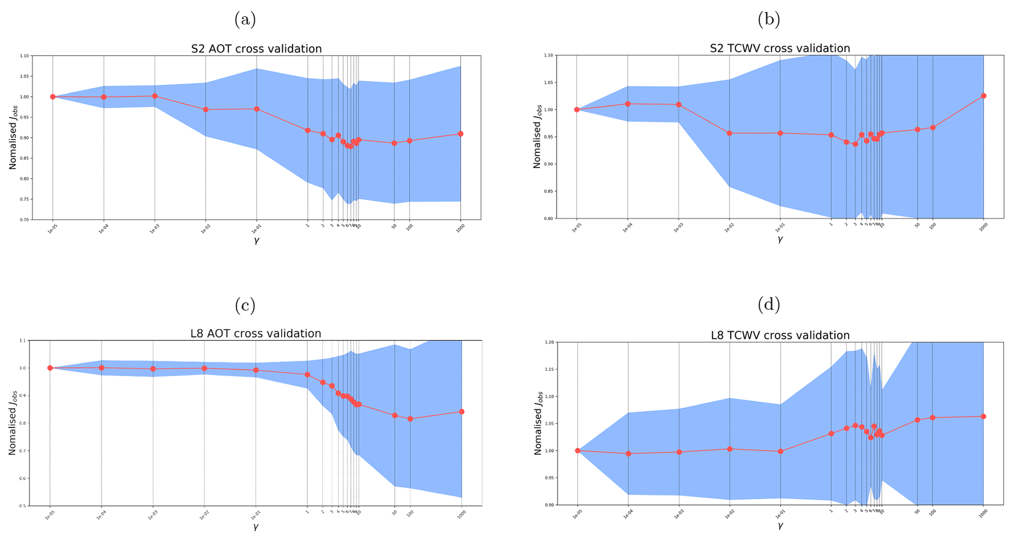
Figure G1γ cross validation for (a) S2 AOT, (b) S2 TCWV, (c) L8 AOT, and (d) L8 TCWV. The x axis in the subplots is γ values ranging from (essentially, no smoothness constraint) to 1 000 (very high smoothness). The y axis shows Jobs normalised by the Jobs with a smallest γ value of . The red dots show mean normalised Jobs over a set of 20 S2 and L8 tiles. The blue fill shows ± 1 standard deviation of normalised Jobs over the 20 samples.
Within SIAC, the broad-scale (40 km) variations of atmospheric parameters are estimated from CAMS. But there are often finer-scale features that may impact our interpretation of surface reflectance, and we wish to be able to resolve these. To this end, we assume an effective resolution of Gc (500 m) for atmospheric parameters, with the smoothness constraint expressed in Eq. (6) and controlled by γ. This spatial constraint allows for gradual changes in atmospheric parameters X at the spatial resolution of Gc over the S2 and L8 image spatial extents. The values in X that we solve for in SIAC are controlled by a weighting of the location and information content of samples in Y and the assumed uncertainty of the a priori constraint that is, in essence, blurred over Gc. The degree of smoothing imposed, and so the resultant correlation length of the derived atmospheric parameters, is mainly controlled by γ. Its squared inverse, , a measure of roughness, can also be phrased as the expectation that there is no change at a scale of 500 m (Lewis et al., 2012a). Despite this physical understanding of γ, it is not straightforward to arrive at a reasonable global estimate of this parameter. We know that too low a value means that X may become oversensitive to the sample location of the observational constraints and fail to exploit the spatial correlations we know to exist in atmospheric parameters. Too high a value will overly smooth X, and it will not be responsive to actual variations over the scene. Fortunately, we know from previous studies (e.g. Eilers, 2003; Lewis et al., 2012a; Eilers et al., 2017) that results should not be very sensitive to the precise value used and that there should be quite a wide range of tolerance. In that case, we should select the lowest tolerable value of γ. In this context, we can use a cross validation approach over a representative set of scenes to gauge a useful global value. What we would expect to assess from such an experiment is the range of tolerable γ values we might use, from which we can select the lowest tolerable value to use within SIAC. In ideal circumstances, we would see a broad but well-defined minimum in cross-validation cost. An absence of that would suggest a lack of sensitivity of the results to the selection of γ. Ideally, we would use a consistent γ value across different sensors, so that we could have the same assumed degree of smoothing.
We performed a cross validation study using 20 scenes in L8 and in S2, selected to cover a good dynamic range in AOT (0–2). We sampled over γ values from (very low) to 1 000 (very high). For each scene and for each γ value we randomly masked half of the samples in Yc, then solved for X using SIAC. With this X, we calculated the observation cost 𝒥obs according to Eq. (2) for the masked samples in Yc. This gives a measure of observation prediction error (relative to uncertainty) for samples that have atmospheric state interpolated by the correlation function for each scene for given γ. For very low γ, the influence of observational samples on the predicted atmospheric state at masked locations will be low, and at these sites, X would effectively be Xb. As γ increases, the influence of observational samples is higher, and we expect to get a better-resolved estimate of X, until a point where we are smoothing so much that we lose that resolution. In our experiments, we performed the calculation of 𝒥obs over 10 random realisations of the masking to obtain an aggregate discrepancy for each scene, normalise this measure by that of the value for the lowest γ used, then examine the mean and standard deviation of this measure of cross-validation error over the 20 scenes. The results are shown in Fig. G1.
There is mostly more variation in 𝒥obs over the scenes as γ increases, partly due to the normalisation performed, and some sampling noise in the average cost (red points and line); but, as expected, we see a broad minimum region for AOT for S2 and L8 and for TCWV for S2. For L8 TCWV, the result is more complex, and we see an increase in cross-validation error for values of γ above 0.1. This is because there is very limited sensitivity in the L8 spectral bands to TCWV. For low γ (up to 0.1 here), we are effectively seeing the cross-validation error resulting from Xb only. Beyond this point, we are over-smoothing the information in Xb, so a global γ of 0.1 for L8 TCWV is appropriate. For the other conditions, a compromise value of 5 can be considered as providing a consistent value for use over AOT for both sensors as well as S2 TCWV, although lower values of γ for S2 TCWV might also be considered from these results. In the main results section, we use other approaches to verify that these choices are appropriate using other criteria.
We show the σ of normalised error as a function of TOA reflectance uncertainty in Fig. H1. By changing the TOA reflectance uncertainty to 3 %, except for B12 (4.5 %), we can achieve the optimal uncertainty for the surface reflectance when the normalised error distributions have σ of 1. This is in line with the validation of L1C products, where the TOA reflectance can achieve 3 % (target) of uncertainty most of the time (Lamquin et al., 2018, 2019). The result for L8 is similar to S2, but it is worth mentioning that the optimal uncertainties for L8 TOA are less than 3 % for all the bands, with the max being around 2.5 %. This could be attributed to the fact that fewer co-incident L8 and RadCalNet measurement samples are available due to its longer global revisit time.
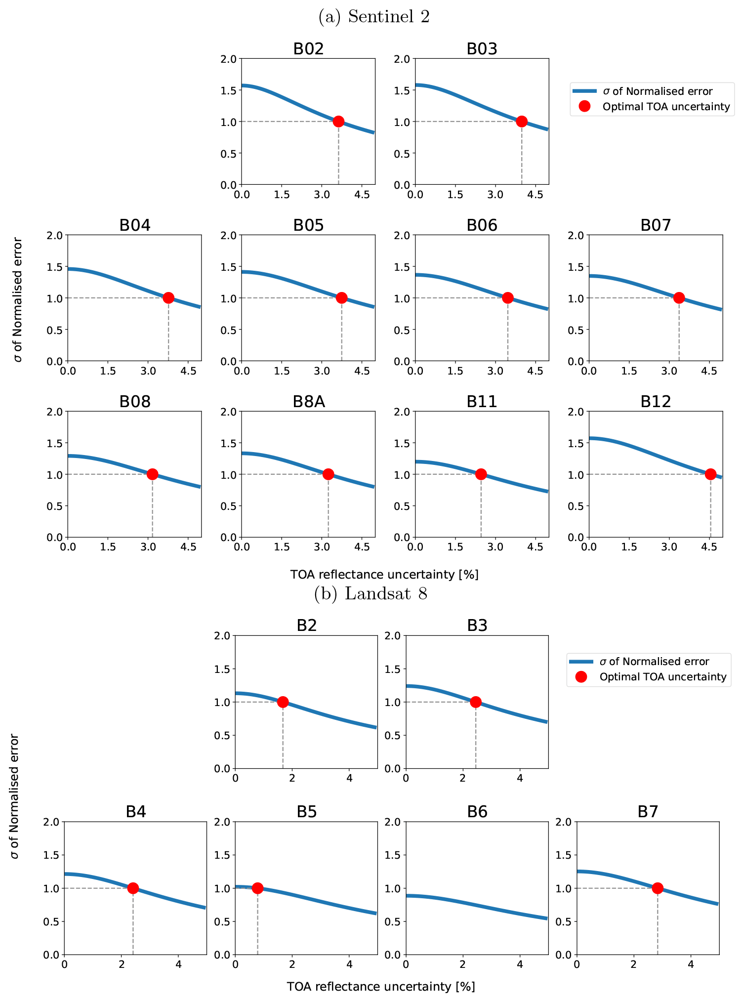
Figure H1Surface reflectance normalised error distribution as a function of TOA reflectance uncertainty. The red dot indicates the point by changing the TOA uncertainty to reach the optimal uncertainty (σ of 1 for the normalised error distribution). B6 for L8 in (b) has σ smaller than 1 for all the time and so cannot determine the optimal σ.
We show the correction done by only using the prior values from CAMS predictions in Figs. I1, I2, and I3. For most of the time, the CAMS prior-corrected reflectances match the RadCalNet measurements well, but they are worse than the corrections done with SIAC, shown in Figs. 11, 12 and 13, though the differences are small. This is because those RadCalNet sites are located in places with homogeneous landscapes and mostly low aerosol loading (RadCalNet, 2018a). Considering the low sensitivity of surface reflectance to low aerosol loading atmosphere condition, the improvement made on AOT estimation will not improve much on the mean of the estimated surface reflectance. This suggests that the current RadCalNet sites can only be used as a minimum quality check of atmospheric correction or land surface reflectance. More challenging and heterogeneous surface conditions are required for the evaluation of surface reflectance quality. The uncertainty comparison between the prior (CAMS) and posterior (SIAC) corrected surface reflectance in Fig. I4 shows that the improvements on the uncertainty budget are around 10 % for visible to near-infrared bands and 5 % for SWIR bands for TOA uncertainty of 5 % to 2.5 %. The uncertainty improvement result for L8 is much more subtle; this could be attributed to the small sample size. It is also interesting to note that the surface reflectance uncertainty is a function of TOA uncertainty, and the proportion of improvements depends on the relative weight between the atmospheric parameters' uncertainty and the TOA uncertainty.
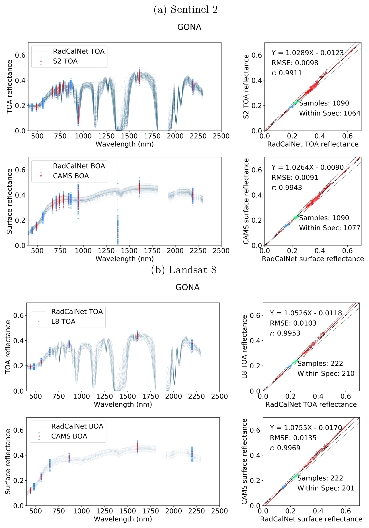
Figure I1Comparison between the S2 (a) and L8 (b) TOA reflectance and RadCalNet simulated nadir-view TOA reflectance (top row), and the surface reflectance after correction with CAMS prior against RadCalNet nadir-view surface reflectance (bottom row) at Gobabeb. The blue lines on the left are different spectra measurements from RadCalNet, and the red dots with blue error bars (1 standard deviation) are the TOA or surface and TOA reflectance with uncertainty. The threshold uncertainty is given as black dashed lines in the scatter plots. The regression line is drawn as a red line, and the 1-to-1 reference line is drawn as a thick black dashed line in the middle.


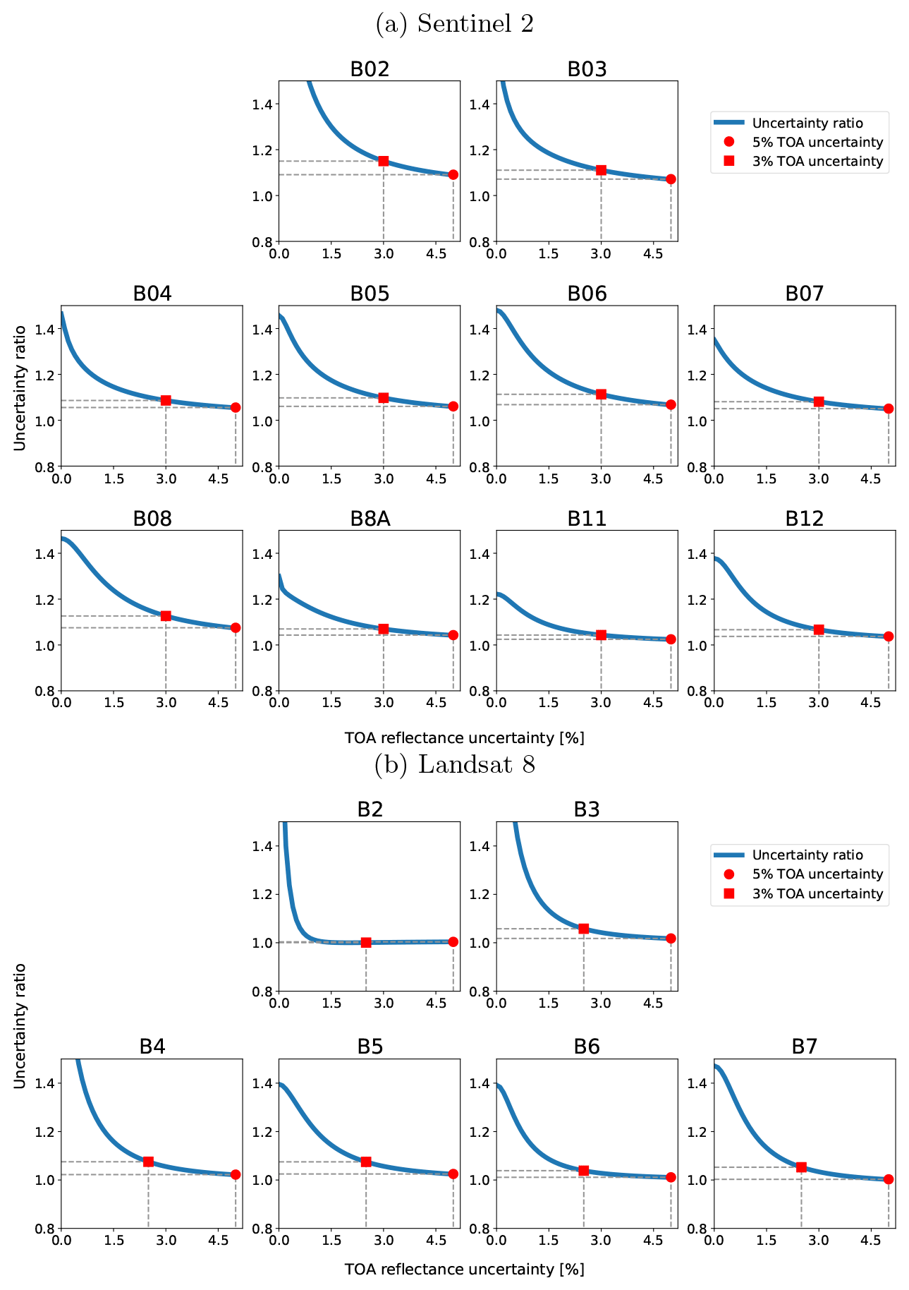
Figure I4Surface reflectance uncertainty comparison between CAMS prior corrections and SIAC corrections. The ratio is calculated as CAMS prior-corrected surface reflectance uncertainty divided by SIAC surface reflectance uncertainty for different values of TOA uncertainty. The red dot indicates the uncertainty ratio when 5 % of the TOA reflectance uncertainty is used, while the red square indicates the uncertainty ratio when 3 % of the TOA reflectance is uncertainty used.
The code for SIAC is written in Python and is released under the GPLv3 open source licence. The code is available through the Zenodo from https://doi.org/10.5281/zenodo.6651964 (Yin, 2022a).
The input data are publicly available through references listed in Table 4, and the validations results over AERONET and RadCalNet sites are uploaded to Zenodo: https://doi.org/10.5281/zenodo.6652892 (Yin, 2022b).
FY and PEL conceptualised the study. FY developed the code, prepared the datasets, and analysed the results. FY and PEL wrote the manuscript. JLGD suggested experiments and contributed to the drafting of the manuscript. All authors contributed to editing the paper.
The contact author has declared that none of the authors has any competing interests.
Publisher's note: Copernicus Publications remains neutral with regard to jurisdictional claims in published maps and institutional affiliations.
The authors would like to acknowledge financial support from the European Union Horizon 2020 research and innovation programme under grant agreement no. 687320 MULTIPLY (MULTIscale SENTINEL land surface information retrieval Platform) and from the European Space Agency (ESA) under contract no. 4000112388/14/I-NB SEOM SY-4Sci Synergy. Feng Yin, Philip E. Lewis, and Jose L. Gómez-Dans were supported by the Natural Environment Research Council's (NERC) National Centre for Earth Observation (NCEO) (project no. 525861). Feng Yin and Philip E. Lewis were supported by Science and Technology Facilities Council (STFC) of UK-Newton Agritech Programme (project no. 533651).
This research has been supported by the European Commission, Horizon 2020 (MULTIPLY (grant no. 687320)), the European Space Agency (grant no. 4000112388/14/I-NB SEOM SY-4Sci Synergy), the National Centre for Earth Observation (grant no. 525861), and the Science and Technology Facilities Council (STFC) of UK-Newton Agritech Programme (project no. 533651).
This paper was edited by Le Yu and reviewed by three anonymous referees.
AERONET: Aerosol Robotic Network (AERONET) Homepage, https://aeronet.gsfc.nasa.gov/ (last access: 21 October 2022), 2021. a, b
Anderson, T. L., Charlson, R. J., Winker, D. M., Ogren, J. A., and Holmén, K.: Mesoscale variations of tropospheric aerosols, J. Atmos. Sci., 60, 119–136, 2003. a, b
Baetens, L. and Hagolle, O.: Sentinel-2 reference cloud masks generated by an active learning method, Zenodo [data set], https://doi.org/10.5281/ZENODO.1460961, 2018. a
Baldridge, A., Hook, S., Grove, C., and Rivera, G.: The ASTER spectral library version 2.0, Remote Sens. Environ., 113, 711–715, https://doi.org/10.1016/j.rse.2008.11.007, 2009. a, b
Barsi, J. A., Alhammoud, B., Czapla-Myers, J., Gascon, F., Haque, M. O., Kaewmanee, M., Leigh, L., and Markham, B. L.: Sentinel-2A MSI and Landsat-8 OLI radiometric cross comparison over desert sites, Eur. J. Remote Sens., 51, 822–837, https://doi.org/10.1080/22797254.2018.1507613, 2018a. a
Barsi, J. A., Alhammoud, B., Czapla-Myers, J., Gascon, F., Haque, M. O., Kaewmanee, M., Leigh, L., and Markham, B. L.: Sentinel-2A MSI and Landsat-8 OLI radiometric cross comparison over desert sites, Eur. J. Remote Sens., 51, 822–837, 2018b. a
Benedetti, A., Morcrette, J.-J., Boucher, O., Dethof, A., Engelen, R. J., Fisher, M., Flentje, H., Huneeus, N., Jones, L., Kaiser, J. W, and Kinne, S.: Aerosol analysis and forecast in the European centre for medium-range weather forecasts integrated forecast system: 2. Data assimilation, J. Geophys. Res.-Atmos., 114, D13205, https://doi.org/10.1029/2008jd011115, 2009. a, b, c
Bouvet, M., Thome, K., Berthelot, B., Bialek, A., Czapla-Myers, J., Fox, N. P., Goryl, P., Henry, P., Ma, L., Marcq, S., and Meygret, A.: RadCalNet: A radiometric calibration network for earth observing imagers operating in the visible to shortwave infrared spectral range, Remote Sens., 11, 2401, https://doi.org/10.3390/rs11202401, 2019. a, b
Briggs, W. L., Henson, V. E., and McCormick, S. F.: A Multigrid Tutorial, Second Edition, Society for Industrial and Applied Mathematics, https://doi.org/10.1137/1.9780898719505, 2000. a
Byrd, R. H., Lu, P., Nocedal, J., and Zhu, C.: A Limited Memory Algorithm for Bound Constrained Optimization, SIAM J. Sci. Comput., 16, 1190–1208, https://doi.org/10.1137/0916069, 1995. a
Capderou, M.: Satellites: Orbits and Missions, Springer, https://doi.org/10.1007/b139118, 2005. a
CEOS: CEOS Analysis Ready Data Strategy, http://ceos.org/ard/files/CEOS_ARD_Strategy_v1.0_1-Oct-2019.pdf (last access: 3 March 2020), 2019. a
CEOS: CEOS Analysis Ready Data Surface Reflectance Specification, https://ceos.org/ard/files/PFS/SR/v5.0/CARD4L_Product_Family_Specification_Surface_Reflectance-v5.0.pdf, last access: 25 January 2020. a
CEOS: WGCV CARD4L Review Panel evaluation (SR PFS v5), CEOS, https://ceos.org/ard/files/Self%20Assessments/SR/v5.0/WGCV_CARD4L_Review_Panel_Assessment_USGS_SR_PFS_v5.pdf (last access: 21 October 2022), 2021a. a
CEOS: CEOS Analysis Ready Data, https://ceos.org/ard, last access: 21 September 2021b. a
CEOS: Analysis Ready Data For Land, https://ceos.org/ard/files/PFS/SR/v5.0/CARD4L_Product_Family_Specification_Surface_Reflectance-v5.0.pdf (last access: 21 October 2022), 2021c. a
Chatterjee, A., Michalak, A. M., Kahn, R. A., Paradise, S. R., Braverman, A. J., and Miller, C. E.: A geostatistical data fusion technique for merging remote sensing and ground-based observations of aerosol optical thickness, J. Geophys. Res.-Atmos., 115, D20207, https://doi.org/10.1029/2009JD013765, 2010. a
Che, X., Zhang, H. K., and Liu, J.: Making Landsat 5, 7 and 8 reflectance consistent using MODIS nadir-BRDF adjusted reflectance as reference, Remote Sens. Environ., 262, 112517, https://doi.org/10.1016/j.rse.2021.112517, 2021. a
Chen, J. and Zhu, W.: Comparing Landsat-8 and Sentinel-2 top of atmosphere and surface reflectance in high latitude regions: case study in Alaska, Geocarto International, 37, 6052–6071, https://doi.org/10.1080/10106049.2021.1924295, 2021. a
Clerc, S. and MPC Team: Sentinel-2 L1C data quality report, ESA, Tech. Rep, 59, 2021. a
Doxani, G., Vermote, E., Roger, J.-C., Gascon, F., Adriaensen, S., Frantz, D., Hagolle, O., Hollstein, A., Kirches, G., Li, F., Louis, J., Mangin, A., Pahlevan, N., Pflug, B., and Vanhellemont, Q.: Atmospheric Correction Inter-Comparison Exercise, Remote Sens., 10, 352, https://doi.org/10.3390/rs10020352, 2018. a, b, c
Doxani, G., Vermote, E., Roger, J.-C., Skakun, S., Gascon, F., Collison, A., Keukelaere, L. D., Desjardins, C., Frantz, D., Hagolle, O., Kim, M., , Louis, J., Pacifici, F., Pflug, B., Poilvé, H., Ramon, D., Richter, R., and Yin, F.: Atmospheric Correction Inter-Comparison eXercise (ACIX II Land): an atmospheric correction processors assessment for Landsat 8 and Sentinel-2 over land, Remote Sens. Environ., in review, 2022. a, b, c, d
Dubovik, O., Herman, M., Holdak, A., Lapyonok, T., Tanré, D., Deuzé, J. L., Ducos, F., Sinyuk, A., and Lopatin, A.: Statistically optimized inversion algorithm for enhanced retrieval of aerosol properties from spectral multi-angle polarimetric satellite observations, Atmos. Meas. Tech., 4, 975–1018, https://doi.org/10.5194/amt-4-975-2011, 2011. a, b, c
Dubovik, O., Lapyonok, T., Litvinov, P., Herman, M., Fuertes, D., Ducos, F., Lopatin, A., Chaikovsky, A., Torres, B., Derimian, Y., Huang, X., Aspetsberger, M., and Federspie, C.: GRASP: a versatile algorithm for characterizing the atmosphere, sPIE: Newsroom, https://doi.org/10.1117/2.1201408.005558, 2014. a
Duveiller, G., Baret, F., and Defourny, P.: Crop specific green area index retrieval from MODIS data at regional scale by controlling pixel-target adequacy, Remote Sens. Environ., 115, 2686–2701, https://doi.org/10.1016/j.rse.2011.05.026, 2011. a, b
Eck, T. F., Holben, B., Reid, J., Dubovik, O., Smirnov, A., O'neill, N., Slutsker, I., and Kinne, S.: Wavelength dependence of the optical depth of biomass burning, urban, and desert dust aerosols, J. Geophys. Res.-Atmos., 104, 31333–31349, 1999. a
Eilers, P. H.: A perfect smoother, Anal. Chem., 75, 3631–3636, 2003. a
Eilers, P. H., Pesendorfer, V., and Bonifacio, R.: Automatic smoothing of remote sensing data, in: 2017 9th International Workshop on the Analysis of Multitemporal Remote Sensing Images (MultiTemp), IEEE, 1–3, 2017. a
ESA: Sentinel-2, https://sentinel.esa.int/web/sentinel/missions/sentinel-2 (last access: 21 October 2022), 2015. a
ESA: Land Cover CCI Product User Guide Version 2 Tech. Rep., http://maps.elie.ucl.ac.be/CCI/viewer/download/ESACCI-LC-Ph2-PUGv2_2.0.pdf, (last access: 22 September 2021), 2017. a, b
ESA: Gearing up for third Sentinel-2 satellite, ESA, https://www.esa.int/Applications/Observing_the_Earth/Copernicus/Sentinel-2/Gearing_up_for_third_Sentinel-2_satellite (last access: 21 October 2022), 2021a. a
ESA: S2 MPC Level-2A Algorithm Theoretical Basis Document, https://sentinel.esa.int/documents/247904/4363007/Sentinel-2-Level-2A-Algorithm-Theoretical-Basis-Document-ATBD.pdf/fe5bacb4-7d4c-9212-8606-6591384390c3 (last access: 21 October 2022), 2021b. a
ESA: S2 MPC Level-2A Algorithm Theoretical Basis Document, https://step.esa.int/thirdparties/sen2cor/2.10.0/docs/S2-PDGS-MPC-L2A-ATBD-V2.10.0.pdf (last access: 21 October 2022), 2021c. a
Feng, M., Sexton, J. O., Huang, C., Masek, J. G., Vermote, E. F., Gao, F., Narasimhan, R., Channan, S., Wolfe, R. E., and Townshend, J. R.: Global surface reflectance products from Landsat: Assessment using coincident MODIS observations, Remote Sens. Environ., 134, 276–293, https://doi.org/10.1016/j.rse.2013.02.031, 2013. a
Flood, N.: Comparing Sentinel-2A and Landsat 7 and 8 using surface reflectance over Australia, Remote Sens., 9, 659, https://doi.org/10.3390/rs9070659, 2017. a
Foga, S., Scaramuzza, P. L., Guo, S., Zhu, Z., Dilley Jr., R. D., Beckmann, T., Schmidt, G. L., Dwyer, J. L., Hughes, M. J., and Laue, B.: Cloud detection algorithm comparison and validation for operational Landsat data products, Remote Sens. Environ., 194, 379–390, 2017. a
Franch, B., Vermote, E., Sobrino, J., and Fédèle, E.: Analysis of directional effects on atmospheric correction, Remote Sens. Environ., 128, 276–288, https://doi.org/10.1016/j.rse.2012.10.018, 2013. a, b
Francis, A., Mrziglod, J., Sidiropoulos, P., and Muller, J.-P.: Sentinel-2 Cloud Mask Catalogue, Zenodo [data set], https://doi.org/10.5281/ZENODO.4172871, 2020. a
Garcia, D.: Robust smoothing of gridded data in one and higher dimensions with missing values, Comput. Stat. Data Anal., 54, 1167–1178, 2010. a, b, c, d
Garrity, D. and Bindraban, P.: A globally distributed soil spectral library visible near infrared diffuse reflectance spectra, ICRAF (World Agroforestry Centre)/ISRIC (World Soil Information) Spectral Library: Nairobi, Kenya, 2004. a, b
Gascon, F., Bouzinac, C., Thépaut, O., Jung, M., Francesconi, B., Louis, J., Lonjou, V., Lafrance, B., Massera, S., Gaudel-Vacaresse, A., and Languille, F.: Copernicus Sentinel-2A calibration and products validation status, Remote Sens., 9, 584, https://doi.org/10.3390/rs9060584, 2017. a
GCOS: Albedo ESSENTIAL CLIMATE VARIABLE (ECV) FACTSHEET, https://gcos.wmo.int/en/essential-climate-variables/albedo (last access: 12 September 2022), 2019. a
Giles, D. M., Sinyuk, A., Sorokin, M. G., Schafer, J. S., Smirnov, A., Slutsker, I., Eck, T. F., Holben, B. N., Lewis, J. R., Campbell, J. R., Welton, E. J., Korkin, S. V., and Lyapustin, A. I.: Advancements in the Aerosol Robotic Network (AERONET) Version 3 database – automated near-real-time quality control algorithm with improved cloud screening for Sun photometer aerosol optical depth (AOD) measurements, Atmos. Meas. Tech., 12, 169–209, https://doi.org/10.5194/amt-12-169-2019, 2019. a, b
Gómez-Dans, J. L., Lewis, P. E., and Disney, M.: Efficient Emulation of Radiative Transfer Codes Using Gaussian Processes and Application to Land Surface Parameter Inferences, Remote Sens., 8, 119, https://doi.org/10.3390/rs8020119, 2016. a, b
Govaerts, Y. and Luffarelli, M.: Joint retrieval of surface reflectance and aerosol properties with continuous variation of the state variables in the solution space – Part 1: theoretical concept, Atmos. Meas. Tech., 11, 6589–6603, https://doi.org/10.5194/amt-11-6589-2018, 2018. a, b, c
Guanter, L., Del Carmen González-Sanpedro, M., and Moreno, J.: A method for the atmospheric correction of ENVISAT/MERIS data over land targets, Int. J. Remote Sens., 28, 709–728, https://doi.org/10.1080/01431160600815525, 2007. a, b, c
Hagolle, O., Huc, M., Pascual, D., and Dedieu, G.: A Multi-Temporal and Multi-Spectral Method to Estimate Aerosol Optical Thickness over Land, for the Atmospheric Correction of FormoSat-2, LandSat, VENS and Sentinel-2 Images, Remote Sens., 7, 2668–2691, https://doi.org/10.3390/rs70302668, 2015a. a
Hagolle, O., Huc, M., Villa Pascual, D., and Dedieu, G.: A multi-temporal and multi-spectral method to estimate aerosol optical thickness over land, for the atmospheric correction of FormoSat-2, LandSat, VENμS and Sentinel-2 images, Remote Sens., 7, 2668–2691, 2015b. a, b, c
Hall, D. K. and Riggs, G. A.: Normalized-Difference Snow Index (NDSI), in: Encyclopedia of Earth Sciences Series, Springer Netherlands, 779–780, https://doi.org/10.1007/978-90-481-2642-2_376, 2011. a
Hecht-Nielsen, R.: Theory of the backpropagation neural network, in: Neural networks for perception, Academic Press, 65–93, https://doi.org/10.1109/IJCNN.1989.118638, 1992. a
Helder, D., Markham, B., Morfitt, R., Storey, J., Barsi, J., Gascon, F., Clerc, S., LaFrance, B., Masek, J., Roy, D., Lewis, A., and Pahlevan, N.: Observations and Recommendations for the Calibration of Landsat 8 OLI and Sentinel 2 MSI for Improved Data Interoperability, Remote Sens., 10, 1340, https://doi.org/10.3390/rs10091340, 2018. a
Hilker, T.: Chapter 3.02 – Surface Reflectance/Bidirectional Reflectance Distribution Function, in: Comprehensive Remote Sensing, edited by: Liang, S., Elsevier, Oxford, 2–8, https://doi.org/10.1016/B978-0-12-409548-9.10347-1, 2018. a
Hou, W., Wang, J., Xu, X., Reid, J. S., Janz, S. J., and Leitch, J. W.: An algorithm for hyperspectral remote sensing of aerosols: 3. Application to the GEO-TASO data in KORUS-AQ field campaign, J. Quant. Spectrosc. Ra., 253, 107161, https://doi.org/10.1016/j.jqsrt.2020.107161, 2020. a, b
Hsu, N., Tsay, S.-C., King, M., and Herman, J.: Aerosol Properties Over Bright-Reflecting Source Regions, IEEE T. Geosci. Remote, 42, 557–569, https://doi.org/10.1109/tgrs.2004.824067, 2004. a
Hsu, N., Tsay, S.-C., King, M., and Herman, J.: Deep Blue Retrievals of Asian Aerosol Properties During ACE-Asia, IEEE T. Geosci. Remote, 44, 3180–3195, https://doi.org/10.1109/tgrs.2006.879540, 2006. a
Hsu, N. C., Jeong, M.-J., Bettenhausen, C., Sayer, A. M., Hansell, R., Seftor, C. S., Huang, J., and Tsay, S.-C.: Enhanced Deep Blue aerosol retrieval algorithm: The second generation, J. Geophys. Res.-Atmos., 118, 9296–9315, https://doi.org/10.1002/jgrd.50712, 2013. a, b
Hughes, M. J. and Hayes, D. J.: Automated detection of cloud and cloud shadow in single-date Landsat imagery using neural networks and spatial post-processing, Remote Sens., 6, 4907–4926, 2014. a
Ilehag, R., Schenk, A., Huang, Y., and Hinz, S.: KLUM: An Urban VNIR and SWIR Spectral Library Consisting of Building Materials, Remote Sens., 11, 2149, https://doi.org/10.3390/rs11182149, 2019. a, b
Jacquemoud, S., Verhoef, W., Baret, F., Bacour, C., Zarco-Tejada, P. J., Asner, G. P., François, C., and Ustin, S. L.: PROSPECT + SAIL models: A review of use for vegetation characterization, Remote Sens. Environ., 113, S56–S66, https://doi.org/10.1016/j.rse.2008.01.026, 2009. a
Justice, C. O., Román, M. O., Csiszar, I., Vermote, E. F., Wolfe, R. E., Hook, S. J., Friedl, M., Wang, Z., Schaaf, C. B., Miura, T., and Tschudi, M.: Land and cryosphere products from Suomi NPP VIIRS: Overview and status, J. Geophys. Res.-Atmos., 118, 9753–9765, 2013. a
Kaiser, G. and Schneider, W.: Estimation of sensor point spread function by spatial subpixel analysis, Int. J. Remote Sens., 29, 2137–2155, https://doi.org/10.1080/01431160701395310, 2008. a
Kaminski, T., Pinty, B., Voßbeck, M., Lopatka, M., Gobron, N., and Robustelli, M.: Consistent retrieval of land surface radiation products from EO, including traceable uncertainty estimates, Biogeosciences, 14, 2527–2541, https://doi.org/10.5194/bg-14-2527-2017, 2017. a
Kaufman, Y. J.: Aerosol optical thickness and atmospheric path radiance, J. Geophys. Res.-Atmos., 98, 2677–2692, 1993. a
Kaufman, Y. J., Tanré, D., Remer, L. A., Vermote, E. F., Chu, A., and Holben, B. N.: Operational remote sensing of tropospheric aerosol over land from EOS moderate resolution imaging spectroradiometer, J. Geophys. Res.-Atmos., 102, 17051–17067, https://doi.org/10.1029/96jd03988, 1997. a
Kokaly, R. F., Clark, R. N., Swayze, G. A., Livo, K. E., Hoefen, T. M., Pearson, N. C., Wise, R. A., Benzel, W. M., Lowers, H. A., Driscoll, R. L., and Klein, A. J.: USGS Spectral Library Version 7 Data: U.S. Geological Survey data release [data set], https://doi.org/10.5066/F7RR1WDJ, 2017. a, b
Ku, H.: Notes on the use of propagation of error formulas, J. Res. Nat. Bur. Stand., 70C, 263, https://doi.org/10.6028/jres.070c.025, 1966. a
Lamquin, N., Bruniquel, V., and Gascon, F.: Sentinel-2 L1C radiometric validation using deep convective clouds observations, Eur. J. Remote Sens., 51, 11–27, 2018. a, b
Lamquin, N., Woolliams, E., Bruniquel, V., Gascon, F., Gorroño, J., Govaerts, Y., Leroy, V., Lonjou, V., Alhammoud, B., Barsi, J. A., and Czapla-Myers, J. S.: An inter-comparison exercise of Sentinel-2 radiometric validations assessed by independent expert groups, Remote Sens. Environ., 233, 111369, 2019. a, b, c, d
Levy, R. C., Remer, L. A., and Dubovik, O.: Global aerosol optical properties and application to Moderate Resolution Imaging Spectroradiometer aerosol retrieval over land, J. Geophys. Res.-Atmos., 112, D13210, https://doi.org/10.1029/2006jd007815, 2007a. a
Levy, R. C., Remer, L. A., Mattoo, S., Vermote, E. F., and Kaufman, Y. J.: Second-generation operational algorithm: Retrieval of aerosol properties over land from inversion of Moderate Resolution Imaging Spectroradiometer spectral reflectance, J. Geophys. Res.-Atmos., 112, D13211, https://doi.org/10.1029/2006jd007811, 2007b. a
Levy, R. C., Mattoo, S., Munchak, L. A., Remer, L. A., Sayer, A. M., Patadia, F., and Hsu, N. C.: The Collection 6 MODIS aerosol products over land and ocean, Atmos. Meas. Tech., 6, 2989–3034, https://doi.org/10.5194/amt-6-2989-2013, 2013. a, b
Lewis, P., Gómez-Dans, J., Kaminski, T., Settle, J., Quaife, T., Gobron, N., Styles, J., and Berger, M.: An Earth Observation Land Data Assimilation System (EO-LDAS), Remote Sens. Environ., 120, 219–235, https://doi.org/10.1016/j.rse.2011.12.027, 2012a. a, b, c, d, e, f
Lewis, P., Guanter, L., Saldaña, G. L., Muller, J., Shane, N., Fisher, J., North, P., Heckel, A., Danne, O., and Brockmann, C.: GlobAlbedo Algorithm Theoretical Basis Document V3.1, http://www.globalbedo.org/docs/GlobAlbedo_Albedo_ATBD_V4.12.pdf (last access: 3 March 2020), 2012b. a, b
Li, Q., Li, C., and Mao, J.: Evaluation of atmospheric aerosol optical depth products at ultraviolet bands derived from MODIS products, Aerosol Sci. Technol., 46, 1025–1034, 2012. a
Li, Y., Chen, J., Ma, Q., Zhang, H. K., and Liu, J.: Evaluation of Sentinel-2A Surface Reflectance Derived Using Sen2Cor in North America, IEEE J. Sel. Top. Appl., 11, 1997–2021, https://doi.org/10.1109/jstars.2018.2835823, 2018. a
Liang, S.: Narrowband to broadband conversions of land surface albedo I: Algorithms, Remote Sens. Environ., 76, 213–238, https://doi.org/10.1016/S0034-4257(00)00205-4, 2001. a
Lipponen, A., Mielonen, T., Pitkänen, M. R. A., Levy, R. C., Sawyer, V. R., Romakkaniemi, S., Kolehmainen, V., and Arola, A.: Bayesian aerosol retrieval algorithm for MODIS AOD retrieval over land, Atmos. Meas. Tech., 11, 1529–1547, https://doi.org/10.5194/amt-11-1529-2018, 2018. a
Louis, J., Debaecker, V., Pflug, B., Main-Knorn, M., Bieniarz, J., Mueller-Wilm, U., Cadau, E., and Gascon, F.: Sentinel-2 Sen2Cor: L2A processor for users, in: Proceedings Living Planet Symposium 2016, Spacebooks Online, 1–8, https://elib.dlr.de/107381/ (last access: 22 October 2022), 2016. a
Lyapustin, A., Martonchik, J., Wang, Y., Laszlo, I., and Korkin, S.: Multiangle implementation of atmospheric correction (MAIAC): 1. Radiative transfer basis and look-up tables, J. Geophys. Res.-Atmos., 116, D03211, https://doi.org/10.1029/2010JD014986, 2011. a
Lyapustin, A., Wang, Y., Korkin, S., and Huang, D.: MODIS Collection 6 MAIAC algorithm, Atmos. Meas. Tech., 11, 5741–5765, https://doi.org/10.5194/amt-11-5741-2018, 2018. a
Masek, J., Vermote, E., Saleous, N., Wolfe, R., Hall, F., Huemmrich, F., Gao, F., Kutler, J., and Lim, T.: LEDAPS Landsat Calibration, Reflectance, Atmospheric Correction Preprocessing Code, ORNL DAAC [code], https://doi.org/10.3334/ornldaac/1080, 2012. a
Masek, J. G., Wulder, M. A., Markham, B., McCorkel, J., Crawford, C. J., Storey, J., and Jenstrom, D. T.: Landsat 9: Empowering open science and applications through continuity, Remote Sens. Environ., 248, 111968, https://doi.org/10.1016/j.rse.2020.111968, 2020. a
McGill, R., Tukey, J. W., and Larsen, W. A.: Variations of box plots, Am. Stat., 32, 12–16, 1978. a
Merchant, C. J., Paul, F., Popp, T., Ablain, M., Bontemps, S., Defourny, P., Hollmann, R., Lavergne, T., Laeng, A., de Leeuw, G., Mittaz, J., Poulsen, C., Povey, A. C., Reuter, M., Sathyendranath, S., Sandven, S., Sofieva, V. F., and Wagner, W.: Uncertainty information in climate data records from Earth observation, Earth Syst. Sci. Data, 9, 511–527, https://doi.org/10.5194/essd-9-511-2017, 2017. a
Mira, M., Weiss, M., Baret, F., Courauet, D., Hagolle, O., Gallego-Elvira, B., and Olioso, A.: The MODIS (collection V006) BRDF/albedo product MCD43D: Temporal course evaluated over agricultural landscape, Remote Sens. Environ., 170, 216–228, 2015. a, b, c
Morcrette, J.-J., Boucher, O., Jones, L., Salmond, D., Bechtold, P., Beljaars, A., Benedetti, A., Bonet, A., Kaiser, J. W., Razinger, M., and Schulz, M.: Aerosol analysis and forecast in the European Centre for medium-range weather forecasts integrated forecast system: Forward modeling, J. Geophys. Res.-Atmos., 114, D06206, https://doi.org/10.1029/2008JD011235, 2009. a, b, c
MPC Team: Sentinel-2 L1C Data Quality Report Issue 67 (September 2021) – Sentinel Online, https://sentinels.copernicus.eu/documents/247904/685211/Sentinel-2_L1C_Data_Quality_Report.pdf/6ad66f15-48ca-4e65-b304-59ef00b7f0e0?t=1631086843717, last access: 24 September 2021. a
NCEO: Dataset Record: NCEO Analysis Ready Data, CEDA, https://catalogue.ceda.ac.uk/uuid/ad7de4e3b3b34cc0adca86c68e94d3a1 (last access: 21 October 2022), 2021. a
Nie, Z., Chan, K. K. Y., and Xu, B.: Preliminary Evaluation of the Consistency of Landsat 8 and Sentinel-2 Time Series Products in An Urban Area – An Example in Beijing, China, Remote Sens., 11, 2957, https://doi.org/10.3390/rs11242957, 2019. a
Niro, F., Goryl, P., Dransfeld, S., Boccia, V., Gascon, F., Adams, J., Themann, B., Scifoni, S., and Doxani, G.: European Space Agency (ESA) Calibration/Validation Strategy for Optical Land-Imaging Satellites and Pathway towards Interoperability, Remote Sens., 13, 3003, https://doi.org/10.3390/rs13153003, 2021. a
Pahlevan, N., Sarkar, S., Franz, B., Balasubramanian, S., and He, J.: Sentinel-2 MultiSpectral Instrument (MSI) data processing for aquatic science applications: Demonstrations and validations, Remote Sens. Environ., 201, 47–56, https://doi.org/10.1016/j.rse.2017.08.033, 2017. a
Pahlevan, N., Chittimalli, S. K., Balasubramanian, S. V., and Vellucci, V.: Sentinel-2/Landsat-8 product consistency and implications for monitoring aquatic systems, Remote Sens. Environ., 220, 19–29, https://doi.org/10.1016/j.rse.2018.10.027, 2019. a
Pérez-Ramírez, D., Whiteman, D. N., Smirnov, A., Lyamani, H., Holben, B. N., Pinker, R., Andrade, M., and Alados-Arboledas, L.: Evaluation of AERONET precipitable water vapor versus microwave radiometry, GPS, and radiosondes at ARM sites, J. Geophys. Res.-Atmos., 119, 9596–9613, 2014. a
Pflug, B., Louis, J., Debraecker, V., Müller-Wilm, U., Quang, C., Gascon, F., and Boccia, V.: Next updates for atmospheric correction processor Sen2Cor, in: SPIE 11533, Image and Signal Processing for Remote Sensing XXVI, p. 1153304, https://doi.org/10.1117/12.2574035, 2020. a
RadCalNet: RadCalNet Guidance Site Selection, Tech. rep., RadCalNet, 2018a. a
RadCalNet: RadCalNet Guidance Site Selection, Tech. rep., RadCalNet, 2018b. a
Remer, L., Tanré, D., Kaufman, Y., Levy, R., and Mattoo, S.: Algorithm for remote sensing of tropospheric aerosol from MODIS for collection 005: Revision 2 Products: 04_L2, ATML2, 08_D3, 08_E3, 08_M3, https://MODIS.gsfc.nasa.gov/data/atbd/atbd_mod02.pdf (last access: 26 January 2022), 2009. a, b
Remer, L. A., Kaufman, Y. J., Tanré, D., Mattoo, S., Chu, D. A., Martins, J. V., Li, R.-R., Ichoku, C., Levy, R. C., Kleidman, R. G., Eck, T. F., Vermote, E., and Holben, B. N.: The MODIS Aerosol Algorithm, Products, and Validation, J. Atmos. Sci., 62, 947–973, https://doi.org/10.1175/jas3385.1, 2005. a
Rodgers, C. D.: Inverse methods for atmospheric sounding: theory and practice, vol. 2, World scientific, 256 pp., https://doi.org/10.1142/3171, 2000. a, b, c
Rouquié, B., Hagolle, O., Bréon, F.-M., Boucher, O., Desjardins, C., and Rémy, S.: Using Copernicus Atmosphere Monitoring Service Products to Constrain the Aerosol Type in the Atmospheric Correction Processor MAJA, Remote Sens., 9, 1230, https://doi.org/10.3390/rs9121230, 2017. a
Roy, D. P., Wulder, M. A., Loveland, T. R., Woodcock, C. E., Allen, R. G., Anderson, M. C., Helder, D., Irons, J. R., Johnson, D. M., Kennedy, R., and Scambos, T. A.: Landsat-8: Science and product vision for terrestrial global change research, Remote Sens. Environ., 145, 154–172, 2014. a
Runge, A. and Grosse, G.: Comparing Spectral Characteristics of Landsat-8 and Sentinel-2 Same-Day Data for Arctic-Boreal Regions, Remote Sens., 11, 1730, https://doi.org/10.3390/rs11141730, 2019. a
Sayer, A. M., Govaerts, Y., Kolmonen, P., Lipponen, A., Luffarelli, M., Mielonen, T., Patadia, F., Popp, T., Povey, A. C., Stebel, K., and Witek, M. L.: A review and framework for the evaluation of pixel-level uncertainty estimates in satellite aerosol remote sensing, Atmos. Meas. Tech., 13, 373–404, https://doi.org/10.5194/amt-13-373-2020, 2020. a, b, c, d
Schaaf, C. and Wang, Z.: MCD43A4 MODIS/Terra+Aqua BRDF/Albedo Nadir BRDF Adjusted Refectance Daily L3 Global – 500 m V006, USGS [data set], https://doi.org/10.5067/MODIS/MCD43A4.006, 2015. a, b, c
Schaaf, C., Strahler, A., Chopping, M., Gao, F., Hall, D., Jin, Y., Liang, S., Nightingale, J., Román, M., Roy, D., and Zhang, X.: MODIS MCD43 Product User Guide V005, https://lpdaac.usgs.gov/documents/441/MCD43_User_Guide_V5.pdf, last access: 22 September 2021. a
Schaaf, C. B., Gao, F., Strahler, A. H., Lucht, W., Li, X., Tsang, T., Strugnell, N. C., Zhang, X., Jin, Y., Muller, J.-P., Lewis, P., Barnsley, M., Hobson, P., Disney, M., Roberts, G., Dunderdale, M., Doll, C., d'Entremont, R. P., Hu, B., Liang, S., Privette, J. L., and Roy, D.: First operational BRDF, albedo nadir reflectance products from MODIS, Remote Sens. Environ., x83, 135–148, https://doi.org/10.1016/S0034-4257(02)00091-3, 2002. a, b
Schowengerdt, R. A.: Remote sensing: models and methods for image processing, Elsevier, ISBN-13 978-0123694072, 2006. a
Schulz, M., Christophe, Y., Ramonet, M., Wagner, A., Eskes, H. J., Basart, S., Benedictow, A., Bennouna, Y., Blechschmidt, A.-M., Chabrillat, S., Cuevas, E., El-Yazidi, A., Flentje, H., Hansen, K. M., Im, U., Kapsomenakis, J., Langerock, B., Richter, A., Sudarchikova, N., Thouret, V., Warneke, T., and Zerefos, C.: Validation report of the CAMS near-real-time global atmospheric composition service: Period December 2019–February 2020, https://doi.org/10.24380/322N-JN39, 2020. a
Shen, J., Jiang, J., Du, Y., and Liu, Y.: Impact of aerosol type on atmospheric correction of case II waters, in: IOP Conference Series: Earth and Environmental Science, IOP Publishing, 234, 012019, https://doi.org/10.1088/1755-1315/234/1/012019, 2019. a
Skakun, S., Justice, C. O., Vermote, E., and Roger, J.-C.: Transitioning from MODIS to VIIRS: an analysis of inter-consistency of NDVI data sets for agricultural monitoring, Int. J. Remote Sens., 39, 971–992, 2018. a
Tachikawa, T., Kaku, M., Iwasaki, A., Gesch, D. B., Oimoen, M. J., Zhang, Z., Danielson, J. J., Krieger, T., Curtis, B., Haase, J., Abrams, M.: ASTER global digital elevation model version 2-summary of validation results, Tech. rep., NASA, 2011. a
Tan, B., Woodcock, C., Hu, J., Zhang, P., Ozdogan, M., Huang, D., Yang, W., Knyazikhin, Y., and Myneni, R.: The impact of gridding artifacts on the local spatial properties of MODIS data: Implications for validation, compositing, and band-to-band registration across resolutions, Remote Sens. Environ., 105, 98–114, 2006. a
Tanré, D., Bréon, F. M., Deuzé, J. L., Dubovik, O., Ducos, F., François, P., Goloub, P., Herman, M., Lifermann, A., and Waquet, F.: Remote sensing of aerosols by using polarized, directional and spectral measurements within the A-Train: the PARASOL mission, Atmos. Meas. Tech., 4, 1383–1395, https://doi.org/10.5194/amt-4-1383-2011, 2011. a
Tirelli, C., Curci, G., Manzo, C., Tuccella, P., and Bassani, C.: Effect of the Aerosol Model Assumption on the Atmospheric Correction over Land: Case Studies with CHRIS/PROBA Hyperspectral Images over Benelux, Remote Sens., 7, 8391–8415, https://doi.org/10.3390/rs70708391, 2015. a
USGS: L8 Biome Cloud Validation Masks – data.doi.gov, https://data.doi.gov/dataset/l8-biome-cloud-validation-masks (last access: 21 October 2022), 2015. a
USGS: L8 SPARCS Cloud Validation Masks, USGS [data set], https://doi.org/10.5066/F7FB5146, 2016. a
USGS: Landsat 9 Commissioning and Operations Phases after Launch, https://www.usgs.gov/media/images/landsat-9-commissioning-and-operations-phases-after-launch (last access: 21 October 2022), 2021. a
Vermote, E., Tanré, D., Deuze, J., Herman, M., and Morcette, J.-J.: Second Simulation of the Satellite Signal in the Solar Spectrum, 6S: an overview, IEEE T. Geoscience Remote, 35, 675–686, https://doi.org/10.1109/36.581987, 1997a. a
Vermote, E., Justice, C., Claverie, M., and Franch, B.: Preliminary analysis of the performance of the Landsat 8/OLI land surface reflectance product, Remote Sens. Environ., 185, 46–56, 2016. a
Vermote, E. F. and Kotchenova, S.: Atmospheric correction for the monitoring of land surfaces, J. Geophys. Res.-Atmos., 113, D23S90, https://doi.org/10.1029/2007JD009662, 2008. a, b, c
Vermote, E. F. and Saleous, N.: Operational atmospheric correction of MODIS visible to middle infrared land surface data in the case of an infinite Lambertian target, in: Earth science satellite remote sensing, Springer, 123–153, https://doi.org/10.1007/978-3-540-37293-6_8, 2006. a
Vermote, E. F., Tanré, D., Deuze, J. L., Herman, M., and Morcette, J.-J.: Second simulation of the satellite signal in the solar spectrum, 6S: An overview, IEEE T. Geosci. Remote, 35, 675–686, 1997b. a, b
Vermote, E. F., Tanré, D., Deuzé, J. L., Herman, M., Morcrette, J. J., and Kotchenova, S. Y.: Second Simulation of a Satellite Signal in the Solar Spectrum-vector (6SV). 6S User Guide Version, 3, Tech. rep., Department of Geography, University of Maryland, 2006. a
Wang, Z., Schaaf, C. B., Sun, Q., Shuai, Y., and Román, M. O.: Capturing rapid land surface dynamics with Collection V006 MODIS BRDF/NBAR/Albedo (MCD43) products, Remote Sens. Environ., 207, 50–64, https://doi.org/10.1016/j.rse.2018.02.001, 2018. a
Wang, Z., Schaaf, C., Lattanzio, A., Carrer, D., Grant, I., Román, M., Camacho, F., Yu, Y., Sánchez-Zapero, J., and Nickeson, J.: Global Surface Albedo Product Validation Best Practices Protocol Version 1.0, in: Best Practice for Satellite Derived Land Product Validation, edited by: Wang, Z., Nickeson, J., and Román, M., Land Product Validation Subgroup (WGCV/CEOS), 45, https://doi.org/10.5067/DOC/CEOSWGCV/LPV/ALBEDO.001, 2019. a
Wanner, W., Strahler, A. H., Hu, B., Lewis, P., Muller, J.-P., Li, X., Schaaf, C. L. B., and Barnsley, M. J.: Global retrieval of bidirectional reflectance and albedo over land from EOS MODIS and MISR data: Theory and algorithm, J. Geophys. Res.-Atmos., 102, 17143–17161, https://doi.org/10.1029/96jd03295, 1997. a
Wenny, B. N. and Thome, K.: Look-up table approach for uncertainty determination for operational vicarious calibration of Earth imaging sensors, Appl. Optics, 61, 1357–1368, 2022. a
Wieland, M., Li, Y., and Martinis, S.: Multi-sensor cloud and cloud shadow segmentation with a convolutional neural network, Remote Sens. Environ., 230, 111203, https://doi.org/10.1016/j.rse.2019.05.022, 2019. a, b
Wulder, M. A., Hilker, T., White, J. C., Coops, N. C., Masek, J. G., Pflugmacher, D., and Crevier, Y.: Virtual constellations for global terrestrial monitoring, Remote Sens. Environ., 170, 62–76, 2015. a
Xiong, X. and Butler, J. J.: MODIS and VIIRS calibration history and future outlook, Remote Sens., 12, 2523, https://doi.org/10.3390/rs12162523, 2020. a
Yin, F.: SIAC-v2.3.5, Zenodo [code], https://doi.org/10.5281/zenodo.6651964, 2022a. a
Yin, F.: SIAC validation data, Zenodo [data set], https://doi.org/10.5281/zenodo.6652892, 2022b. a
Zhang, T., Zang, L., Mao, F., Wan, Y., and Zhu, Y.: Evaluation of Himawari-8/AHI, MERRA-2, and CAMS Aerosol Products over China, Remote Sens., 12, 1684, https://doi.org/10.3390/rs12101684, 2020. a
Zhu, C., Byrd, R. H., Lu, P., and Nocedal, J.: Algorithm 778: L-BFGS-B: Fortran subroutines for large-scale bound-constrained optimization, ACM T. Math. Softw., 23, 550–560, https://doi.org/10.1145/279232.279236, 1997. a
Zhu, Z. and Woodcock, C. E.: Object-based cloud and cloud shadow detection in Landsat imagery, Remote Sens. Environ., 118, 83–94, 2012. a
Zhu, Z., Zhang, J., Yang, Z., Aljaddani, A. H., Cohen, W. B., Qiu, S., and Zhou, C.: Continuous monitoring of land disturbance based on Landsat time series, Remote Sens. Environ., 238, 111116, https://doi.org/10.1016/j.rse.2019.03.009, 2020. a
The effect of applying a smoothness constraint in this way is similar to the combined prior and smoothness constraint used in EO-LDAS (Lewis et al., 2012a), GRASP (Dubovik et al., 2011), and Govaerts and Luffarelli (2018) but with an extra normalisation factor k that allows the physical meaning of the inverse correlation and variance terms to be maintained for different degrees of smoothness.
- Abstract
- Introduction
- Atmospheric correction scheme in SIAC
- Materials and method
- Results
- Discussion and conclusions
- Appendix A: Estimation of Rb(Λc)
- Appendix B: Uncertainty considerations
- Appendix C: Implementation details
- Appendix D: Spectral mapping
- Appendix E: Spatial mapping
- Appendix F: Results of atmospheric parameter inversion and atmospheric correction
- Appendix G: Spatial smoothness parameter estimation
- Appendix H: Optimal TOA uncertainty
- Appendix I: Improvement over prior correction
- Code availability
- Data availability
- Author contributions
- Competing interests
- Disclaimer
- Acknowledgements
- Financial support
- Review statement
- References