Spatial filtering in a 6D hybrid-Vlasov scheme to alleviate adaptive mesh refinement artifacts: a case study with Vlasiator (versions 5.0, 5.1, and 5.2.1)

Numerical simulation models that are used to investigate the near-Earth space plasma environment require sophisticated methods and algorithms as well as high computational power. Vlasiator 5.0 is a hybrid-Vlasov plasma simulation code that is able to perform 6D (3D in ordinary space and 3D in velocity space) simulations using adaptive mesh refinement (AMR). In this work, we describe a side effect of using AMR in Vlasiator 5.0: the heterologous grid approach creates discontinuities due to the different grid resolution levels. These discontinuities cause spurious oscillations in the electromagnetic fields that alter the global results. We present and test a spatial filtering operator for alleviating this artifact without significantly increasing the computational overhead. We demonstrate the operator's use case in large 6D AMR simulations and evaluate its performance with different implementations.

1 Introduction

Investigation of the near-Earth space plasma environment benefits from numerical simulation efforts, which can model plasma effects on global scales compared with physical observations that are inherently local in space and time (Hesse et al., 2014). Vlasiator (Palmroth et al., 2018) is a hybrid-Vlasov plasma simulation code that models collisionless plasmas by solving the Vlasov–Maxwell system of equations for ion particle distribution functions on a 6D Cartesian mesh, representing three spatial and three velocity dimensions. The Vlasov equation (Eq. 1) is a form of the Boltzmann equation that neglects the collisional term to only account for electromagnetic interactions:

$$\begin{array}{}\text{(1)}& {\displaystyle \frac{\partial f}{\partial t}}+\mathit{v}\cdot {\displaystyle \frac{\partial f}{\partial \mathit{r}}}+{\displaystyle \frac{q}{m}}\left(\mathit{E}+\mathit{v}\times \mathit{B}\right)\cdot {\displaystyle \frac{\partial f}{\partial \mathit{v}}}=\mathrm{0}.\end{array}$$

Here, $f(\mathit{r},\mathit{v},t)$ represents the phase space density of a species of mass m and charge q, where r is position, v is velocity, and t is time. E and B stand for the electric and magnetic fields, respectively. Vlasiator couples the Vlasov equation for ions with the electromagnetic fields through Maxwell's equations under the Darwin approximation which eliminates the displacement current in the Ampère equation to get rid of electromagnetic wave modes and enable longer time steps. This leads to the Ampère and Faraday laws taking the following form, while maintaining a divergence-free magnetic field:

$$\begin{array}{}\text{(2)}& {\displaystyle }\mathit{j}={\displaystyle \frac{\mathrm{\nabla }\times \mathit{B}}{{\mathit{\mu }}_{\mathrm{0}}}},\text{(3)}& {\displaystyle }\mathrm{\nabla }\times \mathit{E}=-{\displaystyle \frac{\partial }{\partial t}}\mathit{B},\text{(4)}& {\displaystyle }\mathrm{\nabla }\cdot \mathit{B}=\mathrm{0}.\end{array}$$

The system is closed using Ohm's law in the form

$$\begin{array}{}\text{(5)}& \mathit{E}=-{\mathit{V}}_{\mathrm{i}}\times \mathit{B}+{\displaystyle \frac{\mathrm{1}}{{\mathit{\rho }}_q}}\mathit{j}\times \mathit{B}-{\displaystyle \frac{\mathrm{1}}{{\mathit{\rho }}_q}}\mathrm{\nabla }{\mathit{P}}_{\mathrm{e}},\end{array}$$

where j is the current density, μ₀ is the permeability of free space, V_i is the ion bulk velocity, ρ_q is the charge density, and P_e is the electron pressure tensor.

In its implementation, Vlasiator stores a 3D velocity grid in each spatial grid cell, which requires significant memory for large simulations. This leads to simulation results that are free from sampling noise, unlike simulations that employ stochastic particle representation methods such as particle-in-cell (PIC) codes (Nishikawa et al., 2021). While ion kinetics are resolved, Vlasiator models the electron population as a charge-neutralizing background fluid, as typical in hybrid-kinetic approaches, to keep computational cost down. Vlasiator employs a sparse velocity space representation (von Alfthan et al., 2014), where the parts of the velocity distribution function below a specific threshold are neither stored nor propagated. The electromagnetic fields are coupled to the Vlasov solver by taking velocity moments of the distribution function (density, flow velocity, pressure) and feeding them into Maxwell's equations (Eqs. 2–5) which are then solved through a constrained transport upwind method described in Londrillo and del Zanna (2004).

Vlasiator's core is made up of two separate solvers: the field solver and the Vlasov solver. The Vlasov solver solves the Vlasov equation in two steps using Strang splitting (Palmroth et al., 2018), namely spatial translation and acceleration in velocity space, using a semi-Lagrangian scheme based on the SLICE-3D method described in Zerroukat and Allen (2012). Vlasiator has been employed in a range of studies regarding Earth's foreshock formation (Turc et al., 2019; Kempf et al., 2015), ionospheric precipitation (Grandin et al., 2019), and magnetotail reconnection (Palmroth et al., 2017), for example.

Most scientific studies of Vlasiator have been limited to 5D (two spatial and three velocity dimensions) due to the large computational requirements. In Vlasiator 5.0, adaptive mesh refinement (AMR) has been applied to enable the simulation of 6D configurations. With the use of AMR, the Vlasov solver uses the highest spatial resolution available only in regions of high scientific interest. Regions of less interest are solved at a lower spatial resolution. As Vlasiator needs to store a velocity distribution function for every simulation cell, which is numerically described by a 3D grid, the memory requirements for 6D simulations are extreme. The AMR functionality previously added in Vlasiator 5.0 manages to alleviate the computational burden by reducing the effective cell count in a 6D simulation. Thus, the use of AMR is necessary for Vlasiator to venture into exploring the near-Earth space plasma in 6D.

The use of AMR can lead to a big performance gain for a simulation; however, it can also introduce spurious artifacts that can alter the simulation results. As an example, WarpX (Vay et al., 2018), a particle-in-cell code, uses mesh refinement to accelerate simulations, but it has to deal with spurious self-forces experienced by particles and short-wavelength electromagnetic waves reflecting at mesh refinement boundaries. However, Vlasiator, being a Vlasov code, does not suffer from the same artifacts that WarpX suffers from, as it does not use a particle representation to describe plasma, and its field solver operates on a uniform mesh.

In this work, we demonstrate the use of low-pass filtering in Vlasiator to help eliminate artifacts caused in numerical simulations using AMR. The structure of this publication is such that we first provide an insight to Vlasiator's grid topology as well as the heterologous grid-coupling mechanism to exchange the required variables between its two core solvers (Sect. 2). Moreover, we describe the staircase effect, which is an artifact caused by the grid-coupling process in AMR runs. In Sect. 3, we give a brief summary of low-pass filtering and propose our method for alleviating the staircase effect in Vlasiator. In Sect. 4, we demonstrate simulation results and evaluate the performance of two different implementations of the filtering operator. Further discussion and conclusions are presented in the final sections of this work.

2 Heterologous grid structure in Vlasiator

Vlasiator's field solver uses the FsGrid library (Palmroth and the Vlasiator team, 2020) to store field quantities and plasma moments as well as to propagate the electromagnetic fields. FsGrid is a message passing interface (MPI) aware library that uses ghost cell communication to make data available to neighboring processes in the simulation domain. The electromagnetic field update is not an expensive operation in Vlasiator and thus requires no AMR, even in a spatially 3D high-resolution setup. Hence, the spatial resolution for FsGrid is kept uniform in the simulation domain. FsGrid uses a block decomposition scheme to evenly distribute the simulation cells over the MPI tasks, and this is kept constant for the rest of the simulation when the number of MPI tasks remains the same. On the other hand, velocity distribution function translation and acceleration are the most expensive operations in Vlasiator. Quantities of the Vlasov solver are discretized using DCCRG (Honkonen et al., 2013; Honkonen, 2022), a parallel grid library that supports cell-based AMR. Hence, Vlasiator employs a heterologous AMR scheme, where the field solver and Vlasov solver operate on separate grids and with different spatial resolutions depending on the local DCCRG AMR level, with the field solver operating at the highest resolution allowed by DCCRG.

Currently, for Vlasiator's 6D simulations, the refinement levels are manually chosen. Regions of interest closer to the Earth (like the bow shock and the magnetotail reconnection site) operate at the maximum spatial resolution, whereas lower spatial resolution is used for regions of less interest (such as the inflow and outflow boundaries). In Fig. 1, a typical configuration of the AMR Vlasov grid is illustrated. Figure 1a shows three slices of the simulation domain at X=0, Y=0, and Z=0, and Fig. 1b shows only the Z=0 plane in which four levels of refinements are depicted from the coarsest (white) to the finest (black). Dynamically adjusting the AMR levels based on physical criteria during runtime is under development and will be the subject of a future study.

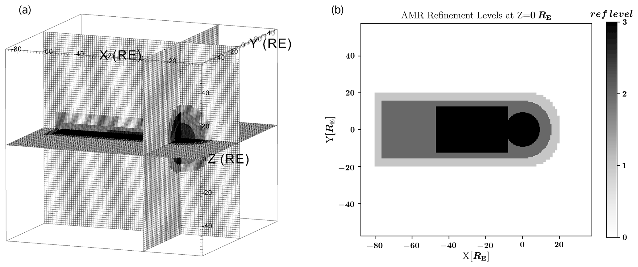
Figure 1 (a) Perspective 3D view of the AMR Vlasov grid. Here, the Earth is located at the axes' origin. (b) Equatorial distribution of the AMR refinement levels on the Vlasov grid in a 3D AMR simulation. Refinement level n corresponds to 2ⁿ times the base resolution. Darker regions closer to the Earth (n=3) are solved with the highest spatial resolution used in the simulation.

2.1 Grid coupling

DCCRG operates on a base refinement level, and each successive refinement level has twice the resolution of the previous one. At the highest refinement region there is a one-to-one match between the field solver and DCCRG's cells. However, the electromagnetic fields and plasma propagation are inherently dependent upon each other; thus, a coupling process takes place during every simulation time step. The coupling scheme is illustrated in Fig. 2. The Vlasov solver at the end of every time step feeds moments into the field solver grid. In regions where the one-to-one match is not fulfilled, one set of moments is communicated to all FsGrid cells which occupy the same volume as the underlying DCCRG cell. The field solver then propagates the fields and communicates those back to the Vlasov solver before the next time step begins. In mismatching regions, the field solver grid is fed uniform input in all the cells that are children of a lower-resolution DCCRG cell, and the parent DCCRG cell is later fed an averaged value of all the higher-resolution corresponding FsGrid cells. The association between the two grids is calculated during the initialization and after every load-balancing operation where the Cartesian spatial decomposition scheme over different MPI tasks changes for the DCCRG grid. When no AMR is used, the two solvers operate on the same spatial resolution; thus, there is a one-to-one grid match, making the coupling scheme trivial.

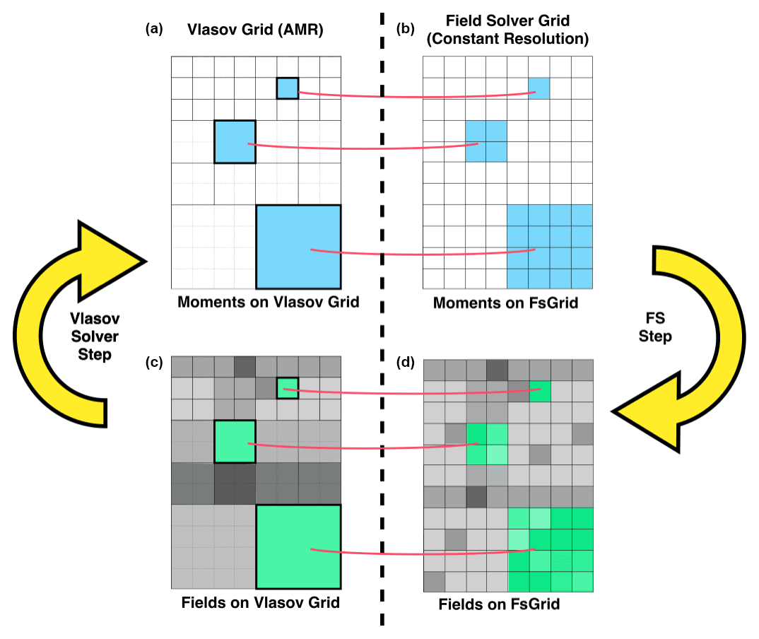
Figure 2 Schematic of the grid-coupling procedure. Moments evaluated on the Vlasov grid are copied over to the FsGrid. (a, b) When there is a grid mismatch, one DCCRG cell copies over its values to many FsGrid cells. Then the fields are propagated and finally fed back to the Vlasov grid. (c, d) In areas where the grids mismatch, multiple FsGrid cells are averaged to get the value for the corresponding DCCRG cell.

2.2 Staircase effect

In 6D AMR simulations, the one-to-one grid matching is restricted to only the highest refinement regions where both solvers operate at the highest spatial resolution. In less-refined regions, the Vlasov solver cells span multiple field solver cells and the grids mismatch. If the trivial coupling scheme described in the previous subsection is maintained, the field solver is subject to discontinuous plasma moment input at the Vlasov grid cell interfaces, which can be seen in Fig. 3a and b, as an effect that we dub the “staircase effect”. The discontinuities caused by the staircase effect lead to the development of unphysical oscillations in the field quantities on the field solver grid. The oscillations can be observed in the profiles demonstrated in Fig. 3d and f. Those oscillations can act as a source of spurious wave excitation and propagate artifacts in the whole simulation domain, as visible in Fig. 3c and e, where artifacts have propagated downstream from the bow shock of the global magnetospheric simulation, causing significant distortion of the physics in the nightside magnetosheath and lobes.

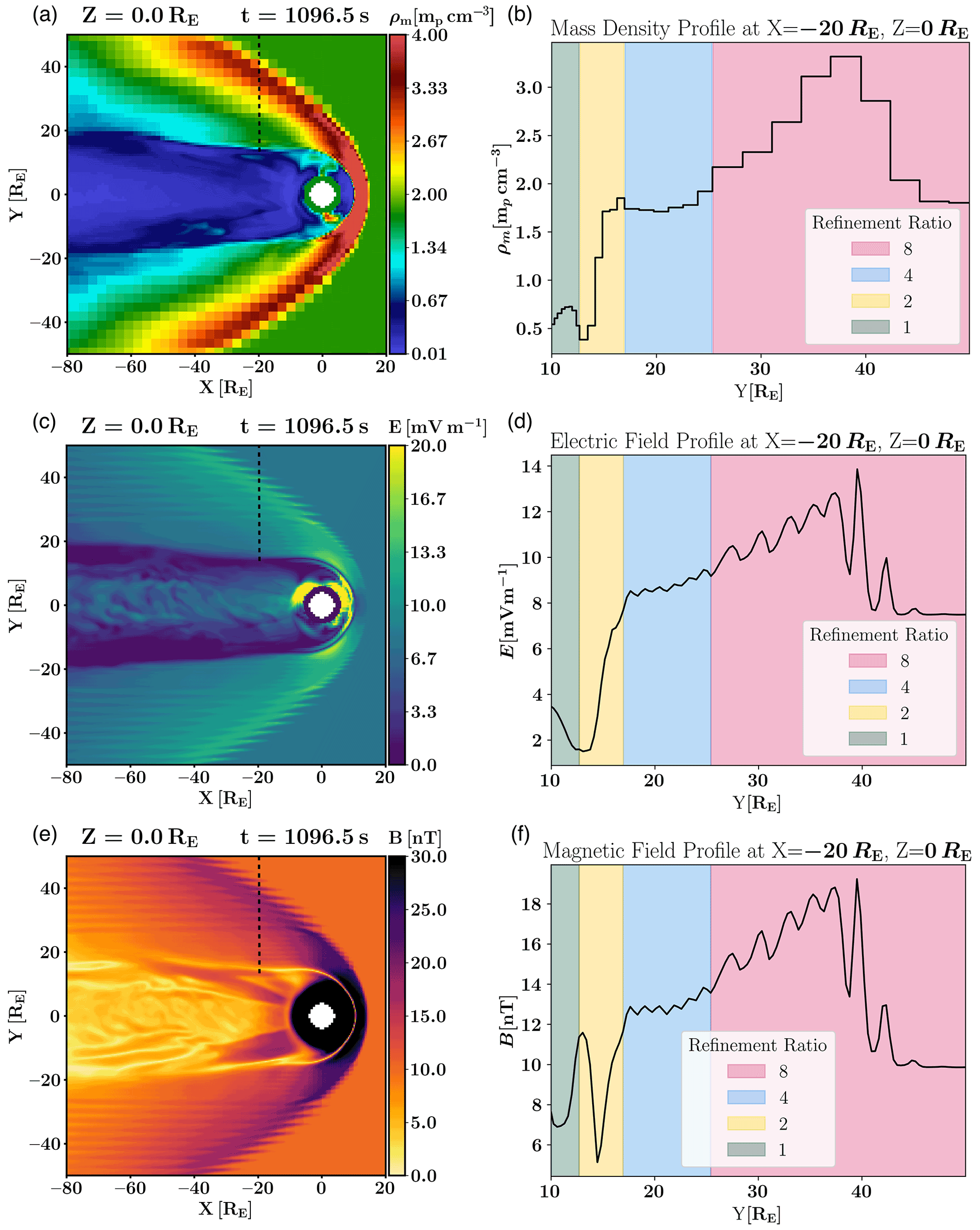
Figure 3 Visualization of a 6D Vlasiator simulation with heterologous grids. (a) Equatorial color map of mass density (on the AMR Vlasov grid). (b) Mass density along the profile shown as a dashed line in panel (a). In panels (a) and (b), m_p stands for proton mass. (c) Electric field magnitude color map (on the uniform FsGrid). (d) Electric field magnitude along the profile shown as a dashed line in panel (c). (e) Magnetic field magnitude color map (on the uniform FsGrid). (f) Magnetic field magnitude along the profile shown as a dashed line in panel (e). The colored regions in panels (b), (d), and (f) correspond to the resolution ratio between the field solver grid and the Vlasov grid. Unphysical oscillations in the field quantities, triggered by discontinuities in the moments, can be observed in the green and red regions.

3 Method

3.1 Low-pass filtering

Low-pass filtering is a well-known tool from digital signal processing theory that effectively attenuates unwanted high-frequency parts of the spectrum. The boxcar filter is the simplest finite impulse response low-pass filter, and it smooths out a signal by substituting a value with the average of itself and its two closest neighbors. Boxcar filters are usually cascaded with other boxcars in an attempt to reduce the high side lobes in their frequency response (Roscoe and Blair, 2016). Techniques like low-pass filtering are not limited to the time domain; they can be applied to other dimensions like ordinary space and find wide application in fields like image processing (Cook, 1986) and numerical modeling (Vay and Godfrey, 2014).

3.2 Spatial filtering

In this work, we present two implementations of the spatial filtering operator used in Vlasiator to smooth out the discontinuities in AMR simulations that are illustrated in Fig. 3a and b. First, in Vlasiator 5.1, the filtering operator is realized by a 3D 27-point (3 points per spatial dimension) boxcar kernel with equally assigned weights. The kernel operates in position space (r) and is passed over the field solver grid cells immediately after the coupling process finishes transferring Vlasov moments to the field solver grid. The filtering operator is only applied when there is a grid mismatch between the two solvers, so it is not used in the highest refinement level where the two solvers operate at the same spatial resolution. The number of times that the operator is applied is not constant but linearly depends on the refinement ratio between the two grids. Each filtering operator pass attenuates the high-frequency signals on the field solver grid and smooths out the discontinuities shown in Fig. 3a and b. Larger refinement ratios between the two grids give rise to spatially larger discontinuities, requiring more filtering passes in order to smooth the discontinuity. In practice, treating the finest to coarsest levels with 0, 2, 4, and 8 passes of the boxcar kernel, for example, has proved to alleviate the discontinuities illustrated in Fig. 3a and b.

At the end of each pass of the filtering scheme, a ghost cell communication update is required for the respective FsGrid structure prior to continuing on to the next pass. This manifests as a performance penalty, as the ghost communication is a global process involving all MPI tasks in the simulation. From the associative properties of the convolution operation, where B is a boxcar kernel, g is a function, and ⊛ is the convolution operator, we define the triangle kernel T, where

$$\begin{array}{}\text{(6)}& g⊛T=g⊛(B⊛B)=(g⊛B)⊛B.\end{array}$$

Two boxcar passes are the equivalent of a single triangular kernel pass; therefore, in Vlasiator 5.2.1, we update our filtering operator to a 3D 125-point triangle kernel. We choose the 3D triangle kernel as the convolution of a boxcar kernel with itself to match the frequency characteristics of the boxcar operator in half the number of passes, as shown in Fig. 4. The triangle kernel is used in the same fashion as the boxcar kernel; however, as half the number of passes per refinement level are required to achieve the same amount of smoothing this time, the triangular kernel operator performs half the amount of ghost cell communications. A graphical representation of the filtering kernels is given in Fig. 5. In Algorithm 1, we demonstrate the two implementations of the spatial filtering algorithm with a 1D pseudo-code example. The modified coupling scheme is demonstrated in Fig. 6, where it is now supplemented with the filtering mechanism, in contrast to Fig. 2.

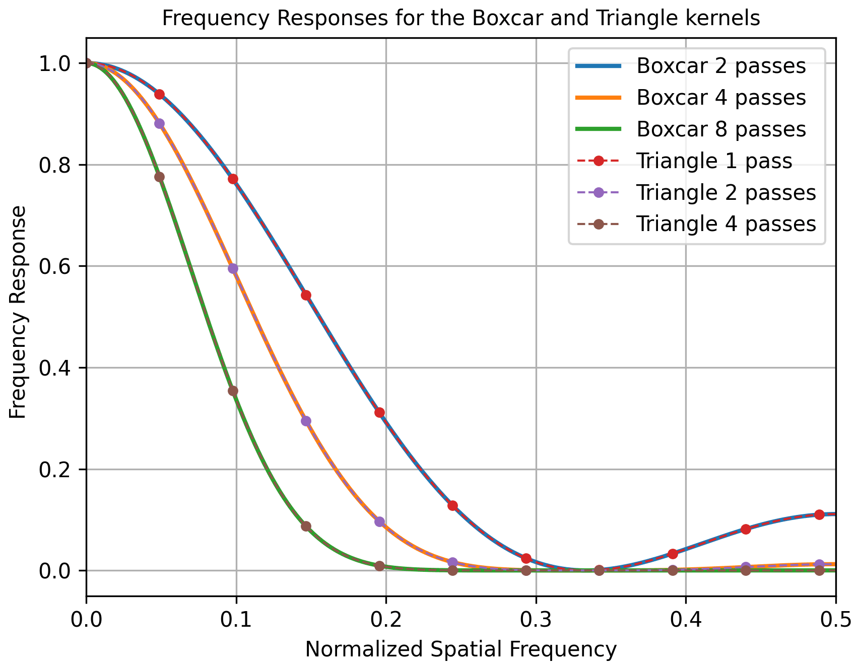
Figure 4 Solid lines show the frequency response of the boxcar filter operator for different numbers of passes as used in Vlasiator. Dashed lines show the frequency response of the triangular filter operator for different numbers of passes as used in Vlasiator.

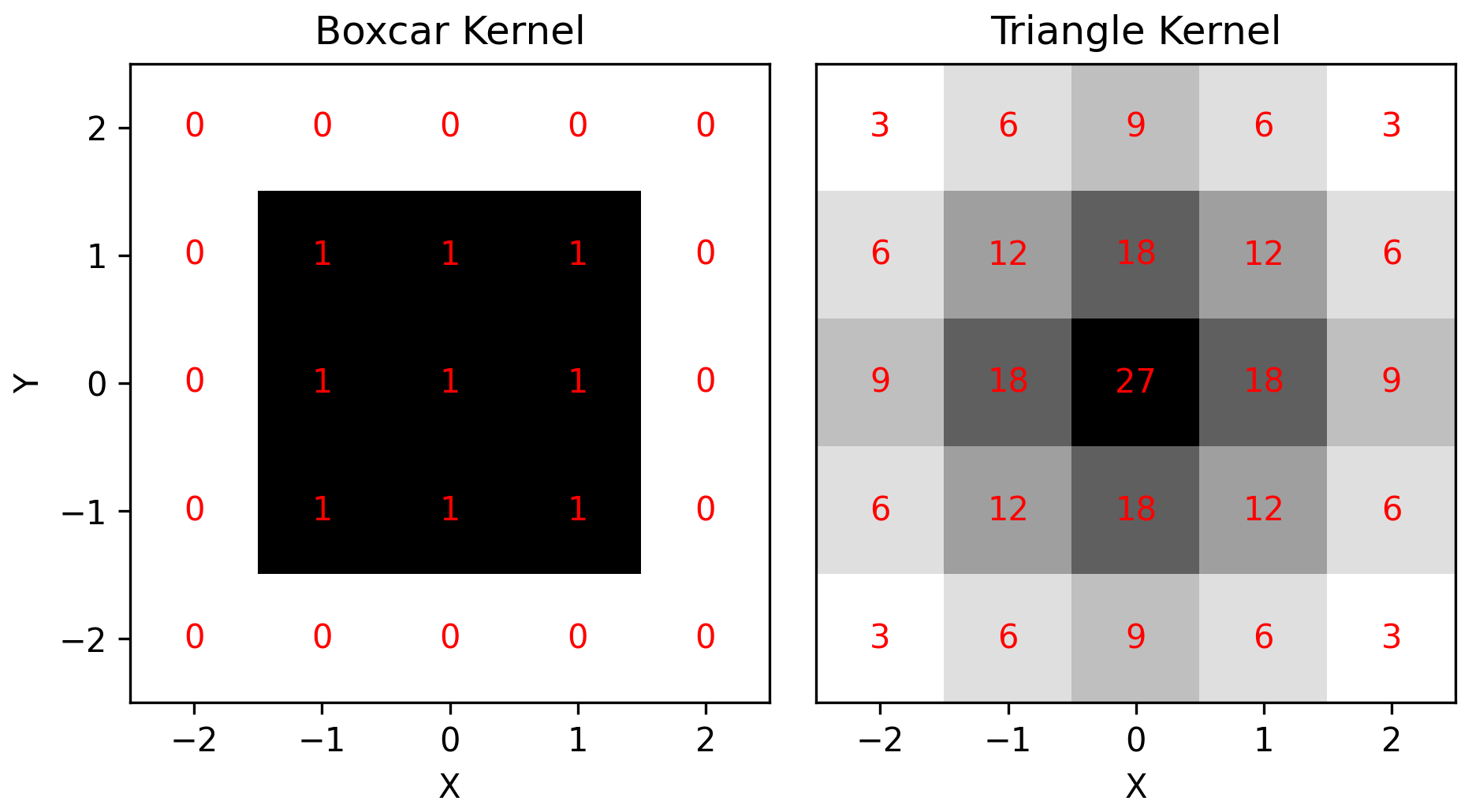
Figure 5 Graphical representation of the boxcar and the triangle kernels. The 2D slices are taken from the middle of the kernel's third dimension. For better clarity, the boxcar kernel is padded with zeros and the kernel weights, shown in red font, are not normalized.

Figure 6 Schematic of Vlasiator's grid-coupling scheme supplemented with the extra filtering step to alleviate the staircase effect in 6D AMR runs.

Algorithm 1 Filtering operator pseudo-code

1:

if method==”boxcar” then

2:

kernelWidth←1

3:

$kernelWeights\leftarrow [\mathrm{1},\mathrm{1},\mathrm{1}]$

4:

sum←sum(kernelWeights)

5:

else if method==”triangle” then

6:

kernelWidth←2

7:

$kernelWeights\leftarrow [\mathrm{1},\mathrm{2},\mathrm{3},\mathrm{2},\mathrm{1}]$

8:

sum←sum(kernelWeights)

9:

end if

10:

swapGrid←momentsGrid

11:

for $pass=\mathrm{0},\mathrm{1},\mathrm{\dots }maxPasses$ do

12:

for $i=\mathrm{0},\mathrm{1},\mathrm{\dots }momentsGrid.GridSize$ do

13:

$refLevel\leftarrow momentsGrid.getRefLevel\left(i\right)$

14:

if pass>=momentsGrid.numPasses(refLevel) then

15:

continue

16:

end if

17:

swapGrid[i]←0.0

18:

for $j=-kernelWidth\mathrm{\dots }kernelWidth$ do

19:

$ii\leftarrow i+j$

20:

$swapGrid\left[i\right]+=momentsGrid\left[ii\right]*kernelWeights[kernelWidth+j]/sum$

21:

end for

22:

end for

23:

momentsGrid←swapGrid

24:

momentsGrid.updateGhostCells()

25:

end for

4 Results

To demonstrate the effect of the spatial filtering employed in Vlasiator 5.1 to alleviate the AMR discontinuities, we create a simple configuration with a density step in the middle of a 3D simulation box. The step, shown in Fig. 7, poses a discontinuity in the otherwise smooth mass density. Similar steps are created during AMR simulations in regions where there is no one-to-one match between the Vlasov and field solver grid cells. We apply the boxcar filtering operator an increasing number of times to evaluate its performance, and the results are illustrated in Fig. 7. When the filtering operator is cascaded with itself, its effect becomes more significant in damping high-frequency signals, as shown in Fig. 4. In Fig. 7, we only show the effect of the boxcar operator because the results are identical to using the triangular kernel operator, as shown by the frequency response of the two kernels depicted in Fig. 4.

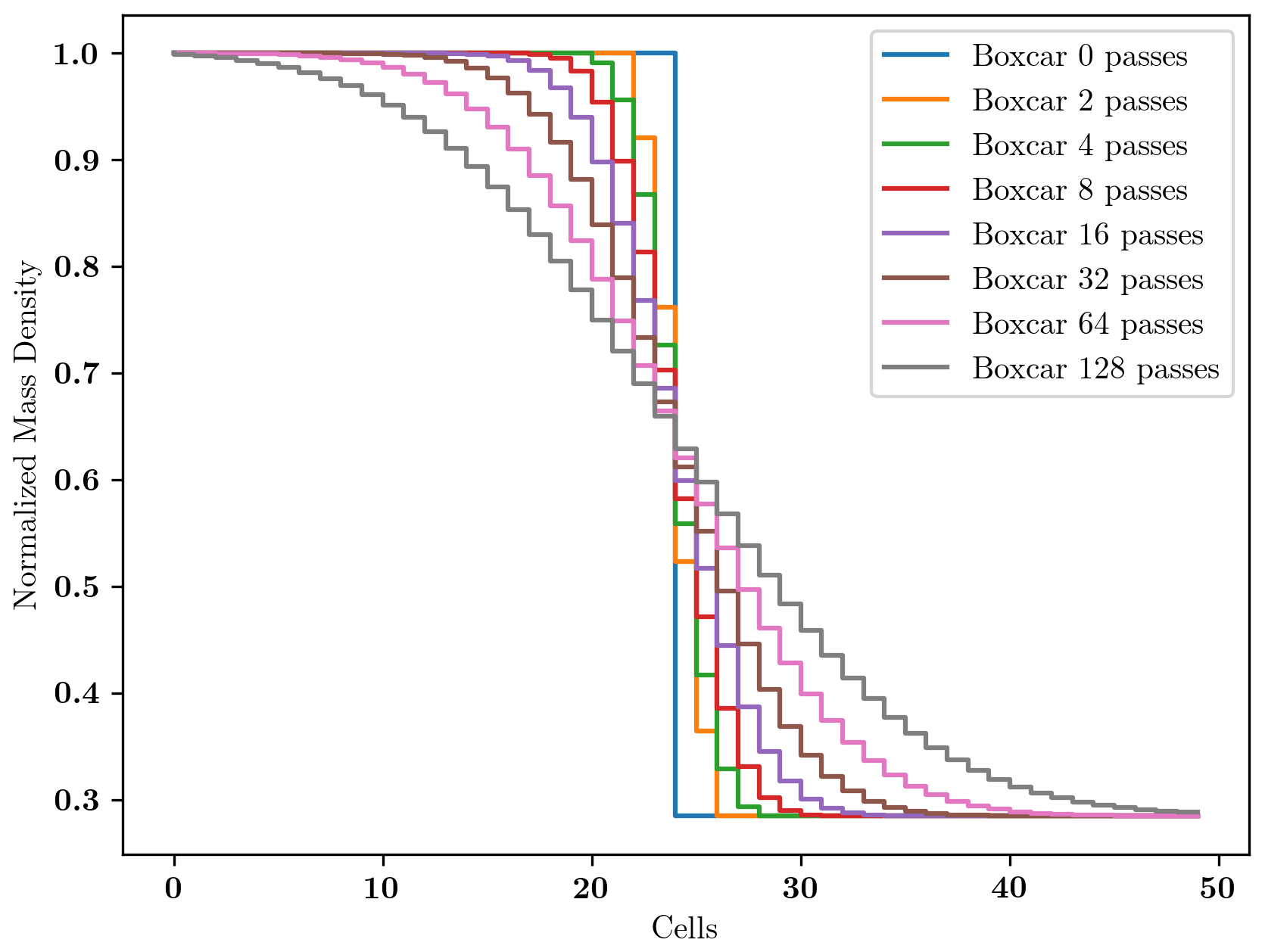
Figure 7 Smoothing of a step in mass density along a line in the simulation domain intersecting a discontinuity. The unfiltered normalized mass density line profile is shown in blue, and the other colors correspond to an increasing number of boxcar passes.

Furthermore, we demonstrate the results of the boxcar filtering operator in a large magnetospheric production-scale run using four AMR levels. Simulation quantities on the heterogeneous grid structure are illustrated in Fig. 8. In Fig. 8a, a color map of the mass density on the AMR Vlasov grid is depicted. The discontinuities at the AMR level interfaces are visible. In Fig. 8b, a color map of the mass density on the uniform field solver grid is illustrated after the coupling process has taken place. During the coupling process, the filtering operator is used, and the AMR levels are treated, from finest to coarsest, with 0, 2, 4, and 8 passes, respectively. Figure 8c and e show the respective electric field and magnetic field magnitudes simulated with filtered moments on FsGrid. The profiles demonstrated in Fig. 8d and f are sampled along the dashed paths in Fig. 8c and e, respectively.

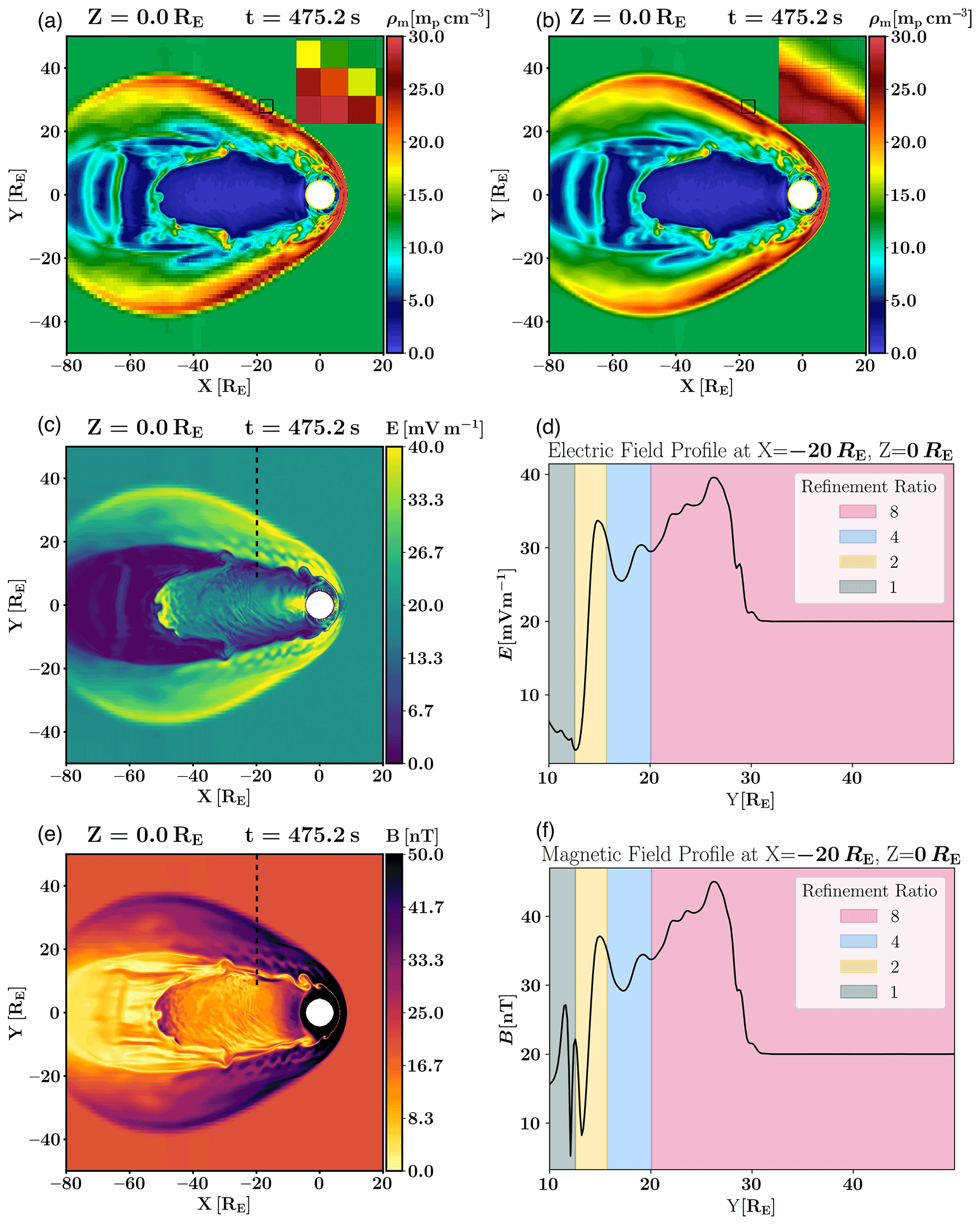
Figure 8 Vlasiator magnetospheric simulation results. (a) Mass density color map (on the AMR Vlasov grid) of a 6D AMR simulation. (b) Mass density color map (on the uniform FsGrid) of a 6D AMR simulation with the filtering operator in use. In panels (a) and (b), m_p stands for proton mass. There are four refinement levels, and they are treated with 0, 2, 4, and 8 filtering passes from finest to coarsest, respectively. The insets in panels (a) and (b) illustrate the mass density on the uniform field solver grid. The AMR Vlasov mesh is denoted by the black lines. The insets are taken from the regions highlighted by black squares in panels (a) and (b). The step discontinuities visible in the inset in panel (a) are spatially co-located with the DCCRG grid cells. (c) Electric field magnitude color map (on the uniform FsGrid) with the filtering operator in use. (d) Electric field profile sampled along the dashed line in panel (c). (e) Magnetic field magnitude color map (on the uniform FsGrid) with the filtering operator in use. (f) Magnetic field profile sampled along the dashed line in panel (e).

The simulation used to evaluate the filtering operator models a 3D space around Earth in the Geocentric Solar Magnetic (GSM) coordinate system with no dipole tilt. The modeled space extends from −560 000 to 240 000 km in the X dimension, from −368 000 to 368 000 km in both the Y and Z dimensions, and is represented by a $\mathrm{100}\times \mathrm{92}\times \mathrm{92}$ Cartesian mesh with Δr=8000 km at the lowest refinement level and with Δr=1000 km at the highest refinement level. Each spatial cell contains a velocity space with a 3D grid with $\mathrm{\Delta }v=\mathrm{40}\mathrm{km}{\mathrm{s}}^{-\mathrm{1}}$. The solar wind is modeled with proton density $n=\mathrm{7}{\mathrm{cm}}^{-\mathrm{3}}$, temperature $T=\mathrm{0.5}\times {\mathrm{10}}^{\mathrm{6}}\mathrm{K}$ and solar wind speed $V_x=-\mathrm{1000}\mathrm{km}{\mathrm{s}}^{-\mathrm{1}}$. The interplanetary magnetic field points mostly southward with $\mathit{B}=[-\mathrm{0.5},\mathrm{0},-\mathrm{20}]\mathrm{nT}$.

4.1 Performance overhead

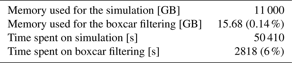
Care has to be taken to keep the performance overhead of the filtering operator small. The boxcar operator is applied at every simulation time step and makes use of a duplicate FsGrid structure of the Vlasov moments because the filtering cannot happen in place. The boxcar operator uses OpenMP threading to parallelize the filtering over the local domain of each MPI task. In Table 1, we report the extra memory needed for the filtering operator and the time spent filtering the Vlasov moments during the grid-coupling process for the production 6D AMR run shown in Fig. 8.

From Table 1, we see that the boxcar filtering operator used in Vlasiator 5.1 amounts to 6 % of the total simulation time for a production run like the one in Fig. 8. To evaluate the performance improvement of the five-stencil triangle kernel implementation, used in Vlasiator 5.2.1, we set up smaller tests and compare the two methods. The triangle kernel operates in the same way but only needs half the numbers of passes to achieve proper smoothing, so we treat the finest to coarsest levels with 0, 1, 2, and 4 passes. We report the results in Table 2.

Table 1 Profiling statistics for the boxcar filtering operator.

Table 2 Comparison of the two filtering kernels' performance.

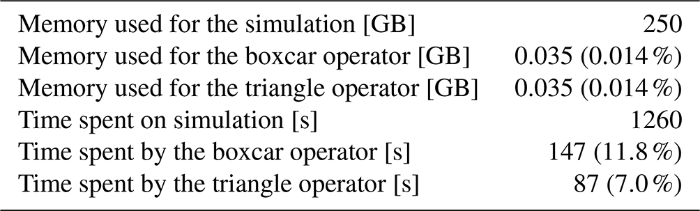
While both approaches require the same amount of memory, the time spent by the triangular operator amounts to 59 % of that spent by the boxcar operator.

Both the boxcar and the triangular filtering operators are 3D spatial convolutions that can be expressed as three 1D convolutions (Birchfield, 2017). This is known as kernel separability and can improve the performance of the two operators significantly. Formally, the use of a separable kernel instead of a 3D one, would reduce the complexity from $\mathcal{O}(N_x\times N_y\times N_z\times d^{\mathrm{3}})$ (where $N_x,N_y,$ and N_z are the dimensions of the simulation mesh, and d is the dimension size of the 3D kernel) to $\mathcal{O}(\mathrm{3}\times N_x\times N_y\times N_z\times d)$. We modify our implementations of the 3D boxcar and triangle operators to take advantage of the kernel separability property and test their performance using the same configuration used to produce the results in Table 2. We demonstrate the performance statistics of all four methods in Fig. 9.

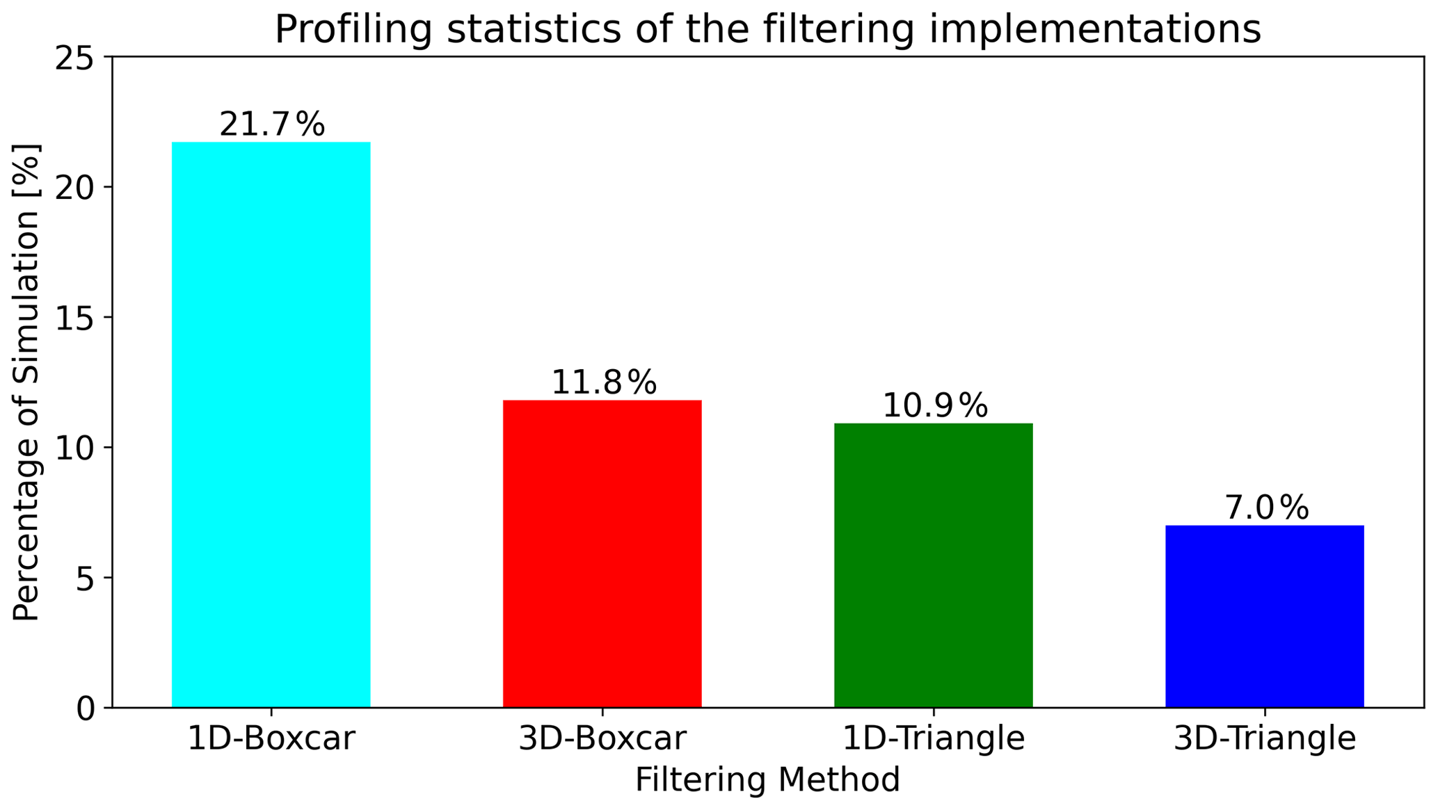
Figure 9 Profiling statistics for the different implementations of the filtering operators in Vlasiator. The results are derived from a custom simulation setup designed to test filtering performance.

While the separable operators should theoretically lead to a significant performance gain, the 1D operators are slower than their 3D counterparts in practice. This is due to the fact that an interim ghost-update communication needs to take place after every pass done by the operators, and, as the 1D implementations require more mesh traversals per pass, they end up spending more time on updating their ghost cell values. Additionally, we note that kernel separability does not hold if the stencil is altered – for example, when part of the kernel covers the highest refinement level.

4.2 Moment conservation

The filtering operator, as described above, is not conservative at the interface of adjacent refinements levels. However, this is not a cumulative effect because moments on FsGrid, used to propagate the electromagnetic fields, are provided to the field solver by the Vlasov solver at each time step and are not copied back from the FsGrid. Furthermore, the moment conservation is also violated due to numerical precision round-off errors during the filtering passes. The amount by which the moments are not conserved depends on the number of filtering passes and on the number of cells in a given simulation. We measure the relative difference in mass density caused by the filtering operator in the simulations presented in this work and find it to always remain below 10⁻⁵, which we deem acceptable given the non-cumulative nature of the filtering operation.

5 Discussion

The first 6D simulations with Vlasiator 5.0 would not have been possible without the use of AMR. However, the heterologous grid structure and the grid-coupling mechanism in Vlasiator create artifacts in simulations using AMR that alter the global physics. In this work, we report on a new development employing spatial filtering in the hybrid-Vlasov code Vlasiator (versions 5.1 and 5.2.1) in order to alleviate the staircase effect created due to the heterologous AMR scheme used in 6D simulations. Based on the results of this study, the use of a linearly increasing number of passes per refinement level minimizes the aliasing effect at the Vlasov–field solver grid interfaces. Treating the finest to coarsest levels with 0, 2, 4, and 8 passes of the boxcar filter, for example, has proved to alleviate the staircase effect satisfactorily, as can be seen in Fig. 8a and b. As a result, the electric and magnetic field magnitude profiles in Fig. 8d and f show none of the oscillatory behavior caused by the staircase effect, in contrast to those demonstrated in Fig. 3d and f. As the filtering operator is applied at every simulation time step, it has to be well optimized so that it does not increase the computational overhead significantly. From Table 1, we see that the filtering in a production simulation amounts to 6 % of the computational time, which we deem significant. To improve the filtering performance, we develop a 3D five-point stencil triangle kernel in Vlasiator 5.2.1, which is equivalent with respect to alleviating the staircase effect but only needs half the number of passes per refinement level. We test the triangle kernel on a smaller simulation and report on its performance in Table 2. The triangle kernel provides a 41 % performance improvement over the boxcar approach; thus, we estimate that, in a similar simulation to the one shown in Fig. 8 it would amount to 3.5 % of the total simulation time, which we deem acceptable. The improved performance is a combination of both halving the ghost cell updates needed for the triangular kernel operator and reducing the operations needed because the wider kernel operator requires half the number of passes compared with the boxcar operator. Furthermore, we evaluate the performance gain acquired by exploiting the filter separability property of the two filtering operators and conclude that the separable kernels in fact perform worse in the context of Vlasiator than their 3D counterparts, as they are hindered by the higher number of ghost cell updates that they require. Another approach to improve the performance of the filtering methods would be to use an even wider kernel to completely eliminate the ghost cell updates; however, that would require increasing the number of ghost cells used by FsGrid. We choose to limit the number of ghost cells to four per dimension (two ghost cells per side) to avoid the extra memory penalty; thus, we limit ourselves to using five-point stencils. A larger ghost domain would also make existing ghost communication more expensive. Furthermore, the memory footprint is the same for both methods and insignificant compared with the memory needed to store the velocity distribution function for each spatial cell, as shown in Table 1. The filtering operator presented in this work has been used to aid in 6D simulations performed with Vlasiator with respect to efficiently alleviating the artifacts introduced by the staircase effect.