the Creative Commons Attribution 4.0 License.
the Creative Commons Attribution 4.0 License.
 | 24 Oct 2022
Development of a regional feature selection-based machine learning system (RFSML v1.0) for air pollution forecasting over China
Li Fang
Arjo Segers
Hai Xiang Lin
Mijie Pang
Cong Xiao
Tuo Deng
Hong Liao
With the explosive growth of atmospheric data, machine learning models have achieved great success in air pollution forecasting because of their higher computational efficiency than the traditional chemical transport models. However, in previous studies, new prediction algorithms have only been tested at stations or in a small region; a large-scale air quality forecasting model remains lacking to date. Huge dimensionality also means that redundant input data may lead to increased complexity and therefore the over-fitting of machine learning models. Feature selection is a key topic in machine learning development, but it has not yet been explored in atmosphere-related applications. In this work, a regional feature selection-based machine learning (RFSML) system was developed, which is capable of predicting air quality in the short term with high accuracy at the national scale. Ensemble-Shapley additive global importance analysis is combined with the RFSML system to extract significant regional features and eliminate redundant variables at an affordable computational expense. The significance of the regional features is also explained physically. Compared with a standard machine learning system fed with relative features, the RFSML system driven by the selected key features results in superior interpretability, less training time, and more accurate predictions. This study also provides insights into the difference in interpretability among machine learning models (i.e., random forest, gradient boosting, and multi-layer perceptron models).
- Article
(6049 KB) - Full-text XML
- Companion paper
-
Supplement
(43936 KB) - BibTeX
- EndNote


With ongoing economic development and modern industrialization, the subsequent air pollution poses serious threats to resident health (Liu and Diamond, 2005; Li et al., 2014). After tobacco and high blood pressure, air pollution has ranked third in risk factors for death and disability in China over the past few decades (Murray et al., 2020). The primary air pollutants in China are particulate matter (PM), sulfur dioxide (SO2), carbon monoxide (CO), nitrogen oxides (NOx) and ozone (O3) (Song et al., 2017b). PM2.5 or respirable PM in air with an aerodynamic diameter below 2.5 µm is the primary air pollutant, and it has attracted considerable attention from researchers (Zhai et al., 2019). Exposure to either long-term or short-term PM2.5 is related to respiratory symptoms, lung disease, cardiovascular disease, premature death, and other adverse health effects (Pui et al., 2014; Di et al., 2019). Burnett et al. (2018) and Song et al. (2017a) reported that PM2.5 pollution in winter, particularly in northern China, is severe. It accounted for 15.5 % (1.7 million) of all deaths in China in 2015, despite an improvement in air quality since 2013. In recent studies, the global exposure mortality model has estimated that 140 200 premature deaths from 2015 to 2019 can be attributed to long-term exposure to PM2.5 (Hao et al., 2021). An accurate air quality forecast (e.g., forecasting PM2.5) is therefore valuable to policy makers and health professionals for epidemiological control (Xue et al., 2019). In addition, it can provide an early warning for residents, particularly for children, the elderly, and people with respiratory or cardiovascular problems (Hu et al., 2017).
The development of an air pollution forecasting model is possible, as atmospheric chemistry and physical rules have been explored and are now understood in depth (Sun and Li, 2020b). In addition, our ever-increasing computational power can support the complex and heavy computational tasks required for this type of model (Reichstein et al., 2019). Deterministic models, such as chemical transport models (CTMs), and data-driven methods are commonly employed in forecasting (Cobourn, 2010; Xu et al., 2021). In several studies, air pollution forecasting has been performed using mainstream air quality CTMs, such as the Weather Research and Forecasting model with Chemistry (Grell et al., 2005; Zhou et al., 2017), Community Multiscale Air Quality model (Liu et al., 2018), and GEOS-Chem (Bey et al., 2001; Jeong and Park, 2018). These CTMs can reproduce real atmospheric situations (Hutzell and Luecken, 2008; Shtein et al., 2020); however, they exhibit several shortcomings. One of the most difficult setbacks is the high uncertainty in emission inventories (Huang et al., 2021), which is a great challenge given the variety of contributing sources, complexity of the spatial–temporal profiles, and lack of reliable in situ measurements (M. Li et al., 2017). Additionally, an idealistic deterministic model requires a delicate and thorough understanding of physical and chemical processes in the atmosphere (Sun and Li, 2020a) and an enormous computational capacity to resolve fine-scale variabilities. Therefore, CTMs alone have failed to meet the requirements for an effective air quality early warning system.
In contrast to CTMs, data-driven methods that do not require a profound knowledge of the complex composition or structure of the atmosphere are also widely utilized in atmospheric modeling (Ziomas et al., 1995; Xi et al., 2015). Many of these methods have been employed for air pollution forecasting, including multiple linear regression (Sawaragi et al., 1979), nonlinear regression models such as principal component regression (Shishegaran et al., 2020), hidden Markov models (Sun et al., 2013), support vector machine (Abu Awad et al., 2017), and artificial neural networks (Fernando et al., 2012). Of these methods, machine learning models have gained the greatest popularity because of their capacity to learn complex and nonlinear relationships by assimilating “big” training datasets (Masih, 2019; Leufen et al., 2021). Machine learning has brought great opportunities and challenges to the geophysical research community (Yu and Ma, 2021).
With the explosive growth of data in earth science, the superiority of machine learning for massive data applications has become increasingly prominent (Reichstein et al., 2019). The most representative example is to perform predictions for a target site using a machine learning model trained via a long-term series of in situ historical measurements. The China Ministry of Environmental Protection (MEP) has established many ground-based stations measuring the primary pollutants since 2013 (Zhai et al., 2019). At present, the monitoring network comprises more than 1500 field stations covering all of China, as can be seen in Fig. 1. The richness of air quality observations from the monitoring network provides valuable training data and stimulates the development of machine learning air quality forecasting in China (Xu et al., 2021). Previous studies on air pollution forecasting in China have utilized various machine learning models with the ground-based MEP air quality dataset. For example, X. Li et al. (2017) utilized a long short-term memory (LSTM) neural network extended model to predict PM2.5 concentrations at a maximum forecast horizon of 24 h for air quality monitoring stations in Beijing, China. Wu et al. (2020) proposed a composite prediction system based on an LSTM neural network to predict daily PM2.5 PM10 in Wuhan. Zhang et al. (2020) established a hybrid model, integrating deep learning with multi-task learning, to predict hourly PM2.5 concentrations in three different districts of Lanzhou. Ke et al. (2021) utilized four machine learning models to develop an air quality forecasting system that can automatically find the best model and hyperparameter combination for the next 3 d air quality forecast in seven megacities of China. These works are highly valuable in exploring novel methods of air quality prediction relative to conventional CTMs. To the best of our knowledge, the aforementioned studies on air pollution forecasting solely focused on a few monitoring stations, typical cities, or small regions, while national-level air quality predictions remain lacking. The challenges in national-level forecasting include substantial temporal and spatial variances (Song et al., 2017b) in air pollution and enormous computational power requirements.
The curse of dimensionality is a common obstruction in modeling; i.e., an increasing amount of input data leads to rapidly increasing complexity, and prediction algorithms are susceptible to over-fitting (Rodriguez-Galiano et al., 2012). Therefore, considerable research has focused on reducing the dimensionality of input data by selecting only significant variables and eliminating redundancy. The methods of this research can be classified into three categories: the filter method (e.g., a correlation matrix using the Pearson Correlation), wrapper method (e.g., recursive feature elimination), and embedded method (e.g., Lasso regularization) (Chandrashekar and Sahin, 2014). These methods can reduce the adverse effects of irregular variables or noise while retaining prediction performance (Guyon and Elisseeff, 2003). They also save computing resources for model training. However, in previous studies on air quality forecasting, filter methods such as Pearson correlation coefficients or the maximal information coefficient (MIC) (Kinney and Atwal, 2014) were commonly utilized for input selection. These input selection methods can help improve the performance of machine learning models; however, they all have serious limitations. For example, universal meteorological variables that highly correlate with PM2.5 in a large region of China are difficult to find using Pearson correlation coefficients because they can vary substantially both spatially and temporally (Zhai et al., 2019). MIC is the most employed method for capturing linear and nonlinear correlations between variable pairs (Chen et al., 2016). However, it cannot consider relevance and redundancy simultaneously (Sun et al., 2018). Furthermore, MIC is computationally intensive (Cao et al., 2021).
Machine learning algorithms are often considered “black box” models that learn the input–output relationship from immense training samples (Casalicchio et al., 2019). Many researchers have devoted enormous efforts to developing and implementing tools to interpret machine learning models. Among these tools, game-theoretic formulations of feature significance are the most widely utilized because they can capture the interactions among features (Shapley, 1952), and they may be the only solution satisfying the four “favorable and fair” axioms (Fryer et al., 2021). Several scholars have conducted in-depth studies on distinguishing feature significance based on the Shapley value (Shapley, 1952). For example, Park and Park (2021) utilized the Shapley additive explanation (SHAP) approach (Lundberg and Lee, 2017a) to interpret multiple machine learning models and found that most of the models have similar features. Golizadeh Akhlaghi et al. (2021) successfully interpreted the feature contributions of the guideless irregular dew-point cooler on the predicted parameters based on SHAP. In addition to SHAP, which explains individual predictions, Covert et al. (2020) proposed a novel method that can explain model behavior across the entire dataset (global interpretability), called Shapley additive global importance (SAGE). SHAP and SAGE both utilize the Shapley value; however, compared with SHAP, SAGE can simultaneously eliminate larger subsets of redundant features (Covert et al., 2020). Additionally, SAGE extracts features from the conditional distribution instead of the marginal distribution because the latter may lead to breaking feature dependencies and producing unlikely feature combinations (Lundberg and Lee, 2017a). Furthermore, investigating the feature importance based on model performance (Jothi et al., 2021) has been verified as a meaningful and effective approach for interpreting data-driven models and is popular in computer science (Altmann et al., 2010). However, this method has rarely been applied to air quality forecasting using machine learning tools.
In the present study, the first version of a regional feature selection-based machine learning system (RFSML v1.0) is developed. The system can predict short-term air quality with high accuracy in China. In this study, the RFSML system predicts the primary air pollutant (PM2.5) concentration over every target site from the China MEP air quality monitoring network by learning its implicit trend from long-term series records. This method can be extended to other airborne pollutant predictions in future studies. SAGE analysis is adopted to interpret valuable features and exclude redundant inputs to avoid over-fitting the model during training. Because the SAGE calculations are more time-consuming than the model training, as explained in Sect. 3.1, they are not repeated for every target site but are implemented in limited ensemble sites that are randomly selected in a given region. China was divided into five densely populated regions, according to the air pollution patterns, which are consistent with the Clean Air Action target regions released by the Chinese State Council, as discussed in Sect. 2.2.3. The top three critical features in the ensemble SAGE calculations were utilized as the input features for the implicit trend model training for each site. The robustness of the regional feature selection was tested over three widely utilized machine learning models, i.e., random forest (RF), gradient boosting (GB), and multi-layer perceptron (MLP) models, and four forecasting horizons (6, 12, 18, and 24 h).
The remainder of the paper is organized as follows: the composition of the data used in this study and the pre-processing method are introduced in Sect. 2. Then, the three machine learning models and their hyperparameter choices utilized in this study are described. The principles of SAGE and the details of the SAGE ranking-based regional feature selection are described at the end of Sect. 2. In Sect. 3, the computational costs of SAGE and machine learning model training are detailed. Then, the results of feature selection in each region are presented and analyzed. The prediction performance of RFSML is evaluated and compared with that of the standard machine learning process. Finally, the conclusions and future prospects are provided in Sect. 4.
The components of the RFSML method that are used to forecast PM2.5 concentrations are described in the following sections.
2.1 Model domain and data
The RFSML system forecasts air pollution levels in the vicinity of a monitoring station. This forecasting uses machine learning by examining the variability in the available station datasets. The monitoring network consisted of 1588 stations, for data collected in 2019, at the locations displayed in Fig. 1. Because the station network is dense, pollution-level forecasting can be performed for nearly any location in eastern China.
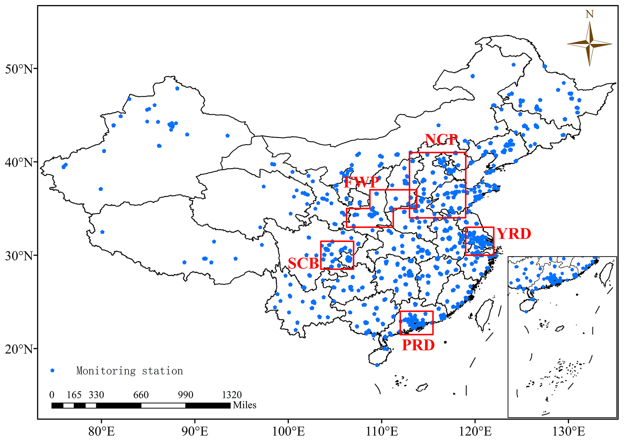
Figure 1Locations of environmental monitoring stations in the study area in 2019 (blue pentagons). Red rectangles represent the five primary megacity clusters in China.
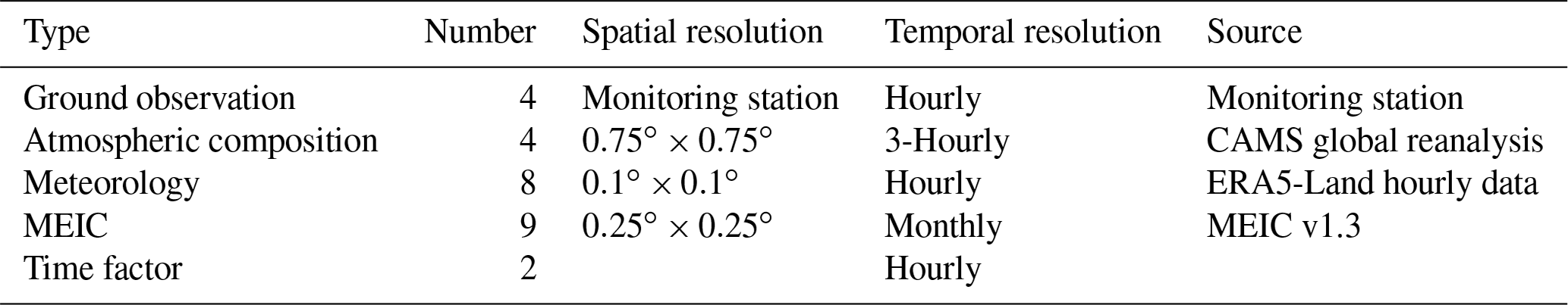
The input data for machine learning consisted of hourly averaged air pollutant measurements (e.g., PM2.5, CO, SO2, and NO2) from the Chinese MEP monitoring network, meteorological reanalysis data from ERA5-Land (Muñoz Sabater et al., 2021), atmospheric composition data from the Copernicus Atmosphere Monitoring Service (CAMS) reanalysis (Inness et al., 2019) provided by the European Centre for Medium-Range Weather Forecasts (ECMWF), and emission data from the Multi-resolution Emission Inventory for China (MEIC) inventory, with time factors applied at an hourly resolution. The input data are summarized in Table 1. The variables in the datasets are correlated with and may drive the PM2.5 concentration and are therefore useful predictors.
Data from 2018 and 2019 were used in the experiments. The first 15 690 h (from 1 January 2018 to 15 October 2019) was used for model training and cross-validation, and the actual tests were performed using the remaining 1824 h of data from 15 October to 30 December 2019. Our RFSML system can of course operate in a rolling way; additional forecasts in a less polluted period, April 2020, are performed with the models similarly trained using the recent 2-year data.
2.1.1 Air pollutant observations
The observed air pollutant concentrations at the stations were used as inputs (NO2, SO2, and CO) and target variables (PM2.5) in the model training. The available time series of PM10 observations was missing many values and was therefore excluded from the model. Additionally, O3 observations were excluded because these data exhibit a diurnal cycle that substantially differs from the PM2.5 target concentrations.
Missing data occurred for each of the studied pollutants because of equipment failure, incorrect sensor readings, and improper operation. For the PM2.5 time series, approximately 14.6 % of the observations were missing on average, as illustrated in Fig. 2a. However, an uninterrupted time series is necessary for model training and rolling forecasting. In studies such as Qin et al. (2019) and J. Ma et al. (2019), it was shown that the observations from surrounding monitoring stations can be utilized to insert suitable values for missing data through imputation. Data imputation tools, such as cubic interpolation, have gained popularity for enhancing monotone data (Fritsch and Carlson, 1980).
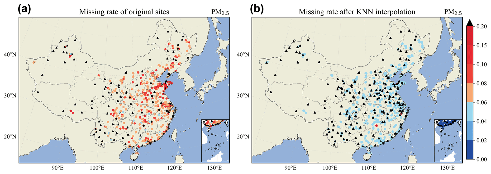
Figure 2Missing fraction of (a) original and (b) KNN-interpolated PM2.5 data. Dots and triangles denote the locations of air quality monitoring stations, and dot colors represent the missing data rate of each monitoring station. Black triangles indicate monitoring stations with 20 % missing data or over 15 % missing data after KNN interpolation that were excluded from the model.
In this study, the K-nearest neighbor (KNN) classification method (Zhang, 2012) and cubic imputation were combined to create an uninterrupted time series. The KNN algorithm is illustrated as Algorithm S1 in the Supplement. The KNN algorithm was implemented using the following steps:
-
Monitoring stations with over 20 % missing data were excluded from the training and prediction because such large amounts of missing data are not believed to be filled with sufficient accuracy.
-
For each station, the number of monitoring stations within a radius of 0.8∘ was calculated (following the empirical choices suggested in Jin et al., 2019). If fewer than three surrounding stations were available, the station was excluded from the training and forecasting. If three or four surrounding stations were found, these were all selected, while four stations were selected randomly if more than four surrounding stations were found.
-
For each target station, a geographic inverse distance weighting technique (Bartier and Keller, 1996) was used to estimate the missing values using the observed values from the surrounding stations.
After KNN interpolation, the amount of missing data in the PM2.5 time series was reduced to approximately 4.5 %, as illustrated in Fig. 2b.
Because there were cases where nearby stations and the target station simultaneously exhibited missing data, some instances of missing values remained after KNN interpolation. Therefore, cubic imputation (Kincaid et al., 2009) was employed to insert values for the remaining missing data. Outliers generated by the cubic imputation were replaced with the minimum or maximum of the original series. A total of 1263 monitoring stations exhibited no missing data after applying interpolation. Both the mean and standard deviation of the homogenized time series were similar to those of the original data, as illustrated in Fig. S1 in the Supplement.
2.1.2 Air pollutant forecast product and meteorological variables
The CAMS reanalysis (Inness et al., 2019) provides three-dimensional simulations of the atmospheric composition obtained by combining a global atmospheric chemistry model and observations. Therefore, it is expected to surpass pure model-based prediction accuracy. Selected concentrations of trace gases and aerosols from the CAMS reanalysis were inputs for the PM2.5 predictor. The PM2.5 simulations in this dataset were also used as a benchmark for the RFSML prediction.
We obtained the 3-hourly reanalysis data of four air pollutant concentrations (pm2p5, no2, so2, and co), which are reanalysis data (pm2p5, no2, so2, and co) of four ground observations mentioned above, in China from 2018 to 2019. The 3 h temporal resolution of the CAMS reanalysis data is firstly interpolated into 1 h resolution by cubic imputation. Then continuous time series of features at the monitoring stations are extracted from the interpolated 1 h data at a resolution of using the nearest mapping.
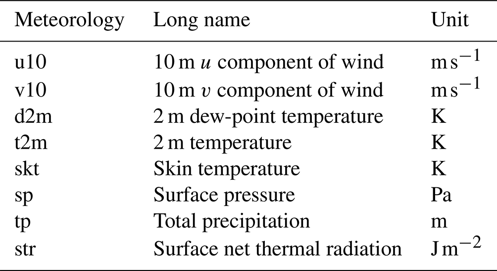
Meteorological variables, as illustrated in Table 2, were obtained from ERA5-Land data (Copernicus Climate Change Service (C3S), 2017) at a horizontal resolution of and an hourly temporal resolution for 2018 and 2019. The data are available from the Climate Data Store via https://doi.org/10.24381/cds.e2161bac (Muñoz Sabater, 2021). The time series of meteorological variables used for the machine learning are extracted from this product using the nearest mapping method.
Table 2Summary of meteorological variables obtained from ERA5-land dataset.
2.1.3 Emission inventory
MEIC, the most popular anthropogenic emission inventory in China (M. Li et al., 2017), has been validated to provide consistent aerosol precursor loading for satellite observations (Fan et al., 2018). It has been widely employed to quantify the air pollution in multi-atmosphere chemical models. The latest inventory of 2017 from MEIC version 1.3 was obtained via http://meicmodel.org/index.html (last access: October 2021) for use in this study. Based on the emission source height distribution, 24 h distribution, and version 2 of the Regional Acid Deposition Model (Zimmermann and Poppe, 1996) chemical reaction scheme, the original monthly emission data were processed into hourly emission rates. Considering their correlation with PM2.5, nine pollutant species were selected as machine learning predictor inputs, as displayed in Table 3.

2.2 The RFSML system
2.2.1 System framework
Figure 3 displays the framework of the proposed RFSML and a standard machine learning system. Note that a standard machine learning system refers to a machine learning system without any feature selection. Standard machine learning is conducted as follows. First, all observations and datasets related to PM2.5 are collected, and then the missing values are interpolated into the original dataset. Next, the appropriate machine learning model is selected, and the continuous data time series is reformed into the required input structure. The model is then trained repeatedly until the appropriate hyperparameters are obtained, and finally, predictions are made with the trained model. Given an input xn that consists of individual features , a predictor ℱ is utilized in a supervised learning task to predict the target variable y. A time series regression, such as rolling forecast, can be expressed as follows:
where, at any instant t, the input vector storing n individual features in the previous tp h is utilized to forecast the target PM2.5 concentration with a horizon of h h. The forecast predictor ℱ represents the machine learning model (RF, GB, or MLP) trained using the historical data. Details on the selection of tp and h are provided in Sect. 2.2.2.
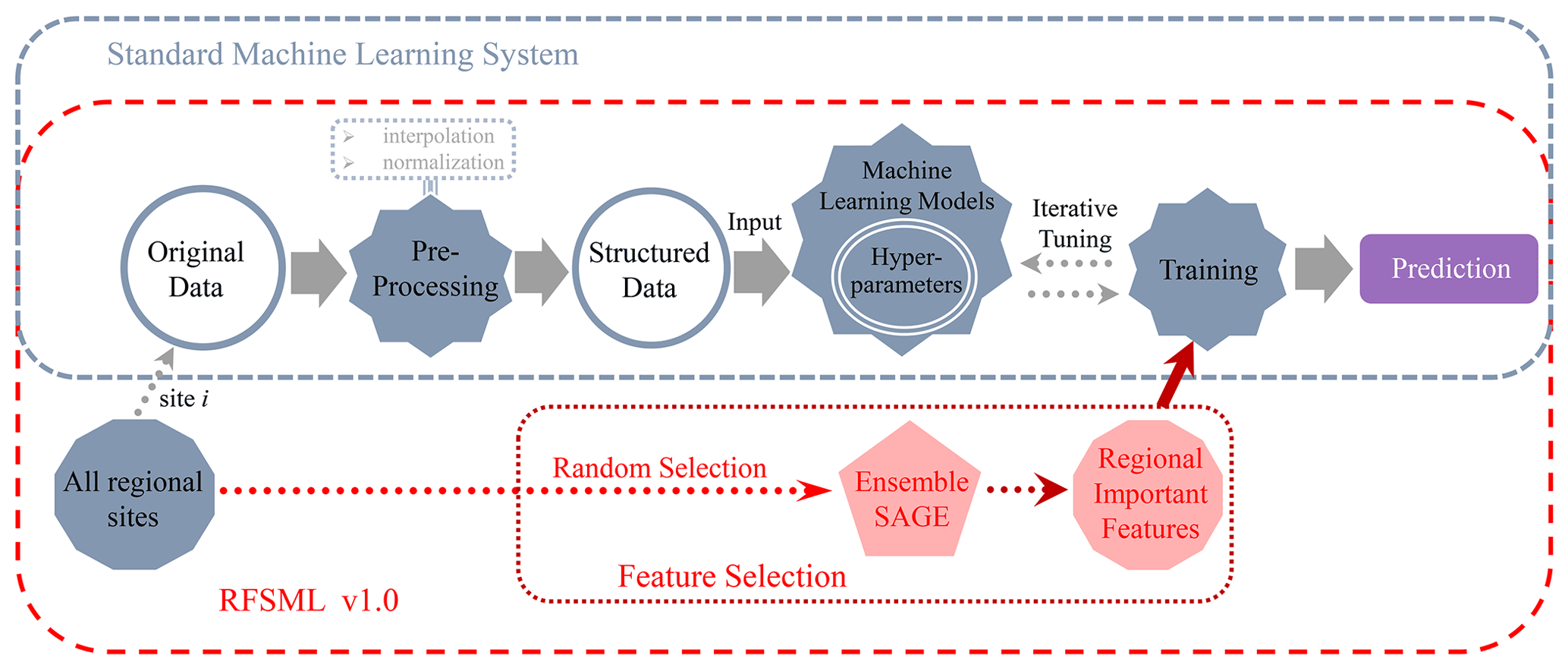
As mentioned before, some features are residual, and the feature subset can provide sufficient predictive power and less noise for ℱ. Thus, the proposed RFSML utilized SAGE to obtain the optimal feature subsets. Considering the computational efficiency, we divided the total national air quality monitoring stations into six types, each of which randomly selected the air quality monitoring stations for feature selection. Given any feature subset , the machine learning models can be described as follows:
2.2.2 Machine learning models
Different machine learning algorithms have been used to forecast PM2.5 because they can provide promising approaches to handle complex nonlinear relationships. Each algorithm exhibits advantages and drawbacks. Of the machine learning models, typical boosting (e.g., GB) and bagging (e.g., RF) algorithms are widely applied in regression analysis using a set of decision trees. Additionally, artificial neural network models (e.g., MLP) that are composed of many processing elements can successfully perform nonlinear mapping. Thus, to evaluate the robustness of the feature selection, all of the prediction algorithms mentioned above were tested in the present study.
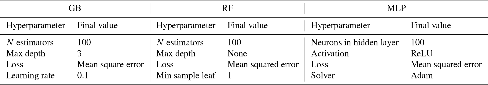
The original data in Fig. 3 were converted into a 27-dimensional matrix (n=27) after preprocessing. On the basis of the auto-correlation and partial auto-correlation results, a time step tp=9 h was selected for the forecast. The prediction horizon h spans from 1 to 24 h. Then, the matrix was converted into supervised learning based on tp and h. The model hyperparameters (Table 4) were designed for each predicting algorithm using 10-fold cross-validation and then fit to each predicting algorithm. Note that “none” for the max depth of RF means “nodes are expanded until all leaves are pure or until all leaves contain less than min_samples_split samples” in Scikit learn (Pedregosa et al., 2011).
2.2.3 SAGE-based regional feature selection
Many methods have been utilized to investigate the significance of features for machine learning models. The game-theoretic method based on the Shapley value is the most widely adopted. Unlike SHAP, a well-known method for explaining individual predictions, SAGE explains model behavior across the entire dataset. Global model interpretability helps us understand the distribution of target outcomes based on the features (Molnar, 2020), which is useful for finding the typical features of each region. There are two outstanding added values of SAGE (Covert et al., 2020). The first is its ability to remove large subsets of features because only removing individual features gives too little significance to features with sufficient proxies, such as in permutation tests. The other advantage of SAGE is its ability to select notable features from their conditional distribution instead of their marginal distribution, reducing unlikely feature combinations.
Given the function Wℱ, which represents the predictive power of a machine learning model ℱ with subsets of features xs⊆xn, the SAGE algorithm can be written as follows:
where ℓ means the loss function that measures the root mean squared error (RMSE) or mean absolute error (MAE); is the prediction from ℱ; y represents the target variable; sets S and N store and , respectively; i is each single variable where i∈N; and n is the length of N. Wℱ increases with a decline in the loss function for any subset S⊆N (note the minus sign in front of the loss function in Eq. 3). Equation (4) represents the Shapley value that is the weighted average of the incremental changes from adding i to subsets (Covert et al., 2020). The more a feature contributes to the prediction from ℱ, the larger the positive values ϕi(Wℱ) would become.
The computational costs of the SAGE analysis over machine learning models including RF, GB, and MLP are presented in Sect. 3.1. They are much more expensive than the model training and therefore cannot be repeated over all sites. Meanwhile, air pollution in nearby monitoring stations has inherent similarities because its forcing factors, i.e., meteorological and emission variables, are closely related in a given region. As in Zhai et al. (2019), all the available sites were partitioned into six categories in the present study: the North China Plain (NCP; 34–41∘ N, 113–119∘ E), Yangtze River Delta (YRD; 30–33∘ N, 119–122∘ E), Pearl River Delta (PRD; 21.5–24∘ N, 112–115.5∘ E), Sichuan Basin (SCB; 28.5–31.5∘ N, 103.5–107∘ E) Fenwei Plain (FWP; 33–35∘ N, 106.25–111.25∘ E; 35–37∘ N, 108.75–113.75∘ E), and the remainder of China. The locations of these regions can be found in Fig. 1. Therefore, we propose the regional future selection in which SAGE is only implemented in limited ensemble sites that are randomly selected in a given region, and the selected features would be used for model training and prediction at each regional site.
The framework of regional feature selection, as illustrated by Algorithm 1, is as follows. A total of 15 ensemble stations are randomly selected in each of the six regions. Taking NCP as an example, the significance of the features of the ensemble monitoring stations with four prediction horizons (6, 12, 18, and 24 h) and three prediction algorithms is analyzed using SAGE algorithms. Then, the outcomes of the ensemble-SAGE model are ranked, as displayed in the heatmap in Fig. 4. The heatmap highlights the significant features. PM2.5, CO, and v10 typically exhibit higher ranks in the 15 random monitoring stations and four prediction horizons. The heatmaps of the ensemble-SAGE analyses of the other five regions can be found in Figs. S2–S18 in the Supplement. The feature significance in different regions is ranked by the sum of the SAGE values in the ensemble monitoring stations and four prediction horizons, as displayed in Fig. 5. The feature selection based on the ensemble-SAGE analysis concerning Fig. 5 is explained in Sect. 3.2. Note that we also tried random ensemble numbers 10 and 20 in NCP key feature extraction using the MLP model at several prediction horizons. The choice of 15 is shown to give the most robust result with a minimum computation cost, and it is therefore used for all regional feature selections in this study.
Algorithm 1Regional feature selection.
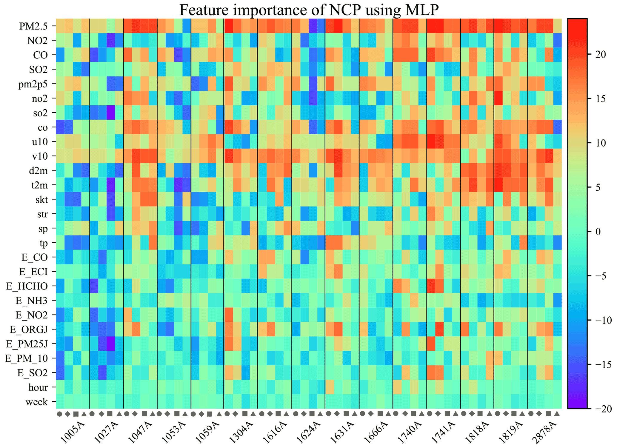
Figure 4Heatmap of all empirical features with 15 random monitoring stations in NCP and four prediction horizons. The circle, diamond, square, and triangle represent the 6, 12, 18, and 24 h prediction horizons, respectively. The heatmap is based on the SAGE analysis ranking of features training by MLP. The warmer the row color, the more significant the corresponding feature.
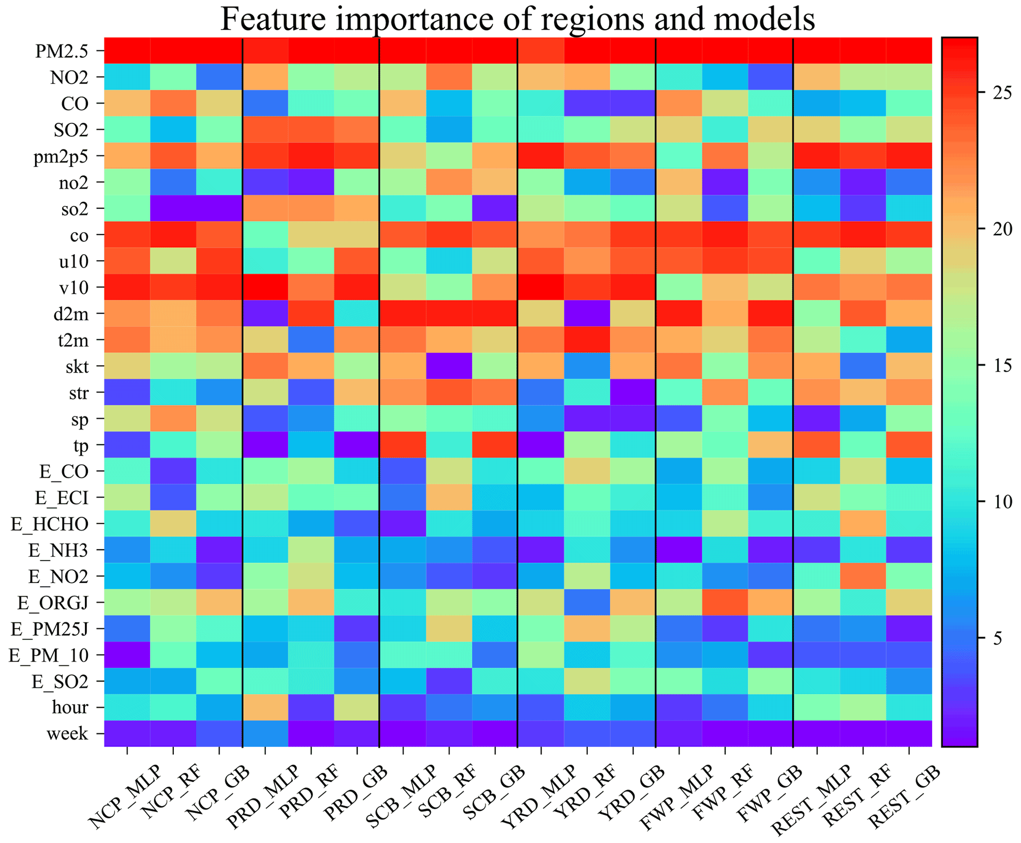
Figure 5Heatmap of empirical features for six regions with three machine learning models. Each column represents the rearrangement of the sum of 15 monitoring stations and four prediction horizons. Black vertical lines are used to distinguish each region. The warmer the row color, the more critical the corresponding feature.
3.1 Computational complexity analysis
Instead of performing feature selection for every forecast model independently, our proposed ensemble-SAGE analysis successfully interprets the important regional features for PM2.5 prediction with substantially less computation complexity. In addition, the regional feature selection improves the forecast accuracy and saves significant computing power for the machine learning model training by excluding redundant inputs and speeding up the model convergence. In this study, all computations concerning the SAGE-based feature selection and machine learning model training were conducted on several nodes configured with 4×16-core 2.1 GHz Intel Xeon E5-2620 v4 CPUs and with 64 GB of memory.
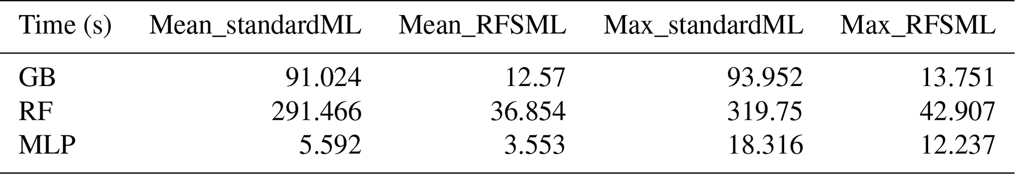
The computational cost of SAGE varies significantly, with average times of 7353, 3891, and 3325 s when using GB, RF, and MLP, respectively. The maximum time costs reach 61 209, 65 127, and 23 931 s with GB, RF, and MLP, respectively. Thus, using SAGE for each PM2.5 forecasting model with different air quality monitoring stations, prediction horizons, and machine learning models is time-consuming. As illustrated in Table 5, the time cost for the three machine learning model training sessions is greatly reduced using the inputs from SAGE-based regional feature selection.
Table 5Summary of mean and maximum time costs of machine learning model training.
3.2 Regional feature selection analysis
The results of the SAGE-based regional feature selection concerning the three machine learning models, six partitioned regions, and four forecasting horizons are discussed in this section. Taking the NCP as an example, critical features that govern the performance of PM2.5 forecasting vary across stations and prediction horizons, as illustrated in Fig. 4. However, PM2.5, CO, and v10 (features) play an overwhelmingly positive role in MLP-based PM2.5 forecasting for most selected stations and predicting horizons. This result indicates that these three features suit all of the stations in the NCP. SAGE analysis heatmaps for other regions or using different prediction algorithms can be found in Figs. S2–S18. Consistently critical features can be easily extracted from the five megacity cluster regions using our selection method. However, they are difficult to extract from the remaining area of China. This area does not have universal key features because its stations are spread widely across China and therefore exhibit substantially different air quality patterns. An improved station clustering method can help solve this issue and will be explored in our future research.
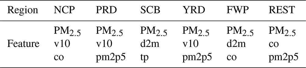
To extract the important robust features that fit all stations in a given region, we summed and ranked the SAGE analysis values in the ensemble monitoring stations and prediction horizons. The ensemble-SAGE ranking is displayed in Fig. 5. There are consistent, crucial features in the six cluster regions, regardless of the prediction algorithm or horizon. PM2.5 is the most critical feature for predicting its trend at a particular region and with a particular prediction algorithm. In addition to PM2.5, two variables from CAMS reanalysis, co and pm2p5, are critical across all regions. This result suggests that the forecast of these variables from CAMS reanalysis can help capture the varying trend in the machine learning models, even though the predictions are different from the actual values. By contrast, time factors (week and hour information) are the least important features for short-term prediction. This result is consistent with that of Hu et al. (2014), where no distinct weekday/weekend difference was observed for PM2.5 in the NCP and PRD. Considering their generality and robustness, we selected the top three critical features for each region, as illustrated in Table 6. Note that the ensemble SAGE analysis selected different key features in different regions. In the NCP, the simulation of CO from CAMS reanalysis, which is a representative air pollutant, includes valuable information other than CO observations. This result implies that local precursor emissions are a major contributor to PM pollution (Guo et al., 2016), and non-point source pollution may be more favorable for PM2.5 forecasting. Additionally, v10, which represents regional transmission, is a critical feature for PM2.5 forecasting in the NCP, PRD, and YRD. This result indicates that regional transmission plays a vital role in these three regions (Chen et al., 2017; Liu et al., 2017). This finding is consistent with findings reported in recent studies. Zhang et al. (2018) found that the anomalously high, normalized, and near-surface meridional wind is typically the primary cause of the severe haze in the NCP using a chemical transport model. Huang et al. (2018) illustrated that regional transport accounts for over half of PM2.5 under the polluted northerly airflow in winter. T. Ma et al. (2019) discovered that the regional PM2.5 pollution in winter is primarily from northern and eastern China using a trajectory model. However, v10 is less significant in the SCB. This result is because of the blocking effect of the plateau terrain on the northeasterly winds (Shu et al., 2021); hence, winds are frequently static, particularly in winter and autumn (Liao et al., 2017). By contrast, d2m and tp are crucial features for hourly PM2.5 forecasting in the SCB. This finding may be because polluted weather patterns are typically associated with higher relative humidity in that area, and tp, representing rainfall, is vital to eliminate air pollution in a basin (Zhan et al., 2019).
3.3 Performance of RFSML
This section presents the forecasting skill of the proposed RFSML system driven by regional features selected by the ensemble-SAGE-based model. The results are also compared with those of a standard machine learning forecasting model and fourth-generation ECMWF global reanalysis data. The latter is referred to as the benchmark of chemical transport models. To highlight the improvements by using the selected key features, the regional performance which represents the average of the forecasting performance in all sites of the given region is introduced.
Figure 6 displays the times series of the simulated PM2.5 for the three forecasting systems (MLP model and at a predicting horizon of 12 h) versus observational data. Each subplot represents a random monitoring station in the corresponding five megacity cluster regions. The subplots illustrate the typical behaviors observed for the other monitoring stations, machine learning models, and prediction horizons. Both the standard machine learning and RFSML models outperform the simple CTM. This result indicates that the machine learning algorithms are superior in air pollution prediction (Pérez et al., 2000). Additionally, PM2.5 predictions with selected key features perform better than the standard machine learning forecast that uses all related features. The GB and RF machine learning models used in this study also show steady improvements.
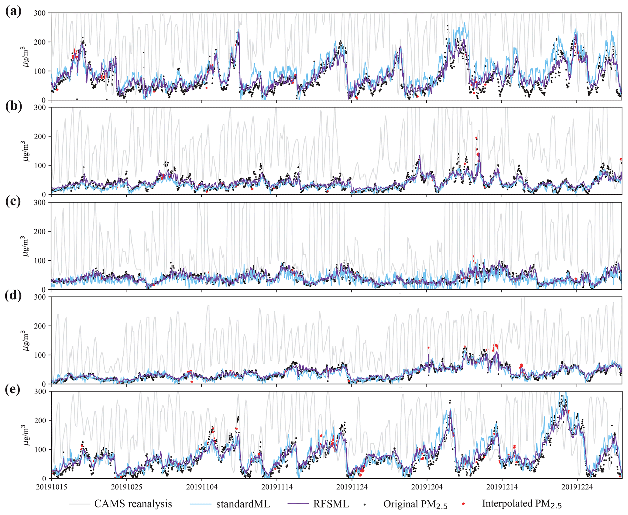
Figure 6Time series of test time in five megacity cluster regions. The black dots and red pentacles represent original and interpolated PM2.5 respectively. The solid lines in light gray, light blue, and dark violet represent prediction of CAMS reanalysis, the standard machine learning system and RFSML respectively. Panels (a)–(e) represent a random site in NCP, YRD, PRD, SCB, and FWP respectively. Note that those are predictions 12 h in advance, which are in parallel with CAMS reanalysis's predicting horizon, and the machine learning model used here is MLP.
Both the RFSML and standard machine learning predictions typically underestimate high PM2.5 concentrations as the prediction horizon increases. This underestimation can be ascribed to three primary possible reasons. First, the correct features are difficult to obtain, and unsuitable features can bring significant bias and noise into the prediction algorithms. Second, the construction of our prediction algorithm network may be insufficiently complex or deep to determine the actual relationship between features and the PM2.5. However, considering the purpose of a real-time forecast, the time to forecast, which is closely related to the complexity of the prediction algorithm network, cannot be too long. Third, considering our test period only included late autumn and early winter of 2019, the training and validation periods only included autumn and winter of 2018, which is too short for a prediction algorithm to learn the complex relationship for hourly PM2.5 forecasting. Seasonal training and validation may obtain satisfactory outcomes for a particular seasonal forecast (Bai et al., 2019).
Figure 7 displays the spatial distribution of the RMSEs (columns a and b) and MAEs (columns c and d) of the PM2.5 forecast for all stations either using the standard machine learning or RFSML system at a forecasting horizon of 12 h. The RMSEs and MAEs significantly decreased when using the selected key features for all three machine learning models, particularly in regions with severe PM2.5 pollution, e.g., the NCP and FWP. This consistent improvement also occurs when the forecast horizon changes to 6, 18, and 24 h, and the results are illustrated in Figs. S19–S21 in the Supplement.
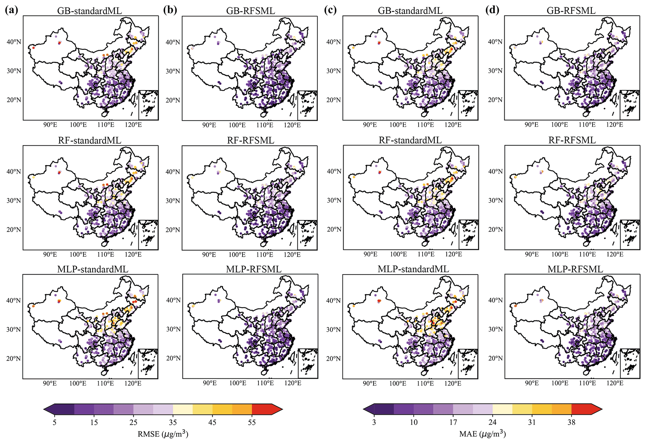
Figure 7Spatial distribution of RMSEs and MAEs at a prediction horizon of 12 h. Panels (a) and (c) are results of standard machine learning system, while panels (b) and (d) are results of RFSML. The cooler the color tone, the lower the RMSEs and MAEs and thus the better the prediction performance.
A modified Taylor diagram (Taylor, 2005) is plotted in Fig. 8 to show the overall outcome. RFSML forecasts with selected features typically exhibit a lower RMSE and higher R than the standard forecasts. The best improvement is obtained when the deep learning (MLP) model is used, while forecasts with the selected new features in the RF model are not significantly improved and even not as good as with forecasts that use all features.
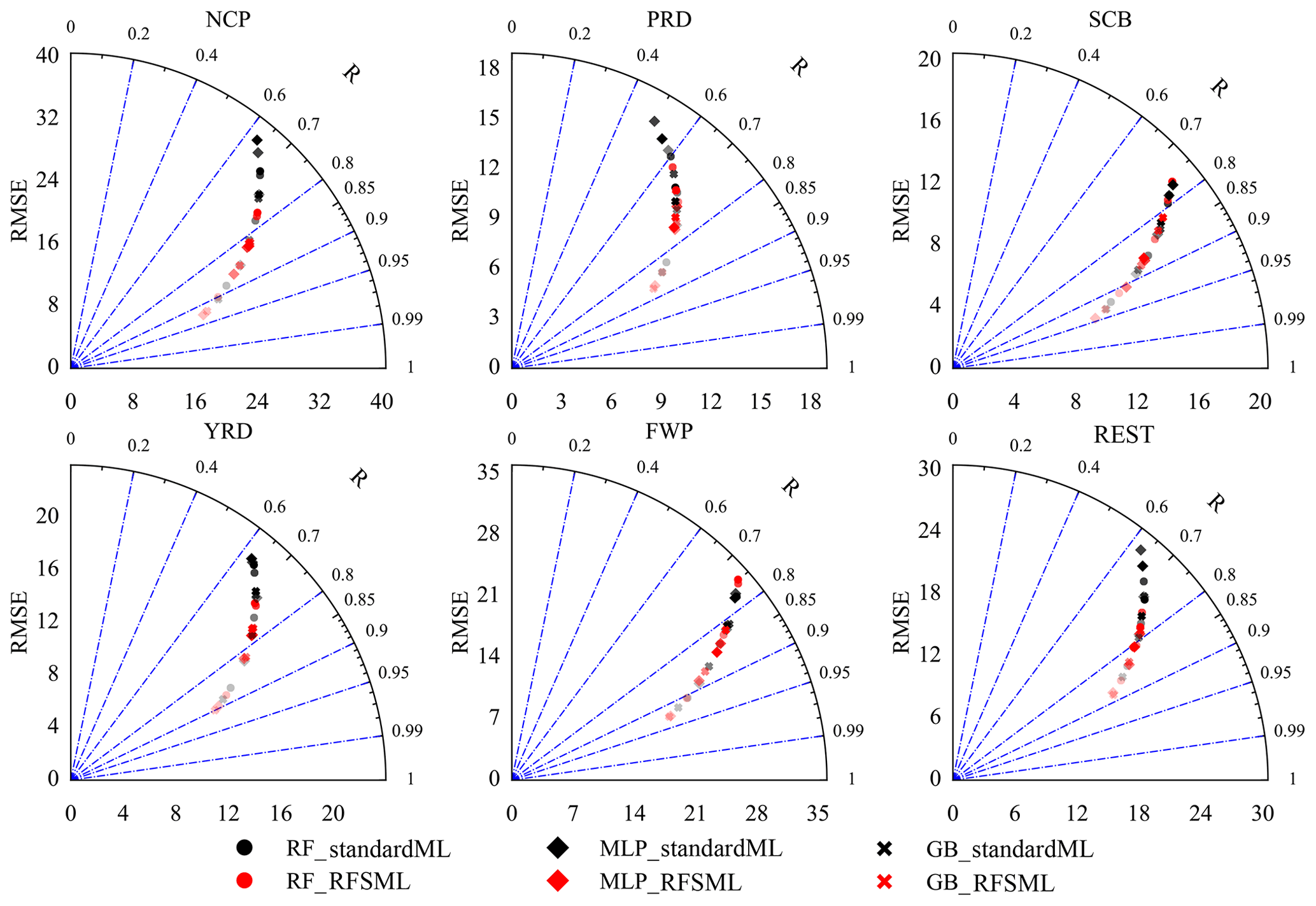
Figure 8A modified Taylor diagram that illustrates RMSE and correlation coefficient values in six regions. The black and red colors represent forecasts with standard machine learning models and RFSML. Round, diamond, and fork shapes represent RF, MLP, and GB respectively. The transparency of markers indicates the four prediction horizons, where the transparency increases as the forecast hours increase.
This result can be explained by the characteristics of the two types of prediction algorithms. RF increases the diversity of the trees through the bootstrapped aggregation of several regression trees (bagging) (Brokamp et al., 2017). It has the advantage of maintaining low bias because tree-based methods with bagging can reduce the variance of an estimated prediction function. Some uninformative features can be ignored through bagging; i.e., RF reduces the high variance by growing the individual trees to a deep level and then making their predictions, typically through averaging (Liaw and Wiener, 2002). By contrast, MLP, which implements the global approximation strategy (Osowski et al., 2004), may face problems of multicollinearity and noise caused by uninformative features.
The RMSE increases and R declines with an increase in the prediction horizons across all regions and machine learning models in general. The average coefficient of determination (R2) of the 24 h forecast (the maximum horizon set in this study) based on the three machine learning models increases from 0.47 to 0.65 in the NCP, from 0.41 to 0.52 in the PRD, from 0.62 to 0.67 in the SCB, from 0.44 to 0.57 in the YRD, and from 0.62 to 0.65 in the FWP when using the ensemble-SAGE analysis-based feature selection. This results indicate that the RFSML system can provide the operational PM2.5 forecast with a maximum horizon of 24 h.
To further confirm the predictive capability in a rolling way, we make forecasts over a less polluted month, April 2020. Specific results can be found in Table S1 in the Supplement. Steady improvement of predicting performance is still achieved by RFSML. Time series, as given in Fig. S22 in the Supplement, show similar results as the main text that RFSML has better predictive ability than standard machine learning. As is illustrated in Figs. S23–S24 in the Supplement, RFSML has both lower RMSE and MAE values than standard machine learning, which implies the advantage of RFSML.
Machine learning models have been successfully utilized in air quality forecasts worldwide because of their high computational efficiency and accuracy. However, substantial room for improvement remains. In this study, we developed the RFSML v1.0 system, which can predict national air quality with high accuracy in real time in China.
In a standard machine learning system, all related features are typically utilized in model training and prediction. However, the high dimensionality and redundant input data may lead to increased complexity and machine learning model over-fitting. To overcome this obstacle, we combined an ensemble-SAGE analysis with our RFSML system. This method extracts the key features in a given region at an affordable extra cost, and the significance of these regional selected features are explained physically. Compared with the standard machine learning system that was fed with all relative features, the RFSML system driven by the selected key features resulted in superior interpretability, less training time, and more accurate predictions. Statistically, the average RMSE and MAE of predictions were reduced from 24.74 and 16.54 µg m−3 to 21.54 and 13.7 µg m−3, respectively, with RFSML. Additionally, R2 increased from 0.6 to 0.7, and the average forecasting model training cost was reduced from 129.36 to 17.66 s. Among the three machine learning models studied, the prediction performance of RFSML with MLP exhibited the greatest increase, with R2 increasing from 0.55 to 0.72. By contrast, RF exhibited the least improvement, with R2 increasing from 0.61 to 0.66. In addition, RF and GB were more robust than MLP for certain underlying uninformative features, while MLP was more susceptible to over-fitting. Meanwhile, RFSML provides only predictions over the air quality monitoring sites where historical data are available for machine learning model training, instead of a gridded forecast. A Bayesian-theory-based prediction fusion is being explored now to extend the RFSML forecast available at single stations to a gridded one.
The six-region partition used here was empirical and not based on science. Additionally, stations in a given region may exhibit different air quality patterns, particularly in the “remainder” region. Therefore, our ensemble-SAGE analysis does not always select the representative feature, limiting the machine model interpretability and prediction ability. A more scientific station partition like spatial clustering would be determined for future studies.
Based on the results of this study, the RFSML system can accurately predict air quality in the short term at the national scale; this renders it valuable for health professionals and policy makers in terms of providing early warning to population categories more susceptible to air pollution (e.g., children, elderly, and people with respiratory or cardiovascular issues) and reducing and regulating air pollution.
The ground-based air quality monitoring observations are from the network established by the China Ministry of Environmental Protection and accessible via https://quotsoft.net/air/ (last access: June 2022). The measurements used in this study also are archived on Zenodo (https://doi.org/10.5281/zenodo.6551820, Fang, 2022). The RFSML algorithm is in the Python environment and is archived on Zenodo (https://doi.org/10.5281/zenodo.6551850, , Fang, 2022).
The supplement related to this article is available online at: https://doi.org/10.5194/gmd-15-7791-2022-supplement.
JJ conceived the study and designed the RFSML system. LF wrote the code of RFSML and carried out the prediction and evaluation. HXL, AS, CX, TD, and HL provided useful comments on the paper. LF prepared the manuscript with contributions from JJ and all other co-authors.
The contact author has declared that none of the authors has any competing interests.
Publisher's note: Copernicus Publications remains neutral with regard to jurisdictional claims in published maps and institutional affiliations.
This work is supported by the National Natural Science Foundation of China (grant nos. 42105109 and 42021004) and the Natural Science Foundation of Jiangsu Province (grant nos. BK20210664 and BK20220031).
This paper was edited by Augustin Colette and reviewed by two anonymous referees.
Abu Awad, Y., Koutrakis, P., Coull, B. A., and Schwartz, J.: A spatio-temporal prediction model based on support vector machine regression: Ambient Black Carbon in three New England States, Environ. Res., 159, 427–434, https://doi.org/10.1016/j.envres.2017.08.039, 2017. a
Altmann, A., Toloşi, L., Sander, O., and Lengauer, T.: Permutation importance: a corrected feature importance measure, Bioinformatics, 26, 1340–1347, https://doi.org/10.1093/bioinformatics/btq134, 2010. a
Bai, Y., Li, Y., Zeng, B., Li, C., and Zhang, J.: Hourly PM2.5 concentration forecast using stacked autoencoder model with emphasis on seasonality, J. Clean. Prod., 224, 739–750, 2019. a
Bartier, P. M. and Keller, C.: Multivariate interpolation to incorporate thematic surface data using inverse distance weighting (IDW), Comput. Geosci., 22, 795–799, https://doi.org/10.1016/0098-3004(96)00021-0, 1996. a
Bey, I., Jacob, D. J., Yantosca, R. M., Logan, J. A., Field, B. D., Fiore, A. M., Li, Q., Liu, H. Y., Mickley, L. J., and Schultz, M. G.: Global modeling of tropospheric chemistry with assimilated meteorology: Model description and evaluation, J. Geophys. Res.-Atmos., 106, 23073–23095, https://doi.org/10.1029/2001JD000807, 2001. a
Brokamp, C., Jandarov, R., Rao, M., LeMasters, G., and Ryan, P.: Exposure assessment models for elemental components of particulate matter in an urban environment: A comparison of regression and random forest approaches, Atmos. Environ., 151, 1–11, https://doi.org/10.1016/j.atmosenv.2016.11.066, 2017. a
Burnett, R., Chen, H., Szyszkowicz, M., Fann, N., Hubbell, B., Pope, C. A., Apte, J. S., Brauer, M., Cohen, A., Weichenthal, S., Coggins, J., Di, Q,. Brunekreef, B., Frostad, J., Lim, S. S., Kan, H., Walker, K. D., Thurston, G. D., Hayes, R. B., Lim, C. C., Turner, M. C., Jerrett, M., Krewski, D., Gapstur, S. M., Diver, W. R., Ostro, B., Goldberg, D., Crouse, D. L., Martin, R. V., Peters, P., Pinault, L., Tjepkema, M., van, Donkelaar. A., Villeneuve, P. J., Miller, A. B., Yin, P., Zhou, M., Wang, L., Janssen, NAH., Marra, M., Atkinson, R. W., Tsang, H., Quoc, Thach. T., Cannon, J. B., Allen, R. T., Hart, J. E., Laden, F., Cesaroni, G., Forastiere, F., Weinmayr, G., Jaensch, A., Nagel, G., Concin, H., and Spadaro, J. V.: Global estimates of mortality associated with long-term exposure to outdoor fine particulate matter, P. Natl. Acad. Sci. USA, 115, 9592–9597, 2018. a
Cao, D., Chen, Y., Chen, J., Zhang, H., and Yuan, Z.: An improved algorithm for the maximal information coefficient and its application, Roy. Soc. Open Sci., 8, 201424, https://doi.org/10.1098/rsos.201424, 2021. a
Casalicchio, G., Molnar, C., and Bischl, B.: Visualizing the Feature Importance for Black Box Models, in: Machine Learning and Knowledge Discovery in Databases, edited by: Berlingerio, M., Bonchi, F., Gärtner, T., Hurley, N., and Ifrim, G., Springer International Publishing, Cham, 655–670, https://doi.org/10.1007/978-3-030-10925-7_40, 2019. a
Chandrashekar, G. and Sahin, F.: A survey on feature selection methods, Comput. Electr. Eng., 40, 16–28, https://doi.org/10.1016/j.compeleceng.2013.11.024, 2014. a
Chen, D., Liu, X., Lang, J., Zhou, Y., Wei, L., Wang, X., and Guo, X.: Estimating the contribution of regional transport to PM2.5 air pollution in a rural area on the North China Plain, Sci. Total Environ., 583, 280–291, https://doi.org/10.1016/j.scitotenv.2017.01.066, 2017. a
Chen, Y., Zeng, Y., Luo, F., and Yuan, Z.: A new algorithm to optimize maximal information coefficient, PloS one, 11, e0157567, https://doi.org/10.1371/journal.pone.0157567, 2016. a
Cobourn, W. G.: An enhanced PM2.5 air quality forecast model based on nonlinear regression and back-trajectory concentrations, Atmos. Environ., 44, 3015–3023, https://doi.org/10.1016/j.atmosenv.2010.05.009, 2010. a
Copernicus Climate Change Service (C3S): ERA5: Fifth generation of ECMWF atmospheric reanalyses of the global climate. Copernicus Climate Change Service Climate Data Store (CDS), https://cds.climate.copernicus.eu/cdsapp#!/home (last access: June 2022), 2017. a
Covert, I., Lundberg, S. M., and Lee, S.-I.: Understanding Global Feature Contributions With Additive Importance Measures, in: Advances in Neural Information Processing Systems, vol. 33, edited by: Larochelle, H., Ranzato, M., Hadsell, R., Balcan, M. F., and Lin, H., Curran Associates, Inc., 17212–17223, https://proceedings.neurips.cc/paper/2020/file/c7bf0b7c1a86d5eb3be2c722cf2cf746-Paper.pdf (last access: June 2022), 2020. a, b, c, d
Di, Q., Amini, H., Shi, L., Kloog, I., Silvern, R., Kelly, J., Sabath, M. B., Choirat, C., Koutrakis, P., Lyapustin, A., Wang, Y., Mickley, L. J., and Schwartz, J.: An ensemble-based model of PM2.5 concentration across the contiguous United States with high spatiotemporal resolution, Environ. Int., 130, 104909, https://doi.org/10.1016/j.envint.2019.104909, 2019. a
Fan, T., Liu, X., Ma, P.-L., Zhang, Q., Li, Z., Jiang, Y., Zhang, F., Zhao, C., Yang, X., Wu, F., and Wang, Y.: Emission or atmospheric processes? An attempt to attribute the source of large bias of aerosols in eastern China simulated by global climate models, Atmos. Chem. Phys., 18, 1395–1417, https://doi.org/10.5194/acp-18-1395-2018, 2018. a
Fang, L.: The ground observations for RFSML, Zenodo [data set and code], https://doi.org/10.5281/zenodo.6551820, 2022. a, b
Fernando, H., Mammarella, M., Grandoni, G., Fedele, P., Di Marco, R., Dimitrova, R., and Hyde, P.: Forecasting PM10 in metropolitan areas: Efficacy of neural networks, Environ. Pollut., 163, 62–67, https://doi.org/10.1016/j.envpol.2011.12.018, 2012. a
Fritsch, F. N. and Carlson, R. E.: Monotone piecewise cubic interpolation, SIAM J. Numer. Anal., 17, 238–246, 1980. a
Fryer, D. V., Strümke, I., and Nguyen, H.: Shapley values for feature selection: The good, the bad, and the axioms, arXiv [preprint], https://doi.org/10.48550/arXiv.2102.10936, 22 February 2021. a
Golizadeh Akhlaghi, Y., Aslansefat, K., Zhao, X., Sadati, S., Badiei, A., Xiao, X., Shittu, S., Fan, Y., and Ma, X.: Hourly performance forecast of a dew point cooler using explainable Artificial Intelligence and evolutionary optimisations by 2050, Appl. Energ., 281, 116062, https://doi.org/10.1016/j.apenergy.2020.116062, 2021. a
Grell, G. A., Peckham, S. E., Schmitz, R., McKeen, S. A., Frost, G., Skamarock, W. C., and Eder, B.: Fully coupled “online” chemistry within the WRF model, Atmos. Environ., 39, 6957–6975, https://doi.org/10.1016/j.atmosenv.2005.04.027, 2005. a
Guo, J., He, J., Liu, H., Miao, Y., Liu, H., and Zhai, P.: Impact of various emission control schemes on air quality using WRF-Chem during APEC China 2014, Atmos. Environ., 140, 311–319, https://doi.org/10.1016/j.atmosenv.2016.05.046, 2016. a
Guyon, I. and Elisseeff, A.: An introduction to variable and feature selection, J. Mach. Learn. Res., 3, 1157–1182, 2003. a
Hao, X., Li, J., Wang, H., Liao, H., Yin, Z., Hu, J., Wei, Y., and Dang, R.: Long-term health impact of PM2.5 under whole-year COVID-19 lockdown in China, Environ. Pollut., 290, 118118, https://doi.org/10.1016/j.envpol.2021.118118, 2021. a
Hu, J., Wang, Y., Ying, Q., and Zhang, H.: Spatial and temporal variability of PM2.5 and PM10 over the North China Plain and the Yangtze River Delta, China, Atmos. Environ., 95, 598–609, https://doi.org/10.1016/j.atmosenv.2014.07.019, 2014. a
Hu, J., Li, X., Huang, L., Ying, Q., Zhang, Q., Zhao, B., Wang, S., and Zhang, H.: Ensemble prediction of air quality using the WRF/CMAQ model system for health effect studies in China, Atmos. Chem. Phys., 17, 13103–13118, https://doi.org/10.5194/acp-17-13103-2017, 2017. a
Huang, L., Liu, S., Yang, Z., Xing, J., Zhang, J., Bian, J., Li, S., Sahu, S. K., Wang, S., and Liu, T.-Y.: Exploring deep learning for air pollutant emission estimation, Geosci. Model Dev., 14, 4641–4654, https://doi.org/10.5194/gmd-14-4641-2021, 2021. a
Huang, X.-F., Zou, B.-B., He, L.-Y., Hu, M., Prévôt, A. S. H., and Zhang, Y.-H.: Exploration of PM2.5 sources on the regional scale in the Pearl River Delta based on ME-2 modeling, Atmos. Chem. Phys., 18, 11563–11580, https://doi.org/10.5194/acp-18-11563-2018, 2018. a
Hutzell, W. T. and Luecken, D. J.: Fate and transport of emissions for several trace metals over the United States, Sci. Total Environ., 396, 164–179, https://doi.org/10.1016/j.scitotenv.2008.02.020, 2008. a
Inness, A., Ades, M., Agustí-Panareda, A., Barré, J., Benedictow, A., Blechschmidt, A.-M., Dominguez, J. J., Engelen, R., Eskes, H., Flemming, J., Huijnen, V., Jones, L., Kipling, Z., Massart, S., Parrington, M., Peuch, V.-H., Razinger, M., Remy, S., Schulz, M., and Suttie, M.: The CAMS reanalysis of atmospheric composition, Atmos. Chem. Phys., 19, 3515–3556, https://doi.org/10.5194/acp-19-3515-2019, 2019. a, b
Jeong, J. I. and Park, R. J.: Efficacy of dust aerosol forecasts for East Asia using the adjoint of GEOS-Chem with ground-based observations, Environ. Pollut., 234, 885–893, https://doi.org/10.1016/j.envpol.2017.12.025, 2018. a
Jin, J., Lin, H. X., Segers, A., Xie, Y., and Heemink, A.: Machine learning for observation bias correction with application to dust storm data assimilation, Atmos. Chem. Phys., 19, 10009–10026, https://doi.org/10.5194/acp-19-10009-2019, 2019. a
Jothi, N., Husain, W., and Rashid, N. A.: Predicting generalized anxiety disorder among women using Shapley value, J. Infect. Public Heal., 14, 103–108, https://doi.org/10.1016/j.jiph.2020.02.042, 2021. a
Ke, H., Gong, S., He, J., Zhang, L., Cui, B., Wang, Y., Mo, J., Zhou, Y., and Zhang, H.: Development and application of an automated air quality forecasting system based on machine learning, Sci. Total Environ., 806, 151204, https://doi.org/10.1016/j.scitotenv.2021.151204, 2021. a
Kincaid, D., Kincaid, D. R., and Cheney, E. W.: Numerical analysis: mathematics of scientific computing, vol. 2, American Mathematical Soc., ISBN 978-0-8218-4788-6, 2009. a
Kinney, J. B. and Atwal, G. S.: Equitability, mutual information, and the maximal information coefficient, P. Natl. Acad. Sci. USA, 111, 3354–3359, 2014. a
Leufen, L. H., Kleinert, F., and Schultz, M. G.: MLAir (v1.0) – a tool to enable fast and flexible machine learning on air data time series, Geosci. Model Dev., 14, 1553–1574, https://doi.org/10.5194/gmd-14-1553-2021, 2021. a
Li, M., Liu, H., Geng, G., Hong, C., Liu, F., Song, Y., Tong, D., Zheng, B., Cui, H., Man, H., Zhang, Q., and He, K.: Anthropogenic emission inventories in China: a review, Natl. Sci. Rev., 4, 834–866, https://doi.org/10.1093/nsr/nwx150, 2017. a, b
Li, X., Peng, L., Yao, X., Cui, S., Hu, Y., You, C., and Chi, T.: Long short-term memory neural network for air pollutant concentration predictions: Method development and evaluation, Environ. Pollut., 231, 997–1004, https://doi.org/10.1016/j.envpol.2017.08.114, 2017. a
Li, Z., Ma, Z., van der Kuijp, T. J., Yuan, Z., and Huang, L.: A review of soil heavy metal pollution from mines in China: Pollution and health risk assessment, Sci. Total Environ., 468–469, 843–853, https://doi.org/10.1016/j.scitotenv.2013.08.090, 2014. a
Liao, T., Wang, S., Ai, J., Gui, K., Duan, B., Zhao, Q., Zhang, X., Jiang, W., and Sun, Y.: Heavy pollution episodes, transport pathways and potential sources of PM2.5 during the winter of 2013 in Chengdu (China), Sci. Total Environ., 584–585, 1056–1065, https://doi.org/10.1016/j.scitotenv.2017.01.160, 2017. a
Liaw, A. and Wiener, M.: Classification and regression by randomForest, R news, 2, 18–22, 2002. a
Liu, H., He, J., Guo, J., Miao, Y., Yin, J., Wang, Y., Xu, H., Liu, H., Yan, Y., Li, Y., and Zhai, P.: The blue skies in Beijing during APEC 2014: A quantitative assessment of emission control efficiency and meteorological influence, Atmos. Environ., 167, 235–244, https://doi.org/10.1016/j.atmosenv.2017.08.032, 2017. a
Liu, J. and Diamond, J.: China's environment in a globalizing world, Nature, 435, 1179–1186, https://doi.org/10.1038/4351179a, 2005. a
Liu, T., Lau, A. K. H., Sandbrink, K., and Fung, J. C. H.: Time Series Forecasting of Air Quality Based On Regional Numerical Modeling in Hong Kong, J. Geophys. Res.-Atmos., 123, 4175–4196, https://doi.org/10.1002/2017JD028052, 2018. a
Lundberg, S. M. and Lee, S.-I.: A Unified Approach to Interpreting Model Predictions, http://papers.nips.cc/paper/7062-a-unified-approach-to-interpreting-model-predictions.pdf (last access: June 2022), 2017. a, b
Ma, J., Ding, Y., Gan, V. J. L., Lin, C., and Wan, Z.: Spatiotemporal Prediction of PM2.5 Concentrations at Different Time Granularities Using IDW-BLSTM, IEEE Access, 7, 107897–107907, https://doi.org/10.1109/ACCESS.2019.2932445, 2019. a
Ma, T., Duan, F., He, K., Qin, Y., Tong, D., Geng, G., Liu, X., Li, H., Yang, S., Ye, S., Xu, B., Zhang, Q., and Ma, Y.: Air pollution characteristics and their relationship with emissions and meteorology in the Yangtze River Delta region during 2014–2016, J. Environ. Sci.-China, 83, 8–20, https://doi.org/10.1016/j.jes.2019.02.031, 2019. a
Masih, A.: Machine learning algorithms in air quality modeling, Global Journal of Environmental Science and Management, 5, 515–534, 2019. a
Molnar, C.: Interpretable Machine Learning, Lulu.com, 2020. a
Muñoz Sabater, J.: ERA5-Land hourly data from 1950 to 1980, Copernicus Climate Change Service (C3S) Climate Data Store (CDS)[data set], https://doi.org/10.24381/cds.e2161bac, 2021. a
Muñoz-Sabater, J., Dutra, E., Agustí-Panareda, A., Albergel, C., Arduini, G., Balsamo, G., Boussetta, S., Choulga, M., Harrigan, S., Hersbach, H., Martens, B., Miralles, D. G., Piles, M., Rodríguez-Fernández, N. J., Zsoter, E., Buontempo, C., and Thépaut, J.-N.: ERA5-Land: a state-of-the-art global reanalysis dataset for land applications, Earth Syst. Sci. Data, 13, 4349–4383, https://doi.org/10.5194/essd-13-4349-2021, 2021. a
Murray, C. J., Aravkin, A. Y., Zheng, P., Abbafati, C., Abbas, K. M., Abbasi-Kangevari, M., Abd-Allah, F., Abdelalim, A., Abdollahi, M., Abdollahpour, I., and GBD 2019 Risk Factors Collaborators: Global burden of 87 risk factors in 204 countries and territories, 1990–2019: a systematic analysis for the Global Burden of Disease Study 2019, Lancet, 396, 1223–1249, 2020. a
Osowski, S., Siwek, K., and Markiewicz, T.: MLP and SVM networks-a comparative study, in: Proceedings of the 6th Nordic Signal Processing Symposium, 2004, NORSIG 2004, Espoo, Finland, 11–11 June 2004, 37–40, ISBN 951-22-7065-X IEEE,2004. a
Park, H. and Park, D. Y.: Comparative analysis on predictability of natural ventilation rate based on machine learning algorithms, Build. Environ., 195, 107744, https://doi.org/10.1016/j.buildenv.2021.107744, 2021. a
Pedregosa, F., Varoquaux, G., Gramfort, A., Michel, V., Thirion, B., Grisel, O., Blondel, M., Prettenhofer, P., Weiss, R., Dubourg, V., Vanderplas, J., Passos, A., Cournapeau, D., Brucher, M., Perrot, M., and Duchesnay, E.: Scikit-learn: Machine Learning in Python, J. Mach. Learn. Res., 12, 2825–2830, 2011. a
Pérez, P., Trier, A., and Reyes, J.: Prediction of PM2.5 concentrations several hours in advance using neural networks in Santiago, Chile, Atmos. Environ., 34, 1189–1196, https://doi.org/10.1016/S1352-2310(99)00316-7, 2000. a
Pui, D. Y., Chen, S.-C., and Zuo, Z.: PM2.5 in China: Measurements, sources, visibility and health effects, and mitigation, Particuology, 13, 1–26, https://doi.org/10.1016/j.partic.2013.11.001, 2014. a
Qin, Z., Cen, C., and Guo, X.: Prediction of Air Quality Based on KNN-LSTM, J. Phys. Conf. Ser., 1237, 042030, https://doi.org/10.1088/1742-6596/1237/4/042030, 2019. a
Reichstein, M., Camps-Valls, G., Stevens, B., Jung, M., Denzler, J., Carvalhais, N., and Prabhat: Deep learning and process understanding for data-driven Earth system science, Nature, 566, 195–204, 2019. a, b
Rodriguez-Galiano, V., Chica-Olmo, M., Abarca-Hernandez, F., Atkinson, P., and Jeganathan, C.: Random Forest classification of Mediterranean land cover using multi-seasonal imagery and multi-seasonal texture, Remote Sens. Environ., 121, 93–107, https://doi.org/10.1016/j.rse.2011.12.003, 2012. a
Sawaragi, Y., Soeda, T., Tamura, H., Yoshimura, T., Ohe, S., Chujo, Y., and Ishihara, H.: Statistical prediction of air pollution levels using non-physical models, Automatica, 15, 441–451, https://doi.org/10.1016/0005-1098(79)90018-9, 1979. a
Shapley, L. S.: A Value for N-Person Games, RAND Corporation, Santa Monica, CA, https://doi.org/10.7249/P0295, 1952. a, b
Shishegaran, A., Saeedi, M., Kumar, A., and Ghiasinejad, H.: Prediction of air quality in Tehran by developing the nonlinear ensemble model, J. Clean. Prod., 259, 120825, https://doi.org/10.1016/j.jclepro.2020.120825, 2020. a
Shtein, A., Kloog, I., Schwartz, J., Silibello, C., Michelozzi, P., Gariazzo, C., Viegi, G., Forastiere, F., Karnieli, A., and Just, A.: Estimating Daily PM2.5 and PM10 over Italy Using an Ensemble Model, Environ. Sci. Technol., 54, 120–128, https://doi.org/10.1021/acs.est.9b04279, 2020. a
Shu, Z., Liu, Y., Zhao, T., Xia, J., Wang, C., Cao, L., Wang, H., Zhang, L., Zheng, Y., Shen, L., Luo, L., and Li, Y.: Elevated 3D structures of PM2.5 and impact of complex terrain-forcing circulations on heavy haze pollution over Sichuan Basin, China, Atmos. Chem. Phys., 21, 9253–9268, https://doi.org/10.5194/acp-21-9253-2021, 2021. a
Song, C., He, J., Wu, L., Jin, T., Chen, X., Li, R., Ren, P., Zhang, L., and Mao, H.: Health burden attributable to ambient PM2.5 in China, Environ. Pollut., 223, 575–586, https://doi.org/10.1016/j.envpol.2017.01.060, 2017a. a
Song, C., Wu, L., Xie, Y., He, J., Chen, X., Wang, T., Lin, Y., Jin, T., Wang, A., Liu, Y., Dai, Q., Liu, B., Wang, Y., and Mao, H.: Air pollution in China: Status and spatiotemporal variations, Environ. Pollut., 227, 334–347, https://doi.org/10.1016/j.envpol.2017.04.075, 2017b. a, b
Sun, G., Li, J., Dai, J., Song, Z., and Lang, F.: Feature selection for IoT based on maximal information coefficient, Future Gener. Comp. Sy., 89, 606–616, https://doi.org/10.1016/j.future.2018.05.060, 2018. a
Sun, W. and Li, Z.: Hourly PM2.5 concentration forecasting based on feature extraction and stacking-driven ensemble model for the winter of the Beijing-Tianjin-Hebei area, Atmos. Pollut. Res., 11, 110–121, https://doi.org/10.1016/j.apr.2020.02.022, 2020a. a
Sun, W. and Li, Z.: Hourly PM2.5 concentration forecasting based on mode decomposition-recombination technique and ensemble learning approach in severe haze episodes of China, J. Clean. Prod., 263, 121442, https://doi.org/10.1016/j.jclepro.2020.121442, 2020b. a
Sun, W., Zhang, H., Palazoglu, A., Singh, A., Zhang, W., and Liu, S.: Prediction of 24-hour-average PM2.5 concentrations using a hidden Markov model with different emission distributions in Northern California, Sci. Total Environ., 443, 93–103, https://doi.org/10.1016/j.scitotenv.2012.10.070, 2013. a
Taylor, K. E.: Taylor diagram primer, Work. Pap., 1–4, https://www.atmos.albany.edu/daes/atmclasses/atm401/spring_2016/ppts_pdfs/Taylor_diagram_primer.pdf (last access: October 2022), 2005. a
Wu, X., Wang, Y., He, S., and Wu, Z.: PM2.5 / PM10 ratio prediction based on a long short-term memory neural network in Wuhan, China, Geosci. Model Dev., 13, 1499–1511, https://doi.org/10.5194/gmd-13-1499-2020, 2020. a
Xi, X., Wei, Z., Xiaoguang, R., Yijie, W., Xinxin, B., Wenjun, Y., and Jin, D.: A comprehensive evaluation of air pollution prediction improvement by a machine learning method, in: 2015 IEEE International Conference on Service Operations And Logistics, And Informatics (SOLI), Yasmine Hammamet, Tunisia, 15–17 November 2015, 176–181, https://doi.org/10.1109/SOLI.2015.7367615, 2015. a
Xu, M., Jin, J., Wang, G., Segers, A., Deng, T., and Lin, H. X.: Machine learning based bias correction for numerical chemical transport models, Atmos. Environ., 248, 118022, https://doi.org/10.1016/j.atmosenv.2020.118022, 2021. a, b
Xue, T., Zhu, T., Zheng, Y., Liu, J., Li, X., and Zhang, Q.: Change in the number of PM2.5-attributed deaths in China from 2000 to 2010: Comparison between estimations from census-based epidemiology and pre-established exposure-response functions, Environ. Int., 129, 430–437, https://doi.org/10.1016/j.envint.2019.05.067, 2019. a
Yu, S. and Ma, J.: Deep Learning for Geophysics: Current and Future Trends, Rev. Geophys., 59, e2021RG000742, https://doi.org/10.1029/2021RG000742, 2021. a
Zhai, S., Jacob, D. J., Wang, X., Shen, L., Li, K., Zhang, Y., Gui, K., Zhao, T., and Liao, H.: Fine particulate matter (PM2.5) trends in China, 2013–2018: separating contributions from anthropogenic emissions and meteorology, Atmos. Chem. Phys., 19, 11031–11041, https://doi.org/10.5194/acp-19-11031-2019, 2019. a, b, c, d
Zhan, C., Xie, M., Fang, D., Wang, T., Wu, Z., Lu, H., Li, M., Chen, P., Zhuang, B., Li, S., Zhang, Z., Gao, D., Ren, J., and Zhao, M.: Synoptic weather patterns and their impacts on regional particle pollution in the city cluster of the Sichuan Basin, China, Atmos. Environ., 208, 34–47, https://doi.org/10.1016/j.atmosenv.2019.03.033, 2019. a
Zhang, Q., Ma, Q., Zhao, B., Liu, X., Wang, Y., Jia, B., and Zhang, X.: Winter haze over North China Plain from 2009 to 2016: Influence of emission and meteorology, Environ. Pollut., 242, 1308–1318, https://doi.org/10.1016/j.envpol.2018.08.019, 2018. a
Zhang, Q., Wu, S., Wang, X., Sun, B., and Liu, H.: A PM2.5 concentration prediction model based on multi-task deep learning for intensive air quality monitoring stations, J. Clean. Prod., 275, 122722, https://doi.org/10.1016/j.jclepro.2020.122722, 2020. a
Zhang, S.: Nearest neighbor selection for iteratively kNN imputation, J. Syst. Software, 85, 2541–2552, https://doi.org/10.1016/j.jss.2012.05.073, 2012. a
Zhou, G., Xu, J., Xie, Y., Chang, L., Gao, W., Gu, Y., and Zhou, J.: Numerical air quality forecasting over eastern China: An operational application of WRF-Chem, Atmos. Environ., 153, 94–108, https://doi.org/10.1016/j.atmosenv.2017.01.020, 2017. a
Zimmermann, J. and Poppe, D.: A supplement for the RADM2 chemical mechanism: The photooxidation of isoprene, Atmos. Environ., 30, 1255–1269, https://doi.org/10.1016/1352-2310(95)00417-3, 1996. a
Ziomas, I. C., Melas, D., Zerefos, C. S., Bais, A. F., and Paliatsos, A. G.: Forecasting peak pollutant levels from meteorological variables, Atmos. Environ., 29, 3703–3711, https://doi.org/10.1016/1352-2310(95)00131-H, 1995. a