the Creative Commons Attribution 4.0 License.
the Creative Commons Attribution 4.0 License.
 | 27 Jan 2022
Representation of the autoconversion from cloud to rain using a weighted ensemble approach: a case study using WRF v4.1.3
Jinfang Yin
Xudong Liang
Hong Wang
Haile Xue
Cloud and precipitation processes remain among the largest sources of uncertainties in weather and climate modelling, and considerable attention has been paid to improving the representation of the cloud and precipitation processes in numerical models in the last several decades. In this study, we develop a weighted ensemble (named EN) scheme by employing several widely used autoconversion (ATC) schemes to represent the ATC from cloud water to rainwater. One unique feature of the EN approach is that the ATC rate is a weighted mean value based on the calculations from several ATC schemes within a microphysics scheme with a negligible increase in computation cost. The EN scheme is compared with the several commonly used ATC schemes by performing real case simulations. In terms of accumulated rainfall and extreme hourly rainfall rate, the EN scheme provides better simulations than by using the single Berry–Reinhardt scheme, which was originally used in the Thompson scheme. It is worth emphasizing, in the present study, that we only pay attention to the ATC process from cloud water into rainwater with the purpose of improving the modelling of the extreme rainfall events over southern China. Actually, any (source and sink) term in a cloud microphysics scheme can be treated with the same approach. The ensemble method proposed herein appears to have important implications for developing cloud microphysics schemes in numerical models, especially for the models with variable grid resolution, which would be expected to improve the representation of cloud microphysical processes in the weather and climate models.
- Article
(8702 KB) - Full-text XML
- BibTeX
- EndNote


Cloud and precipitation processes and associated feedbacks have been confirmed to cause the largest uncertainties in weather and climate modelling by the Intergovernmental Panel on Climate Change (IPCC) (Houghton et al., 2001). Owing to the complex microphysical processes in clouds and their interactions with dynamical and thermodynamic processes, considerable attention has been devoted to developing cloud microphysics schemes in the numerical weather and climate models in the last several decades, which is summarized in several review articles (e.g. Grabowski et al., 2019; Khain et al., 2015; Morrison et al., 2020). Because of fundamental gaps in the knowledge of cloud microphysics, however, there are still a large number of empirical values derived and assumptions in microphysics schemes based on limited observations, even from numerical simulations (Tapiador et al., 2019). As a result, simulations are quite sensitive to microphysical parameter settings (Falk et al., 2019; Freeman et al., 2019; Gilmore et al., 2004), and thus obvious differences occur frequently from different simulations due to the poor representation of the empirical values and assumptions (Lei et al., 2020; White et al., 2017).
Collision coalescence between cloud droplets forming raindrops is referred to as the autoconversion (ATC), which is a significant microphysical process in warm clouds. Therefore, the representation of the ATC from cloud water to rainwater is a key aspect of cloud microphysical parameterization. Firstly, a raindrop is initiated by the ATC process in warm clouds, which plays a significant role in the onset of a rainfall event. Besides, the ATC process has an important influence on cloud microphysical properties by bridging aerosols, cloud droplets, and raindrops (White et al., 2017). Additionally, local circulation may be modified to a certain extent due to the falling down of the initialized raindrops because of the terminal velocity of the raindrop (Doswell, 2001). Moreover, changes in the rate of ACT had some effect on the lower-tropospheric radiative flux divergence (Grabowski et al., 1999). Consequently, an appropriate representation of the ATC process is helpful for our understanding of cloud micro- and macro-properties as well as precipitation processes.
Over the last several decades, much attention has been devoted to establishing ATC schemes in atmospheric numerical models, and efforts are underway to create accurate and computationally efficient ATC schemes. Kessler (1969) pioneered a simple scheme in which the ATC rate was connected to cloud water content (CWC), and the scheme has been widely used in bulk microphysics schemes (e.g. Chen and Sun, 2002; Dudhia, 1989; Ghosh and Jonas, 1999; Rutledge and Hobbs, 1984). As an alternate way, Berry (1968) established a more physical formulation in which not only CWC was considered but also cloud droplet number concentration (Nc) and spectral shape parameter of cloud droplet size distribution. The Berry scheme was featured by estimating the time t required for the sixth-moment diameter of the spectral density to reach 80 µm by droplet coalescence, and Simpson and Wiggert (1969) increased the sixth-moment diameter to 100 µm. Ghosh and Jonas (1999) proposed a scheme by combining the advantages of the Kessler and Berry schemes, which allow the use of the simple linear Kessler-type expression and incorporation of the effects of different cloud types. On the other hand, several model-derived empirical schemes were established on the basis of sophisticated microphysical simulations (Berry and Reinhardt, 1974; Franklin, 2008; Khairoutdinov and Kogan, 2000; Lee and Baik, 2017). Recently, some studies (e.g. Franklin, 2008; Li et al., 2019; Onishi et al., 2015; Seifert et al., 2010) on the effect of turbulence on ATC have been taken into account. Naeger et al. (2020) proposed that neglect of turbulence influence within an ATC scheme resulted in very weak condensational and collisional growth processes and thus underpredicted the contribution of warm-rain processes to the surface precipitation. More recently, multi-moment schemes were explored, which appeared to improve precipitation simulation to a certain extent (Kogan and Ovchinnikov, 2019).
To date, numerous ATC schemes have been established (Beheng, 1994; Berry, 1968; Berry and Reinhardt, 1974; Caro et al., 2004; Franklin, 2008; Kessler, 1969; Kogan and Ovchinnikov, 2019; Lee and Baik, 2017; Lin et al., 2002; Liu and Daum, 2004; Liu et al., 2006; Manton and Cotton, 1977a; Seifert and Beheng, 2001; Wood et al., 2002; Yin et al., 2015). As noted in previous studies (Gilmore and Straka, 2008; Hsieh et al., 2009; Liu et al., 2006; Xiao et al., 2020; Yin et al., 2015), ATC rates predicted by different schemes can differ by several orders of magnitude for a given CWC. Many previous studies have shown that ATC rates are often overestimated or underestimated by those ATC schemes. For instance, Cotton (1972) pointed out that Kessler's formulation produced the largest error at smaller CWCs, and Berry's formulation consistently resulted in a low rain rate low in the simulated clouds. Iacobellis and Somerville (2006) proposed that the Manton–Cotton parameterization (Manton and Cotton, 1977b) produced much larger values of liquid water path (LWP) than measurements both by satellites and surface-based at the Atmospheric Radiation Measurement (ARM) programme's southern US Great Plains site. Silverman and Glass (1973) addressed that the Cotton (1972) scheme resulted in a peak cloud water content that occurred earliest at the lowest altitude but has the lowest value as compared with those of the Kessler (1969) and Berry (1968) schemes. However, Flatøy (1992) stated that the schemes of Sundqvist et al. (1989) and Kessler (1969) gave comparable results when using a suitable choice of parameters. To the best of our knowledge, however, there is no one ATC parameterization scheme able to provide good results at all times so far, and much effort is necessary for further development of the ATC parameterization (Michibata and Takemura, 2015).
As noted by Morrison et al. (2020), one of the most serious issues of treating microphysics in weather and climate models is the uncertainties in the microphysical process rates owing to fundamental gaps in the knowledge of cloud physics. Posselt et al. (2019) proposed that changes in cloud microphysical parameters produced the same order of magnitude change in model output as did changes to initial conditions, and thus it was important to constrain uncertainties in cloud microphysical processes if possible. Wellmann et al. (2020) also pointed out that model dynamical and microphysical properties were sensitive to both the environmental and microphysical uncertainties, and the latter resulted in larger uncertainties in the output of integrated hydrometeor mass contents and precipitation variables.
There is still a poor representation of the ATC process in weather and climate models, and the potential uncertainties are non-negligible in the ATC schemes (Michibata and Takemura, 2015), and continued advancement of parameterizations requires greater knowledge of the underlying physical processes in order to reduce the uncertainties, including from laboratory studies, cloud observations, and detailed process modelling (Randall et al., 2019). Most importantly, representing cloud processes consistently across multi-scale models with an empirical scheme appears to be one of the major challenges in cloud parameterizations (Randall et al., 2019). To fill this gap, the objective of this paper is to address how to reduce the negative effects of inherent uncertainties in the ATC (from cloud water to rainwater) parameterization within a cloud microphysics scheme to make the weather and climate models behave realistically. To achieve this goal, we design a weighted ensemble (herein abbreviated as EN) scheme to represent the ATC process by employing several widely used ATC schemes within a cloud microphysics scheme.
This paper is organized as follows. An overview of the selected ATC schemes is presented in Sect. 2. Section 3 describes the approach of the ensemble scheme. The Weather Research and Forecasting (WRF) model configuration and experiment settings are given in Sect. 4. Simulated results of an extreme rainfall event are presented in Sect. 5. Finally, conclusions and discussions are given in Sect. 6.
In the present study, four widely used ATC schemes are selected, including the Kessler (1969) (KE) scheme, the Berry and Reinhardt (1974) (BR) scheme, the Khairoutdinov and Kogan (2000) (KK) scheme, and the Liu et al. (2006) (LD) scheme. Depending on the properties of the “bulk” microphysics schemes, the KE scheme is a one-moment scheme, and the BR and KK are double-moment schemes. The LD scheme provides a generalized expression with a smooth transition in the vicinity of the ATC threshold, which is featured by eliminating unnecessary assumptions inherent in the existing Kessler-type parameterizations. It should be noted that it is still troublesome to justify the recommendation of one of the ATC schemes over the other, although those schemes have been extensively tested and widely used in the previous studies (Gilmore and Straka, 2008; Jing et al., 2019; Michibata and Takemura, 2015; White et al., 2017).
2.1 Kessler (KE) scheme
Kessler (1969) pioneered a simple expression in which ATC rate is related to CWC. The KE scheme has been widely used in cloud-related processes in weather and climate numerical models due to its simplicity. The ATC rate from cloud water to rainwater is expressed as
where α=0.001 s−1 is a time constant, H is the Heaviside function, qc is CWC in the unit of kg m−3, and ρa is air density. The threshold q0 is the minimum CWC below which there is no ATC from cloud water to rainwater (Fig. 1a). Owing to the simple and linear expression, the KE scheme is computationally straightforward to implement in numerical models. However, the major limitation of the KE scheme results in its inability to identify different conditions such as maritime and continental clouds (Ghosh and Jonas, 1999). More specifically, the KE scheme only took CWC into account, while cloud number concentration was not incorporated. This may partially explain why the KE scheme yielded the large errors at low CWC proposed by Cotton (1972). Besides, it is impossible to obtain the thresholds directly used in the scheme from observations at present, while cloud microphysical processes are sensitive to the thresholds (Posselt et al., 2019). A modified Kessler scheme was proposed by Yin et al. (2015) in which q0 is diagnosed as a function of altitude by using a CWC–height relationship, which was derived from CloudSat observations. In order to get reasonable results, different values of q0 were chosen by various studies. For instance, a value of 0.5 g m−3 is given in Kessler (1969), Reisner (1998), and Schultz (1995). Thompson (2004) reduced to a small value of 0.35 g m−3. Kong and Yau (1997) and Tao and Simpson (1993) gave a value of 2 g kg−1, while a small value of 0.7 g kg−1 was assigned in Chen and Sun (2002). In this work, the same value of 0.5 g m−3 as that assigned in Kessler (1969) is chosen.
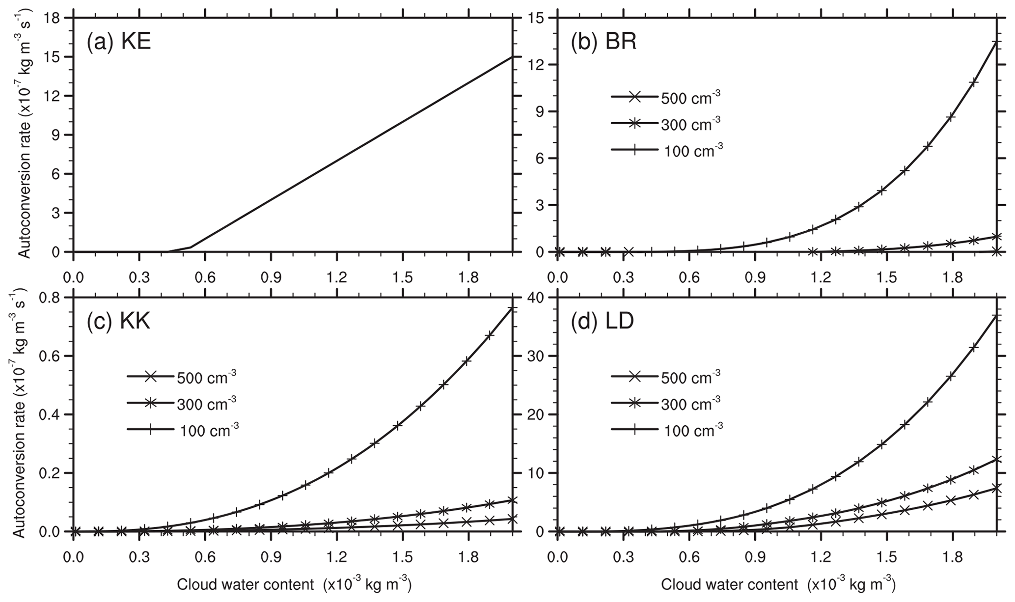
Figure 1Evolution of autoconversion rates with a wide range of cloud water content at given cloud number concentrations (Nc) of 100, 300, and 500 cm−3, respectively. (a) KE denotes the Kessler scheme (1969), and (b) BR indicates the Berry and Reinhardt scheme (1974); (c) KK and (d) LD represent the Khairoutdinov and Kogan (2000) and Liu et al. (LD) schemes (2006), respectively.
2.2 Berry–Reinhardt (BR) scheme
Berry and Reinhardt (1974) proposed a physical formulation to represent the ATC process in clouds, which is given by
Here, µ represents shape parameter of a gamma distribution; ρw is liquid water density. Dmean is the mean diameter (unit in metres) of the total cloud droplets, which is computed from
Here, π is the circumference ratio. The BR scheme was developed theoretically in which not only CWC but also cloud number concentration was incorporated. An important characteristic is that maritime and continental clouds can be differentiated by the BR scheme using different parameters (Simpson and Wiggert, 1969; Pawlowska and Brenguier, 1996). Cotton (1972) argued that the BR scheme seems to underestimate rain formation in their simulations. Compared to KE, the BR scheme has treated the process more rigorously (Ghosh and Jonas, 1999). It should be noted that ATC rates given by BR are quite sensitive to Nc (Fig. 1b).
2.3 Khairoutdinov–Kogan (KK) scheme
Khairoutdinov and Kogan (2000) proposed a computationally efficient and relatively simple scheme, which aims at large-eddy simulation (LES). One of the advantages is that there is no need to define a threshold, and this scheme has been broadly used in numerical models (e.g. Morrison et al., 2009). The ATC rate is given by
The KK scheme uses a simple power-law expression based on a series of large-eddy simulations. Generally speaking, the autoconversion rate increases with increasing CWC and/or decreasing cloud number concentration. The simple expression is a key advantage of the KK scheme, which makes it possible to analytically integrate the microphysical process rates over a probability density function (Griffin and Larson, 2013). In view of Fig. 1c, the KK scheme has a strong dependency on Nc. Increasing Nc from 100 to 500, ATC rates decrease dramatically, especially at the CWCs over 1.0 g m−3. Unlike other schemes, ATC is allowable in the KK scheme even with very low CWCs, which might lead to overestimations under such conditions.
2.4 Liu–Daum–McGraw–Wood (LD) scheme
A generalized ATC parameterization was proposed by Liu et al. (2006). The approach improved the representation of the threshold function by applying the expression for the critical radius derived from the kinetic potential theory. The parameterization is given by
Here, κ ( kg−2 m3 s−1) is a constant. β is a parameter related to the relative dispersion ε of cloud droplets, which is obtained from
Here, a value of 0.5 is assigned to ε following Liu et al. (2006). The LD scheme assumes that autoconversion rate is determined by CWC, cloud number concentration, and relative dispersion of cloud droplets. Xie and Liu (2015) suggested that the LD scheme considering spectral dispersion was more reliable for improving the understanding of the aerosol indirect effects compared to the KE and BR schemes. Note that the LD scheme is characterized by the smooth transition in the vicinity of the ATC threshold.
As has been mentioned above, ATC rates predicted by different schemes can differ by several orders of magnitude for a given CWC. Nowadays, it is still troublesome to judge which scheme is preferred to others at all times (Ghosh and Jonas, 1999; Jing et al., 2019; Liu et al., 2006; Michibata and Takemura, 2015). To the best of our knowledge, each one has its advantages and disadvantages. Keeping this fact in our mind, we propose a weighted (the EN) scheme by employing the above-listed four commonly used ATC schemes, and the weighted ensemble ATC rate (PATC−EN) is given by
Here, wxx, referring to that for KE, KK, LD, and BR, respectively, is the weight of each ATC scheme. It is worth noting that Eq. (7) is easily reduced into any single scheme form by setting all wxx values to 0 except for one of them. Therefore, it is a flexible way to use any one or more schemes to calculate PATC−EN by adjusting wxx. Of course, it is also convenient to reduce the effect of any one of them by giving a small value of wxx. At present, the same weights with the value of 1.0 are assigned for all schemes for simplicity. Note that the weights can be modulated according to weather conditions. One of the features of the EN scheme is that the weighted mean is calculated within a microphysics scheme, and the increase in computation cost is negligible.
Similar to an ensemble prediction system (Lewis, 2005), the EN scheme is expected to reduce the potential uncertainties from the use of any ATC scheme alone under various CWC conditions. For example, no cloud water converts into rainwater in the KS scheme when the cloud water is less than the threshold, while in the KK scheme it always occurs. However, the KS scheme has much higher ATC rates owing to the linear relationship (Eq. 1) compared to those of the KK scheme. Most importantly, the EN scheme is beneficial for the multi-scale numerical weather and climate modelling systems, especially for variable-resolution models (e.g. the Model for Prediction Across Scales, MPAS – Skamarock et al., 2012 – and the Global-to-Regional Integrated forecast SysTem, GRIST – Zhang et al., 2019) because it is flexible to represent cloud processes consistently across all model scales under the various conditions. Depending on grid distance, one or more schemes can be used independently in a variable-resolution model. For example, we assign all wxx to 0 except for wKK in the fine grid distance region, and a mean value from the calculation of two or more schemes is utilized in the grid distance transition zone.
To facilitate comparisons among the aforementioned ATC schemes, an idealized experiment is performed with a wide range of CWCs in the calculations. A rough value of Nc is set to 300 cm−3 in the continental clouds (e.g. Hong and Lim, 2006; Thompson et al., 2008). For convenience, air density is approximately fixed at g cm−3 here. It is noteworthy that the value of 2 is assigned to µ for both BR and LD schemes. Figure 2 compares the EN scheme with the selected four schemes with a wide range of CWCs from 0.01 to 1.0 g m−3. One can see that all the schemes yield ATC rates of g cm−3 s−1, although there are significant discrepancies among the different schemes. For the KS scheme, the ATC of cloud water to rainwater does not start until the CWC exceeds the threshold q0 (Eq. 1). In contrast, the other schemes are allowable even given fair low CWCs.
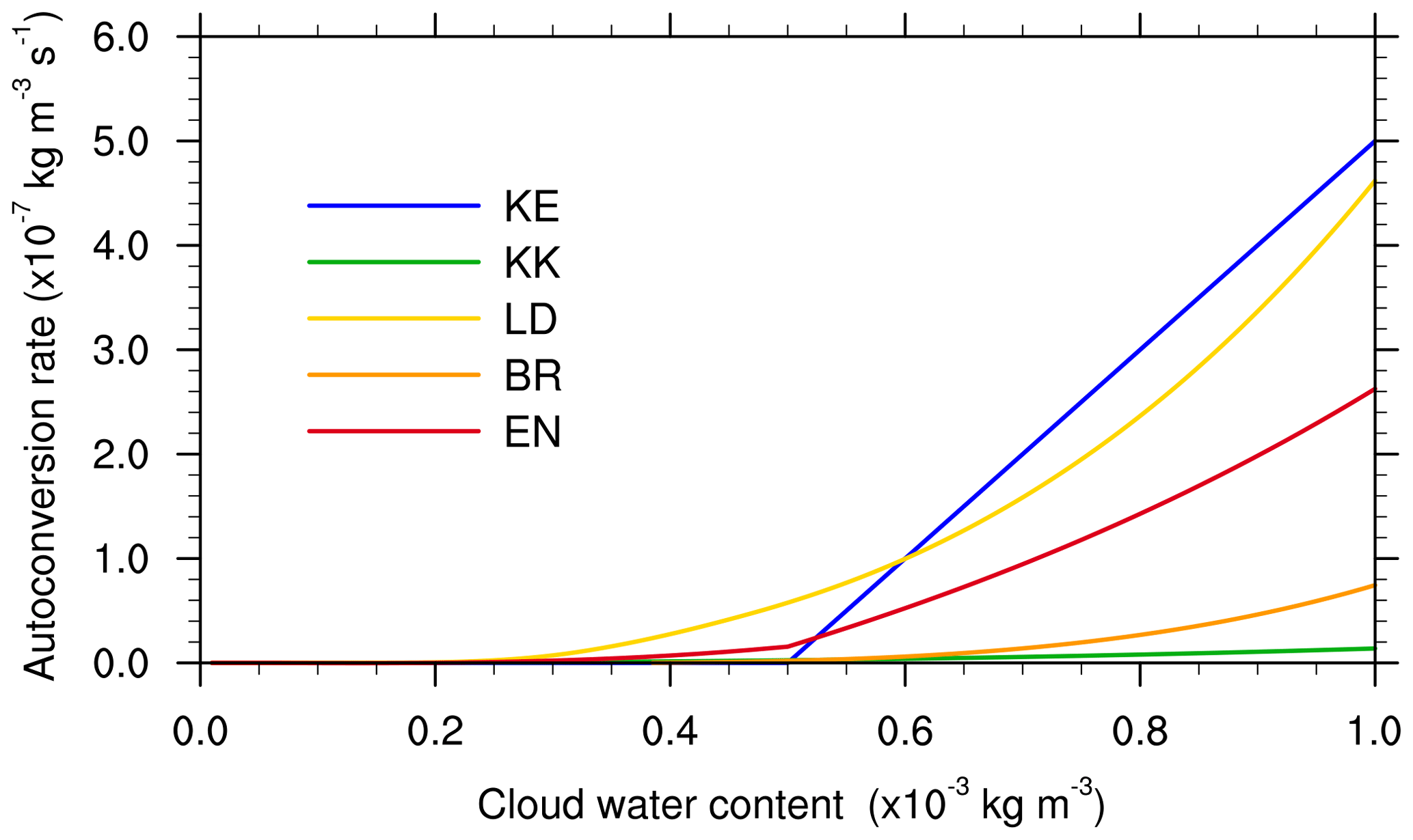
Figure 2Comparisons of the EN scheme with the selected KE, BR, KK, and LD schemes at a fixed Nc of 300 cm−3 (see text for further details).
Comparatively speaking, both KS and LD predict a larger ATC rate than the other ATC schemes (the BR or KK scheme) for a given CWC. As for the former group, LD yields the largest ATC rate with CWC below 0.6 g m−3, while KS generates the largest ATC with CWC over 0.6 g m−3. Wood and Blossey (2005) argued that the ATC rate defined in LD would give the total rate of mass coalescence among cloud droplets and is typically much larger than the true ATC rate. With Nc fixed at 300 cm−3, the BR scheme shows close ATC rates to those of KK. Note that the KK scheme, originally developed for the large-eddy simulation (LES) model, yields the lowest ATC rate, followed by the BR scheme. The EN scheme provides a similar pattern to LD, but nearly half of those ATC rates are yielded by the latter. It should be emphasized that ATC rates are fairly sensitive to Nc (Fig. 1), and a higher or lower Nc would cause great changes.
4.1 Overview of the rainfall event
An extreme rainfall event hit the megacity of Guangzhou in the early morning hours of 7 May 2017. Within 18 h (during the period of 20:00 Beijing Standard Time – BST, – 6 May to 14:00 BST 7 May), there were 12 rain gauge stations over 250 mm during the rainfall process. The spatial distribution of the rainfall yields two heavy rainfall cores over the regions of Jiulong (JL) and Huashan (HS) (Fig. 3a). The event was featured by the heaviest rainfall in the megacity of Guangzhou over the past 6 decades, with the maximum total amount of 542 mm within 18 h at JL station (Fig. 3a). It also broke the record of 3 h accumulated rainfall amount with the value of 382 mm. Another marked feature of this rainfall event was its extreme hourly rainfall rate of 184 mm h−1, which is the second-highest over Guangdong Province, China.
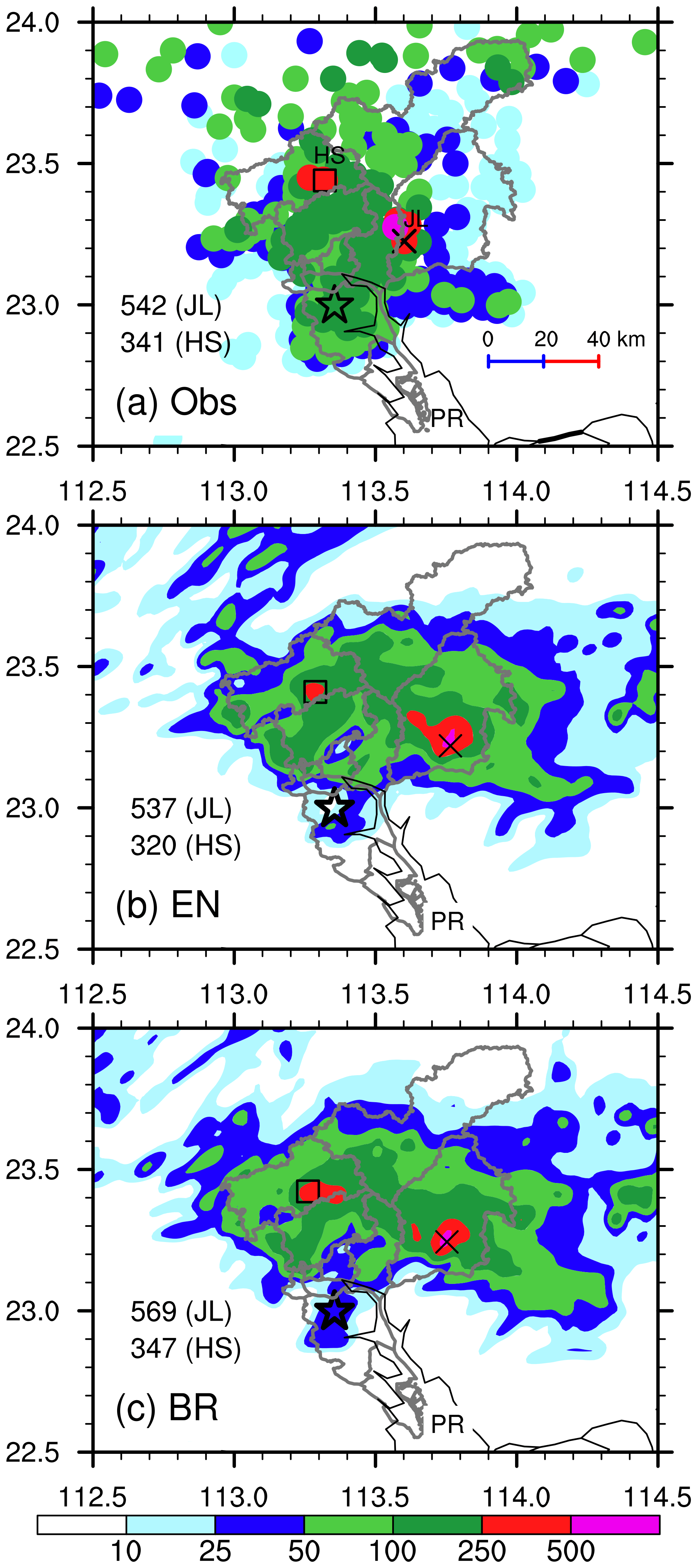
Figure 3Spatial distribution of the 18 h accumulated rainfall during the period of 20:00 BST 6 May to 14:00 BST 7 May 2017: (a) rain gauge observations and (b–c) simulations with the EN and BR autoconversion schemes. A cross sign (×) and a square sign (□) denote the locations where maximum hourly rainfall rates were (a) observed or (b–c) simulated near Jiulong (JL) and Huashan (HS), respectively. The values marked with JL and HS indicate the 18 h maximum accumulated rainfall amounts near JL and HS, respectively. A star indicates the city centre of Guangzhou, and the Pearl River is marked by PR. This notation is used for the rest of the figures.
4.2 Model configuration and experiment settings
This event was well simulated and investigated by Yin et al. (2020), focusing on the effects of urbanization and orography. The WRF model configurations and initial and boundary conditions are the same as Yin et al. (2020) except for updating to the WRF-ARW (v4.1.3) model (Skamarock et al., 2019) with several minor bugs fixed. For convenience, an overview of the WRF model configurations is presented here. The triple-nested domains have x, y dimensions of 313×202, 571×334, and 862×541 with grid sizes of 12, 4, and 1.33 km, respectively. The WRF model physics schemes are configured with the Thompson microphysics scheme (Thompson et al., 2008) with the modifications of the ATC parameterization, the rapid radiative transfer model (rrtm) (Mlawer et al., 1997) for both shortwave and longwave radiative flux calculations, the Yonsei University (YSU) planetary boundary layer (PBL) scheme (Hong et al., 2006), the MM5 Monin–Obukhov scheme for the surface layer (Janjić, 1994), and the Noah-MP land-surface scheme (Niu et al., 2011). The Kain cumulus parameterization scheme (Kain, 2004) is utilized for the outer two coarse-resolution domains but being bypassed in the finest domain. All the three nested domains of the WRF model are integrated for 18 h, starting from 20:00 BST 6 May 2017, with outputs at 6 min intervals. The initial and outermost boundary conditions are interpolated from the National Centers for Environmental Prediction (NCEP) Global Forecast System 0.25∘ reanalysis data at 6 h intervals. In order to introduce realistically the urban heat island (UHI) effects of the Guangzhou metropolitan region, the four-dimension data assimilation (FDDA) functions are activated (Reen, 2016) by performing both the surface observation nudging and the analysis nudging from 20:00 BST 6 May to 08:00 BST 7 May 2017. Please refer to Yin et al. (2020) for more details about the model configuration.
As has been addressed above, it is convenient to conduct a simulation with any of the above-listed ATC schemes alone. In total, two experiments were carried out with the EN and BR schemes. It should be noted that the BR scheme was used originally in the Thompson scheme, and the EN was newly coupled into the Thompson scheme in this work.
5.1 Spatial distribution of accumulated rainfall
Figure 3 compares the spatial distribution of 18 h simulated total rainfall from the simulations with the EN and BR schemes to the observed. Generally speaking, both schemes are able to capture the main characteristics of the extreme rainfall event. One can see that the simulated rainfall amount compares favourably to the observed at both HS and JL, although the JL storm has a 10–15 km eastward location shift. Yin et al. (2020) argued that the location errors may be related to large-scale meteorological conditions. Comparatively speaking, the EN and BR schemes performed better than others. The two centralized rainfall cores over HS and JL were successfully captured by the EN and BR schemes, with a simulated heaviest rainfall amount of 537 and 569 mm, respectively (Fig. 3b and c). As for the EN scheme (Fig. 3b), the simulated 18 h total rainfalls were 320 and 537 mm over HS and JL, respectively, which was close to the observations of 341 and 542 mm (Fig. 3a). Similarly, the BR scheme performed equivalently to the EN scheme, with a maximum rainfall of 347 and 569 mm over Huashan and Jiulong regions, respectively (Fig. 3c). Note that the simulated heaviest rainfalls over the Huashan region were comparative among each other. In view of the results, we compare the maximum hourly rainfall rates near JL from the simulations of the EN and BR schemes to those of observations in the next sections. It should be noted that the results in the present study are a little better than (or equivalent to at least) those in Yin et al. (2020) because of the update of the WRF version 4.1.3 model with some improvements in dynamical framework and bug fixes.
5.2 Evolution of the simulated hourly rainfall
Figure 4 shows the observed and simulated time series of hourly maximum rainfall rates over the Jiulong region. The observed peak rainfall near JL occurred at 06:00 BST 7 May with the hourly rates of 184 mm h−1. However, the simulated peak rainfall from the EN scheme took place at 07:00 BST 7 May, which was about 1 h later than the observed, with hourly rates of 151 mm h−1. As for the BR scheme, the simulated peak rainfall rate occurred 2 h later, with a value of 144 mm h−1. As a matter of fact, both EN and BR schemes underpredicted the peak hourly rainfall rate near JL. It is worthy to note that the observed timings of initiating and ending of the extreme rainfall production episode, i.e. near 03:00 and 10:00 BST 7 May, respectively, were reproduced successfully. However, both simulated peak rates occurred later than the observed due to the slower increases in rain-producing rates than the observed. More specifically, the observed hourly rate increased from about 16 to 184 mm h−1 in just 1 h (i.e. from 05:00 to 06:00 BST). However, the simulated hourly rate from the EN scheme increased from 0.3 mm h−1 at 04:00 BST to about 79 mm h−1 at 06:00 BST and then to 151 mm h−1 at 07:00 BST 7 May. As for the simulated hourly rate with the BR scheme, it increased from 2 mm h−1 at 04:00 BST to about 104 mm h−1 at 07:00 BST and then to 144 mm h−1 at 08:00 BST 7 May. One unique feature of the observations was the rapid increase in the hourly rainfall rate. The rainfall produced by the EN scheme peaked within 2 h, while the BR scheme peaked over a period of 4 h. Additionally, both the simulated rainfall rates decrease for several hours. Generally speaking, the EN scheme performed much closer to the observed, compared to that of the BR scheme. Note that the longer heavy rainfall period from the BR scheme contributed partially to the overprediction of the 18 h accumulated rainfall (Fig. 3c).
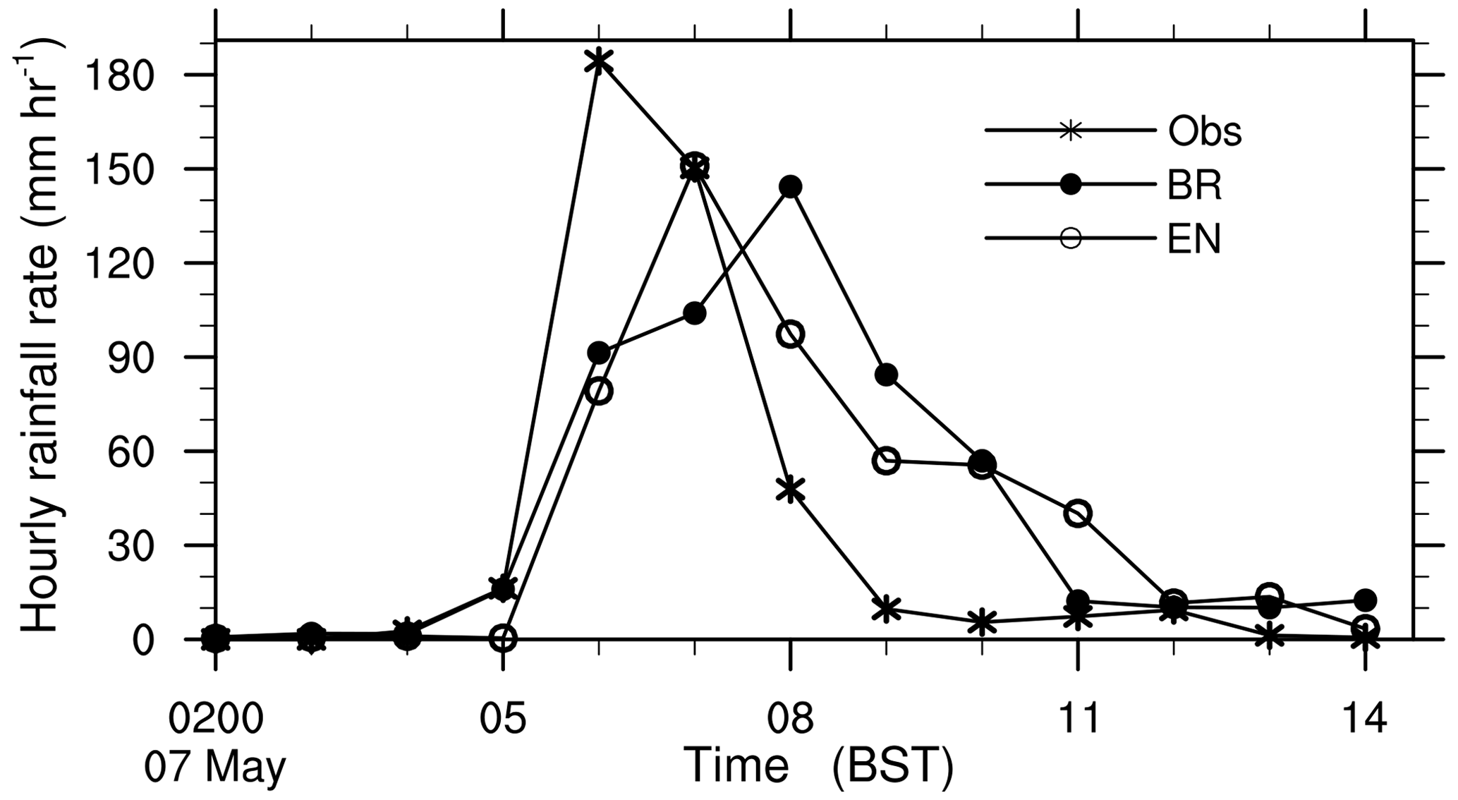
Figure 4Time series of hourly rainfall rates (mm h−1) from rain gauge observations (*) and simulated with the EN scheme (∘) and the BR scheme (•) near Jiulong during the period of 20:00 BST 6 May–14:00 BST 7 May 2017 (see Fig. 3 for their locations).
5.3 Evolutions of radar reflectivity
In view of the performance of the accumulated rainfall and the maximum hourly rainfall rates, we only compare the radar reflectivity from the simulations with the EN scheme to the results of the BR scheme. Figure 5 exhibits the structures and evolutions of convective cells over the JL region by comparing the simulated composite radar reflectivity to the observed. The first well-organized radar echo formed near 00:00 BST over the Huashan region (not shown), which was located at the northern edge of a surface high-θe (equivalent potential temperature) tongue with significant convergence. As the south-easterly flow moved slowly eastward, and the cold outflows resulted from previous convection, the Huashan storm dissipated, while the storm began to develop over the Jiulong region, in both its size and intensity (Fig. 5a). The storm rapidly intensified during the period from 04:30 to 05:30 BST, with the peak reflectivity beyond 55 dBZ near the leading edge (Fig. 5a and b). The Jiulong storm moved fairly slowly, keeping more or less quasi-stationary shortly after its formation (Fig. 5a–c). Both the quasi-stationary nature and intense radar reflectivity explain the extreme rainfall production rate occurring at JL during the 1 h period of 05:00–06:00 BST. Subsequently, the Jiulong storm weakened, but its associated peak radar reflectivity still remained over 50 dBZ, which was consistent with the continued generation of significant rainfall near JL until 08:00 BST (Fig. 4).
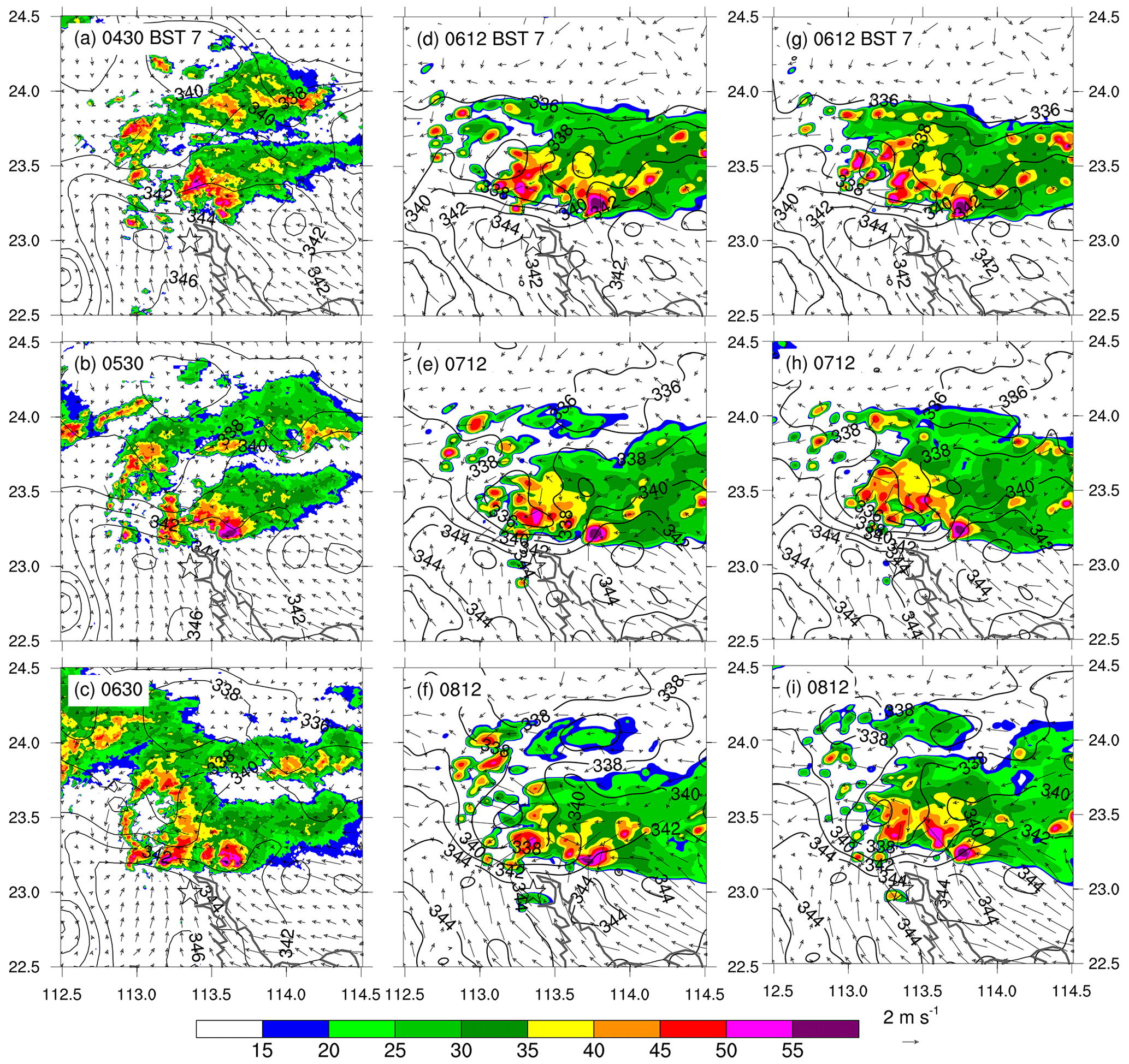
Figure 5Horizontal maps of composite radar reflectivity (dBZ; shadings) and surface (z=10 m) horizontal wind vectors and equivalent potential temperature (θe; contoured at 2 K intervals) during the extreme rainfall stage: (a–c) observed, (d–f) simulated with the EN scheme, and (g–i) simulated with the BR scheme. A reference wind vector is given beneath the right column next to the composite radar reflectivity colour scale.
It is obvious that both the EN and BR schemes captured the development of the Jiulong storm, with main features that were similar to the observed, including quasi-stationary nature, south-eastward expansion, and concentrated strong radar reflectivity during the extreme rainfall stage. Both simulations successfully generated a lower-θe pool with a distinct outflow boundary interacting with the moist south-easterly flow near the ground. It should be noted that the initiation and organization of both simulated Jiulong storms were about 1.7 h later than the observed, and it occurred at a location nearly 10–15 km to the east of the observed one. Generally speaking, both simulations with the EN and BR schemes produced extreme rainfall amounts close to those observed, and their spatial distributions agree well with observations.
In terms of the spatial distribution of radar reflectivity, similar patterns can be seen between the EN and BR schemes in the early stage before 07:12 UTC, while differences are visible at the extreme rainfall stage (Fig. 5e and h). One can find that the Jiulong storm simulated with the EN scheme (Fig. 5f) developed more rapidly than that from the BR scheme, almost 1 h earlier than the latter (Fig. 5i). This was consistent with the timing lag in the hourly extreme rainfall production (Fig. 4). Clearly, the ACT process has an important influence on the convective development of deep convection associated with the extreme rainfall produced within the Jiulong storm, which is explored in view of the cloud microphysical processes in the next section.
5.4 The effects on macro- and micro-physical processes
The spatial distribution of hourly rainfall and temporally averaged surface temperature and horizontal wind during the period from 06:00 to 07:00 BST from the simulations with the EN and BR schemes are displayed in Fig. 6. As has been stated above, the total rainfall shows a slight difference between EN and BR over the Jiulong region (Fig. 3b and c). In view of the spatial distribution of the hourly rainfall during the period when maximum hourly rainfall occurred (i.e. 06:00 to 07:00 BST 7 May 2017; Fig. 6), the EN scheme generated a larger rainfall area and a stronger rainfall rate than those of the BR scheme, although both schemes produced similar spatial distribution patterns in rainfall area and temporally averaged surface temperature and horizontal wind field. The result was consistent with the idealized experiments given in Fig. 2. For a given CWC, the EN scheme had a larger ATC rate compared to the BR scheme, and the difference becomes obvious with the increase in CWC. Consequently, the EN scheme produced more rainwater of small to middle size compared to the BR scheme. The larger rainwater was favourable for the coalescence of large precipitation particles from the upper levels, which made the larger contribution to the extreme rainfall rate. This is why the EN scheme produced larger rainfall than the BR scheme. The result was consistent with Fu and Lin (2019), in which the autoconversion threshold limited the temporal and spatial extent of the “vigorous rain formation region” where most of the rain was produced. Those features can also be viewed from the vertical sections in Fig. 7. One can see that the largest radar reflectivity reaches the ground, like a bell on the ground (Fig. 7a). This unique feature was reported by Li et al. (2020) based on the observations from the S-band dual-polarization radar at Guangzhou station, Guangdong Province, China. The bell-shaped radar reflectivity was consistent with the episode of the extreme hourly rainfall. The strong radar reflectivity mainly resulted from raindrop coalescence owing to the higher raindrop number concentration in the lower levels (Bao et al., 2020). That is to say, collecting rainwater by the collision–coalescence process at the lower levels helped create a large rainfall rate at the ground. As for the BR scheme (Fig. 7b), a middle-level radar reflectivity core was obvious above nearly 1 km up to 4 km, indicating that raindrop coalescence occurred intensively between those levels, and evaporation of raindrops was significant below 1 km. The evaporation near the surface was a considerable factor abating the surface rainfall rate. In view of the vertical distribution of radar reflectivity, the EN scheme generated a maritime-like convective storm, whereas the convective storm simulated by the BR scheme was close to continental-like convection. It should be noted that except for evaporation, large particle (raindrop) breakup can lead reflectivity values to decrease toward the surface because reflectivity is very sensitive to raindrop size. In the present case, the evaporation of raindrops was remarkable. However, a slight difference was found in differential reflectivity ZDR in the lower levels, indicating that large particle (raindrop) breakup was weak.
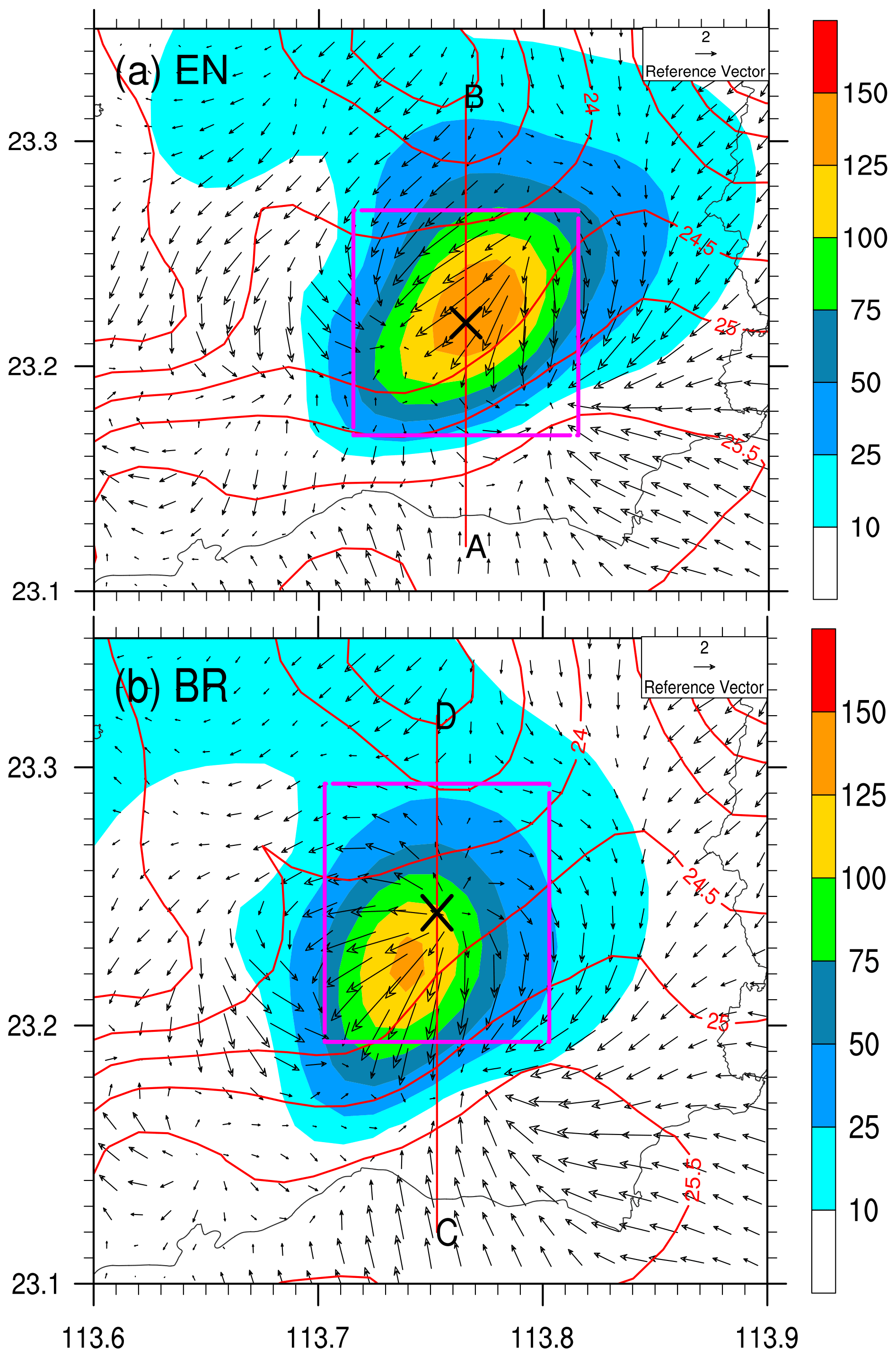
Figure 6Spatial distribution of hourly rainfall amount (mm; shadings), temporally averaged surface temperature (contoured at 0.5 ∘C intervals), and horizontal wind fields (vectors) during the period from 06:00 to 07:00 BST 7 May 2017. The red lines, A–B (a) and C–D (b), indicate the locations of the vertical cross-section in Fig. 7. The two pink square boxes, covering an area of with the centre of the maximum hourly rainfall, are marked for domain-averaged calculation in Figs. 8 and 9.
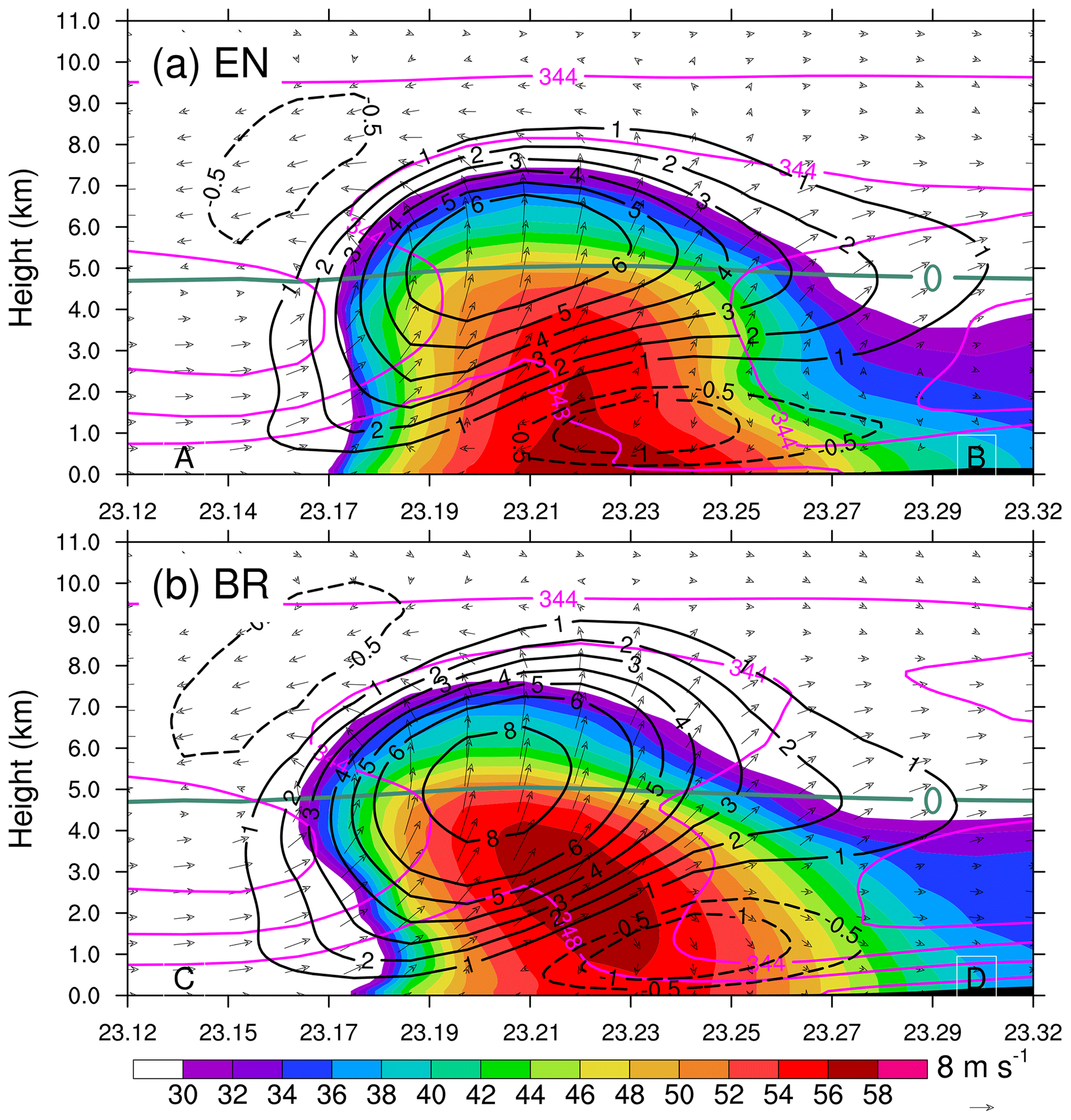
Figure 7Temporally averaged vertical cross-sections along (a) A–B and (b) C–D in Fig. 6 of the simulated reflectivity (dBZ; shadings), vertical velocity (black contours; m s−1), in-plane flow vectors (vertical motion amplified by a factor of 2), and θe (pink-contoured at 4 K intervals) during the period from 06:00 to 07:00 BST 7 May 2017. The thick light-green line indicates an isotherm of 0 ∘C.
Both the EN and BR schemes provide tilted storms in view of vertical crossing from the south to north through the extreme rainfall. During this episode, the updraught was dominant in the storm, and a weak downdraught occurred in the lower levels at the back of the convective storm. Besides, both EN and BR reproduced very close thermal patterns in terms of potential temperature. Note that the EN scheme had a slightly weaker updraught than that of the BR scheme, although the modifications to the ATC parameterization are only made in the microphysics scheme (Fig. 7a and b), suggesting that change in cloud microphysical processes can lead to some variations in dynamical processes.
The differences between the EN scheme and BR schemes in updraught can be also viewed from the cumulative contoured frequency by altitude diagrams (CCFADs) given in Fig. 8. CCFAD presents the percentage of horizontal grid points with vertical motion weaker than the abscissa scaled value for a given height (Yuter and Houze, 1995). In this study, vertical speeds are binned with intervals of 1 m s−1 based on the 11 model outputs with 6 min intervals during the severe rainfall episode from 06:00 to 07:00 BST 7 May 2017. Generally speaking, the EN scheme shows similar CCFAD patterns to those of the BR scheme. However, there are still differences in the vertical motion. One can see there was a slightly weaker core, which is lower in the EN scheme simulation compared to those of the BR scheme. During the severe rainfall episode, the EN scheme produced the largest updraught of nearly 15 m s−1 at the 5 km level, while that was about 16 m s−1 at the 6 km level given by the BR scheme. In contrast, updraughts below 6 m s−1 occurred more frequently in EN than that in the BR scheme. Overall, the EN scheme provided a larger updraught area, which is however weaker in upward speed compared to those in the BR scheme. This is why the EN scheme had a larger spatial distribution of rainfall than that of the BR scheme (Fig. 6a and b). Note that both EN and BR schemes had a slight difference in downdraughts in vertical distribution, and the downdraught was mainly located below 2 km, which was also visible in the vertical cross-sections (Fig. 7a and b).
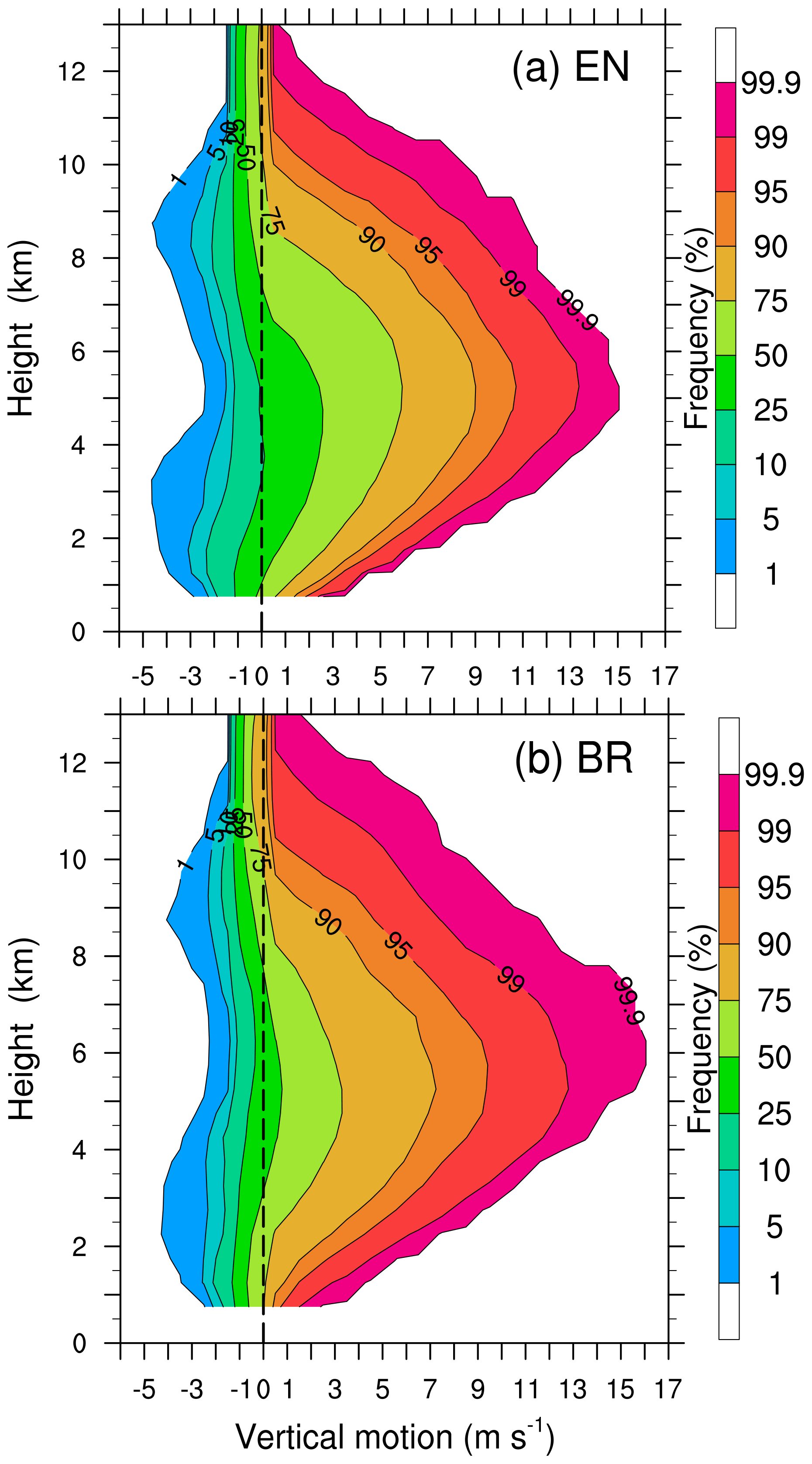
Figure 8CCFADs of the simulated vertical motion for (a) the EN scheme and (b) the BR scheme within the respective boxes marked with pink lines in Fig. 6. The CCFADs are calculated from 11 model outputs with 6 min intervals during the severe rainfall episode from 06:00 to 07:00 BST 7 May 2017.
As is noted above, both the EN and BR schemes produced very close dynamical patterns except for updraughts. However, differences were remarkable in cloud microphysical processes. Figure 9 compares the temporal evolution of hydrometeors between the EN and BR schemes. One can see that the EN scheme (Fig. 9a–f) produced similar hydrometeor patterns to those of the BR scheme (Fig. 9g–i). Overall, graupel was dominant above the melting layer, while rainwater was considerable below the melting layer. Previous studies (Franklin et al., 2005; Krueger et al., 1995; McCumber et al., 1991; Yin et al., 2018) proposed that graupel was dominant in the tropical and subtropical clouds owing to plentiful water vapour. Overall, the EN scheme mainly increased rainwater content and graupel, with only slight differences in cloud water, cloud ice, snow, and water vapour compared with those of the BR scheme (Fig. 9m–r).

Figure 9Comparison of time–height cross-sections of domain-averaged mixing ratios between the EN scheme (a–f) and the BR scheme (g–i) during the period from 06:00 to 07:00 BST 7 May 2017 within the domains marked with pink lines in Fig. 6; qc, qr, qi, qs, and qg denote cloud water, rainwater, cloud ice, snow, and graupel, respectively. Panels (m)–(r) give the differences between EN and BR (i.e, EN−BR). Thick blue lines indicate an isotherm of −15 and 0 ∘C, respectively.
In terms of the difference in rainwater and graupel between the EN and the BR schemes (Fig. 9m–r), we find that the ATC rate of the EN scheme played an important role in the development of deep convection. Compared to the BR scheme, the higher ATC rate of the EN scheme quickly produced a more considerable number of small precipitation-sized drops within updraughts in moderate and lower levels, and more of the small-sized raindrops were lofted by the updraughts above the 0 ∘C level and subsequently were fed for ice processes. Within this, graupel coexisted with more small-sized supercooled raindrops, and stronger riming occurred between ice particles and the small-sized raindrops. Consequently, more of the small supercooled raindrops were converted into graupel by ice cloud microphysical processes such as riming, leading to a more rapid graupel production. At the same time (Fig. 9q), more supercooled raindrops froze, becoming more graupel embryos since bigger raindrops freeze at warmer temperatures than smaller cloud droplets and continue to grow by riming and/or other processes. Consequently, graupel was increased at high altitude (above 0 ∘C) levels. It is well known that bigger water drops freeze at warmer temperatures than small drops. Therefore, the small raindrops partially froze into graupel and snow particles, which contributes to the increment in graupel and snow. Generally, a graupel particle has a larger size than a raindrop with a given mass. Therefore, the larger graupel particle can collect more particles as they fall down in the storm, which helped create the surface heavy rainfall rate. One can see that the graupel increased rapidly nearly 12 min after the appearance of increasing supercooled rain (Fig. 9n). It should be noted that we try to understand cloud microphysical processes in the extreme rainfall based on our knowledge at present, and thus a rigorous validation is required by comparing hydrometeors' sink and terms in a future study.
As the increased graupel passed by the melting level, they started to melt, leading to more raindrops. In view of the strong radar reflectivity near the surface in Fig. 7a, the raindrops from upper levels grew rapidly by collecting raindrops in the lower levels. In this way, the extreme rainfall rate was generated in such a more rapid and efficient approach compared to those of the BR scheme. During this stage, the increased ATC rate was linked to ice-phase processes and modified graupel fraction in the upper levels above 0 ∘C. As has been mentioned earlier, the increased ATC rate played a certain role in dynamic feedbacks, and the degree of modulation of water vapour, cloud water, cloud ice, and snow by the increased ATC rate was negligible. These findings indicate that increased ATC rate was important in the extreme rainfall that involved ice-phase processes of graupel above the 0 ∘C levels and warm-rain processes of raindrops in the lower levels. To summarize, the higher ATC rate of the EN scheme produced more small precipitation-sized drops, and some of the small-sized raindrops were lofted to the upper levels above 0 ∘C. Consequently, more graupel was generated by riming and freezing processes. The rapid production of graupel played a significant role in the development of extreme rainfall. Collision and coalescence processes between liquid particles appeared to be the mechanism of radar reflectivity increment toward the surface within the storm's core region.
We proposed the influence mechanism of the ATC rate on the extreme rainfall by comparing the simulated results between the EN scheme and the BR scheme. However, there are still some limitations in figuring out the complete effects of the increasing ATC rate on microphysical and dynamical processes at present because those processes are entangled with complicated interactions. Therefore, a better choice is to separate the effects on each process by conducting high-resolution simulations with a sophisticated model, such as the approach of Grabowski (2014). Certainly, the best way is to perform offline testing based on in situ observations, as was done by Wood (2005). Keeping those issues in our mind, further work is needed to address this question.
In this study, we designed an ensemble (EN) approach to improving ATC process description in the cloud microphysics schemes. One unique feature of the EN approach is that the ATC rate is a mean value based on the calculations from several widely used ATC schemes. Similar to ensemble prediction, this approach is aimed to improve the representation of the ATC rate in case it has been treated by using an ATC scheme alone in the cloud microphysics schemes. At present, the four widely used ATC schemes are selected, including the Kessler (1969) scheme, the Berry and Reinhardt (1974) scheme, the Khairoutdinov and Kogan (2000) scheme, and the Liu et al. (2006) scheme. In the EN scheme, each scheme is assigned a weight (Eq. 7) in order to modulate its importance. Certainly, the EN scheme is easily reduced into any single scheme by setting all wxx values to 0 except for one of them. It is also convenient to reduce the effect of a scheme by giving a small value of wxx and even removing the effect of a scheme by assigning a value of weight to 0. Under this framework, the ATC rates from the EN scheme are compared to those from each of the several commonly used schemes by ideal experiments, and a series of simulations are carried out for an urban-induced extreme rainfall event over southern China by using the EN, KE, BR, KK, and LD schemes, which are coupled into the Thompson scheme in the WRF model (Thompson et al., 2008) in this work. The results show that the EN scheme provides better simulations compared to those from any single ATC scheme used alone.
In this study, the ensemble approach has been employed to represent the ATC process in the Thompson cloud microphysics scheme, which shows some advantages for simulation of the extreme rainfall event that occurred on 7 May 2017 over southern China. It is important to acknowledge that the conclusions are drawn from just one case study and have not been validated under a wider range of conditions over the world. In the forthcoming studies, a systematic assessment of heavier rainfall events is planned to better understand the performance of the EN scheme. It should be noted that there are still some limitations to the EN scheme in the present study. Although a large number of ATC schemes are available, most among them are not employed as ensemble members. For example, the Franklin scheme (Franklin, 2008) took the effect of turbulence on the ATC process into account, which plays an important role in precipitation development (Chandrakar et al., 2018; Seifert et al., 2010). Furthermore, equal weights were used in the present study for convenience. In other words, the selected schemes have the same effect on the ATC rate. Moreover, only conventional verifications were carried out, and the dependency of the performance of the ATC schemes on the model resolution was not considered in this study. A further examination with new approaches (e.g. Wood, 2005; Grabowski, 2014) might provide important insights in the near future.
ATC is an important process of raindrop initiation in the low-level clouds in general circulation models (GCMs) and has remarkable effects on the models' results (e.g. Golaz et al., 2011; Roy et al., 2021). The ATC is sensitive to an ATC scheme, even a parameter, due to heterogeneous cloud properties over the world. Consequently, the EN scheme may be a good option for GCMs in which there are various possible cloud conditions. It is worth emphasizing that we focus our attention on the ATC from cloud water into rainwater at present. Certainly, any source or sink term in a cloud microphysics scheme can be dealt with using the same method. Since developing a “unified” cloud scheme appears to be a significant part of weather and climate model development in the coming years (Randall et al., 2019), the EN approach may be a practicable way to reduce the potential uncertainty in cloud and precipitation physical processes, which will contribute to more accurate numerical model development.
The source code of the Weather Research and Forecasting model (WRF v4.1.3) is available at https://doi.org/10.5065/D6MK6B4K (Skamarock et al., 2019). Modified WRF model codes and initial and boundary data used for the simulations are available on Zenodo (https://doi.org/10.5281/zenodo.5052639; Yin et al., 2021). The National Centers for Environmental Prediction (NCEP) Global Forecast System 0.25∘ final analysis data at 6 h intervals used for the initial and boundary conditions for the specific analysed period can be downloaded at https://doi.org/10.5065/D65Q4T4Z (National Centers for Environmental Prediction/National Weather Service/NOAA/U.S. Department of Commerce, 2015).
JY developed the weighted ensemble scheme and coupled the scheme into the WRF model, with contributions from XL. JY tested and verified the scheme with contributions from XL, HW, and HX. JY wrote the manuscript, and all the authors continuously discussed the results and contributed to the improvement of the paper.
The contact author has declared that neither they nor their co-authors have any competing interests.
Publisher’s note: Copernicus Publications remains neutral with regard to jurisdictional claims in published maps and institutional affiliations.
The authors acknowledge the use of the NCAR Command Language (NCL) in the analysis of some of the WRF Model output and the preparation of figures. The authors are thankful to the chief editor (Astrid Kerkweg), the handling topical editor (David Topping), and the two anonymous reviewers for their help in improving the manuscript.
This research has been supported by the National Key Research and Development Program of China (grant nos. 2018YFC1507404 and 2017YFC1501806), and the National Natural Science Foundation of China (grant no. 42075083)
This paper was edited by David Topping and reviewed by two anonymous referees.
Bao, X., Wu, L., Zhang, S., Li, Q., Lin, L., Zhao, B., Wu, D., Xia, W., and Xu, B.: Distinct Raindrop Size Distributions of Convective Inner- and Outer-Rainband Rain in Typhoon Maria (2018), J. Geophys. Res.-Atmos., 125, e2020JD032482, https://doi.org/10.1029/2020JD032482, 2020.
Beheng, K. D.: A parameterization of warm cloud microphysical conversion processes, Atmos. Res., 33, 193–206, https://doi.org/10.1016/0169-8095(94)90020-5, 1994.
Berry, E. X.: Modification of the warm rain process, Preprints, First National Conference on Weather Modification, Albany, NY, USA, 28 April–1 May, B. Am. Meteorol. Soc., 81–88, http://merlin.lib.umsystem.edu/record=b1539470~S1 (last access: January 2022), 1968.
Berry, E. X. and Reinhardt, R. L.: An Analysis of Cloud Drop Growth by Collection Part II. Single Initial Distributions, J. Atmos. Sci., 31, 1825–1831, https://doi.org/10.1175/1520-0469(1974)031<1825:aaocdg>2.0.co;2, 1974.
Caro, D., Wobrock, W., Flossmann, A. I., and Chaumerliac, N.: A two-moment parameterization of aerosol nucleation and impaction scavenging for a warm cloud microphysics: description and results from a two-dimensional simulation, Atmos. Res., 70, 171–208, https://doi.org/10.1016/j.atmosres.2004.01.002, 2004.
Chandrakar, K. K., Cantrell, W., and Shaw, R. A.: Influence of Turbulent Fluctuations on Cloud Droplet Size Dispersion and Aerosol Indirect Effects, J. Atmos. Sci., 75, 3191–3209, https://doi.org/10.1175/JAS-D-18-0006.1, 2018.
Chen, S.-H. and Sun, W.-Y.: A One-dimensional Time Dependent Cloud Model, J. Meteorol. Soc. Jpn., 80, 99–118, https://doi.org/10.2151/jmsj.80.99, 2002.
Cotton, W. R.: Numerical Simulation of Precipitation Development in Supercooled Cumuli – Part I, Mon. Weather Rev., 100, 757–763, https://doi.org/10.1175/1520-0493(1972)100<0757:NSOPDI>2.3.CO;2, 1972.
Doswell, C. A.: Severe Convective Storms – An Overview, Meteor. Mon., 50, 1–26, https://doi.org/10.1175/0065-9401-28.50.1, 2001.
Dudhia, J.: Numerical Study of Convection Observed during the Winter Monsoon Experiment Using a Mesoscale Two-Dimensional Model, J. Atmos. Sci., 46, 3077–3107, https://doi.org/10.1175/1520-0469(1989)046<3077:NSOCOD>2.0.CO;2, 1989.
Falk, N. M., Igel, A. L., and Igel, M. R.: The relative impact of ice fall speeds and microphysics parameterization complexity on supercell evolution, Mon. Weather Rev., 147, 2403–2415, https://doi.org/10.1175/MWR-D-18-0417.1, 2019.
Flatøy, F.: Comparison of two parameterization schemes for cloud and precipitation processes, Tellus A, 44, 41–53, https://doi.org/10.3402/tellusa.v44i1.14942, 1992.
Franklin, C. N.: A Warm Rain Microphysics Parameterization that Includes the Effect of Turbulence, J. Atmos. Sci., 65, 1795–1816, https://doi.org/10.1175/2007JAS2556.1, 2008.
Franklin, C. N., Holland, G. J., and May, P. T.: Sensitivity of Tropical Cyclone Rainbands to Ice-Phase Microphysics, Mon. Weather Rev., 133, 2473–2493, https://doi.org/10.1175/MWR2989.1, 2005.
Freeman, S. W., Igel, A. L., and van den Heever, S. C.: Relative sensitivities of simulated rainfall to fixed shape parameters and collection efficiencies, Q. J. Roy. Meteor. Soc., 145, 2181–2201, https://doi.org/10.1002/qj.3550, 2019.
Fu, H. and Lin, Y.: A Kinematic Model for Understanding Rain Formation Efficiency of a Convective Cell, J. Adv. Model. Earth Sy., 11, 4395–4422, https://doi.org/10.1029/2019MS001707, 2019.
Ghosh, S. and Jonas, P. R.: On the application of the classic Kessler and Berry schemes in Large Eddy Simulation models with a particular emphasis on cloud autoconversion, the onset time of precipitation and droplet evaporation, Ann. Geophys., 16, 628–637, https://doi.org/10.1007/s00585-998-0628-2, 1999.
Gilmore, M. S. and Straka, J. M.: The Berry and Reinhardt Autoconversion Parameterization: A Digest, J. Appl. Meteorol. Clim., 47, 375–396, https://doi.org/10.1175/2007JAMC1573.1, 2008.
Gilmore, M. S., Straka, J. M., and Rasmussen, E. N.: Precipitation uncertainty due to variations in precipitation particle parameters within a simple microphysics scheme, Mon. Weather Rev., 132, 2610–2627, https://doi.org/10.1175/MWR2810.1, 2004.
Grabowski, W. W.: Extracting Microphysical Impacts in Large-Eddy Simulations of Shallow Convection, J. Atmos. Sci., 71, 4493–4499, https://doi.org/10.1175/JAS-D-14-0231.1, 2014.
Grabowski, W. W., Wu, X., and Moncrieff, M. W.: Cloud Resolving Modeling of Tropical Cloud Systems during Phase III of GATE. Part III: Effects of Cloud Microphysics, J. Atmos. Sci., 56, 2384–2402, https://doi.org/10.1175/1520-0469(1999)056<2384:CRMOTC>2.0.CO;2, 1999.
Grabowski, W. W., Morrison, H., Shima, S.-I., Abade, G. C., Dziekan, P., and Pawlowska, H.: Modeling of Cloud Microphysics: Can We Do Better?, B. Am. Meteorol. Soc., 100, 655–672, https://doi.org/10.1175/BAMS-D-18-0005.1, 2019.
Griffin, B. M. and Larson, V. E.: Analytic upscaling of a local microphysics scheme. Part II: Simulations, Q. J. Roy. Meteor. Soc., 139, 58–69, https://doi.org/10.1002/qj.1966, 2013.
Hong, S.-Y., Noh, Y., and Dudhia, J.: A new vertical diffusion package with an explicit treatment of entrainment processes, Mon. Weather Rev., 134, 2318–2341, https://doi.org/10.1175/MWR3199.1, 2006.
Houghton, J. T., Ding, Y. H., Griggs, D. J., Noguer, M., van der Linden, P. J., Dai, X., Maskell, K., and Johnson, C. A. (Eds.): Climate Change 2001: The Scientific Basis, Cambridge University Press, Cambridge, 49 pp., 052-1014956, 2001.
Hsieh, W. C., Jonsson, H., Wang, L. P., Buzorius, G., Flagan, R. C., Seinfeld, J. H., and Nenes, A.: On the representation of droplet coalescence and autoconversion: Evaluation using ambient cloud droplet size distributions, J. Geophys. Res.-Atmos., 114, D07201, https://doi.org/10.1029/2008JD010502, 2009.
Iacobellis, S. F. and Somerville, R. C. J.: Evaluating parameterizations of the autoconversion process using a single-column model and Atmospheric Radiation Measurement Program measurements, J. Geophys. Res.-Atmos., 111, D02203, https://doi.org/10.1029/2005jd006296, 2006.
Janjić, Z. I.: The step-mountain eta coordinate model: further developments of the convection, viscous sublayer, and turbulence closure schemes, Mon. Weather Rev., 122, 927–945, https://doi.org/10.1175/1520-0493(1994)122<0927:TSMECM>2.0.CO;2, 1994.
Jing, X., Suzuki, K., and Michibata, T.: The Key Role of Warm Rain Parameterization in Determining the Aerosol Indirect Effect in a Global Climate Model, J. Climate, 32, 4409–4430, https://doi.org/10.1175/JCLI-D-18-0789.1, 2019.
Kain, J. S.: The Kain–Fritsch Convective Parameterization: An Update, J. Appl. Meteorol., 43, 170–181, https://doi.org/10.1175/1520-0450(2004)043<0170:TKCPAU>2.0.CO;2, 2004.
Kessler, E.: On the Distribution and Continuity of Water Substance in Atmospheric Circulations, Meteor. Mon., 10, American Meteorological Society, Boston, MA, USA, ISBN 978-1-935704-36-2, 1969.
Khain, A. P., Beheng, K. D., Heymsfield, A., Korolev, A., Krichak, S. O., Levin, Z., Pinsky, M., Phillips, V., Prabhakaran, T., Teller, A., van den Heever, S. C., and Yano, J. I.: Representation of microphysical processes in cloud-resolving models: Spectral (bin) microphysics versus bulk parameterization, Rev. Geophys., 53, 2014RG000468, https://doi.org/10.1002/2014RG000468, 2015.
Khairoutdinov, M. and Kogan, Y.: A New Cloud Physics Parameterization in a Large-Eddy Simulation Model of Marine Stratocumulus, Mon. Weather Rev., 128, 229–243, https://doi.org/10.1175/1520-0493(2000)128<0229:ANCPPI>2.0.CO;2, 2000.
Kogan, Y. and Ovchinnikov, M.: Formulation of Autoconversion and Drop Spectra Shape in Shallow Cumulus Clouds, J. Atmos. Sci., 77, 711–722, https://doi.org/10.1175/JAS-D-19-0134.1, 2019.
Kong, F. and Yau, M. K.: An explicit approach to microphysics in MC2, Atmos. Ocean, 35, 257–291, https://doi.org/10.1080/07055900.1997.9649594, 1997.
Krueger, S. K., Fu, Q., Liou, K. N., and Chin, H.-N. S.: Improvements of an Ice-Phase Microphysics Parameterization for Use in Numerical Simulations of Tropical Convection, J. Appl. Meteorol., 34, 281–287, https://doi.org/10.1175/1520-0450-34.1.281, 1995.
Lee, H. and Baik, J.-J.: A physically based autoconversion parameterization, J. Atmos. Sci., 74, 1599–1616, https://doi.org/10.1175/JAS-D-16-0207.1, 2017.
Lei, H., Guo, J., Chen, D., and Yang, J.: Systematic Bias in the Prediction of Warm-Rain Hydrometeors in the WDM6 Microphysics Scheme and Modifications, J. Geophys. Res.-Atmos., 125, e2019JD030756, https://doi.org/10.1029/2019JD030756, 2020.
Lewis, J. M.: Roots of Ensemble Forecasting, Mon. Weather Rev., 133, 1865–1885, https://doi.org/10.1175/MWR2949.1, 2005.
Li, M., Luo, Y., Zhang, D.-L., Chen, M., Wu, C., Yin, J., and Ma, R.: Analysis of a record-breaking rainfall event associated with a monsoon coastal megacity of south China using multi-source data, IEEE T. Geosci. Remote, 59, 6404–6414, https://doi.org/10.1109/TGRS.2020.3029831, 2020.
Li, X.-Y., Brandenburg, A., Svensson, G., Haugen, N. E. L., Mehlig, B., and Rogachevskii, I.: Condensational and Collisional Growth of Cloud Droplets in a Turbulent Environment, J. Atmos. Sci., 77, 337–353, https://doi.org/10.1175/JAS-D-19-0107.1, 2019.
Lin, B., Zhang, J., and Lohmann, U.: A New Statistically based Autoconversion rate Parameterization for use in Large-Scale Models, J. Geophys. Res.-Atmos., 107, 4750, https://doi.org/10.1029/2001JD001484, 2002.
Liu, Y. and Daum, P. H.: Parameterization of the Autoconversion Process. Part I: Analytical Formulation of the Kessler-Type Parameterizations, J. Atmos. Sci., 61, 1539–1548, https://doi.org/10.1175/1520-0469(2004)061<1539:POTAPI>2.0.CO;2, 2004.
Liu, Y., Daum, P. H., McGraw, R., and Wood, R.: Parameterization of the Autoconversion Process. Part II: Generalization of Sundqvist-Type Parameterizations, J. Atmos. Sci., 63, 1103–1109, https://doi.org/10.1175/jas3675.1, 2006.
Manton, M. J. and Cotton, W. R.: Parameterization of the Atmospheric Surface Layer, J. Atmos. Sci., 34, 331–334, https://doi.org/10.1175/1520-0469(1977)034<0331:POTASL>2.0.CO;2, 1977a.
Manton, M. J. and Cotton, W. R.: Formulation of Approximate Equations for Modeling Moist Deep Convection on the Mesoscale, Atmospheric Science Paper 266, Colorado State University, 62 pp., 1977b.
McCumber, M., Tao, W.-K., Simpson, J., Penc, R., and Soong, S.-T.: Comparison of Ice-Phase Microphysical Parameterization Schemes Using Numerical Simulations of Tropical Convection, J. Appl. Meteorol., 30, 985–1004, https://doi.org/10.1175/1520-0450-30.7.985, 1991.
Michibata, T. and Takemura, T.: Evaluation of autoconversion schemes in a single model framework with satellite observations, J. Geophys. Res.-Atmos., 120, 9570–9590, https://doi.org/10.1002/2015JD023818, 2015.
Mlawer, E. J., Taubman, S. J., Brown, P. D., Iacono, M. J., and Clough, S. A.: Radiative transfer for inhomogeneous atmospheres: RRTM, a validated correlated-k model for the longwave, J. Geophys. Res.-Atmos., 102, 16663–16682, https://doi.org/10.1029/97JD00237, 1997.
Morrison, H., Thompson, G., and Tatarskii, V.: Impact of Cloud Microphysics on the Development of Trailing Stratiform Precipitation in a Simulated Squall Line: Comparison of One-and Two-Moment Schemes, Mon. Weather Rev., 137, 991–1007, https://doi.org/10.1175/2008MWR2556.1, 2009.
Morrison, H., van Lier-Walqui, M., Fridlind, A. M., Grabowski, W. W., Harrington, J. Y., Hoose, C., Korolev, A., Kumjian, M. R., Milbrandt, J. A., Pawlowska, H., Posselt, D. J., Prat, O. P., Reimel, K. J., Shima, S.-I., van Diedenhoven, B., and Xue, L.: Confronting the Challenge of Modeling Cloud and Precipitation Microphysics, J. Adv. Model. Earth Sy., 12, e2019MS001689, https://doi.org/10.1029/2019MS001689, 2020.
Naeger, A. R., Colle, B. A., Zhou, N., and Molthan, A.: Evaluating Warm and Cold Rain Processes in Cloud Microphysical Schemes Using OLYMPEX Field Measurements, Mon. Weather Rev., 148, 2163–2190, https://doi.org/10.1175/MWR-D-19-0092.1, 2020.
National Centers for Environmental Prediction/National Weather Service/NOAA/U.S. Department of Commerce: NCEP FNL Operational Model Global Tropospheric Analyses, continuing from July 1999, Research Data Archive at the National Center for Atmospheric Research, Computational and Information Systems Laboratory [data set], https://doi.org/10.5065/D65Q4T4Z, 2015.
Niu, G.-Y., Yang, Z.-L., Mitchell, K. E., Chen, F., Ek, M. B., Barlage, M., Kumar, A., Manning, K., Niyogi, D., Rosero, E., Tewari, M., and Xia, Y.: The community Noah land surface model with multiparameterization options (Noah-MP): 1. Model description and evaluation with local-scale measurements, J. Geophys. Res.-Atmos., 116, D12109, https://doi.org/10.1029/2010JD015139, 2011.
Onishi, R., Matsuda, K., and Takahashi, K.: Lagrangian Tracking Simulation of Droplet Growth in Turbulence–Turbulence Enhancement of Autoconversion Rate, J. Atmos. Sci., 72, 2591–2607, https://doi.org/10.1175/JAS-D-14-0292.1, 2015.
Pawlowska, H. and Brenguier, J. L.: A study of the microphysical structure of stratocumulus clouds, Proc. 12th International Commission on Clouds and Precipitation, Zurich, Switzerland, 19–23 August 1996, edited by: Jones, P. R., Page Bros., Norwich, U.K., 123–126, 1996.
Posselt, D. J., He, F., Bukowski, J., and Reid, J. S.: On the Relative Sensitivity of a Tropical Deep Convective Storm to Changes in Environment and Cloud Microphysical Parameters, J. Atmos. Sci., 76, 1163–1185, https://doi.org/10.1175/JAS-D-18-0181.1, 2019.
Randall, D. A., Bitz, C. M., Danabasoglu, G., Denning, A. S., Gent, P. R., Gettelman, A., Griffies, S. M., Lynch, P., Morrison, H., Pincus, R., and Thuburn, J.: 100 Years of Earth System Model Development, Meteor. Mon., 59, 12.11–12.66, https://doi.org/10.1175/AMSMONOGRAPHS-D-18-0018.1, 2019.
Reen, B.: A brief guide to observation nudging in WRF, available at: https://www2.mmm.ucar.edu/wrf/users/docs/ObsNudgingGuide.pdf (last access: January 2022), 2016.
Reisner, J., Rasmussen, R. M., and Bruintjes, R. T.: Explicit forecasting of supercooled liquid water in winter storms using the MM5 mesoscale model, Q. J. Roy. Meteor. Soc., 124, 1071–1107, https://doi.org/10.1002/qj.49712454804, 1998.
Rutledge, S. A. and Hobbs, P. V.: The Mesoscale and Microscale Structure and Organization of Clouds and Precipitation in Midlatitude Cyclones. XII: A Diagnostic Modeling Study of Precipitation Development in Narrow Cold-Frontal Rainbands, J. Atmos. Sci., 41, 2949–2972, https://doi.org/10.1175/1520-0469(1984)041<2949:TMAMSA>2.0.CO;2, 1984.
Schultz, P.: An Explicit Cloud Physics Parameterization for Operational Numerical Weather Prediction, Mon. Weather Rev., 123, 3331–3343, https://doi.org/10.1175/1520-0493(1995)123<3331:AECPPF>2.0.CO;2, 1995.
Seifert, A. and Beheng, K. D.: A double-moment parameterization for simulating autoconversion, accretion and selfcollection, Atmos. Res., 59–60, 265–281, https://doi.org/10.1016/S0169-8095(01)00126-0, 2001.
Seifert, A., Nuijens, L., and Stevens, B.: Turbulence effects on warm-rain autoconversion in precipitating shallow convection, Q. J. Roy. Meteor. Soc., 136, 1753–1762, https://doi.org/10.1002/qj.684, 2010.
Silverman, B. A. and Glass, M.: A Numerical Simulation of Warm Cumulus Clouds: Part I. Parameterized vs Non-Parameterized Microphysics, J. Atmos. Sci., 30, 1620–1637, https://doi.org/10.1175/1520-0469(1973)030<1620:ANSOWC>2.0.CO;2, 1973.
Simpson, J. and Wiggert, V.: Models of precipitating cumulus towers, Mon. Weather Rev., 97, 471–489, https://doi.org/10.1175/1520-0493(1969)097<0471:MOPCT>2.3.CO;2, 1969.
Skamarock, W. C., Klemp, J. B., Duda, M. G., Fowler, L. D., Park, S.-H., and Ringler, T. D.: A Multiscale Nonhydrostatic Atmospheric Model Using Centroidal Voronoi Tesselations and C-Grid Staggering, Mon. Weather Rev., 140, 3090–3105, https://doi.org/10.1175/MWR-D-11-00215.1, 2012.
Skamarock, W. C., Klemp, J. B., Dudhia, J., Gill, D. O., Liu, Z., Berner, J., Wang, W., Powers, J. G., Duda, M. G., Barker, D. M., and Huang, X.-Y.: A Description of the Advanced Research WRF Version 4, NCAR Tech. Note NCAR/TN-556+STR, 145 pp., https://doi.org/10.5065/1dfh-6p97, 2019 (data available at: https://doi.org/10.5065/D6MK6B4K).
Sundqvist, H., Berge, E., and Kristjánsson, J. E.: Condensation and Cloud Parameterization Studies with a Mesoscale Numerical Weather Prediction Model, Mon. Weather Rev., 117, 1641–1657, https://doi.org/10.1175/1520-0493(1989)117<1641:cacpsw>2.0.co;2, 1989.
Tao, W.-K. and Simpson, J.: Goddard Cumulus Ensemble Model. Part I: Model Description, Terr. Atmos. Ocean. Sci., 4, 35–72, https://doi.org/10.3319/TAO.1993.4.1.35(A), 1993.
Tapiador, F. J., Sánchez, J.-L., and García-Ortega, E.: Empirical values and assumptions in the microphysics of numerical models, Atmos. Res., 215, 214–238, https://doi.org/10.1016/j.atmosres.2018.09.010, 2019.
Thompson, G., Rasmussen, R. M., and Manning, K.: Explicit Forecasts of Winter Precipitation Using an Improved Bulk Microphysics Scheme. Part I: Description and Sensitivity Analysis, Mon. Weather Rev., 132, 519–542, https://doi.org/10.1175/1520-0493(2004)132<0519:EFOWPU>2.0.CO;2, 2004.
Thompson, G., Field, P. R., Rasmussen, R. M., and Hall, W. D.: Explicit Forecasts of Winter Precipitation Using an Improved Bulk Microphysics Scheme. Part II: Implementation of a New Snow Parameterization, Mon. Weather Rev., 136, 5095–5115, https://doi.org/10.1175/2008MWR2387.1, 2008.
Wellmann, C., Barrett, A. I., Johnson, J. S., Kunz, M., Vogel, B., Carslaw, K. S., and Hoose, C.: Comparing the impact of environmental conditions and microphysics on the forecast uncertainty of deep convective clouds and hail, Atmos. Chem. Phys., 20, 2201–2219, https://doi.org/10.5194/acp-20-2201-2020, 2020.
White, B., Gryspeerdt, E., Stier, P., Morrison, H., Thompson, G., and Kipling, Z.: Uncertainty from the choice of microphysics scheme in convection-permitting models significantly exceeds aerosol effects, Atmos. Chem. Phys., 17, 12145–12175, https://doi.org/10.5194/acp-17-12145-2017, 2017.
Wood, R.: Drizzle in Stratiform Boundary Layer Clouds. Part II: Microphysical Aspects, J. Atmos. Sci., 62, 3034–3050, https://doi.org/10.1175/JAS3530.1, 2005.
Wood, R. and Blossey, P. N.: Comments on “Parameterization of the Autoconversion Process. Part I: Analytical Formulation of the Kessler-Type Parameterizations”, J. Atmos. Sci., 62, 3003–3006, https://doi.org/10.1175/jas3524.1, 2005.
Wood, R., Field, P. R., and Cotton, W. R.: Autoconversion rate bias in stratiform boundary layer cloud parameterizations, Atmos. Res., 65, 109–128, https://doi.org/10.1016/S0169-8095(02)00071-6, 2002.
Xiao, H., Yin, Y., Zhao, P., Wan, Q., and Liu, X.: Effect of Aerosol Particles on Orographic Clouds: Sensitivity to Autoconversion Schemes, Adv. Atmos. Sci., 37, 229–238, https://doi.org/10.1007/s00376-019-9037-6, 2020.
Yin, J., Wang, D., and Zhai, G.: An attempt to improve Kessler-type parameterization of warm cloud microphysical conversion processes using CloudSat observations, J. Meteorol. Res., 29, 82–92, https://doi.org/10.1007/s13351-015-4091-1, 2015.
Yin, J., Zhang, D.-L., Luo, Y., and Ma, R.: On the Extreme Rainfall Event of 7 May 2017 Over the Coastal City of Guangzhou. Part I: Impacts of Urbanization and Orography, Mon. Weather Rev., 148, 955–979, https://doi.org/10.1175/MWR-D-19-0212.1, 2020.
Yin, J., Liang, X., Wang, H., and Xue, H.: Representation of the Autoconversion from Cloud to Rain, Zenodo [data set], https://doi.org/10.5281/zenodo.5052639, 2021.
Yin, J.-F., Wang, D.-H., Liang, Z.-M., Liu, C.-J., Zhai, G.-Q., and Wang, H.: Numerical Study of the Role of Microphysical Latent Heating and Surface Heat Fluxes in a Severe Precipitation Event in the Warm Sector over Southern China, Asia-Pac. J. Atmos. Sci., 54, 77–90, https://doi.org/10.1007/s13143-017-0061-0, 2018.
Yuter, S. E. and Houze, R. A.: Three-Dimensional Kinematic and Microphysical Evolution of Florida Cumulonimbus. Part II: Frequency Distributions of Vertical Velocity, Reflectivity, and Differential Reflectivity, Mon. Weather Rev., 123, 1941–1963, https://doi.org/10.1175/1520-0493(1995)123<1941:TDKAME>2.0.CO;2, 1995.
Zhang, Y., Li, J., Yu, R., Zhang, S., Liu, Z., Huang, J., and Zhou, Y.: A Layer-Averaged Nonhydrostatic Dynamical Framework on an Unstructured Mesh for Global and Regional Atmospheric Modeling: Model Description, Baseline Evaluation, and Sensitivity Exploration, J. Adv. Model. Earth Sy., 11, 1685–1714, https://doi.org/10.1029/2018MS001539, 2019.
- Abstract
- Introduction
- Overview of the selected autoconversion schemes
- Description of the ensemble (EN) scheme
- Simulations of an extreme rainfall event
- Results
- Conclusions and discussion
- Code and data availability
- Author contributions
- Competing interests
- Disclaimer
- Acknowledgements
- Financial support
- Review statement
- References