CANOPS-GRB v1.0: a new Earth system model for simulating the evolution of ocean–atmosphere chemistry over geologic timescales

A new Earth system model of intermediate complexity – CANOPS-GRB v1.0 – is presented for use in quantitatively assessing the dynamics and stability of atmospheric and oceanic chemistry on Earth and Earth-like planets over geologic timescales. The new release is designed to represent the coupled major element cycles of C, N, P, O, and S, as well as the global redox budget (GRB) in Earth's exogenic (ocean–atmosphere–crust) system, using a process-based approach. This framework provides a mechanistic model of the evolution of atmospheric and oceanic O₂ levels on geologic timescales and enables comparison with a wide variety of geological records to further constrain the processes driving Earth's oxygenation. A complete detailed description of the resulting Earth system model and its new features are provided. The performance of CANOPS-GRB is then evaluated by comparing a steady-state simulation under present-day conditions with a comprehensive set of oceanic data and existing global estimates of bio-element cycling. The dynamic response of the model is also examined by varying phosphorus availability in the exogenic system. CANOPS-GRB reliably simulates the short- and long-term evolution of the coupled C–N–P–O₂–S biogeochemical cycles and is generally applicable across most period of Earth's history given suitable modifications to boundary conditions and forcing regime. The simple and adaptable design of the model also makes it useful to interrogate a wide range of problems related to Earth's oxygenation history and Earth-like exoplanets more broadly. The model source code is available on GitHub and represents a unique community tool for investigating the dynamics and stability of atmospheric and oceanic chemistry on long timescales.

1 Introduction

A quarter century has passed since the first discovery of exoplanets (Mayor and Queloz, 1995). In the next quarter century, a full-scale search for signs of life – biosignatures– on Earth-like exoplanets is one of the primary objectives of the next generation of exoplanetary observational surveys (National Academies of Sciences and Medicine, 2019; The LUVOIR Team, 2019). The definition of biosignatures includes a variety of signatures that require biological activity for their origin (Des Marais et al., 2002; Lovelock, 1965; Sagan et al., 1993; Schwieterman et al., 2018; National Academies of Sciences and Medicine, 2019), but atmospheric composition has received the most interdisciplinary attention since the dawn of the search for life beyond our own planet (Hitchcock and Lovelock, 1967; Lovelock, 1965, 1972, 1975; Sagan et al., 1993) because of its potential for remote detectability. Indeed, it is likely that deciphering of exoplanetary atmospheric composition based on spectroscopic information will, at least for the foreseeable future, be our only promising means for life detection beyond our solar system. However, the detection of atmospheric composition cannot immediately answer the question of the presence or absence of a surface biosphere because significant gaps remain in our understanding of the relationships between atmospheric composition and biological activity occurring at the surface on life-bearing exoplanets. Many of these gaps arise from a lack of robust theoretical and quantitative frameworks for the emergence and maintenance of remotely detectable atmospheric biosignatures in the context of planetary biogeochemistry.

It is also important to emphasize that the abundance of atmospheric biosignature gases of living planets will evolve via an intimate interaction between life and global biogeochemical cycles of bio-essential elements across a range of timescales. Indeed, the abundances of biosignature gases such as molecular oxygen (O₂) and methane (CH₄) in Earth's atmosphere have evolved dramatically through coevolutionary interaction with Earth's biosphere for nearly 4 billion years – through remarkable fluctuations in atmospheric chemistry and climate (Catling and Kasting, 2017; Lyons et al., 2014; Catling and Zahnle, 2020). To the extent that the coupled evolution of life and the atmosphere is a universal property of life-bearing planets that maintain robust atmospheric biosignatures, the construction of a biogeochemical framework for diagnosing atmospheric biosignatures should be a subject of urgent interdisciplinary interest.

Establishing a mechanistic understanding of our own planet's evolutionary history is also an important milestone for the construction of a search strategy for life beyond our solar system, as it provides the first step towards understanding how remotely detectable biosignatures emerge and are maintained on a planetary scale. While numerous atmospheric biosignature gases have been proposed, the most promising candidates have been “redox-based” species, such as O₂, ozone (O₃), and CH₄ (Meadows, 2017; Meadows et al., 2018; Reinhard et al., 2017a; Krissansen-Totton et al., 2018). In particular, O₂ is of great interest to astrobiologists because of its crucial role in metabolism on Earth. Thus, considerable effort has been devoted over recent decades toward quantitatively and mechanistically understanding Earth's oxygenation history. In particular, a recent surge in the generation of empirical records for Earth's redox evolution has yielded substantial progress in our “broad stroke” understanding of Earth's oxygenation history and has shaped our view of biological evolution (Kump, 2008; Lyons et al., 2014). One of the intriguing insights obtained from the accumulated geochemical records is that atmospheric O₂ levels might have evolved more dynamically than previously thought – our current paradigm of Earth's oxygenation history suggests that atmospheric O₂ levels may have risen and then plummeted during the early Proterozoic and then remained low (probably <10 % of the present atmospheric level; PAL) for much of the ∼1 billion years leading up to the catastrophic climate system perturbations and the initial diversification of complex life during the late Proterozoic.

The possibility of low but “post-biotic” atmospheric O₂ levels during the mid-Proterozoic has important ramifications not only for our basic theoretical understanding of long-term O₂ cycle stability on a planet with biological O₂ production but also for biosignature detectability (Reinhard et al., 2017a). However, our quantitative and mechanistic understanding of the Earth's O₂ cycle in deep time is still rudimentary at present. For example, one possible explanation for low atmospheric O₂ levels during the mid-Proterozoic is simply a less active or smaller biosphere (Crockford et al., 2018; Derry, 2015; Laakso and Schrag, 2014; Ozaki et al., 2019a). However, mechanisms for regulating biotic O₂ generation rates and stabilizing atmospheric O₂ levels at low levels on billion-year timescales remain obscure. As a result, the level of atmospheric O₂ and its stability during the early mid-Proterozoic are the subject of vigorous debate (Bellefroid et al., 2018; Canfield et al., 2018; Cole et al., 2016; Planavsky et al., 2018, 2016; Tang et al., 2016; Zhang et al., 2016). Perhaps even more importantly, a relatively rudimentary quantitative framework for probing the dynamics and stability of the oxygen cycle leads to the imprecision of geochemical reconstructions of ocean–atmosphere O₂ levels.

Planetary atmospheric O₂ levels are governed by a kinetic balance between sources and sinks. Feedback arises because the response of source–sink fluxes to changes in atmospheric O₂ levels is intimately interrelated to each other. Since the biogeochemical cycles of C, N, P, and S exert fundamental control on the redox budget through nonlinear interactions and feedback mechanisms, a mechanistic understanding of these biogeochemical cycles is critical for understanding Earth's O₂ cycle. However, the wide range of timescales that characterize C, N, P, O₂, and S cycling through the reservoirs of the Earth system makes it difficult to fully resolve the mechanisms governing the dynamics and stability of atmospheric O₂ levels from geologic records. From this vantage, developing new quantitative tools that can explore biogeochemical cycles under conditions very different from those of the present Earth is an important pursuit.

This study is motivated by the conviction that an ensemble of “open” Earth system modeling frameworks with explicit and flexible representation of the coupled C–N–P–O₂–S biogeochemical cycles will ultimately be required to fully understand the dynamics and stability of Earth's O₂ cycle and its controlling factors. In particular, a coherent mechanistic framework for understanding the global redox (O₂) budget (GRB) is critical for filling remaining gaps in our understanding of Earth's oxygenation history and the cause-and-effect relationships with an evolving biosphere. Here, we develop a new Earth system model, named CANOPS-GRB, which implements the coupled biogeochemical cycles of C–N–P–O₂–S within the Earth's surface system (ocean–atmosphere–crust). The core of this model is an ocean biogeochemical model, CANOPS (Ozaki et al., 2011; Ozaki and Tajika, 2013; Ozaki et al., 2019a). This model has been used to examine conditions for the development of widespread oceanic anoxia and euxinia during the Phanerozoic (Ozaki et al., 2011; Ozaki and Tajika, 2013; Kashiyama et al., 2011) and to quantitatively constrain biogeochemical cycles during the Precambrian (Cole et al., 2022; Ozaki et al., 2019a, b; Reinhard et al., 2017b). In this study, we extend this model to simulate the biogeochemical dynamics of the coupled ocean–atmosphere–crust system. The model design (such as the complexity of the processes and spatial-temporal resolution of the model) is constrained by the requirement of simulation length (>100 million years) and actual model run time. A lack of understanding of biogeochemistry in deep time and availability and quality of geologic records also limit the model structure. With this in mind, we aim for a comprehensive, simple, yet realistic representation of biogeochemical processes in the Earth system, yielding a unique tool for investigating coupled biogeochemical cycles within the Earth system over a wide range of timescales. We have placed particular emphasis on the development of a global redox budget in the ocean–atmosphere–crust system given its importance in the secular evolution of atmospheric O₂ levels. CANOPS-GRB is an initial step towards developing the first large-scale biogeochemistry evolution model suited for the wide range of redox conditions, including explicit consideration of the coupled C–N–P–O₂–S cycles and the major biogenic gases in planetary atmospheres (O₂ and CH₄).

2 Model description

Here we present a full description of a new version of the Earth system model CANOPS – CANOPS-GRB v1.0 – which is designed to facilitate simulation for a wide range of biogeochemical conditions so as to permit quantitative examination of evolving ocean–atmosphere chemistry throughout Earth's history. Below we first describe the concept of model design (Sect. 2.1). Next, we describe the overall structure of the model and the basic design of global biogeochemical cycles (Sect. 2.2 and 2.3). That is followed by a detailed description of each sub-model.

2.1 CANOPS-GRB in the hierarchy of biogeochemical models

A full understanding of Earth's evolving O₂ cycle requires a quantitative framework that includes mechanistic links between biological metabolism, ocean–atmosphere chemistry, and geologic processes. Such a framework must also represent the feedbacks between ocean–atmosphere redox state and biogeochemical cycles of redox-dependent bio-essential elements. Over recent decades, considerable progress has been made in quantifying the feedbacks between atmospheric O₂ levels and the coupled C–N–P–O₂–S biogeochemical cycles over geological timescales (Berner, 2004a; Lasaga and Ohmoto, 2002; Betts and Holland, 1991; Holland, 1978; Bolton et al., 2006; Slomp and Van Cappellen, 2007; Van Cappellen and Ingall, 1994; Colman and Holland, 2000; Belcher and McElwain, 2008). Refinements to our understanding of mechanisms regulating Earth's surface redox state have been implemented in low-resolution box models where the ocean–atmosphere system is expressed by a few boxes (Bergman et al., 2004; Laakso and Schrag, 2014; Lenton and Watson, 2000a, b; Van Cappellen and Ingall, 1996; Handoh and Lenton, 2003; Petsch and Berner, 1998; Claire et al., 2006; Goldblatt et al., 2006; Alcott et al., 2019). These models offer insights into basic system behavior and can illuminate the fundamental mechanisms that exert the most leverage on biogeochemical cycles because of their simplicity, transparency, and low computational demands. However, these model architectures also have important quantitative limitations. For example, with low spatial resolution the modeler needs to assume reasonable (but a priori) relationships relating to internal biogeochemical cycles in the system. For instance, because of a lack of high vertical resolution, oceanic box models (Knox and McElroy, 1984; Sarmiento and Toggweiler, 1984; Siegenthaler and Wenk, 1984) usually overestimate the sensitivity of atmospheric CO₂ levels to biological activity at high-latitude surface ocean relative to projections by general circulation models (Archer et al., 2000). Oceanic biogeochemical cycles and chemical distributions are also characterized by strong vertical and horizontal heterogeneities, which have the potential to affect the strength of feedback processes (Ozaki et al., 2011). In other words, the low-resolution box modeling approach might overlook the strength and response of the internal feedback loops. Thus, the development of an ocean model with high resolution of ocean interior and reliable representation of water circulation is preferred to investigate the mechanisms controlling atmospheric O₂ levels under conditions very different from those of the modern Earth.

In the last decade, comprehensive Earth system models of intermediate complexity (EMICs) have also been developed and extended to include ocean sediments and global C cycling (Ridgwell and Hargreaves, 2007; Lord et al., 2016). Such models can be integrated over tens of thousands of years, allowing experimentation with hypothetical dynamics of global biogeochemical cycles in the geological past (Reinhard et al., 2020; Olson et al., 2016). However, a key weakness of existing EMICs is the need to parameterize (or ignore) boundary (input/output) fluxes – either due to the computational expense of explicitly specifying boundary conditions or due to poorly constrained parameterizations. For example, the oceanic P cycle is usually treated as a closed system, limiting the model's applicability to timescales less than the oceanic P residence time (∼15–20 kyr). Further, boundary conditions such as continental configuration and oceanic bathymetry are variable or poorly constrained in deep time, and the use of highly complex models is difficult because of the computational cost. Finally, exploration of hypotheses concerning the biogeochemical dynamics in deep time often require large model ensembles across broad parameter space given the scope of uncertainty. This makes the computational cost of EMICs intractable at present for many key questions.

The CANOPS-GRB model is designed to capture the major components of Earth system biogeochemistry on timescales longer than ∼10³ years but is simple enough to allow for runs on the order of 10⁹ model years. The model structure is also designed so that the model captures the essential biogeochemical processes regulating the global O₂ budget, while keeping the calculation cost as moderate as possible. For example, the simple relationships of biogeochemical transport processes at the interface of the Earth system (hydrogen escape to space, early diagenesis in marine sediments, and weathering) are employed based on the systematic application of 1-D models in previous studies (Bolton et al., 2006; Daines et al., 2017; Middelburg et al., 1997; Claire et al., 2006; Wallmann, 2003), providing a powerful, computationally efficient means for exploring the Earth system under a wide range of conditions. The resultant CANOPS-GRB model can be run on a standard personal computer on a single CPU with an efficiency of approximately 6 million model years per CPU hour. In other words, model runs in excess of 10⁹ model years are tractable with modest wall times (approximately 7 d). The model is thus not as efficient as simple box models but is highly efficient relative to EMICs, making sensitivity experiments and exploration of larger parameter space over a billion years feasible, particularly with implementation on a high-performance computing cluster (see Cole et al., 2022). CANOPS-GRB thus occupies a unique position within the hierarchy of global biogeochemical cycle models, rendering it a useful tool for the development of more comprehensive, low- to intermediate-complexity models of Earth system on very long timescales.

2.2 Overall model structure

The overall structure of the model is shown in Fig. 1. The model consists of ocean, atmosphere, and sedimentary reservoirs. The core of the model is an ocean model, comprising a high-resolution 1-D intermediate-complexity box model of the global ocean (Sect. 2.4). The ocean model is coupled to a parameterized marine sediment module (Sect. 2.4.4) and a one-box model of the atmosphere (Sect. 2.6). The atmospheric model includes O₂ and CH₄ as chemical components, and abundances of these molecules are calculated based on the mass balance between sources and sinks (e.g., biogenic fluxes of O₂ and CH₄ from the ecosystems and photochemical reactions). The net air–sea gas exchange of chemical species (O₂, H₂S, NH₃ and CH₄) is quantified according to the stagnant film model (Liss and Slater, 1974; Kharecha et al., 2005) (Sect. 2.4.5). The ocean and atmosphere models are embedded in a “rock cycle” model that simulates the evolution of sedimentary reservoir sizes on geologic timescales (Sect. 2.5). Three sedimentary reservoirs (organic carbon, ORG; pyrite sulfur, PYR; and gypsum sulfur, GYP) are considered in the CANOPS-GRB model. These reservoirs interact with the ocean–atmosphere system through weathering, outgassing, and burial.

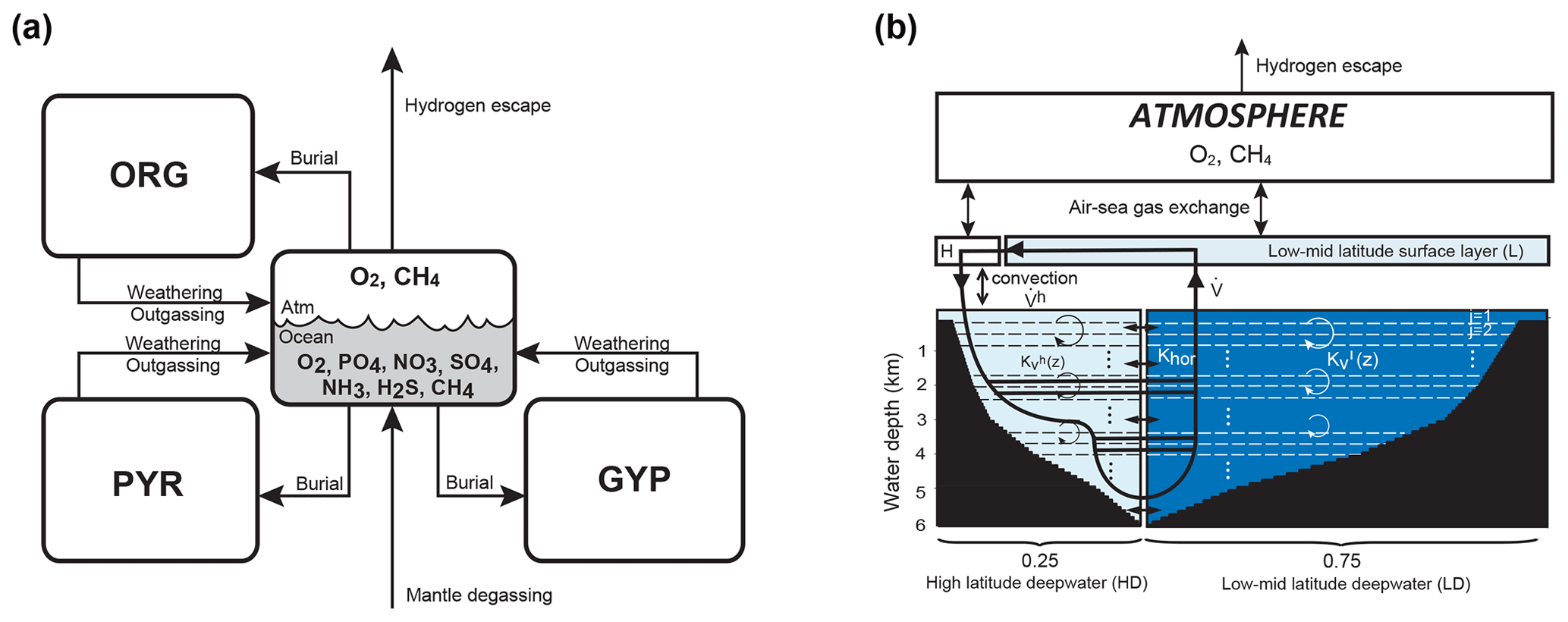
Figure 1 CANOPS-GRB model configuration.(a) The schematic of material cycles in the surface (ocean–atmosphere–crust) system. Three sedimentary reservoirs, organic carbon (ORG), pyrite sulfur (PYR), and gypsum sulfur (GYP), are considered. Sedimentary reservoirs interact with the ocean–atmosphere system via weathering, volcanic degassing, and burial. No interaction with the mantle is included, except for the input of reduced gases from the mantle. Total mass of sulfur is conserved in the surface system. (b) Schematic of ocean and atmosphere modules. “L” and “H” denote the low- to mid-latitude mixed surface layer and high-latitude surface layer, respectively. An ocean area of 10 % is assumed for H. River flux for each region is proportional to the areal fraction. Ocean interior is divided into two sectors, high-latitude deep water (HD) and low- to mid-latitude deep water (LD), which are vertically resolved. The area of HD is 25 % of the whole ocean. The deep overturning circulation, $\dot{V}$, equals the poleward flow in the model surface layer (from L to H). $K_{\mathrm{v}}^{\mathrm{l}}\left(z\right)$ and $K_{\mathrm{v}}^{\mathrm{h}}\left(z\right)$ are the vertical eddy diffusion coefficients in the LD and HD regions, respectively. K_hor and ${\dot{V}}_{\mathrm{h}}$ are the horizontal diffusion coefficient and polar convection, respectively. The black hatch represents the seafloor topography assumed. The parameters regarding geometry and water transport are tabulated in Table 3.

The ocean model is a vertically resolved transport reaction model of the global ocean, which was originally developed by Ozaki et al. (2011) and Ozaki and Tajika (2013). The model consists of 122 boxes across two regions – a low- to mid-latitude region and a high-latitude region (Fig. 1b). The ocean model describes water transport processes as exchange fluxes between boxes and via eddy diffusion terms. More specifically, ocean circulation is modeled as an advection–diffusion model of the global ocean – a general and robust scheme that is capable of producing well-resolved modern profiles of circulation tracers using realistic parameter values (the physical setup of the model can be found in Sect. 2.4.1 and 2.4.2). The biogeochemical sub-model provides a mechanistic description of the marine biogeochemical cycles of C, P, N, O₂, and S (Sect. 2.4.3). This includes explicit representation of a variety of biogeochemical processes such as biological productivity in the sunlit surface oceans; a series of respiration pathways and secondary redox reactions under oxic and anoxic conditions (Sect. 2.4.3); and deposition, decomposition, and burial of biogenic materials in marine sediments (Sect. 2.4.4), allowing a mechanistically based examination of biogeochemical processes. The suite of metabolic reactions included in the model is listed in Table 1. Ocean biogeochemical tracers considered in the CANOPS-GRB model are phosphate (PO${}_{\mathrm{4}}^{\mathrm{3}-}$), nitrate (NO${}_{\mathrm{3}}^{-}$), total ammonia (ΣNH₃), dissolved oxygen (O₂), sulfate (SO${}_{\mathrm{4}}^{\mathrm{2}-}$), total sulfide (ΣH₂S), and methane (CH₄). Note that biogeochemical cycling of trace metals (e.g., Fe and Mn) is not included in the current version of the model. All H₂S and NH₃ degassing from the ocean to the atmosphere is assumed to be completely oxidized by O₂ to SO${}_{\mathrm{4}}^{\mathrm{2}-}$ and NO${}_{\mathrm{3}}^{-}$ and returns to the ocean surface. These simplifications limit application of the model to very poorly oxygenated Earth system states (pO${}_{\mathrm{2}}<{\mathrm{10}}^{-\mathrm{5}}$ PAL). Ocean model performance was tested for the modern-day ocean field observational data (Sect. 3). Simulation results were also compared to previously published integrated global flux estimates.

The CANOPS model has been extended and altered a number of times since first publication. The description of biogeochemical cycles in the original version of CANOPS (Ozaki and Tajika, 2013; Ozaki et al., 2011) does not include the S and CH₄ cycles because of their aims to investigate the conditions for the development of oceanic anoxia and euxinia on timescales less than a million years during the Phanerozoic. More recently, Ozaki et al. (2019a) implemented an open-system modeling approach for the global S and CH₄ cycles, enabling quantitative analysis of global redox budget for given atmospheric O₂ levels and crustal reservoir sizes. In this version of CANOPS atmospheric O₂ levels and sedimentary reservoirs are treated as boundary conditions because imposing them simplifies the model and significantly reduces computing time. However, this approach does not allow exploration of the dynamic behavior of atmospheric O₂ in response to other boundary conditions. In the newest version presented here, significant improvements in the representation of global biogeochemistry were achieved by (1) an explicit calculation of atmospheric O₂ levels based on atmospheric mass balance (Sect. 2.6), (2) expansion of the model framework to include secular evolution of sedimentary reservoirs (Sect. 2.5.5), and (3) simplification of the global redox budget between the surface (ocean–atmosphere–crust) system and the mantle (Sect. 2.3.5). These improvements are in line with the requirement of an “open” Earth system model, which is necessary for a systematic, quantitative understanding of Earth's oxygenation history.

Table 1 Biogeochemical reactions considered in the CANOPS-GRB model.

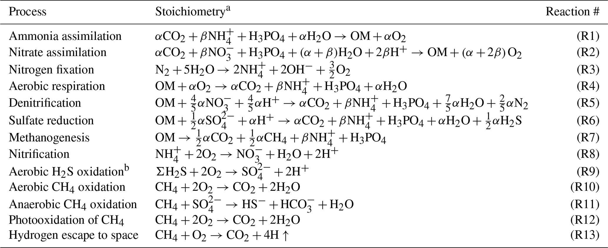
^a OM denotes organic matter, (CH₂O)_α(NH${}_{\mathrm{4}}^{+}{)}_{\mathit{\beta }}$H₃PO₄. ^b ΣH₂S = H₂S + HS⁻.

2.3 Global biogeochemical cycles

We construct a comprehensive biogeochemical model in order to investigate the interaction between dynamic behaviors of Earth's oxygenation history and its biogeochemical processes, as well as redox structure of the ocean. Here we provide the basic implementation of global biogeochemical cycles of C, P, N, and S, with particular emphasis on processes of mass exchange between reservoirs that play a critical role in global redox budget (Fig. 2). Our central aim here is to describe the overall design of the biogeochemical cycles. The details of each sub-model are provided in the following sections.

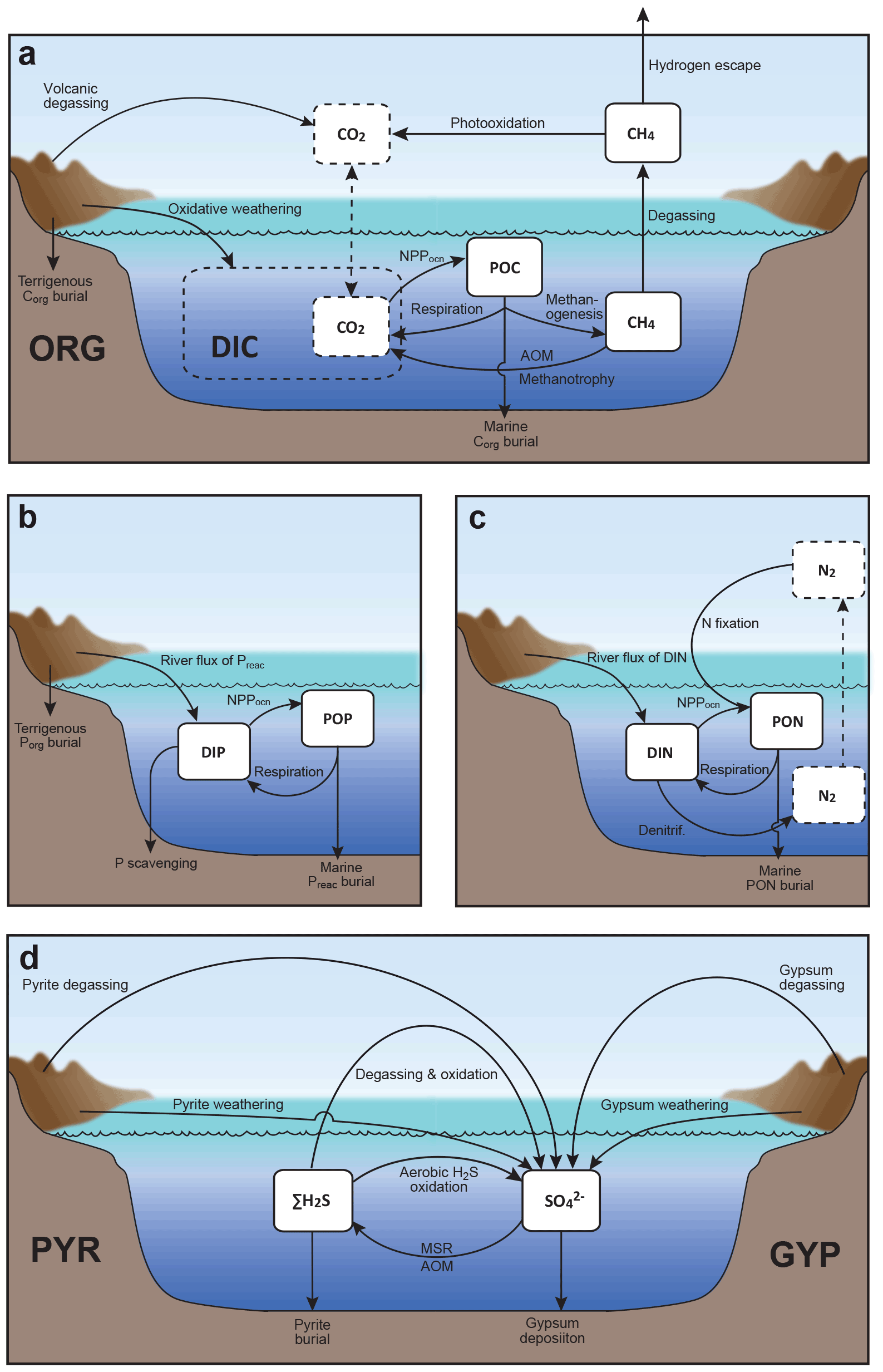
Figure 2 Schematics of global biogeochemical cycling in CANOPS-GRB. (a) Global C cycle. The primary source of C for the ocean–atmosphere system is volcanic degassing and oxidative weathering of sedimentary organic carbon, whereas primary sink is burial of marine and terrigenous organic matter into sediments. Inorganic carbon reservoirs (depicted as dashed boxes) and DOC are not considered. NPP_ocn represents marine net primary production. DIC stands for dissolved inorganic carbon. POC stands for particulate organic carbon. MSR stands for microbial sulfate reduction. AOM stands for anaerobic oxidation of methane. CANOPS-GRB includes CH₄ generation via methanogenesis and its oxidation reactions via methanotrophy and AOM in the ocean interior, as well as CH₄ degassing flux to the atmosphere and its photooxidation. The rates of CH₄ photooxidation and hydrogen escape to space are calculated based on parameterizations proposed by previous studies (Goldblatt et al., 2006; Claire et al., 2006). Note that CH₄ flux from land biosphere is not shown here. (b) Global P cycle schematic. Weathering of reactive P (P_reac) is the ultimate source, whereas burial in sediments is the primary sink. A part of the weathered P is buried as terrigenous organic P, and the remaining amount is delivered to the ocean. The redox-dependent P burial in marine sediments is modeled by considering three phases (organic P, Fe-bound P, and authigenic P). DIP stands for dissolved inorganic phosphorus. POP stands for particulate organic phosphorus. The hypothetical P scavenging via Fe species in anoxic-ferruginous waters is depicted, but it is not modeled in our standard model configuration. (c) Global N cycle schematic. The abundance of inorganic nitrogen species (ammonium and nitrate), which are lumped into DIN (dissolved inorganic nitrogen), is affected by denitrification and nitrification. The primary source is nitrogen fixation and riverine flux, whereas primary sink is denitrification and burial in marine sediments. PON stands for particulate organic nitrogen. The nitrogen weathering and riverine flux is assumed to be equal to the burial flux so that there is no mass imbalance in global N budget. Aeolian delivery of N from continent to the ocean is not included. (d) Global S cycle schematic. The reservoir sizes of sedimentary sulfur (pyrite sulfur, PYR, and gypsum sulfur, GYP) and two sulfur species (SO${}_{\mathrm{4}}^{\mathrm{2}-}$ and ΣH₂S) in the ocean are controlled by volcanic outgassing, weathering, burial, MSR, AOM, and sulfide oxidation reactions. Weathering and volcanic inputs are the primary source of S to the ocean, and burial of pyrite and gypsum in marine sediments is the primary sink. It is assumed that hydrogen sulfide escaping from the ocean to the atmosphere is completely oxidized and returns to the ocean as sulfate. The organic sulfur cycle is ignored in this study.

2.3.1 Carbon cycle

The CANOPS-GRB model includes particulate organic carbon (POC), atmospheric CH₄, dissolved CH₄ in the ocean, and sedimentary organic carbon (ORG) as carbon reservoirs (Fig. 2a). The primary sources of carbon for the ocean–atmosphere system are volcanic degassing and oxidative weathering of sedimentary organic carbon, while the primary sink is burial of marine and terrigenous organic matter in sediments. Atmospheric CO₂, dissolved inorganic carbon (DIC), and dissolved organic carbon (DOC) are not explicitly modeled in the current version of the model, and the full coupling of the inorganic carbon cycle within CANOPS-GRB is left as an important topic for future work. Neglecting the inorganic carbon cycle means that there are no climatic feedbacks in the system, and because of this simplification, the CANOPS-GRB model cannot be applied to problems such as those in which the Earth's climate and redox states of the ocean–atmosphere system are closely related each other or to validate model predictions based on geologic records (such as δ¹³C), but this allows us to avoid introducing additional complexities and uncertainties into the model.

Organic carbon cycle

The biogeochemical model is driven by the cycling of the primary nutrient phosphorus, which is assumed to be the ultimate limiting factor for biological productivity (see Sect. 2.4.3). Previous versions of CANOPS do not take into account the impact of the activity of terrestrial ecosystem on the global O₂ budget. In the CANOPS-GRB model, we improve on this by evaluating the activity levels of terrestrial and marine ecosystems separately. The global net primary production (NPP), J_NPP (in terms of organic C), is given as a sum of the oceanic ($J_{\mathrm{NPP}}^{\mathrm{ocn}}$) and terrestrial ($J_{\mathrm{NPP}}^{\mathrm{lnd}}$) NPP:

$$\begin{array}{}\text{(1)}& J_{\mathrm{NPP}}=J_{\mathrm{NPP}}^{\mathrm{ocn}}+J_{\mathrm{NPP}}^{\mathrm{lnd}}.\end{array}$$

Biological production in the ocean surface layer depends on P availability, while nutrient assimilation efficiency is assumed to be lower in the high-latitude region (Sect. 2.4.3). Terrestrial NPP is affected by the atmospheric O₂ level (Sect. 2.5.1). In this study, the flux (in terms of moles per year) is expressed with a capital J, whereas the flux density (in terms of moles per square meter per year) is expressed with a lowercase j.

In our standard model configuration, oceanic primary production follows canonical Redfield stoichiometry ($\mathrm{C}:\mathrm{N}:\mathrm{P}$ $=\mathrm{106}:\mathrm{16}:\mathrm{1}$) (Redfield et al., 1963). Flexible $\mathrm{C}:\mathrm{N}:\mathrm{P}$ stoichiometry of particulate organic matter (POM) can be explored by changing a user flag. Nutrients (P and N) are removed from seawater in the photic zone via biological uptake and exported as POM to deeper aphotic layers. The exported POM sinks through the water column with a speed of v_POM (the reference value is 100 m d⁻¹). As it settles through the water column, POM is subject to decomposition via a series of respiration pathways dependent on the redox state of proximal seawater (Sect. 2.4.3). This gives rise to the release of dissolved constituent species back into seawater. Within each layer a fraction of POM is also intercepted by a sediment layer at the bottom of each water depth. Fractional coverage of every ocean layer by seafloor is calculated based on the prescribed bathymetry (Sect. 2.4.1). Settling POM reaching the seafloor undergoes diagenetic alteration (releasing additional dissolved species into seawater) and/or permanent burial. The ocean model has 2×60 sediment segments (HD and LD have 60 layers, respectively), and for each segment the rates of organic matter decomposition and burial are calculated by semi-empirical relationships extracted from ocean sediment data and 1-D modeling of early diagenesis (Sect. 2.4.4). Specifically, the organic C (C_org) burial at each water depth is calculated based on the burial efficiency (BE_org), which is defined as the fraction of POC buried in sediments relative to that deposited on the seafloor at each water depth and is also a function of sedimentation rate and bottom-water O₂ levels. Organic matter not buried is subject to decomposition.

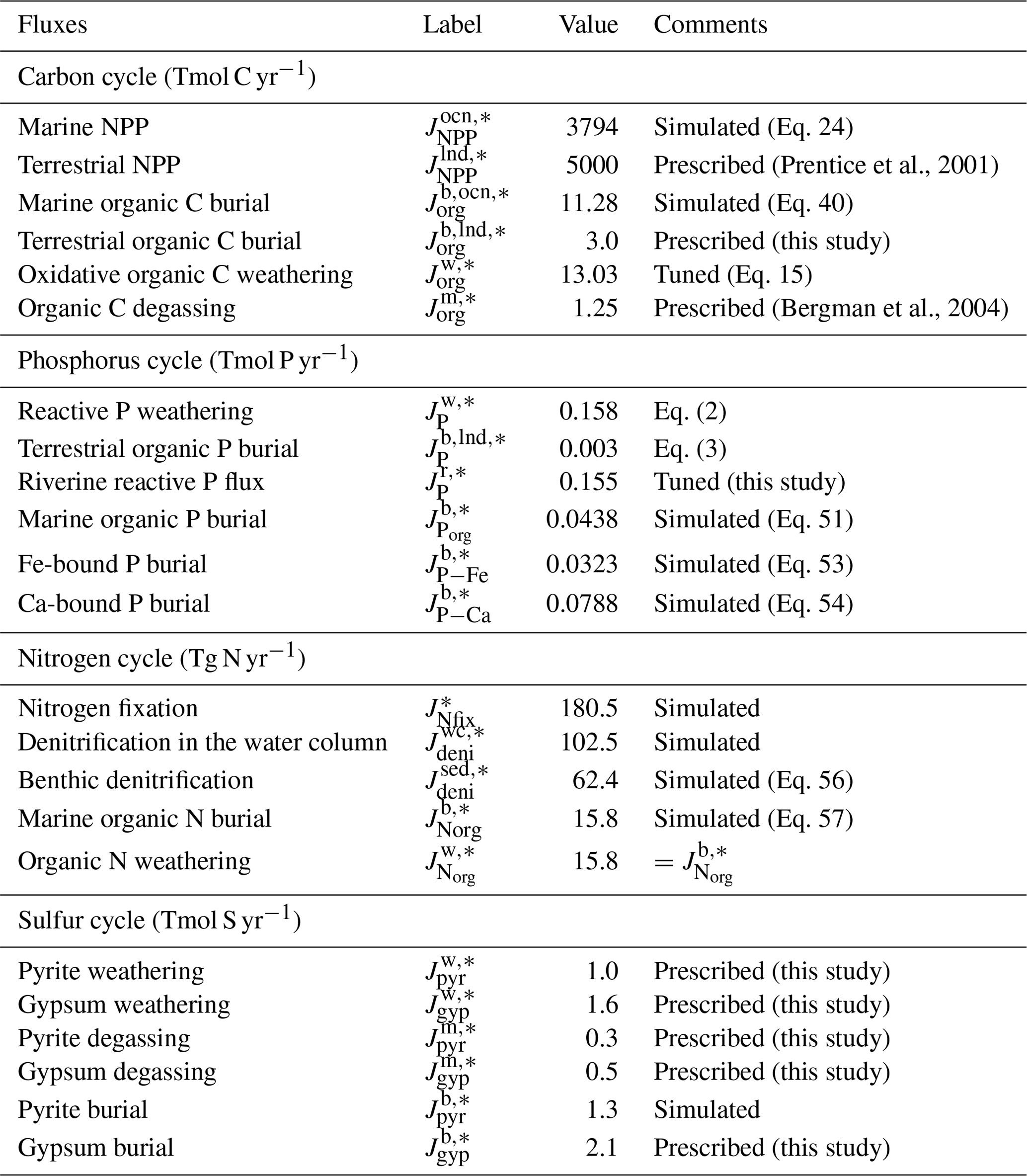
The key biogeochemical fluxes of our reference state (mimicking the present condition) are summarized in Table 2. The reference value for burial rate of terrigenous C_org is set at 3 Tmol C yr⁻¹, assuming that burial of terrigenous organic matter accounts for ∼20 % of the total burial. Combined with the burial rate of marine C_org in our standard run, the total burial rate is 14.3 Tmol C yr⁻¹, representing the dominant O₂ source flux to the modern ocean–atmosphere system. At steady state, this is balanced by oxidative weathering and volcanic outgassing of sedimentary C_org: The reference value of oxidative weathering of organic matter is determined as 13.0 Tmol C yr⁻¹ based on the global O₂ budget (Sect. 2.3.5). Previous versions of CANOPS (Ozaki et al., 2019a) treat sedimentary reservoirs as a boundary condition. This model limitation is removed in the CANOPS-GRB model – the reservoir size of sedimentary C_org (ORG) freely evolves based on the mass balance through burial, weathering, and volcanic outgassing (Sect. 2.5.5). We adopted an oft-quoted value of 1250 Emol (E=10¹⁸) for our reference value of the ORG, based on literature survey (Berner, 1989; Garrels and Lerman, 1981).

Table 2 Key biogeochemical fluxes obtained from the reference run. * denotes the reference value. Tmol = 10¹² mol, Tg = 10¹² g.

Methane cycle

The ocean model includes biogenic CH₄ generation via methanogenesis and its oxidation reactions via methanotrophy and anaerobic oxidation of methane (AOM) in the ocean interior (Reactions R10 and R11 in Table 1), as well as a CH₄ degassing flux to the atmosphere. The land model also calculates the biogenic CH₄ flux from the terrestrial ecosystem to the atmosphere using a transfer function (Sect. 2.5.2). The abundance of CH₄ in the atmosphere is explicitly modeled as a balance of its source (degassing from marine and terrestrial ecosystems) and sink (photooxidation and hydrogen escape), where CH₄ sink fluxes are calculated according to parameterized O₂-dependent functions proposed by previous studies. More specifically, the oxidation rate of CH₄ in the upper atmosphere is calculated based on the empirical parameterization obtained from a 1-D photochemistry model (Claire et al., 2006). The rate of hydrogen escape to space is evaluated with the assumption that it is diffusion limited and that CH₄ is a major H-containing chemical compound carrying hydrogen to the upper atmosphere (Goldblatt et al., 2006). No continental abiotic or thermogenic CH₄ fluxes are taken into account because previous estimates of the modern fluxes are negligible relative to the biogenic flux, although we realize that it could have played a role in the global redox budget (<0.3 Tmol yr⁻¹; Fiebig et al., 2009). We also note that the current version of the model does not include the possibility of aerobic CH₄ production in the sea (Karl et al., 2008). Our reference run calculates atmospheric CH₄ to be 0.16 ppmv (Fig. 17), slightly lower than that of the preindustrial level of 0.7 ppmv (Raynaud et al., 1993; Etheridge et al., 1998), but we consider this to be within reasonable error given unknowns in the CH₄ cycle.

2.3.2 Phosphorus cycle

Phosphorus is an essential element for all life on Earth and it is regarded as the “ultimate” bio-limiting nutrient for primary productivity on geologic timescales (Tyrrell, 1999). Thus, the P cycle plays a prominent role in regulating global O₂ levels. In the CANOPS-GRB model, we model the reactive (i.e., bioavailable) P (P_reac) cycling in the system and ignore non-bioavailable P. Specifically, dissolved inorganic P (DIP) and particulate organic P (POP) are explicitly modeled (Fig. 2b), whereas dissolved organic P (DOP) is ignored.

On geologic timescales, the primary source of P to the ocean–atmosphere system is continental weathering: a phosphorus is released through the dissolution of apatite which exists as a trace mineral in silicate and carbonate rocks (∼0.1 wt %; Föllmi, 1996). The total P_reac flux via weathering, $J_{\mathrm{P}}^{\mathrm{w}}$, is given as follows:

$$\begin{array}{}\text{(2)}& J_{\mathrm{P}}^{\mathrm{w}}=f_{\mathrm{P}}{f}_{\mathrm{R}}{J}_{\mathrm{P}}^{\mathrm{w},\ast },\end{array}$$

where * denotes the reference value and f_P and f_R are parameters that control the availability of P in the system. Specifically, f_R is a global erosion factor representing the impact of tectonic activity on total terrestrial weathering rate, and f_P represents the availability of P_reac, which is used in a sensitivity experiment to assess the response of atmospheric O₂ levels to changing P_reac availability (Sect. 4.1). A fraction of the weathering flux $J_{\mathrm{P}}^{\mathrm{w}}$ is removed via burial on land, while the remainder is transported to the ocean:

$$\begin{array}{}\text{(3)}& {\displaystyle }{J}_{\mathrm{P}}^{\mathrm{b},\mathrm{lnd}}=k_{\mathrm{11}}V{J}_{\mathrm{P}}^{\mathrm{w}},\text{(4)}& {\displaystyle }{J}_{\mathrm{P}}^{\mathrm{r}}=(\mathrm{1}-k_{\mathrm{11}}V)J_{\mathrm{P}}^{\mathrm{w}},\end{array}$$

where $J_{\mathrm{P}}^{\mathrm{b},\mathrm{lnd}}$ and $J_{\mathrm{P}}^{\mathrm{r}}$ denote the burial rate of terrigenous organic P and riverine P_reac flux to the ocean, respectively, k₁₁ is a reference value for the fraction of the total P flux removed by the terrestrial biosphere, and V denotes the vegetation mass normalized to the modern value. These treatments are based on the Earth system box model COPSE (Bergman et al., 2004; Lenton et al., 2016, 2018; Lenton and Watson, 2000b), which has been extensively tested and validated against geologic records during the Phanerozoic. In the CANOPS-GRB model, $J_{\mathrm{P}}^{\mathrm{r}}$ is tuned so that modeled oceanic P inventory of the reference state is consistent with modern observations of the global ocean (Sect. 3.2.3). Our resulting tuned value is 0.155 Tmol P yr⁻¹, falling in the mid-range of published estimates of 0.11–0.33 Tmol P yr⁻¹, although previous estimates of the riverine P_reac flux show large uncertainty (Sect. 3.2.3).

Note that our representation of P weathering ignores the effect of climate (Eq. 2). In the current version of the model the rate of P weathering is treated as one of the model forcings. Although ignoring the climate feedback on P mobility makes interpretation of the model results more straightforward, the incorporation of a climate-sensitive crustal P cycle is an important avenue for future work.

Since atmospheric P inputs are equivalent to less than 10 % of the continental P supply to the modern oceans and much of this flux is not bioavailable (Graham and Duce, 1979), we neglect the aeolian flux in this study. Therefore, riverine input is the primary source of P_reac to the ocean. We highlight that open-system modeling is crucial for realistic simulations of ocean biogeochemistry on timescales longer than the residence time of P in the ocean (15–20 kyr for the modern ocean) (Hotinski et al., 2000), and in this framework the riverine input of P_reac must be balanced over the long term by loss to sediments via burial. The change in total marine P_reac inventory, M_P, is given as follows:

$$\begin{array}{}\text{(5)}& {\displaystyle \frac{\mathrm{d}{M}_{\mathrm{P}}}{\mathrm{d}t}}=J_{\mathrm{P}}^{\mathrm{r}}-J_{\mathrm{P}}^{\mathrm{b},\mathrm{ocn}},\end{array}$$

where $J_{\mathrm{P}}^{\mathrm{b},\mathrm{ocn}}$ denotes the total burial flux of P_reac in the marine system, which is the sum of the burial fluxes of three reactive phases, i.e., organic P (P_org), Fe-bound P (P-Fe), and Ca-bound P (P-Ca) (Sect. 2.4.4):

$$\begin{array}{}\text{(6)}& J_{\mathrm{P}}^{\mathrm{b},\mathrm{ocn}}=J_{\mathrm{Porg}}^{\mathrm{b}}+J_{\mathrm{P}-\mathrm{Fe}}^{\mathrm{b}}+J_{\mathrm{P}-\mathrm{Ca}}^{\mathrm{b}}.\end{array}$$

O₂-dependent P burial is taken into account using empirical relationships from previous studies (Slomp and Van Cappellen, 2007; Van Cappellen and Ingall, 1996, 1994). The burial of P_org at each water depth is a function of burial efficiency, which is controlled by the burial efficiency of organic matter, $\mathrm{C}/\mathrm{P}$ stoichiometry of POM, sedimentation rate, and bottom-water [O₂]. We note that the strength of anoxia-induced P recycling in marine sediments is very poorly constrained, especially in the Precambrian oceans (Reinhard et al., 2017b). Recent studies also suggest that the P retention potential in marine sediments could be affected not only by bottom-water O₂ levels but also by redox states (sulfidic vs. ferruginous) and the Ca²⁺ concentration of bottom waters, as well as various environmental conditions such as temperature and pH (Zhao et al., 2020; Algeo and Ingall, 2007; Papadomanolaki et al., 2022). These are fruitful topics for future research.

We do not explicitly account for P removal via hydrothermal processes because it is estimated that this contribution is secondary in the modern marine P cycle (0.014–0.036 Tmol P yr⁻¹; Wheat et al., 1996, 2003). We note, however, that the hydrothermal contribution to the total P budget in the geologic past remains poorly constrained. We also note that in anoxic, ferruginous oceans, P scavenging by Fe minerals could also play an important role in controlling P availability and the overall budget (Reinhard et al., 2017b; Derry, 2015; Laakso and Schrag, 2014). Modern observations (Dellwig et al., 2010; Turnewitsch and Pohl, 2010; Shaffer, 1986) and modeling efforts (Yakushev et al., 2007) of the redoxcline in the Baltic Sea and the Black Sea suggest an intimate relationship between Mn, Fe, and P cycling. Trapping efficiencies of DIP by settling authigenic Fe and Mn-rich particles were found to be as high as 0.63 (the trapping efficiency is defined as the downward flux of P in Mn and Fe oxides divided by the upward flux of DIP) (Turnewitsch and Pohl, 2010). Although coupled Mn–Fe–P dynamics might have been a key aspect of the biogeochemical dynamics in the Precambrian oceans, we exclude this process in our standard model due to poor constraints and provide a clear and simplified picture of basic model behavior. The key features between the P availability and atmospheric O₂ levels are explored by changing f_P in this study (Sect. 4).

2.3.3 Nitrogen cycle

In the CANOPS-GRB model, two dissolved inorganic nitrogen (DIN) species (total ammonium ΣNH${}_{\mathrm{4}}^{+}$ and nitrate NO${}_{\mathrm{3}}^{-}$) and particulate organic nitrogen (PON) are explicitly calculated (Fig. 2c). Atmospheric nitrogen gas is assumed to never limit biospheric carbon fixation and is not explicitly calculated. Dissolved organic N (DON) and terrestrial N cycling (e.g., N fixation by terrestrial ecosystems and riverine-terrigenous organic N transfer) are ignored.

In the surface ocean, N assimilation via nitrate and ammonium depends on the availability of these compounds. If the N required for sustaining a given level of biological productivity is not available, the additional N required is assumed to be provided by atmospheric N₂ via nitrogen fixers. The ocean model explicitly calculates denitrification and nitrification reactions in the water column and marine sediments (Reactions R5 and R8 in Table 1). The benthic denitrification rate is estimated using a semi-empirical parameterized function obtained from a 1-D early diagenetic model (see Sect. 2.4.4), while nitrification is modeled as a single step reaction (Reaction R8). N₂O and its related reactions, such as anammox, are not currently included.

The oceanic N cycle is open to external inputs of nitrogen. While the ultimate source of N to the ocean–atmosphere system is weathering of organic N, nitrogen fixation represents the major input flux to the ocean with the capacity to compensate for N loss due to denitrification. The time evolution of DIN inventory, M_N, in the ocean can be written as follows:

$$\begin{array}{}\text{(7)}& {\displaystyle \frac{\mathrm{d}{M}_{\mathrm{N}}}{\mathrm{d}t}}=\left(J_{{\mathrm{N}}_{\mathrm{fix}}}-J_{\mathrm{deni}}^{\mathrm{wc}}-J_{\mathrm{deni}}^{\mathrm{sed}}\right)+\left(J_{{\mathrm{N}}_{\mathrm{org}}}^{\mathrm{w}}-J_{\mathrm{Norg}}^{\mathrm{b}}\right),\end{array}$$

where $J_{{\mathrm{N}}_{\mathrm{fix}}}$ denotes the N fixation rate and $J_{\mathrm{deni}}^{\mathrm{wc}}$ and $J_{\mathrm{deni}}^{\mathrm{sed}}$ are denitrification rates in the water column and sediments, respectively. The first set of terms on the right-hand side represents the internal N cycle in the ocean–atmosphere system, while the second set of terms represents the long-term N budget which interacts with sedimentary reservoir. Ultimately, loss of fixed N from the ocean–atmosphere system only occurs via burial of organic N (N_org) in sediments, $J_{{\mathrm{N}}_{\mathrm{org}}}^{\mathrm{b}}$. This loss is compensated for by continental weathering, $J_{{\mathrm{N}}_{\mathrm{org}}}^{\mathrm{w}}$, which is assumed to be equal to the burial rate of N_org so that the N cycle has no impact on the global redox budget. In the current version of the model, we ignore aeolian flux and all riverine N fluxes other than weathering since these are minor relative to N fixation (Wang et al., 2019). As a result, modeled N fixation required for oceanic N balance can be regarded as an upper estimate.

2.3.4 Sulfur cycle

The original CANOPS ocean model (Ozaki and Tajika, 2013; Ozaki et al., 2011) treated two sulfur species, SO${}_{\mathrm{4}}^{\mathrm{2}-}$ and ΣH₂S, in a closed system. Neither inputs to the ocean from rivers, hydrothermal vents, and submarine volcanoes nor outputs due to evaporite formation and sedimentary pyrite burial were simulated. This simplification can be justified when the timescale of interest is less than the residence time of the S cycle (∼10–20 Myr). The recently revised CANOPS model (Ozaki et al., 2019a) extends the framework by incorporating the S budget in the ocean. In their model framework, the sedimentary S reservoirs are treated as boundary conditions. The size of sedimentary gypsum and pyrite reservoirs are prescribed, and no explicit calculations of mass balance are performed. In CANOPS-GRB, we removed this model limitation, and the sedimentary reservoirs are explicitly evaluated based on mass balance which is controlled by burial, outgassing and weathering (see Sect. 2.5.5). Specifically, seawater SO${}_{\mathrm{4}}^{\mathrm{2}}$, ΣH₂S, and sedimentary sulfur reservoirs of pyrite sulfur (PYR) and gypsum sulfur (GYP) are explicitly evaluated in the current version of the model. No atmospheric sulfur species are calculated – all H₂S degassing from the ocean to the atmosphere is assumed to be oxidized to sulfate and to return to the ocean. The organic sulfur cycle is not considered in this study.

Sulfur enters the ocean mainly from river runoff, $J_{\mathrm{S}}^{\mathrm{r}}$, with minor contributions from volcanic outgassing of sedimentary pyrite, $J_{\mathrm{pyr}}^{\mathrm{m}}$, and gypsum, $J_{\mathrm{gyp}}^{\mathrm{m}}$. The reference value for the riverine flux is set at 2.6 Tmol S yr⁻¹, consistent with the published estimate of 2.6±0.6 Tmol S yr⁻¹ (Raiswell and Canfield, 2012). The riverine flux is written as the sum of gypsum weathering and oxidative weathering of pyrite: $J_{\mathrm{S}}^{\mathrm{r}}=J_{\mathrm{gyp}}^{\mathrm{w}}+J_{\mathrm{pyr}}^{\mathrm{w}}$. Sulfur weathering fluxes are also assumed to be proportional to the sedimentary reservoir size. Estimates of modern volcanic input fall within the range of 0.3–3 Tmol S yr⁻¹ (Catling and Kasting, 2017; Kagoshima et al., 2015; Raiswell and Canfield, 2012; Walker and Brimblecombe, 1985). We adopted a value of 0.8 Tmol S yr⁻¹ for this flux (Kagoshima et al., 2015). Our total input of 3.4 Tmol S yr⁻¹ is also within the range of the previous estimate of 3.3±0.7 Tmol S yr⁻¹ (Raiswell and Canfield, 2012). Sulfur is removed from the ocean either via pyrite burial, $J_{\mathrm{pyr}}^{\mathrm{b}}$, or gypsum deposition, $J_{\mathrm{gyp}}^{\mathrm{b}}$ (Fig. 2d). The time evolution of the inventory of total S in the ocean can thus be written as follows:

$$\begin{array}{}\text{(8)}& {\displaystyle \frac{\mathrm{d}\left(M_{{\mathrm{SO}}_{\mathrm{4}}}+M_{{\mathrm{H}}_{\mathrm{2}}\mathrm{S}}\right)}{\mathrm{d}t}}=\left(J_{\mathrm{S}}^{\mathrm{r}}+J_{\mathrm{pyr}}^{\mathrm{m}}+J_{\mathrm{gyp}}^{\mathrm{m}}\right)-\left(J_{\mathrm{pyr}}^{\mathrm{b}}+J_{\mathrm{gyp}}^{\mathrm{b}}\right),\end{array}$$

where $M_{{\mathrm{SO}}_{\mathrm{4}}}$ and $M_{{\mathrm{H}}_{\mathrm{2}}\mathrm{S}}$ denote the inventory of sulfate and hydrogen sulfide in the ocean, respectively. Two sulfur species (SO${}_{\mathrm{4}}^{\mathrm{2}-}$ and ΣH₂S) are transformed via microbial sulfate reduction (MSR) (Reaction R6), AOM (Reaction R11), and aerobic sulfide oxidation reactions (Reaction R9). The above equation thus can be divided into following equations:

$$\begin{array}{}\text{(9)}& {\displaystyle \frac{\mathrm{d}{M}_{{\mathrm{SO}}_{\mathrm{4}}}}{\mathrm{d}t}}=J_{\mathrm{S}}^{\mathrm{r}}+J_{\mathrm{pyr}}^{\mathrm{m}}+J_{\mathrm{gyp}}^{\mathrm{m}}+J_{{\mathrm{H}}_{\mathrm{2}}\mathrm{S}}^{\mathrm{ox}}-J_{\mathrm{MSR}\mathrm{\&}\mathrm{AOM}}-J_{\mathrm{gyp}}^{\mathrm{b}},\text{(10)}& {\displaystyle \frac{\mathrm{d}{M}_{{\mathrm{H}}_{\mathrm{2}}\mathrm{S}}}{\mathrm{d}t}}=-J_{{\mathrm{H}}_{\mathrm{2}}\mathrm{S}}^{\mathrm{ox}}+J_{\mathrm{MSR}\mathrm{\&}\mathrm{AOM}}-J_{\mathrm{pyr}}^{\mathrm{b}},\end{array}$$

where $J_{{\mathrm{H}}_{\mathrm{2}}\mathrm{S}}^{\mathrm{ox}}$ denotes the oxidation of hydrogen sulfide and J_MSR&AOM is sulfate reduction via MSR and AOM. Pyrite burial is represented as the sum of pyrite precipitation in the water column and sediments: $J_{\mathrm{pyr}}^{\mathrm{b}}=J_{\mathrm{pyr}}^{\mathrm{b},\mathrm{wc}}+J_{\mathrm{pyr}}^{\mathrm{b},\mathrm{sed}}$, where the pyrite burial rate in marine sediments is assumed to be proportional to the rate of benthic sulfide production. The proportional coefficient, pyrite burial efficiency (e_pyr), is one of the tunable constants of the model. For normal (oxic) marine sediments, e_pyr is tuned such that the seawater SO${}_{\mathrm{4}}^{\mathrm{2}-}$ concentration for our reference run is consistent with modern observations (Sect. 2.4.4). Pyrite precipitation in the water column is assumed to be proportional to the concentration of ΣH₂S.

Although the present-day marine S budget is likely out of balance because of a lack of major gypsum formation, the S cycle can be considered to operate at steady state on timescales longer than the residence time of sulfur in the ocean. According to S isotope mass balance calculations, ∼10 %–45 % of the removal flux is accounted for by pyrite burial, and the remainder is removed via formation of gypsum and anhydrite in the near-modern oceans (Tostevin et al., 2014). Although gypsum deposition would have been strongly influenced by tectonic activity (Halevy et al., 2012), we assume that the rate of gypsum deposition on geologic timescales is proportional to the ion product of Ca²⁺ and SO${}_{\mathrm{4}}^{\mathrm{2}-}$ (Berner, 2004b) in the low- to mid-latitude surface layer (L) and is defined as follows:

$$\begin{array}{}\text{(11)}& J_{\mathrm{gyp}}^{\mathrm{b}}=\left({\displaystyle \frac{\left[{\mathrm{Ca}}^{\mathrm{2}+}{]}_{\mathrm{l}}\right[{\mathrm{SO}}_{\mathrm{4}}^{\mathrm{2}-}{]}_{\mathrm{l}}}{\left[{\mathrm{Ca}}^{\mathrm{2}+}{]}^{\ast }\right[{\mathrm{SO}}_{\mathrm{4}}^{\mathrm{2}-}{]}^{\ast }}}\right)J_{\mathrm{gyp}}^{\mathrm{b},\ast }=f_{\mathrm{Ca}}\left({\displaystyle \frac{[{\mathrm{SO}}_{\mathrm{4}}^{\mathrm{2}-}{]}_{\mathrm{l}}}{[{\mathrm{SO}}_{\mathrm{4}}^{\mathrm{2}-}{]}^{\ast }}}\right)J_{\mathrm{gyp}}^{\mathrm{b},\ast },\end{array}$$

where “l” denotes the low- to mid-latitude surface layer and f_Ca is a parameter that represents the seawater Ca²⁺ concentration normalized by the present value (f_Ca=1 for the reference run). The reference value of gypsum burial $J_{\mathrm{gyp}}^{\mathrm{b},\ast }$ is determined by assuming that gypsum deposition accounts for ∼60 % of the total S removal from the near-modern ocean.

2.3.5 Global redox budget

In the previous version of the CANOPS model (Ozaki et al., 2019a), the atmospheric O₂ level was prescribed as a boundary condition, rather than modeled in order to limit computational demands. In this study, we remove this model limitation by introducing an explicit mass balance calculation of atmospheric O₂ (Sect. 2.6.3). This improvement allows us to explore the dynamic response of O₂ levels in the ocean-atmosphere system (Sect. 4).

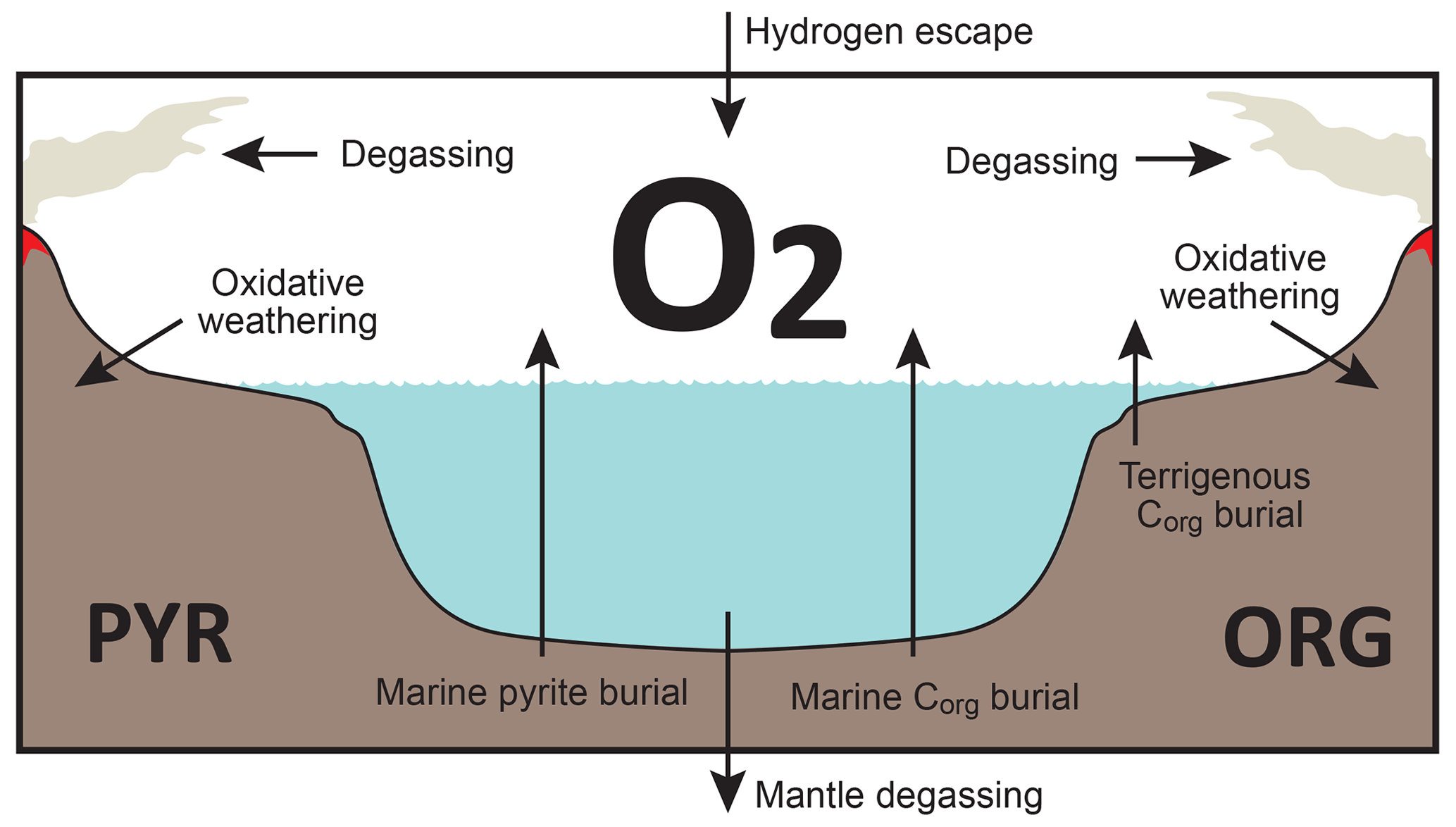
Figure 3 Schematics of global redox (O₂) budget. Arrows represent the O₂ flux. The primary source is burial of organic carbon and pyrite sulfur in sediments and hydrogen escape to space. The primary sink is volcanic outgassing and weathering of crustal organic matter and pyrite. PYR is the sedimentary reservoir of pyrite sulfur. ORG is the sedimentary reservoir of organic carbon. CANOPS-GRB tracks the global redox (O₂) budget for each simulation.

CANOPS-GRB v1.0 is designed to be a part of a comprehensive global redox budget (GRB) framework (Fig. 3) (Catling and Kasting, 2017; Ozaki and Reinhard, 2021). Here GRB is defined for the combined ocean–atmosphere system. In this study we track GRB in terms of O₂ equivalents. The ultimate source of O₂ is the activity of oxygenic photosynthesis (and subsequent burial of reduced species, such as organic matter and pyrite sulfur, in sediments), whereas the primary sink of O₂ is the oxidative weathering of organic carbon and pyrite which are assumed to be O₂ dependent (Sect. 2.5.3). On timescales longer than the residence time of O₂ in the ocean–atmosphere system, O₂ source fluxes should be balanced by sink fluxes. Specifically, the O₂ budget in the coupled ocean–atmosphere system can be expressed as follows:

$$\begin{array}{}\text{(12)}& \begin{array}{rl}\mathrm{GRB}& =\left(J_{\mathrm{org}}^{\mathrm{b},\mathrm{ocn}}+J_{\mathrm{org}}^{\mathrm{b},\mathrm{lnd}}-J_{\mathrm{org}}^{\mathrm{w}}-J_{\mathrm{org}}^{\mathrm{m}}\right)\\ & +\mathrm{2}\left(J_{\mathrm{pyr}}^{\mathrm{b}}-J_{\mathrm{pyr}}^{\mathrm{w}}-J_{\mathrm{pyr}}^{\mathrm{m}}\right)+\left(J_{\mathrm{Hesc}}-J_{\mathrm{man}}\right),\end{array}\end{array}$$

where the first and second set of terms on the right-hand side represent the redox balance via organic carbon and pyrite sulfur subcycles, respectively. J_Hesc in the third term denotes hydrogen escape to space, representing the irreversible oxidation of the system. For well-oxygenated atmospheres this process plays a minor role in the redox budget, but for less-oxygenated atmospheres with high levels of CH₄ this flux could lead to redox imbalance. In this study we include the input of reducing power (e.g., H₂ and CO) from the Earth's interior to the surface, J_man, which is assumed to be equal to the value of J_Hesc (J_man=J_Hesc) to avoid redox imbalance in the exogenic system. In reality, mantle degassing and the rate of hydrogen escape are not necessarily equal, resulting in redox imbalance that may exert a fundamental control on atmospheric redox chemistry on geologic timescales (Hayes and Waldbauer, 2006; Ozaki and Reinhard, 2021; Canfield, 2004; Eguchi et al., 2020); however, to maintain simplicity we have left this as a topic for future work. As a result, the terms on the right-hand side must be balanced at steady state. Our model can meet this criterion. Note that the effects of the Fe cycle on the O₂ budget (e.g., the oxidative weathering of Fe(II)-bearing minerals; Ozaki et al., 2019a) are not included in the core version of the CANOPS-GRB v1.0 code and in the analyses presented here for the sake of simplicity.

The CANOPS-GRB model also tracks the O₂ budgets for the atmosphere (ARB) and ocean (ORB) independently:

$$\begin{array}{}\text{(13)}& {\displaystyle }\begin{array}{rl}\text{ARB}& ={\mathrm{\Phi }}_{\mathrm{ex}}^{\mathrm{air}-\mathrm{sea}}+\left(J_{\mathrm{org}}^{\mathrm{b},\mathrm{lnd}}-J_{\mathrm{org}}^{\mathrm{w}}-J_{\mathrm{org}}^{\mathrm{m}}\right)\\ & -\mathrm{2}\left(J_{\mathrm{pyr}}^{\mathrm{w}}+J_{\mathrm{pyr}}^{\mathrm{m}}\right)+\left(J_{\mathrm{Hesc}}-J_{\mathrm{man}}\right),\end{array}\text{(14)}& {\displaystyle }\text{ORB}=-{\mathrm{\Phi }}_{\mathrm{ex}}^{\mathrm{air}-\mathrm{sea}}+J_{\mathrm{org}}^{\mathrm{b},\mathrm{ocn}}+\mathrm{2}{J}_{\mathrm{pyr}}^{\mathrm{b}},\end{array}$$

where ${\mathrm{\Phi }}_{\mathrm{ex}}^{\mathrm{air}-\mathrm{sea}}$ represents the net exchange of oxidizing power between the ocean and atmosphere via gas exchange (O₂ with minor contributions of NH₃, H₂S and CH₄). These separate redox budgets are also tracked in order to validate global budget calculations.

For our reference condition, we obtain the reference value for the oxidative weathering rate of C_org ($J_{\mathrm{org}}^{\mathrm{w},\ast }$) using the redox budget via C_org subcycle:

$$\begin{array}{}\text{(15)}& J_{\mathrm{org}}^{\mathrm{w},\ast }=J_{\mathrm{org}}^{\mathrm{b},\mathrm{ocn},\ast }+J_{\mathrm{org}}^{\mathrm{b},\mathrm{lnd},\ast }-J_{\mathrm{org}}^{\mathrm{m},\ast }.\end{array}$$

Given flux values based on the calculated ($J_{\mathrm{org}}^{\mathrm{b},\mathrm{ocn},\ast }=\mathrm{11.28}$ Tmol C yr⁻¹) and prescribed ($J_{\mathrm{org}}^{\mathrm{b},\mathrm{lnd},\ast }=\mathrm{3}$ Tmol C yr⁻¹, $J_{\mathrm{org}}^{\mathrm{m},\ast }=\mathrm{1.25}$ Tmol C yr⁻¹) values on the right-hand side, $J_{\mathrm{org}}^{\mathrm{w},\ast }$ is estimated as 13.03 Tmol C yr⁻¹ (Table 2).

2.4 Ocean model

Here we undertake a thorough review, reconsideration, and revision (where warranted) of all aspects of the ocean model, including bringing together developments of the model following the original papers describing the CANOPS ocean model framework (Ozaki and Tajika, 2013; Ozaki et al., 2011).

The ocean model includes exchange of chemical species with external systems via several processes such as air–sea exchange, riverine input, and sediment burial. The biogeochemical model also includes a series of biogeochemical processes, such as the ocean biological pump and redox reactions under oxic, anoxic, and sulfidic conditions. Our ocean model is convenient for investigating Earth system changes on timescales of hundreds of years or longer and can be relatively easily integrated, rendering the model unique in terms of biogeochemical cycle models. CANOPS is also well suited for sensitivity studies and can be used to obtain useful information upstream of more complex models.

Development of the ocean model included two initial goals: First, to adopt a general and robust ocean circulation scheme capable of producing well-resolved modern distributions of circulation tracers using realistic ventilation rates with a limited number of free parameters. The model outputs for circulation tracers are validated by comparison with modern observations (see Sect. 3). This confirms that our ocean circulation scheme is adequate for representing the global patterns of water mass transport. A second key goal was to couple the circulation model with an ocean biogeochemical model and to evaluate performance by comparison with modern ocean biogeochemical data (see Sect. 3.2). Examination of the distributions and globally integrated fluxes of C, N, P, S, and O₂ for the modern ocean reveals that the ocean model can capture the fundamentals of marine biogeochemical cycling.

2.4.1 Structure

CANOPS ocean model is a 1-D (vertically resolved) intermediate-complexity box model of ocean biogeochemistry (see Fig. 1b for the schematic structure) originally developed by Ozaki and Tajika (2013) and Ozaki et al. (2011). Our model structure is an improved version of the HILDA model (Joos et al., 1991; Shaffer and Sarmiento, 1995). Unlike simple one-dimensional global ocean models (e.g., Southam et al., 1982), the HILDA-type model includes explicit high-latitude dynamics whereby the high-latitude surface layer exchanges properties with the deep ocean. This treatment is crucial for simulating preformed properties and observed chemical distributions, especially for phosphate and dissolved O₂ in a self-consistent manner. Unlike simple box-type global ocean models, the model has high vertical resolution. This is needed for representing proper biogeochemical processes that show strong depth dependency. Furthermore, HILDA type models (Arndt et al., 2011; Shaffer et al., 2008), unlike multi-box-type global ocean models (Hotinski et al., 2000), use a small number of free parameters to represent ocean physics and biology. The simple and adaptable structure of the model should make it applicable to a wide range of paleoceanographic problems. The ocean model couples a diffusion-advection model of the global ocean surface and interior with a biogeochemical model (Sect. 2.4.3) and a parameterized sediment model (Sect. 2.4.4).

The ocean surface consists of a mixed layer at low- to mid-latitude (L) and high-latitude (H). Below the surface layers, we adopt the present-day averaged seafloor topography of Millero (2006), with the hypsometric profile shown in Fig. 4a. Below the surface water layers, the ocean interior comprises two regions: the high- to mid-latitude region (HD) and the low- to mid-latitude region (LD). Each region is subdivided vertically with high resolution (Δz=100 m). Each of the 60 ocean layers in each latitude region (120 total) is assigned ocean sediment properties. The cross-sectional area, volume, and sediment surface area of each box is calculated from the benthic hypsometry. Inclusion of the bathymetry allows evaluation of the flux of biogenic materials which settle on, and are buried in, seafloor sediments at each water depth (Sect. 2.4.3 and 2.4.4).

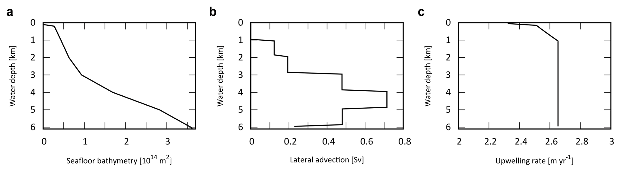
Figure 4 Ocean bathymetry and water transport. (a) Seafloor topography (cumulative seafloor area) (Millero, 2006) adopted in the CANOS-GRB model. (b) Lateral water advection from HD to LD section assumed in the standard run (in Sv). Total advection rate $\dot{V}$ was set at 20 Sv. (c) Upwelling rate in the LD region (in m yr⁻¹) of the standard run.

2.4.2 Transport

The ocean circulation model represents a general and robust scheme that is capable of producing well-resolved modern profiles of circulation tracers using realistic parameter values and the coupled biogeochemical model (Sect. 2.4.3) or parameterized sediment model (Sect. 2.4.4).

The time–space evolution of model variables in the ocean is described by a system of horizontally integrated vertical diffusion equations for non-conservative substances. The tracer conservation equation establishes the relationship between change of tracer concentration at a given grid point and the processes that can change that concentration. These processes include water transport by advection and mixing and sources and sinks due to biological and chemical transformations. The temporal and spatial evolution of the concentration of a dissolved component in the aphotic zone is described by a horizontally integrated vertical diffusion equation, which relates the rate of change of tracer concentration at a given point to the processes that act to change the tracer concentration:

$$\begin{array}{}\text{(16)}& {\displaystyle \frac{\partial \left[X\right]}{\partial t}}={\left.{\displaystyle \frac{\partial \left[X\right]}{\partial t}}\right|}_{\mathrm{trans}}+{\mathrm{\Theta }}_{\mathrm{bio}}+{\mathrm{\Theta }}_{\mathrm{react}},\end{array}$$

where [X] represents horizontally integrated physical variables (such as potential temperature, salinity, or ¹⁴C) or concentration of a chemical component, t denotes time, and Θ_bio and Θ_react represent internal sources and sinks associated with the biological pump and chemical reactions, respectively. An external source or sink term Θ_ex, which represents riverine input and/or air–sea gas exchange, is added to the surface layers. The first term on the right-hand side of Eq. (16) represents the physical transport:

$$\begin{array}{}\text{(17)}& \begin{array}{rl}{\left.{\displaystyle \frac{\partial \left[X\right]}{\partial t}}\right|}_{\mathrm{trans}}& =-A^{\mathrm{l},\mathrm{h}}\left(z\right)w^{\mathrm{l},\mathrm{h}}\left(z\right){\displaystyle \frac{\partial \left[X\right]}{\partial z}}\\ & +{\displaystyle \frac{\partial }{\partial z}}\left(A^{\mathrm{l},\mathrm{h}}\left(z\right)K_{\mathrm{v}}^{\mathrm{l},\mathrm{h}}\left(z\right){\displaystyle \frac{\partial \left[X\right]}{\partial z}}\right)+K_{\mathrm{hor}}{\displaystyle \frac{{\partial }^{\mathrm{2}}\left[X\right]}{\partial y^{\mathrm{2}}}}.\end{array}\end{array}$$

The terms on the right-hand side express (from left to right) the advection, vertical diffusion, and horizontal diffusion. Here, l and h indicate the LD and HD, respectively. The factors $K_{\mathrm{v}}^{\mathrm{l},\mathrm{h}}(z$), K_hor, A^l,h(z), and w^l,h(z) denote the vertical and horizontal diffusion coefficients, the areal fraction of the water layer at water depth z to the sea surface area, and upwelling (for LD) or downwelling (for HD) velocity, respectively.

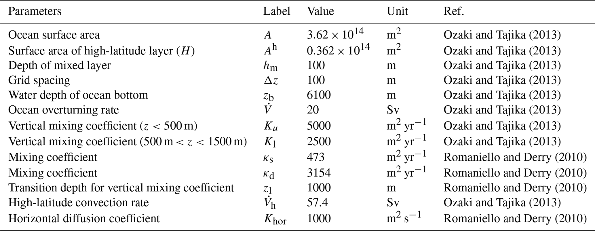
In the CANOPS ocean model, ocean circulation and mixing are characterized by five physical parameters: (1) water transport via thermohaline circulation, $\dot{V}$, associated with high-latitude sinking and low- to mid-latitude upwelling, (2) constant horizontal diffusion between the aphotic zones, K_hor, (3) strong, depth-dependent vertical diffusion between the aphotic zones in the high-latitude region, $K_{\mathrm{v}}^{\mathrm{h}}(z$), (4) high-latitude convection, ${\dot{V}}_{\mathrm{h}}$, and (5) depth-dependent vertical diffusion in the low- to mid-latitude region, $K_{\mathrm{v}}^{\mathrm{l}}(z$). These parameters are tuned to give tracer distributions consistent with present-day observations. Thermohaline circulation and high-latitude convection are considered to be general physical modes on any rotating planet, and our simplified water transport scheme allows us to represent them with a limited number of free parameters. However, we emphasize that the water transport scheme explored here is designed to represent the modern ocean circulation on Earth. As a result, some of these parameterizations may need to be modified when being applied to ancient oceans or oceans on exoplanets. Nevertheless, given our simple design, our water transport scheme is relatively flexible to modify the water circulations that are markedly different from the modern ocean.

Advection

Advective water transport in the ocean model represents the major features of modern meridional overturning circulation. The rate of production of ventilated ocean waters ranges from 14 to 27 Sv (1 Sv = 10⁶ m³ s⁻¹) in the North Atlantic and from 18 to 30 Sv in the Southern Ocean (e.g., Doney et al., 2004; Lumpkin and Speer, 2007). The formation of deepwater effectively supplies “fresh” ventilated water to the abyss. We choose $\dot{V}=\mathrm{20}$ Sv as a reference value, giving a mean overturning time of about 2140 years, consistent with the ventilation time estimated from observations (Broecker and Peng, 1982).

The downwelling of the surface waters at H forms HD that flows into the intermediate to deep oceanic layers of LD, which in turn upwells over L (Fig. 1b). In many one-dimensional ocean models, downwelling water enters the ocean interior via the deepest model layer (e.g., Southam et al., 1982; Shaffer and Sarmiento, 1995; Volk and Hoffert, 1985). In the real ocean, downwelling waters are transported along isopycnal layers below approximately 1000 m (e.g., Doney et al., 2004; Lumpkin and Speer, 2007; Shaffer and Sarmiento, 1995; Volk and Hoffert, 1985). Hence, we assume that high-latitude deep water flows into each ocean layer below 1100 m. While there is some uncertainty in the pattern of lateral advection, the flow is determined in our model assuming a constant upwelling rate below a depth of 1100 m in the LD region. The upwelling and downwelling rate w^l,h(z) is then determined by the seafloor topography and the deep-water lateral inflow, assuming continuity. Figure 4b shows the lateral advection of deep waters with a reference circulation rate $\dot{V}$ of 20 Sv. This assumption provides a plausible upwelling rate, which is consistent with the oft-quoted value of 2–3 m yr⁻¹ (Broecker and Peng, 1982) (Fig. 4c).

Vertical mixing

Ocean circulation is dominated by turbulent processes driven by wind and tidal mixing. These processes occur as eddies, which occur at a wide range of spatial scales, from centimeters to whole ocean basins. In numerical models of ocean circulation, turbulent mixing in the ocean interior is commonly represented as a diffusion process, characterized by an eddy diffusion coefficient. The vertical eddy diffusion coefficient K_v(z) is typically on the order of 10⁻⁵ to 10⁻⁴ m² s⁻¹, and it is common to assume a depth dependence that smoothly increases from the thermocline ($\sim {\mathrm{10}}^{-\mathrm{5}}$ m² s⁻¹) to the abyss ($\sim {\mathrm{10}}^{-\mathrm{4}}$ m² s⁻¹) using an inverse or hyperbolic tangent function (e.g., Shaffer et al., 2008; Yakushev et al., 2007). To account for thermocline ventilation, we assumed a relatively high vertical diffusion coefficient in mid-water depth ($K_{\mathrm{l}}=\mathrm{6.3}\times {\mathrm{10}}^{-\mathrm{5}}$ m² s⁻¹ for water depth 500–1500 m). We also adopted a higher value for the vertical diffusion coefficient ($K_u=\mathrm{1.6}\times {\mathrm{10}}^{-\mathrm{4}}$ m² s⁻¹) in the uppermost 500 m of the ocean in order to represent the highly convective Ekman layer in the upper part of the ocean.

$$\begin{array}{}\text{(18)}& K_{\mathrm{v}}^{\mathrm{l}}\left(z\right)=\left\{\begin{array}{l}{K}_{\mathrm{u}}(z\ge -\mathrm{500}\mathrm{m})\\ K_{\mathrm{l}}(-\mathrm{500}\ge z\ge -\mathrm{1500}\mathrm{m})\\ {\mathit{\kappa }}^{\mathrm{s}}+\frac{{\mathit{\kappa }}^{\mathrm{d}}-{\mathit{\kappa }}^{\mathrm{s}}}{\mathrm{2}}\left(\mathrm{1}+\tanh \left(\frac{z-z^{\mathrm{l}}}{z^{\mathrm{l}}}\right)\right)\left(\text{otherwise}\right)\end{array}\right.,\end{array}$$

where κ^s and κ^d are vertical mixing coefficients and z^l is the transition length scale (Romaniello and Derry, 2010). In the high-latitude region where no permanent thermocline exists, more rapid communication with deep waters can occur. Previous studies have pointed out that the vertical diffusivities at high latitude can be very high (up to O(10⁻² m² s⁻¹)) (e.g., Sloyan, 2005). To account for this we include high-latitude convection between H and YD (${\dot{V}}_{\mathrm{h}}=\mathrm{57.4}$ Sv) and higher vertical diffusion ($K_{\mathrm{v}}^{\mathrm{h}}\left(z\right)=\mathrm{2}\times K_{\mathrm{v}}^{\mathrm{l}}\left(z\right)$).

Horizontal diffusion

The horizontal diffusivity is included according to Romaniello and Derry (2010). On basin scales, the horizontal (isopycnal) eddy diffusivity is 10⁷–10⁸ times larger than the vertical (diapycnal) eddy diffusivity due to anisotropy of the density field. For a spatial scale of 1000 km, horizontal eddy diffusion is estimated to be O(10³ m² s⁻¹) (e.g., Ledwell et al., 1998). We adopt this value. As Romaniello and Derry (2010) did previously, we assume horizontal mixing follows the pathways of advective fluxes between laterally adjacent regions. The reciprocal exchange fluxes may be written as

$$\begin{array}{}\text{(19)}& J_{\mathrm{hor}}^{\mathrm{ex}}=K_{\mathrm{hor}}{A}_{\perp }{\displaystyle \frac{\partial \left[X\right]}{\partial y}}={\displaystyle \frac{K_{\mathrm{hor}}{A}_{\perp }}{L}}\mathrm{\Delta }\left[X\right],\end{array}$$

where $J_{\mathrm{hor}}^{\mathrm{ex}}$ denotes the exchange fluxes between the layers (in mol yr⁻¹), A_⊥ represents the cross-sectional area separating two adjacent reservoirs, L is a characteristic spatial distance separating the reservoirs, and Δ[X] is the difference in concentration between two reservoirs (Romaniello and Derry, 2010). By assuming that L is of the same order as the length of the interface separating the two regions, we can approximate $A_{\perp }\approx \mathrm{\Delta }z\times O(L$), where Δz is the thickness of the interface separating the two regions. Then we obtain

$$\begin{array}{}\text{(20)}& J_{\mathrm{hor}}^{\mathrm{ex}}=K_{\mathrm{hor}}\mathrm{\Delta }z\mathrm{\Delta }\left[X\right].\end{array}$$

Therefore, when we discretize the ocean interior at 100 m spacing approximately 0.1 Sv of reciprocal mixing occurs between adjacent layers.

Ocean circulation tracers

We use potential temperature θ, salinity S, and radioactive carbon ¹⁴C, as physical tracers. Distributions of these tracers are determined by the transport mechanisms described above. In this study, we adopt the values at the surface layers (L and H) as upper boundary conditions: θ^l=15 ^∘C, θ^h=0 ^∘C, S^l=35 psu, S^h=34 psu, Δ¹⁴C${}^{\mathrm{l}}=-\mathrm{40}$ ‰, and Δ¹⁴C${}^{\mathrm{h}}=-\mathrm{100}$ ‰. The radioactive decay rate for ¹⁴C is $\mathrm{1.21}\times {\mathrm{10}}^{-\mathrm{4}}$ yr⁻¹. Although ¹⁴C can be incorporated in the biogenic materials and transported into deep water, we ignore this biological effect for simplicity. The associated error is ∼10 % of the profiles produced by circulation and radioactive decay (Shaffer and Sarmiento, 1995). The parameter values used in the ocean circulation model are listed in Table 3.

Table 3 Physical setup of the ocean circulation model.

2.4.3 Ocean biogeochemical framework

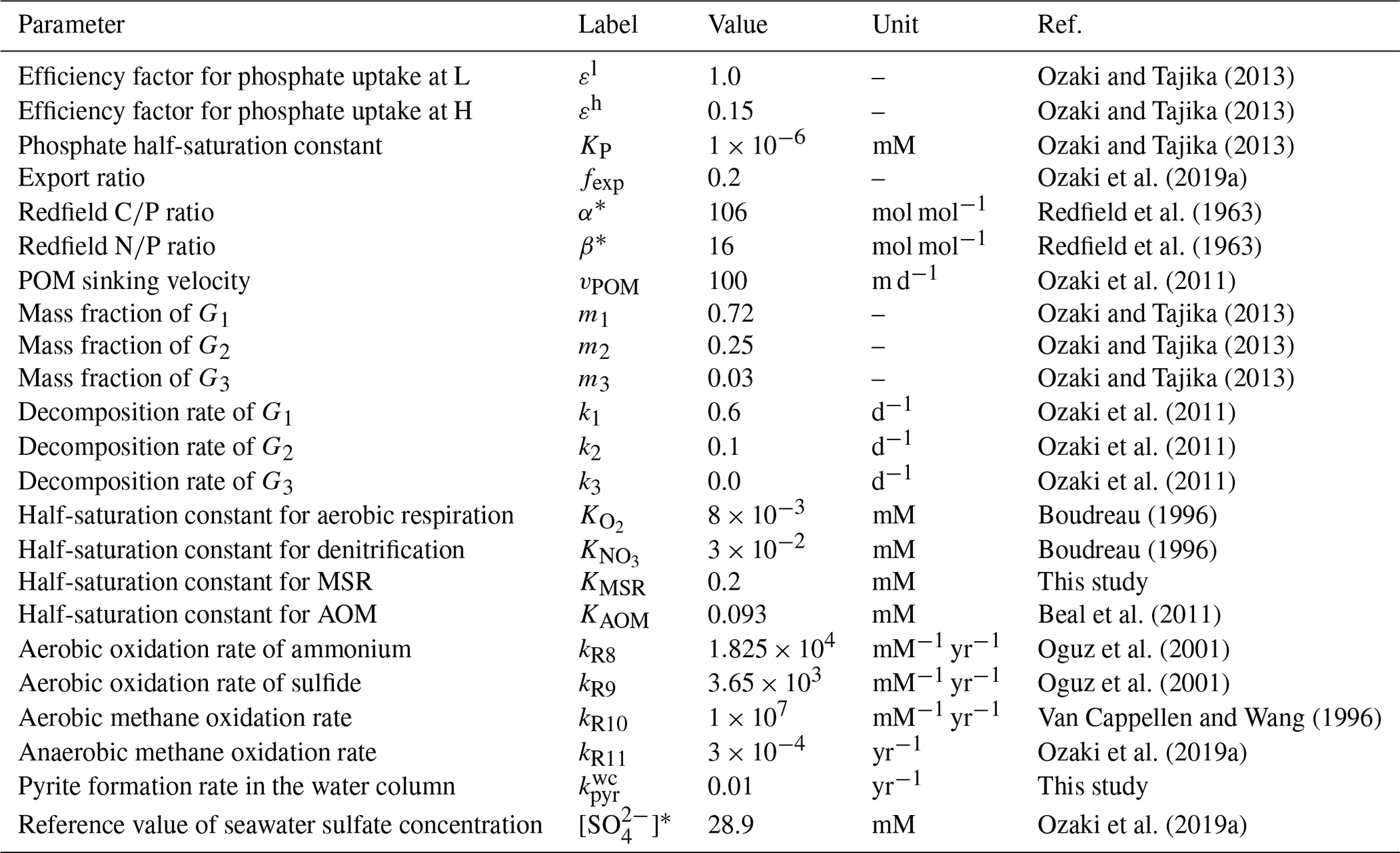
The ocean circulation model is coupled to a biogeochemical model, which includes an explicit representation of a variety of biogeochemical processes in the ocean. The parameters used in the oceanic biogeochemical model are listed in Table 4.

Table 4 Parameter values used in the oceanic biogeochemistry module of CANOPS-GRB.

Biological production

The overall biogeochemical cycling scheme is based on the cycling of primary nutrient (phosphate; PO${}_{\mathrm{4}}^{\mathrm{3}-}$), which limits biological productivity – export production is related to the availability of P within the euphotic zone (Maier-Reimer, 1993; Yamanaka and Tajika, 1996; Shaffer et al., 2008):

$$\begin{array}{}\text{(21)}& j_{\exp }^{\mathrm{l},\mathrm{h}}={\mathit{\alpha }}^{\mathrm{l},\mathrm{h}}{h}_{\mathrm{m}}{\mathit{\epsilon }}^{\mathrm{l},\mathrm{h}}[{\mathrm{PO}}_{\mathrm{4}}^{\mathrm{3}-}{]}^{\mathrm{l},\mathrm{h}}{\displaystyle \frac{[{\mathrm{PO}}_{\mathrm{4}}^{\mathrm{3}-}{]}^{\mathrm{l},\mathrm{h}}}{[{\mathrm{PO}}_{\mathrm{4}}^{\mathrm{3}-}{]}^{\mathrm{l},\mathrm{h}}+K_{\mathrm{P}}}},\end{array}$$

where j_exp represents new and export production of POC (in unit of mol C m⁻² yr⁻¹), α denotes C:P stoichiometry of POM, h_m is the mixed-layer depth, ε denotes the assimilation efficiency factor for P uptake, and K_P denotes the half-saturation constant. The value of ε for the low- to mid-latitude region is assumed to be 1. In contrast, we assume a lower efficiency for the high-latitude region because biological production tends to be limited by environmental factors other than phosphate availability (e.g., amount of solar radiation, mixed-layer thickness, sea ice formation, and iron availability). This is used as one of the fitting parameters in the model. Downwelling waters contain a certain level of nutrients (i.e., preformed nutrients).

In our standard run, the stoichiometry of organic matter is parameterized using the canonical Redfield ratio ($\mathrm{C}:\mathrm{N}:\mathrm{P}$ = $\mathrm{106}:\mathrm{16}:\mathrm{1}$) (Redfield et al., 1963). However, we note that flexible $\mathrm{C}:\mathrm{N}:\mathrm{P}$ stoichiometry has been the subject of recent discussion. In the modern oceans, $\mathrm{C}:\mathrm{N}:\mathrm{P}$ ratios of exported POM vary across latitude, reflecting ecosystem structure (Galbraith and Martiny, 2015). Local observations (and laboratory experiments) suggest that the $\mathrm{C}:\mathrm{N}:\mathrm{P}$ ratio of cyanobacteria is a function of seawater PO${}_{\mathrm{4}}^{\mathrm{3}-}$ concentration (Larsson et al., 2001). The evolutionary perspective has also been discussed (Quigg et al., 2003; Sharoni and Halevy, 2022). In the previous version of the CANOPS model, the C–N–P stoichiometry of primary producers responds dynamically to P availability in the surface layer (Reinhard et al., 2017b):

$$\begin{array}{}\text{(22)}& {\displaystyle }\mathit{\alpha }={\mathit{\alpha }}^{\ast }+{\displaystyle \frac{{\mathit{\alpha }}_{\max }-{\mathit{\alpha }}^{\ast }}{\mathrm{2}}}\left(\mathrm{1}+\tanh \left({\displaystyle \frac{{\mathit{\gamma }}_{\mathrm{P}\mathrm{0}}-\left[{\mathrm{PO}}_{\mathrm{4}}^{\mathrm{3}-}\right]}{{\mathit{\gamma }}_{\mathrm{P}\mathrm{1}}}}\right)\right),\text{(23)}& {\displaystyle }\mathit{\beta }={\mathit{\beta }}^{\ast }+{\displaystyle \frac{{\mathit{\beta }}_{\max }-{\mathit{\beta }}^{\ast }}{\mathrm{2}}}\left(\mathrm{1}+\tanh \left({\displaystyle \frac{{\mathit{\gamma }}_{\mathrm{P}\mathrm{0}}-\left[{\mathrm{PO}}_{\mathrm{4}}^{\mathrm{3}-}\right]}{{\mathit{\gamma }}_{\mathrm{P}\mathrm{1}}}}\right)\right),\end{array}$$

where α and β represent the $\mathrm{C}/\mathrm{P}$ ratio and $\mathrm{N}/\mathrm{P}$ ratio of POM, * denotes the canonical Redfield ratios, max denotes the maximum value (α_max=400 and β_max=60), and γ_P0 and γ_P1 are tunable constants (γ_P0=0.1 µM and γ_P1=0.03 µM) (Kuznetsov et al., 2008). In the CANOPS-GRB model, this dynamic response of POM stoichiometry can be explored by changing the user flag from the standard static response. In this study, we do not explore the impacts of flexible POM stoichiometry on global biogeochemistry (i.e., ${\mathit{\alpha }}_{\max }={\mathit{\alpha }}^{\ast }$ and ${\mathit{\beta }}_{\max }={\mathit{\beta }}^{\ast }$).

Biological production in the surface mixed layer increases the concentration of dissolved O₂ and reduces the concentrations of DIP and DIN according to the stoichiometric ratio (Reactions R1 and R2; Table 1). DIN consumption is partitioned between nitrate and ammonium, assuming that ammonium is preferentially assimilated. CANOPS-GRB evaluates the availability of fixed N in the surface ocean, and any N deficiency required for a given level of productivity is assumed to be compensated for on geologic timescales by N fixers. In other words, it is assumed that biological N fixation keeps pace with P availability so that P (not N) ultimately determines oceanic biological productivity.

To date, models of varying orders of complexity have been developed to simulate oceanic primary production and nutrient cycling in the euphotic layer, from a single nutrient and single phytoplankton component system to the inclusion of multiple nutrients and trophic levels in the marine ecosystem, usually coupled to physical models (e.g., Yakushev et al., 2007; Oguz et al., 2000). To avoid this level of complexity, we introduce a parameter, f_exp, called export ratio (Sarmiento and Gruber, 2006), which relates the flux densities of export production and NPP, as follows:

$$\begin{array}{}\text{(24)}& j_{\mathrm{NPP}}^{\mathrm{ocn}}={\displaystyle \frac{j_{\exp }}{f_{\exp }}},\end{array}$$

where $j_{\mathrm{NPP}}^{\mathrm{ocn}}$ denotes the NPP in terms of mol C m⁻² yr⁻¹. In the modern ocean, the globally averaged value of f_exp is estimated at 0.2 (Laws et al., 2000), and we assumed this value in this study. The rate of recycling of organic matter in the photic zone is thus given by

$$\begin{array}{}\text{(25)}& j_{\mathrm{recy}}=j_{\mathrm{NPP}}^{\mathrm{ocn}}-j_{\exp }={\displaystyle \frac{\mathrm{1}-f_{\exp }}{f_{\exp }}}{j}_{\exp }.\end{array}$$

The respiration pathway of j_recy depends on the availability of terminal electron acceptors (O₂, NO${}_{\mathrm{3}}^{-}$ and SO${}_{\mathrm{4}}^{\mathrm{2}-}$). Following exhaustion of these species as terminal electron acceptors, organic matter remineralization occurs by methanogenesis (Reaction R7). See below for the treatment of organic matter remineralization in the water column.

Biological pump

Most POM exported to the deep sea is remineralized in the water column before reaching the seafloor (e.g., Broecker and Peng, 1982). Nutrients returning to seawater at intermediate depths may rapidly return to the surface ocean and support productivity. The remaining fraction of POM that reaches the sediment ultimately exerts an important control on oceanic inventories of nutrients and O₂. An adequate representation of the strength of biological pump is therefore critical to any descriptions of global biogeochemical cycles.

The governing equation of the concentration of biogenic particles G is

$$\begin{array}{}\text{(26)}& {\displaystyle \frac{\partial G}{\partial t}}+v_{\mathrm{POM}}{\displaystyle \frac{\partial G}{\partial z}}=-rG,\end{array}$$

where r is a decomposition rate and v_POM is the settling velocity of POM in the water column. We assume a settling velocity of 100 m d⁻¹ for our reference value (e.g., Suess, 1980), although a very wide range of values and depth dependencies have been reported (e.g., Berelson, 2001a). Therefore, the settling velocity is fast enough to neglect advective and diffusive transport of biogenic particles. Note that the settling velocity would affect the intensity of biological pump and chemical distribution in the ocean interior. Considering the ballast hypothesis in the modern ocean (Armstrong et al., 2001; Francois et al., 2002; Ittekkot, 1993; Klaas and Archer, 2002), the settling velocity of POM in the geological past would very likely have been different from the modern ocean. As Kashiyama et al. (2011) pointed out, there would be a critical aspect among sinking rate of POM, intensity of biological pump and chemical distribution in the ocean. The quantitative and comprehensive evaluation of their effect is an important issue for the future work (Fakhraee et al., 2020).

In order to solve Eq. (26) explicitly, a relatively small time step (∼1 d) would be required. However, because the sinking velocity and remineralization of biogenic material are fast processes, we assume that the POM export and remineralization occurs in the same time step (ignoring the term $\partial G/\partial t$). The concentration of biogenic particles can be solved as follows:

$$\begin{array}{}\text{(27)}& G(z+\mathrm{\Delta }z)=G\left(z\right)\exp \left(-{\displaystyle \frac{r\mathrm{\Delta }z}{v_{\mathrm{POM}}}}\right),\end{array}$$

where Δz is a spatial resolution of the model.

Organic matter decomposition

As POM settles through the water column, it is nearly entirely decomposed back to dissolved tracers. Therefore, decomposition of POM is a key process for modeling biogeochemistry in the ocean. To avoid the complex treatment of this process (such as repackaging and aggregation or dispersal of particles), various empirical schemes for POM sinking flux have been proposed, such as exponential (Volk and Hoffert, 1985) or power law (Martin et al., 1987) functions (Fig. 5). However, the estimation of Volk and Hoffert generally tends to overestimate in the upper water column (<1.5 km) and underestimate at depth. It is important to note that data series of sediment trap measurements were obtained from a limited geographic and depth range. Berelson (2001b) and Lutz et al. (2002) conducted further estimates of the sediment flux and found regional variability in the sinking flux. Broadly, these data indicate that commonly applied flux relationships generally tend to overestimate flux to depth.

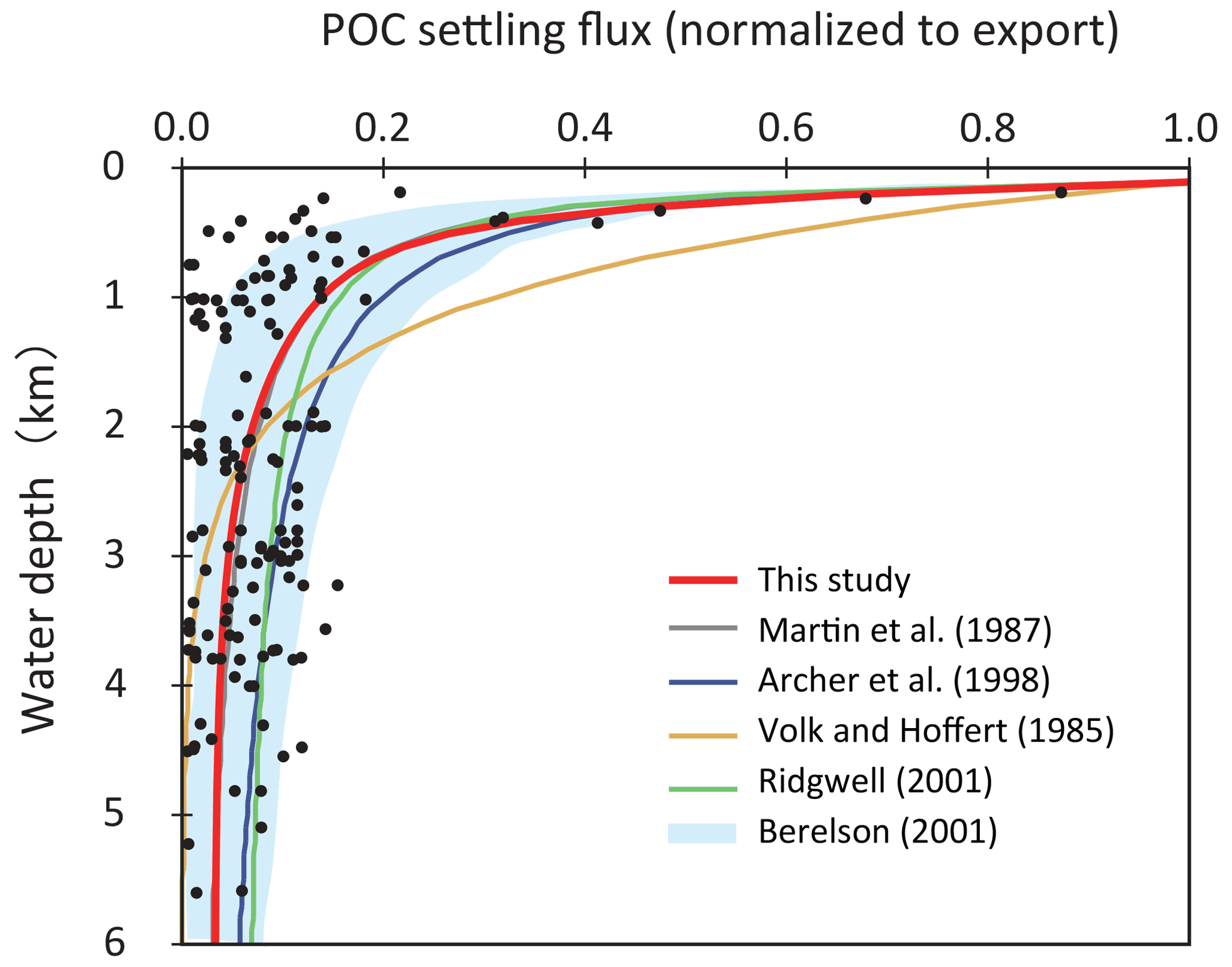
Figure 5 Empirical relationships between POC settling flux normalized to export production (Lutz et al., 2002) and water depth (Archer et al., 1998; Berelson, 2001b; Martin et al., 1987; Volk and Hoffert, 1985). The profile of the CANOPS-GRB model is depicted as a red line. The black dots represent observational data (Honjo and Manganini, 1993; Lutz et al., 2002; Tsunogai and Noriki, 1991; Honjo, 1980, and references therein).

The microbial degradation of different groups of organic matter differs over timescales ranging from hours to millions of years. In order to represent the decrease in POM lability with time and water depth, we adopt the so-called multi-G model (Westrich and Berner, 1984) that describes the detailed kinetics of organic matter decomposition (Ozaki and Tajika, 2013; Ozaki et al., 2011). In the CANOPS model, POM is described using two degradable fractions (G₁ and G₂) and one inert (G₃) fraction using different rate constants k_i (i=1, 2, 3) for each component. Rate constants are tuned on the basis of consistency with the typical profile of the POM sinking flux estimated from sediment trap studies (Fig. 5). In this study, constant stoichiometries between C, N, and P during the remineralization of POM are assumed throughout the water column, taking values equal to those characterizing mean export production.

The electron acceptor used in the respiration reaction changes from dissolved O₂ to other oxidants (e.g., NO${}_{\mathrm{3}}^{-}$ and SO${}_{\mathrm{4}}^{\mathrm{2}-}$) as O₂ becomes depleted. The respiration pathway is controlled by the free energy change per mole of organic carbon oxidized. The organic matter decomposition is performed by the oxidant that yields the greatest free energy change per mole of organic carbon oxidized. When the oxidant is depleted, further decomposition will proceed utilizing the next most efficient (i.e., the most energy producing) oxidant until either all oxidants are consumed or oxidizable organic matter is depleted (e.g., Froelich et al., 1979; Berner, 1989). In oxic waters, organic matter is remineralized by an aerobic oxidation process (Reaction R4). As dissolved O₂ is depleted, NO${}_{\mathrm{3}}^{-}$ and/or SO${}_{\mathrm{4}}^{\mathrm{2}-}$ will be used (Reactions R5 and R6). Denitrification is carried out by heterotrophic bacteria under low concentrations of dissolved O₂ if there is sufficient nitrate. For anoxic, sulfate-lean oceans, the methanogenic degradation of organic matter will occur (Reaction R7). In the CANOPS-GRB model, we parameterized the dependence of decomposition of POM with a Michaelis–Menten type relationship with respect to the terminal electron acceptors:

$$\begin{array}{}\text{(28)}& {\displaystyle }{R}_{\mathrm{4}}={\displaystyle \frac{\left[{\mathrm{O}}_{\mathrm{2}}\right]}{K_{{\mathrm{O}}_{\mathrm{2}}}+\left[{\mathrm{O}}_{\mathrm{2}}\right]}}\left(\sum k_i{G}_i\right)\text{(29)}& {\displaystyle }{R}_{\mathrm{5}}={\displaystyle \frac{K_{{\mathrm{O}}_{\mathrm{2}}}^{\prime }}{K_{{\mathrm{O}}_{\mathrm{2}}}^{\prime }+\left[{\mathrm{O}}_{\mathrm{2}}\right]}}{\displaystyle \frac{\left[{\mathrm{NO}}_{\mathrm{3}}^{-}\right]}{K_{{\mathrm{NO}}_{\mathrm{3}}}+\left[{\mathrm{NO}}_{\mathrm{3}}^{-}\right]}}\left(\sum k_i{G}_i\right),\text{(30)}& {\displaystyle }\begin{array}{rl}{R}_{\mathrm{6}}& ={\displaystyle \frac{K_{{\mathrm{O}}_{\mathrm{2}}}^{\prime }}{K_{{\mathrm{O}}_{\mathrm{2}}}^{\prime }+\left[{\mathrm{O}}_{\mathrm{2}}\right]}}{\displaystyle \frac{K_{{\mathrm{NO}}_{\mathrm{3}}}^{\prime }}{K_{{\mathrm{NO}}_{\mathrm{3}}}^{\prime }+\left[{\mathrm{NO}}_{\mathrm{3}}^{-}\right]}}\\ & \cdot {\displaystyle \frac{\left[{\mathrm{SO}}_{\mathrm{4}}^{\mathrm{2}-}\right]}{K_{\mathrm{MSR}}+\left[{\mathrm{SO}}_{\mathrm{4}}^{\mathrm{2}-}\right]}}\left(\sum k_i{G}_i\right),\end{array}\text{(31)}& {\displaystyle }\begin{array}{rl}{R}_{\mathrm{7}}& ={\displaystyle \frac{K_{{\mathrm{O}}_{\mathrm{2}}}^{\prime }}{K_{{\mathrm{O}}_{\mathrm{2}}}^{\prime }+\left[{\mathrm{O}}_{\mathrm{2}}\right]}}{\displaystyle \frac{K_{{\mathrm{NO}}_{\mathrm{3}}}^{\prime }}{K_{{\mathrm{NO}}_{\mathrm{3}}}^{\prime }+\left[{\mathrm{NO}}_{\mathrm{3}}^{-}\right]}}\\ & \cdot {\displaystyle \frac{K_{\mathrm{MSR}}^{\prime }}{K_{\mathrm{MSR}}^{\prime }+\left[{\mathrm{SO}}_{\mathrm{4}}^{\mathrm{2}-}\right]}}\left(\sum k_i{G}_i\right)\\ & =\left(\mathrm{1}-R_{{\mathrm{O}}_{\mathrm{2}}}-R_{{\mathrm{NO}}_{\mathrm{3}}}-R_{{\mathrm{SO}}_{\mathrm{4}}}\right)\left(\sum k_i{G}_i\right),\end{array}\end{array}$$

where $K_{{\mathrm{O}}_{\mathrm{2}}}$, $K_{{\mathrm{NO}}_{\mathrm{3}}}$, and K_MSR are Monod constants and $K_{{\mathrm{O}}_{\mathrm{2}}}^{\prime }$, $K_{{\mathrm{NO}}_{\mathrm{3}}}^{\prime }$, and $K_{\mathrm{MSR}}^{\prime }$ are inhibition constants. The Monod-type expressions are widely used in mathematical models of POM decomposition processes (e.g., Boudreau, 1996). The oxidants for organic matter decomposition change with the availability of each oxidant, which vary with time and water depth. The parameter values are based on previous studies on early diagenetic processes in marine sediments (Boudreau, 1996; Van Cappellen and Wang, 1996). SO${}_{\mathrm{4}}^{\mathrm{2}-}$ has been one of the major components of the Phanerozoic oceans and has been an important oxidizing agent in anaerobic systems. In the original CANOPS model (Ozaki and Tajika, 2013; Ozaki et al., 2011), it was assumed that the saturation constant K_MSR is zero, meaning that the SO${}_{\mathrm{4}}^{\mathrm{2}-}$ is never a limiting factor. In contrast, during the Precambrian, seawater SO${}_{\mathrm{4}}^{\mathrm{2}-}$ could have been extremely low (Lyons and Gill, 2010). The half-saturation constant for MSR (K_MSR) determines the degree to which MSR contributes to the total respiration rates. However, estimates for K_MSR in natural environments and pure cultures vary over several orders of magnitude (∼0.002–3 mM) (Tarpgaard et al., 2011; Pallud and Van Cappellen, 2006). We assume a reference value of 0.2 mM for this study.

Finally, temperature may also have played an important role in organic matter decomposition rates. The dependence of ammonification on temperature is sometimes described by an exponential function or Q₁₀ function (e.g., Yakushev et al., 2007). While we recognize that the temperature dependency of organic matter decomposition might have played an important role in oceanic biogeochemical cycles in the geological past (Crichton et al., 2021), these dynamics are not included in CANOPS-GRB v1.0.

Secondary redox reactions

Total ammonia (ΣNH₃), total sulfide (ΣH₂S), and methane (CH₄), produced during organic matter degradation, are subject to oxidation to NO${}_{\mathrm{3}}^{-}$, SO${}_{\mathrm{4}}^{\mathrm{2}-}$, and CO₂ via a set of secondary redox reactions (Table 1). Rate constants for these reactions are taken from the literature. The ocean model includes nitrification (Reaction R8), total sulfide oxidation by O₂ (Reaction R9), aerobic oxidation of CH₄ by O₂ (Reaction R10), and AOM by SO${}_{\mathrm{4}}^{\mathrm{2}-}$ (Reaction R11). Nitrification, the oxidation of ammonium to nitrate, occurs in several stages and is accomplished mainly by chemolithotrophic bacteria (Sarmiento and Gruber, 2006). In this study, we treat all nitrification reactions as a combined reaction (Reaction R8). The rate of this process is assumed to depend on the concentration of both oxygen and ammonia as follows:

$$\begin{array}{}\text{(32)}& R_{\mathrm{8}}=k_{\mathrm{R}\mathrm{8}}\left[{\mathrm{NH}}_{\mathrm{4}}^{+}\right]\left[{\mathrm{O}}_{\mathrm{2}}\right].\end{array}$$

The oxidation of sulfide formed in anoxic waters by MSR can also be written as a series of reactions (e.g., Yakushev and Neretin, 1997), but we treat it as an overall reaction (Reaction R9). The rate of this secondary redox reaction is also formulated using a bimolecular rate law:

$$\begin{array}{}\text{(33)}& R_{\mathrm{9}}=k_{\mathrm{R}\mathrm{9}}\left[\mathrm{\Sigma }{\mathrm{H}}_{\mathrm{2}}\mathrm{S}\right]\left[{\mathrm{O}}_{\mathrm{2}}\right].\end{array}$$

The rate constant for this process has been shown to vary significantly as a function of several redox-sensitive trace metals that act as catalysts (Millero, 1991). Here we assume k_R9=3650 mM⁻¹ yr⁻¹ based on the observations of the chemocline of the Black Sea (Oguz et al., 2001).

In the original CANOPS model (Ozaki et al., 2019a; Ozaki and Tajika, 2013), syngenetic pyrite formation in the water column was not considered. In a more recent revision of the model, this process was added (Cole et al., 2022) and parameterized such that iron sulfide formation is assumed to be proportional to the hydrogen sulfide concentration:

$$\begin{array}{}\text{(34)}& R_{\mathrm{pyr}}^{\mathrm{wc}}=k_{\mathrm{pyr}}^{\mathrm{wc}}\left[\mathrm{\Sigma }{\mathrm{H}}_{\mathrm{2}}\mathrm{S}\right],\end{array}$$

where $k_{\mathrm{pyr}}^{\mathrm{wc}}$ is a model constant (its reference value is set at 0.01 yr⁻¹). This constant is a function of the ferrous iron concentration in seawater, but it is the subject of large uncertainty. The total flux (in mol S yr⁻¹) can be obtained by integrating the precipitation flux density over the whole ocean:

$$\begin{array}{}\text{(35)}& J_{\mathrm{pyr}}^{\mathrm{wc}}=\int R_{\mathrm{pyr}}^{\mathrm{wc}}{\displaystyle \frac{\mathrm{d}V}{\mathrm{d}z}}\mathrm{d}z.\end{array}$$

The aerobic oxidation of CH₄ is formulated using a bimolecular rate law:

$$\begin{array}{}\text{(36)}& R_{\mathrm{10}}=k_{\mathrm{R}\mathrm{10}}\left[{\mathrm{CH}}_{\mathrm{4}}\right]\left[{\mathrm{O}}_{\mathrm{2}}\right].\end{array}$$

The rate of AOM is formulated using a Monod-type law (Beal et al., 2011):

$$\begin{array}{}\text{(37)}& R_{\mathrm{11}}=k_{\mathrm{R}\mathrm{11}}\left[{\mathrm{CH}}_{\mathrm{4}}\right]{\displaystyle \frac{\left[{\mathrm{SO}}_{\mathrm{4}}^{\mathrm{2}-}\right]}{K_{\mathrm{AOM}}+\left[{\mathrm{SO}}_{\mathrm{4}}^{\mathrm{2}-}\right]}}.\end{array}$$

Rate constants for above reactions are taken from the literature (Table 4). Secondary redox reactions were calculated implicitly with an operator splitting scheme (Steefel and Macquarrie, 1996) so as to maintain numerical stability.

2.4.4 Sediment–water exchange

The burial of biogenic material in marine sediments plays a critical role in global biogeochemical cycles, especially with respect to the marine budgets of nutrients, carbon, and sulfur. This is intimately linked to atmospheric O₂ levels on geologic timescales. Specifically, the burial rate of C_org in marine sediments exerts a primary control on the evolution of atmospheric O₂ levels throughout Earth's history. Given the complexity of biogeochemical processes within sediments and our limited knowledge on many of the early diagenetic processes, we adopt some semi-empirical relationships extracted from ocean sediment data. This approach, rather than explicit modeling, is also required to reduce the computational cost of the simulation on timescales >100 Myr. The related parameter values are listed in Table 5.

Table 5 Parameters used in the sediment–water interface module of CANOPS-GRB.

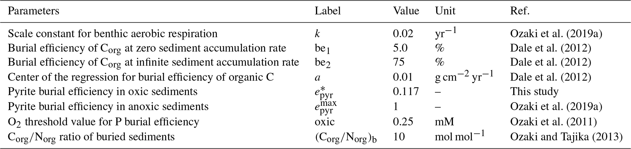
POM deposition

The fraction of settling POM that reaches the sediment surface, $J_{\mathrm{org}}^{\mathrm{dep}}$ (in mol C yr⁻¹) is a function of both the settling flux density, $j_{\mathrm{org}}^{\mathrm{dep}}$ (in mol C m⁻² yr⁻¹), and topography (Fig. 4a):

$$\begin{array}{}\text{(38)}& J_{\mathrm{org}}^{\mathrm{dep}}=\underset{z_{\mathrm{1}}}{\overset{z_{\mathrm{2}}}{\int }}{j}_{\mathrm{org}}^{\mathrm{dep}}\left(z\right){\displaystyle \frac{\mathrm{d}A}{\mathrm{d}z}}\mathrm{d}z,\end{array}$$

where the settling flux density can be written as follows:

$$\begin{array}{}\text{(39)}& j_{\mathrm{org}}^{\mathrm{dep}}=v_{\mathrm{POM}}G,\end{array}$$

where G is the concentration of POM and v_POM denotes the sinking velocity.

Carbon cycling

Interactions between the ocean and underlying sediments play an important role in influencing whole-ocean chemical and nutrient inventories on geologic timescales. POM deposited to the seafloor is subject to decomposition during diagenetic processes associated with burial in marine sediments. Only a small fraction of organic matter will ultimately be buried and removed from the surface environment. However, understanding what factors control the preservation of organic matter in marine sediments has been a controversial topic, and we still lack a robust understanding of this process. With this issue in mind, we adopt an empirical approach obtained using the observational data from previous studies.

The burial flux density of C_org at each water depth, $j_{\mathrm{org}}^{\mathrm{b},\mathrm{ocn}}$ (in terms of mol C m⁻² yr⁻¹), is calculated based on burial efficiency, BE_org:

$$\begin{array}{}\text{(40)}& j_{\mathrm{org}}^{\mathrm{b},\mathrm{ocn}}={\text{BE}}_{\mathrm{org}}{j}_{\mathrm{org}}^{\mathrm{dep}}.\end{array}$$

Burial efficiency is defined as the fraction of organic matter buried in sediments relative to the total depositional flux. Burial efficiency is described by simplified parametric laws based on empirical relationships from modern-day observations. Previous studies demonstrate strong dependency of this term on total sedimentation rate, SR (e.g., Henrichs and Reeburgh, 1987). Figure 6 demonstrates the relationship between BE_org and SR compiled from literature surveys. The sedimentation rate in the modern ocean varies over about 5 orders of magnitude, with a primary dependence on material supplied from the continents. There is a strong relationship, especially for SR less than 0.01 cm yr⁻¹. In contrast to the strong SR dependence under oxic conditions, anoxic settings show a much weaker dependence of BE_org on SR (Betts and Holland, 1991; Henrichs and Reeburgh, 1987) (Fig. 6). In this study, the following relationship proposed by Henrichs and Reeburgh (1987) is adopted for sediments underlying well-oxygenated bottom water (O₂ concentration of bottom water, [O₂]_bw>200 µM):

$$\begin{array}{}\text{(41)}& {\text{BE}}_{\mathrm{org}}={\displaystyle \frac{{\text{SR}}^{\mathrm{0.4}}}{\mathrm{2.1}}}.\end{array}$$

Given that BE_org depends on the [O₂]_bw (Lasaga and Ohmoto, 2002; Katsev and Crowe, 2015), we adopt the following formulation for sediments underlying less-oxygenated bottom waters ([O₂]_bw<30 µM) (Dale et al., 2012):

$$\begin{array}{}\text{(42)}& {\text{BE}}_{\mathrm{org}}=b_{\mathrm{2}}+{\displaystyle \frac{b_{\mathrm{1}}-b_{\mathrm{2}}}{\mathrm{1}+\text{SR}/a}},\end{array}$$

where a=0.019, b₁=0.05, and b₂=0.7, respectively. For intermediate [O₂]_bw levels, BE_org is evaluated as a function of [O₂]_bw with a log-linear interpolation method. Note that the original CANOPS model (Ozaki and Tajika, 2013; Ozaki et al., 2011) adopted Eq. (41) without considering the O₂ dependency, whereas more recent versions employ Eq. (42) for both oxic and anoxic sediments with different values of a, b₁, and b₂. In CANOPS-GRB v1.0, we adopted both equations because this provided a more accurate reproduction of C_org burial distribution in the modern ocean (Sect. 3.2.2).

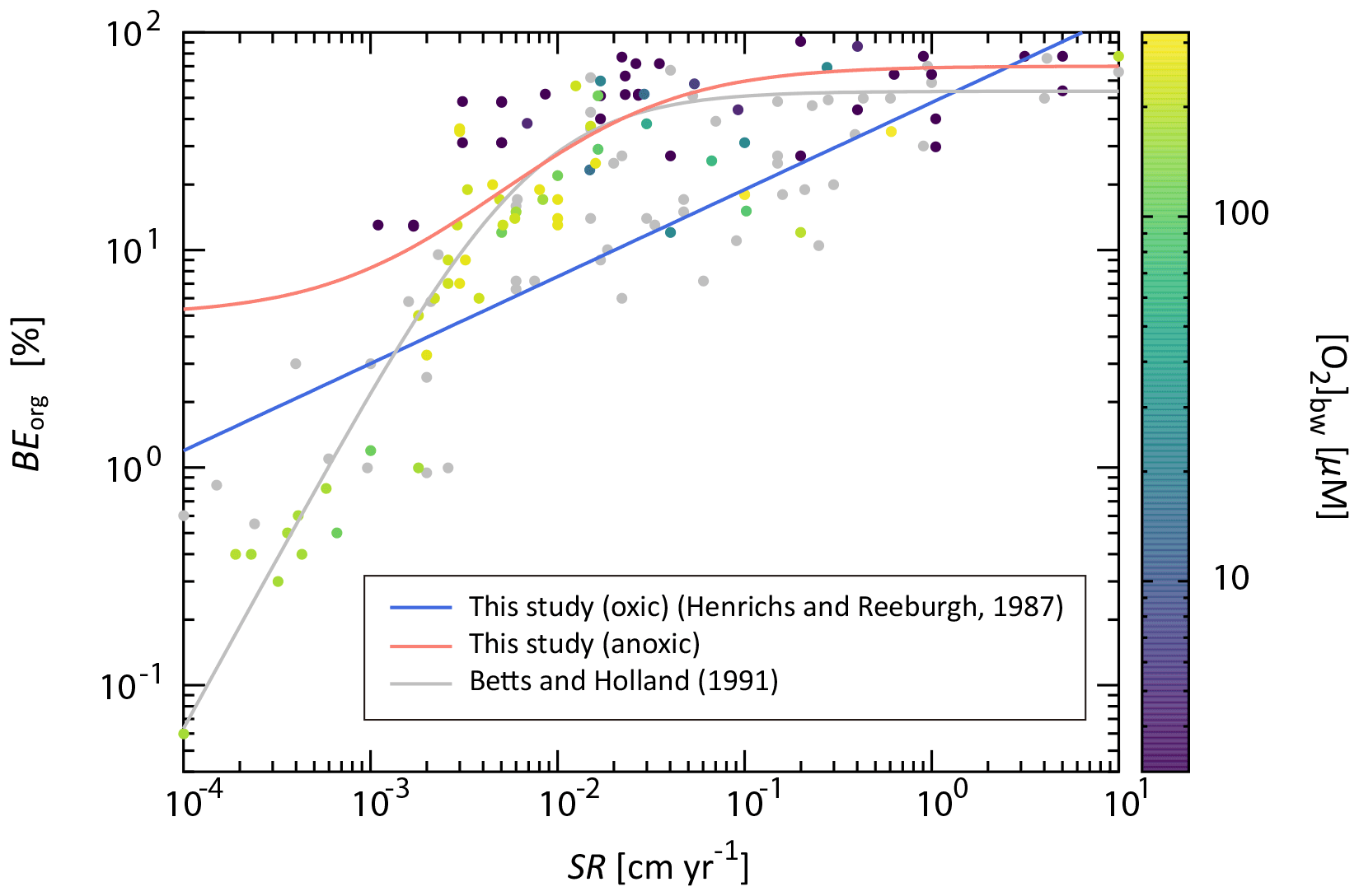
Figure 6 Burial efficiency of organic carbon (BE_org) as a function of sedimentation rate (SR). The dots denote the observational data compiled from literature survey (Betts and Holland, 1991; Canfield, 1993; Henrichs and Reeburgh, 1987; Tromp et al., 1995; Hartnett et al., 1998). The color represents the O₂ concentration of bottom water, [O₂]_bw, with gray dots for the unknown [O₂]_bw value. Blue and red lines are the relationship for well-oxygenated ([O₂]_bw>200 µM) (Henrichs and Reeburgh, 1987) and anoxic ([O₂]_bw<30 µM) marine sediments adopted in the CANOPS-GRB model, whereas the solid gray line is a previously proposed empirical relationship of Betts and Holland (1991).

Sedimentation rate depends strongly on water depth and distance from shore (Hedges et al., 1999), and we apply the relationship between water depth, z, and the reference value of SR shown by (Tromp et al., 1995) (Fig. 7).

$$\begin{array}{}\text{(43)}& z=\mathrm{2700}\times \text{erfc}\left(\mathrm{2.1}+\log {\text{SR}}^{\ast }\right).\end{array}$$

Using these formulas with seafloor topography (Fig. 4a) and $j_{\mathrm{org}}^{\mathrm{dep}}$ (Eq. 39), we can calculate $j_{\mathrm{org}}^{\mathrm{b},\mathrm{ocn}}$ for each ocean depth. In the CANOPS-GRB model, we also introduce an erosion factor, f_R, representing the global weathering and sedimentation rate (Sect. 2.5.3). Given the intimate coupling between global erosion rate and mass transfer from continents to the ocean, SR scales with the erosion factor (f_R=1 for our reference run):

$$\begin{array}{}\text{(44)}& \text{SR}\left(z\right)=f_{\mathrm{R}}\text{SR}(z{)}^{\ast }.\end{array}$$

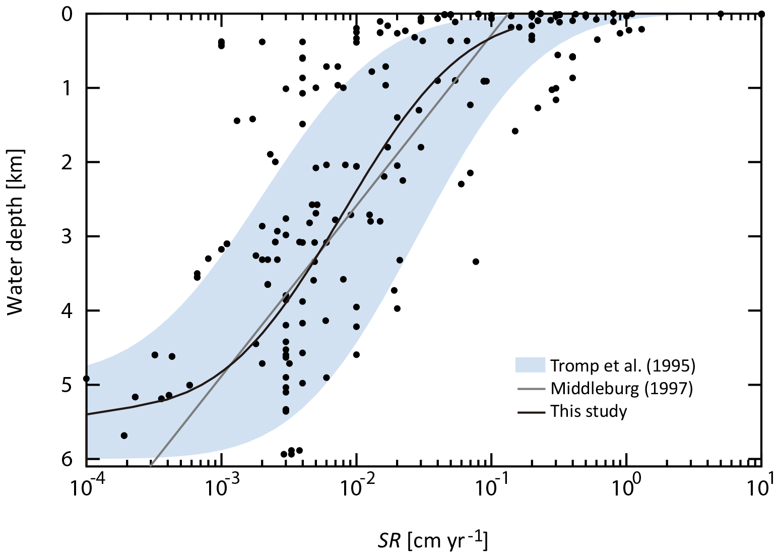
Figure 7 Sedimentation rate as a function of water depth. Data (black dots) were compiled from literature survey (Colman and Holland, 2000; Baturin, 2007; Betts and Holland, 1991; Tromp et al., 1995; Cha et al., 2005; Reimers et al., 1992). Black line represents the relationship assumed in the CANOPS-GRB model. Previously estimated empirical relationships (Middelburg et al., 1997; Tromp et al., 1995) are also shown.

Organic matter that is not buried is subject to decomposition. The benthic decomposition rate at each water depth is given as follows:

$$\begin{array}{}\text{(45)}& j_{\mathrm{recy}}^{\mathrm{sed}}=j_{\mathrm{org}}^{\mathrm{dep}}-j_{\mathrm{org}}^{\mathrm{b},\mathrm{ocn}}=\left(\mathrm{1}-{\text{BE}}_{\mathrm{org}}\right)j_{\mathrm{org}}^{\mathrm{dep}}.\end{array}$$

The respiration pathway used in the benthic decomposition is evaluated based on semi-empirical relationships obtained by 1-D early diagenesis models (see below). The fraction of aerobic degradation in total sedimentary respiration, f_aero, is calculated based on oxygen exposure time (τ_OET):

$$\begin{array}{}\text{(46)}& f_{\mathrm{aero}}=\left(\mathrm{1}-f_{\mathrm{deni}}\right)\left(\mathrm{1}-e^{-k{\mathit{\tau }}_{\mathrm{OET}}}\right),\end{array}$$

where f_deni denotes the fraction of denitrification and k is an empirical constant. τ_OET is given by

$$\begin{array}{}\text{(47)}& {\mathit{\tau }}_{\mathrm{OET}}={\displaystyle \frac{\text{OPD}}{\text{SR}}},\end{array}$$

where OPD is the oxygen penetration depth (cm) and SR denotes a linear sedimentation rate (cm yr⁻¹). In the CANOPS-GRB model OPD is calculated by a simplified parametric law obtained from a 1-D early diagenetic model of C and O₂. We performed a series of experiments (n=5652) in order to parameterize OPD as a polynomial function with the following variables: sedimentation rate SR (cm yr⁻¹), bottom-water O₂ concentration [O₂]_bw (µM), depositional flux of POC $j_{\mathrm{org}}^{\mathrm{dep}}$ (mmol C cm⁻² yr⁻¹), and bottom water temperature T_bw (^∘C). The variables are allowed to vary over a parameter space spanning 10⁻⁴ cm yr${}^{-\mathrm{1}}<\text{SR}<{\mathrm{10}}^{\mathrm{1}}$ cm yr⁻¹, 10⁰ µM < [O₂]_bw<10³ µM, 10⁻⁴ mmol C cm⁻² yr${}^{-\mathrm{1}}<j_{\mathrm{org}}^{\mathrm{dep}}<{\mathrm{10}}^{\mathrm{1}}$ mmol C cm⁻² yr⁻¹, and 0 ^∘C $<T_{\mathrm{bw}}<\mathrm{30}$ ^∘C.

$$\begin{array}{}\text{(48)}& \begin{array}{rl}\log \text{OPD}& =a_{\mathrm{0}}+a_{\mathrm{1}}\log \text{SR}+a_{\mathrm{2}}\log [{\mathrm{O}}_{\mathrm{2}}{]}_{\mathrm{bw}}\\ & +a_{\mathrm{3}}\log j_{\mathrm{org}}^{\mathrm{dep}}+a_{\mathrm{4}}(\log \text{SR}{)}^{\mathrm{2}}\\ & +a_{\mathrm{5}}\left(\log \right[{\mathrm{O}}_{\mathrm{2}}{]}_{\mathrm{bw}}{)}^{\mathrm{2}}+a_{\mathrm{6}}(\log j_{\mathrm{org}}^{\mathrm{dep}}{)}^{\mathrm{2}}\\ & +a_{\mathrm{7}}\left(\log \text{SR}\right)\left(\log \right[{\mathrm{O}}_{\mathrm{2}}{]}_{\mathrm{bw}})\\ & +a_{\mathrm{8}}\left(\log \right[{\mathrm{O}}_{\mathrm{2}}{]}_{\mathrm{bw}}\left)\right(\log j_{\mathrm{org}}^{\mathrm{dep}})\\ & +a_{\mathrm{9}}\left(\log SR\right)\left(\log j_{\mathrm{org}}^{\mathrm{dep}}\right)+a_{\mathrm{10}}{T}_{\mathrm{bw}},\end{array}\end{array}$$

where $a_{\mathrm{0}}=-\mathrm{2.24869}$, a₁=0.110645, a₂=1.12569, $a_{\mathrm{3}}=-\mathrm{0.281005}$, a₄=0.014827, $a_{\mathrm{5}}=-\mathrm{0.124721}$, a₆=0.0894604, a₇=0.00279531, $a_{\mathrm{8}}=-\mathrm{0.127797}$, a₉=0.0017995, and a₁₀=0.0085171. This parametric fit provides a rapid means of obtaining OPD from a 1-D early diagenetic model of C and O₂ (Fig. 8). Note that Eq. (48) is verified for [O₂]_bw>1 µM. When bottom water O₂ concentration is lower than 1 µM, OPD is set at zero.

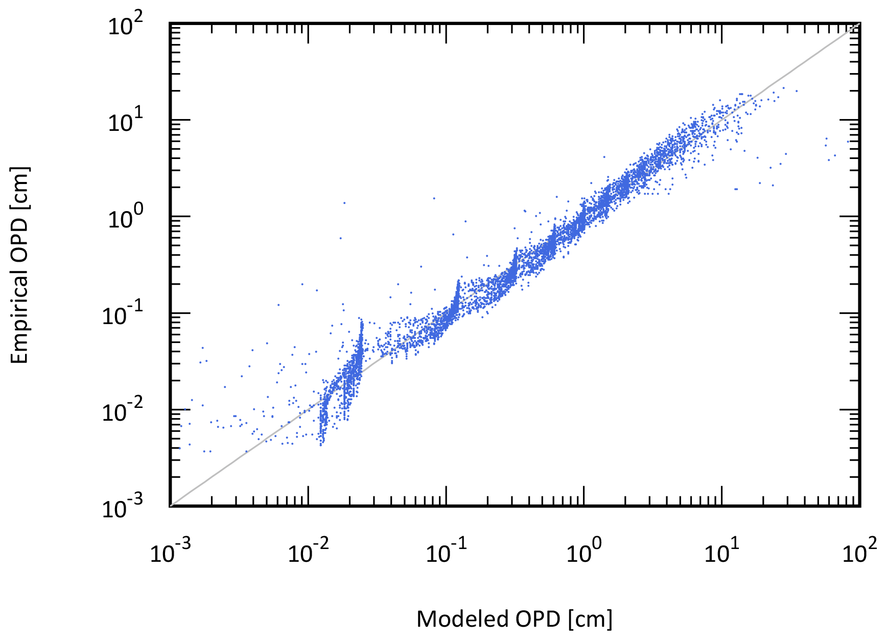
Figure 8 The correlation between the simulated OPD and the OPD obtained from an empirical relationship of Eq. (48) (n=5652). The gray line denotes the 1:1 line (r²=0.9595).

Phosphorus cycling

Marine P inventory is controlled not only by the riverine P input flux from land but also by the efficiency of P recycling in marine sediments (Van Cappellen and Ingall, 1994). Because the estimated P diffusive flux from seafloor sediments is much greater than the riverine P flux (Delaney, 1998; Hensen et al., 1998; Ruttenberg, 2003; McManus et al., 1997; Wallmann, 2003, 2010), changes in diagenetic processes affecting P recycling and burial in marine sediments could have a significant impact on global oceanic biogeochemical cycles.

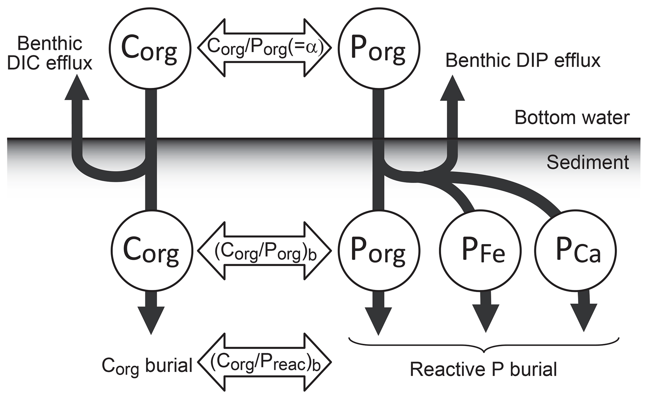
Figure 9 Schematic of P burial in marine sediments. The primary source of P to the sediment is the deposition of organic matter, which represents the C:P ratio of primary producers, α. Phosphorus deposited in sediments is a subject of decomposition and sink switching. Most of the deposited organic P is decomposed before burial and the DIP released to pore waters diffuses to the bottom water. A fraction of the liberated P is trapped by iron hydroxides or buried as authigenic minerals (e.g., carbonate fluorapatite). Three reactive phases, organic P (P_org), Fe-bound P (P_Fe), and Ca-bound P (P_Ca), are considered in the CANOPS-GRB model. The burial of these species are redox dependent: burial efficiency is affected by bottom water O₂ concentration. Because of the sink switching, sedimentary ${\mathrm{C}}_{\mathrm{org}}/{\mathrm{P}}_{\mathrm{reac}}$, rather than ${\mathrm{C}}_{\mathrm{org}}/{\mathrm{P}}_{\mathrm{org}}$ ratios, provides a correct measure of the retention vs. diffusive loss of remineralized P.

A schematic of benthic P cycling is shown in Fig. 9. The majority of organic matter delivered to the sediment–water interface is regenerated (Jahnke, 1996), but a fraction of DIP released via respiration to pore waters is redistributed to other phases such as iron hydroxide or carbonate fluorapatite within the sediments. This mechanism is known as “sink-switching” (e.g., Anderson et al., 2001; Filippelli, 2001), and results in P burial other than organic P playing a more important role in the total P sink (Ruttenberg, 1993, 2003; Compton et al., 2000). Three different P pools are considered in the CANOPS-GRB model: organic P (P_org), Fe-hydroxide-bound P (P_Fe), and authigenic Ca-bound P (P_Ca). The sum of these pools is defined as biologically reactive P (P_reac) (bioavailable in the ocean to fuel primary productivity). The marine C and P cycles are coupled not only through the ${\mathrm{C}}_{\mathrm{org}}/{\mathrm{P}}_{\mathrm{org}}$ ratio of POM (α) but also through the ${\mathrm{C}}_{\mathrm{org}}/{\mathrm{P}}_{\mathrm{reac}}$ ratio of marine sediments. It is important to note that, as argued by Anderson et al. (2001), the fundamental measure of the retention vs. diffusive loss of remineralized P is not the sedimentary ${\mathrm{C}}_{\mathrm{org}}/{\mathrm{P}}_{\mathrm{org}}$ ratio but the ratio of ${\mathrm{C}}_{\mathrm{org}}/{\mathrm{P}}_{\mathrm{reac}}$.

Field observations of marine and lacustrine sediments have revealed that the burial efficiency of P depends on the redox conditions of bottom waters (Ingall and Jahnke, 1994): phosphorus retention potential is suppressed under anoxic bottom water conditions. Elevated ${\mathrm{C}}_{\mathrm{org}}/{\mathrm{P}}_{\mathrm{reac}}$ ratios observed in permanently anoxic environments suggest preferential regeneration of P relative to C under these conditions (Algeo and Ingall, 2007; Anderson et al., 2001; Colman and Holland, 2000; Filippelli, 2001; Ingall and Jahnke, 1997). In the CANOPS-GRB model, P benthic regeneration rate is calculated at each sediment segment based on the POP depositional flux density $j_{\mathrm{P}}^{\mathrm{dep}}(=j_{\mathrm{org}}^{\mathrm{dep}}/\mathit{\alpha })$ and P burial efficiency, which is a function of both [O₂]_bw and SR. We assume the following formulation for the ${\mathrm{C}}_{\mathrm{org}}/{\mathrm{P}}_{\mathrm{org}}$ ratio of the buried organic phase on the basis of previous studies (Slomp and Van Cappellen, 2007; Van Cappellen and Ingall, 1994, 1996):

$$\begin{array}{}\text{(49)}& ({\mathrm{C}}_{\mathrm{org}}/{\mathrm{P}}_{\mathrm{org}}{)}_{\mathrm{b}}=\left\{\begin{array}{l}\frac{({\mathrm{C}}_{\mathrm{org}}/{\mathrm{P}}_{\mathrm{org}}{)}_{\mathrm{b}}^{\mathrm{oxic}}({\mathrm{C}}_{\mathrm{org}}/{\mathrm{P}}_{\mathrm{org}}{)}_{\mathrm{b}}^{\mathrm{anox}}}{({\mathrm{C}}_{\mathrm{org}}/{\mathrm{P}}_{\mathrm{org}}{)}_{\mathrm{b}}^{\mathrm{anox}}\frac{[{\mathrm{O}}_{\mathrm{2}}{]}_{\mathrm{bw}}}{\mathrm{oxic}}+\left(\mathrm{1}-\frac{[{\mathrm{O}}_{\mathrm{2}}{]}_{\mathrm{bw}}}{\mathrm{oxic}}\right)({\mathrm{C}}_{\mathrm{org}}/{\mathrm{P}}_{\mathrm{org}}{)}_{\mathrm{b}}^{\mathrm{oxic}}}{f}_{\mathit{\tau }}\\ \text{for }{\left[{\mathrm{O}}_{\mathrm{2}}\right]}_{\mathrm{bw}}<\text{oxic}\\ ({\mathrm{C}}_{\mathrm{org}}/{\mathrm{P}}_{\mathrm{org}}{)}_{\mathrm{b}}^{\mathrm{oxic}}{f}_{\mathit{\tau }}\\ \text{for }{\left[{\mathrm{O}}_{\mathrm{2}}\right]}_{\mathrm{bw}}\ge \text{oxic}\end{array}\right.,\end{array}$$

where $({\mathrm{C}}_{\mathrm{org}}/{\mathrm{P}}_{\mathrm{org}}{)}_{\mathrm{b}}^{\mathrm{oxic}}$ and $({\mathrm{C}}_{\mathrm{org}}/{\mathrm{P}}_{\mathrm{org}}{)}_{\mathrm{b}}^{\mathrm{anox}}$ denote organic C/P ratios for fully oxic and anoxic conditions and oxic (=250 µM) is a threshold value of [O₂]_bw below which preferential P regeneration occurs. $({\mathrm{C}}_{\mathrm{org}}/{\mathrm{P}}_{\mathrm{org}}{)}_{\mathrm{b}}^{\mathrm{oxic}}$ is set to twice the value of the Redfield ratio, and $({\mathrm{C}}_{\mathrm{org}}/{\mathrm{P}}_{\mathrm{org}}{)}_{\mathrm{b}}^{\mathrm{anox}}$ is an upper limit assumed for organic matter buried under fully anoxic overlying waters, estimated as 40 times larger than the Redfield value on the basis of previous studies on various ancient anoxic basin sediments (Slomp and Van Cappellen, 2007; Ingall et al., 1993). In Eq. (49), we also include the dependence of buried ${\mathrm{C}}_{\mathrm{org}}/{\mathrm{P}}_{\mathrm{org}}$ ratio on SR, expressed as f_τ. Modern observations suggest that SR is a one of the major factors influencing the preservation vs. remineralization of sedimentary organic C and P. Organic C preservation in marine sediments tends to be enhanced at higher SR. In contrast, the ${\mathrm{C}}_{\mathrm{org}}/{\mathrm{P}}_{\mathrm{org}}$ ratio of sedimentary organic matter shows a nonlinear relationship with respect to SR (Ingall and Cappellen, 1990) (Sect. 3.2.3), suggesting more complex behavior of benthic P cycling. Specifically, in the pelagic deep ocean, preferential P regeneration is not observed, likely due to the long timescale of diagenesis prior to burial (Ingall and Cappellen, 1990). In the CANOPS model, f_τ is formulated as follows:

$$\begin{array}{}\text{(50)}& f_{\mathit{\tau }}=\mathrm{0.5}+\mathrm{0.5}\exp \left(-{\displaystyle \frac{\mathrm{0.001}\mathrm{cm}}{\text{SR}}}\right).\end{array}$$

Specifically, the ${\mathrm{C}}_{\mathrm{org}}/{\mathrm{P}}_{\mathrm{org}}$ ratio approaches the Redfield value for oxygenated pelagic sediments.

The burial flux density of P_org can be calculated as the C_org burial flux density divided by $({\mathrm{C}}_{\mathrm{org}}/{\mathrm{P}}_{\mathrm{org}}{)}_{\mathrm{b}}$:

$$\begin{array}{}\text{(51)}& j_{{\mathrm{P}}_{\mathrm{org}}}^{\mathrm{b}}={\displaystyle \frac{j_{\mathrm{org}}^{\mathrm{b},\mathrm{ocn}}}{{\left({\mathrm{C}}_{\mathrm{org}}/{\mathrm{P}}_{\mathrm{org}}\right)}_{\mathrm{b}}}}.\end{array}$$

The burial efficiency of P_org can be written as follows:

$$\begin{array}{}\text{(52)}& {\text{BE}}_{{\mathrm{P}}_{\mathrm{org}}}\equiv {\displaystyle \frac{j_{{\mathrm{P}}_{\mathrm{org}}}^{\mathrm{b}}}{j_{\mathrm{P}}^{\mathrm{dep}}}}={\displaystyle \frac{j_{{\mathrm{P}}_{\mathrm{org}}}^{\mathrm{b}}}{j_{\mathrm{org}}^{\mathrm{dep}}/\mathit{\alpha }}}={\displaystyle \frac{\mathit{\alpha }{\text{BE}}_{\mathrm{org}}}{j_{\mathrm{org}}^{\mathrm{b}}/j_{{\mathrm{P}}_{\mathrm{org}}}^{\mathrm{b}}}}={\displaystyle \frac{\mathit{\alpha }{\text{BE}}_{\mathrm{org}}}{{\left({\mathrm{C}}_{\mathrm{org}}/{\mathrm{P}}_{\mathrm{org}}\right)}_{\mathrm{b}}}},\end{array}$$

where $j_{\mathrm{P}}^{\mathrm{dep}}$ denotes the POP settling flux density to sediments, which is coupled to the $\mathrm{C}/\mathrm{P}$ stoichiometry of POM ($=j_{\mathrm{org}}^{\mathrm{dep}}/\mathit{\alpha }$).

Under oxic bottom-water conditions, remineralized organic P can be trapped efficiently at the sediment–water interface by ferric iron phases. In contrast, under anoxic bottom water conditions, a lack of ferric iron phases allows most mineralized P to diffuse out of the sediment. This redox-dependent P burial is assumed to be linearly proportional to the [O₂]_bw (Slomp and Van Cappellen, 2007):

$$\begin{array}{}\text{(53)}& j_{\mathrm{P}-\mathrm{Fe}}^{\mathrm{b}}=\left\{\begin{array}{ll}{\text{BE}}_{{\mathrm{P}}_{\mathrm{org}}}^{\mathrm{oxic}}\left(\frac{[{\mathrm{O}}_{\mathrm{2}}{]}_{\mathrm{bw}}}{\text{oxic}}\right)j_{{\mathrm{P}}_{\mathrm{org}}}^{\mathrm{dep}}& \text{ for }[{\mathrm{O}}_{\mathrm{2}}{]}_{\mathrm{bw}}<\text{oxic}\\ {\text{BE}}_{{\mathrm{P}}_{\mathrm{org}}}^{\mathrm{oxic}}{j}_{{\mathrm{P}}_{\mathrm{org}}}^{\mathrm{dep}}& \text{ for }[{\mathrm{O}}_{\mathrm{2}}{]}_{\mathrm{bw}}\ge \text{oxic}\end{array}\right.,\end{array}$$

where BE${}_{{\mathrm{P}}_{\mathrm{org}}}^{\mathrm{oxic}}$ denotes the burial efficiency of P_org under well-oxygenated bottom water conditions ([O₂]_bw>oxic). We assume that the retention potential of P_Fe in sediments overlain by oxic bottom waters is comparable to that of P_org (Ruttenberg, 1993).

Some authors have also proposed that authigenic P burial, the dominant process for P burial today (Ruttenberg, 1993), depends on the redox conditions of the bottom water (Slomp and Van Cappellen, 2007; Slomp et al., 2002). In the CANOPS-GRB model, we adopt the following redox dependence used by Slomp and Van Cappellen (2007):

$$\begin{array}{}\text{(54)}& j_{\mathrm{P}-\mathrm{Ca}}^{\mathrm{b}}=\left\{\begin{array}{l}\mathrm{2}{\text{BE}}_{{\mathrm{P}}_{\mathrm{org}}}^{\mathrm{oxic}}\left(a_{\mathrm{auth}}+\left(\mathrm{1}-a_{\mathrm{auth}}\right)\frac{[{\mathrm{O}}_{\mathrm{2}}{]}_{\mathrm{bw}}}{\text{oxic}}\right)j_{{\mathrm{P}}_{\mathrm{org}}}^{\mathrm{dep}}\\ \text{for }[{\mathrm{O}}_{\mathrm{2}}{]}_{\mathrm{bw}}<\text{oxic}\\ \mathrm{2}{\text{BE}}_{{\mathrm{P}}_{\mathrm{org}}}^{\mathrm{oxic}}{j}_{{\mathrm{P}}_{\mathrm{org}}}^{\mathrm{dep}}\\ \text{for }[{\mathrm{O}}_{\mathrm{2}}{]}_{\mathrm{bw}}\ge \text{oxic}\end{array}\right..\end{array}$$

We assume that P_org, P_Fe and P_Ca account roughly for 25 %, 25 %, and 50 %, respectively, of the total reactive P buried in oxygenated sediments (Ruttenberg, 1993). Therefore, the burial efficiency of authigenic P phases is larger than that of P_org and P_Fe by a factor of 2. The redox dependency of authigenic P burial is controlled by a parameter, a_auth. There is still great uncertainty as to the sensitivity of P retention efficiency of authigenic P phases to changing redox conditions. For instance, a recent modeling study suggests that the burial of authigenic P is influenced not only by the redox state of bottom water but also by seawater chemistry (especially Ca²⁺) (Zhao et al., 2020), temperature, and pH (Papadomanolaki et al., 2022). In our reference run, we set a_auth at 1, i.e., no redox dependency for authigenic P burial.

When above formulations are adopted, the ratio

$$\begin{array}{}\text{(55)}& \stackrel{\mathrm{‾}}{{\mathrm{C}}_{\mathrm{org}}/{\mathrm{P}}_{\mathrm{reac}}}={\displaystyle \frac{\mathrm{Marine}{\mathrm{C}}_{\mathrm{org}}\text{ burial rate}}{\mathrm{Marine}{\mathrm{P}}_{\mathrm{reac}}\text{ burial rate}}},\end{array}$$

varies between 63 and 370 as a function of ocean redox state. This is in the range of an estimation derived from various observations of modern and ancient sediments (Papadomanolaki et al., 2022; Algeo and Ingall, 2007). Given that the continental shelves are a main locus of reactive P burial, the separate treatment of continental shelves and margin sediments from the pelagic ocean could affect the nonlinearity of the redox-dependent P cycle. However, this was left as one of the subjects of future work.

Nitrogen cycling

The benthic denitrification rate is estimated with a semi-empirical relationship (Middelburg et al., 1996). Middelburg and colleagues performed a series of experiments (n=2000) with a 1-D early diagenetic model of C–N–O₂ to parameterize benthic denitrification $j_{\mathrm{deni}}^{\mathrm{sed}}$ ($\mathrm{\mu }\mathrm{mol}\mathrm{C}{\mathrm{cm}}^{-\mathrm{2}}{\mathrm{d}}^{-\mathrm{1}}$) as a polynomial function using $j_{\mathrm{org}}^{\mathrm{dep}}$ ($\mathrm{\mu }\mathrm{mol}\mathrm{C}{\mathrm{cm}}^{-\mathrm{2}}{\mathrm{d}}^{-\mathrm{1}}$), z (m), and bottom-water concentrations of dissolved O₂ and NO${}_{\mathrm{3}}^{-}$ (µM):

$$\begin{array}{}\text{(56)}& \begin{array}{rl}\log j_{\mathrm{deni}}^{\mathrm{sed}}& =c_{\mathrm{0}}+c_{\mathrm{1}}\log j_{\mathrm{org}}^{\mathrm{dep}}+c_{\mathrm{2}}{\left(\log j_{\mathrm{org}}^{\mathrm{dep}}\right)}^{\mathrm{2}}\\ & +c_{\mathrm{3}}\log \left[{\mathrm{NO}}_{\mathrm{3}}^{-}{]}_{\mathrm{bw}}\log \right[{\mathrm{O}}_{\mathrm{2}}{]}_{\mathrm{bw}}\\ & +c_{\mathrm{4}}\log [{\mathrm{NO}}_{\mathrm{3}}^{-}{]}_{\mathrm{bw}}+c_{\mathrm{5}}\log [{\mathrm{O}}_{\mathrm{2}}{]}_{\mathrm{bw}}+c_{\mathrm{6}}\log z\\ & +c_{\mathrm{7}}\log j_{\mathrm{org}}^{\mathrm{dep}}\log [{\mathrm{O}}_{\mathrm{2}}{]}_{\mathrm{bw}},\end{array}\end{array}$$

where $c_{\mathrm{0}}=-\mathrm{2.2567}$, $c_{\mathrm{1}}=-\mathrm{0.1850}$, $c_{\mathrm{2}}=-\mathrm{0.2210}$, $c_{\mathrm{3}}=-\mathrm{0.3995}$, c₄=1.2500, c₅=0.4721, and $c_{\mathrm{6}}=-\mathrm{0.0996}$, c₇=0.4256. This polynomial function was obtained by examining a parameter space spanning 50 m $<z<\mathrm{6000}$ m, 10 µM < [O₂]_bw<350 µM, and 1 µM < [NO${}_{\mathrm{3}}^{-}$]_bw<60 µM. $j_{\mathrm{org}}^{\mathrm{dep}}$ was allowed to vary within 2 orders of magnitude at each water depth (Middelburg et al., 1996). As pointed out by Romaniello and Derry (2010), the predicted contribution of denitrification to total decomposition f_deni ($=j_{\mathrm{denitr}}^{\mathrm{sed}}/j_{\mathrm{recy}}^{\mathrm{sed}}$) can sometimes exceed 100 % for [O₂]_bw<10 µM. When the fraction of benthic denitrification to total decomposition exceeds 90 %, benthic denitrification is limited in order to avoid unphysical values (Ozaki and Tajika, 2013; Romaniello and Derry, 2010).

The burial flux density of N_org is calculated by molar ratio of C to N of buried sediments, (C_org $/$ N_org)_b, and the burial flux of C_org:

$$\begin{array}{}\text{(57)}& j_{{\mathrm{N}}_{\mathrm{org}}}^{\mathrm{b}}={\displaystyle \frac{j_{\mathrm{org}}^{\mathrm{b},\mathrm{ocn}}}{{\left({\mathrm{C}}_{\mathrm{org}}/{\mathrm{N}}_{\mathrm{org}}\right)}_{\mathrm{b}}}}.\end{array}$$

We assumed an average ratio of 10, which is observed in the Washington and Mexico margin (Hedges et al., 1999; Hartnett and Devol, 2003).

Sulfur cycling

The fractions of MSR and methanogenesis to total decomposition of organic matter in marine sediment are given by

$$\begin{array}{}\text{(58)}& {\displaystyle }{f}_{\mathrm{MSR}}=\left(\mathrm{1}-f_{\mathrm{aerobic}}-f_{\mathrm{denitr}}\right){\displaystyle \frac{[{\mathrm{SO}}_{\mathrm{4}}^{\mathrm{2}-}{]}_{\mathrm{bw}}}{[{\mathrm{SO}}_{\mathrm{4}}^{\mathrm{2}-}{]}_{\mathrm{bw}}+K_{\mathrm{MSR}}}},\text{(59)}& {\displaystyle }{f}_{\mathrm{meth}}=\mathrm{1}-f_{\mathrm{aero}}-f_{\mathrm{deni}}-f_{\mathrm{MSR}}.\end{array}$$

The production rate of hydrogen sulfide in sediment, $j_{{\mathrm{H}}_{\mathrm{2}}\mathrm{S}}^{\mathrm{sed}}$ (mol S m⁻² yr⁻¹), is given by

$$\begin{array}{}\text{(60)}& j_{{\mathrm{H}}_{\mathrm{2}}\mathrm{S}}^{\mathrm{sed}}={\displaystyle \frac{\mathrm{1}}{\mathrm{2}}}{f}_{\mathrm{MSR}}{j}_{\mathrm{recy}}^{\mathrm{sed}}+j_{\mathrm{AOM}},\end{array}$$

where j_AOM denotes the production rate of sulfide via AOM:

$$\begin{array}{}\text{(61)}& j_{\mathrm{AOM}}={\displaystyle \frac{\mathrm{1}}{\mathrm{2}}}{f}_{\mathrm{meth}}{\displaystyle \frac{[{\mathrm{SO}}_{\mathrm{4}}^{\mathrm{2}-}{]}_{\mathrm{bw}}}{[{\mathrm{SO}}_{\mathrm{4}}^{\mathrm{2}-}{]}_{\mathrm{bw}}+K_{\mathrm{MSR}}}}{j}_{\mathrm{recy}}^{\mathrm{sed}}.\end{array}$$

Here we assume that AOM is proportional to the CH₄ production rate with a sulfate-dependent term.

The rate of pyrite precipitation in sediments would be proportional to the sulfide production rate at the sediment-water interface:

$$\begin{array}{}\text{(62)}& j_{\mathrm{pyr}}^{\mathrm{b},\mathrm{sed}}=e_{\mathrm{pyr}}{j}_{{\mathrm{H}}_{\mathrm{2}}\mathrm{S}}^{\mathrm{sed}},\end{array}$$

where the proportional coefficient, e_pyr, is the pyrite burial efficiency. The rate of MSR is a function of the marine redox state, [SO${}_{\mathrm{4}}^{\mathrm{2}-}$], and the availability of degradable organic matter. In well-oxygenated modern oceans most sulfide produced in sediments is re-oxidized and only a few percent of total sulfide is buried as pyrite (Canfield, 1991; Lin and Morse, 1991; Turchyn and Schrag, 2004; Bowles et al., 2014; Jørgensen, 1982). It has been pointed out that efficient oxidation of sulfide is promoted by animal bioturbation (Berner and Westrich, 1985; Canfield and Farquhar, 2009). In contrast, the value of e_pyr for anoxic sediments is much greater due to the absence of bioturbation and enhanced sulfide production. We assume that e_pyr asymptotes toward unity with decreasing the bottom water [O₂] (Tarhan et al., 2015):

$$\begin{array}{}\text{(63)}& e_{\mathrm{pyr}}=e_{\mathrm{pyr}}^{\max }-\left(e_{\mathrm{pyr}}^{\max }-e_{\mathrm{pyr}}^{\ast }\right)\tanh [{\mathrm{O}}_{\mathrm{2}}{]}_{\mathrm{bw}},\end{array}$$

where $e_{\mathrm{pyr}}^{\max }$ (=1 in our reference run) denotes the maximum pyrite precipitation efficiency in anoxic sediments. The reference value, $e_{\mathrm{pyr}}^{\ast }$, was calibrated using a present-day control simulation such that the present-day seawater [SO${}_{\mathrm{4}}^{\mathrm{2}-}$] is ∼29 mM. The obtained value of 0.117 is generally consistent with modern observations (Bottrell and Newton, 2006; Tarhan et al., 2015; Turchyn and Schrag, 2006) (see Sect. 3.2.5). Although our approach does not provide a mechanistic description of the complex process of pyrite precipitation, it is suitable for many purposes.

Early diagenetic modeling for quantifying the OPD

A simple 1-D early diagenetic model of C and O₂ is employed to obtain the parameterization of OPD (Eq. 48). The 100 cm thick sediment is vertically divided into 50 layers with an uneven grid. The grid size increases from the sediment–water interface (Δz=0.25 mm) to the maximum simulated sediment depth (Δz=1.6 cm). The diagenetic model calculates transport and biogeochemical transformation processes at each grid point within these sediment columns as well as the sedimentary burial and recycling fluxes at the model boundaries. The one-dimensional mass conservation equation for POC (wt. %) and dissolved O₂ is given by

$$\begin{array}{}\text{(64)}& {\displaystyle \frac{\partial \mathrm{POC}}{\partial t}}=D_{\mathrm{bio}}{\displaystyle \frac{{\partial }^{\mathrm{2}}\mathrm{POC}}{\partial z^{\mathrm{2}}}}-\text{SR}{\displaystyle \frac{\partial \text{POC}}{\partial z}}-k\text{POC},\text{(65)}& {\displaystyle }\begin{array}{rl}{\displaystyle \frac{\partial \left[{\mathrm{O}}_{\mathrm{2}}\right]}{\partial t}}& =D_{{\mathrm{O}}_{\mathrm{2}}}{\displaystyle \frac{{\partial }^{\mathrm{2}}{[\mathrm{O}}_{\mathrm{2}}]}{\partial z^{\mathrm{2}}}}-r_{{\mathrm{O}}_{\mathrm{2}}}k\text{POC}\\ & \cdot \left({\displaystyle \frac{\mathit{\rho }(\mathrm{1}-\mathit{\phi })}{\mathrm{1.2}\mathit{\phi }}}\right){\displaystyle \frac{\left[{\mathrm{O}}_{\mathrm{2}}\right]}{\left[{\mathrm{O}}_{\mathrm{2}}\right]+K_{{\mathrm{O}}_{\mathrm{2}}}}},\end{array}\end{array}$$

where $D_{{\mathrm{O}}_{\mathrm{2}}}$ is the diffusion coefficient of O₂, SR is the sedimentation rate, and φ is porosity, which is assumed to be constant over the entire sediment column for simplicity. Bioturbation is formulated as a diffusive process with a coefficient D_bio. The effective diffusion coefficient of O₂ is then given by

$$\begin{array}{}\text{(66)}& D_{{\mathrm{O}}_{\mathrm{2}}}={\displaystyle \frac{D_{{\mathrm{O}}_{\mathrm{2}}}^{T=\mathrm{0}}\times \left(\mathrm{1}+{\mathit{\nu }}_{{\mathrm{O}}_{\mathrm{2}}}{T}_{\mathrm{bw}}\right)}{{\mathit{\theta }}^{\mathrm{2}}}}+D_{\mathrm{bio}},\end{array}$$

where $D_{{\mathrm{O}}_{\mathrm{2}}}^{T=\mathrm{0}}$ denotes a tracer diffusion coefficient in seawater of 0 ^∘C and $v_{{\mathrm{O}}_{\mathrm{2}}}$ is a coefficient for temperature dependence of molecular diffusion coefficient. The in situ diffusion coefficient is further corrected for tortuosity θ, which is related to pore water resistivity and porosity via the following expressions (Colman and Holland, 2000; Tromp et al., 1995; Berner, 1980):

$$\begin{array}{}\text{(67)}& {\displaystyle }{\mathit{\theta }}^{\mathrm{2}}=\mathit{\phi }F,\text{(68)}& {\displaystyle }F={\mathit{\phi }}^{-m},\end{array}$$

where F is the formation factor – defined as the ratio of bulk sediment resistivity to interstitial water resistivity – and m is an empirical constant, varying with sediment type. We assumed the average value for unconsolidated muds (m=2.7) in this work (Tromp et al., 1995). The particle mixing coefficient for bioturbation D_bio is formulated as a function of both sediment accumulation rate and bottom-water O₂ concentration (Tromp et al., 1995; Wallmann, 2003):

$$\begin{array}{}\text{(69)}& D_{\mathrm{bio}}={\mathrm{10}}^{\mathrm{1.63}+\mathrm{0.85}\log \text{SR}}{\displaystyle \frac{[{\mathrm{O}}_{\mathrm{2}}{]}_{\mathrm{bw}}}{[{\mathrm{O}}_{\mathrm{2}}{]}_{\mathrm{bw}}+K_{{\mathrm{O}}_{\mathrm{2}}}}}.\end{array}$$

At the bottom of the sediment column, a no-flux condition was applied. The parameters used in the 1-D early diagenetic model are tabulated in Table 6.

Table 6 Parameters used in the 1-D early diagenetic model.

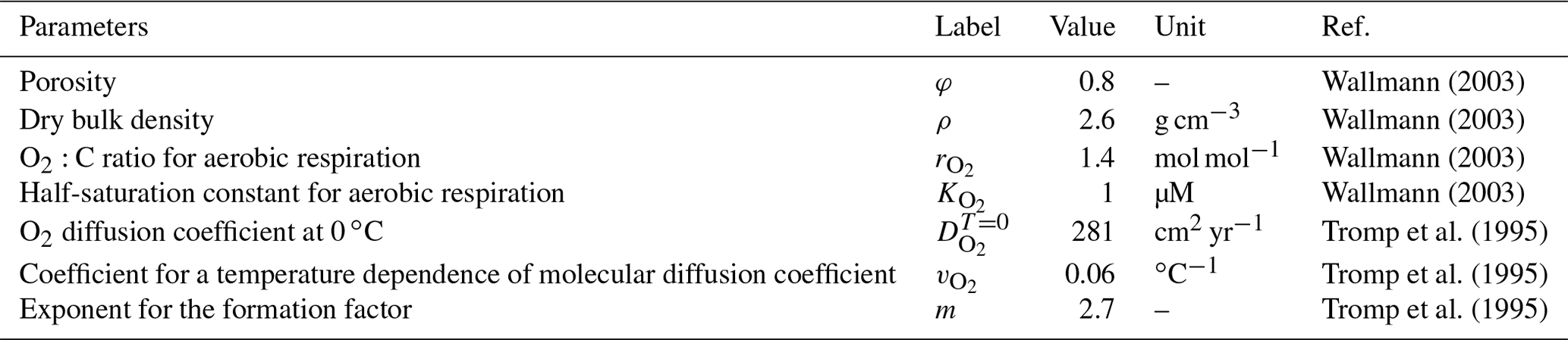
2.4.5 Air–sea exchange

To calculate the gas exchange of O₂, H₂S, NH₃, and CH₄ across the air–sea interface, we employed a stagnant film model (Liss and Slater, 1974). The flux of a gas X across the air–sea interface is controlled by the difference in partial pressure between the atmosphere and surface waters, which can be described by the following formula:

$$\begin{array}{}\text{(70)}& J_X^{\mathrm{air}-\mathrm{sea}}=v_X^{\mathrm{pis}}\left([X{]}_{\mathrm{aq}}-[X{]}_{\mathrm{sat}}\right),\end{array}$$

where $v_X^{\mathrm{pis}}$, [X]_aq, and [X]_sat denote piston velocity, the dissolved concentration of species X, and the saturation concentration of species X, respectively. For O₂, the saturation concentration is calculated based on solubility (Garcia and Gordon, 1992; Sarmiento and Gruber, 2006) and partial pressure:

$$\begin{array}{}\text{(71)}& [{\mathrm{O}}_{\mathrm{2}}{]}_{\mathrm{sat}}=\left({\displaystyle \frac{\mathrm{1000}}{\mathrm{22.3916}}}{e}^{\mathrm{l}}\right)\left({\displaystyle \frac{p{\mathrm{O}}_{\mathrm{2}}}{p{{\mathrm{O}}_{\mathrm{2}}}^{\ast }}}\right),\end{array}$$

where

$$\begin{array}{}\text{(72)}& {\displaystyle }\begin{array}{rl}l& =A_{\mathrm{0}}+A_{\mathrm{1}}{T}_{\mathrm{s}}+A_{\mathrm{2}}{T}_{\mathrm{s}}^{\mathrm{2}}+A_{\mathrm{3}}{T}_{\mathrm{s}}^{\mathrm{3}}+A_{\mathrm{4}}{T}_{\mathrm{s}}^{\mathrm{4}}+A_{\mathrm{5}}{T}_{\mathrm{s}}^{\mathrm{5}}\\ & +S\times (B_{\mathrm{0}}+B_{\mathrm{1}}{T}_{\mathrm{s}}+B_{\mathrm{2}}{T}_{\mathrm{s}}^{\mathrm{2}}+B_{\mathrm{3}}{T}_{\mathrm{s}}^{\mathrm{3}})+C_{\mathrm{0}}{S}^{\mathrm{2}},\end{array}\text{(73)}& {\displaystyle }{T}_{\mathrm{s}}=\ln \left({\displaystyle \frac{\mathrm{298.15}-T}{\mathrm{273.15}+T}}\right),\end{array}$$

with T in ^∘C. The constants are A₀=2.00907, A₁=3.22014, A₂=4.0501, A₃=4.94457, $A_{\mathrm{4}}=-\mathrm{0.256847}$, A₅=3.88767, $B_{\mathrm{0}}=-\mathrm{6.24523}\times {\mathrm{10}}^{-\mathrm{3}}$, $B_{\mathrm{1}}=-\mathrm{7.3761}\times {\mathrm{10}}^{-\mathrm{3}}$, $B_{\mathrm{2}}=-\mathrm{1.0341}\times {\mathrm{10}}^{-\mathrm{2}}$, $B_{\mathrm{3}}=-\mathrm{8.17083}\times {\mathrm{10}}^{-\mathrm{3}}$, and $C_{\mathrm{0}}=-\mathrm{4.88682}\times {\mathrm{10}}^{-\mathrm{7}}$. The erroneous $A_{\mathrm{3}}\times T_{\mathrm{s}}^{\mathrm{2}}$ term in the original equation (Garcia and Gordon, 1992) was left out (Sarmiento and Gruber, 2006).

For CH₄, H₂S, and NH₃, [X]_sat is given by (Kharecha et al., 2005)

$$\begin{array}{}\text{(74)}& [X{]}_{\mathrm{sat}}=K_X^{\mathrm{Henry}}pX,\end{array}$$

where $K_X^{\mathrm{Henry}}$, and pX denote Henry's law coefficient and the partial pressure of species X, respectively. The temperature dependence of X's solubility is expressed as

$$\begin{array}{}\text{(75)}& K_X^{\mathrm{Henry}}=K_X^{\mathrm{Henry}}{}^{\circ }\exp \left[K_X^T\left({\displaystyle \frac{\mathrm{1}}{T}}-{\displaystyle \frac{\mathrm{1}}{\mathrm{298.15}}}\right)\right],\end{array}$$

where $K_X^{\mathrm{Henry}}$^∘ denotes the Henry's law coefficient of species X at 25 ^∘C and $K_X^T$ is the temperature-dependence constant.

[X]_aq is the dissolved concentration of X. [H₂S]_aq and [NH₃]_aq can be written as follows:

$$\begin{array}{}\text{(76)}& {\displaystyle }[{\mathrm{H}}_{\mathrm{2}}\mathrm{S}{]}_{\mathrm{aq}}={\displaystyle \frac{[\mathrm{\Sigma }{\mathrm{H}}_{\mathrm{2}}\mathrm{S}]}{\mathrm{1}+K_{{\mathrm{H}}_{\mathrm{2}}\mathrm{S}}^{\mathrm{dis}}/\left[{\mathrm{H}}^{+}\right]}}\text{(77)}& {\displaystyle }[{\mathrm{NH}}_{\mathrm{3}}{]}_{\mathrm{aq}}={\displaystyle \frac{\left[\mathrm{\Sigma }{\mathrm{NH}}_{\mathrm{3}}\right]}{\mathrm{1}+\left[{\mathrm{H}}^{+}\right]/K_{{\mathrm{NH}}_{\mathrm{3}}}^{\mathrm{dis}}}}\end{array}$$

where [ΣH₂S] = [H₂S] + [HS⁻] and [ΣNH₃] = [NH${}_{\mathrm{4}}^{+}$] + [NH₃]. $K_{{\mathrm{H}}_{\mathrm{2}}\mathrm{S}}^{\mathrm{dis}}$ and $K_{{\mathrm{NH}}_{\mathrm{3}}}^{\mathrm{dis}}$ are the dissociation constant, defined as follows:

$$\begin{array}{}\text{(78)}& {\displaystyle }{K}_{{\mathrm{H}}_{\mathrm{2}}\mathrm{S}}^{\mathrm{dis}}={\displaystyle \frac{\left[{\mathrm{HS}}^{-}\right]\left[{\mathrm{H}}^{+}\right]}{[{\mathrm{H}}_{\mathrm{2}}\mathrm{S}{]}_{\mathrm{aq}}}},\text{(79)}& {\displaystyle }{K}_{{\mathrm{H}}_{\mathrm{2}}\mathrm{S}}^{\mathrm{dis}}={\displaystyle \frac{\left[{\mathrm{NH}}_{\mathrm{3}}{]}_{\mathrm{aq}}\right[{\mathrm{H}}^{+}]}{\left[{\mathrm{NH}}_{\mathrm{4}}^{+}\right]}}.\end{array}$$

Given values of $K_{{\mathrm{H}}_{\mathrm{2}}\mathrm{S}}^{\mathrm{dis}}$, $K_{{\mathrm{NH}}_{\mathrm{3}}}^{\mathrm{dis}}$ and pH (Millero et al., 1988; Yao and Millero, 1995), [H₂S]_aq and [NH₃]_aq can be calculated.

Atmospheric concentrations of H₂S and NH₃ are set at 0. H₂S and NH₃ flow past the surface layer of the ocean to the atmosphere are converted to an equal influx of SO${}_{\mathrm{4}}^{\mathrm{2}-}$ and NO${}_{\mathrm{3}}^{-}$ to the surface ocean. The parameters used in the stagnant film model are tabulated in Table 7.

If atmospheric O₂ levels are lower than ∼1 %, PAL spatial heterogeneity of the gas exchange flux is expected (Olson et al., 2016); for example, primary productivity (and O₂ generation) would be more active in coastal regions than open-ocean gyres. Because our ocean model resolves only two regions for the surface oceans (low- to mid-latitude region L and high-latitude region H), it tends to overestimate the oxidation of reductants in surface mixing layers. To mitigate this model limitation for the CH₄ degassing flux, the aerobic oxidation rate of CH₄ is decreased to $\mathrm{1}\times {\mathrm{10}}^{-\mathrm{7}}$ of the standard value in surface layers (Ozaki et al., 2019a).

Table 7 Parameters used in the air–sea exchange module of CANOPS-GRB.

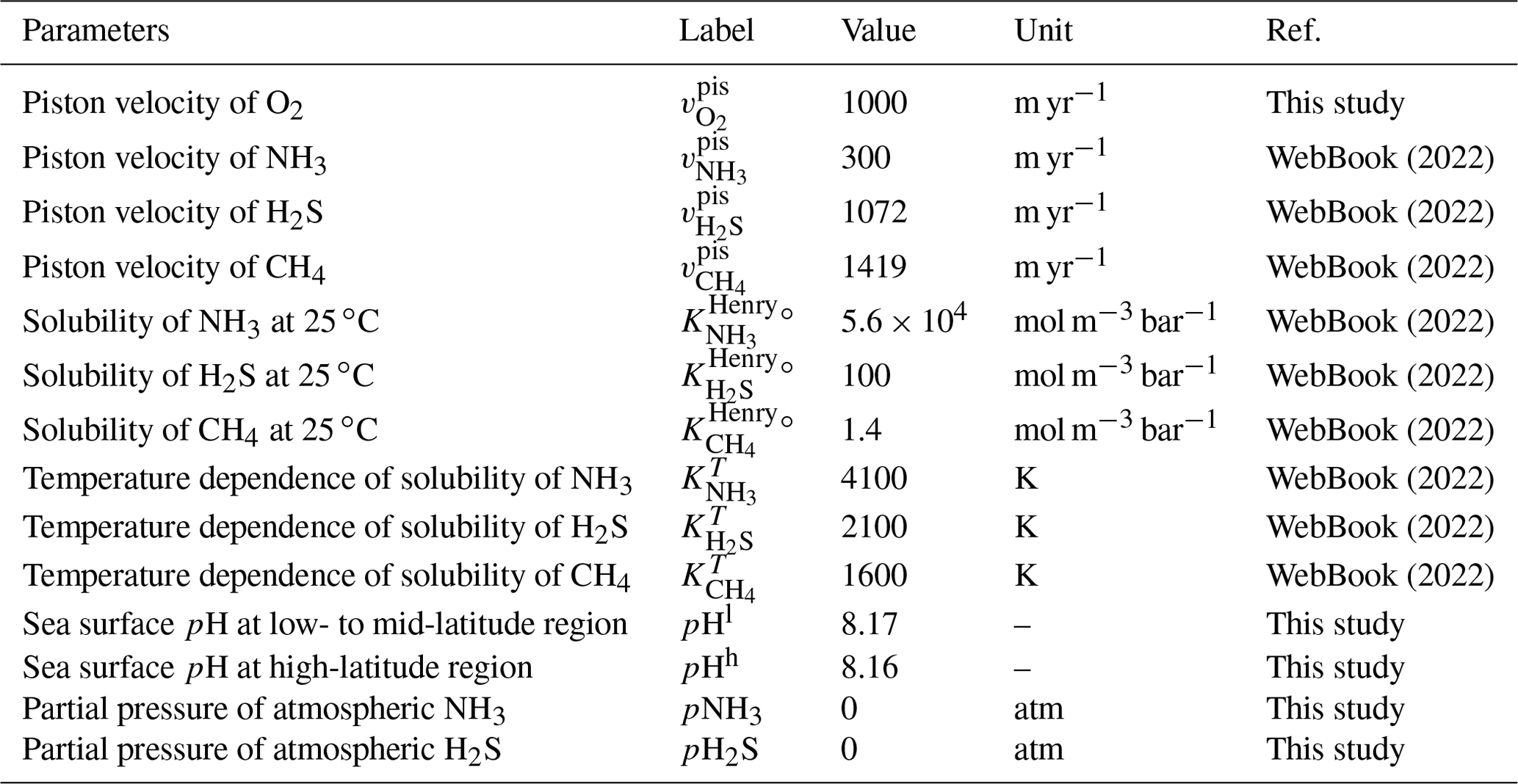
2.5 Land model

2.5.1 Net primary productivity

Terrestrial NPP is scaled by global land biomass V normalized to the modern value:

$$\begin{array}{}\text{(80)}& J_{\mathrm{NPP}}^{\mathrm{lnd}}=V\times J_{\mathrm{NPP}}^{\mathrm{lnd},\ast },\end{array}$$

where the present value of terrestrial NPP is set at 60 Gt C yr⁻¹ (Prentice et al., 2001). The global land biomass is a function of atmospheric O₂ levels:

$$\begin{array}{}\text{(81)}& V=f_{\mathrm{UV}}{f}_{\mathrm{fire}}{f}_{{\mathrm{O}}_{\mathrm{2}}},\end{array}$$

where $f_{{\mathrm{O}}_{\mathrm{2}}}$ represents the direct effect of atmospheric O₂ concentration on the C₃ plant growth and f_fire denotes the effect of fires on land biota (Bergman et al., 2004; Lenton and Watson, 2000b):

$$\begin{array}{}\text{(82)}& {\displaystyle }{f}_{{\mathrm{O}}_{\mathrm{2}}}=max\left\{\mathrm{1.5}-\mathrm{0.5}p{\mathrm{O}}_{\mathrm{2}}^{\mathrm{PAL}},\mathrm{0}\right\},\text{(83)}& {\displaystyle }{f}_{\mathrm{fire}}={\displaystyle \frac{k_{\mathrm{fire}}}{k_{\mathrm{fire}}-\mathrm{1}+\text{ignit}}}.\end{array}$$

Here k_fire (=3; Lenton, 2013) is the fire frequency constant and “ignit” is an ignition factor representing the fire frequency as a function of oxygen (Lenton, 2013; Lenton et al., 2018; Lenton and Watson, 2000b):

$$\begin{array}{}\text{(84)}& \text{ignit}=min\left\{max\left\{c_{\mathrm{1}}p{\mathrm{O}}_{\mathrm{2}}-c_{\mathrm{2}},\mathrm{0}\right\},c_{\mathrm{3}}\right\},\end{array}$$

with c₁=48, c₂=9.08, and c₃=5 (Lenton, 2013). CANOPS-GRB also includes an additional factor f_UV representing the effect of UV on the terrestrial biosphere as a function of atmospheric O₂ levels (Ozaki and Reinhard, 2021):

$$\begin{array}{}\text{(85)}& f_{\mathrm{UV}}=\tanh \left({\displaystyle \frac{p{\mathrm{O}}_{\mathrm{2}}^{\mathrm{PAL}}}{c_{\mathrm{UV}}}}\right),\end{array}$$

where c_UV is a model parameter, which in our standard model is set at 1 % PAL, meaning that terrestrial plant activity is suppressed when atmospheric O₂ is lower than a few % PAL.

2.5.2 Terrestrial biogeochemical cycles

Phosphorus weathering flux, $J_P^{\mathrm{w}}$ (Eq. 2), is treated as a boundary condition. A fraction of weathered P is ultimately buried as terrigenous organic matter (Eq. 3), whereas the remaining fraction is delivered to the ocean via rivers (Eq. 4). In the CANOPS-GRB model, the reference value of $J_{\mathrm{P}}^{\mathrm{r}}$ (=0.155 Tmol P yr⁻¹) is tuned so that the oceanic P level of the reference state is consistent with modern observations. The burial rate of terrigenous organic matter (in terms of C) can be written as follows:

$$\begin{array}{}\text{(86)}& J_{\mathrm{org}}^{\mathrm{b},\mathrm{lnd}}={\left({\mathrm{C}}_{\mathrm{org}}/{\mathrm{P}}_{\mathrm{org}}\right)}^{\mathrm{lnd}}{J}_{\mathrm{P}}^{\mathrm{b},\mathrm{lnd}},\end{array}$$

where (C_org $/$ P_org)^lnd (=1000) is the average $\mathrm{C}/\mathrm{P}$ burial ratio of terrigenous organic matter (Bergman et al., 2004). In this study, the reference value of $J_{\mathrm{org}}^{\mathrm{b},\mathrm{lnd}}$ was set at 3 Tmol C yr⁻¹. By combining Eqs. (3), (4), and (86) for the reference state, the proportional coefficient k₁₁ of Eq. (3) is determined by the reference state as follows:

$$\begin{array}{}\text{(87)}& k_{\mathrm{11}}={\displaystyle \frac{J_{\mathrm{org}}^{\mathrm{b},\mathrm{lnd},\ast }}{J_{\mathrm{org}}^{\mathrm{b},\mathrm{lnd},\ast }+{\left({\mathrm{C}}_{\mathrm{org}}/{\mathrm{P}}_{\mathrm{org}}\right)}^{\mathrm{lnd}}{J}_{\mathrm{P}}^{\mathrm{r},\ast }}}=\mathrm{0.0189}.\end{array}$$

The value of k₁₁ is treated as a constant in this study.

Almost all organic matter produced by terrestrial NPP is decomposed before burial. The total decomposition rate is given by

$$\begin{array}{}\text{(88)}& J_{\mathrm{org}}^{\mathrm{r},\mathrm{lnd}}=J_{\mathrm{NPP}}^{\mathrm{lnd}}-J_{\mathrm{org}}^{\mathrm{b},\mathrm{lnd}}.\end{array}$$

CANOPS-GRB includes aerobic respiration and methanogenesis as respiration pathways for terrigenous matter, and the CH₄ flux from the terrestrial ecosystem to the atmosphere is evaluated with the assumption that it is proportional to the burial rate of terrigenous organic matter:

$$\begin{array}{}\text{(89)}& J_{{\mathrm{CH}}_{\mathrm{4}}}^{\mathrm{lnd}}=\left({\displaystyle \frac{J_{\mathrm{org}}^{\mathrm{b},\mathrm{lnd}}}{J_{\mathrm{org}}^{\mathrm{b},\mathrm{lnd},\ast }}}\right)J_{{\mathrm{CH}}_{\mathrm{4}}}^{\mathrm{lnd},\ast },\end{array}$$

where the reference value was set at 1 Tmol CH₄ yr⁻¹. The net flux of CO₂, O₂ and CH₄ from the terrestrial ecosystem to the atmosphere can be written as follows:

$$\begin{array}{}\text{(90)}& {\displaystyle }{J}_{{\mathrm{CO}}_{\mathrm{2}}}^{\mathrm{lnd}}=\left(g_{{\mathrm{O}}_{\mathrm{2}}}+{\displaystyle \frac{\mathrm{1}}{\mathrm{2}}}\left(\mathrm{1}+\mathit{\delta }\right)g_{{\mathrm{CH}}_{\mathrm{4}}}\right)J_{\mathrm{org}}^{\mathrm{r},\mathrm{lnd}},\text{(91)}& {\displaystyle }{J}_{{\mathrm{O}}_{\mathrm{2}}}^{\mathrm{lnd}}=J_{\mathrm{NPP}}^{\mathrm{lnd}}-\left(g_{{\mathrm{O}}_{\mathrm{2}}}+\mathit{\delta }{g}_{{\mathrm{CH}}_{\mathrm{4}}}\right)J_{\mathrm{org}}^{\mathrm{r},\mathrm{lnd}},\text{(92)}& {\displaystyle }{J}_{{\mathrm{CH}}_{\mathrm{4}}}^{\mathrm{lnd}}={\displaystyle \frac{\mathrm{1}}{\mathrm{2}}}\left(\mathrm{1}-\mathit{\delta }\right)g_{{\mathrm{CH}}_{\mathrm{4}}}{J}_{\mathrm{org}}^{\mathrm{r},\mathrm{lnd}},\end{array}$$

where $g_{{\mathrm{O}}_{\mathrm{2}}}$ and $g_{{\mathrm{CH}}_{\mathrm{4}}}$ denote the fraction of organic matter decomposed by aerobic respiration and methanogenesis, respectively. δ represents the fraction of methane that is consumed by aerobic methanotrophy that is a function of O₂:

$$\begin{array}{}\text{(93)}& \mathit{\delta }={\displaystyle \frac{M_{{\mathrm{O}}_{\mathrm{2}}}^{\mathrm{atm}}}{M_{{\mathrm{O}}_{\mathrm{2}}}^{\mathrm{atm}}+K_{{\mathrm{O}}_{\mathrm{2}}}^{\prime }}},\end{array}$$

where $K_{{\mathrm{O}}_{\mathrm{2}}}^{\prime }=\mathrm{0.273}\times {\mathrm{10}}^{\mathrm{18}}$ mol (Goldblatt et al., 2006). A fraction of organic matter decomposed by methanogenesis, $g_{{\mathrm{CH}}_{\mathrm{4}}}$, can be calculated based on Eqs. (89) and (92). Following this, $g_{{\mathrm{O}}_{\mathrm{2}}}$ is determined from $\mathrm{1}-g_{{\mathrm{CH}}_{\mathrm{4}}}$.

2.5.3 Weathering

The oxidative weathering of continental crust is a major oxygen sink on geologic timescales, providing a fundamental control on atmospheric O₂ levels. The weathering rate in the model is assumed to be proportional to sedimentary reservoir size and a global erosion factor, f_R, expressing the effect of continental denudation and erosion on terrestrial weathering:

$$\begin{array}{}\text{(94)}& {\displaystyle }{J}_{\mathrm{org}}^{\mathrm{w}}=f_{\mathrm{R}}{f}_{\mathrm{orgw}}^{{\mathrm{O}}_{\mathrm{2}}}\left({\displaystyle \frac{\text{ORG}}{{\text{ORG}}^{\ast }}}\right)J_{\mathrm{org}}^{\mathrm{w},\ast },\text{(95)}& {\displaystyle }{J}_{\mathrm{pyr}}^{\mathrm{w}}=f_{\mathrm{R}}{f}_{\mathrm{pyrw}}^{{\mathrm{O}}_{\mathrm{2}}}\left({\displaystyle \frac{\text{PYR}}{{\text{PYR}}^{\ast }}}\right)J_{\mathrm{pyr}}^{\mathrm{w}\ast },\end{array}$$

where $J_{\mathrm{org}}^{\mathrm{w}}$ and $J_{\mathrm{pyr}}^{\mathrm{w}}$ denote the oxidative weathering of organic carbon and pyrite, respectively, and $f_{\mathrm{orgw}}^{{\mathrm{O}}_{\mathrm{2}}}$ and $f_{\mathrm{pyrw}}^{{\mathrm{O}}_{\mathrm{2}}}$ represent the O₂ dependency. For the oxidative weathering of organic matter, previous biogeochemical models have adapted a (pO${}_{\mathrm{2}}^{\mathrm{PAL}}{)}^{\mathrm{0.5}}$ relationship (Bergman et al., 2004; Lasaga and Ohmoto, 2002). In this study, we employ alternative empirical relationships based on results obtained from a 1-D weathering model (Bolton et al., 2006; Daines et al., 2017):

$$\begin{array}{}\text{(96)}& {\displaystyle }{f}_{\mathrm{orgw}}^{{\mathrm{O}}_{\mathrm{2}}}=c_{\mathrm{orgw}}{\displaystyle \frac{p{\mathrm{O}}_{\mathrm{2}}^{\mathrm{PAL}}}{p{\mathrm{O}}_{\mathrm{2}}^{\mathrm{PAL}}+K_{\mathrm{orgw}}}},\text{(97)}& {\displaystyle }{f}_{\mathrm{pyrw}}^{{\mathrm{O}}_{\mathrm{2}}}=c_{\mathrm{pyrw}}{\displaystyle \frac{p{\mathrm{O}}_{\mathrm{2}}^{\mathrm{PAL}}}{p{\mathrm{O}}_{\mathrm{2}}^{\mathrm{PAL}}+K_{\mathrm{pyrw}}}},\end{array}$$

where K_orgw and K_pyrw denote half-saturation constants (K_orgw=0.334 and K_pyrw=0.017) and c_orgw and c_pyrw are normalized constants (c_orgw=1.334 and c_pyrw=1.017), respectively. The Monod-type relationship captures the fact that the rate of oxidative weathering reaches its maximum as determined by the erosion rate under highly oxygenated conditions (i.e., transport-limited regime). For example, due to the fast dissolution kinetics of pyrite, oxidative weathering can be regarded as transport-limited under modern conditions (Bolton et al., 2006) (Fig. 10). In the CANOPS-GRB model, $J_{\mathrm{org}}^{\mathrm{w}\ast }$ is calibrated based on the global redox budget of the reference run (see Sect. 2.3.5).

It is important to note that above equations ignore the possible importance of microbial activity and temperature on the rate of oxidative weathering (Petsch et al., 2001; Soulet et al., 2021). Both represent important topics for future research.

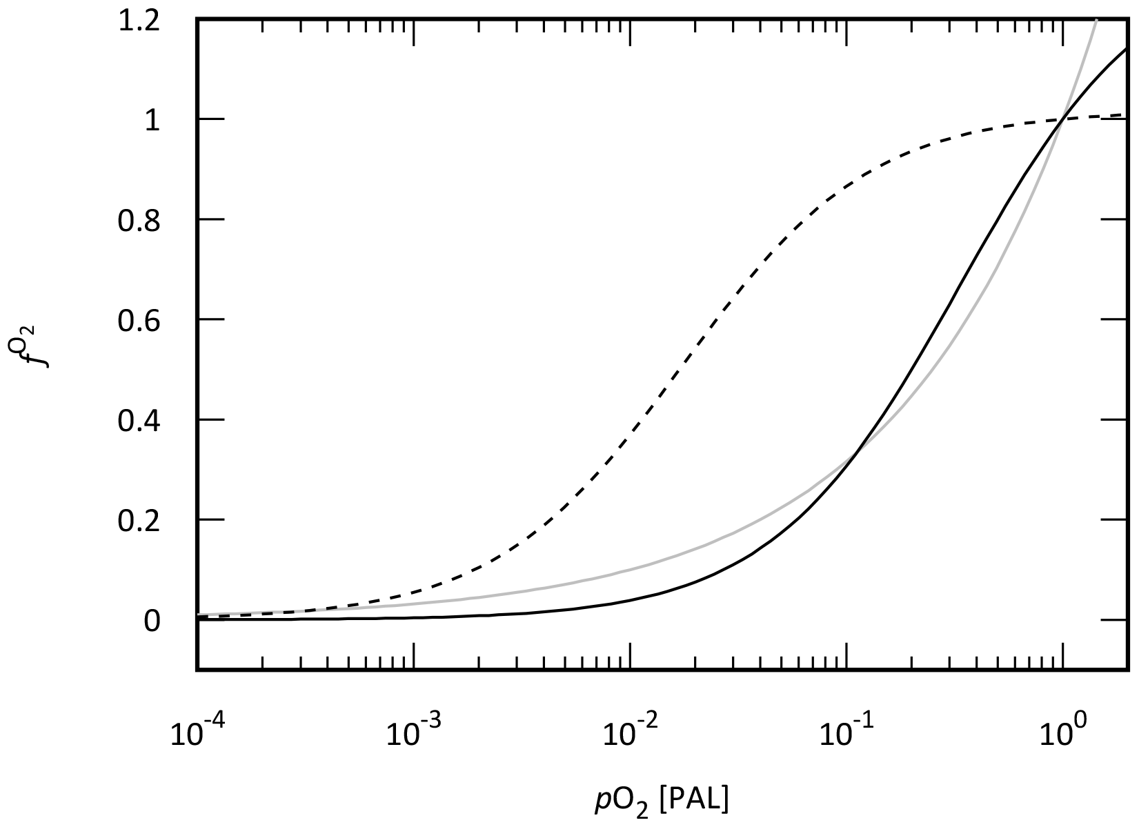
Figure 10 O₂ dependency of the oxidative weathering rate of organic matter and pyrite sulfur. The gray line denotes the (pO${}_{\mathrm{2}}^{\mathrm{PAL}}{)}^{\mathrm{0.5}}$ relationship assumed in previous biogeochemical models (Lasaga and Ohmoto, 2002; Daines et al., 2017). Solid and dashed black lines represent the empirical Monod-type relationships for oxidative weathering of organic matter (solid) and pyrite sulfur (dashed) based on the results obtained from a 1-D weathering model (Bolton et al., 2006; Daines et al., 2017), which are adopted in the standard model of the CANOPS-GRB model. PAL stands for present atmospheric level.

The present riverine flux of sulfur, $J_{\mathrm{S}}^{\mathrm{r}\ast }$, is estimated at 2.6 Tmol S yr⁻¹ (Raiswell and Canfield, 2012), representing the dominant source to the oceans. Riverine flux is written as the sum of the gypsum weathering flux $J_{\mathrm{gyp}}^{\mathrm{w}}$ and the oxidative weathering of pyrite $J_{\mathrm{pyr}}^{\mathrm{w}}$ and depends directly or indirectly on the oxidation state of the atmosphere:

$$\begin{array}{}\text{(98)}& J_{\mathrm{S}}^{\mathrm{r}}=J_{\mathrm{gyp}}^{\mathrm{w}}+J_{\mathrm{pyr}}^{\mathrm{w}}.\end{array}$$

Based on previous studies (Berner, 2009; Wortmann and Paytan, 2012; Bergman et al., 2004; Markovic et al., 2015), a 3 : 1 ratio in modern rivers of SO${}_{\mathrm{4}}^{\mathrm{2}-}$ from gypsum vs. pyrite weathering is assumed. Gypsum weathering flux is assumed to be proportional to its sedimentary reservoir size, GYP, and f_R:

$$\begin{array}{}\text{(99)}& J_{\mathrm{gyp}}^{\mathrm{w}}=f_{\mathrm{R}}\left({\displaystyle \frac{\text{GYP}}{{\text{GYP}}^{\ast }}}\right)J_{\mathrm{gyp}}^{\mathrm{w}\ast },\end{array}$$

where * represents the present value.

In the previous version of the CANOPS (Ozaki et al., 2019a), oxidative weathering of pyrite was divided into biogenic and abiotic weathering fluxes. In this study, we simplify this (Eq. 95). In addition, oxidative weathering of Fe(II)-bearing minerals is ignored in this study, which simplifies the framework of the global O₂ budget (Sect. 2.3.5).

2.5.4 Volcanic degassing

Volcanic outgassing fluxes of carbon and sulfur are assumed to be proportional to their respective crustal reservoir sizes:

$$\begin{array}{}\text{(100)}& {\displaystyle }{J}_{\mathrm{org}}^{\mathrm{m}}=\left({\displaystyle \frac{\text{ORG}}{{\text{ORG}}^{\ast }}}\right)J_{\mathrm{org}}^{\mathrm{m},\ast },\text{(101)}& {\displaystyle }{J}_{\mathrm{pyr}}^{\mathrm{m}}=\left({\displaystyle \frac{\text{PYR}}{{\text{PYR}}^{\ast }}}\right)J_{\mathrm{pyr}}^{\mathrm{m},\ast },\text{(102)}& {\displaystyle }{J}_{\mathrm{gyp}}^{\mathrm{m}}=\left({\displaystyle \frac{\text{GYP}}{{\text{GYP}}^{\ast }}}\right)J_{\mathrm{gyp}}^{\mathrm{m},\ast }.\end{array}$$

We set the reference value of the volcanic outgassing flux of organic carbon, $J_{\mathrm{org}}^{\mathrm{m},\ast }$, at 1.25 Tmol C yr⁻¹ (Bergman et al., 2004). The estimates of modern volcanic fluxes of sulfur fall within the range of ∼0.3–3 Tmol S yr⁻¹ (Kagoshima et al., 2015; Catling and Kasting, 2017; Raiswell and Canfield, 2012; Walker and Brimblecombe, 1985). We adopted a recent estimate of 0.8 Tmol S yr⁻¹ (Kagoshima et al., 2015).

2.5.5 Sedimentary reservoirs

We extend the original model framework to the explicit calculation of the secular evolution of the sedimentary reservoirs, linking the biogeochemical cycles in the ocean–atmosphere system to the rock cycle. The mass balance equation for sedimentary organic carbon (ORG) can be written as follows:

$$\begin{array}{}\text{(103)}& {\displaystyle \frac{\mathrm{d}\text{ORG}}{\mathrm{d}t}}=J_{\mathrm{org}}^{\mathrm{b}}-J_{\mathrm{org}}^{\mathrm{w}}-J_{\mathrm{org}}^{\mathrm{m}},\end{array}$$

where $J_{\mathrm{org}}^{\mathrm{b}}$ denotes the sum of the burial rate of marine and terrigenous organic matter ($J_{\mathrm{org}}^{\mathrm{b},\mathrm{ocn}}+J_{\mathrm{org}}^{\mathrm{b},\mathrm{lnd}}$), the primary source of sedimentary organic carbon. Primary outputs are oxidative weathering, volcanic outgassing, and metamorphism. Previous estimates of the present reservoir size of ORG fall in the range of 1000–1300 Emol (1 E = 10¹⁸) (Berner, 1989; Garrels and Perry, 1974; Mackenzie et al., 1993). We assumed 1250 Emol for the reference value of ORG.

The sedimentary reservoir sizes of pyrite sulfur (PYR) and gypsum sulfur (GYP) are also written as the balance between the input (burial) and outputs (weathering and outgassing):

$$\begin{array}{}\text{(104)}& {\displaystyle \frac{\mathrm{d}\text{PYR}}{\mathrm{d}t}}=J_{\mathrm{pyr}}^{\mathrm{b}}-J_{\mathrm{pyr}}^{\mathrm{w}}-J_{\mathrm{pyr}}^{\mathrm{m}},\text{(105)}& {\displaystyle \frac{\mathrm{d}\text{GYP}}{\mathrm{d}t}}=J_{\mathrm{gyp}}^{\mathrm{b}}-J_{\mathrm{gyp}}^{\mathrm{w}}-J_{\mathrm{gyp}}^{\mathrm{m}},\end{array}$$

where $J_{\mathrm{pyr}}^{\mathrm{b}}$ represents the sum of pyrite precipitation rates in the water column and sediments, $J_{\mathrm{pyr}}^{\mathrm{b},\mathrm{wc}}+J_{\mathrm{pyr}}^{\mathrm{b},\mathrm{sed}}$. Previous estimates of present reservoir sizes of GYP and PYR fall in the range of 77–300 Emol and 155–300 Emol (Berner, 2006; Bottrell and Newton, 2006; Yaroshevsky, 2006; Kump, 1989; Lasaga, 1989; Holser et al., 1989; Sleep, 2005; Schlesinger and Bernhardt, 2013), respectively. We adopted 200 and 200 Emol for GYP^∗ and PYR^∗.

2.6 Atmosphere model

2.6.1 Hydrogen escape

The rate of hydrogen escape is assumed to be diffusion limited as it is today. Thus, the total concentration of all H-bearing compounds in the lower stratosphere determines the rate of hydrogen escape (Walker, 1977). For Proterozoic-Phanerozoic atmospheres, CH₄ appears to have been the dominant hydrogen-bearing species in the stratosphere, and the flux, J_Hesc (mol yr⁻¹), is calculated as

$$\begin{array}{}\text{(106)}& J_{\mathrm{Hesc}}=s{M}_{{\mathrm{CH}}_{\mathrm{4}}}^{\mathrm{atm}},\end{array}$$

where $M_{{\mathrm{CH}}_{\mathrm{4}}}^{\mathrm{atm}}$ denotes the abundance of CH₄ in the atmosphere (mol) and s ($=\mathrm{3.7}\times {\mathrm{10}}^{-\mathrm{5}}$ yr⁻¹) is a proportional coefficient (Goldblatt et al., 2006).

2.6.2 Photochemistry

CANOPS-GRB includes parameterized O₂–O₃–CH₄ photochemistry that allows quantification of the abundances of atmospheric O₂ and CH₄. The rate of oxidation of CH₄ is calculated by the following empirical parameterization that was obtained from a 1-D photochemistry model (Claire et al., 2006):

$$\begin{array}{}\text{(107)}& J_{{\mathrm{CH}}_{\mathrm{4}}\mathrm{ox}}=k_{{\mathrm{CH}}_{\mathrm{4}}\mathrm{ox}}{M}_{{\mathrm{O}}_{\mathrm{2}}}^{\mathrm{atm}}{M}_{{\mathrm{CH}}_{\mathrm{4}}}^{\mathrm{atm}},\end{array}$$

where $M_{{\mathrm{O}}_{\mathrm{2}}}^{\mathrm{atm}}$ and $M_{{\mathrm{CH}}_{\mathrm{4}}}^{\mathrm{atm}}$ denote the abundance of O₂ and CH₄ in the atmosphere (mol). The reaction rate $k_{{\mathrm{CH}}_{\mathrm{4}}\mathrm{ox}}$ (mol⁻¹ yr⁻¹) is expressed as a polynomial function of the reservoir sizes of O₂ and CH₄ (Ozaki and Reinhard, 2021):

$$\begin{array}{}\text{(108)}& \begin{array}{rl}\log k_{{\mathrm{CH}}_{\mathrm{4}}\mathrm{ox}}& ={\mathit{\alpha }}_{\mathrm{0}}^j+{\mathit{\alpha }}_{\mathrm{1}}^j\cdot {\mathit{\phi }}_{{\mathrm{O}}_{\mathrm{2}}}+{\mathit{\alpha }}_{\mathrm{2}}^j\cdot {\mathit{\phi }}_{{\mathrm{O}}_{\mathrm{2}}}^{\mathrm{2}}+{\mathit{\alpha }}_{\mathrm{3}}^j\cdot {\mathit{\phi }}_{{\mathrm{O}}_{\mathrm{2}}}^{\mathrm{3}}\\ & +{\mathit{\alpha }}_{\mathrm{4}}^j\cdot {\mathit{\phi }}_{{\mathrm{O}}_{\mathrm{2}}}^{\mathrm{4}}+{\mathit{\alpha }}_{\mathrm{5}}^j\cdot {\mathit{\phi }}_{{\mathrm{O}}_{\mathrm{2}}}^{\mathrm{5}}+{\mathit{\alpha }}_{\mathrm{6}}^j\cdot {\mathit{\phi }}_{{\mathrm{O}}_{\mathrm{2}}}^{\mathrm{6}},\end{array}\end{array}$$

where $a_i^j$ represents fitting coefficients for given atmospheric CH₄ levels and ϕ_O2 is logpO₂ (in bar) (supplementary Table 4 of Ozaki and Reinhard, 2021). The oxidation rate was evaluated using Fig. 3 of Claire et al. (2006), showing the oxidation rate as a function of pO₂ and pCH₄. We took the relationship between $k_{{\mathrm{CH}}_{\mathrm{4}}\mathrm{ox}}$ and pO₂ for pCH₄ of 10⁻⁶, 10⁻⁵, 10⁻⁴, 10⁻³, and $\mathrm{2}\times {\mathrm{10}}^{-\mathrm{3}}$ bar, and $k_{{\mathrm{CH}}_{\mathrm{4}}\mathrm{ox}}$ is calculated as a function of pO₂ and pCH₄ with a log-linear interpolation method. Note that the default photochemical parameterization presented above limits the applicability of CANOPS-GRB v1.0 to Earth-like planets around the Sun-like host stars. Current work is focused on elaborating parameterized photochemistry across a wider range of spectral energy distributions.

2.6.3 Mass balance

CANOPS-GRB accounts for the atmospheric concentrations of O₂ and CH₄. The atmospheric concentration of O₂ is determined by the biogenic source (from the ocean and terrestrial ecosystems) and the consumption through the series of oxidation reaction (the continental weathering of kerogen and pyrite, volcanic outgassing, and photochemical oxidation of methane):

$$\begin{array}{}\text{(109)}& \begin{array}{rl}{\displaystyle \frac{\mathrm{d}{M}_{{\mathrm{O}}_{\mathrm{2}}}^{\mathrm{atm}}}{\mathrm{d}t}}& =J_{{\mathrm{O}}_{\mathrm{2}}\uparrow }^{\mathrm{air}-\mathrm{sea}}+J_{{\mathrm{O}}_{\mathrm{2}}\uparrow }^{\mathrm{air}-\mathrm{lnd}}-\left(J_{\mathrm{Hesc}}+\mathrm{2}{J}_{{\mathrm{CH}}_{\mathrm{4}}\text{ox}}\right)\\ & -\left(J_{\mathrm{org}}^{\mathrm{w}}+J_{\mathrm{org}}^{\mathrm{m}}\right)-\mathrm{2}\left(J_{\mathrm{pyr}}^{\mathrm{w}}+J_{\mathrm{pyr}}^{\mathrm{m}}\right),\end{array}\end{array}$$

where $M_{{\mathrm{O}}_{\mathrm{2}}}^{\mathrm{atm}}$ denotes the mass of O₂ in the atmosphere (moles) and the first and second term on the right-hand side represents the biogenic flux of O₂ from marine and terrestrial ecosystems. The third term denotes O₂ consumption via photochemistry, and the fourth and fifth terms are the O₂ consumption via organic C and pyrite S sub-cycles. Note that the hydrogen escape to space is represented as the O₂ sink because the hydrogen escape via CH₄ followed by the oxidation of carbon to CO₂ is represented as

$$\begin{array}{}\text{(110)}& {\mathrm{CH}}_{\mathrm{4}}+{\mathrm{O}}_{\mathrm{2}}+h\mathit{\nu }\to \mathrm{4}\mathrm{H}\uparrow +{\mathrm{CO}}_{\mathrm{2}}.\end{array}$$

On the other hand, the photochemical oxidation of CH₄ can be written as follows:

$$\begin{array}{}\text{(111)}& {\mathrm{CH}}_{\mathrm{4}}+\mathrm{2}{\mathrm{O}}_{\mathrm{2}}+h\mathit{\nu }\to \mathrm{2}{\mathrm{H}}_{\mathrm{2}}\mathrm{O}+{\mathrm{CO}}_{\mathrm{2}}.\end{array}$$

Thus, the hydrogen escape to space represents the net gain of oxidizing power to the system (see Eq. 12).

The abundance of CH₄ in the atmosphere, $M_{{\mathrm{CH}}_{\mathrm{4}}}^{\mathrm{atm}}$, is determined by input from the ecosystems and the consumption of CH₄ via photolysis, as well as by the hydrogen escape:

$$\begin{array}{}\text{(112)}& {\displaystyle \frac{\mathrm{d}{M}_{{\mathrm{CH}}_{\mathrm{4}}}^{\mathrm{atm}}}{\mathrm{d}t}}=J_{{\mathrm{CH}}_{\mathrm{4}}\uparrow }^{\mathrm{air}-\mathrm{sea}}+J_{{\mathrm{CH}}_{\mathrm{4}}\uparrow }^{\mathrm{air}-\mathrm{lnd}}-\left(J_{\mathrm{Hesc}}+J_{{\mathrm{CH}}_{\mathrm{4}}\mathrm{ox}}\right).\end{array}$$

No abiotic CH₄ input via hydrothermal systems is included.

3 Validation against the modern global ocean

Here, a steady-state simulation mimicking the present-day condition was run to evaluate the overall performance of CANOPS-GRB. To do this, the ocean model was run until reaching steady state, assuming the present atmospheric O₂ level and reference values of boundary fluxes (weathering and volcanic fluxes). The simulated circulation and biogeochemistry for the modern global ocean was compared with modern oceanographic observations from the Global Ocean Data Analysis Project (Key et al., 2015; Olsen et al., 2016).

3.1 Distribution of circulation tracers

Comparisons of model output with circulation tracers, such as potential temperature (θ) and radiocarbon (Δ¹⁴C), permit a test of the physical exchange scheme. Figure 11 depicts the simulated patterns of physical tracers with observational data. The physical circulation in the model generally agrees well with oceanic observations, although we note that model temperatures for low- to mid-latitudes above 1000 m water depth tend to be higher than observed because temperature distribution in the real ocean is strongly controlled by vertical structure and advective processes that are not captured in our simple circulation scheme. Despite this model limitation, the modeled temperature distribution generally reproduces the observed distribution. The Δ¹⁴C minimum in the model for the low- to mid-latitude region corresponds well with observations. The modeled background radiocarbon for young deep waters (about $-\mathrm{150}\pm \mathrm{25}$ ‰) is closer to the value for the Southern Ocean (approximately −150 ‰) than for North Atlantic deep waters (approximately −80 ‰), and old deep waters ($-\mathrm{200}\pm \mathrm{15}$ ‰) correspond to the South Pacific. We conclude that the simulated circulation tracers generally match well with ocean data.

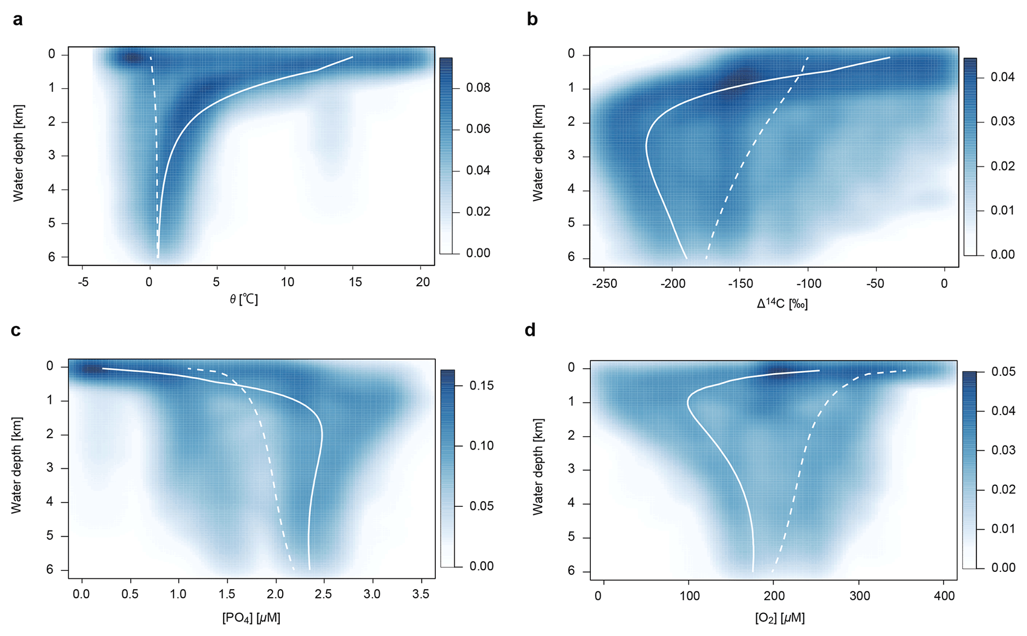
Figure 11 Simulated steady-state depth profiles of (a) potential temperature, θ, (b) radiocarbon, Δ¹⁴C, (c) DIP (dissolved inorganic phosphorus, PO${}_{\mathrm{4}}^{\mathrm{3}-}$), and (d) dissolved oxygen, O₂. Solid and dashed white lines denote the simulated profiles for the LD and HD regions, respectively. Simulation results are compared with the dataset from the Global Ocean Data Analysis Project (GLODAP) database (GLODAPv2_2019; Key et al., 2015; Olsen et al., 2016). The color represents the density of observational points.

3.2 Ocean biogeochemistry

Having demonstrated that CANOPS-GRB's ocean circulation model does a reasonable job of representing water mass exchange, we next assess the performance of the oceanic biogeochemistry model by comparing its output to ocean biogeochemical data. Model-generated global fluxes and inventories of C, P, N and S cycles are summarized in Fig. 12. These compare well with independent observational estimates. Below, we provide a brief discussion of globally integrated biogeochemical flux estimates.

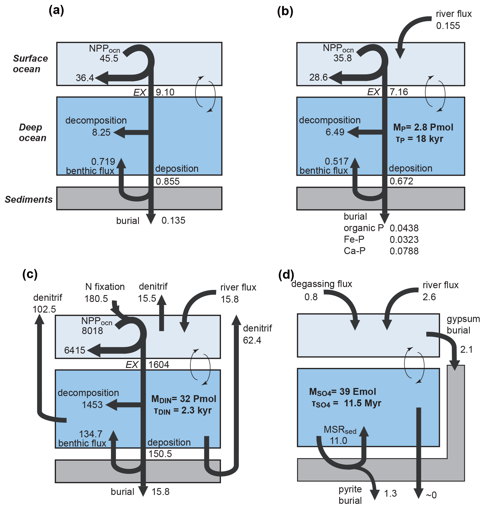
Figure 12 Schematics of the simulated material flow in the ocean for the reference run. (a) Organic carbon (in Gt C yr⁻¹), (b) phosphorus (in Tmol P yr⁻¹), (c) nitrogen (in Tg N yr⁻¹), and (d) sulfur (in Tmol S yr⁻¹). NPP_ocn is oceanic net primary production. EX represents export production. M_X is the mass of X in the ocean. τ_X is the residence time of X in the ocean. Pmol stands for 10¹⁵ mol, and Emol stands for 10¹⁸ mol.

3.2.1 Distribution of nutrients and oxygen

The simulated vertical profile of phosphate captures the characteristic features and values of observational data (Fig. 11c). More specifically, the distribution in the low- to mid-latitude region is more similar to that in the Pacific and Indian oceans, and distribution in the high- to mid-latitude region is similar to that in the Southern Ocean. This is a consequence of limiting high-latitude productivity (preformed DIP is 1.1 µM) which results in higher concentrations in the ocean interior. The model dissolved O₂ profile for low- to mid-latitude areas shows a minimum of approximately 100 µM at water depth of 1000 m, corresponding to the oxygen minimum zone (Fig. 11d). In contrast, dissolved O₂ for the high- to mid-latitude sector (HD) shows a monotonically decreasing trend. This is because of oxygen consumption via POM decomposition during downwelling.

3.2.2 Carbon cycling

The marine export and new production in our model is 9.1 Gt C yr⁻¹ (8.36 Gt C yr⁻¹ at L and 0.74 Gt C yr⁻¹ at H). This is consistent with previously estimated global values of 8.5–12 Gt C yr⁻¹ (Dunne et al., 2007; Laws et al., 2000; Sarmiento and Gruber, 2006; Heinze et al., 2009). In particular, our estimate is close to the mid-point of the previously estimated range of 9.6±3.6 Gt C yr⁻¹ (Dunne et al., 2007). This is a marked improvement from earlier studies with box models that have underestimated marine new production by a factor of 2 or more (Archer et al., 2000; Shaffer et al., 2008). Simulated global oceanic NPP is 45.5 Gt C yr⁻¹. This is also consistent with the previous estimated range of 44–65 Gt C yr⁻¹ (Prentice et al., 2001; Woodward, 2007; Carr et al., 2006; Berelson et al., 2007).

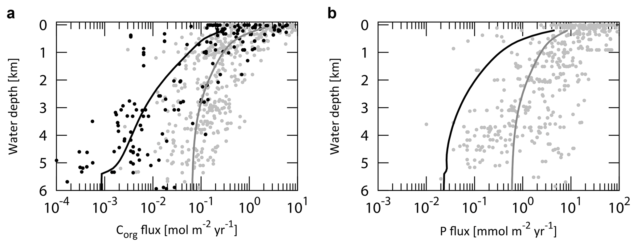
Figure 13 Simulated steady-state depth profiles of organic C and reactive P flux density for the LD region. In (a), gray dots denote observations of depositional/settling flux density, whereas black dots represent observations of burial flux density compiled from literature survey (Baturin, 2007; Betts and Holland, 1991; Colman and Holland, 2000; Lutz et al., 2002). Solid gray and black lines denote the simulated POC depositional and burial flux densities obtained from the reference run. (b) Gray dots denote the benthic P efflux density obtained from literature survey (Hartnett and Devol, 2003; Hensen et al., 1998; Ingall and Jahnke, 1994, 1997; McManus et al., 1997; Colman and Holland, 2000; Schenau and De Lange, 2001; Zabel et al., 1998), whereas solid gray and black lines represent the simulated benthic P efflux density and burial flux density of reactive P obtained from the reference run. The burial flux density of reactive P is not shown due to the sparseness of such observations.

The global marine POC flux depends largely on water depth. Model-generated fluxes compare well with independent estimates of deposition, burial, and regeneration. The gray line in Fig. 13a shows the simulated sinking flux density of POC in the water column for LD region, compared with observations (Archer et al., 2002; Betts and Holland, 1991; Lutz et al., 2002; Baturin, 2007). The preferential consumption of labile compounds (G₁ and G₂) during the settling process leads to a continuous decrease in reactivity and therefore remineralization rates from the surface ocean down to the deep. Our estimate lies well within the range of observations. The model tends to give lower fluxes than observed above 2000 m water depth and higher below 5000 m water depth. This is probably because of the assumption of homogeneous productivity in the surface ocean. In the real ocean, oceanic productivity is generally greater at the continental margins than in the pelagic gyre regions (Lutz et al., 2002). This is a model limitation, but the simulated biological pump is sufficient to describe the general characteristics of global ocean biogeochemistry.

Of total exported POC, 91 % (8.25 Gt C yr⁻¹) is decomposed in the water column and the rest (0.85 Gt C yr⁻¹) sinks to the sediment surface (Fig. 12a). The simulated global POC depositional flux is comparable not only with observational estimates of 0.93 Gt C yr⁻¹ (Muller-Karger et al., 2005) and 0.67±0.48 Gt C yr⁻¹ for off-shore regions (Dunne et al., 2007) but also with an estimate using EMIC (0.87 Gt C yr⁻¹) (Ridgwell and Hargreaves, 2007). The depositional fluxes of C_org in marginal (<2000 m) and deep-sea sediments (>2000 m) are estimated at 0.58 and 0.27 Gt C yr⁻¹, respectively. These estimates are slightly lower than previous estimates of 0.62–1.98 and 0.31–0.62 Gt C yr⁻¹ (Bohlen et al., 2012; Dunne et al., 2007; Muller-Karger et al., 2005; Burdige, 2007).

In our standard run, benthic remineralization removes 7.9 % of the exported POC (0.72 Gt C yr⁻¹), equivalent of 84 % of the global POC sedimentation rate. As a result, only 1.5 % (0.135 Gt C yr⁻¹ or 11.3 Tmol C yr⁻¹) of the global POC export production is ultimately buried in marine sediments. Our model demonstrates that much (91 %) of the total burial occurs on the continental margins (<2000 m water depth), where the settling flux and burial efficiency are relatively high. Previous studies (Dunne et al., 2007; Muller-Karger et al., 2005) estimated a C_org burial rate of 0.29±0.15 and $>\mathrm{0.06}\pm \mathrm{0.06}$ Gt C yr⁻¹ at the margin. Our estimate of 0.123 Gt C yr⁻¹ lies between these values, whereas our estimate for the deep sea, 0.012 Gt C yr⁻¹, is on the lower end of previous estimates of 0.012±0.02 Gt C yr⁻¹ (Dunne et al., 2007) and 0.017±0.005 Gt C yr⁻¹ (Hayes et al., 2021). In addition, Sarmiento and Gruber (2006) and Hayes et al. (2021) estimated the burial rate below 1000 m as 0.02±0.006 Gt C yr⁻¹; our estimate of 0.019 Gt C yr⁻¹ is consistent with this. Combined with the prescribed burial rate of terrigenous C_org 0.036 Gt C yr⁻¹ (3 Tmol C yr⁻¹), the total burial rate is calculated to be 0.17 Gt C yr⁻¹ (14.3 Tmol C yr⁻¹). This is somewhat higher than previous estimates (Berner, 1982; Burdige, 2005; Muller-Karger et al., 2005), but given the rather large uncertainty we consider it defensible.

Figure 14 shows OPD as a function of water depth. Although the benthic data could be biased towards highly specific environments, such as sediments underlying upwelling areas and continental margins, our estimates capture the general features of modern observations.

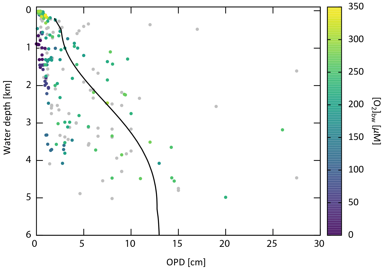
Figure 14 Oxygen penetration depth (OPD) as a function of water depth. Colored dots denote the observational data obtained from literature survey (Bradley et al., 2020; Donis et al., 2016; Nierop et al., 2017; Rowe et al., 2008; McManus et al., 2005; Martin and Sayles, 2014; Pfeifer et al., 2002; Hyacinthe et al., 2001; Hartnett et al., 1998; Hedges et al., 1999; Morford and Emerson, 1999; Devol and Christensen, 1993; Gundersen and Jorgensen, 1990; Sachs et al., 2009). The color represents the O₂ concentration of bottom water, [O₂]_bw, with gray dots for the unknown [O₂]_bw value. The simulated OPD obtained from the reference run is shown as a black line.

3.2.3 Phosphorus cycling

The removal of phosphate from surface waters occurs through photosynthetic fixation by primary producers and subsequent export in the form of POP into deeper waters, where it is largely remineralized back into DIP. Through this process there is a vertical partitioning of DIP within the ocean with reduced surface concentrations. Phosphorus export production is 7.16 Tmol P yr⁻¹, which is coupled with carbon according to the POM compositional ratio (C:P = 106:1 for our standard model). The remineralization in the water column (6.49 Tmol P yr⁻¹) and total sedimentation rate (0.672 Tmol P yr⁻¹) are also proportional to those of POC. In contrast, the benthic DIP flux is decoupled from the carbon flux. Figure 13b shows modeled DIP benthic efflux and burial flux together with observed fluxes. Some observational data showing a relatively large abyssal (4–6 km) benthic flux are from upwelling regions in the South Atlantic (Hensen et al., 1998). The deviation is therefore not critical for our globally averaged model. Our model gives the total benthic efflux of DIP as 0.517 Tmol P yr⁻¹, which is roughly three times the riverine reactive P input rate. This is within the range of previous estimates of 0.05–1.25 Tmol P yr⁻¹ (Wallmann, 2003, 2010; Compton et al., 2000; Colman and Holland, 2000).

The preservation efficiency (here defined as burial flux divided by the export flux) of P is 2.1 %. This is higher than that of organic carbon (1.5 %), indicating that more P is trapped in marine sediments than might be expected from Redfield stoichiometry. In marine sediments overlain by oxic bottom waters, a fraction of the DIP released to pore waters from POM decomposition can be absorbed by iron oxyhydroxide or precipitated as authigenic fluorapatite (Fig. 9). Therefore, the global averaged ${\mathrm{C}}_{\mathrm{org}}/{\mathrm{P}}_{\mathrm{reac}}$ ratio of buried sediments is generally less than the Redfield of 106 (approximately 65±25 based on observations; Algeo and Ingall, 2007). The modeled global average ${\mathrm{C}}_{\mathrm{org}}/{\mathrm{P}}_{\mathrm{reac}}$ ratio of buried sediment is 73, which is consistent with this. The P burial fluxes of organic P, Fe-bound P, and authigenic P are estimated at 0.044, 0.032, and 0.079 Tmol P yr⁻¹, respectively.

The ${\mathrm{C}}_{\mathrm{org}}/{\mathrm{P}}_{\mathrm{org}}$ ratio of burying organic matter shows a nonlinear relationship with respect to sedimentation rate. The observed ${\mathrm{C}}_{\mathrm{org}}/{\mathrm{P}}_{\mathrm{org}}$ ratios are generally greater than the Redfield value of 106, especially for sediments in oxygen minimum zones (OMZs), which are characterized by a high depositional flux of organic matter (${\mathrm{C}}_{\mathrm{org}}/{\mathrm{P}}_{\mathrm{org}}$ ratios up to 600 for the present open ocean) (Ingall and Cappellen, 1990). For example, the averaged ${\mathrm{C}}_{\mathrm{org}}/{\mathrm{P}}_{\mathrm{org}}$ molar ratio at the Peru–Chile OMZ and Black Sea are 600, and the estimated burial ratio of sapropel S1 of Mediterranean Sea is in the range of 400–800 (Slomp et al., 2002). This reflects the preferential regeneration of P relative to C during microbial remineralization of marine organic matter and reflects the more labile nature of P biochemicals relative to most non-phosphorus-containing organic carbon compounds. Additional rationale for this observation is that P is preferentially targeted for remineralization to support subsequent biological productivity as an essential and potentially limiting nutrient. Our model demonstrates that we can reproduce the first-order relationship between ${\mathrm{C}}_{\mathrm{org}}/{\mathrm{P}}_{\mathrm{org}}$ and sediment accumulation rate (Fig. 15).

The modeled marine DIP inventory is 2.75×10¹⁵ mol, consistent with the observational estimate of around 3×10¹⁵ mol (e.g., Delaney, 1998; Guidry et al., 2000). Given the riverine reactive P input flux of 0.155 Tmol P yr⁻¹, the phosphorus residence time is estimated at 18 kyr, which is also consistent with previous estimates of 20 kyr or shorter (Benitez-Nelson, 2000; Ruttenberg, 2003).

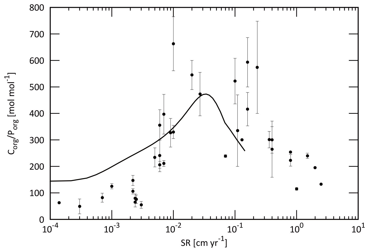
Figure 15 ${\mathrm{C}}_{\mathrm{org}}/{\mathrm{P}}_{\mathrm{org}}$ ratios of buried sediments as a function of sedimentation rate. Black dots represent the observational data (Ingall and Cappellen, 1990). The simulated ${\mathrm{C}}_{\mathrm{org}}/{\mathrm{P}}_{\mathrm{org}}$ ratios for the LD region obtained from our reference run is shown as a black line.

3.2.4 Nitrogen cycling

Nitrogen export production is 1603 Tg N yr⁻¹, which is coupled with carbon according to the C:N stoichiometry of organic matter. Simulated N fixation required for the N balance in the ocean is 180 Tg N yr⁻¹, which is higher than the range of previous estimates of 110–150 Tg N yr⁻¹ (Luo et al., 2012; Gruber and Sarmiento, 1997; Galloway et al., 2004; Karl et al., 2002; Fowler et al., 2013; Duce et al., 2008; Deutsch et al., 2007), while a recent study (Großkopf et al., 2012) suggests a higher value of ∼180 Tg N yr⁻¹. This discrepancy is partly because atmospheric deposition is ignored in the CANOPS-GRB model, which contributes 25.8 Tg N yr⁻¹ (Wang et al., 2019). Gruber and Sarmiento (2002) estimated the preindustrial value of the total source of N as 188±44 Tg N yr⁻¹. Our estimate of 196 Tg N yr⁻¹ is within this range.

Nitrogen fluxes in an oxic water column are tightly coupled with the C_org fluxes, whereas decoupling appears in suboxic environments. Simulated denitrification in the water column is 102 Tg N yr⁻¹, within the range of the observational estimates (50–150 Tg N yr⁻¹) (DeVries et al., 2012, 2013; Brandes and Devol, 2002; Gruber, 2008; Gruber and Sarmiento, 2002; Oschlies et al., 2008; Wang et al., 2019). Modeled benthic denitrification is 62 Tg N yr⁻¹, which is lower than the estimated range of 90–300 Tg N yr⁻¹ (DeVries et al., 2012, 2013; Brandes and Devol, 2002; Eugster and Gruber, 2012; Devol, 2015; Wang et al., 2019) by a factor of 1.5–5, suggesting that further efforts are required to improve representation of this process. One possible explanation for this discrepancy is that our model is not sufficient to express benthic N cycling because we ignore localized upwelling regions (such as the eastern Tropical Pacific and the Arabian Sea) and coastal regions where benthic denitrification is significant POM decomposition pathway in favor of globally averaged parameterizations. The separate treatment of continental shelves and margin sediments from the pelagic ocean could improve this issue. We also ignore another denitrification mechanism: anaerobic ammonium oxidation (anammox), which will often play an important role in the loss of fixed nitrogen in marine sediments and pelagic anoxic zones (Karthäuser et al., 2021; Kuypers et al., 2005).

The modeled DIN inventory is 4.5×10⁵ Tg N. Given the total source flux of 196 Tg N yr⁻¹, the residence time of DIN is estimated at 2.3 kyr.

3.2.5 Sulfur cycling

MSR is a major early diagenetic pathway of carbon oxidation in organic-rich sediments deposited below oxygenated waters. For the standard run, aerobic oxidation is a dominant process in the water column, but MSR contributes 37 % of benthic degradation. CANOPS-GRB estimates a global rate of benthic sulfate reduction at 11 Tmol S yr⁻¹. This is lower than the previously reported value of gross MSR (40–75 Tmol S yr⁻¹; Canfield and Farquhar, 2009; Jørgensen and Kasten, 2006) but agrees better with net MSR (Bowles et al., 2014). Bowles et al. (2014) have estimated global net MSR at 6.2 and 11.3 Tmol S yr⁻¹ for z>200 m depth and z>0 m depth, respectively. Our estimate is within this range. MSR is most pronounced on the shelf where high fluxes of organic matter to the seafloor lead to shallow OPD, high sulfide production, and consequently high pyrite precipitation (Fig. 16).

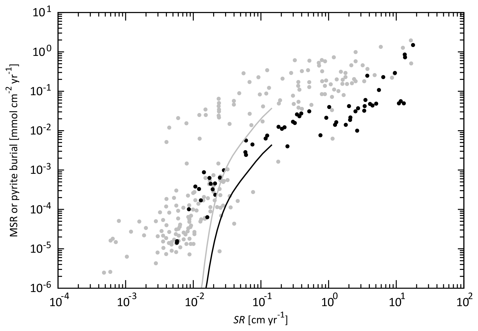
Figure 16 MSR and pyrite burial flux density as a function of sedimentation rate. Gray and black dots depict observational data compilation of depth-integrated MSR flux density and pyrite burial flux density for normal (oxic) marine sediments (Berner and Canfield, 1989; Canfield, 1989; Raiswell and Canfield, 2012). The unit of sedimentation rate was converted from g cm⁻² yr⁻¹ to cm yr⁻¹, assuming a dry bulk density of 2.5 g cm⁻³ and porosity of 0.9. Solid lines are the results obtained from the reference run of the CANOPS-GRB model.

In the CANOPS-GRB model, pyrite burial efficiency e_pyr (Sect. 2.4.4) for sediments underlying oxic bottom waters is set such that simulated seawater [SO${}_{\mathrm{4}}^{\mathrm{2}-}$] of the reference run is consistent with the modern value of 28.9 mM. The tuned value of 11.7 % agrees well with observations suggesting that pyrite precipitation rate is about 10 %–20 % of the rate of MSR (Fig. 16). Our reference value is also consistent with other estimates of 11 %–20 % (Bottrell and Newton, 2006; Tarhan et al., 2015; Turchyn and Schrag, 2006).

The sulfate inventory of our reference state is 39×10¹⁸ mol. Given the total source flux of 3.4 Tmol S yr⁻¹, the residence time of sulfate is 11.5 Myr.

3.3 Global oxygen cycling

The global O₂ budget for our reference state is shown in Fig. 17. The simulated O₂ inventory in the ocean-atmosphere system is 38×10¹⁸ mol (atmosphere = 38×10¹⁸ mol, ocean = 0.23×10¹⁸ mol). Organic carbon burial represents a major O₂ source flux (marine = 11.3 Tmol O₂ equiv. yr⁻¹ and terrigenous = 3 Tmol O₂ equiv. yr⁻¹). Pyrite burial and hydrogen escape to space contribute 2.6 and 0.001 Tmol O₂ equiv. yr⁻¹, respectively. Given the total source–sink flux of 16.9 Tmol O₂ yr⁻¹, the residence time of O₂ in the ocean–atmosphere system of our reference state is estimated as 2.26 Myr, which is consistent with previous estimates of 2–4 Myr (Berner, 1989; Berner, 2004a; Garrels and Perry, 1974).

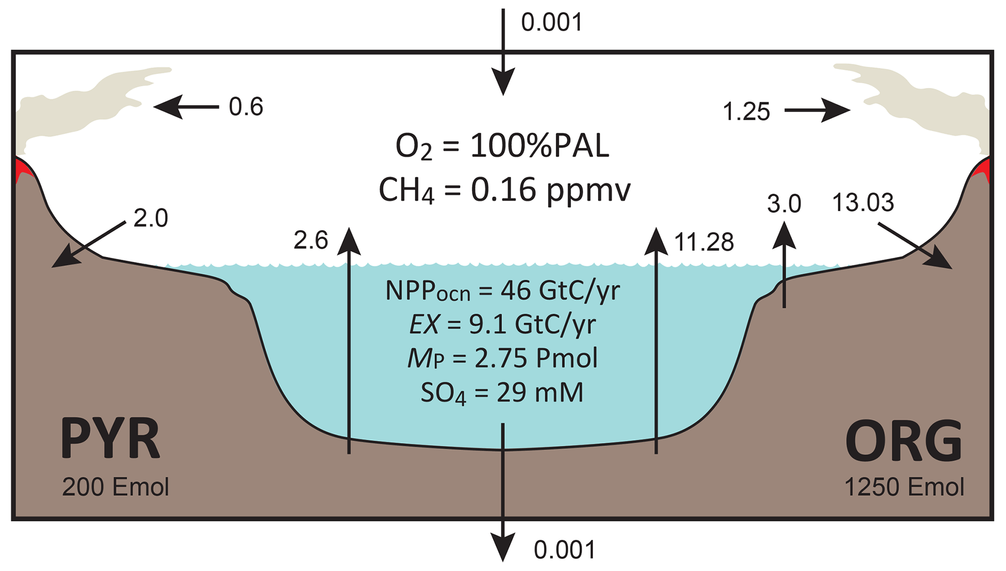
Figure 17 Schematics of global redox (O₂) budget for the reference run. Arrows represent the O₂ flux in terms of 10¹² mol O₂ equiv. yr⁻¹. PAL stands for present atmospheric level. Pmol is 10¹⁵ mol. Emol is 10¹⁸ mol. ORG represents sedimentary organic carbon. PYR represents sedimentary pyrite sulfur. NPP^ocn is oceanic net primary production. EX stands for export production. MP is oceanic phosphate inventory. SO₄ represents the concentration of sulfate.

4 Sensitivity experiment

Based on the results obtained above, we conclude that the CANOPS-GRB model is sufficient to describe basic biogeochemical characteristics in the modern ocean–atmosphere system. As a next step, we assess the dynamic response of the full model by performing sensitivity experiments with respect to P availability in surface environments.

4.1 Dynamic response to changes in P weathering

Here, we conduct a sensitivity experiment with respect to the P weathering rate in order to see how the atmospheric and oceanic O₂ levels respond to changes in P availability in the exogenic system over a wide range of timescales. Specifically, we performed four simulations, varying the values of f_P in Eq. (2) over 2 orders of magnitude. The reference state presented in the previous section is assumed for the initial condition, and the full model is allowed to evolve freely for 3 billion model years. These experiments demonstrate how P availability in surface environments affects global biogeochemical cycles and redox states of the atmosphere and oceans over a diverse range of timescales.

The simulated transient response is shown in Fig. 18. As expected, lower P availability leads to a lower oceanic P inventory (Fig. 18a), resulting in suppressed biological productivity in the ocean (Fig. 18b). Given the residence time of P in the ocean (18 kyr, see Sect. 3.2.3), these responses occur within 10⁵ years. The suppressed biological productivity leads a decline of burial rate of organic matter in sediments (Fig. 18c). Specifically, 10 % and 1 % of f_P give rise to the burial rate of marine C_org of 1 and 0.13 Tmol C yr⁻¹ at 10⁵ years, respectively (cf. the reference value of 11.3 Tmol C yr⁻¹).

On the timescales of 10⁵–10⁶ years, the system reaches a quasi-steady state, but there is still a large redox imbalance due mainly to the suppression of C_org burial (Fig. 18i). This gives rise to deoxygenation of the atmosphere on a timescale of millions of years (Fig. 18d). Note that once the ocean interior becomes anoxic, the enhanced P recycling and preservation of organic matter in anoxic marine sediments tend to buffer the atmospheric deoxygenation (Fig. 18a and c). However, these passive responses do not alter the fundamental behavior: lower P availability results in lower atmospheric O₂ levels. After atmospheric deoxygenation ($>\sim \mathrm{4}$ Myr), the system again reaches its quasi-steady state. Specifically, f_P values of 10 % and 1 % result in atmospheric O₂ levels of 9 % PAL and 0.6 % PAL, respectively.

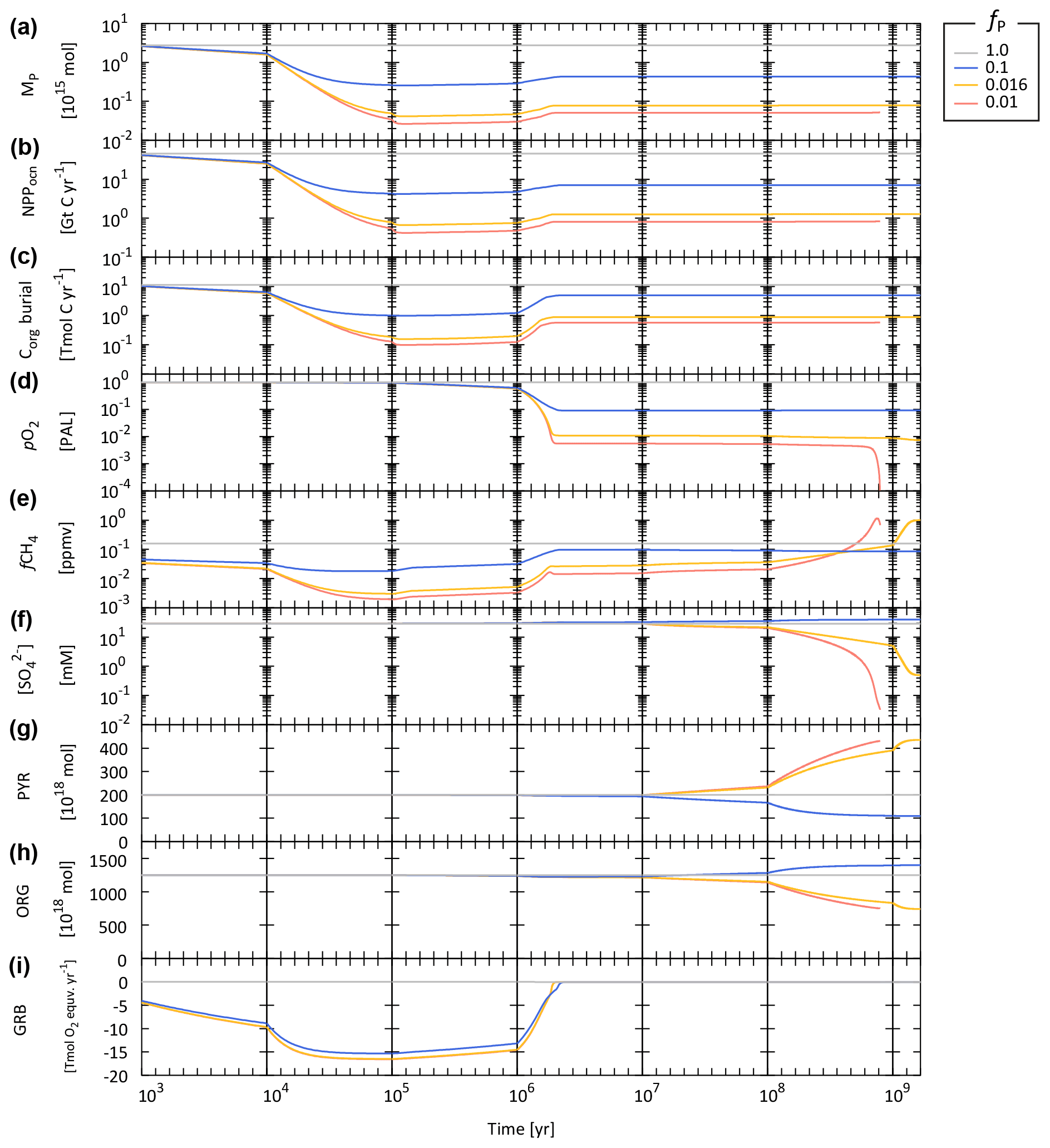
Figure 18 Biogeochemical responses obtained from the CANOPS-GRB model with different values of P availability, f_P. (a) Oceanic phosphate inventory, M_P. (b) Oceanic net primary production (NPP_ocn). (c) Burial rate of organic carbon (C_org) in marine sediments. (d) Atmospheric partial pressure of O₂. PAL stands for present atmospheric level. (e) Atmospheric CH₄ mixing ratio. (f) Sulfate concentration in the surface ocean layer. (g) Sedimentary reservoir size of pyrite sulfur (PYR). (h) Sedimentary reservoir size of organic carbon (ORG). (i) Global redox budget (GRB). For the f_P=1 % run (red line), the calculation stopped when the atmospheric O₂ level decreased to $\sim {\mathrm{10}}^{-\mathrm{5}}$ PAL due to the numerical instability.

The following change is driven by the response of oceanic S cycle, which is characterized by the long residence time of 11.5 Myr (see Sect. 3.2.5). Ocean anoxia promotes the MSR and subsequent precipitation of pyrite in the ocean interior. However, our model demonstrates that the decline of seawater SO${}_{\mathrm{4}}^{\mathrm{2}-}$ on a timescale of tens of millions of years is small (Fig. 18f) because the rate of MSR depends not only on the oceanic redox state but on the availability of organic matter for the MSR. The significant reduction of seawater SO${}_{\mathrm{4}}^{\mathrm{2}-}$ occurs on the longer timescales (>100 Myr) for extremely low f_P scenarios (0.016 and 0.01), in which atmospheric O₂ levels decrease to <1 % PAL. These scenarios also accompany a growth of sedimentary S from gypsum to pyrite (Fig. 18g).

On longer timescales, sedimentary reservoirs affect the redox state of the atmosphere and oceans. The present result demonstrates that f_P of 1 % finally leads to the catastrophic decrease in atmospheric O₂ level at around 0.9 billion years (Fig. 18d). The simulation was stopped at this point due to the numerical instability. For other scenarios, the system reaches a new steady state after roughly 3 billion model years.

Biogenic CH₄ production tends to be enhanced in anoxic oceans. However, the present result demonstrates that CH₄ degassing to the atmosphere is inhibited by both limited availability of organic matter for methanogenesis and the anaerobic oxidation of CH₄ by SO${}_{\mathrm{4}}^{\mathrm{2}-}$. Once seawater [SO${}_{\mathrm{4}}^{\mathrm{2}-}$] decreases below 1 mM, CH₄ can escape from oceans to the atmosphere, promoting the buildup of CH₄ in the atmosphere. Nevertheless, because of limited biological activity, atmospheric CH₄ levels remain comparable to the modern value (∼1 ppmv) (Fig. 18e).

4.2 O₂ budget for the less-oxygenated scenario

Figure 19 shows the O₂ budget of the less-oxygenated state (f_P=1.6 % scenario). Because P availability exerts a primary control on biospheric O₂ production, the strongly suppressed P delivery to the ocean leads to low oceanic P levels and commensurately low biological productivity (0.08 Pmol and 1.3 Gt C yr⁻¹, respectively). As a consequence, the atmospheric O₂ level is low (0.75 % PAL). In this scenario the ocean interior is globally anoxic, and the preservation of organic C in marine sediments is enhanced. However, the suppressed biological productivity results in a low overall burial rate of organic C (0.9 Tmol O₂ equiv. yr⁻¹; ∼9 % of the reference value). When combined with the burial rate of terrigenous organic C, total O₂ production by the organic C sub-cycle is 0.97 Tmol O₂ equiv. yr⁻¹. This O₂ source is balanced by the sum of oxidative weathering and metamorphism. The role of the pyrite S sub-cycle in the global redox budget is also shown in Fig. 19. Most of the SO${}_{\mathrm{4}}^{\mathrm{2}-}$ entering the anoxic ocean is buried as pyrite, representing a major O₂ source (2.64 Tmol O₂ equiv. yr⁻¹). This O₂ source is balanced by oxidation of sedimentary pyrite S through weathering (1.33 Tmol O₂ equiv. yr⁻¹) and metamorphism (1.31 Tmol O₂ equiv. yr⁻¹). In other words, the O₂ budget for the weakly oxygenated Earth system is largely affected by the crustal S sub-cycle. This is in marked contrast to the well-oxygenated Earth system, where the O₂ budget is mainly controlled by organic C sub-cycle.

The present result demonstrates that low atmospheric O₂ states (∼1 % PAL) can be achieved in scenarios where the availability of P is strongly limited. However, a slight decrease of f_P to 1 % leads to the destabilization of global O₂ budget, providing implications for the stability and evolution of atmospheric O₂ levels during the Proterozoic. This point will be further systematically examined in future work.

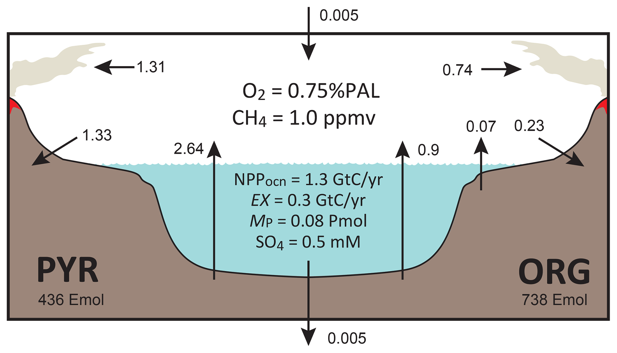
Figure 19 Schematics of global redox (O₂) budget for the f_P=1.6 % ($={\mathrm{10}}^{-\mathrm{1.8}}$) run. Arrows represent the O₂ flux in terms of 10¹² mol O₂ equiv. yr⁻¹. PAL stands for present atmospheric level. Pmol is 10¹⁵ mol. Emol is 10¹⁸ mol. Gt C is 10¹⁵ g C. ORG represents sedimentary organic C. PYR represents sedimentary pyrite S. NPP^ocn is oceanic net primary production. EX stands for export production. MP is oceanic phosphate inventory. SO₄ represents the concentration of sulfate.

5 Discussion

The reference run under the present condition demonstrates generally good agreement with modern observations (Sect. 3). The water circulation scheme provides an adequate representation of general ocean circulation, resulting in robust and reliable tracer distributions that are comparable to the modern observations. This provides a mechanistic foundation for simulating generalized ocean biogeochemical cycles. The ocean biogeochemistry module includes a series of biogeochemical processes in oxic–anoxic–sulfidic environments. The reference run gives rise to the distributions of nutrients and dissolved O₂ that capture fundamental properties observed in the modern ocean. Integrated biogeochemical fluxes of the global ocean, such as biological productivity, material flow in the water column, and burial into sediments are also consistent with observational data. In our reference run the estimated organic carbon burial and oxidative weathering fluxes are relatively high compared to some previous estimates, though there remains significant uncertainty in globally integrated organic carbon weathering and burial fluxes. Further work will also be needed to better quantify the biogeochemical cycling in the continental shelf, which is a major locus of organic matter burial. In addition, some future developments to the N cycle may be needed, especially with regard to denitrification (e.g., anammox, coastal benthic denitrification). Despite these remaining challenges, our biogeochemical model is adequate for representing the general property of the coupled C–N–P–O₂–S cycles.

A new scheme for oxidative weathering of organic matter and pyrite sulfur, mass balance calculation of O₂ in the atmosphere, and time evolution of sedimentary reservoirs are explicitly included in the CANOPS-GRB model. These are a significant improvement from the previous versions of CANOPS (Lenton, 2020). The simplified framework for the global O₂ budget is also useful to understand the response of complex biogeochemical systems. The computational efficiency of our CANOPS-GRB model allows us to conduct simulations over billions of model years with reasonable wall times (on the order of weeks), providing a useful tool for exploring the wide range of topics about the oxygenation history of Earth's atmosphere.

Sensitivity experiments with respect to the terrestrial weathering rate of P were conducted in order to see how the redox state of the ocean–atmosphere system responds to varying P availability in the surface system (Sect. 4). The CANOPS-GRB model appears to adequately simulate the biogeochemical dynamics over a wide range of timescales and is applicable for quantitative assessment of the evolution and stability of Earth's O₂ cycling. Perhaps even more importantly, our results encourage us to perform further systematic examinations with Earth system models that have different complexities. Such an “Earth system model intercomparison” would be a critical step towards better mechanistic understanding of the stability and dynamics of atmospheric O₂ levels over Earth's history.

Due to a lack of explicit Fe cycling and anaerobic metabolisms (such as anoxygenic photosynthesis), the current version of the model cannot be applicable for the simulation under the Archean-like weakly oxygenated (pO${}_{\mathrm{2}}<{\mathrm{10}}^{-\mathrm{5}}$ PAL) conditions. These topics are left to future studies, but it would be an achievable goal (Ozaki et al., 2018, 2019b; Van De Velde et al., 2021). The model design presented here also ignores the interaction between the surface system and the mantle (e.g., subduction) except for the degassing of reducing gases from the mantle. We note, however, that the surface–mantle interaction would have exerted a primary control on the long-term redox budget of Earth's surface system through the Earth's history (Canfield, 2004; Eguchi et al., 2020; Hayes and Waldbauer, 2006) and may be important for the discussion about the distant future (Ozaki and Reinhard, 2021). The importance of mantle and solid Earth controls on surficial environments is a crucially important topic for future research.

The CANOPS-GRB model has the basic capability to simulate the time evolution of the abundance of atmospheric biosignature gases (O₂ and CH₄) on a wide range of timescales. While the biogeochemical model is based on process studies to the extent possible, many processes are derived from empirical calibrations to Earth-like planets around Sun-like stars. Clearly, some these parameterizations, such as the photochemical parameterization among O₂–O₃–CH₄ (Eq. 107), must be modified when applying the model to a range of habitable Earth-like exoplanets.

6 Conclusions

A new Earth system box model was developed – CANOPS-GRB v1.0. The new code release provides an improved description of the coupled C–N–P–O₂–S biogeochemical cycles in the ocean–atmosphere–crust system, which can be utilized to examine the dynamics and stability of Earth's O₂ cycle over a wide range of timescales. The computational efficiency and simple model design of CANOPS-GRB make it relatively easy to modify existing processes or add entirely new processes and components. CANOPS-GRB is thus a new and uniquely flexible tool capable of providing a coherent mechanistic framework for quantifying the biogeochemical cycles regulating Earth's O₂ cycle. CANOPS-GRB is also a useful tool for the development of more comprehensive, low- to intermediate-complexity Earth system box models of biogeochemistry.

CANOPS-GRB provides an important step forward when coupled to new and existing geochemical proxy data. The accumulating geological and geochemical records have led to a new hypothesis for the evolution of atmospheric O₂ levels on Earth. CANOPS-GRB was designed to facilitate simulation of a wide range of past conditions so as to permit more explicit testing of hypothesis about the function of biogeochemical cycles and their effect on the redox budget throughout Earth's history. Through the model–data synergy, CANOPS-GRB has great potential to provide an integrated, quantitative, and statistically informative picture of biogeochemical states, opening new perspectives on a wide range of scientific questions in research seeking to understand Earth's chemical evolution and the cause-and-effect relationships with evolving biosphere in particular.

CANOPS-GRB also provides significant steps forward in our predictive understanding of the links between geology, biogeochemistry, and the evolution of Earth's biosphere. It will allow for a fundamentally new and more precise quantitative understanding of evolving atmospheric biosignatures (O₂, O₃, CH₄) on Earth and will broaden the interpretive power of Earth system evolution in the search for life beyond our planet. Additional elaboration of the CANOPS-GRB code could represent an important avenue for developing a more robust tool for diagnosing atmospheric biosignatures for future analysis of extrasolar worlds. In summary, it is anticipated that CANOPS-GRB will have many applications for problems linking the coupled evolution of life and the atmosphere on Earth and habitable rocky exoplanets.