the Creative Commons Attribution 4.0 License.
the Creative Commons Attribution 4.0 License.
 | 18 Oct 2022
TrackMatcher – a tool for finding intercepts in tracks of geographical positions
Peter Bräuer
Matthias Tesche
Working with measurement data in atmospheric science often necessitates the co-location of observations from instruments or platforms at different locations with different geographical and/or temporal data coverage. The varying complexity and abundance of the different data sets demand a consolidation of the observations. This paper presents a tool for (i) finding temporally and spatially resolved intersections between two- or three-dimensional geographical tracks (trajectories) and (ii) extracting observations and other derived parameters in the vicinity of intersections to achieve the optimal combination of various data sets and measurement techniques.
The TrackMatcher tool has been designed specifically for matching height-resolved remote sensing observations along the ground track of a satellite with position data of aircraft (flight tracks) and clouds (cloud tracks) and is intended to be an extension for ships (ship tracks) and air parcels (forward and backward trajectories). The open-source algorithm is written in the Julia programming language. The core of the matching algorithm consist of interpolating tracks of different objects with a piecewise cubic Hermite interpolating polynomial with the subsequent identification of an intercept point by minimising the norm between the different track point coordinate pairs. The functionality wrapped around the two steps allows for the application of the TrackMatcher tool to a wide range of scenarios. Here, we present three examples of matching satellite tracks with the position of individual aircraft and clouds that demonstrate the usefulness of TrackMatcher for application in atmospheric science.
- Article
(2945 KB) - Full-text XML
-
Supplement
(10353 KB) - BibTeX
- EndNote


In atmospheric science, data from different measurement platforms or locations are often combined for synergistic analysis or validation purposes. This holds true particularly for the combination of measurements from different spaceborne sensors, e.g. Sun-Mack et al. (2007), Kato et al. (2011), Redemann et al. (2012), or Alfaro-Contreras et al. (2017), and the long-term validation of those measurements at ground sites, e.g. Pappalardo et al. (2010) and Tesche et al. (2013). The co-location problem is particularly relevant for mobile observations (airborne, ship-based, or spaceborne observations) with active sensors such as lidar or radar. In contrast to passive sensors with a swath width of the order of 1000 km, active sensors provide height-resolved measurements along a very narrow ground track, with so-called curtain observations below or above the track of the platform that carries the respective instrument.
In the past, observations with the Cloud-Aerosol Lidar with Orthogonal Polarisation (CALIOP) aboard the Cloud-Aerosol Lidar and Infrared Pathfinder Satellite Observations (CALIPSO; Winker et al., 2009) satellite or the Cloud-Profiling Radar (CPR) aboard the CloudSat satellite (Stephens et al., 2002) have been matched with (i) backward (forward) trajectories arriving (starting) at a specific ground site (Tesche et al., 2013, 2014), (ii) ship tracks in decks of stratiform clouds (Christensen and Stephens, 2011), (iii) linear contrails, as identified from passive remote sensing (Iwabuchi et al., 2012), or (iv) flight tracks of aircraft (Tesche et al., 2016). The TrackMatcher tool has been developed to enable a unified and objective way of finding temporal and spatial matches between the ground tracks of satellites or research aircraft that perform height-resolved observations of atmospheric parameters and spatiotemporal information (tracks) of ships, aircraft, clouds, or air parcels. In addition to the information on time and location that is needed to perform the matching, the algorithm handles auxiliary data along the considered tracks and enables co-locating and sub-sampling of the along-track data sets. The technical details and the performance of the TrackMatcher algorithm are described in Sect. 2. Examples of the application of the tool are provided in Sect. 3. We conclude this work with a summary and an outlook of the potential fields of application of the developed algorithm in Sect. 4.
2.1 Motivation
The purpose of TrackMatcher is the identification of intercept points between two time-resolved three-dimensional paths of latitude/longitude/height () coordinates (referred to as tracks or trajectories hereafter) and the collection of the respective data fields along those tracks. Tracks may be reduced to two dimensions, e.g. for objects moving at ground level or, in the case of satellite data, saved as curtains, where the column profile above the ground track position is stored.
TrackMatcher operates on a primary data set with individual (usually short) trajectories. The tool is designed for flight track and cloud track data, but any individual three-dimensional trajectory can potentially be incorporated into TrackMatcher. These primary trajectories are matched to a single, potentially very long, trajectory in a secondary data set that could span the Earth several times. In the current version of TrackMatcher, cloud layer and profile data from the CALIOP instrument aboard the CALIPSO satellite are used, and it is planned to expand to aerosol layer and profile data as well. For performance reasons, the secondary trajectory is stored as segments, which enables the TrackMatcher package to be easily expanded to compare to two sets of individual trajectories. A detailed overview of the data structure in TrackMatcher is given in Sect. 2.3. The package features options regarding (i) the format of the input data from text files with comma- (csv) or tab-separated values (tsv) or from HDF4 or MATLAB mat files, (ii) the configuration of the output fields, and (iii) the optimisation of the balance between performance of the algorithm and accuracy of the results. A detailed description of the settings can be found in Sect. 2.5.
While we refer to the general terms of primary and secondary data in this paper, the motivation for developing TrackMatcher was the desire to find intersections between the three-dimensional flight tracks of individual aircraft (primary data) and curtain observations along satellite ground tracks (secondary data). Specifically, the position of aircraft and auxiliary information, such as the type of aircraft, engine, and fuel, should be matched to vertically resolved extinction coefficients from a spaceborne lidar measurements to assess the environmental and climate impact of an aircraft passage through a cirrus cloud (Tesche et al., 2016).
For this purpose, TrackMatcher ought to process two types of spaceborne observations along the satellite ground track related to information on (i) column parameters for cloud or aerosol layers and (ii) vertically resolved observations (profiles) within those cloud or aerosol layers. The algorithm was designed to operate with aircraft location data available from online flight trackers (e.g. https://flightaware.com/, last access: 12 October 2022) or databases that provide position data for individual aircraft (Brasseur et al., 2016). The large volume of the considered position data for matching with an abundance of satellite track data, together with the overall low match rate of the two, requires an automated and objective procedure that is realised in the TrackMatcher tool.
Despite the initially highly specific scope for developing TrackMatcher, the tool is useful for a much wider range of applications that require matching time, position, and auxiliary data along two tracks on a geographic grid. Potential applications include matching vertically resolved information along satellite tracks with (i) tracks of individual clouds (see Sect. 3.3 and Seelig et al., 2021), (ii) ship tracks or (iii) trajectories of air parcels from dispersion modelling, or even (iv) matching three-dimensional flight data with three-dimensional cloud tracks. While the current focus of TrackMatcher is on applications in atmospheric science, the tool is designed for great flexibility with respect to the input data for further applications in the wider geosciences.
2.2 Code availability and package dependencies
TrackMatcher is an open-source package hosted at GitHub (https://github.com/LIM-AeroCloud/TrackMatcher.jl.git, last access: 12 October 2022) under the GNU General Public License v3.0. We strongly encourage contributions from outsiders, e.g. by pull requests or filing issues.
TrackMatcher is written in Julia (Bezanson et al., 2017). The package relies on a licensed MATLAB version to read the satellite data from HDF4 files. The software is distributed as an unregistered Julia package and is tested against the Julia long-term support version 1.6.x and the most recent stable release (1.x).
The PCHIP package was developed within the TrackMatcher framework to allow a track interpolation with a piecewise cubic Hermite interpolating polynomial (see Sect. 2.4). It is available under the GNU General Public License v3.0 at GitHub (https://github.com/LIM-AeroCloud/PCHIP.jl.git, last access: 12 October 2022).

2.3 Data structure
TrackMatcher is organised in data sets making use of Julia's type system. For readers unfamiliar with the type system, Sect. S1.1 in the Supplement highlights the key points of this ecosystem and the different types.
Figure 1 shows TrackMatcher's type tree. Abstract types (blue boxes) are used internally to classify concrete types (green boxes) that actually store data. Data are loaded into TrackMatcher, or computation is started by instantiating a type or struct, i.e. a function with the name of the data type is called a so-called constructor that triggers a TrackMatcher process and saves data in a type of the same name. Those constructors that can initiate a TrackMatcher process are circled in purple in Fig. 1. Light blue boxes in Fig. 1 are special cases. In these boxes, the top white label denotes an abstract type that is used for data classification, while the bottom grey label points to the concrete type that stores the data. However, it is the user's choice to call a function with either the top or bottom name to save data in the concrete type. Below, the TrackMatcher types are explained in more detail. Types that can initiate a TrackMatcher are highlighted together with the data that are stored in each type.
In TrackMatcher, the top level type is a generic DataSet, which holds data with fields for measured (MeasuredSet) and computed (ComputedSet) data. The MeasuredSet organises the track data and observations. Observations are subtypes of the ObservationSet, as shown in Fig. 1. Track data are split into primary and secondary data sets. Currently, primary data consist of individual trajectories (a PrimaryTrack) that are combined into a PrimarySet. The current version of TrackMatcher distinguishes between flight and cloud data in the PrimarySet and PrimaryTrack. Within the FlightSet, a FlightTrack can be obtained from several sources; however, the format of FlightData is unified. Currently, the only SecondarySet is SatSet. The main difference between track data in the PrimarySet and SecondarySet is that primary data consist of a potentially large number of smaller individual tracks, while secondary data are stored in a single long trajectory. However, for performance reasons, secondary data are split into track segments. Segments are stored in the field granules of SatSet. Segments or granules are classified below the SecondarySet level as SecondaryTrack, which currently only hold the SatData of the SatTrack. Each SatTrack is a track segment of the satellite track from either the day- or nighttime hemisphere of Earth loaded from the individual input files. Intersection data (or XData) with intercept points from the primary and secondary trajectories are stored as a child of the ComputedSet, with no distinction which primary data type was used for the calculation.
2.4 Algorithm description
The key steps of the algorithm are to (i) load track data related to two platforms, (ii) interpolate the individual tracks, (iii) find intersections by minimising the norm between the different track point coordinate pairs, and (iv) extract auxiliary information at or around the intercept point as set by the operator. These steps are described in the subsequent subsections, with examples for matching aircraft or cloud position data with satellite ground tracks given in Sect. 3, as motivated by Sect. 2.1.
Intersections between two tracks are defined as those locations for which the distance between a pair of points from the primary and secondary track reaches zero. This distance can be calculated either as the difference in the latitude values from two tracks with a common longitude value or as the difference in the longitude values for a common latitude value. The general form of the distance function is as follows:
Here, x is either a latitude or longitude value, and represent the primary and secondary trajectories that determine the corresponding longitude and latitude values. The roots of Eq. (1) define the intercept points between both tracks.
2.4.1 Track data import
Primary and secondary data are loaded from provided files (currently csv, tsv, mat, or hdf) and stored in a unified format in the respective structs of the type tree presented in Fig. 1. Time-resolved track points of the individual trajectories and other relevant data at these points are stored in a field data that consist of a DataFrame, with columns for each property and rows for every time step. Additional database information and overall information concerning the trajectory as a whole are stored in the metadata field of the primary data.
For the primary data, individual tracks from one source are loaded to a vector, which in turn are combined in the PrimarySet of the respective data type (FlightSet or CloudSet). Each PrimarySet can have several fields for the vectors of PrimaryTrack. The structures of the primary data currently available in TrackMatcher, according to the examples presented in Sect. 3, are visualised in Fig. S3 in the Supplement.
Secondary track data are stored as segments of a continuous track for performance reasons (see also Sect. 2.3). All track segments are combined in a set. Secondary track data (currently only SatData) are stored in a data field, with a DataFrame using the same structure as primary data (see Fig. S2 for schematics of the current data structure). Only essential data needed for the calculation of intersections are stored in this struct for performance reasons, i.e. time, latitude, and longitude. All SatData are combined in the field granules of the SatSet. Additional information about the temporal and spatial coverage of each granule and the location of the input file is given in the SatSet metadata.
Observations at track points are only extracted from the input files if intercept points between the primary and secondary track sets are found. Specifics regarding the extracted data can be customised for the desired application.
2.4.2 Track data interpolation
A fundamental problem of the TrackMatcher algorithm is that the true functions of the investigated tracks are unknown and have to be approximated. The approximation is only valid near nodes, i.e. in the vicinity of known track points. For Eq. (1) to be applicable, x (either latitude or longitude) must be equal for both tracks. In reality, the two tracks rarely feature regular intervals and most likely will not share a common latitude or longitude vector. Hence, both data sets will first need to be interpolated with a common set of x data between a shared start and end value.
Generally, track data cannot be fitted to a known function, and the connection between latitude/longitude pairs needs to be approximated with a suitable interpolation method. We chose the Piecewise Cubic Hermite Interpolating Polynomial (PCHIP; see, e.g. Fritsch and Carlson, 1980; Kahaner et al., 1989; Turley, 2018) to approximate a function f(x) between any two data points, xi and xi+1, as follows:
Polynomials in Eq. (2) are defined as follows:
and
The PCHIP method demands a continuous first derivative f′(x) at each data point (node) but, in contrast to cubic splines, does not require a continuous second derivative f′′(x). This principally means that cubic splines are slightly more accurate in approximating continuous curves. For our purpose, the decreased accuracy is negligible and well within the errors in the track data points themselves. Instead, PCHIP interpolation suppresses artificial oscillation at discontinuities which can occur at sharp turns of a track.
Track interpolation is a comprehensive task that consumes a significant portion of the source code. Therefore, PCHIP has been outsourced as a separate package, which is available at GitHub under the GNU General Public License v3.0 or above (https://github.com/LIM-AeroCloud/PCHIP.jl.git, last access: 12 October 2022).
2.4.3 Calculation of intercept points
To find intercept points between the primary and secondary tracks, the TrackMatcher algorithm follows seven steps that are explained in more detail below:
-
Load primary data nd find the prevailing track direction and inflection points in the x data of the primary track.
-
Load secondary data for the time frame of the primary data, including a pre-defined tolerance at the beginning and end, and find inflection points in the x data based on the prevailing track direction of the primary data.
-
Put a bounding box around the coordinates of the primary track (see Fig. 2) and find segments of the secondary track within these coordinates and a given window of acceptable temporal difference ±Δt.
-
Interpolate the track segments of the primary and secondary tracks with the PCHIP method using common equidistant x data with a defined step width.
-
Define a function (Eq. 1) to obtain the roots between the difference in the track points of both tracks.
-
Take the roots of Eq. (1) as the intersections between both tracks.
-
Filter intersections and save intersection data and relevant measurements from the input data in the vicinity of the intercepts.
The result of the procedure is visualised in an example of an aircraft flight track and a satellite ground track in Fig. 2.
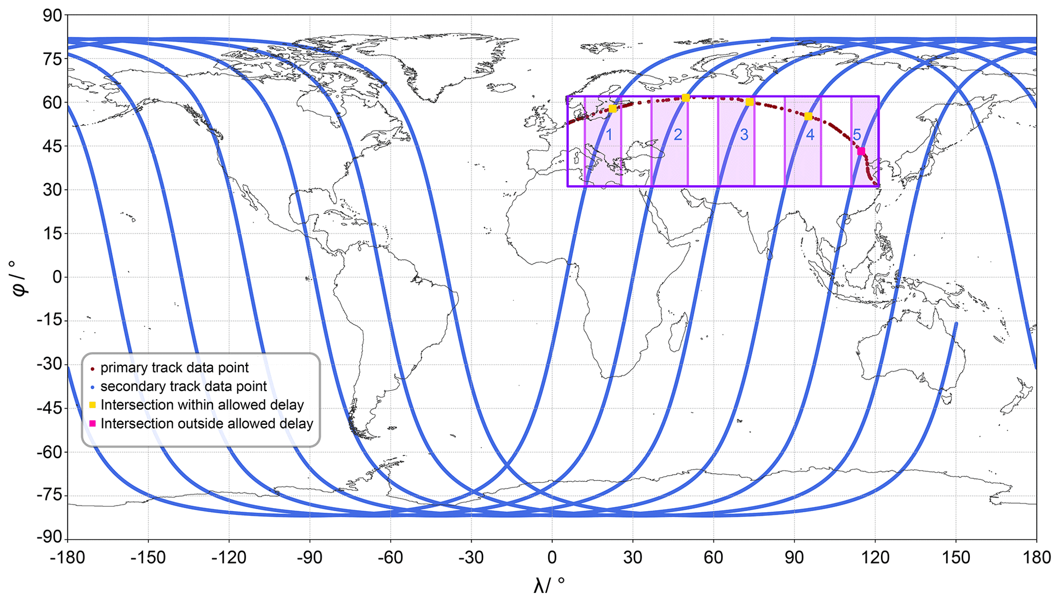
Figure 2Example plot of flight (primary) and satellite (secondary) track data and the intersections found by the algorithm.
Track data are loaded (steps 1 and 2) as explained in Sects. 2.4.1 and 2.5.2. For the interpolation of the track data of both trajectories in step 4, strictly monotonic ascending x data are a requirement. Therefore, both trajectories are fragmented into segments that fulfil this condition. To minimise fragmentation, the prevailing direction (north–south or east–west) of the primary track is determined while reading the input data according to the following:
with
Longitude λ is chosen as the x value if Eq. (10) is true and the dominant direction of the primary track is east–west. Otherwise, latitude φ performs better for a prevailing north–south direction. In Eq. (10), maximum horizontal distances are calculated separately for positive (λ+) and negative (λ−) longitude values to avoid problems with the sign change at the date line. The last term on the right-hand side of Eq. (10) corrects for the poleward decreasing distance between meridians. For simplicity, only the mean latitude () is considered. As highly irregular patterns are currently only expected in the primary track, their data define whether φ or λ are used as x data in both tracks.
Before interpolation, data of the secondary track need to be extracted for the correct time frame and location in step 3. Therefore, only data points are considered that are within the time span of the primary data. Additional data points at the beginning and end are allowed to permit a delay at the possible intercept points of the primary and secondary track. By default, a maximum delay of 30 min is permitted, which can be adjusted by the user. To exclude unnecessary secondary track data, only those track points within the range between the minimum and maximum latitude/longitude values are considered. To avoid problems at the date line, minimum/maximum values for longitude values are considered separately for negative and positive longitude values. This creates a bounding box around all track points, as depicted in Fig. 2 (violet box). Only track segments of the secondary trajectory within this bounding box are considered in any further steps (visualised by the pink shaded areas 1 to 5 in Fig. 2). To allow for rounding errors, the bounding box can be increased by an absolute tolerance (by default 0.1∘), which is added to the maximum value and subtracted from the minimum value.
In step 4, all segments are interpolated. Common x data are used in the overlapping regions (pink boxes in Fig. 2). These segments ( in Eq. 1) are used for the identification of intercept points. Equation (1) is case specific and is redefined for every segment pair (or box) in step 5. In step 6, TrackMatcher uses the IntervalRootFinding.jl package to determine all the roots of Eq. (1). These roots are intercept points between the tracks of the primary and secondary data set.
In rare cases, the algorithm duplicates intercept points. This occurs mainly when an intercept point is located at a track segment boundary where matches are then found on either side of the segment border. Duplicate intercepts can also occur in case of near-parallel tracks. To avoid the output of duplicate detection, the algorithm verifies that only the intercept calculation with the highest interpolation accuracy is stored within a predefined radius. By default, this radius is 20 km but can be customised by the user.
Duplicate intercept points and intercept points for which the delay between the primary and secondary track exceeds a specified time difference are disregarded in step 7 (pink square in Fig. 2). This and further filtering is controlled by keyword arguments at the start of a TrackMatcher run, as outlined in Table 1. For the remaining intercept points (yellow squares in Fig. 2), the latitude, longitude, respective times of the primary and secondary track at the intercept point, and the difference between these times, details regarding the interpolation accuracy, and user-selected auxiliary data in the vicinity of the intercept points are saved.
Linear interpolation between recorded time steps of the track points is used to derive the exact intercept time. Accurate interpolation, as with the PCHIP method, demands track segments with strictly monotonic latitude and longitude data (see Sect. 2.4.2). This likely results in a strong segmentation of the original track and leads to high computational costs. However, satellites, clouds, and aircraft at cruising altitudes are expected to move with relatively constant velocity, which is why linear interpolation can be applied to derive the time of intercept. For ascending and descending aircraft with unknown acceleration or deceleration, track points are close to each other, leading to minimal errors from linear interpolation.
To calculate the distance between track points, which is needed for setting a variety of thresholds, we use the haversine function as follows:
which gives the great circle distance between two points on a perfect sphere. In Eq. (12), are the latitude values of the coordinate pairs 1 and 2, are the respective longitude values, and r is the radius of a perfect sphere. The poleward decrease in the Earth's radius is approximated as follows:
with req=6 378 137 m and rpol=6 356 752 m as the radii on the equatorial and polar planes, respectively.
Table 1Parameters controlling TrackMatcher runs. Arguments are printed italic, keyword arguments use roman font.

2.5 Programme description
2.5.1 General information and package installation
This paper describes TrackMatcher version 0.5.3 and PCHIP version 0.2.1. A wiki with a complete manual is available from the TrackMatcher repository at GitHub. Here, only the most important aspects of the tool and its usage are highlighted. The programme description is not meant to be a complete set of instructions. Further guides and examples can be found in Sect. S2 in the Supplement.
With version numbers below 1.0, breaking changes may still occur frequently at the introduction of new minor versions. However, this eases the introduction of new features or the improvement in current routines. Contributions from outsiders, e.g. by pull requests or filing issues, are strongly encouraged to enhance the performance and flexibility of the algorithm.
Both TrackMatcher and PCHIP are unregistered Julia packages. The easiest way to install them is by using Julia's built-in package manager and adding the uniform resource locator (URL) of the GitHub repository. Example code for TrackMatcher installation is shown in Script 1 in Sect. S2.1 in the Supplement. This will install the package and all dependent registered Julia packages in the correct version, as defined by the package's project file. However, dependent unregistered packages need to be installed manually prior to the actual package installation. Therefore, the order of installation for TrackMatcher must be as follows:
-
PCHIP.
-
TrackMatcher.
Package developers can use the dev option in Julia's package manager. However, it is recommended to clone the TrackMatcher repository from GitHub and activate the main folder with the Project.toml file to develop and run TrackMatcher.
Moreover, TrackMatcher relies on a Julia installation of at least version 1.6, with long-term support given for version 1.6 and further support for the current stable minor release. Additionally, TrackMatcher requires a licensed MATLAB version. If your MATLAB version is not installed in the standard directory of your system, it needs to be linked to Julia, as described by Julia's MATLAB package README (https://github.com/JuliaInterop/MATLAB.jl.git, last access: 12 October 2022). Further help for linking MATLAB to Julia can be acquired from the package's resources.
2.5.2 Loading input data
Currently, TrackMatcher is configured to process the following three types of data:
-
aircraft track data from different sources (stored as primary data in FlightData/FlightSet),
-
cloud track data (stored as primary data in CloudData/CloudSet), and
-
CALIPSO satellite data (stored as secondary data in SatData/SatSet).
Track data are stored in structs with a data field and, for primary data, a metadata field. Metadata are another struct with information about the raw data, computation settings and times, and properties concerning the whole trajectory. Time-resolved data are stored in a DataFrame in the data field with the columns time, lat, and lon and further columns, depending on the data type (aircraft, cloud, or satellite data).
Tracks from primary data sets are stored in individual structs, which are combined in a vector and stored in a database struct (FlightSet or CloudSet) together with metadata (see Sect. 2.3 and the Supplement for details). Several databases, e.g. individual flight tracks saved in tsv files or complex flight inventories, are considered for aircraft data. Each database type is stored in a separate vector/FlightSet field.
In contrast, secondary data consist of a single long trajectory. However, for performance reasons, data are stored as SatData structs for individual granules (track segments holding data of either the day- or nighttime hemisphere of Earth). Moreover, only time, latitude, and longitude are stored in SatData for an optimised performance.
Further satellite data are only loaded in the vicinity of intersections. Currently, additional satellite data can be extracted either as a height profile (CPro) or as a layer mean value (CLay). The additional data are also used to determine the meteorological conditions at the intersection. Only one type of the observation data (CPro or CLay) can be used to derive intercept points. The data type is determined automatically from the keyword CPro or CLay embedded in the file names. If both type exists, the data type with a majority in the first 50 files is chosen, unless the default behaviour is overwritten by user settings. It should be noted that profile data give a more refined height resolution and, hence, a more precise representation of the height-resolved atmospheric state at the intersection at the cost of more memory usage and a longer computation time.
Data are loaded from HDF4, MATLAB data (.mat) files, or text files with comma-separated values (csv) or tab-separated values using tsv, dat, or txt as file extension. Details on the database types, file formats, restrictions and conventions can be found in Sect. S2.2.1 in the Supplement.
To load data into the respective struct, a convenience constructor exists that takes any number of file strings with absolute or relative folder paths as input. These directories and all subfolders are searched recursively for any file with the correct extension. These files are assumed to be valid data files or will produce a non-critical error during loading. Further keyword arguments control data reading and filtering, as given in Table 1.
Aircraft data are currently the only data type with multiple database sources. For the data files, csv is a commonly used file format. Therefore, data files cannot be identified by file extension alone, as this does not allow an assignment to the correct database. Therefore, directories are passed as strings to keyword arguments for the respective database type. If a user wants to scan more than one directory for the same database type, a vector of strings can be passed to the keyword arguments (see Sect. S2.2 and Note 7 in the Supplement for details).
2.5.3 Calculating intersections and model output
To calculate intersections between the trajectories of the primary and secondary data sets, the user only needs to instantiate a new Intersection struct using either FlightSet or CloudSet and SatSet as input to a modified constructor for Intersection. The algorithm works only for either flight or cloud data, and two intersection structs need to be instantiated if you want to calculate intersections for both types. However, the algorithm does not differentiate between the different flight database types and calculates intersections for all flights in a FlightSet regardless of the source. Parameters exist to control the performance and accuracy of the results, as indicated by Table 1 and detailed in Sect. S2.2.3 in the Supplement.
Results are stored in the fields of Intersection. Each field of intersection, observations, and accuracy contains a DataFrame with the spatial and temporal coordinates of the intersection, measured data in the vicinity of the intersection, and indicators for the interpolation accuracy, respectively. The DataFrame columns consist of different parameters in each category, and DataFrame rows hold data for different intersections. The different fields are linked through an ID number, which makes identification of data belonging to the same intersection easier than solely having to rely on identification by DataFrame row. Table 2 explains the output format. An additional field with metadata exists in struct Intersection detailing the conditions of the TrackMatcher run (see also Fig. S4 in the Supplement).
Table 2Column names in the DataFrames of the Intersection fields together with the corresponding data types and units.
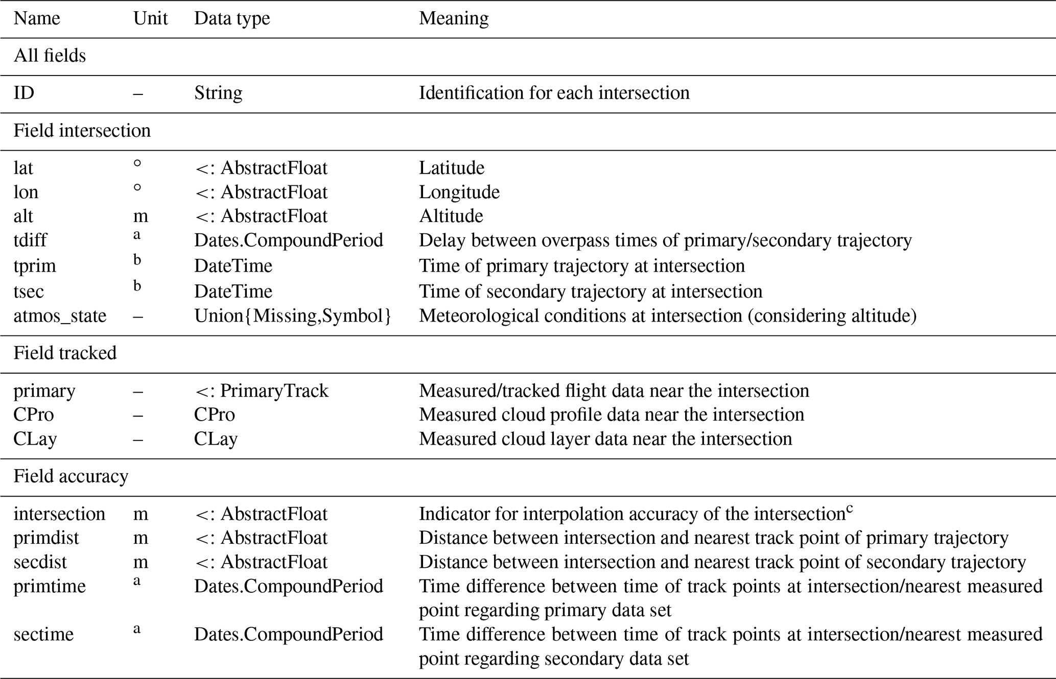
a Units are given in the CompoundPeriod and range from milliseconds to years. b DateTime in the format yyyy-mm-ddTHH:MM:SS. c Interpolation accuracy level is derived by using the interpolated trajectory of the primary and secondary data set to calculate the complete coordinates of the intersection. The difference in metres between both calculations is the interpolation accuracy parameter.
2.5.4 Adapting TrackMatcher
The TrackMatcher package works as is for the track data described in this article, with the prior installation of a licensed MATLAB version and an installation of the PCHIP.jl package (https://github.com/LIM-AeroCloud/PCHIP.jl.git, last access: 12 October 2022). If MATLAB is installed in the default system folder, then the link to Julia should work without any further set up. Otherwise, users need to turn to the installation guide of the Julia MATLAB package (https://github.com/JuliaInterop/MATLAB.jl.git, last access: 12 October 2022).
For correct data processing, there are data formats and file naming conventions that need to be adhered to. Particularly, folder and file names of satellite data need to include keywords CPro or CLay and, if both data types are saved, need to be identical, except for those keywords (see also Note 4 in the Supplement). Aircraft track data from web content need to include the flight ID, start date of the flight, and the International Civil Aviation Organization (ICAO) codes for the origin and destination (see Note 2 in the Supplement).
Users outside central Europe will have to add time zone support in the main file TrackMatcher.jl, as explained in Sect. 2.2.1 in the Supplement with details given in Note 5 and code example 1. This allows users to operate with a ZonedDataTime for web data saved as local time.
In general, structs within the type tree presented in Fig. 1 exist to load and store input data from the primary and secondary trajectories or observations near intersections. Further structs calculate and store intersection data and meta information.
When adapting code, developers should obey this general structure. If the file format of a database has changed, then the respective routines should be updated. To add new track data, new track structs should be added to an existing or newly established PrimarySet or SecondarySet. Section S3 in the Supplement helps developers to understand the general structure of the source files and the contained functions.
Data should be added in a way such that all track data of the same data set are stored in a unified format. For example, all track data of the FlightSet are stored as a FlightData struct, regardless of the source of the flight data. If users want to add data from another source, then these data should be stored in FlightData structs as well, saving identical information. If the need arises to save additional data, structs responsible for storing the data should be altered. If the data are not available in previous databases, filler objects such as missing, nothing, or NaN should be used.
This section presents three example applications of the TrackMatcher algorithm related to the authors' research focus of finding intercepts between the ground track of the CALIPSO satellite and (i) tracks of individual aircraft from the regional data set used by Tesche et al. (2016), (ii) 1 month of aircraft tracks from a global flight inventory for the year 2012, and (iii) tracks of individual clouds as identified from geostationary observations (Seelig et al., 2021). The first two applications are focussed on studying the effect of aviation on climate (Lee et al., 2021), while the third application marks a novel approach for investigating aerosol–cloud interactions (Quaas et al., 2020) and particularly the effect of aerosols on the development and lifetime of clouds.
3.1 Revisiting intercepts determined by Tesche et al. (2016)
Tesche et al. (2016) studied the effect of contrails that formed in already existing cirrus clouds. For their work, they investigated 37 799 flight tracks for three round-trip connections from airports in California, USA (Los Angeles, San Francisco, and Seattle), to Honolulu, Hawaii, USA, in the years 2010 and 2011. Intercept points were calculated for these tracks with the CALIPSO satellite ground track. While Tesche et al. (2016) used a method for finding intercepts between the two tracks that was fit for purpose, this method was less sophisticated and less generalised than is now realised in TrackMatcher. Specifically, few intercepts were found over the ocean, where aircraft positions are not measured with Automatic Dependent Surveillance–Broadcast (ADS-B) receivers but generally interpolated geodetically with a distance of about 1 h between consecutive points. This is likely related to the uneven interpolation (number of points rather than fixed distance) between the points of these segments.

Figure 3Occurrence rate of (a) intercept points between aircraft flight tracks, from Honolulu to Los Angeles, San Francisco, and Seattle for the years 2010 and 2011, and the ground track of the CALIPSO satellite for all-sky conditions, as identified using TrackMatcher for a time difference of ±2.5 h, and (b) absolute difference in the occurrence rate of intercepts in panel (a) compared to those used by Tesche et al. (2016). The red colour marks an increase in the number of identified intercepts using TrackMatcher compared to the data set of Tesche et al. (2016).
Figure 3 shows a gridded map of the occurrence rate of intercept points in the data set used by Tesche et al. (2016), as identified with TrackMatcher for a time difference of ±2.5 h between the passage of the aircraft and satellite together with the absolute difference compared to the intercepts found by Tesche et al. (2016). These intercepts refer to all-sky conditions and do not require cirrus to be present at flight altitude, which was a requirement for measurements to be considered in the investigation of embedded contrails by Tesche et al. (2016).
Tesche et al. (2016) identified most intercepts close to the airports where the density of actually measured aircraft position data are highest. Their coverage is much sparser over the ocean where aircraft locations are interpolated along the geodetic flight track (not shown). TrackMatcher's set and high spatial interpolation of the flight tracks at cruising altitude, compared to the approach by Tesche et al. (2016), leads to a considerable increase in the number of identified intercept points over the ocean. Figure 3b reveals a decreased number of intercepts in the vicinity of Hawaii, while one would expect an increased intercept count throughout the covered area. It is therefore possible that the number of intercepts within that small region is overestimated in the data set by Tesche et al. (2016).
Table 3 summarises the statistics of applying TrackMatcher to the data set of Tesche et al. (2016). In the original study, 678 and 3331 intercepts were found for time differences of ±0.5 and ±2.5 h, respectively. In addition, cirrus clouds had to be observed in the height-resolved CALIPSO lidar data at the altitude of a passing aircraft along the satellite track in the vicinity of the intercept point. The effects of aircraft on the properties of already existing cirrus clouds in a region of low air traffic density were only investigated for a time difference of ±0.5 h, for which a total of 122 matches could be found. Applying TrackMatcher to the same data set gives 3533 and 14 929 intercepts for time differences of ±0.5 and ±2.5 h between the aircraft and satellite passage, respectively. The constraint of having cirrus clouds at flight level to infer information of embedded contrails reduces the number of matches to 291 and 1190, respectively. This means that the use of TrackMatcher leads to an increase in potentially suitable data for a study along the lines of Tesche et al. (2016) by a factor of about 2.5, compared to their original approach. However, Tesche et al. (2016) have applied further quality assurance measures, such as screening the spaceborne observations regarding the required number of cirrus observations close to the intercept point and restricting the dynamic range of cloud optical thickness for these observations, to ensure that only otherwise homogeneous cirrus clouds are investigated for the effect of penetrating aircraft. Such a refined screening has not been performed in the framework of assessing the performance of TrackMatcher. Nevertheless, we are confident that the findings of Tesche et al. (2016) still hold, even if their CALIPSO subset might not have included all cirrus clouds that have been penetrated by a passing aircraft.
Tesche et al. (2016)Table 3Number of intercepts between aircraft tracks and the CALIPSO satellite track, for the connections by Tesche et al. (2016), for different time delays and cirrus presence at flight level, as identified in their study and this study. Note that Tesche et al. (2016) did not investigate embedded contrails for time delays larger than ±30 min.

3.2 The 1-month global flight inventory data
Next, TrackMatcher is applied to waypoint data of all civil aircraft during February 2012 from a global set provided by the U.S. Department of Transportation (DOT) Volpe Center. This data set was produced in support of the objectives of the International Civil Aviation Organization (ICAO) Committee on Aviation Environmental Protection CO2 Task Group. It is based on data provided by the U.S. Federal Aviation Administration (FAA) and EUROCONTROL (European Organisation for the Safety of Air Navigation) and was used, for instance, by Duda et al. (2019). The waypoint data inventory includes the time, latitude, longitude, and altitude of individual commercial aircraft for the year 2012. The Volpe Center has compiled similar global data sets for the years 2006 and 2010 (Brasseur et al., 2016).
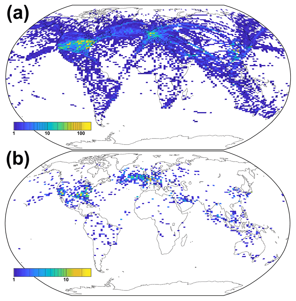
Figure 4Gridded map (0.5∘ latitude by 1.0∘ longitude) of the number of intercept points between the aircraft flight tracks above 5 km height and the ground track of the CALIPSO satellite for February 2012 for (a) all atmospheric conditions and (b) the situations in which cirrus is present at flight level. The maximum time difference between the primary and secondary tracks is constrained to 30 min.
Using a global chorded data set allows us to apply the approach of Tesche et al. (2016) to link the effects of embedded contrails on individual aircraft to regions of both low and high air traffic density. The occurrence rate of intercept points identified from using the global flight inventory for February 2012 as primary data and the CALIPSO satellite ground track of the same month as secondary data input for TrackMatcher is shown in Fig. 4. TrackMatcher identifies a total of 77 635 intercepts between the CALIPSO ground track and the tracks of civil aircraft for a time delay of ±30 min (Fig. 4a).
Naturally, the largest number of intercepts are found where flight density and contrail coverage are highest (see, e.g., Fig. 1 in Duda et al., 2019). Nevertheless, there is also a considerable number of intercepts in regions of lower air traffic density. In particular, distinct connections, such as between Hawaii and the continents or between Australia and New Zealand, can clearly be identified in Fig. 4a. The number of cases is reduced to 5076 in Fig. 4b, as this data set includes the demand for the detection of a cirrus clouds at flight level at each intercept. This decreases the number of identified intercepts by a factor of about 15. Using a global waypoint database is likely to yield a data set that is large enough to introduce sub-categories into the statistical analysis of the effect of embedded contrails on cirrus clouds.
The findings in Fig. 4 demonstrate that TrackMatcher can be applied to data sets of considerable size. However, parallel computation has not yet been achieved in TrackMatcher, with the exception of file reading with the CSV package. To achieve appreciable performance, the test month was split into four segments of about a week's length each. Accumulated file loading times are approximately 50 min for the flight data and ∼2.5 min for the satellite data. Overall, 2.25 ×10⁶ flights were loaded and processed to be saved in a unified format from 121 GB of data. A total of 3.8×10⁶ satellite data points were extracted and processed from 89 GB of CALIOP cloud profile data. The combined processing time to compute intersections was 3 d, 9 h, and 22 min.
Such a large data set allows for a detailed analysis of the precision of TrackMatcher calculations. TrackMatcher stores several interpolation accuracy parameters to evaluate the results. Parameters include the time and spatial distance to the nearest observed primary and secondary track point and an indicator for the precision of the calculation. This indicator is not the result of an error propagation. Instead, TrackMatcher takes the calculated x0 value for the determined root in the distance function (Eq. 1) and calculates the corresponding y0 from the interpolated trajectories of the primary and secondary tracks. Using the haversine function (Eq. 12), TrackMatcher calculates the distance between both computations of the intercept points using either the primary or secondary data set. The distance between both computations is the indicator for the interpolation accuracy. This indicator only recognises the accuracy of the interpolation method and the calculation of the roots in the distance function. It does not consider any measurement errors in the track data.
Table 4Statistics on the interpolation accuracy indicator and the spatial and temporal distances of the calculated intersection to the nearest measured track point of the primary or secondary data set for the run using data of February 2012 by the DOT Volpe Center. The units for the interpolation accuracy indicator and distances are in metres.

Table 4 shows the minimum, maximum, mean, and important quantiles for the interpolation accuracy indicator and the spatial and temporal distance to the nearest observed track point in the results of the TrackMatcher run for February 2012. Generally, CALIPSO satellite data of the secondary data set have a much greater density of track points, which is resembled by a median distance of about 1 km to the nearest measured track point compared to the median distance of 11 km for the primary flight data. Both data sets show some large data gaps, resulting in a maximum distance of 2615 and 4648 km of the computed intersection to the nearest observed track point of the primary and secondary data set, respectively. Due to the much greater velocity of the satellite compared to an aircraft, the maximum time difference to the nearest measured track point is only about 8 min for the secondary data compared to 6 h and 50 min for the primary data. Larger data gaps are more common in the primary data, which are represented by the fact of the mean in the range of the 68th percentile. For the secondary data, the mean corresponds to the 0.986 quantile. Hence, only about 1% of the track points can be found above the average of 1 km, and with a maximum distance of 4648 km, dominantly impacting the mean, whereas most distances between the calculated intersection and the nearest measured track point are significantly smaller.
TrackMatcher performs remarkably well, with most results being calculated with an interpolation accuracy of only a few metres. The median interpolation accuracy is 0.28 m, and the mean interpolation accuracy of 48 m is in the range of the 98th percentile. Then, 243 out of the 77 635 intersections or 0.3 % are computed with an interpolation accuracy larger than 1000 m, 1869 or 2.4 % are above 10 m, and 13 352 or 17.2 % are above 1 m of interpolation accuracy.
3.3 A year of cloud tracks over the Mediterranean
TrackMatcher is also useful for supporting aerosol–cloud interaction studies. Specifically, tracks of individual clouds, as inferred from time-resolved observations with an instrument aboard a geostationary satellite, should be matched with the tracks of polar-orbiting satellites that provide a highly detailed snapshot observation of the same clouds once during their lifetime. Here, cloud tracks in the region spanning from 16.5∘ W, 28.7∘ N to 34.3∘ E, 59.8∘ N during January to December of 2015, as identified in the CM SAF CLoud property dAtAset using SEVIRI (CLAAS-2) data set (Benas et al., 2017), following Seelig et al. (2021), have been used as primary input into TrackMatcher. The tracked clouds in this data set (i) are low-level clouds that (ii) formed in clear air and (iii) dissolved in clear air. All these clouds could be followed throughout the entirety of their lifetime. Clouds that originate from splitting or end as merged clouds are not tracked with the current methodology. Figure 5 shows the cloud tracks together with the identified intersections.
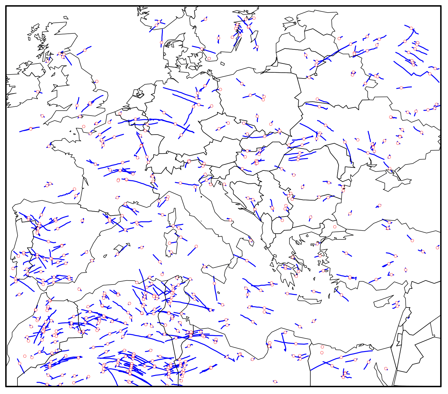
Figure 5Intercept points (red circles) between all cloud tracks (blue lines) and the CALIPSO ground track (not shown) identified in the region spanning from 16.5∘ W, 28.7∘ N to 34.3∘ E, 59.8∘ N during 2015.
In contrast to aircraft trajectories, the success rate of finding intersections in cloud tracks is significantly reduced. The main reason is that TrackMatcher compares sets of trajectories. Therefore, the centre points of a cloud trajectory have been matched to the satellite ground track. For clouds with a large horizontal extent, this means a high chance of the satellite monitoring the cloud, but not being identified by TrackMatcher, when the satellite does not pass the centre line of the cloud. A new method needs to be developed to compare an area or volume to a trajectory to increase the efficiency of the success rate in TrackMatcher. Another significant reason for the reduced number of matches is much shorter trajectories. With average cloud lifetimes of about 2 h (Pruppacher and Jaenicke, 1995), and with track points every 15 min, about eight track points per cloud can be expected. With the above-mentioned pre-conditions further reducing the primary data, the median cloud trajectory length is four track points. Overall, the data set consisted of over 1.7 ×10⁶ trajectories.
To increase the chances of finding intersections, the TrackMatcher run for cloud tracks allowed a maximum delay time of 5 h at the intersection between the overpass times of the primary and secondary trajectory. TrackMatcher was able to identify 2969 intersections. In total, 1527 intersections were within the default delay time of ±0.5 h. This corresponds to a success rate of 0.8 ‰ and 1.7 ‰ for standard and extended conditions, respectively.
3.4 Sensitivity study of key parameters
As indicated in Sect. 2.5 and by Table 1, parameters exist to compromise between the algorithm's performance and the accuracy of results. To investigate the influence of different settings, several sensitivity studies have been performed, where one parameter was varied from standard conditions. Table 5 summarises the computation time and identified intersections for the various studies. All sensitivity runs used flight track data from 1 January 2012 of the DOT Volpe data set, which contains almost 67 000 flight tracks. CALIOP profile data were used for the same day, except for the two runs investigating the use of CALIOP layer data.
Table 5Run times and the number of identified intersections for various sensitivity studies. The first column lists parameter settings. Float64 means all input data are loaded in double precision, and CLay means satellite data are loaded as layer data rather than profile data, with the additional condition of loading input in double precision in scenario CLay64. Parameters are applied during the calculation of intersections, unless otherwise indicated.
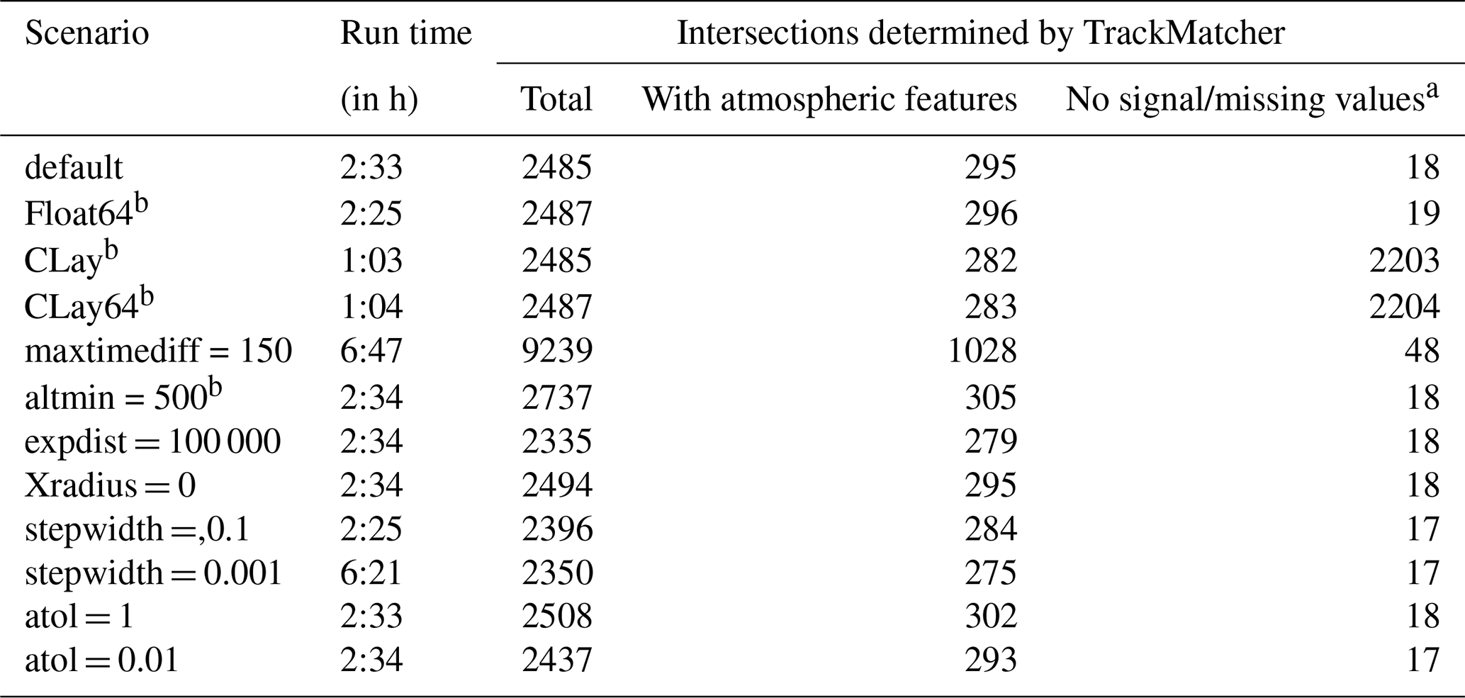
a Cloud layer data only recognise atmospheric features and do not distinguish between clear-sky conditions and no signal. Any non-featured values are treated as missing in TrackMatcher. b Parameter is applied during loading of input data.
Under default conditions, TrackMatcher finds 2485 intersections in 2:33 h. In total, 295 intersections include conditions other than clear sky or a missing signal. Most of the sensitivity runs using cloud profile data show a similar run time and similar success rates. Exceptions are the run with an increased maximum delay time between the primary and secondary trajectory overpass at the intersection that found 3.7 times more intersections and the run with a finer-resolved interpolation step width. Both cases see a massive increase in computation time to 6:47 h and 6:21 h for varying the maxtimediff and stepwidth parameter, respectively. The increase in computation time for increasing the maximum time difference can be explained by an increase in intercept finds to 9239. Surprisingly, the finer-resolved interpolation step width results in fewer identified intersections (2350). In essence, handing too many and too finely resolved data points to the IntervalRootFinding package results in a performance loss in terms of run time and sometimes even algorithm success.
Using cloud layer data instead of cloud profile data decreases computation times by a factor of 2.5. The same number of intersections are found; however, meteorological conditions are not always correctly identified (282 finds under non-clear conditions compared to 295 using cloud profile data). Moreover, it is not possible to distinguish data without meteorological features using layer data. Cloud profile data hold additional information such as clear-sky conditions or no lidar signal. On the other hand, using cloud layer data results in significantly reduced file sizes of the stored output (63.8 MB for layer data compared to 992.5 MB for profile data). In rare cases, the floating point precision of the input data can have an effect on the results, and two additional intersections are found by TrackMatcher when using double precision. While computation times are not affected by the floating point precision, switching to double precision increases the size of the output files, with negligible effects on the quality of the results. This effect is only seen for cloud profile data, where file sizes of saved output increased from 992.5 MB to 1.47 GB. File sizes for cloud layer data were almost identical (63.8 MB compared to 66.2 MB).
The number of false duplicate intersection identification can be inferred from the TrackMatcher run by setting the Xradius parameter to zero. Intersections increase to 2494; hence, nine duplicate intersections are falsely determined. Currently, TrackMatcher saves all intersections regardless of the distance to the nearest track point. Data can be filtered in a post-analysis, as the distance to the nearest track point is saved in the accuracy field of the Intersection struct. Furthermore, data could be filtered by the interpolation accuracy. Limiting the maximum distance to the nearest observed track point to 100 km decreases the determined intersections to 2335. The maximum interpolation accuracy indicator of 5598.8 m is identical to the base scenario, and the median interpolation accuracy of 0.28 m and mean interpolation accuracy of about 8 m are similar. Hence, inaccuracies in the computations are most likely not the result of the PCHIP method, even for track data with large gaps. Other factors influencing the precision of the results could be sharp bends in the trajectories or inaccuracies in the track data, leading to discontinuities.
This paper presents a tool for finding intercept points between tracks of geographical coordinates, i.e. data sets consisting of at least time, latitude, and longitude. The main principles of the methodology consist of (i) interpolating the primary and secondary tracks with a piecewise cubic Hermite interpolating polynomial and (ii) finding the minimum norm between the different track point coordinate pairs. The universal design of TrackMatcher allows the application of the tool to a wide range of scenarios, such as matching tracks from ships, aircraft, clouds, satellites, and in fact any other moving object with known track data.
Here, the tool is applied to find intercept points between flight tracks of individual aircraft and satellite ground tracks and between tracks of individual clouds and satellite ground tracks. Potential applications of the TrackMatcher tool in atmospheric science include the identification of intercept points between the tracks of research aircraft and the tracks of clouds or trajectories of air parcels from dispersion modelling. TrackMatcher will also prove useful in research fields outside the atmospheric sciences whenever data collected along different spatial pathways need to be collated with an objective and reproducible methodology.
However, current studies have also shown the limitations of TrackMatcher. Identification of intercept points matching cloud data with other trajectories can be improved with the development of an algorithm comparing trajectories and areas or volumes. Further development will also focus on performance improvements, e.g. by enabling distributed runs or parallel computation.
The TrackMatcher package is available at https://github.com/LIM-AeroCloud/TrackMatcher.jl (last access: 12 October 2022; https://doi.org/10.5281/zenodo.6193048, Bräuer, 2022a) under the GNU General Public License v3.0 or higher. Routines concerning the interpolation of track data with the PCHIP method are available in a separate package at https://github.com/LIM-AeroCloud/PCHIP.jl (last access: 12 October 2022; https://doi.org/10.5281/zenodo.6193059, Bräuer, 2022b) under the same licence.
All spaceborne lidar data used in this study are openly available, e.g. through the ICARE Data and Services Center at https://www.icare.univ-lille.fr/ (last access: 17 October 2022). Examples of flight track data are provided in the ESM.
The supplement related to this article is available online at: https://doi.org/10.5194/gmd-15-7557-2022-supplement.
TrackMatcher is based on an idea by MT and PB. The code development was lead by PB. Both authors contributed equally to the processing and interpretation of the data and the preparation of the paper.
The contact author has declared that neither of the authors has any competing interests.
Publisher's note: Copernicus Publications remains neutral with regard to jurisdictional claims in published maps and institutional affiliations.
The authors thank Torsten Seelig and Felix Müller, for providing the cloud trajectories used in the third application example. We thank Gregg G. Fleming, of the Volpe Center, for providing the aircraft waypoint data set for 2012.
This work has been supported by the Franco-German Fellowship Programme on Climate, Energy, and Earth System Research (Make Our Planet Great Again – German Research Initiative, MOPGA-GRI) of the German Academic Exchange Service (DAAD; grant no. 57429422), funded by the German Ministry of Education and Research.
This paper was edited by Simon Unterstrasser and reviewed by two anonymous referees.
Alfaro-Contreras, R., Zhang, J., Reid, J. S., and Christopher, S.: A study of 15-year aerosol optical thickness and direct shortwave aerosol radiative effect trends using MODIS, MISR, CALIOP and CERES, Atmos. Chem. Phys., 17, 13849–13868, https://doi.org/10.5194/acp-17-13849-2017, 2017. a
Benas, N., Finkensieper, S., Stengel, M., van Zadelhoff, G.-J., Hanschmann, T., Hollmann, R., and Meirink, J. F.: The MSG-SEVIRI-based cloud property data record CLAAS-2, Earth Syst. Sci. Data, 9, 415–434, https://doi.org/10.5194/essd-9-415-2017, 2017. a
Bezanson, J., Edelman, A., Karpinski, S., and Shah, V. B.: Julia: A Fresh Approach to Numerical Computing, SIAM Review, 59, 65–98, https://doi.org/10.1137/141000671, 2017. a
Brasseur, G. P., Gupta, M., Anderson, B. E., Balasubramanian, S., Barrett, S., Duda, D., Fleming, G., Forster, P. M., Fuglestvedt, J., Gettelman, A., Halthore, R. N., Jacob, S. D., Jacobson, M. Z., Khodayari, A., Liou, K.-N., Lund, M. T., Miake-Lye, R. C., Minnis, P., Olsen, S., Penner, J. E., Prinn, R., Schumann, U., Selkirk, H. B., Sokolov, A., Unger, N., Wolfe, P., Wong, H.-W., Wuebbles, D. W., Yi, B., Yang, P., and Zhou, C.: Impact of Aviation on Climate: FAA's Aviation Climate Change Research Initiative (ACCRI) Phase II, B. Am. Meteorol. Soc., 97, 561–583, https://doi.org/10.1175/BAMS-D-13-00089.1, 2016. a, b
Bräuer, P.: LIM-AeroCloud/TrackMatcher.jl: v0.5.3: Paper version for GMD, Zenodo [code], https://doi.org/10.5281/zenodo.6193048, 2022a. a
Bräuer, P.: LIM-LIM-AeroCloud/PCHIP.jl: v0.2.1, Zenodo [code], https://doi.org/10.5281/zenodo.6193059, 2022b. a
Christensen, M. W. and Stephens, G. L.: Microphysical and macrophysical responses of marine stratocumulus polluted by underlying ships: Evidence of cloud deepening, J. Geophys. Res.-Atmos., 116, D03201, https://doi.org/10.1029/2010JD014638, 2011. a
Duda, D. P., Bedka, S. T., Minnis, P., Spangenberg, D., Khlopenkov, K., Chee, T., and Smith Jr., W. L.: Northern Hemisphere contrail properties derived from Terra and Aqua MODIS data for 2006 and 2012, Atmos. Chem. Phys., 19, 5313–5330, https://doi.org/10.5194/acp-19-5313-2019, 2019. a, b
Fritsch, F. N. and Carlson, R. E.: Monotone Piecewise Cubic Interpolation, SIAM J. Numer. Anal., 17, 238–246, https://doi.org/10.1137/0717021, 1980. a
Iwabuchi, H., Yang, P., Liou, K. N., and Minnis, P.: Physical and optical properties of persistent contrails: Climatology and interpretation, J. Geophys. Res.-Atmos., 117, D06215, https://doi.org/10.1029/2011JD017020, 2012. a
Kahaner, D., Moler, C., and Nash, S.: Numerical Methods and Software, Prentice-Hall, Inc., Upper Saddle River, NJ, USA, 1989. a
Kato, S., Rose, F. G., Sun-Mack, S., Miller, W. F., Chen, Y., Rutan, D. A., Stephens, G. L., Loeb, N. G., Minnis, P., Wielicki, B. A., Winker, D. M., Charlock, T. P., Stackhouse, P. W., Xu, K. M., and Collins, W. D.: Improvements of top-of-atmosphere and surface irradiance computations with CALIPSO-, CloudSat-, and MODIS-derived cloud and aerosol properties, J. Geophys. Res.-Atmos., 116, 1–21, https://doi.org/10.1029/2011JD016050, 2011. a
Lee, D. S., Fahey, D. W., Skowron, A., Allen, M. R., Burkhardt, U., Chen, Q., Doherty, S. J., Freeman, S., Forster, P. M., Fuglestvedt, J., Gettelman, A., De León, R. R., Lim, L. L., Lund, M. T., Millar, R. J., Owen, B., Penner, J. E., Pitari, G., Prather, M. J., Sausen, R., and Wilcox, L. J.: The contribution of global aviation to anthropogenic climate forcing for 2000 to 2018, Atmos. Environ., 244, 117834, https://doi.org/10.1016/j.atmosenv.2020.117834, 2021. a
Pappalardo, G., Wandinger, U., Mona, L., Hiebsch, A., Mattis, I., Amodeo, A., Ansmann, A., Seifert, P., Linné, H., Apituley, A., Arboledas, L. A., Balis, D., Chaikovsky, A., D'Amico, G., De Tomasi, F., Freudenthaler, V., Giannakaki, E., Giunta, A., Grigorov, I., Iarlori, M., Madonna, F., Mamouri, R. E., Nasti, L., Papayannis, A., Pietruczuk, A., Pujadas, M., Rizi, V., Rocadenbosch, F., Russo, F., Schnell, F., Spinelli, N., Wang, X., and Wiegner, M.: EARLINET correlative measurements for CALIPSO: First intercomparison results, J. Geophys. Res.-Atmos., 115, 1–21, https://doi.org/10.1029/2009JD012147, 2010. a
Pruppacher, H. R. and Jaenicke, R.: The processing of water-vapor and aerosols by atmospheric clouds, a global estimate, Atmos. Res., 38, 283–295, https://doi.org/10.1016/0169-8095(94)00098-X, 1995. a
Quaas, J., Arola, A., Cairns, B., Christensen, M., Deneke, H., Ekman, A. M. L., Feingold, G., Fridlind, A., Gryspeerdt, E., Hasekamp, O., Li, Z., Lipponen, A., Ma, P.-L., Mülmenstädt, J., Nenes, A., Penner, J. E., Rosenfeld, D., Schrödner, R., Sinclair, K., Sourdeval, O., Stier, P., Tesche, M., van Diedenhoven, B., and Wendisch, M.: Constraining the Twomey effect from satellite observations: issues and perspectives, Atmos. Chem. Phys., 20, 15079–15099, https://doi.org/10.5194/acp-20-15079-2020, 2020. a
Redemann, J., Vaughan, M. A., Zhang, Q., Shinozuka, Y., Russell, P. B., Livingston, J. M., Kacenelenbogen, M., and Remer, L. A.: The comparison of MODIS-Aqua (C5) and CALIOP (V2 & V3) aerosol optical depth, Atmos. Chem. Phys., 12, 3025–3043, https://doi.org/10.5194/acp-12-3025-2012, 2012. a
Seelig, T., Deneke, H., Quaas, J., and Tesche, M.: Life cycle of shallow marine cumulus clouds from geostationary satellite observations, J. Geophys. Res.-Atmos., 126, e2021JD035577, https://doi.org/10.1029/2021JD035577, 2021. a, b, c
Stephens, G. L., Vane, D. G., Boain, R. J., Mace, G. G., Sassen, K., Wang, Z., Illingworth, A. J., O'connor, E. J., Rossow, W. B., Durden, S. L., Miller, S. D., Austin, R. T., Benedetti, A., Mitrescu, C., and Team, C. S.: THE CLOUDSAT MISSION AND THE A-TRAIN: A New Dimension of Space-Based Observations of Clouds and Precipitation, B. Am. Meteorol. Soc., 83, 1771–1790, https://doi.org/10.1175/BAMS-83-12-1771, 2002. a
Sun-Mack, S., Minnis, P., Chen, Y., Gibson, S., Yi, Y., Trepte, Q., Wielicki, B., Kato, S., Winker, D., Stephens, G., and Partain, P.: Integrated cloud-aerosol-radiation product using CERES, MODIS, CALIPSO, and CloudSat data, in: Remote Sensing of Clouds and the Atmosphere XII, edited by: Comerón, A., Picard, R. H., Schäfer, K., Slusser, J. R., and Amodeo, A., International Society for Optics and Photonics, SPIE, 6745, 277–287, https://doi.org/10.1117/12.737903, 2007. a
Tesche, M., Wandinger, U., Ansmann, A., Althausen, D., M\”uller, D., and Omar, A. H.: Ground-based validation of CALIPSO observations of dust and smoke in the Cape Verde region, J. Geophys. Res.-Atmos., 118, 2889–2902, https://doi.org/10.1002/jgrd.50248, 2013. a, b
Tesche, M., Zieger, P., Rastak, N., Charlson, R. J., Glantz, P., Tunved, P., and Hansson, H.-C.: Reconciling aerosol light extinction measurements from spaceborne lidar observations and in situ measurements in the Arctic, Atmos. Chem. Phys., 14, 7869–7882, https://doi.org/10.5194/acp-14-7869-2014, 2014. a
Tesche, M., Achtert, P., Glantz, P., and Noone, K. J.: Aviation effects on already-existing cirrus clouds, Nat. Commun., 7, 12016, https://doi.org/10.1038/ncomms12016, 2016. a, b, c, d, e, f, g, h, i, j, k, l, m, n, o, p, q, r, s, t, u, v
Turley, R. S.: Cubic Interpolation with Irregularly-Spaced Points in Julia 1.0, https://scholarsarchive.byu.edu/facpub/2177 (last access: 12 October 2022), 2018. a
Winker, D. M., Vaughan, M. A., Omar, A., Hu, Y., Powell, K. A., Liu, Z., Hunt, W. H., and Young, S. A.: Overview of the CALIPSO Mission and CALIOP Data Processing Algorithms, J. Atmos. Ocean. Tech., 26, 2310–2323, https://doi.org/10.1175/2009JTECHA1281.1, 2009. a