the Creative Commons Attribution 4.0 License.
the Creative Commons Attribution 4.0 License.
 | 11 Oct 2022
Estimation of missing building height in OpenStreetMap data: a French case study using GeoClimate 0.0.1
Erwan Bocher
Elisabeth Le Saux Wiederhold
François Leconte
Valéry Masson
Information describing the elements of urban landscapes is required as input data to study numerous physical processes (e.g., climate, noise, air pollution). However, the accessibility and quality of urban data is heterogeneous across the world. As an example, a major open-source geographical data project (OpenStreetMap) demonstrates incomplete data regarding key urban properties such as building height. The present study implements and evaluates a statistical approach that models the missing values of building height in OpenStreetMap. A random forest method is applied to estimate building height based on a building’s closest environment. A total of 62 geographical indicators are calculated with the GeoClimate tool and used as independent variables. A training dataset of 14 French communes is selected, and the reference building height is provided by the BDTopo IGN. An optimized random forest algorithm is proposed, and outputs are compared with an evaluation dataset. At building scale for all cities, at least 50 % of the buildings have their height estimated with an error of less than 4 m (the cities' median building heights range from 4.5 to 18 m). Two communes (Paris and Meudon) demonstrate building height results that deviate from the main trend due to their specific urban fabrics. Putting aside these two communes, when building height is averaged at a regular grid scale (100 m×100 m), the median absolute error is 1.6 m, and at least 75 % of the cells of any city have an error lower than 3.2 m. This level of magnitude is quite reasonable when compared to the accuracy of the reference data (at least 50 % of the buildings have a height uncertainty equal to 5 m). This work offers insights about the estimation of missing urban data using statistical methods and contributes to the use of open-source datasets based on open-source software. The software used to produce the data is freely available at https://doi.org/10.5281/zenodo.6372337 (Bocher et al., 2021b), and the dataset can be freely accessed at https://doi.org/10.5281/zenodo.6855063 (Bernard et al., 2021).
- Article
(8043 KB) - Full-text XML
- BibTeX
- EndNote


The topography – defined as the spatial distribution of natural and artificial land use features – has a significant influence on the microclimate. This is clearly visible in urban areas, where the great heterogeneity of forms, materials and land uses induces high variability in temperature, wind speed and humidity (Oke, 2002). Thus an in-depth knowledge about the topography of a location would lead to a better understanding and more accurate modeling of its climate as well as of other physical processes, such as noise propagation and air pollution (Tang and Wang, 2007; Bocher et al., 2019).
There are currently no standard geographical data to study the urban climate worldwide. However, urban data tend to increase under both closed license and open-source. A key open-source data approach is the OpenStreetMap (OSM)1 project. Data from the latter have several features: they are expected to be available worldwide, and the most important objects needed for urban climate studies (building footprints, isolated tree locations, water, vegetation and impervious patches) are available, well located and described using a great diversity of tags (Mocnik et al., 2017). Moreover, OSM has a free tagging system that allows users to improve the current tags (key, value) with their own information (an OSM user can describe a building object with the tags such as the following: “building”=“house”, “height”=“10”, “building:levels”:“2”).
However, information concerning building height is not available worldwide, neither in OSM nor in any other database (Masson et al., 2020). Lao et al. (2018) reported that less than 3 % of buildings globally have a height value, and less than 4 % have a number-of-levels value. For the city of Paris (where this information is known to be quite well informed), the values are only 0.1 % and 51.2 %, respectively. This is a major shortcoming, since the urban climate is often characterized by spatial indicators based on the third dimension:
-
The sky view factor (SVF), which is calculated according to terrain level variations, building and tree locations and heights, is related to effective albedo (Bernabé et al., 2015) and is strongly correlated to temperature (Lindberg, 2007) and wind speed (Johansson et al., 2016).
-
The building height variability within an area affects the vertical and horizontal wind speed (Hanna and Britter, 2010).
-
The roughness length of an area, often calculated using facade density, is used to estimate the wind speed vertical profile of the urban canopy (Hanna and Britter, 2010).
The objective of this study is to develop a method to estimate the height of a building from its topographical context using only data available in OSM. Modeling building footprints and their height value has been largely covered by remote sensing. It can cover large areas at once quite efficiently, and the resulting datasets can be updated quite easily with a repetitive coverage. Different techniques for building height extraction have been developed based on photogrammetric processing (Fradkin et al., 1999; Zeng et al., 2014), analysis of point clouds from airborne light detection and ranging (Sohn et al., 2008; Shan and Toth, 2018), shadow detection (Song et al., 2013; Shao et al., 2011) and, more recently, a deep learning approach (Cao and Huang, 2021).
In the meantime, the recent and global movement regarding open data – specifically for vector topographic databases such as OSM – offers new opportunities to estimate building height. The geography of a territory and the pattern of the topographic elements are criteria that can be used as a proxy to identify the urban forms and therefore the distribution of building heights. Biljecki et al. (2017) have used building footprints and their corresponding attributes to derive building heights for the city of Rotterdam, the Netherlands. They have tested several random forest models using building properties characterizing its geometry footprint (size, shape and number of neighbors), other attributes (use, age and number of levels), and information concerning the inhabitants (the number and their levels of income) as independent variables. Milojevic-Dupont et al. (2020) have proposed a random forest approach to estimate building height using 152 features. These independent variables are related to buildings (e.g., footprint geometry), streets (e.g., closest street, closest intersection), street-based blocks (e.g., number of blocks in a given radius) and cities (e.g., total city area). For the base case, the training dataset includes the building heights of the Netherlands, the region of Friuli Venezia Giulia in Italy and five French urban areas, and the validation dataset includes the building heights of the state of Brandenburg in Germany.
A major limitation of these studies is the obstacle of reproducibility for experts and practitioners. Indeed, the algorithms are not fully available. Moreover, input datasets require many preprocessing steps, since the format and the access differ between city models (e.g., French 3D city models in Milojevic-Dupont et al., 2020). The method presented in the next sections uses a random forest approach and can be easily reproduced using the GeoClimate software without any preprocessing steps, since it is based exclusively on OSM data. The main spatial indicators used by the urban climate communities are also calculated using reference and estimated building heights. Compared to each other, they provide urban climate researchers with a good level of magnitude in terms of the impact of the estimated height on these indicators. OSM data do not contain as much detailed information about buildings as that seen in Biljecki et al. (2017) (number of levels, age, number of inhabitants), but other information describing the environment of the buildings will be used (roads, vegetation, rail, etc.).
In order to make OSM data available to urban climate researchers, the GeoClimate tool has been developed (E. Bocher et al., 2021; Bocher et al., 2021a). It is an easy way (i) to download most of the information needed for urban climate studies, (ii) to estimate building height from the topographical context, and (iii) to calculate spatial indicators (such as SVF, building height variability or roughness length) that are useful as input for parametric climate models. This paper focuses on the second item, namely how to estimate building height in OSM when the information is missing. First, the data and the methodology used to estimate the building height are presented (Sect. 2), and second, the accuracy of these estimations is analyzed (Sect. 3).
This study presents a method to estimate values of building height when the information is missing in OSM. The height of a building is determined according to a regression-based statistical model (e.g., random forest model) using a set of spatial indicators – including the building's shape, the building's relation to its neighbors, and the organization and morphology of the building's environment – as independent variables. The true building height values come from the BDTopo V2.2 (BDT) provided by the French National Geographic Institute (IGN). These values are defined as reference height. Two datasets have been considered for this study, namely a training dataset to build the random forest algorithm and a validation dataset to compare the outputs of the optimized random forest algorithm with reference heights. The overall methodology is illustrated in Fig. 1 and consists of the following steps:
-
Building characterization. Each building and its environment (limited to the topographical spatial units (TSU) it belongs to – defined in Sect. 2.2.1) are characterized by spatial indicators (building area, number of buildings neighbors, vegetation fraction, etc.). These indicators are the independent variables of the statistical model.
-
Building height attribution. The reference building heights (BDT building heights) are attributed to each OSM building according to their footprints. The resulting height in the OSM dataset is the dependent variable of the statistical model.
-
Statistical analysis. The random forest model is built based on the training dataset. In this step, parameters that maximize the performance of the random forest model are identified.
-
Performance evaluation. Outputs of the optimized random forest model are evaluated against the reference heights of the validation dataset.
Each step is described further in Sect. 2.2.
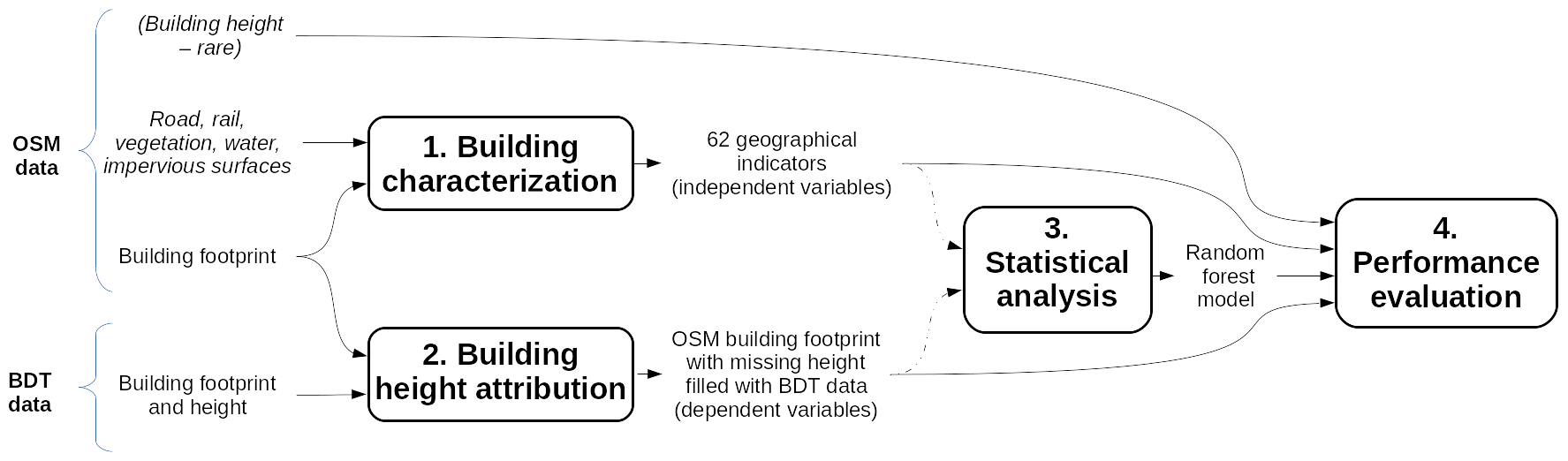
Figure 1Overall methodology – the use of dashed arrows means that only the training dataset is used.
2.1 Study area
Building organization and height may differ a lot throughout the world, limiting the ability to model the height of a building based on the characteristics of its environment. Thus, although the method can be used to estimate the height of any building in the world, the application area of this preliminary work is limited to the French territory. The training and evaluation areas are selected to cover
-
all types of communes (from small villages to large conurbations)
-
a large part of France (Fig. 2), increasing the probability of having cultural and/or historical differences inducing urbanistic heterogeneities
-
the main geographical constraints for construction (nearby mountains – Annecy, La Thuile, Corbonod – and nearby sea – La Rochelle).
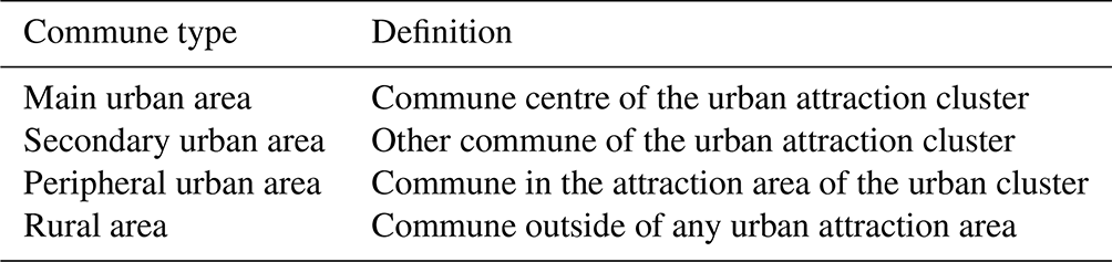
To fulfill the first need, the communes have been chosen to cover each of the four French commune types defined by the French National Institute of Statistics and Economic Studies (INSEE, 2020): main urban area, secondary urban area, peripheral urban area, rural area. According to the French 2020 census data, the types are defined based on the following commune characteristics: number of inhabitants, density of population, number of employees, and population flow between households and workplaces. They are used to define the urban attraction cluster. The definitions of each type are given in Table 1.
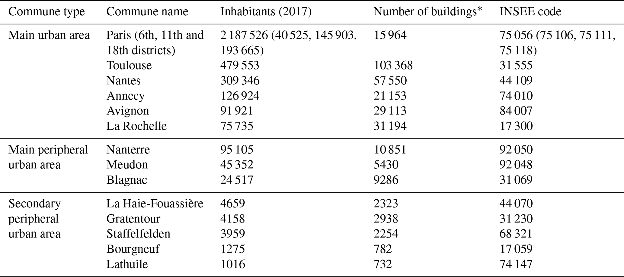
The training and the evaluation datasets contain 14 and 8 communes, respectively. The location of each commune is shown Fig. 2, while further information concerning each territory is in given Tables 2 and 3 (for training and evaluation datasets, respectively).
Table 2Information and statistics about the training dataset.
* Only buildings that have a height value higher than 3 m in the BDT (cf. Sect. 2.2.2) have been conserved for this evaluation.
Table 3Information and statistics about the validation dataset.
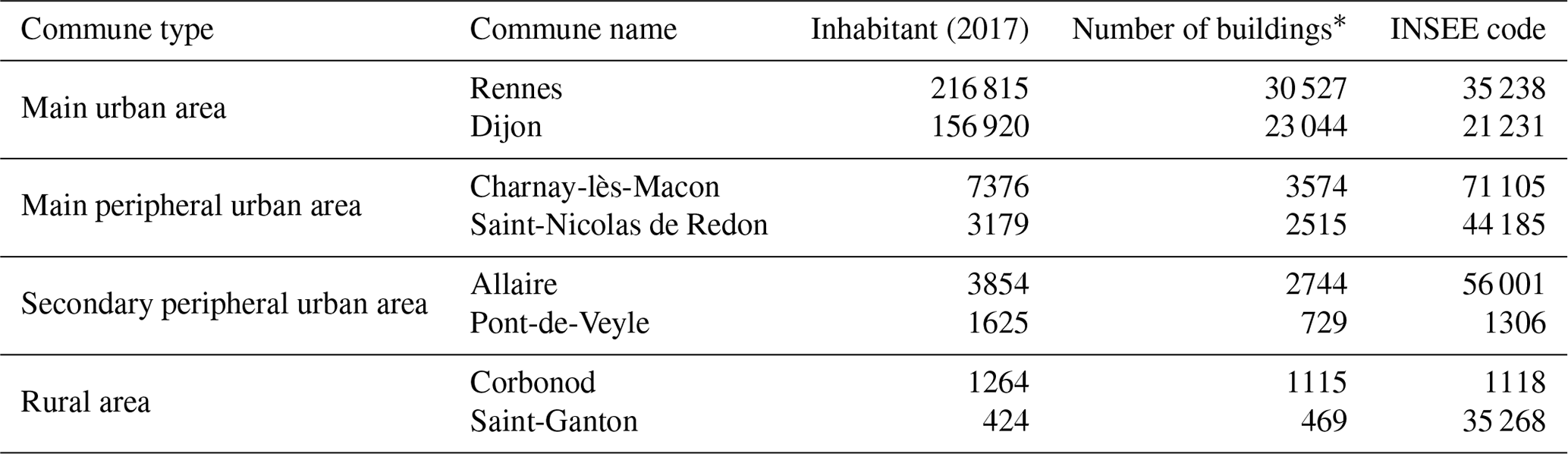
* Only buildings that have a height value higher than 3 m in the BDT (cf Sect. 2.2.2) have been conserved for this evaluation.
2.2 Methodology
2.2.1 Building characterization
Data from OSM are used to characterize the building and its environment: building footprint, vegetation footprint and type, water footprint, impervious footprint, rail and road footprint. The free and open-source GeoClimate software (E. Bocher et al., 2021; Bocher et al., 2021a) is used to compute the spatial indicators at three different scales:
-
building scale
-
block scale, defined as the aggregation of all buildings touching each other
-
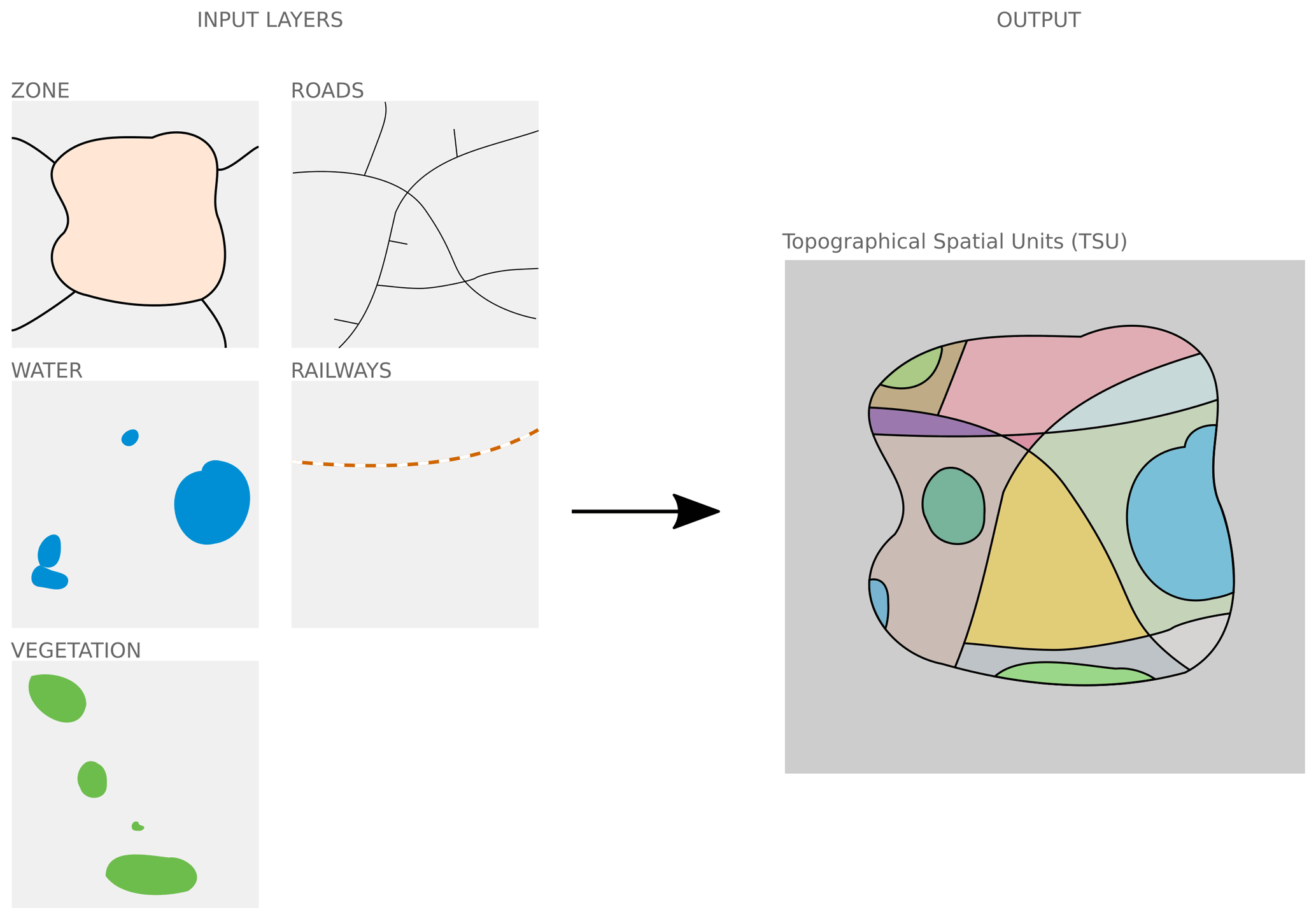
topographical spatial unit (TSU) scale, defined according to the central lines of roads and rails, commune boundaries, and water and vegetation boundaries when their area is higher than 2500 and 10 000 m2, respectively (Fig. 3).
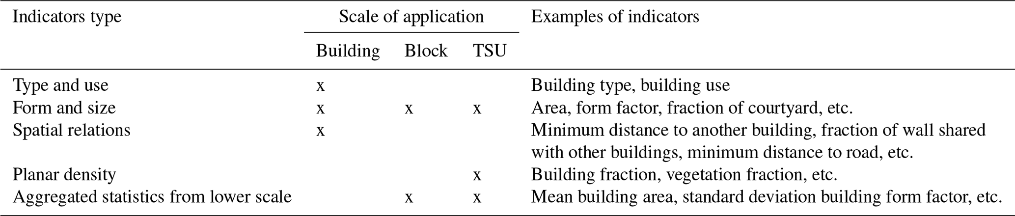
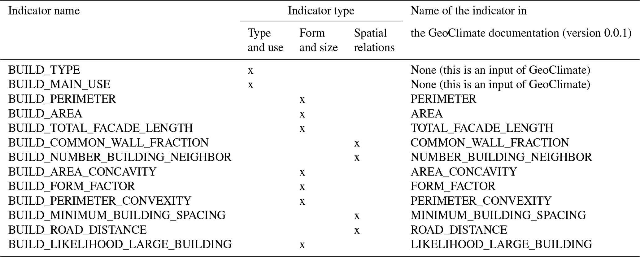
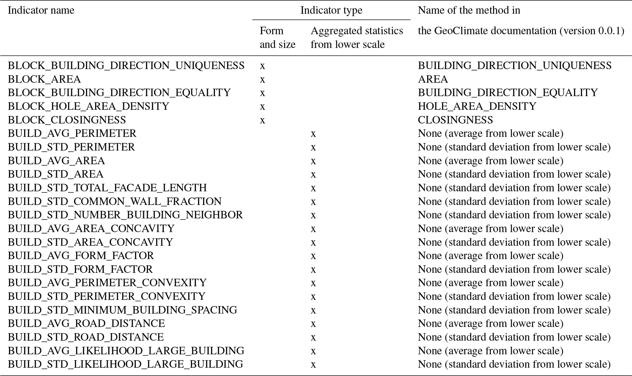
Each building is described by a total of 62 spatial indicators (note that all characteristics are calculated in two dimensions only, since most OSM data do not have height information). Four types of indicators are used (see Table 4) and the list of all indicators is given in Appendix A. Indicator values calculated at block and TSU scales are then attributed to each building (a building within a given block or TSU embeds the indicator values of the block and the TSU it belongs to).
Table 4Types of spatial indicators used to define the main characteristics of each unit scale.
2.2.2 Reference building heights attribution
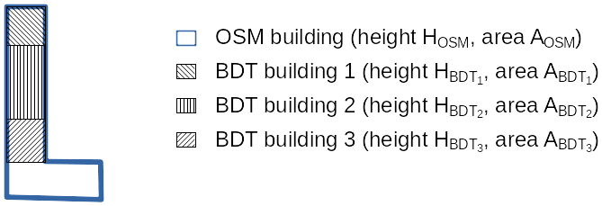
In order to train and evaluate the statistical model, a reference height used as a true value should be assigned to each OSM building. Most of the OSM buildings do not have any information concerning their height. The few buildings with height information could have been considered as training and evaluation datasets; however, these buildings are sparse and not representative of common buildings (since most of them are filled out by OSM users because they are well-known buildings with specificities). Therefore, the training and evaluation datasets are created only with OSM buildings that have no height. The reference height is set using the BDT data. However, a single building in OSM may match with several buildings in the BDT (Fig. 4).
Thus, the height of an OSM building used as a reference (Hosm,true) is calculated from the height of all intersecting BDT buildings according to Eq. (1). This equation is applied for both the training and the validation datasets.
with Ai being the area of the intersection between an OSM building and a BDT building i, and being the height of the BDT building i intersecting the OSM building.
In the example presented in Fig. 4, if BDT building 1 is much taller than the others (BDT buildings 2 and 3), this information is lost (smoothed by the averaging) and could then lead to a bias in the learning process. To keep track of this potential bias, a simple index is proposed to characterize the proportion of the intersection between a BDT building and an OSM building. This index, called uniqueness value (UV), is defined in Eq. (2):
The uniqueness value considers only the BDT building that demonstrates the largest intersection area with a given OSM building. The higher the UV, the more unique the BDT building intersecting the OSM building. UV is not impacted by the fraction of the OSM building shared with other BDT buildings. If only one BDT building overlaps only a small fraction of an OSM building, the uniqueness value will be 1.
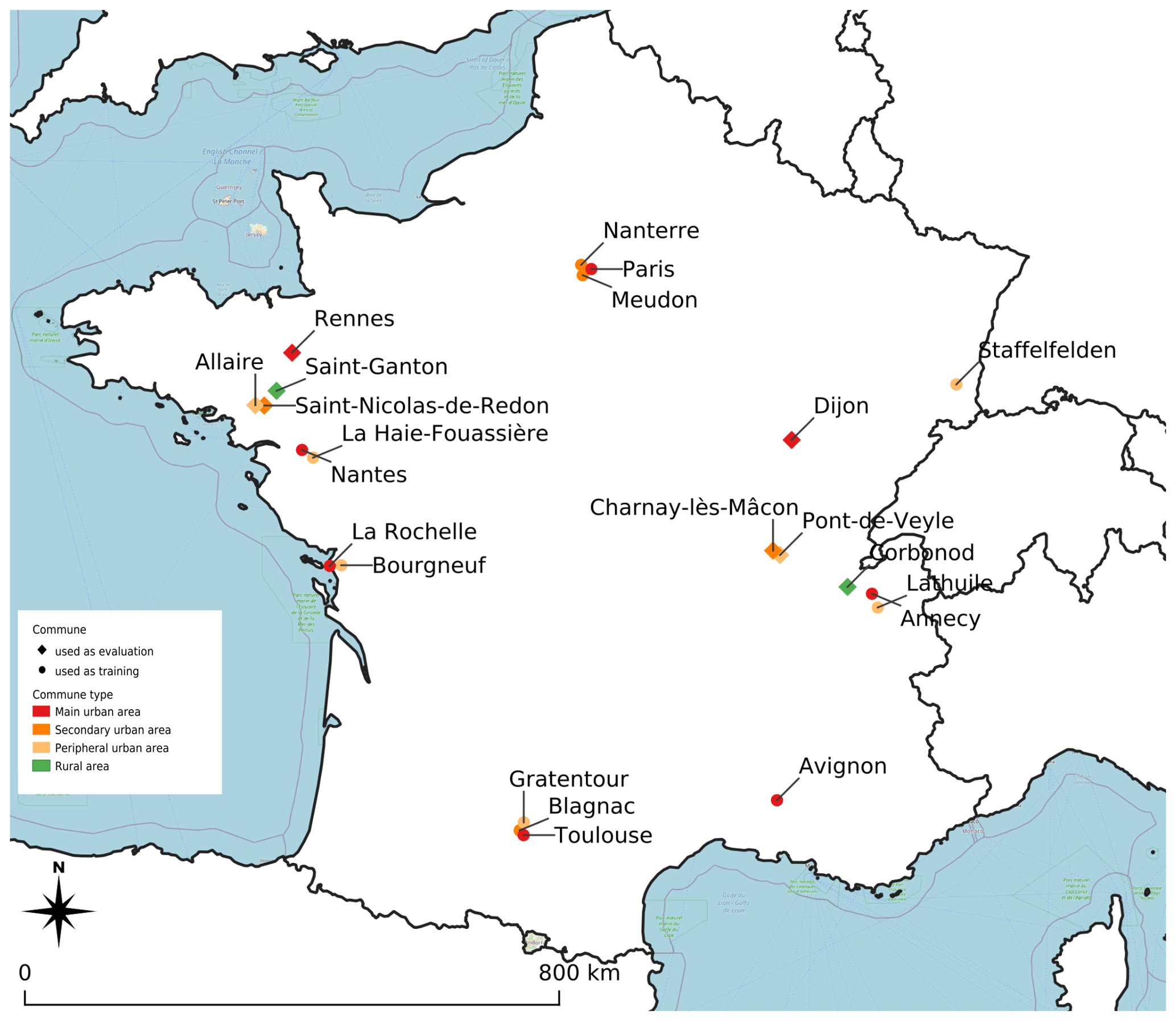
Figure 2Location of the 22 communes used as training or evaluation data. ©OpenStreetMap contributors 2021. Distributed under the Open Data Commons Open Database License (ODbL) v1.0.
2.2.3 Design and optimization of the random forest statistical model
For the statistical analysis, the OSM building height (reference height Hosm,true) is defined as the dependent variable, while spatial indicators are defined as independent variables. Only the training dataset (see Table 2) is used for this step. To obtain an optimal model, the methodology illustrated in Fig. 5 is applied.

Figure 5Method to train and optimize the random forest model. Only the training dataset is used at this step.
The random forest (RF) approach is chosen for several reasons: (i) it is simple to implement, (ii) it deals with quantitative and qualitative variables, and (iii) it is appropriate when using a large number of variables (Hastie et al., 2001). In order to limit overfitting and a high correlation between trees, all combinations of the following RF regressor parameters are investigated:
-
number of trees: 100, 350, 500, 650 (note that preliminary analysis showed lower accuracy when the number of trees was lower than 100 and no significant improvement when greater than 650);
-
minimum node size (minimum fraction of the sample used to create a new node): 0.0001 %, 0.001 %, 0.005 %, 0.01 % (the whole sample size includes 345 418 individuals – note that preliminary analysis showed decreasing performance over 0.01 %);
-
maximum variables per tree (maximum fraction of variables used in a tree): 20 %, 35 %, 50 % (of a total of 62 variables – note that preliminary analysis showed decreasing performance when the fraction was lower than 20 % and no significant improvement over 40 %);
-
maximum leaf nodes (maximum number of leaves in a tree): 300, 500, 800, 1100 (note that preliminary analysis showed no significant improvement over 1100 while increasing the complexity and thus potentially the overfitting).
For a default combination of 500 trees, 0.001 % minimum node size and 30 % maximum variables per tree, the effect of UV on the accuracy is studied, keeping only buildings having a UV above 30 %, 70 %, 90 % and 95 %.
A total of 70 % of the training data are randomly drawn to construct the RF. The accuracy is calculated using the remaining 30 % of the data. This process is performed 10 times for each combination Ci and uniqueness value UVi. The scikit-learn Python algorithm is used for this investigation.
The optimized combination Copt and uniqueness value UVopt leading to the lowest mean absolute error (MAE) are used to construct the final RF model used in GeoClimate. For this purpose, the entire training dataset is used as input for the Smile library algorithm (since GeoClimate is Java-based).
2.2.4 Performance evaluation
The optimized RF model obtained in the previous step is run over the eight communes of the validation dataset to calculate the missing height values of the OSM buildings. For each building, the heights estimated with the optimized RF model () are then compared to the reference height (HOSM,true). The model error Errmodel is defined for heights estimated by the random forest model:
The building height values filled out by the OSM users () are also compared to the reference height. If the user filled only the number of storeys, the building height is simply calculated by multiplying the storey number by 3 m. Even though the storey height may vary quite a lot between construction age and building type (see Biljecki et al., 2017 – Fig. 5), 3 m seems to be a reasonable value according to the one observed in the literature (ranging from 2.8 to 3.5 m – see Biljecki et al., 2017; Sect. 2.2.1). The user error Erruser is defined for heights filled by the users (Eq. 4).
In parametric urban climate models, parameters such as building height are aggregated within each square cell of a regular grid. Therefore, four indicators are calculated for a grid of 100 m width square: the mean building height and standard deviation, the roughness length (as defined by Hanna and Britter, 2010), and the SVF (as defined in Bernard et al., 2018).
The dataset produced by the methodology described in Sect. 2.2 can be freely downloaded at https://doi.org/10.5281/zenodo.6855063 (Bernard et al., 2021). In this section, cells that have no building with an estimated height are not considered for the statistical calculations.
3.1 Optimized configuration of random forest characteristics
Very little accuracy difference is observed between all combinations described in Sect. 2.2.3. For all studied configurations, the median RMSE ranges between 2.05 and 2.2 m. The minimum node size and the number of trees (when greater than 100) have the least significant impact on the accuracy. The highest accuracy is reached when the maximum variables per tree is 50 % and the maximum leaf nodes is 1100. Thus, the RF scenario chosen for GeoClimate has 350 trees, 40 % maximum variables per tree (based on previous results showing little difference between 40 % and 50 %) to minimize the correlation between trees, 0.01 % minimum node size, and 1100 maximum leaf node to minimize the potential of overfitting (Hastie et al., 2001). Since the maximum tree depth obtained in Python for this configuration is 33, this value is also applied to the GeoClimate RF algorithm. The uniqueness value has an unexpected effect on the accuracy: the MAE decreases when UV value increases up to 70 % and increases for UV values above 90 %, while it could be expected to continue decreasing. However, the difference is slight (0.05 m, 2.5 %) and may be explained by the size of the sample, which is larger (+23 %) for the 70 % scenario than for the 95 % (having 345 418 and 281 081 individuals, respectively). Therefore, the data used to train the GeoClimate model are created with UV =70 %.
3.2 General building height accuracy
For all cities, more than 50 % of the buildings have an estimated height within a ±3.97 m (3.22 m if the 18th district of Paris is excluded) interval around the true building height (Fig. 6a). At cell scale (Fig. 6b), the same statistic is ±4.61 m (2.74 m if the 18th district of Paris is excluded). If cities demonstrating a specific behavior are not considered (Paris and Meudon), the median absolute error at cell scale is always lower than 1.6 m, and 75 % of the buildings or cells of any city have an error lower than 3.2 m. This error is equivalent to the floor height of one building and could appear quite high. However, it seems quite reasonable when compared with the accuracy of the reference data (i.e., the height uncertainty of more than half of the BDT dataset is ±5 m). Note that we have tested a previous version of the model (independent variables have been updated since then) on several cities far from the ones presented in this manuscript, and the error was almost similar.

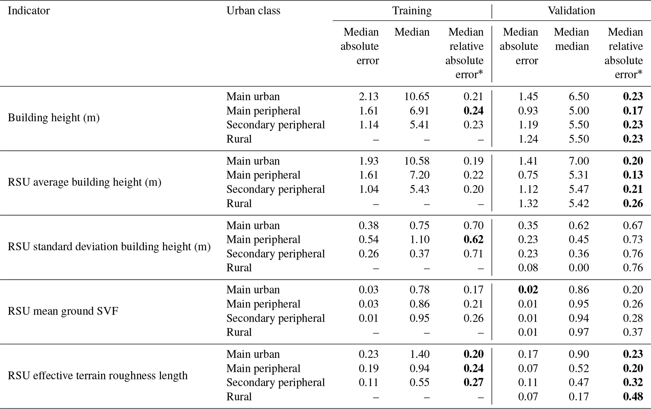
Figure 6Median absolute error versus median true value for (a) building height, (b) RSU average building height, (c) RSU standard deviation building height, (d) RSU mean ground sky view factor, and (e) RSU effective terrain roughness length. The cross and the dot are the medians, while the whiskers are the first and third quartiles.
Table 5Summary of the main statistics for each combination of {indicator, commune type, dataset type}. Bold values are the ones described in the text.
* Contrarily to the other indicators, the reference value used for MRAE is not the SVF of the grid cell but 1-SVF of the grid cell.
Surprisingly, the worst results are obtained with communes belonging to the training dataset (the median relative absolute error – MRAE – is 24 % for main peripheral communes – Table 5). Overall, there is almost no accuracy decrease when the model is applied to the validation dataset (Fig. 6). No city type shows a specific pattern; even the rural areas, which are not included in the training dataset, do not show a clearly higher error (MRAE =23 %) than the overall trend (MRAE =22 % on average). However, a specific behavior is observed for the city of Meudon and for the 18th district of Paris, which have a higher error than the main trend (Fig. 6b). A part of the explanation can be found in their uncommon urban fabrics, which makes them more difficult to estimate by the RF model:
-
Meudon has quite a low median height (Fig. 6b) while also having a high building height variability within a 100 m square (Fig. 6c);
-
the 18th district of Paris has the highest average building roof height at grid scale (Fig. 6b) but also the highest sky view factor of the three Parisian districts (Fig. 6d) even though it would be expected to have the lowest.
3.3 Accuracy of standard spatial indicators
The building height estimation is slightly improved when averaged at RSU scale (MRAE decreases from about 3 % for all communes types except for rural areas). The variability of height within a cell is very roughly calculated using the estimated height: for more than 50 % of the cells, the MRAE on the standard deviation of the building height is higher than 62 % (Table 5). This behavior is quite understandable, since the RF model smooths the values of the estimated height; it cannot reproduce entirely the complexity of the initial dataset. The roughness length MRAE is about 25 %. This error is slightly higher for secondary peripheral and rural communes (29.5 % and 48 %, respectively – Table 5), while Meudon and the 18th district of Paris show higher values than the MAE trend (Fig. 6e). The sky view factor is quite accurately calculated: more than 50 % of the cells have an absolute error lower or equal to 0.02 (Table 5). The effect of the building height error is probably limited, because the sky view factor is a 3-dimensional indicator: it also accounts for the horizontal footprint of the building, which is the same between the estimated and observed data.
3.4 Limitations of the model for high-rise buildings
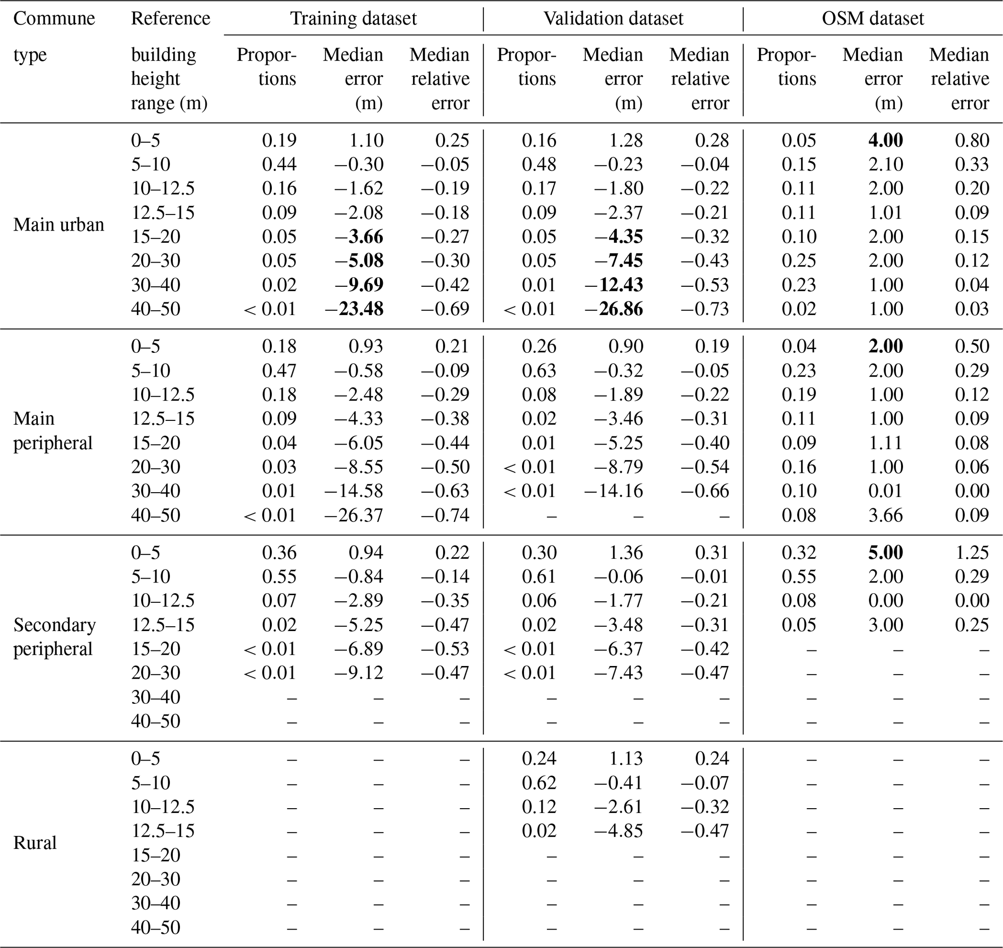
The accuracy differs a lot between low-rise and high-rise buildings. For all types of cities, the building height is often overestimated for buildings smaller than 5 m and often underestimated for the taller ones (Fig. 7). The bias for high-rise buildings can be quite high, but it does not affect the general accuracy of the model, since most of the buildings are low-rise (see Fig. 7: 80 % of the buildings are lower than 10 m – even in main cities). A better estimation of the high-rise buildings may be achieved using a training dataset containing an equal number of buildings for all levels. This would allow a better representation of the spatial heterogeneity of the third dimension. However, this would most probably affect the accuracy of the estimation for low-rise buildings. Indeed, in France, low-rise building are much more numerous than the high-rise ones.
As previously observed, there is almost no accuracy decrease between the training and the validation estimations, even for high buildings. Only a slight difference can be observed for main urban cities: above 15 m, the training dataset performs better than the validation one (almost 3 m difference – Table 6).
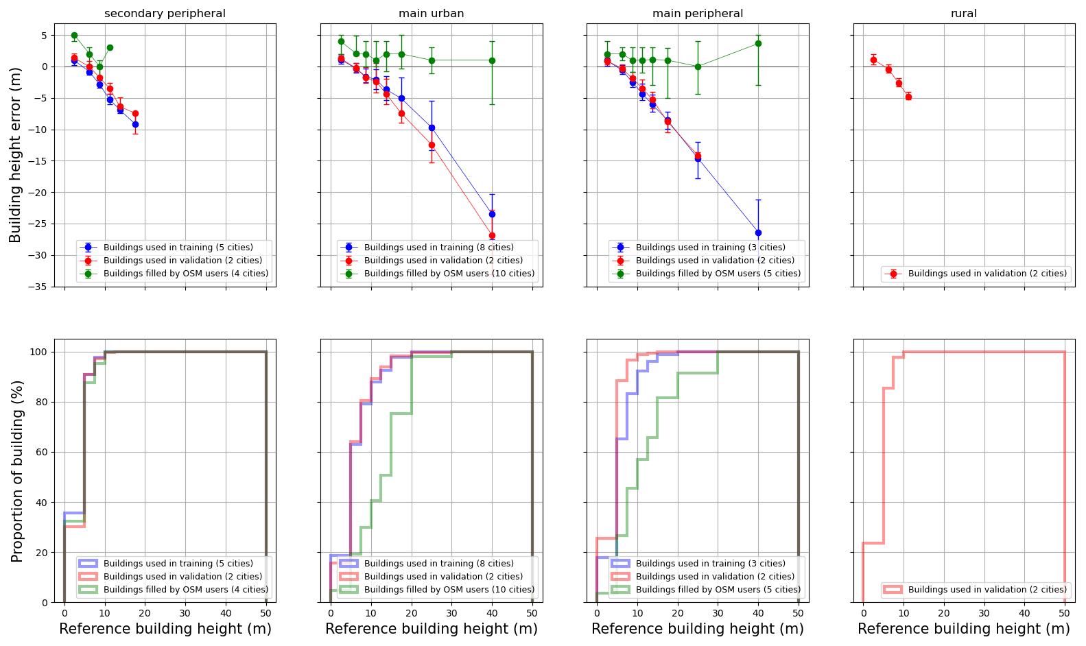
Figure 7On the top: building height errors (Errmodel and Erruser) versus reference building height (HOSM,true) for each type of city. The dots represent the median, while the whiskers are the 1st and 3rd quartiles. On the bottom: cumulated distribution of reference building height (HOSM,true) for each type of city. The intervals used for the reference building height (the abscissa) are based on the following values: 0, 5, 7.5, 10, 12.5, 15, 20, 30, 50 m (values above 50 m are not considered, since their number is negligible and they affect the reading).
Table 6Summary of the building height estimation error by commune type, building height range and dataset type.
This difference is attributed to the Paris buildings dataset: the two curves almost coincide if the latter is excluded. The reason is that Paris buildings are quite accurately calculated and represent a large part of the training dataset (43.2 % of the buildings higher than 15 m). The urban fabric (very dense block of buildings with courtyards) and the building heights are quite homogeneous in Paris, thus being well taken into account by the model. In most other cities, a large amount of the high-rise buildings are isolated buildings (see Fig. 8 for an example with the city of Nantes). These buildings probably have very little shape or environmental differences with smaller, isolated buildings and are probably less numerous. Therefore, most of these buildings are seen as low-rise by the model.

Figure 8Buildings taller than 15 m for which the height underestimation is higher than 30 %. © OpenStreetMap contributors 2021. Distributed under the Open Data Commons Open Database License (ODbL) v1.0.
It is interesting to notice that the buildings that already have a building height value in OSM (or at least a number-of-floors value) are, most of the time, slightly higher than the BDT ones (Fig. 7). This is the case for low-rise buildings (lower than 5 m – Table 6) in particular, and it may be explained by the fact that the BDT heights are taken at the lowest part of the roof. The OSM data can take into account the roof height, which is, most of the time, equal to zero for tall buildings but non-negligible for small buildings. The difference between height derived from OSM user filling and the reference data (BDT) is quite low for any building height. This result may be used to improve the model performance – when estimating the height of a given building, the random forest may take into account the height of a nearby building filled by an OSM user as an extra independent variable.
3.5 Spatial distribution of the building height at city scale
While most of the buildings higher than 15 m are underestimated, the model allows one to represent the spatial patterns of the third dimension well; at grid scale, the average building height maps of estimated and reference values look quite similar (Fig. 9; Appendix B for other cities). While the model smooths the values slightly, the city center, first ring and second ring are quite easily distinguishable. Note that this is not the case for cities that have a more homogeneous spatial distribution of the building height values (e.g., Annecy, which is constrained by the topography – see Fig. B1 in Appendix B).
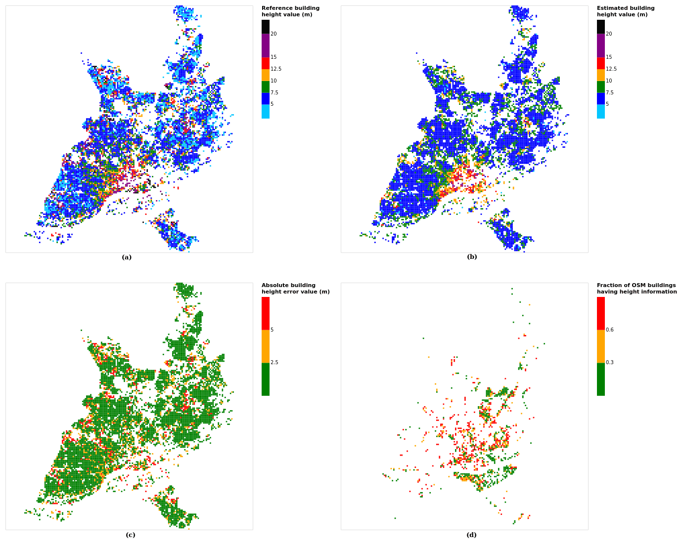
Figure 9Results for the city of Nantes at grid cell: (a) reference building height, (b) estimated building height, (c) absolute building height error, and (d) fraction of OSM buildings that have height information. For cases (a), (b) and (c), only cells that have buildings with at least 90 % of their buildings having no height value in OSM are displayed.
For most of the city pixels, the absolute error is under 2.5 m, and only a small proportion of cells have an error higher than 5 m (Fig. 9). This absolute error magnitude is within the accuracy of the reference building dataset. Indeed, according to the data supplier's (IGN) information (based on a sample of 7 299 422 buildings), 8.2 % of the buildings have an accuracy of 1 m, 13.5 % an accuracy of 2.5 m, and 68.8 % an accuracy of 5 m, while 9.5 % have no accuracy information.
There is a need for a world-wide database of morphological indicators that would be useful for many physical process interests (e.g., parametric urban climate models, noise modeling, urban planning). The GeoClimate tool aims to tackle this issue using the OpenStreetMap data. However, most of the OSM buildings do not have any information concerning their height, which is a crucial parameter for urban climate studies. A random forest model has been integrated within GeoClimate to estimate the height of a building based on spatial indicators describing its shape, its relations to other buildings and the 2D characteristics of its close environment.
This article presents the method for building and evaluating this model. The buildings from 14 French communes have been used to train the model, while the evaluation was based on 8 French communes. Attention was paid to having as many types of territories (based on the French definitions) in the samples as possible, including main urban, main peripheral, secondary peripheral and rural.
The random forest model was tuned according to four parameters: the number of trees (best 350), the minimum node size (best 0.01 %), the maximum variables per tree (best 40 %), and the maximum leaves per tree (best 1100). The reference heights used for the training of our OSM buildings were based on a dataset (French BDTopo – BDT) where buildings could not fit exactly with the OSM ones. Thus, the matching between each OSM building footprint and BDT building footprint has been quantified using the uniqueness value indicator. The latter equals 1 if only one building from the BDT was used to feed the OSM building height; it is otherwise lower than 1 and is best suited to the random forest model when values are higher than 0.7.
Two communes (Paris and Meudon) demonstrate a specific behavior within the analysis. Apart from these, the median absolute error at cell scale was always lower than 1.6 m, and 75 % of the buildings or cells of any city had an error lower than 3.2 m. This level of magnitude is similar to the BDT data used for the training: 68.8 % of the buildings heights demonstrated an uncertainty of 5 m.
Geographical indicators commonly used in urban climate studies have also been calculated at a 100 m grid cell according to the estimated building height. While the building height variability (standard deviation within a grid) is strongly affected by the building height estimation error (50 % of the cells have more than 50 % error in building height standard deviation value), the roughness length and sky view factor have a relative error of about 20 % for 50 % of the cells.
One of the major limitations of the model at the French scale is presented when applied to tall (>15 m), isolated buildings. However, it does not affect the recognition of the general patterns of a city: most of the high-rise buildings located in the centers of the cities are quite well modeled, though slightly underestimated.
Care should be taken for territories that have limited OSM data available (which is not the case in this study, since all cities used in this work have a higher building fraction in OSM than in BDT). In this case, the first step before applying our work would be to contribute to OSM and fill the gap in the study area. In our opinion, aside from this issue, the dataset resulting from the optimized random forest could be useful for climate analysis (even though the model is far from being perfect). We recommend a prior evaluation of what the effect of using the output of the RF model compared with the reference data usually employed by urban climate researchers could be. While we do not expect major differences when applied with parametric urban climate models at city scale, the spatial error might be quite high at neighborhood scale. Thus, for researchers and practitioners willing to use GeoClimate at a finer scale (for example, to automatically download land-type and land-use information for explicit modeling purpose), we recommend that they contribute to the OSM project first. Specifying the height of the most important buildings of their studying area in OSM can be done before running GeoClimate. At the end of the day, they can contribute to the improvement of the OSM data and also freely benefit from the GeoClimate tool. Concerning the building height modeling, the work may be continued by
-
identifying the model's sensitivity to a lack of OSM information (for example, removing some or all of the roads, vegetation and water data);
-
evaluating the accuracy of the estimations using other reference datasets – in France, it could be performed using more accurate reference data and in other countries with any existing reference data;
-
improving the statistical modeling: (i) selecting a dataset that has a uniform distribution of building height, as described Sect. 3.4; (ii) using the height from OSM buildings that already have this information as an additional independent variable (e.g., the average building height at RSU scale may be used); (iii) investigate other supervised methods; (iv) in the training data, get rid of OSM buildings that have less than a certain fraction of BDT buildings covering them; (v) find more appropriate building properties that can be used as independent variables (e.g., the height of the nearby buildings filled by OSM users); and (vi) identify a subset of the most appropriate variables in order to limit the adverse effects of noisy variables.
A1 Building scale
Table A1List of all building scale spatial indicators used as independent variables.
A2 Block scale
Table A2List of all block scale spatial indicators used as independent variables.
A3 TSU scale
Table A3List of all TSU scale spatial indicators used as independent variables.
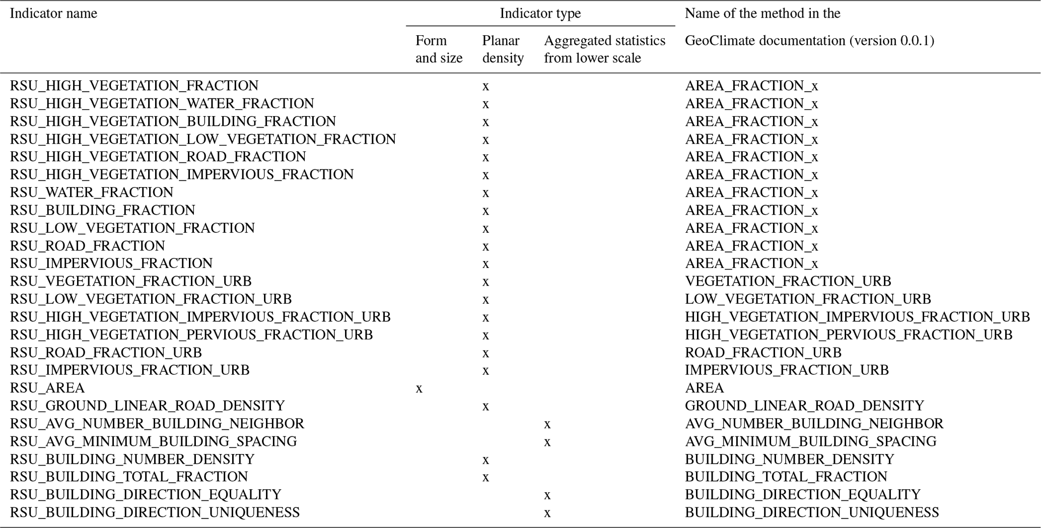
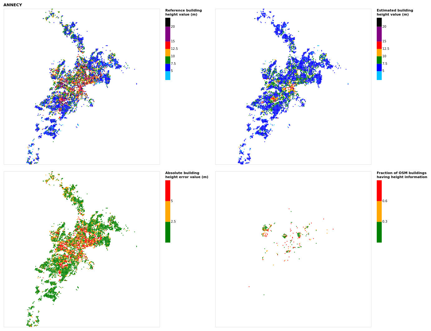
Figure B1Results for the commune at grid cell (upper left panel) reference building height, (upper right panel) estimated building height, (lower left panel) absolute building height error, and (lower right panel) fraction of OSM buildings that have height information. For all panels except the lower right, only cells that have buildings – with at least 90 % of their buildings having no height value in OSM – are displayed.
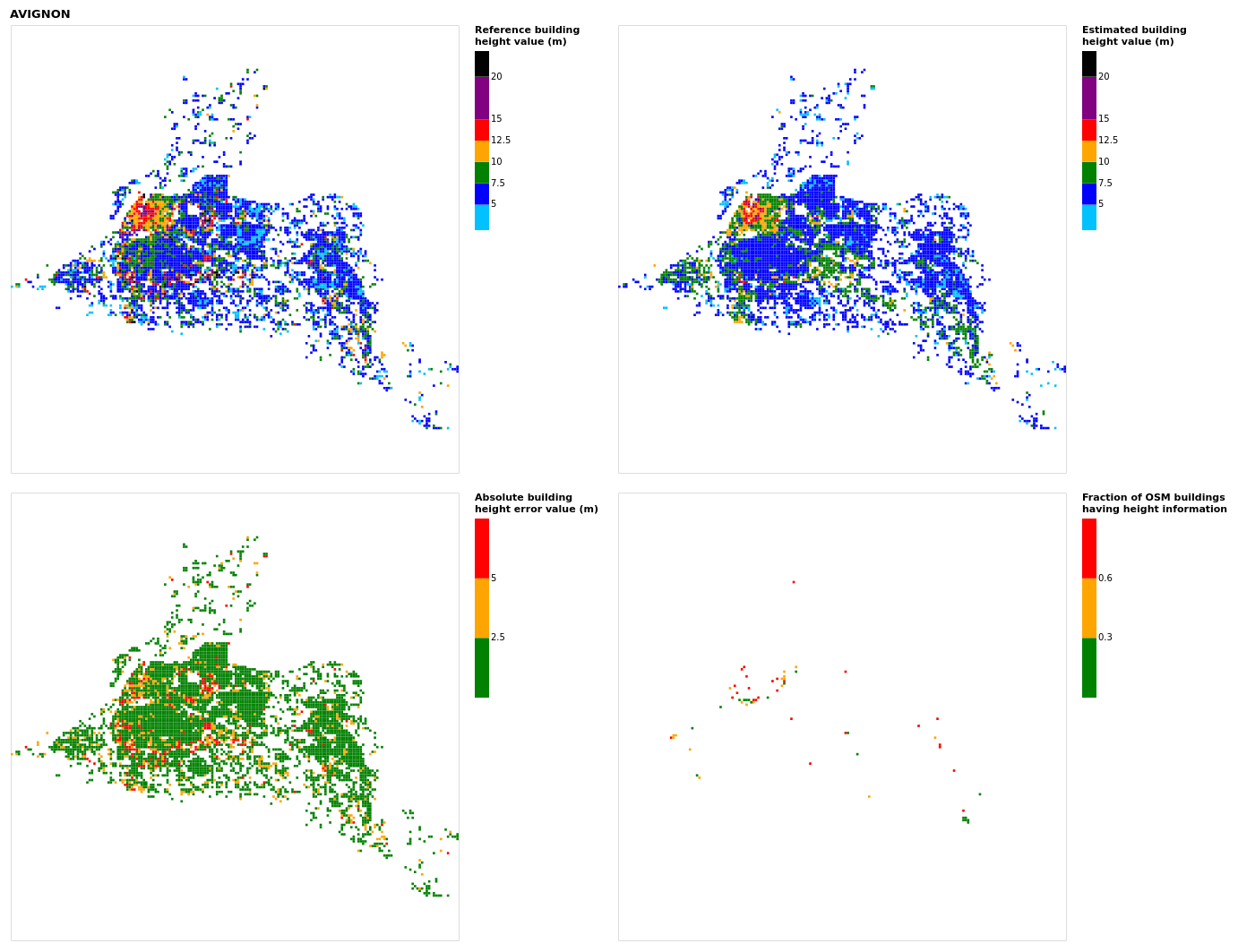
Figure B2Results for the commune at grid cell (upper left panel) reference building height, (upper right panel) estimated building height, (lower left panel) absolute building height error, and (lower right panel) fraction of OSM buildings having height information. For all panels except the lower right, only cells that buildings – with at least 90 % of their buildings having no height value in OSM – are displayed.
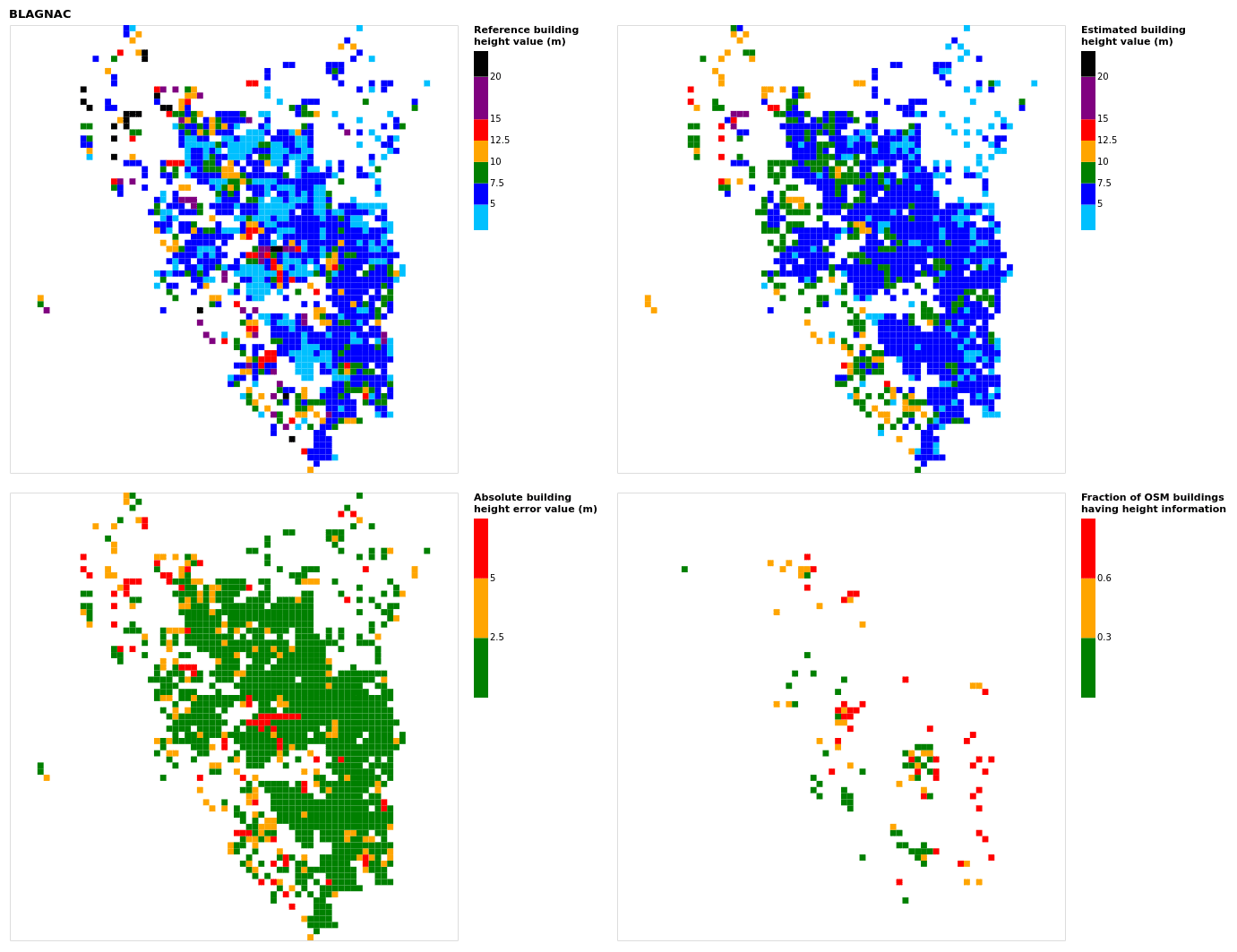
Figure B3Results for the commune at grid cell (upper left panel) reference building height, (upper right panel) estimated building height, (lower left panel) absolute building height error, and (lower right panel) fraction of OSM buildings that have height information. For all panels except the lower right, only cells that have buildings – with at least 90 % of their buildings having no height value in OSM – are displayed.
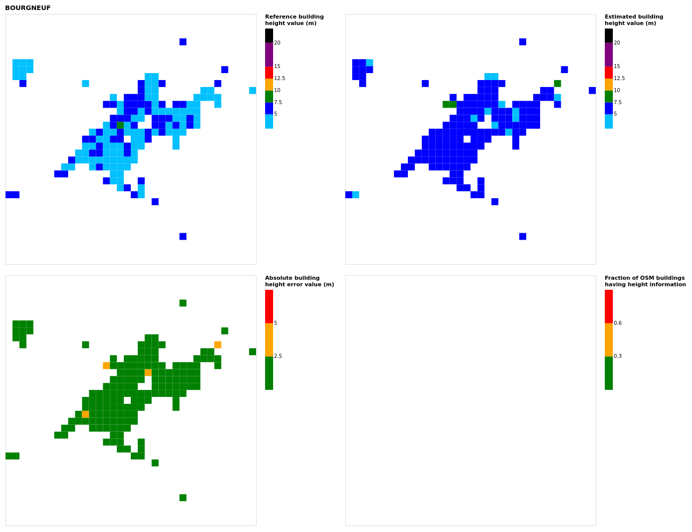
Figure B4Results for the commune at grid cell (upper left panel) reference building height, (upper right panel) estimated building height, (lower left panel) absolute building height error, and (lower right panel) fraction of OSM buildings that have height information. For all panels except the lower right, only cells that have buildings – with at least 90 % of their buildings having no height value in OSM – are displayed.
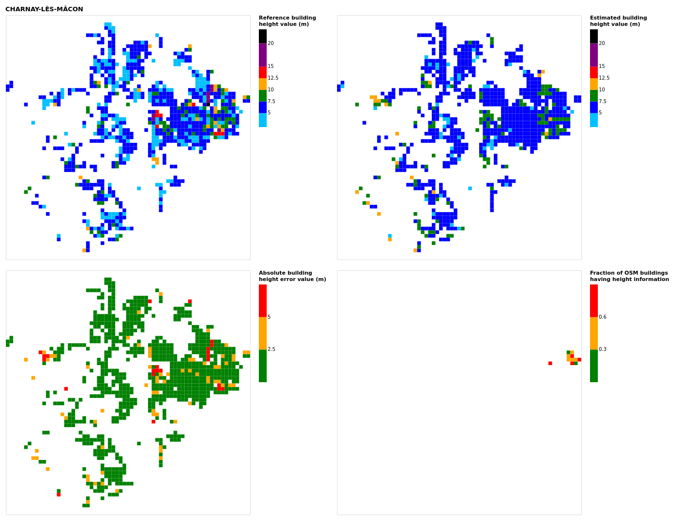
Figure B5Results for the commune at grid cell (upper left panel) reference building height, (upper right panel) estimated building height, (lower left panel) absolute building height error, and (lower right panel) fraction of OSM buildings that have height information. For all panels except the lower right, only cells that have buildings – with at least 90 % of their buildings having no height value in OSM – are displayed.
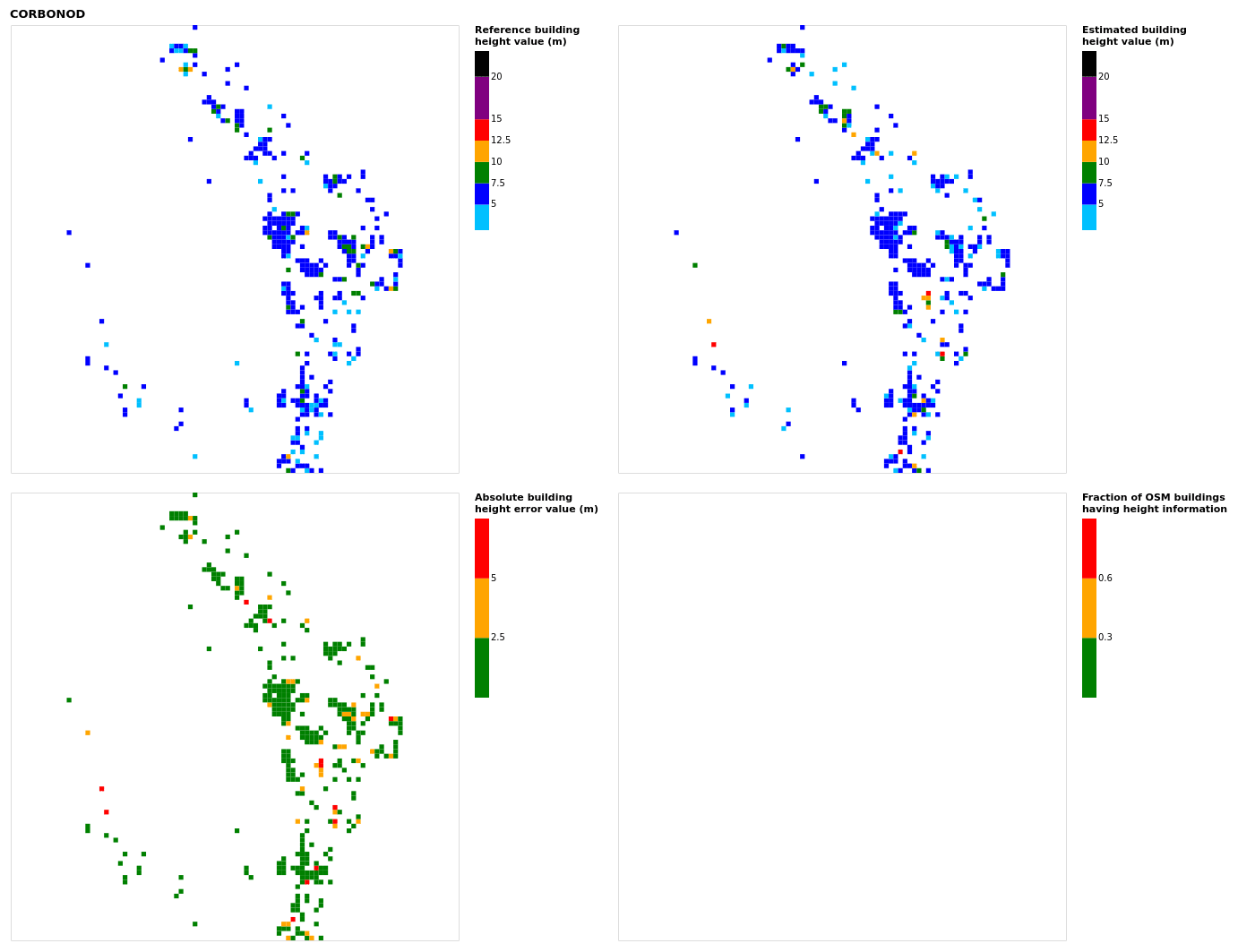
Figure B6Results for the commune at grid cell (upper left panel) reference building height, (upper right panel) estimated building height, (lower left panel) absolute building height error, and (lower right panel) fraction of OSM buildings that have height information. For all panels except the lower right, only cells that have buildings – with at least 90 % of their buildings having no height value in OSM – are displayed.
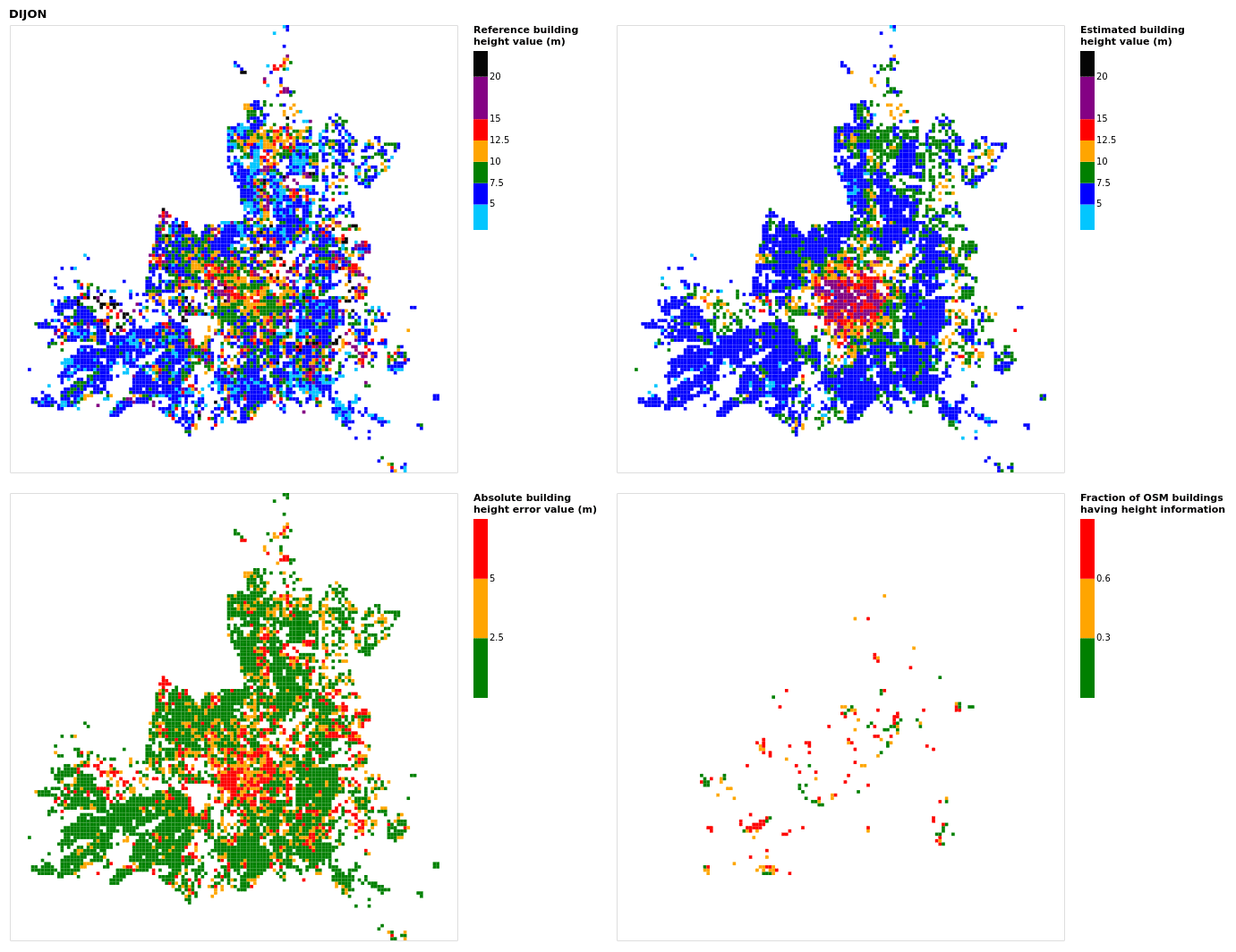
Figure B7Results for the commune at grid cell (upper left panel) reference building height, (upper right panel) estimated building height, (lower left panel) absolute building height error, and (lower right panel) fraction of OSM buildings that have height information. For all panels except the lower right, only cells that have buildings – with at least 90 % of their buildings having no height value in OSM – are displayed.
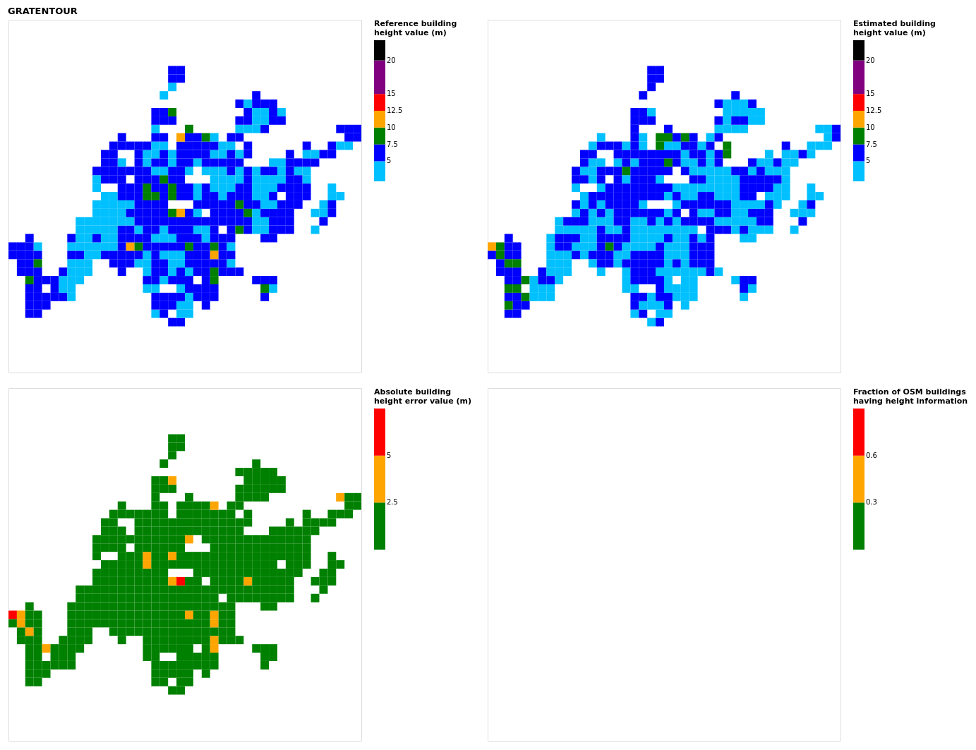
Figure B8Results for the commune at grid cell (upper left panel) reference building height, (upper right panel) estimated building height, (lower left panel) absolute building height error, and (lower right panel) fraction of OSM buildings that have height information. For all panels except the lower right, only cells that have buildings – with at least 90 % of their buildings having no height value in OSM – are displayed.
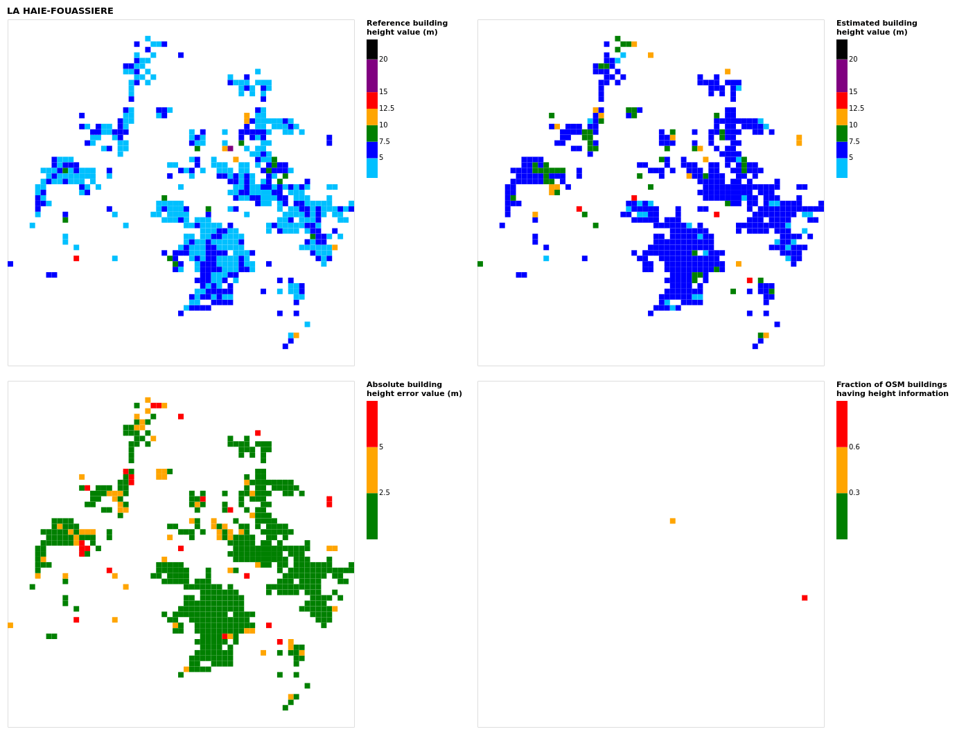
Figure B9Results for the commune at grid cell (upper left panel) reference building height, (upper right panel) estimated building height, (lower left panel) absolute building height error, and (lower right panel) fraction of OSM buildings that have height information. For all panels except the lower right, only cells that have buildings – with at least 90 % of their buildings having no height value in OSM – are displayed.
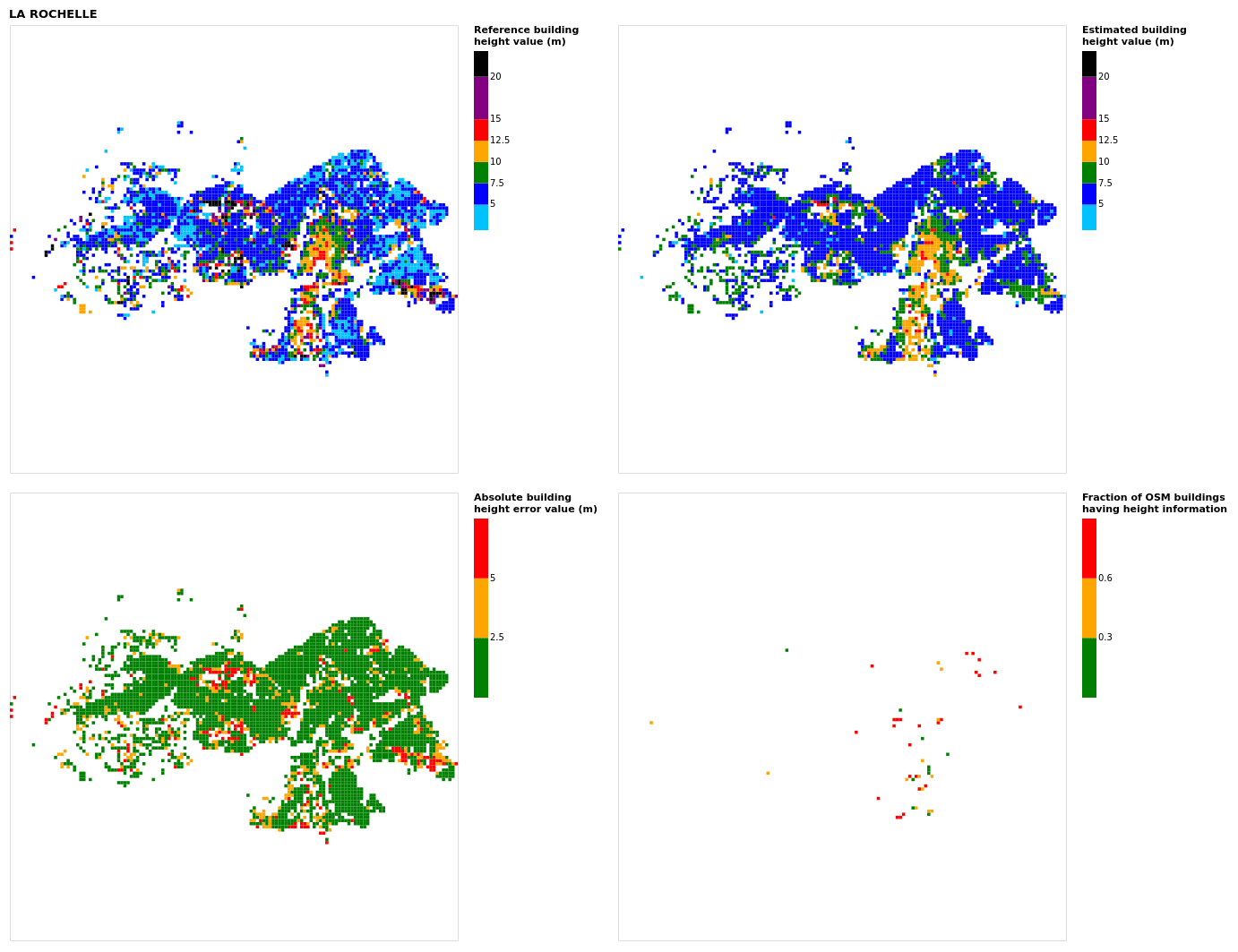
Figure B10Results for the commune at grid cell (upper left panel) reference building height, (upper right panel) estimated building height, (lower left panel) absolute building height error, and (lower right panel) fraction of OSM buildings that have height information. For all panels except the lower right, only cells that have buildings – with at least 90 % of their buildings having no height value in OSM – are displayed.
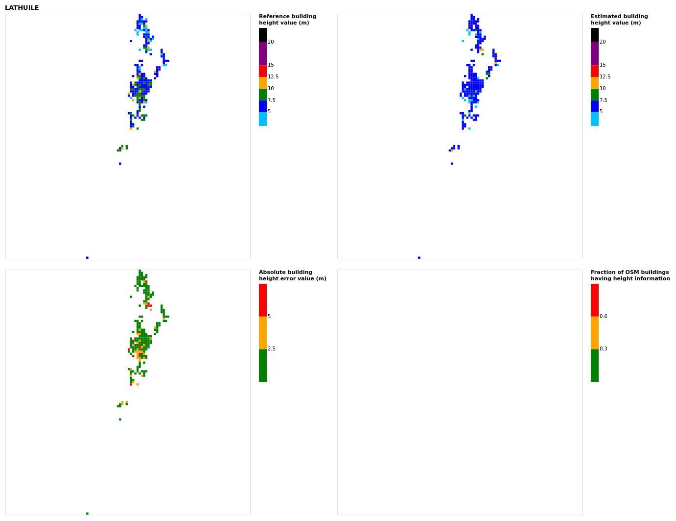
Figure B11Results for the commune at grid cell (upper left panel) reference building height, (upper right panel) estimated building height, (lower left panel) absolute building height error, and (lower right panel) fraction of OSM buildings that have height information. For all panels except the lower right, only cells that have buildings – with at least 90 % of their buildings having no height value in OSM – are displayed.
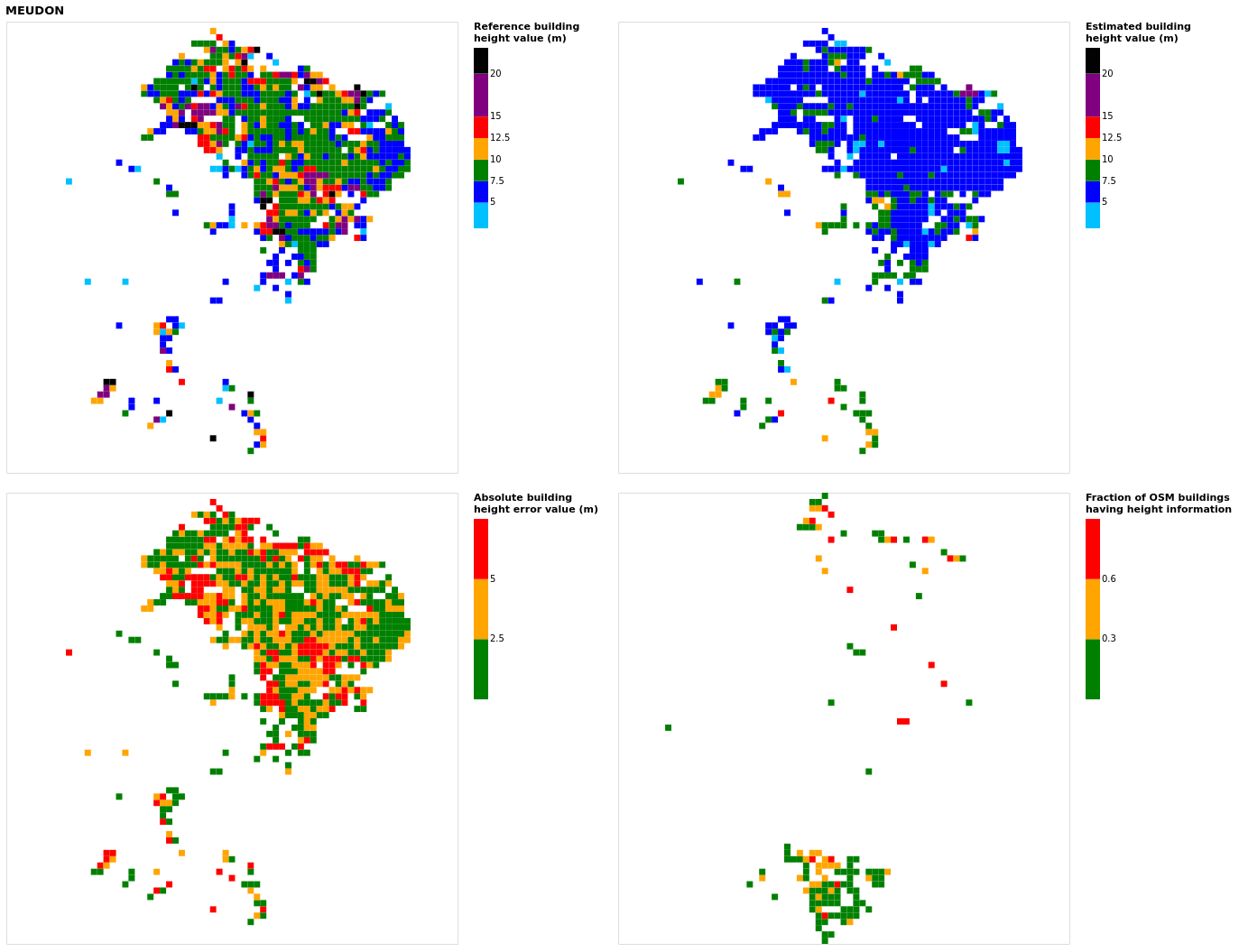
Figure B12Results for the commune at grid cell (upper left panel) reference building height, (upper right panel) estimated building height, (lower left panel) absolute building height error, and (lower right panel) fraction of OSM buildings that have height information. For all panels except the lower right, only cells that have buildings – with at least 90 % of their buildings having no height value in OSM – are displayed.
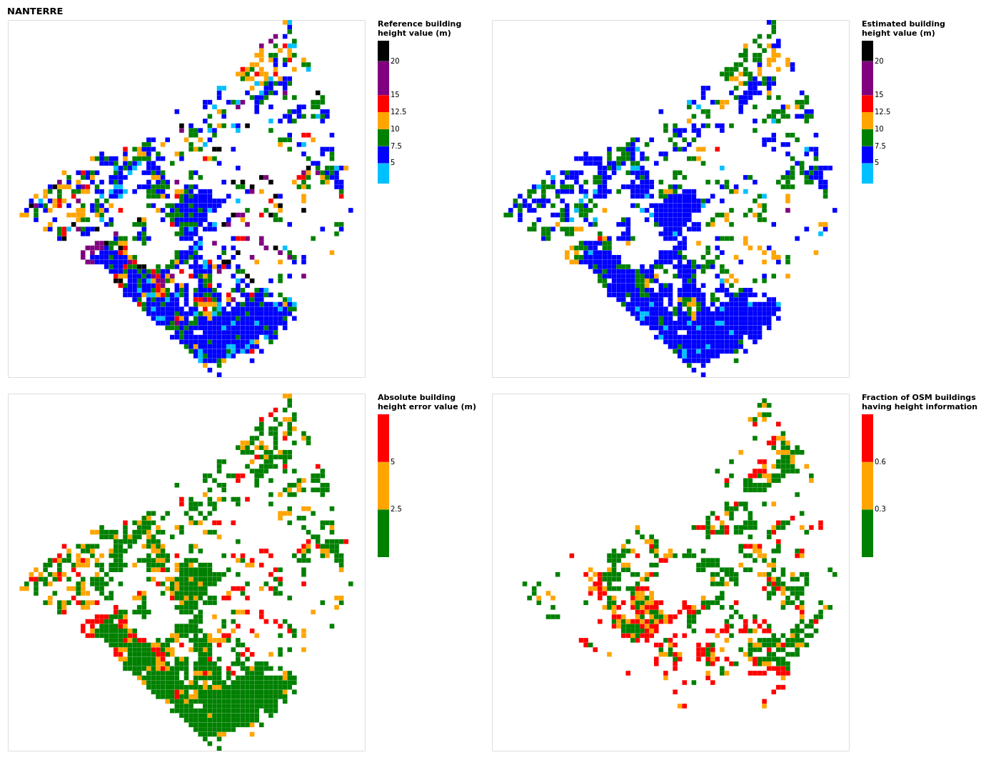
Figure B13Results for the commune at grid cell (upper left panel) reference building height, (upper right panel) estimated building height, (lower left panel) absolute building height error, and (lower right panel) fraction of OSM buildings that have height information. For all panels except the lower right, only cells that have buildings – with at least 90 % of their buildings having no height value in OSM – are displayed.
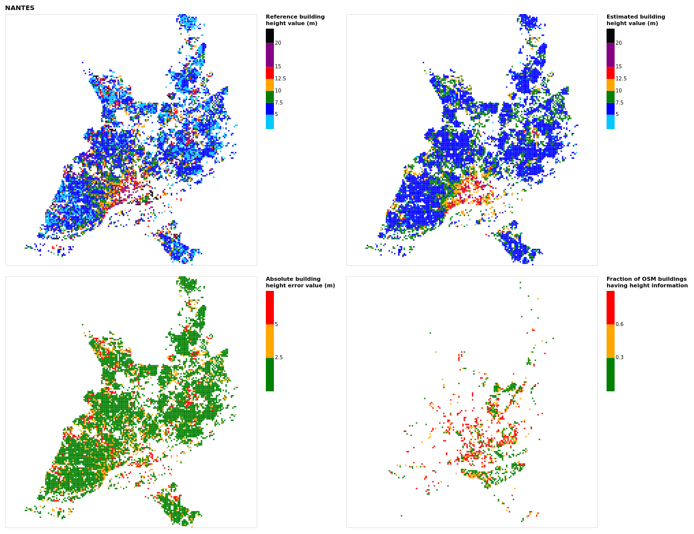
Figure B14Results for the commune at grid cell (upper left panel) reference building height, (upper right panel) estimated building height, (lower left panel) absolute building height error and (lower right panel) fraction of OSM buildings that have height information. For all panels except the lower right, only cells that have buildings – with at least 90 % of their buildings having no height value in OSM – are displayed.
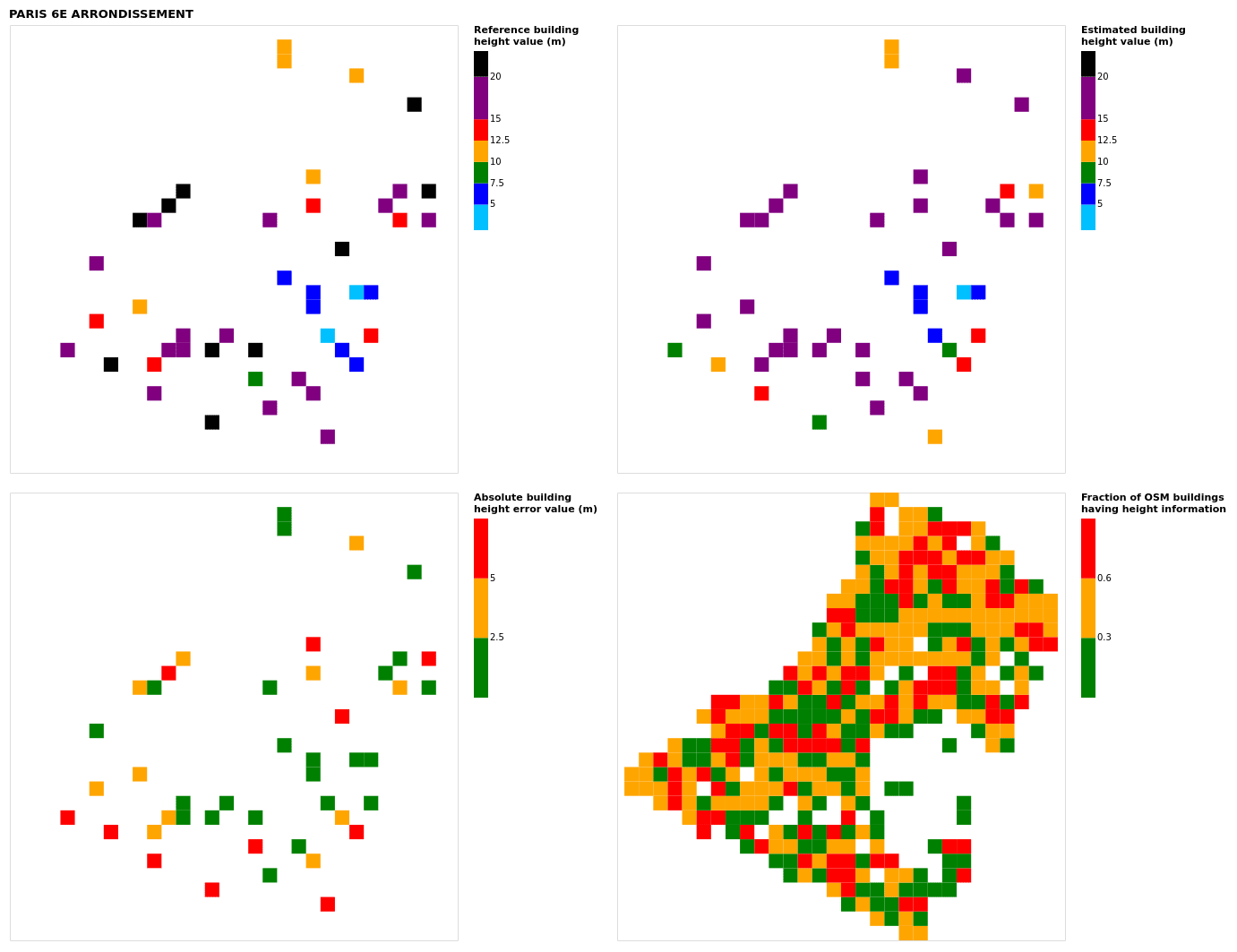
Figure B15Results for the commune at grid cell (upper left panel) reference building height, (upper right panel) estimated building height, (lower left panel) absolute building height error, and (lower right panel) fraction of OSM buildings that have height information. For all panels except the lower right, only cells that have buildings – with at least 90 % of their buildings having no height value in OSM – are displayed.
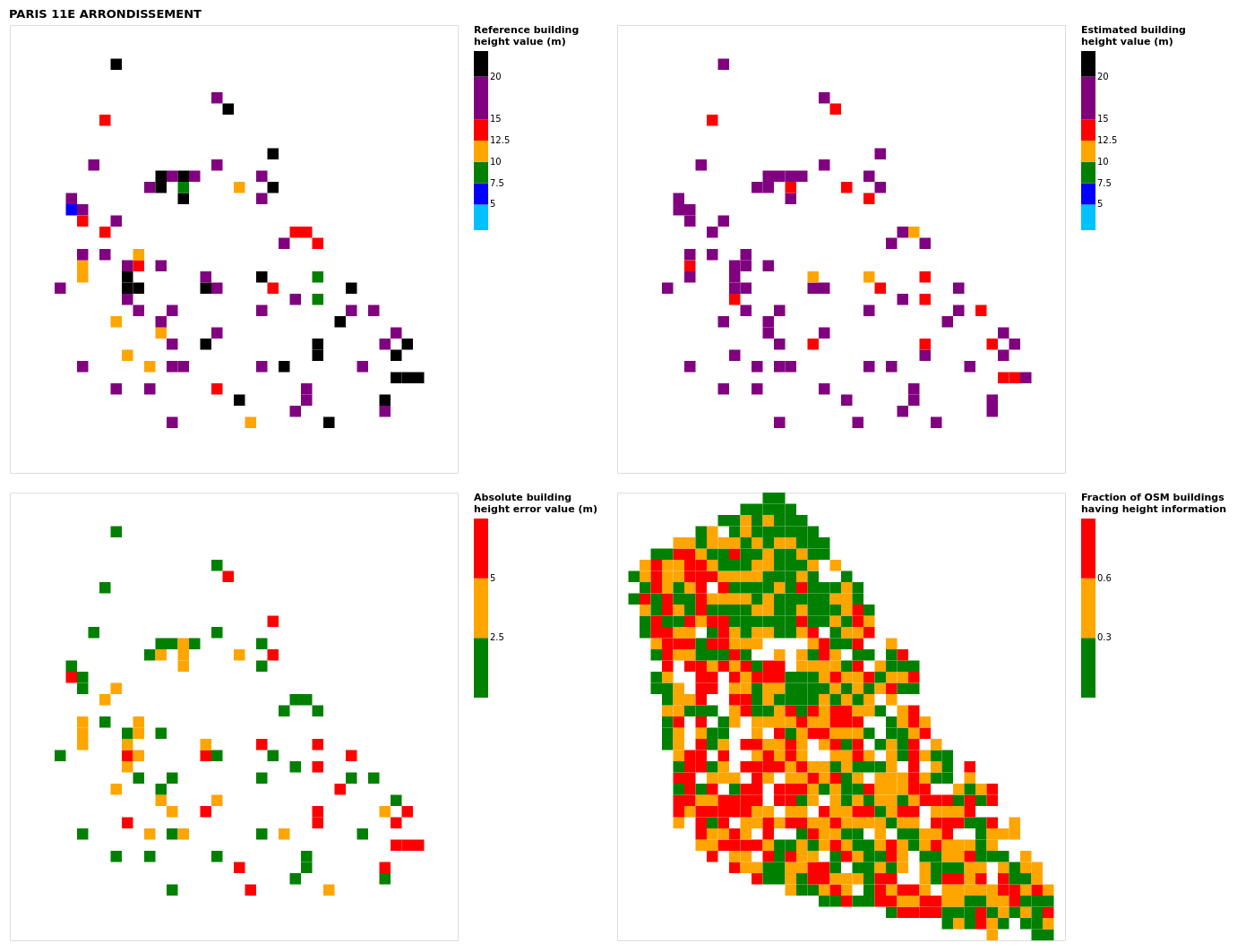
Figure B16Results for the commune at grid cell (upper left panel) reference building height, (upper right panel) estimated building height, (lower left panel) absolute building height error, and (lower right panel) fraction of OSM buildings that have height information. For all panels except the lower right, only cells that have buildings – with at least 90 % of their buildings having no height value in OSM – are displayed.

Figure B17Results for the commune at grid cell (upper left panel) reference building height, (upper right panel) estimated building height, (lower left panel) absolute building height error, and (lower right panel) fraction of OSM buildings that have height information. For all panels except the lower right, only cells that have buildings – with at least 90 % of their buildings having no height value in OSM – are displayed.

Figure B18Results for the commune at grid cell (upper left panel) reference building height, (upper right panel) estimated building height, (lower left panel) absolute building height error, and (lower right panel) fraction of OSM buildings that have height information. For all panels except the lower right, only cells that have buildings – with at least 90 % of their buildings having no height value in OSM – are displayed.
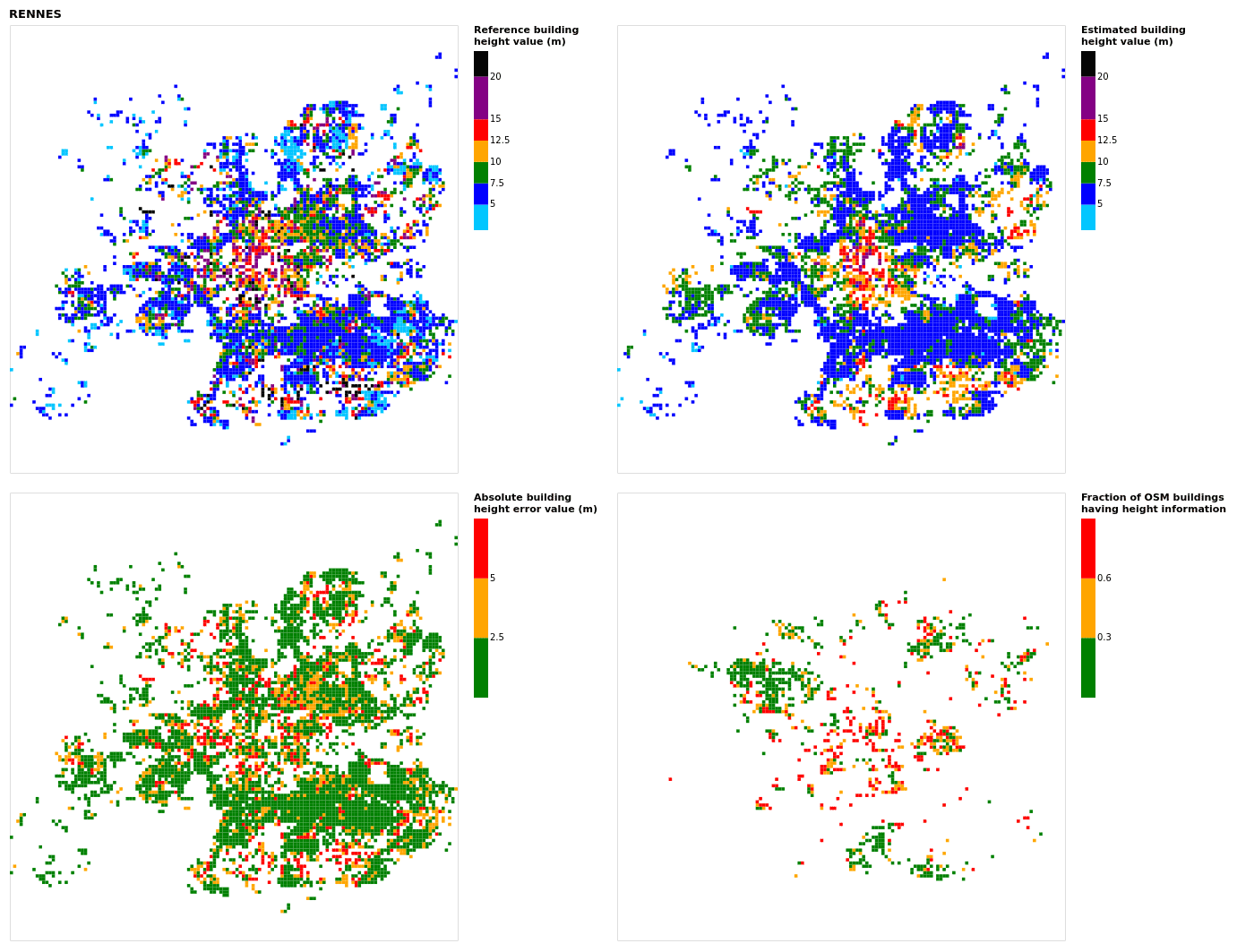
Figure B19Results for the commune at grid cell (upper left panel) reference building height, (upper right panel) estimated building height, (lower left panel) absolute building height error, and (lower right panel) fraction of OSM buildings that have height information. For all panels except the lower right, only cells that have buildings – with at least 90 % of their buildings having no height value in OSM – are displayed.
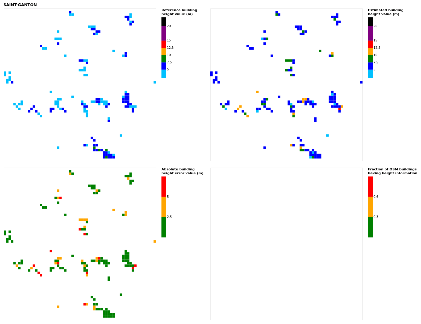
Figure B20Results for the commune at grid cell (upper left panel) reference building height, (upper right panel) estimated building height, (lower left panel) absolute building height error, and (lower right panel) fraction of OSM buildings that have height information. For all panels except the lower right, only cells that have buildings – with at least 90 % of their buildings having no height value in OSM – are displayed.
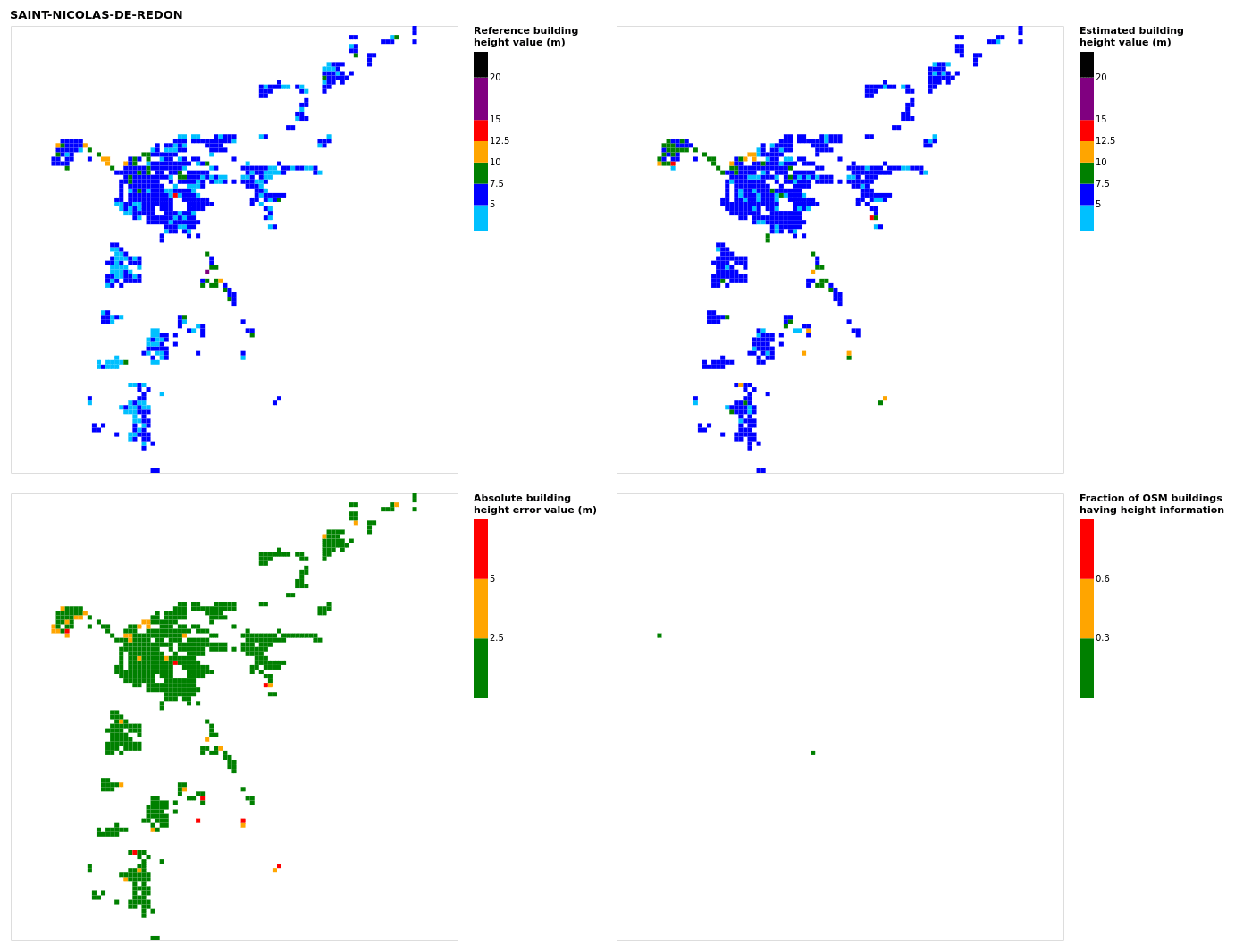
Figure B21Results for the commune at grid cell (upper left panel) reference building height, (upper right panel) estimated building height, (lower left panel) absolute building height error, and (lower right panel) fraction of OSM buildings that have height information. For all panels except the lower right, only cells that have buildings – with at least 90 % of their buildings having no height value in OSM – are displayed.
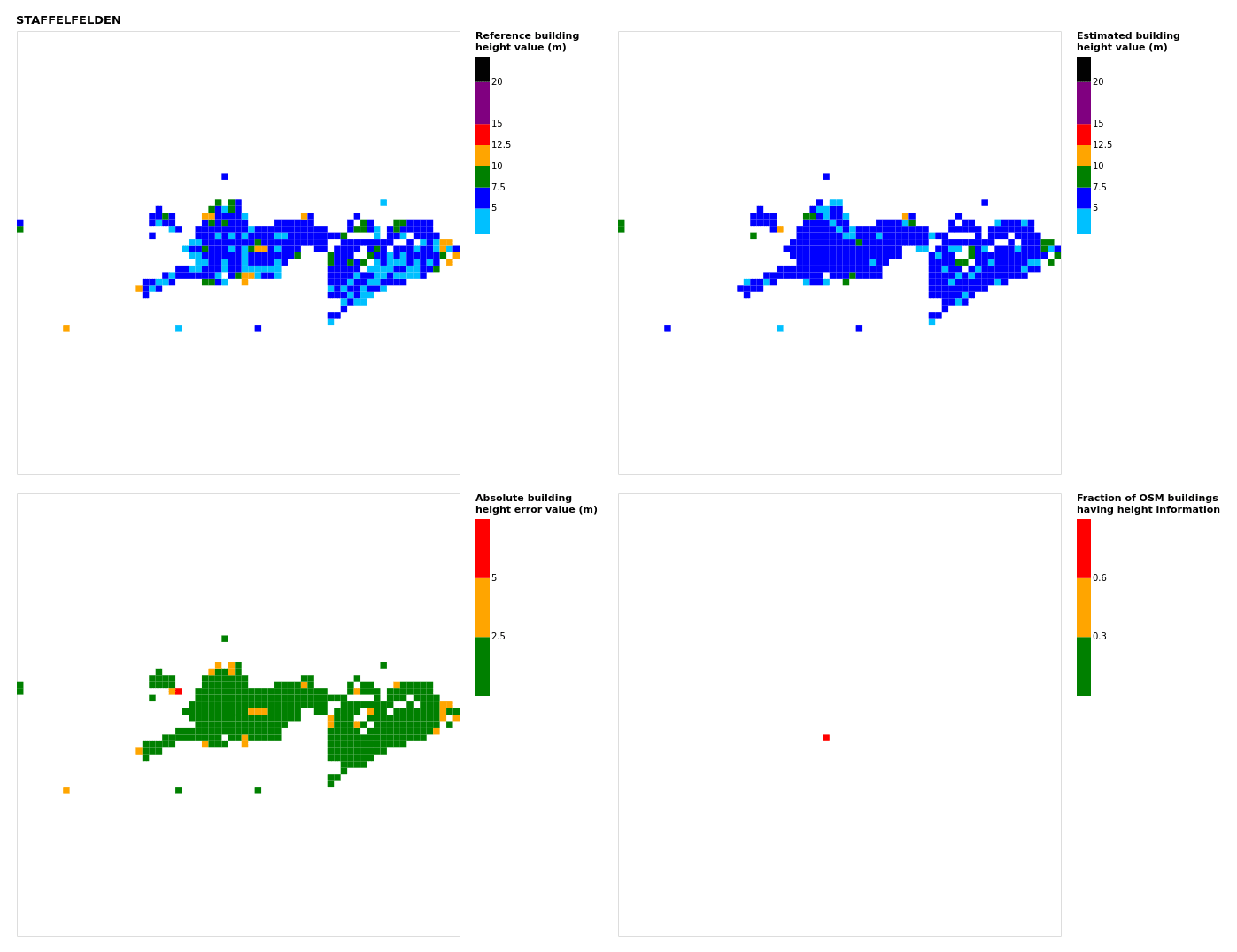
Figure B22Results for the commune at grid cell (upper left panel) reference building height, (upper right panel) estimated building height, (lower left panel) absolute building height error, and (lower right panel) fraction of OSM buildings that have height information. For all panels except the lower right, only cells that have buildings – with at least 90 % of their buildings having no height value in OSM – are displayed.
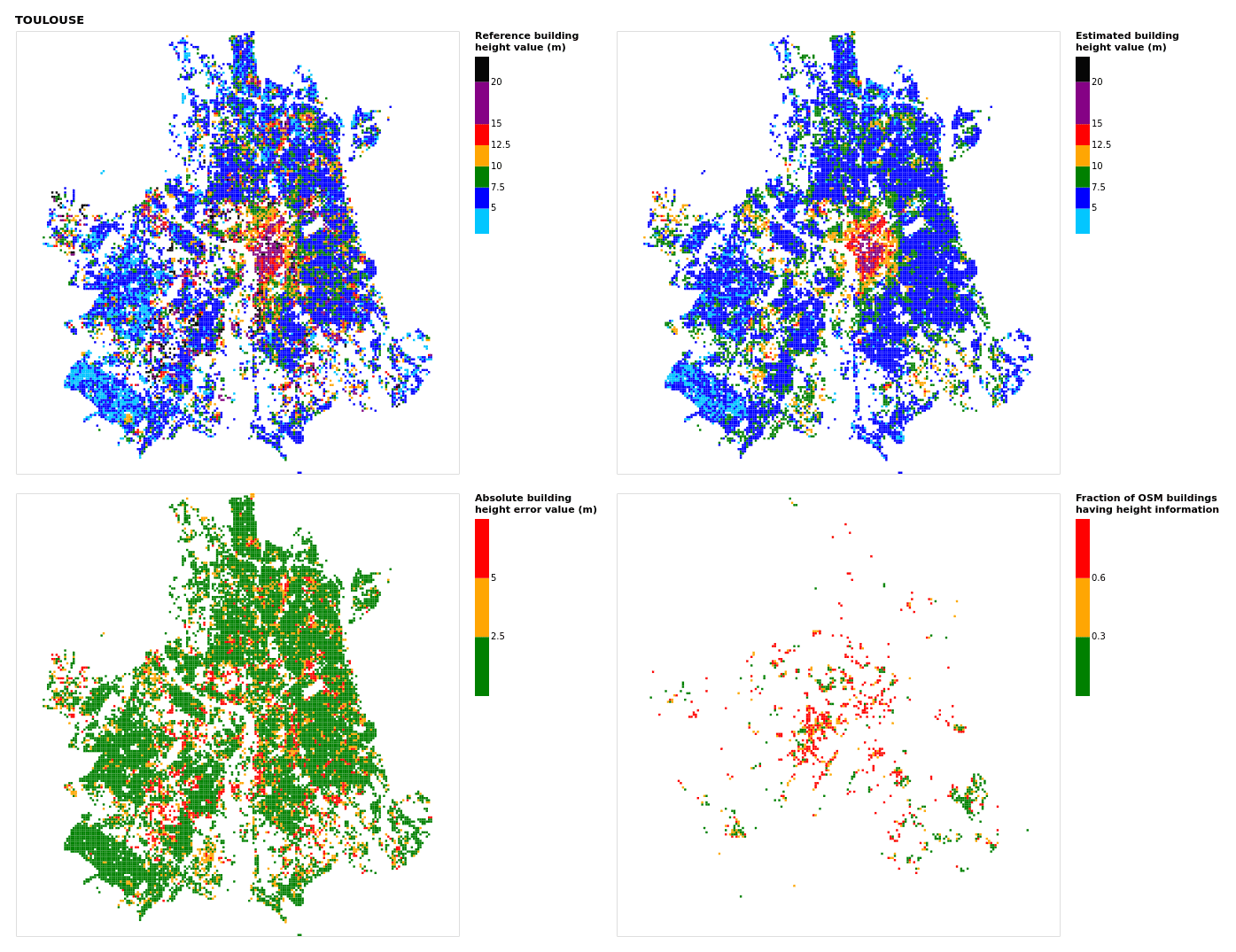
Figure B23Results for the commune at grid cell (upper left panel) reference building height, (upper right panel) estimated building height, (lower left panel) absolute building height error, and (lower right panel) fraction of OSM buildings that have height information. For all panels except the lower right, only cells that have buildings – with at least 90 % of their buildings having no height value in OSM – are displayed.
The major part of this work can be reproduced directly using the Software GeoClimate version 0.0.1 (the source code and executable file of this software version are permanently available on Zenodo at https://doi.org/10.5281/zenodo.6372337, Bocher et al., 2021b); the scripts and data are available on Zenodo at https://doi.org/10.5281/zenodo.6855063 (Bernard et al., 2021). GeoClimate downloads OpenStreetMap data using the overpass API from the end point https://overpass-api.de/ (last access: 28 September 2022), estimates building height when missing and calculates geographical indicators. The resulting datasets presented in this paper have been obtained using the OpenStreetMap data between June and September 2021. It can be freely accessed at https://doi.org/10.5281/zenodo.6855063 (Bernard et al., 2021). The French BDTopo (version 2.2) is used only for training and evaluation purposes. It is a proprietary dataset provided by the French National Geographic Institute (IGN) and is available upon request. Thus it is unfortunately not possible to make this dataset freely accessible. This was one of the major motivations for perform this work, i.e., to create a methodology to automatically create a topographic dataset containing buildings with estimated height.
The conceptualization was performed by JB, EB and VM, the data curation by JB, EB and ELS, the formal analysis by JB, EB, ELS and FL, the acquisition of the funding by EB and ELS, the investigation, the definition of the methodology and the project administration by JB and EB, the resources by EB, the software development by EB, JB, ELS and FL, the supervision of all tasks by JB and EB, the validation of the work by EB, JB, ELS and FL, the work dedicated to visualization by JB and EB, the original draft preparation by JB and EB, the review and editing by JB, EB, FL, ELS and VM.
The contact author has declared that none of the authors has any competing interests.
Publisher's note: Copernicus Publications remains neutral with regard to jurisdictional claims in published maps and institutional affiliations.
The method presented in this paper has been integrated in the GeoClimate tool and developed within the following research projects:
-
URCLIM (2017–2021), part of ERA4CS, a project initiated by JPI Climate and co-funded by the European Union under grant agreement no. 690462
-
CENSE (2017–2021), funded by the French National Research Agency (ANR) under grant agreement no. Projet-ANR-16-CE22-0012
-
SLIM (2020–2021), a Copernicus project C3S_432 Provisions to Environmental Fore- casting Applications (Lot 2).
The article processing charges for this open-access publication were covered by the Gothenburg University Library.
This paper was edited by Richard Mills and reviewed by two anonymous referees.
Bernabé, A., Musy, M., Andrieu, H., and Calmet, I.: Radiative properties of the urban fabric derived from surface form analysis: A simplified solar balance model, Sol. Energy, 122, 156–168, 2015. a
Bernard, J., Bocher, E., Petit, G., and Palominos, S.: Sky View Factor Calculation in Urban Context: Computational Performance and Accuracy Analysis of Two Open and Free GIS Tools, Climate, 6, 60, https://doi.org/10.3390/cli6030060, 2018. a
Bernard, J., Bocher, E., Wiederhold, E. L. S., Leconte, F., Masson, V., and Noûs, C.: Estimated height of the OpenStreetMap buildings of 24 French communes using the GeoClimate Software (version 0.0.1), Zenodo, https://doi.org/10.5281/zenodo.6855063, 2021. a, b, c, d
Biljecki, F., Ledoux, H., and Stoter, J.: Generating 3D city models without elevation data, Computers, Environment and Urban Systems, 64, 1–18, 2017. a, b, c, d
Bocher E., Bernard J., Le Saux Wiederhold E., Leconte F., Petit G., Palominos S., and Noûs C.: GeoClimate: a Geospatial processing toolbox for environmental and climate studies, Zenodo, https://doi.org/10.5281/zenodo.5534680, 2021a. a, b
Bocher E., Bernard J., Le Saux Wiederhold E., Leconte F., Petit G., Palominos S., and Noûs C.: GeoClimate: a Geospatial processing toolbox for environmental and climate studies (0.0.1), Zenodo, https://doi.org/10.5281/zenodo.6372337, 2021b. a, b
Bocher, E., Guillaume, G., Picaut, J., Petit, G., and Fortin, N.: NoiseModelling: An Open Source GIS Based Tool to Produce Environmental Noise Maps, ISPRS Int. J. Geo-Inf., 8, 130, https://doi.org/10.3390/ijgi8030130, 2019. a
Bocher, E., Bernard, J., Wiederhold, E. L. S., Leconte, F., Petit, G., Palominos, S., and Noûs, C.: GeoClimate: a Geospatial processing toolbox for environmental and climate studies, Journal of Open Source Software, 6, 3541, https://doi.org/10.21105/joss.03541, 2021. a, b
Cao, Y. and Huang, X.: A deep learning method for building height estimation using high-resolution multi-view imagery over urban areas: A case study of 42 Chinese cities, Remote Sens. Environ., 264, 112590, https://doi.org/10.1016/j.rse.2021.112590, 2021. a
Fradkin, M., Roux, M., Maître, H., and Leloglu, U. M.: Surface reconstruction from multiple aerial images in dense urban areas, in: Proceedings. 1999 IEEE Computer Society Conference on Computer Vision and Pattern Recognition (Cat. No PR00149), 2, 262–267, IEEE, 1999. a
Hanna, S. R. and Britter, R. E.: Wind flow and vapor cloud dispersion at industrial and urban sites, vol. 7, John Wiley and Sons, https://doi.org/10.1002/9780470935613, 2010. a, b, c
Hastie, T., Tibshirani, R., and Friedman, J.: Data mining, inference, and prediction, The elements of statistical learning Springer Series in Statistics, Springer-Verlag, New York, https://doi.org/10.1007/978-0-387-84858-7, 2001. a, b
INSEE: Method for determining functional areas in 2020, 2020. a, b
Johansson, L., Onomura, S., Lindberg, F., and Seaquist, J.: Towards the modelling of pedestrian wind speed using high-resolution digital surface models and statistical methods, Theor. Appl. Climatol., 124, 189–203, 2016. a
Lao, J., Bocher, E., Petit, G., Palominos, S., Le Saux, E., and Masson, V.: Is OpenStreetMap suitable for urban climate studies?, in: OGRS2018, Open Source Geospatial Research and Education Symposium, 9–11 October 2018, Lugano, Switzerland, https://halshs.archives-ouvertes.fr/halshs-01898612 (last access: 19 Sptember 2022), 2018. a
Lindberg, F.: Modelling the urban climate using a local governmental geo-database, Meteorol. Appl., 14, 263–273, https://doi.org/10.1002/met.29, 2007. a
Masson, V., Heldens, W., Bocher, E., Bonhomme, M., Bucher, B., Burmeister, C., de Munck, C., Esch, T., Hidalgo, J., Kanani-Sühring, F., Kwok, Y.-T., Lemonsu, A., Lévy, J.-P., Maronga, B., Pavlik, D., Petit, G., See, L., Schoetter, R., Tornay, N., Votsis, A., and Zeidler, J.: City-descriptive input data for urban climate models: Model requirements, data sources and challenges, Urban Climate, 31, 100536, https://doi.org/10.1016/j.uclim.2019.100536, 2020. a
Milojevic-Dupont, N., Hans, N., Kaack, L. H., Zumwald, M., Andrieux, F., de Barros Soares, D., Lohrey, S., Pichler, P.-P., and Creutzig, F.: Learning from urban form to predict building heights, PLOS ONE, 15, e0242010, https://doi.org/10.1371/journal.pone.0242010, 2020. a, b
Mocnik, F.-B., Zipf, A., and Raifer, M.: The OpenStreetMap folksonomy and its evolution, Geo-spatial Information Science, 20, 219–230, 2017. a
Oke, T. R.: Boundary layer climates, 2nd ed., Routledge, https://doi.org/10.4324/9780203407219, 2002. a
Shan, J. and Toth, C. K.: Topographic laser ranging and scanning: principles and processing, 2nd ed., CRC press, https://doi.org/10.1201/9781315154381, 2018. a
Shao, Y., Taff, G. N., and Walsh, S. J.: Shadow detection and building-height estimation using IKONOS data, Int. J. Remote, 32, 6929–6944, 2011. a
Sohn, G., Huang, X., and Tao, V.: Using a binary space partitioning tree for reconstructing polyhedral building models from airborne lidar data, Photogramm. Eng. Rem. S., 74, 1425–1438, 2008. a
Song, H., Huang, B., and Zhang, K.: Shadow detection and reconstruction in high-resolution satellite images via morphological filtering and example-based learning, IEEE T. Geosci. Remote, 52, 2545–2554, 2013. a
Tang, U. and Wang, Z.: Influences of urban forms on traffic-induced noise and air pollution: Results from a modelling system, Environ. Modell. Softw., 22, 1750–1764, https://doi.org/10.1016/j.envsoft.2007.02.003, 2007. a
Zeng, C., Wang, J., Zhan, W., Shi, P., and Gambles, A.: An elevation difference model for building height extraction from stereo-image-derived DSMs, Int. J. Remote, 35, 7614–7630, 2014. a
https://www.openstreetmap.org (last access: 19 September 2022)
- Abstract
- Introduction
- Data and method
- Results and discussions
- Conclusions
- Appendix A: List of all spatial indicators used as independent variables
- Appendix B: Results for all cities
- Code and data availability
- Author contributions
- Competing interests
- Disclaimer
- Acknowledgements
- Financial support
- Review statement
- References