the Creative Commons Attribution 4.0 License.
the Creative Commons Attribution 4.0 License.
 | 10 Oct 2022
Tropospheric transport and unresolved convection: numerical experiments with CLaMS 2.0/MESSy
Mengchu Tao
Marc von Hobe
Lars Hoffmann
Corinna Kloss
Fabrizio Ravegnani
C. Michael Volk
Valentin Lauther
Andreas Zahn
Peter Hoor
Felix Ploeger
Pure Lagrangian, i.e., trajectory-based transport models, take into account only the resolved advective part of transport. That means neither mixing processes between the air parcels (APs) nor unresolved subgrid-scale advective processes like convection are included. The Chemical Lagrangian Model of the Stratosphere (CLaMS 1.0) extends this approach by including mixing between the Lagrangian APs parameterizing the small-scale isentropic mixing. To improve model representation of the upper troposphere and lower stratosphere (UTLS), this approach was extended by taking into account parameterization of tropospheric mixing and unresolved convection in the recently published CLaMS 2.0 version. All three transport modes, i.e., isentropic and tropospheric mixing and the unresolved convection can be adjusted and optimized within the model. Here, we investigate the sensitivity of the model representation of tracers in the UTLS with respect to these three modes.
For this reason, the CLaMS 2.0 version implemented within the Modular Earth Submodel System (MESSy), CLaMS 2.0/MESSy, is applied with meteorology based on the ERA-Interim (EI) and ERA5 (E5) reanalyses with the same horizontal resolution (1.0×1.0∘) but with 60 and 137 model levels for EI and E5, respectively. Comparisons with in situ observations are used to rate the degree of agreement between different model configurations and observations. Starting from pure advective runs as a reference and in agreement with CLaMS 1.0, we show that among the three processes considered, isentropic mixing dominates transport in the UTLS. Both the observed CO, O3, N2O, and CO2 profiles and CO–O3 correlations are clearly better reproduced in the model with isentropic mixing. The second most important transport process considered is convection which is only partially resolved in the vertical velocity fields provided by the analysis. This additional pathway of transport from the planetary boundary layer (PBL) to the main convective outflow dominates the composition of air in the lower stratosphere relative to the contribution of the resolved transport. This transport happens mainly in the tropics and sub-tropics, and significantly rejuvenates the age of air in this region. By taking into account tropospheric mixing, weakest changes in tracer distributions without any clear improvements were found.
- Article
(5891 KB) - Full-text XML
- BibTeX
- EndNote


Timescales of transport from the Earth's surface into the upper troposphere and lower stratosphere (UTLS) determine chemical composition of this region and, consequently, influence the Earth’s radiation budget and surface temperatures (Riese et al., 2012). The Lagrangian, i.e., trajectory-based, view of transport has proven to successfully trace back the origin of air during its long-range transport mainly because spatially and temporally highly resolved clouds of Lagrangian air parcels (APs) can by easily applied to study the selected parts of the flow (e.g., reverse domain filling technique, see Lin et al. (2013) and references therein). Due to a reduced numerical diffusion, small-scale structures of tracers are in general better reproduced by Lagrangian than Eulerian transport schemes although the gap between these two approaches became smaller over the last 2 decades (e.g., Lauritzen et al., 2014 and references therein).
However, Lagrangian models, which are driven by resolved advective winds (as provided e.g., by meteorological reanalyses) still miss important physical drivers of transport like unresolved (subgrid-scale) convection and all mixing processes including isentropic or other small-scale mainly tropospheric mixing processes. While parameterization of unresolved convection can be understood as an extension of the advective part of transport (additional updrafts and downdrafts), including of mixing requires an extra mass transfer between the APs, the latter being always a challenge in the irregular grid of Lagrangian APs. In general, motion in the free atmosphere can be divided into two parts: the 2D isentropic transport on surfaces with constant, dry, or moist potential temperature, and the cross-isentropic transport, roughly perpendicular to such surfaces. Sufficiently far away from the planetary boundary layer (PBL) and from regions affected by strong convection, the cross-isentropic transport, mainly driven by radiation, is much slower compared to fast isentropic transport typically disturbed by all types of waves and finally leading to irreversible, isentropic mixing. In addition, both PBL and convection are drivers of tropospheric mixing and have to be appropriately parameterized not only in the Lagrangian transport models.
Currently, there are only few Lagrangian transport models that include a parametrization of unresolved convection and mixing (Brinkop and Jöckel, 2019; Wohltmann et al., 2019; Konopka et al., 2019). Here we use the recently published CLaMS 2.0 version (Konopka et al., 2019), which extends the concept of isentropic mixing (CLaMS 1.0) by including tropospheric mixing and a simple parameterization of convective uplifts. In this paper, we aim to quantify the relative importance of these three unresolved transport modes using as a reference pure trajectory-based studies. Extending the approach presented in Konopka et al. (2019) and Wohltmann et al. (2019), we do it on a global scale and over time periods of more than 10 yr in order to find the impact of these new, rather tropospheric transport modes, even on the stratospheric composition. For validation, idealized tracers and comparisons with in situ observations of CO, O3, N2O, and CO2 are investigated. By studying ERA-Interim- and ERA5-driven CLaMS 2.0 transport, we also aim to enhance the overall agreement of the model with the observations, extending in this way results where Lagrangian transport within a climate model framework were investigated (Brinkop and Jöckel, 2019). Our main focus is to quantify the role of unresolved convective updrafts and of tropospheric mixing on the representation of climate-relevant trace gases in the UTLS region.
The setup of CLaMS 2.0/MESSy follows the CLaMS 2.0 configuration described in Konopka et al. (2019), and uses the Modular Earth Submodel System (MESSy) as a software framework (Jöckel et al., 2010) to run the model on the supercomputer JUWELS (Jülich Supercomputing Centre, 2019). To simplify the notation, we omit the suffix MESSy in the following. ERA-Interim (EI) and ERA5 (E5) reanalyses from the European Centre for Medium-Range Weather Forecasts (ECMWF) provide the meteorology to drive the model (Dee et al., 2011; Hersbach et al., 2020). Although the same horizontal resolution (1.0×1.0∘) is used for both data sets, the vertical resolution is different, with 60 and 137 levels for EI and E5, respectively, corresponding to the maximal vertical resolution available for these products. The vertical layer depths at 5 to 20 km altitude vary between 0.3 to 0.4 km for E5 and 0.5 to 1.4 km for EI. Hoffmann et al. (2019) found that transition from EI to E5 improves the Lagrangian transport simulations mainly due to improved representation of convective updrafts.
The baseline for the following comparisons is a CLaMS 1.0 set-up described by Pommrich et al. (2014), which covers the period 1979–2017 and is available in two versions driven by EI and E5, respectively. All CLaMS 2.0 simulations start on 1 January 2017, use CLaMS 1.0 for initialization, and cover 1 yr. We choose 2017 because data of two major aircraft campaigns covering tropics and extra-tropics are available (StratoClim and WISE, see Sect. 3.2), and the reanalyses products EI and E5 can be downloaded from the ECMWF server (EI only until mid of 2019). To check the long-term effects on tracer distributions for different model configurations described below, perpetuum runs are performed (14-times 2017) as described in Konopka et al. (2017) and Poshyvailo et al. (2018). Perpetuum runs approximate transient runs, which are numerically more expensive. Although such runs do not reproduce interannual variability and have a discontinuity by moving from 31 December to 1 January of the following year, they provide a cost-effective way to study model sensitivities related to different transport parameterizations and configurations. A short description of the differences between CLaMS 1.0, CLaMS 2.0, and the slightly modified CLaMS 2.0 version used here can be found in Table 1.
(Pommrich et al., 2014)(Konopka et al., 2019)Table 1Changes between CLaMS 1.0 (first column), CLaMS 2.0 (second column), and CLaMS 2.0 version used in this paper (third column, for details see Appendix).

Notation: Δζ (in K): thickness of the lowest model layer approximating the planetary boundary layer (PBL), values of Δζ=100 and 140 K correspond to a maximal geometric thickness of 2 and 3 km, respectively, of this orography following layer. r (in km): horizontal mean distance between the APs in the lowest model layer, λ (in d−1): (critical) Lyapunov exponent, ϵ: merging parameter, , (in s−2): (critical) dry and moist Brunt–Vaisala frequency, Δθc (in K) (critical) vertical uplift of convective updrafts, θ,ζ: potential and hybrid potential temperature (Mahowald et al., 2002). In CLaMS 2.0 version used here, the parameters of isentropic mixing approximate the intensity of isentropic mixing used in CLaMS 1.0. Furthermore, the horizontal resolution in the lowest layer was slightly enhanced (from 110 to 90 km) to fit better the input reanalysis.
Details of these modifications are explained in the Appendix. By simple redefining of the parameters listed in Table 1, CLaMS 2.0 can be run as CLaMS 1.0.
Thus, in CLaMS 2.0, there is an interplay between three parameterized components of transport: isentropic mixing (I), unresolved convection (C), and tropospheric mixing (T) schematically shown in Fig. 1.
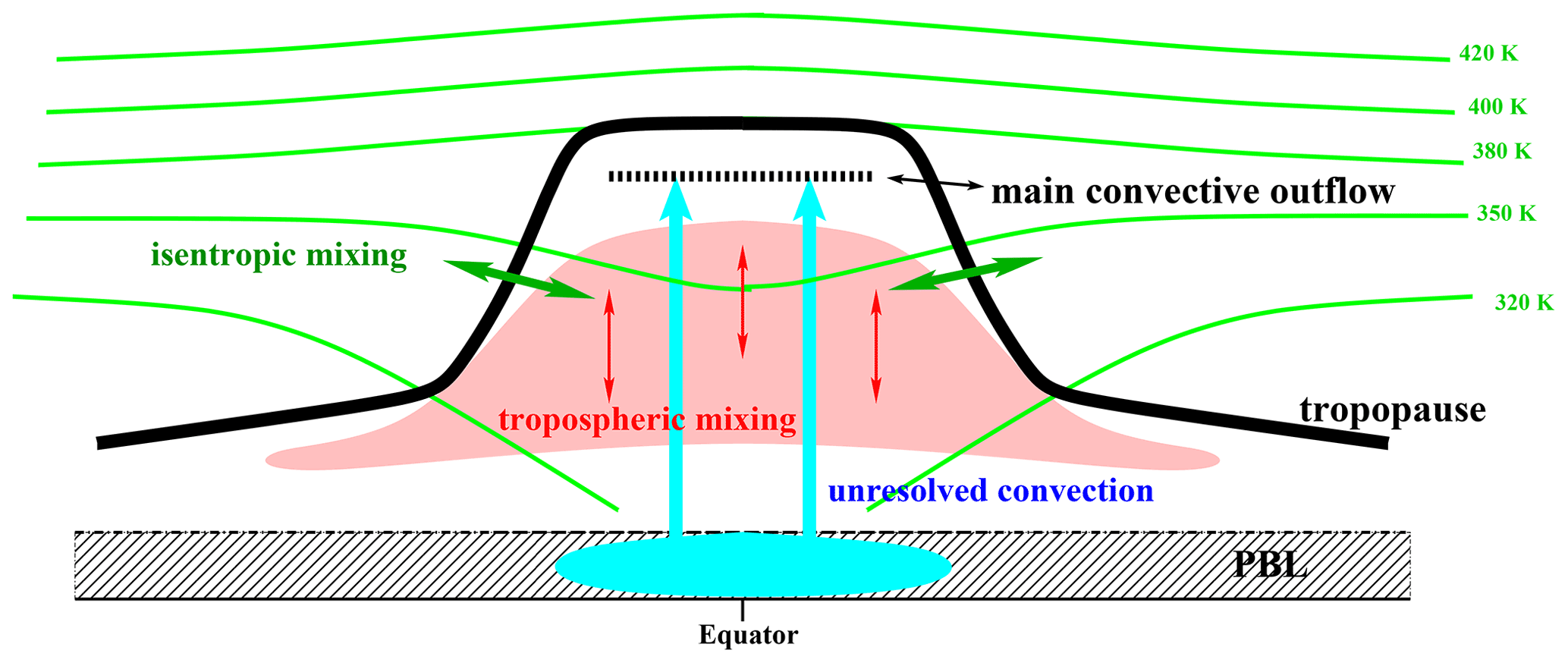
Figure 1In CLaMS 2.0, an interplay between three types of extended transport is investigated: isentropic mixing (CLaMS 1.0), tropospheric mixing, and unresolved convective updrafts (CLaMS 2.0). Extended transport means an extension relative to a pure trajectory-based transport that is used in this study as a reference.
In the following, configurations with respective components switched off and on are denoted with “0” and “1”, respectively. Because we do not carry out any systematic sensitivity of their strength, the choice “1” means a configuration with rather too strong contribution of the respective component. All performed runs are listed in Table 2.
Table 2List of performed runs. As a baseline, CLaMS 1.0 runs are used. For pure advection runs (I0C0T0), 54 instead of 45 layers were used to get similar number of air parcels like in the runs with all transport modes switched on (I1C1T1). Suffix EI (ERA-Interim) or E5 (ERA5) is used in the text and figures to denote the respective reanalysis driving CLaMS. All runs are performed within the software framework MESSy and are also available as perpetuum runs (14-times 2017).

If all transport extensions are switched on (i.e., for I1, C1, T1), the following values of the model parameters introduced in Table 1 are used:
Thus, isentropic mixing (I) is controlled by the Lyapunov exponent λ and the mixing frequency Δt defining the critical deformations in the flow, λΔt, and the merging parameter ϵ controlling the intensity of the grid adaption procedure including new air APs into the flow (see Appendix for more details). The different choice of mixing parameters compared to CLaMS 1.0 is owed to the fact that in order resolve the diurnal cycle of convective updrafts, higher mixing frequency, without any significant change of the total intensity of mixing, is required (every 6 h in CLaMS 2.0 instead of every 24 h in CLaMS 1.0). Thus, the convection parametrization (C) is called 4 times per day; the crudest possible approximation of the diurnal cycle of convection. Intensity of convection is regulated by the moist Brunt–Vaisala frequency triggering its onset in the PBL and by the minimal vertical uplift Δθc deciding which convective updrafts are taken into account. Finally, the dry Brunt–Vaisala frequency controls the onset of tropospheric mixing, i.e., APs with smaller than a critical value are mixed by averaging the mixing ratios of a considered AP with all its next neighbors. A stably stratified stratosphere, with typical values of the Brunt–Vaisala frequency much larger than , prevents this type of mixing. We coined this type of mixing “tropospheric mixing” because it happens in the model only below the tropopause (Konopka et al., 2019). Model configuration with I0, C0, T0 defines pure advective transport driven solely by the resolved winds.
To measure the quality of transport, an e90-tracer-based diagnostic will be applied in a first step (Prather et al., 2011; Abalos et al., 2017). In addition, we compare the simulated distributions of CO, O3, N2O, and CO2 with in situ observations to evaluate different transport scenarios. In particular, metrics based on the differences to the observed time series and on differences between the observed and simulated CO–O3 correlations will be used (Konopka et al., 2004; Wohltmann and Rex, 2009; Konopka and Pan, 2012) to rate an overall agreement between the observations and the model. All the available in situ data are used for this without any presorting, filtering, or weighting.
3.1 e90 tracer
The e90 tracer is an idealized tracer, uniformly distributed at the Earth's surface, with a lifetime of 90 d which is long relative to the timescale of vertical transport in the troposphere but short compared to the timescale of vertical transport in the stratosphere. Because e90 tracer mimics well the spatial and temporal distribution of carbon monoxide (CO) (Prather et al., 2011), we set this tracer to 150 ppbv in the lowest layer of CLaMS approximating the well-mixed PBL. Thus, following Prather et al. (2011), large vertical gradients across the WMO tropopause were found in the model with the 90 ppbv isoline well approximating both the chemical (100 ppb O3) and the WMO tropopause.
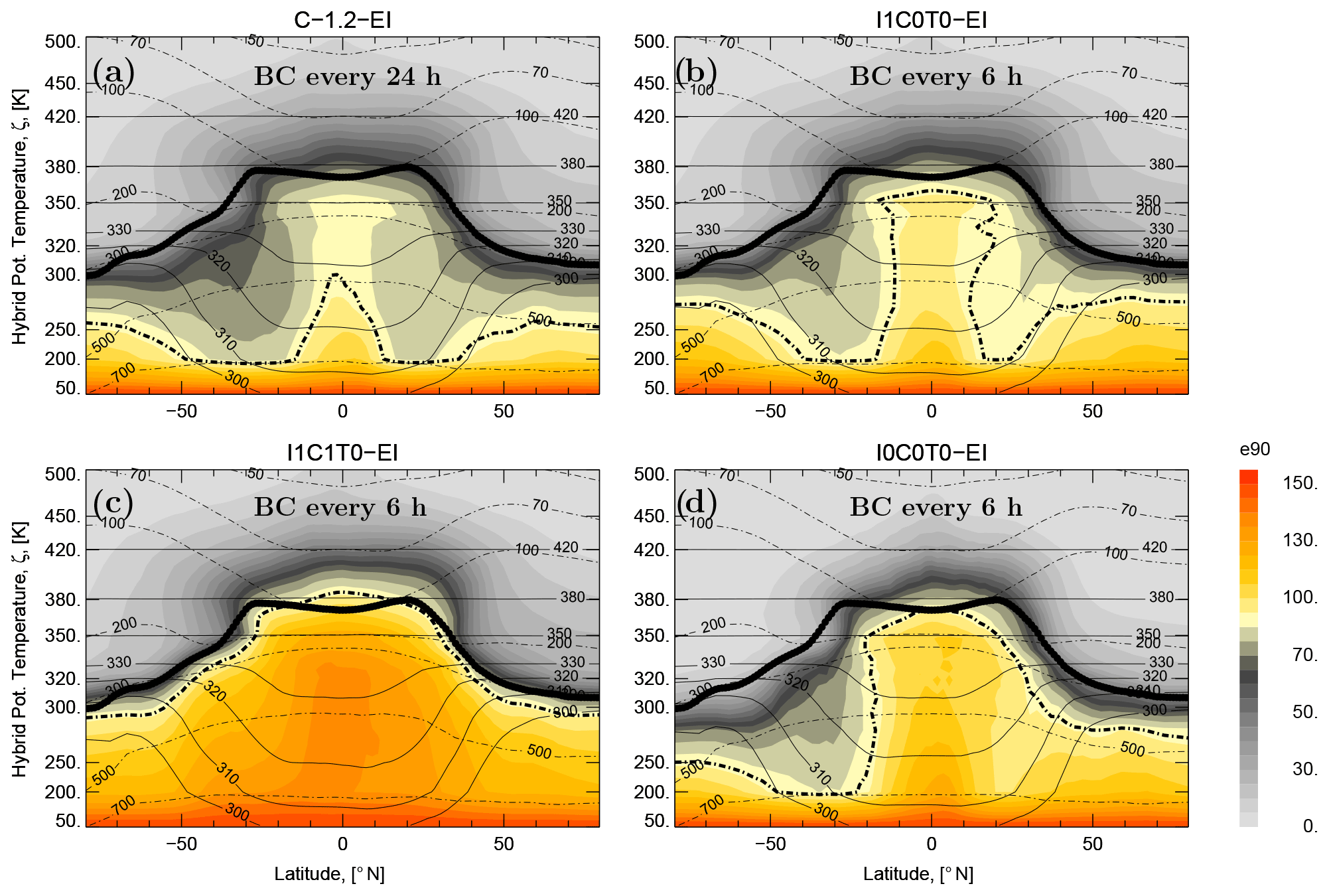
Figure 2Zonal and monthly mean (December 2017) of the e90 tracer distribution for four CLaMS/EI configurations: with only isentropic mixing in CLaMS 1.2 (a) and 2.0 (b), with isentropic mixing and unresolved convective updrafts in CLaMS 2.0 (c) and pure advection calculation in CLaMS-2.0 (d). In CLaMS 1.2 the boundary condition (BC) is updated every 24 h while in all CLaMS 2.0 configurations every 6 h. The black dashed and solid lines are the 90 ppbv isoline of the e90 tracer and the WMO tropopause, respectively.
In Fig. 2, four CLaMS/EI configurations are shown (zonal and monthly mean for December 2017). Isentropic mixing both in CLaMS 1.2 (Fig. 2a) and 2.0 (Fig. 2b) increases downward transport of stratospheric air into the troposphere if compared with pure advective transport (Fig. 2d). In the full extension of CLaMS 2.0 (Fig. 2c), there is the smallest distance between the e90 isoline and the WMO tropopause. Note that the same definition of the lowest layer approximating the PBL was used in the CLaMS 1.2 and 2.0 simulation (Fig. 2a and b). The only difference between these two runs is the update frequency of the boundary conditions (24 versus 6 h in the CLaMS 1.2 and 2.0, respectively). Thus, in CLaMS 2.0, the lowest boundary is reset more frequently (i.e., all APs in this layer are set to their default positions every 6 h) and, mainly in the tropics, the resolved convective uplifts can be better sampled increasing upward transport and shifting upwards the 90 ppbv isoline (Fig. 2b versus Fig. 2a).
An interesting feature can be seen when isentropic mixing is added to a pure advective transport (from Fig. 2d to b). The boreal winter isentropic mixing in the Northern Hemisphere (NH) seems to push down the 90 ppbv isoline, mainly in the extratropics where a strong bi-directional isentropic transport between the lowermost stratosphere and upper tropical troposphere is expected. Due to aging by (isentropic) mixing (Garny et al., 2014), the re-circulated air within the Hadley cell and within the lower branch of the Brewer–Dobson circulation in the NH becomes older, shifting downwards the 90 ppbv isoline, clearly seen in the NH and Southern Hemisphere (SH) subtropics. The reverse process, although significantly weaker, moves the 90 ppbv isoline upwards by in-mixing younger tropical air into the SH polar middle troposphere during the Austral summer. Finally, unresolved convection seems to work against the effect of aging by mixing and lifts the 90 ppbv isoline upwards into the region around the tropopause (Fig. 2c). At the same time, the meridional gradient across the Hadley cell becomes slightly weaker likely indicating maybe too strong contribution of convection in the extra-tropics. However, this point can be hardly validated due to lack of the respective experimental data.
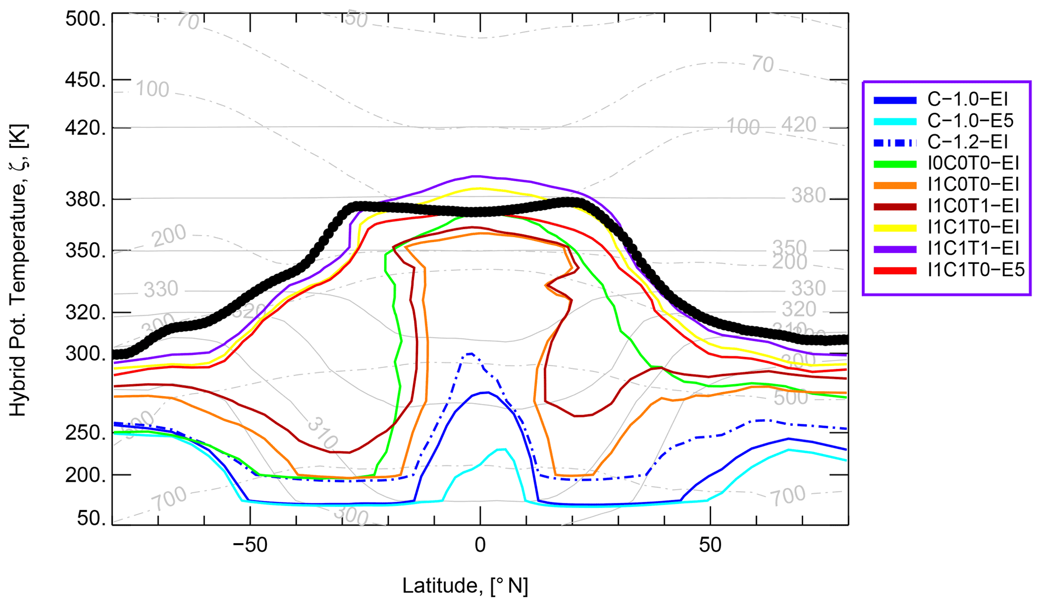
A more systematic comparison of all runs is shown in Fig. 3. The lowest 90 ppbv isoline can be seen for the C-1.0–E5 setup while the highest 90 ppbv isoline can be diagnosed for the EI run with all unresolved transport parameterizations switched on (i.e., I1C1T1). The largest deviation of the 90 ppbv isoline from the WMO tropopause can be diagnosed for the baseline runs with a small improvement by moving from the C-1.0 to C-1.2 configuration. The best e90 performance is obtained for the runs with isentropic mixing and unresolved convection (I1C1). If tropospheric mixing is additionally switched on (I1C1T1), the 90 ppbv isoline moves above the tropical tropopause suggesting too much upward propagation of tropospheric signatures in such a model configuration. Comparison with the pure advection run (I0C0T0) seems to perform better than the baseline runs and indicates that the effect of aging by mixing is either too strong or has to be compensated by other transport processes. One possible reason for a too strong isentropic mixing from the lowermost stratosphere into the tropical middle troposphere below ζ=350 K could be deviation of the model levels from the isentropes in this part of the atmosphere. Thus, CLaMS approximation of isentropic mixing confined by the model levels does not work correctly in this part of the atmosphere and may cause some spurious, cross-isentropic diffusion.
3.2 In situ observations: CO profiles
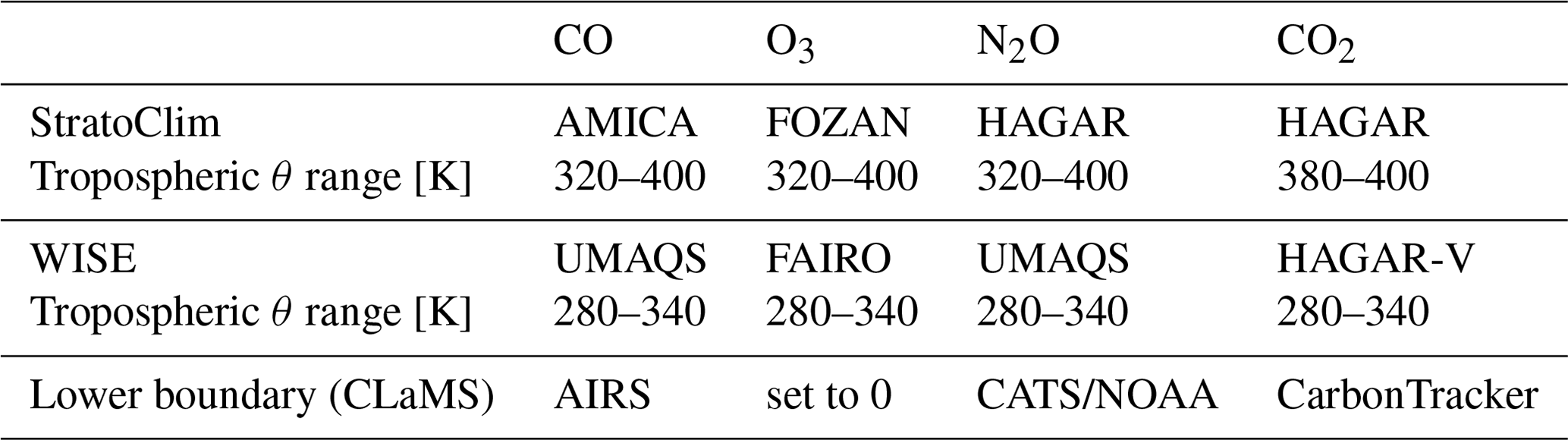
In the following, model results are compared to in situ data which were observed during the Geophysica campaign StratoClim (stratospheric and upper tropospheric processes for better climate predictions) in Nepal in July–August 2017 and during the HALO campaign WISE (wave-driven isentropic exchange) in Ireland in September–October 2017. While during StratoClim, tropical UTLS conditions within the Asian summer monsoon (ASM) anticyclone were sampled, WISE data represent much more extra-tropical and mid-latitude conditions in the vicinity of the subtropical jet. All CO, O3, N2O, and CO2 time series measured during these two campaigns are included (all local flights) with details listed in Table 3.
Table 3Observed species, instruments, and θ ranges included into the validation procedure, and the origins of the data used for the lower boundary condition in CLaMS (AIRS – atmospheric infrared sounder on NASA's Aqua satellite, Chromatograph for Atmospheric Trace Species (CATS) from NOAA, CarbonTracker from NOAA, version CT-NRT.v2017). For details of the CLaMS boundary conditions see Konopka et al. (2019) (CO2) and Pommrich et al. (2014) (all other species). Tropospheric θ ranges define maximal vertical extensions where new transport modes in CLaMS 2.0 are evaluated in terms of the root mean square differences between observations and model results. The instruments and their performance during StratoClim are described in von Hobe et al. (2021) and during WISE in Krasauskas et al. (2021) and Lauther et al. (2022).
All time series are transported to the closest 12:00 UTC synoptic time using CLaMS trajectories calculated with the same reanalysis as the respective CLaMS run. Tracer mixing ratios at the CLaMS air parcels closest to the observations quantify the model prediction (no interpolation from other potential neighbors).
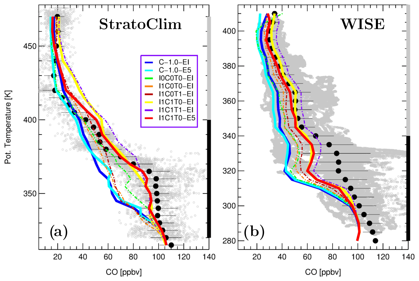
Figure 4All CO observations (gray) during the StratoClim (a) and WISE (b) campaigns are shown versus CLaMS simulations. The averaged experimental data are plotted as black bold symbols (mean values are calculated by gridding all observations and using an overlapping boxcar width). The respective results for the model runs are color-coded as described in the legend. For the baseline runs (C-1.0) and for the best runs (I1C1T0) thick solid lines are used. The root mean square differences calculated between the simulations and experimental data in the tropospheric range (black solid line on the right y axis) are listed in Table 4. The performance in the stratospheric range (gray solid line on the right y axis) is discussed in Sect. 3.6. Note the different y axis ranges in (a) and (b).
In Fig. 4, mean profiles of CO are plotted for each campaign and for different CLaMS setups listed in the legend. The mean observed CO profile during StratoClim (Fig. 4a) shows typical tropical features with highest values at the surface and around the main convective outflow between 360 and 370 K. Above this level, CO decreases, almost constantly, down to the stratospheric background above 420 K due to its chemical lifetime of the order of a few months (von Hobe et al., 2021). The root mean square differences calculated within the tropospheric ranges (see Table 3) quantify the performance of different CLaMS runs and are listed in Table 4.
A clear improvement in the model representation of the main convective outflow is achieved when unresolved convection is switched on (C1), and consequently the observed CO values around 90 ppbv between 360 and 370 K are reproduced by the model. As discussed in von Hobe et al. (2021), photolytic decay of CO in slowly ascending air within a well-confined ASM anticyclone defines the vertical gradient of CO between 365 and 420 K. Above this level, mixing with the surrounding stratosphere determines the CO mixing ratios. The vertical gradient of CO between 400 and 450 K is better represented in E5- than in EI-driven simulations (I1C1T0-E5 versus I1C1T0-EI). Tropospheric mixing (from I1C1T0 to I1C1T1) shifts CLaMS profile to too high values suggesting that this transport enhances the numerical diffusion rather than improves our simulations. Figure 4b shows mean CO profiles during WISE when mainly mid-latitude air was sampled. Comparison with CLaMS results confirms the importance of convection parameterization although CO values between 310 and 340 K are still underestimated. Remarkable is the CO minimum around 315 K which is much more pronounced in CLaMS simulations than in the observations. This difference between model and observations can either be explained by too much downward transport or not enough convective updrafts in the model.
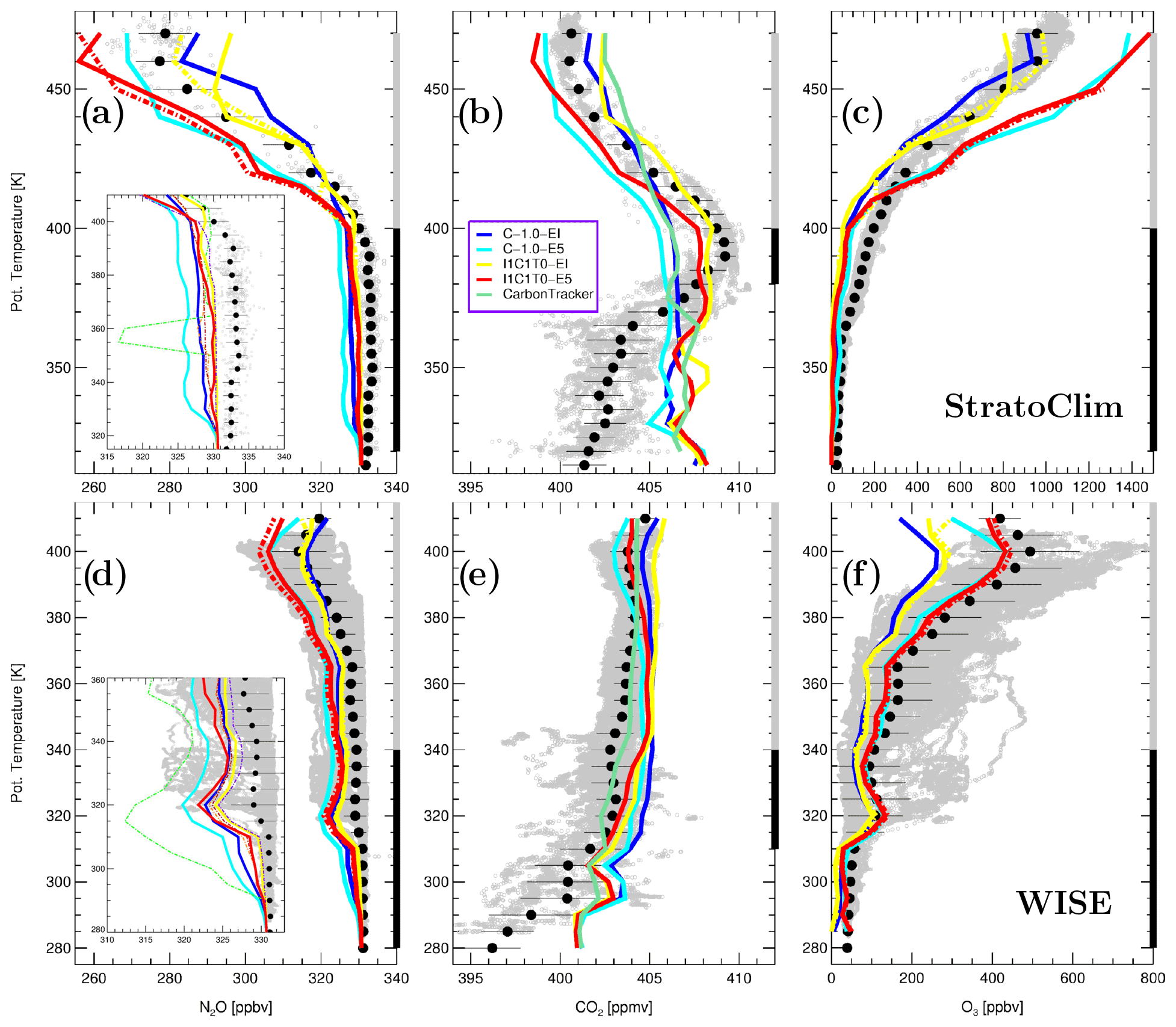
Figure 5Same as in Fig. 4 but for N2O (a, d), CO2 (b, e), and O3 (c, f) observations versus CLaMS for the most important model configurations listed in the legend of Fig. 4. For the baseline runs (C-1.0) and for the best runs (I1C1T0), thick solid lines are used. Dashed thick lines denote results of the respective perpetuum runs. Top and bottom panels show the StratoClim- and WISE-related profiles, respectively. CO2 profiles directly obtained from the CarbonTracker data are also shown (beige green). In the subpanels for N2O, details of tropospheric profiles are higher resolved and color-coded as in Fig. 4. Table 4 compares the root mean square differences and Sect. 3.6 discusses the stratospheric performance within the tropospheric and stratospheric ranges, respectively.
3.3 N2O, CO2, and O3 profiles
Now we compare in Fig. 5 the same type of mean profiles like for CO (Fig. 4) but for N2O and CO2 which are tropospheric tracers with much longer lifetimes than CO (∼ 100 yr for N2O and even centuries for CO2). Below the tropopause, N2O does not show much variability and can be characterized by a weak positive and negative mean vertical gradient for the StratoClim and WISE data, respectively (Fig. 5a and d). The deviation of the simulated from the observed gradients measures the quality of the CLaMS runs; for a more detailed, zoomed view see the subpanels of Fig. 5a and d. Note that the pure advection run (I0C0T0) shows the worst performance with few very low (unmixed) stratospheric values in the lower troposphere. The best performance can be diagnosed for the runs with isentropic mixing and unresolved convection (I1C1) or even I1C1T1-runs, where tropospheric mixing was added. Note also a layer around θ=320 K in the extratropical WISE data (Fig. 5d) with low N2O values marking signatures of stratospheric intrusions. This layer is much more pronounced in CLaMS simulations than in the observations, and is consistent with a similar feature in CO profile (Fig. 4b).
Mean CO2 profiles (Fig. 5b and e) can be understood as a result of a coupled tropospheric and stratospheric transport folded in time and space with the evolution of the CO2 sources (and sinks) in the PBL while both transport and sources show a pronounced seasonality (Diallo et al., 2017). CO2 being almost chemically inert is a well-suited tracer for validation of transport in the models if the lower boundary condition is realistically parameterized. However, the (assimilated) CarbonTracker data set used for the lower boundary of CLaMS does not reproduce well the CO2 observations in the lowest part of the troposphere where air dominated by regional sources was sampled (Kathmandu/Nepal for StratoClim and Shannon/Ireland for WISE). These special regional conditions which are not well-resolved in the CarbonTracker data (thick green line in Fig. 5b and e) are becoming less important around the tropopause where global rather than regional source regions contribute to the observed CO2 mixing ratios. Ray et al. (2022) have shown that during the summer monsoon season over North America, the observed CO2 profiles above 380 K are influenced rather by tropical than regional sources and even dominated by such sources above 420 K.
Thus, we compare now the observed mean profiles of CO2 with CLaMS simulations only above θ larger than 380 and 310 K for StratoClim and WISE observations, respectively. First, the upward propagation of the CO2 seasonal cycle during StratoClim is better reproduced in the CLaMS 2.0 version including parameterization of unresolved convective updrafts and improved boundary conditions (I1C1T0-EI/E5) compared to the former model version CLaMS 1.0 (C-1.0-EI/E5) and even better than by the CarbonTracker data set as can be deduced from the comparison around θ=380 K. Second, above this level, the upward propagation of the CO2 signal is rather too fast in the EI-driven simulation and too slow for the E5 meteorology in some agreement with our CO-related results. The same type of behavior can also be diagnosed during WISE with a better performance of CLaMS 2.0 in the tropospheric regime between 310 and 340 K. Note that 1 yr simulations (2017) limit the interpretation of the upward propagation of the CO2 signal, and results of the perpetuum run cannot be applied because of a too strong positive CO2 trend in the PBL.
Finally, O3 profiles are shown in Figs. 5c and f. In the mid-latitudes during WISE, O3 gradients are better reproduced in the E5-driven runs while mean profiles of N2O are better represented by the EI-driven simulations. Because only a simplified O3 chemistry is used (Pommrich et al., 2014) and the upper boundary of O3 is defined at θ=500 K by HALOE climatology, CLaMS results should be interpreted with caution. Especially, some missing chemical loss or production cycles of O3 may be the reason for a wrong interpretation of the vertical gradients of ozone. The low bias of O3 below 410 K during StratoClim is only partially related to our lower boundary condition setting O3 to zero and more likely caused by the pollution-induced ozone production in the monsoon anticyclone which is not represented in the model.
3.4 CO–O3 correlation
A convenient diagnostic of transport in the UTLS offers the CO–O3 correlation observed in the UTLS (Hoor et al., 2002; Pan et al., 2004; Kunz et al., 2009). In the CO–O3 space, this correlation is characterized by CO and O3 branches defining the (mean) troposphere and stratosphere, respectively, and by the remaining part sampled in the UTLS region (Fig. 6). In the extratropical UTLS, this part is formed mainly by isentropic mixing in the vicinity of the jets (Konopka and Pan, 2012) while in the tropical tropopause Layer (TTL), photochemistry rather than isentropic mixing is the reason (Vogel et al., 2011; von Hobe et al., 2021). To focus on mixing processes close to the subtropical jet, we include only WISE data in the following analysis.
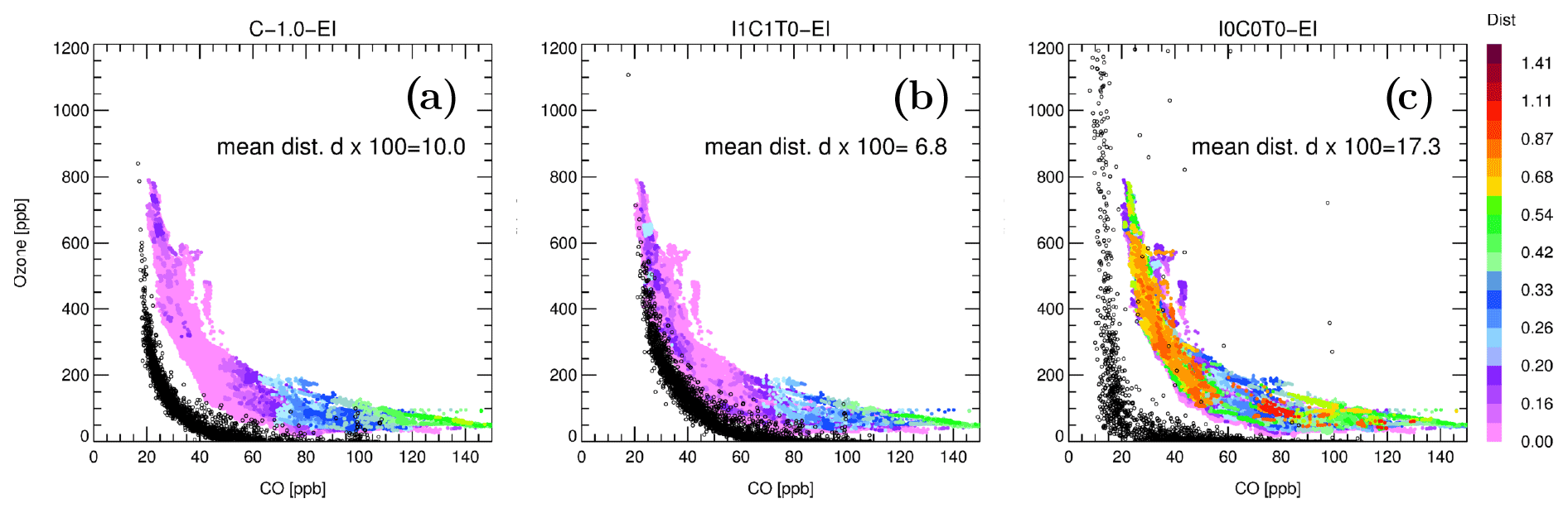
Figure 6CO–O3 correlation-based metrics. Observed (colored) versus simulated (black) CO–O3 correlation for all flights of the WISE campaign. The observed data are color-coded with the mean (Euclidean) distance d (dist) calculated in the CO–O3 space after normalizing CO and O3 data by 200 and 3000 ppbv, respectively. With denoting the square of the Euclidean distance between the observed (“o”) and simulated (“s”) (normalized) CO/O3 () value pairs i; d is defined as the arithmetic mean over all di values. Note that d is a dimensionless quantity varying between 0 and (here multiplied with 100). (a) Baseline run (C-1.0-EI), (b) isentropic mixing and unresolved convection (I1C1T0), and (c) pure advection (I0COT0).
A comparison between the observed and simulated CO–O3 correlation is shown in Fig. 6, exemplarily for three EI-driven CLaMS configurations: CLaMS 1.0 baseline run (Fig. 6a), CLaMS 2.0 including isentropic mixing and unresolved convective updrafts (Fig. 6b), and for the pure advection run (Fig. 6c). In a perfect model, the observed and simulated correlations should be equal. Deviations from such an idealization can be used to evaluate the model transport representation. Here, following the procedure described in Konopka et al. (2004) to optimize the CH4–H1211 correlation, a mean (Euclidean) distance d calculated in the normalized CO–O3 space is used to measure such deviations (for exact definition, see caption of Fig. 6). Note that the observed correlation shown in all panels of Fig. 6 is always the same although colors over-plotting this correlation are different due to different distances between the simulated (black) and observed (color-coded) correlations.
To reconstruct correctly the observed CO–O3 correlation, both the end members of the mixing lines and the isentropic mixing itself should be well-represented in the model. Especially the CO values of the air parcels undergoing isentropic mixing in the model are preconditioned by the representation of convection in the model. In this way, the CO–O3 correlation-based metric rates not only isentropic mixing but also the quality of the other transport modes like parameterized unresolved convection or tropospheric mixing. As discussed in Pan et al. (2006), missing isentropic mixing in pure advective studies explains a poor representation of the observed CO–O3 correlation (Fig. 6c). Thus, CLaMS 1.0 configuration (Fig. 6a) including isentropic mixing performs better, with smaller d values as in Fig. 6c. The CLaMS 2.0 run (I1C1T0, Fig. 6b) gives in this example the smallest d value, i.e., the best representation of the observed CO–O3 correlation, by combining unresolved convective drafts with isentropic mixing.
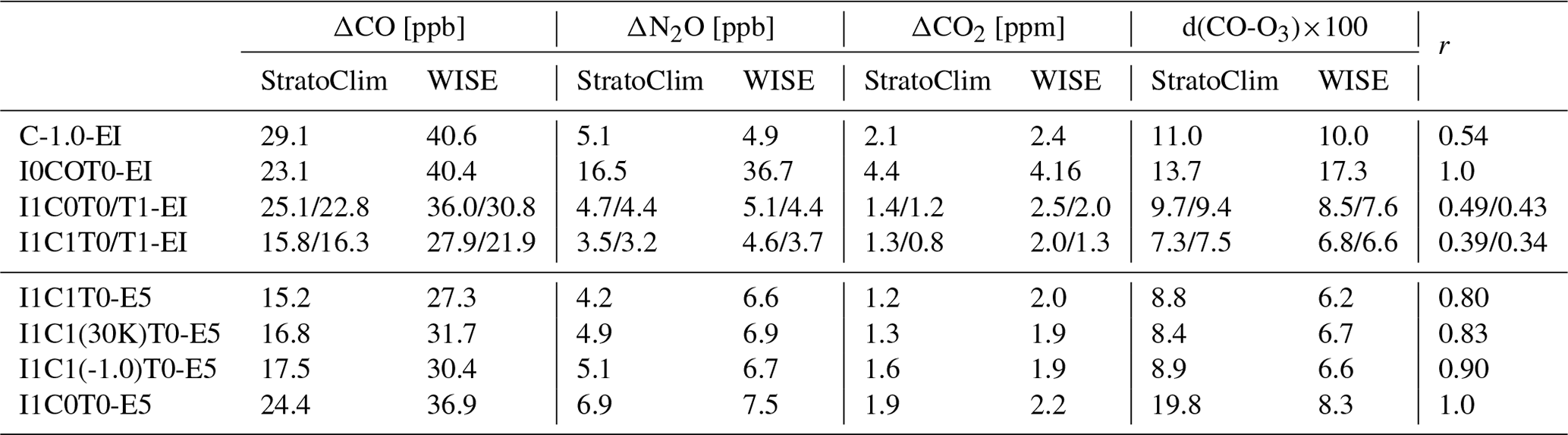
Table 4Rating of the EI- and E5-driven runs (upper and lower parts of the table) in terms of the root mean square differences Δ calculated over the vertical ranges listed in Table 3 and in terms of the mean deviations d from the observed CO–O3 correlation during StratoClim and WISE (smallest values of Δ an d indicate the best performance). These four metrics mi are normalized by their maximal values within each of the considered group and are used to calculate the cumulative rating parameter r defined as a sum of all metrics mi normalized by the sum maximum (i.e., r=1 means the worst case and smallest value of r means the best case). While for the first four cases (EI runs), r is calculated relative to the pure advection case (I0COT0-EI), and r value of the last four cases (E5 runs) are determined relative to the pure isentropic run (I1C0T0-E5).
3.5 Rating of different transport scenarios
Table 4 summarizes the rating of all runs, both in terms of the root mean square differences and by using the parameter d discussed above. With exception of CO, pure advection runs show by far the worst performance. For CO, CLaMS 1.0 is the worst case mainly because the update frequency of the lower boundary condition is lower in CLaMS 1.0 than in the pure advection run (24 versus 6 h, see also discussion related to the Fig. 2, a slightly thinner lower boundary compared with CLaMS 2.0 runs plays only a minor role). To compare all EI-related results (upper part of Table 4), the cumulative rating parameter r was determined (for exact definition, see caption of Table 4) with r=1 quantifying the worst case (pure advection) and with the smallest values of r pointing to our best cases (last column in Table 4). We conclude that the largest improvement was achieved by including isentropic mixing in the model simulation (I1 versus pure advection I0). The second largest improvement results by adding to isentropic mixing the parameterization of the unresolved convective uplifts. By including tropospheric mixing (numbers behind the slash), only weak improvement was found. Note that the best E5-driven run (I1C1T0-E5) performs slightly better than the respective EI simulation (I1C1T0-EI) in terms of ΔCO, ΔCO2, and d (WISE) but not in terms of ΔN2O.
Finally, to further illustrate the contribution of unresolved convective uplifts to transport in the troposphere, we analyze differences in the vertical distribution of air parcels in CLaMS for configurations with same isentropic mixing but different strengths of parameterized convection (i.e., for I1C1T0 runs). For this reason, forward E5-driven trajectories are globally started, every 6 h, from the CLaMS PBL uniformly covered by about 68 000 air parcels (APs). The time length of every trajectory is also 6 h. Positions at the start and at the end of every trajectory are used to calculate Δθ of air parcels lifted upwards. The first 10 d (i.e., almost 40 time steps) of January 2017 are considered. We compare the run I1C1T0-E5 (which performs similarly well as the I1C1T0-EI run) with runs where the convection parameterization was reduced (I1C1(30K)T0, I1C1(-1.0)T0-E5) or even completely switched off (I1C0T0).
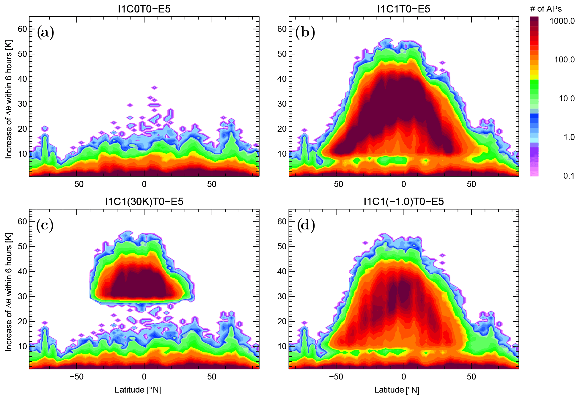
Figure 7Total number of APs lifted upwards (units: total number per lat/theta grid size and time step) in different E5-driven configurations averaged over the first 10 d of January 2017. (a) Run without any convective parameterization. (b) Run with the parameterization of unresolved convection and with the best agreement with experimental data. (c, d) Two sensitivity studies for unresolved convection with Δθc>30 K (instead of Δθc>10 K, a, c) and for 1 s−2 (instead of 1 s−2, right).
Figure 7 shows such a comparison using the total number of the uplifted air parcels as a function of latitude and the uplift Δθ averaged over all (advective) time steps while Table 4 (lower part) compares these runs using metrics discussed above. Both sensitivity runs perform worse compared with the best case. Starting from a pure isentropic run I1C0T0 as a reference with the cumulative metrics equal 1 (worst case), the improvement of the runs with convection can be quantified by 0.90, 0.83, and 0.80 for the I1C1(-1.0)T0, I1C1(30K)T0, and the best run I1C1T0, respectively The comparison with the run without any parameterization of convection (Fig. 7a) shows that a massive redistribution of APs is necessary (from d, c, to b) in order to reproduce the observed features like the main convective outflow in the CO/N2O profiles.
3.6 Stratospheric performance
Because CLaMS 2.0 runs cover only 1 yr, the impact of the new tropospheric transport modes on the composition of tracers in the stratosphere is not well-resolved. For such studies, transient runs of the order of 10 yr would be necessary to correctly reproduce the old air masses. Here, CLaMS 2.0 perpetuum runs for 2017 are used to mimic such transient runs. Furthermore, the simulated tracer distributions in the stratosphere are mainly determined by the representation of the Brewer–Dobson circulation (BDC) in the reanalyses and are well-documented for the EI (Ploeger et al., 2019) and E5-driven (Ploeger et al., 2021) multi-year CLaMS 1.0 simulations. While EI-driven runs show a too fast BDC, with too young air masses in the tropical lower stratosphere, the reverse effect was diagnosed for the E5-driven runs with rather too slow BDC and too old air in the TTL. These findings are consistent with stratospheric parts of the simulated O3 and N2O profiles shown in Fig. 5 (thick dashed lines for the perpetuum runs). Thus, in the tropical stratosphere above 400 K during StratoClim, E5-driven runs seem to produce too strong stratospheric gradients of O3 and N2O profiles while the EI-based simulations compare better with the observations.
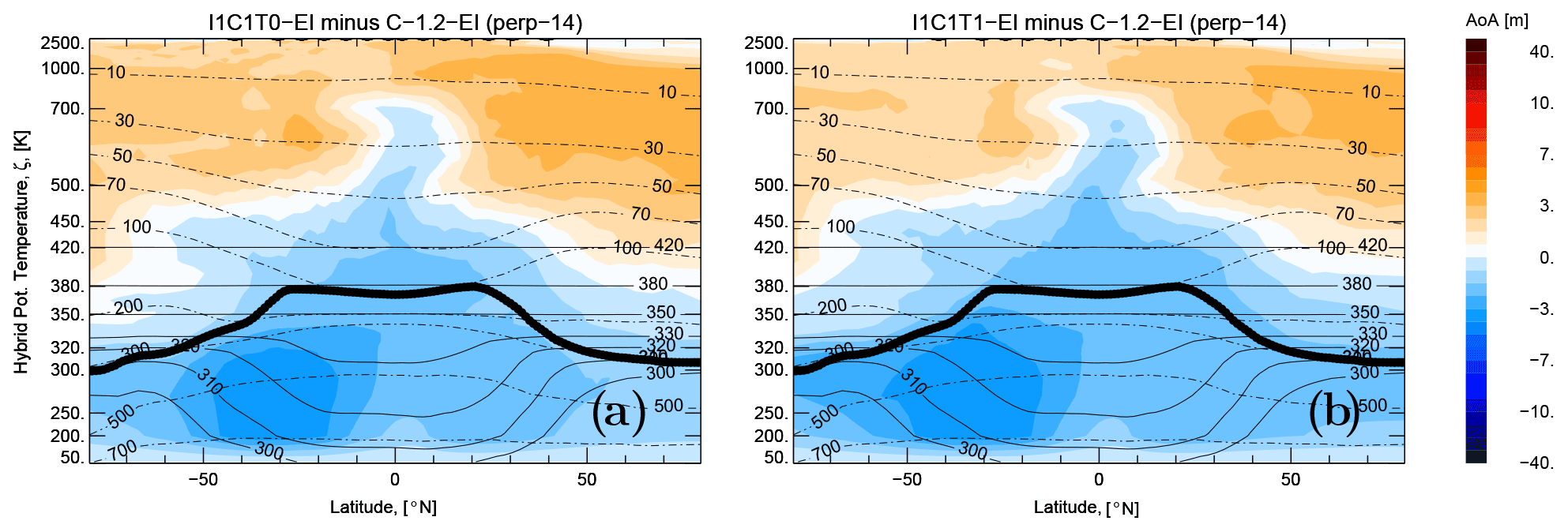
Figure 8Impact of tropospheric transport modes on the distribution of the age of air (AoA) (in months) shown as a difference to the CLaMS 1.2 AoA distribution (December 2017, perpetuum 14 yr): with unresolved convection (a), and with unresolved convection and tropospheric mixing (b). The results for the respective E5-driven simulations are very similar in the troposphere; the stratospheric effect of aging by mixing is even weaker (not shown).
We discuss now how the tropospheric modes of transport implemented in CLaMS 2.0 influence the distribution of the age of air (AoA). Figure 8 shows that tropospheric air becomes younger for runs including unresolved convection (Fig. 8a) and even younger if tropospheric mixing is added (Fig. 8b). The strongest effect is diagnosed in the middle troposphere around 40∘ S and reflects the seasonality of convection shown here for December 2017. The rejuvenation of air propagates upwards into the tropical pipe and covers the whole lowermost stratosphere below θ=380 K. Above this level, re-circulation and aging by mixing (Garny et al., 2014) makes the air older due to slightly changed intensity of isentropic mixing in CLaMS 2.0 compared with CLaMS 1.0, although the relative values of these changes are small.
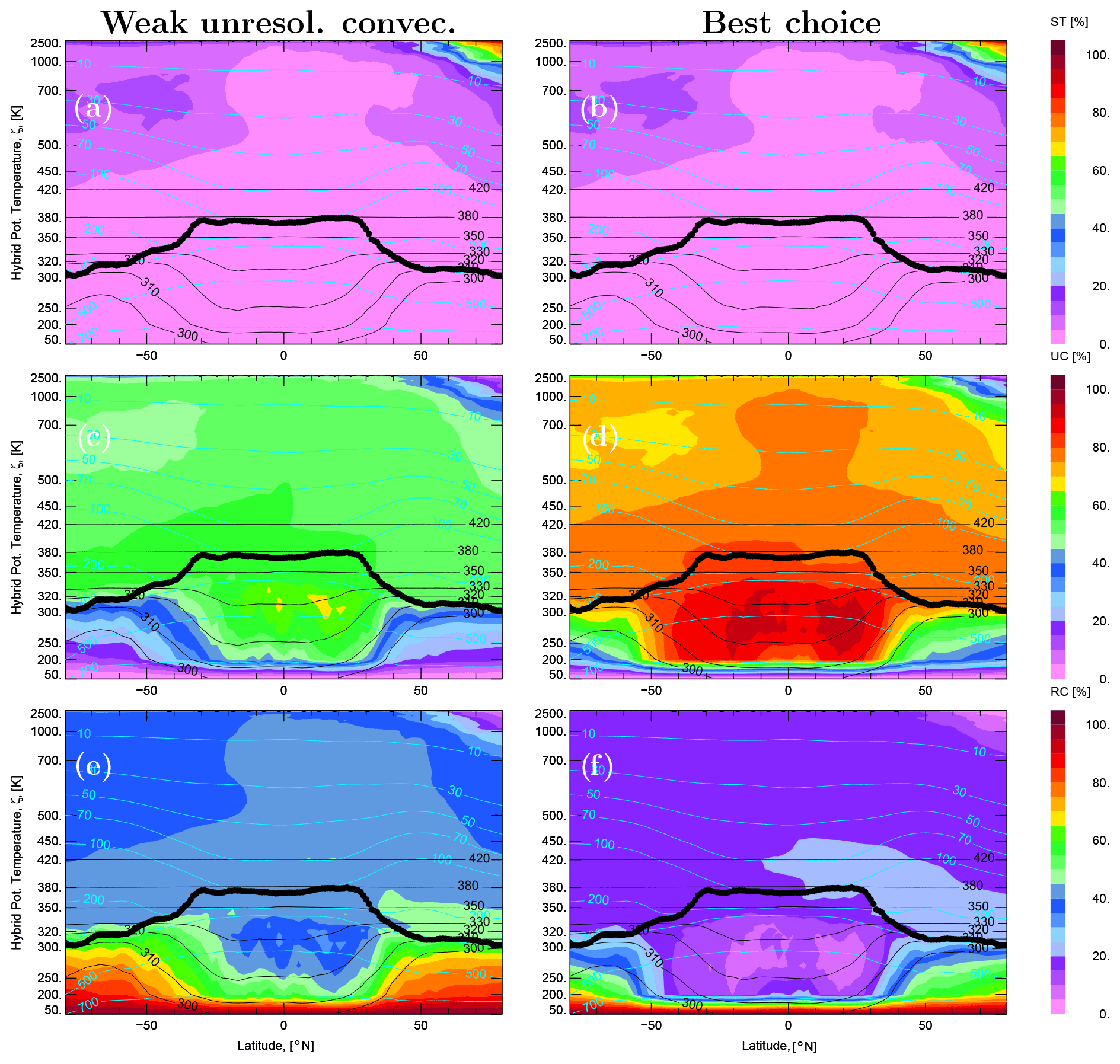
Figure 9Budget of three origin tracers quantifying the contributions of the upper boundary (stratosphere (ST) panels a and b) and of the lower boundary of CLaMS (unresolved convective updraft (UC) and transport resolved in ERA5 (RC) shown in panels (c) and (d), and (e) and (f), respectively). ST, UC, and RC are calculated for the last day of the 14 yr perpetuum run (31 December 2017) for the weak contribution of the unresolved convection (left column, run I1C1(-1.0/30K) T0-E5) and for the best case (right column, run I1C1T0-E5). By repeating 14 times year 2017, a steady state with respect to these tracers was reached, i.e., ST + UC + RC = 100 %. With lower boundary approximating the PBL, UC quantifies the contribution of unresolved convective updrafts and RC the contribution of the PBL following the transport resolved in the ERA5 reanalysis.
The unresolved convection strongly influences the pathways of air into the stratosphere. For further illustration, idealized tracers denoted as ST and TR are released in the upper and lower boundary of CLaMS, respectively. The zonal mean of their spatial distribution is calculated for the last day of the 14 yr perpetuum run (31 December 2017) and shown in Fig. 9. In addition, TR is divided into two subsets, UC quantifying the contribution of the unresolved convective updrafts and RC measuring the amount of air which does not experience any parameterized updrafts. All three tracers add up to 100 % and quantify the amount of air following different pathways: from the top of the stratosphere (ST), from the Earth's surface via the unresolved convective updrafts (UCs) and from the other Earth's sources following the transport resolved in ERA5 (RC). Note that by switching off the convection parameterization, UC = 0 is valid. As can be seen in the left column of Fig. 9, even a weak contribution of convection parameterization leads to UC values around 50 % between the tropopause and ∼50 hPa. However, in order to reproduce the observed tropical main convective outflow like that diagnosed in the StratoClim CO observations, much stronger contribution of unresolved convective updrafts is necessary (best case, second column in Fig. 9), indicating UC values around 75 % in the lower stratosphere. We conclude that it is very unlikely to transport air from the boundary layer into the stratosphere following only the pathway with convection resolved by the reanalyses.
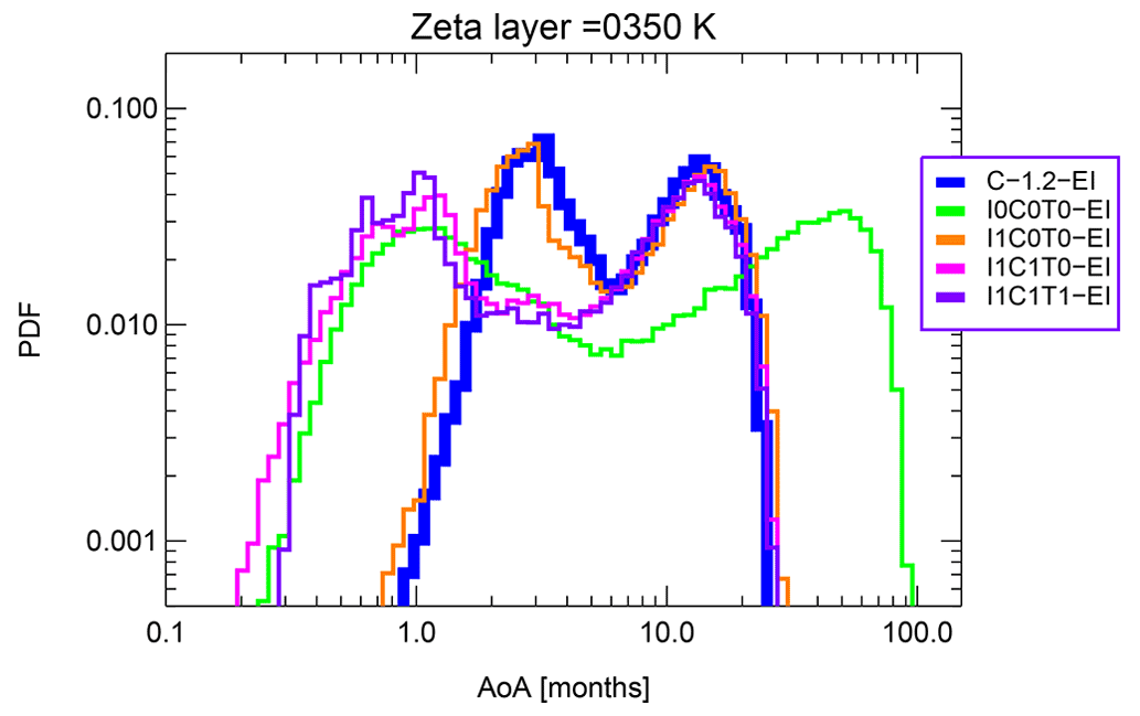
Figure 10The probability distribution functions (PDFs) of age of air (AoA) after 14 yr of perpetuum runs averaged over all APs within the CLaMS layer around ζ=350 K.
To visualize how much younger the air in the UTLS region is if tropospheric modes of transport are switched on, the probability distribution functions (PDFs) of AoA are compared in Fig. 10 for different EI-driven model runs. These PDFs are calculated for all air parcels within the CLaMS layer around ζ=350 K for the last day (31 December 2017) of the respective perpetuum run. Two modes in Fig. 10 should be distinguished: a tropical mode in the upper troposphere on the left which is mainly affected by the convection and an extra-tropical mode in the lower stratosphere on the right which is mainly affected by isentropic mixing. As intended, there is no significant difference between the pure isentropic CLaMS 2.0 run (I1C0T0) and the reference run C-1.2. Including unresolved convection (C1T0) or unresolved convection and tropospheric mixing (C1T1) significantly enhances the contribution of young air to the air composition around ζ=350 K. This is even slightly more than pure advection (I0C0T0) can provide. In addition, pure advection transport produces very old air which, as shown in the previous section, does not match experimental data. This picture does not significantly change up to ζ=400 K where both maxima merge for all runs with exception of the pure advection.
Finally, we discuss the robustness of our findings. Certainly, our parameterization of unresolved convective updrafts can be improved by increasing its frequency from every 6 to every 1 h (E5 reanalysis is available every 1 h), by replacing our parameters triggering the onset of convection (, Δθc, see Table 1) with CAPE (convective available potential energy) widely used in the meteorological and climate community, or by including the diurnal cycle of the PBL depth. All these potential improvements could follow the methods used in the respective reanalysis driving CLaMS (here EI or E5) making the parameterization of convection more consistent with the underlying advective winds. On the other side, such an approach would strongly depend on the used reanalysis (every reanalysis has its own convection scheme), and consequently would be less suitable to be implemented into climate models. Thus, although our results are rather qualitative, we do not expect that a better convection scheme improving the representation of unresolved convective updrafts and downdrafts would significantly change the importance of this process in the transport from the PBL into the stratosphere as shown in Fig. 9. However, the impact of such an improved scheme on the position and the shape of the tropical mode shown in Fig. 10, i.e., on the timescales of transport from the PBL to the upper troposphere, can be more essential.
Similarly, our results related to the dominance of the isentropic mixing are rather qualitative than quantitative. Although by moving from CLaMS 1.0 to 2.0 the numerical values of the mixing parameters (λ, ϵ and the mixing frequency Δt, see Table 1) have changed, the mixing intensity defined as the number of mixing events per time unit and its spatial distribution are very similar. The climatologies of the mixing events show for both versions similar properties with enhanced isentropic mixing around the jets and within the TTL, and smallest mixing activities in the summer extra-tropical stratosphere where the solid body rotation with a negligible amount of local strain dominates the flow (Piani and Norton, 2002). The minor importance of tropospheric mixing found in our study still needs further investigation after improving the representation of the PBL in the model (see above).
An interesting question is the dependence of our results on the spatial (and temporal) resolution of the underlying reanalysis especially by including the highest available spatial and temporal resolution of E5 meteorological data (i.e., time resolution = 1 h, spatial resolution ∼30 km in contrast to 6 h and ∼100 km used in this study). The more precise question is how much of the unresolved convection presented in this study could be resolved by using such high-resolution version of the meteorological data. On the contrary, it is virtually certain that mixing signatures like those observed in the CO–O3 correlations cannot be provided by pure forward trajectory calculations making (isentropic) mixing indispensable (Pan et al., 2006) although the dependence of the mixing parameters on the model resolution also needs further investigations.
Including unresolved tropospheric transport processes like convection and mixing, as implemented in the newly released CLaMS model version (CLaMS 2.0), improves tracer representation of the UTLS in the model. While the parameterization of unresolved convection enables reproducing the signatures of the main convective outflow as observed in the tropical CO profiles, the potential improvements related to the parameterization of tropospheric mixing in CLaMS 2.0 are less obvious. As deduced from the in situ-based metrics, tropospheric mixing seems to remove some tropospheric variability in the simulated N2O profiles and to homogenize vertically these profiles, in some agreement with the observations. On the other hand, the e90-based tropopause is slightly too high in the tropics and the comparison with the CO profiles within the ASM anticyclone indicates also a too strong contribution of tropospheric mixing.
Although both parameterizations, i.e., those of unresolved convection and of tropospheric mixing, only weakly influence the stratospheric distribution of mean age of air, their influence on the young part of the age spectrum and therefore on the very short-lived substances (VSLS) like the ozone-depleting, halogen-containing substances is still not quantified. Especially the parameterization of unresolved convection strongly influences the potential pathways of transport from the Earth's surface not only into the UTLS region but also into the whole stratosphere. The dominant contribution of the convective pathway, i.e., from the boundary layer via the main convective outflow into the stratosphere (see Fig. 1), to the composition of stratospheric air highlights the importance of a reliable convection parametrization in the global climate models.
The Lagrangian (irregular) grid of air parcels (APs) in CLaMS covers the whole atmosphere from the surface to around 50 km or ζ=2500 K with ζ being the hybrid potential temperature (Mahowald et al., 2002). The initial positions of APs are generated following the concept described in Konopka et al. (2012) (i.e., by assuming that the aspect ratio is controlled by the static stability and that the entropy of the system is uniformly distributed over all APs). However, this concept, mainly developed for the free atmosphere, may be not valid in the vicinity of the Earth's surface where atmospheric transport is dominated by the boundary effects like friction and convection. Thus, we decouple the horizontal and vertical resolution of the lowest model layer (approximating the planetary boundary layer (PBL)) from the grid generation procedure in the sense that both the vertical and horizontal separation of the APs in this layer can be freely chosen (Fig. A1).
Isentropic mixing of APs in CLaMS is based on the adaptive grid procedure with interpolations triggered by flow deformations detected layer-wise during each advective time step Δt. The APs covering the whole atmosphere are divided into layers which are parallel to isentropes roughly above pr=300 hPa. The model layers directly above the Earth's surface follow the orography rather than isentropes. In every layer, the adaptive grid procedure inserts and merges APs in the regions of strong flow deformations. Let r0 be the mean separation between the APs in an arbitrary chosen layer. Then, two critical distances, r±, are defined as , with the Lyapunov exponent λ parameterizing critical deformation triggering adaptive interpolations after inserting () or after merging () of the APs. In general, the adaptive grid procedure increases the total number of APs up to 50 % relative to the initialization (in particular layers, this number is even higher). Especially in the deformation-dominated zones, like outer flanks of the jets (e.g., polar or subtropical jets) or in the tropical stratosphere within the quasi-biennial oscillation (QBO) wind reversal, a temporal increase of APs number can be diagnosed. Thus, the merging step of the adaptive grid procedure balances the deformation-induced insertion of new APs and keeps the total number of APs within a certain range (Fig. A2).
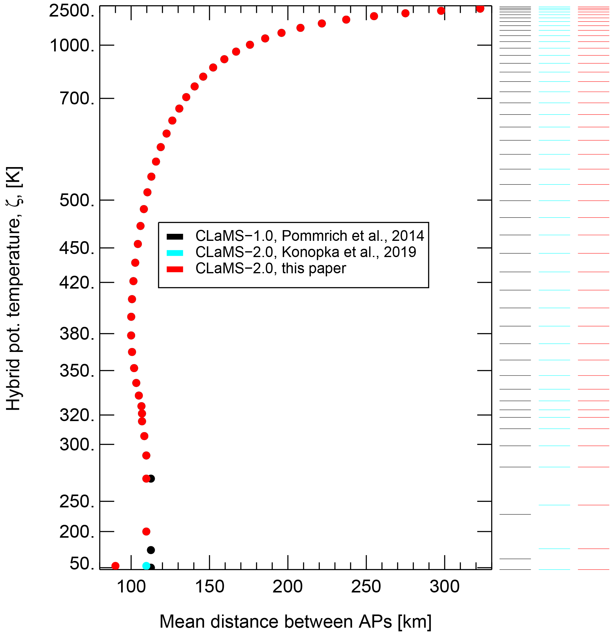
Figure A1Initial distribution of APs with slightly enhanced thickness of the lowest layer (from ζ=100 to 140 K, i.e., from CLaMS 1.0 to CLaMS 2.0) and with slightly increased horizontal resolution in this layer used here (r=90 km instead of r=110 km) for grid configuration generated with r0=100 km and aspect ratio α=250 at ζ=380 K following procedure described in Konopka et al. (2012). For the here used EI/E5 reanalyses, the zonal horizontal resolution varies between 111 km at the Equator and 78 km at 45∘ latitude. With the choice r=90 in the lowest layer, we aim to better include the resolved tropical convective updrafts.

Figure A2Starting with the initial distribution of APs (1 January 1979, baseline run), their total number increases in the CLaMS 1.0 standard configuration during the first 2 weeks of the simulation for both EI (solid) and E5 (dashed) cases (a). Panel (b) shows the numbers of APs after mixing step due to insertion (lower branch) and due to merging (upper branch). A steady state is reached after about 10 d. Note that the number of merged APs is always larger than the number of inserted APs. This is because a large part of inserted APs is subsequently merged, and consequently counted as merged and not as inserted.
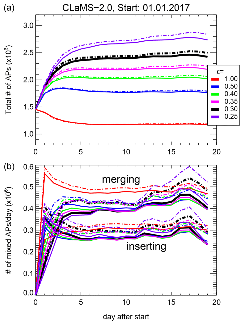
Figure A3Tuning of ϵ for runs with Δt=6 h, λ=4.0 d−1. Here different values of ϵ are used, from ϵ=1 (CLaMS 1.0) to ϵ=0.25. To get the total number of APs which is similar to that in CLaMS 1.0 reference run, ϵ=0.3 is recommended (black). Solid and dashed lines denote the EI- and E5-driven runs, respectively.
In CLaMS 2.0 shorter advective time steps Δt are applied in order to resolve the diurnal cycle of unresolved convection (6 instead of 24 h in CLaMS 1.0). For a better control of the adaptive grid procedure, we redefined r− to , with ϵ regulating the intensity of merging keeping the total increase of APs (relative to the initial value) below around 50 %. The use of the parameter ϵ is new. Typical values are around 0.30 for Δt=6 h and λ=4.0 d−1 although other choices are possible and need further investigation (Fig. A3). The choice ϵ=1 with Δt=24 h restores CLaMS 1.0 configuration. Parameterization of convection within CLaMS 1.0 configuration works only with Δt=24 because convection and mixing frequency must be equal in order to follow the relative motion of all advected APs.
The need of using ϵ<1 is obvious for Δt=6 h. For such configurations, the elimination step (with ϵ=1) is too strong compared with the insertion step. Consequently, the total number of APs decreases from the initial configuration by more than 50 % (Fig. A3, red line). Although it is possible to start the model with respectively larger number of APs, it is advantageous to enhance the number of APs in strongly deformed parts of the flow where tracer filaments and small-scale structures are very likely and where higher density of APs can better resolve their structures. Using the parameter ϵ, it is possible to tune the model in order to increase the model resolution in the mixing zones.
MESSy is continuously further developed and applied by a consortium of institutions. The usage of MESSy and access to the source code is licensed to all affiliates of institutions which are members of the MESSy Consortium. Institutions can become a member of the MESSy Consortium by signing the MESSy Memorandum of Understanding. More information can be found on the MESSy Consortium Website (http://www.messy-interface.org, last access: 30 June 2022). The CLaMS-2.0/MESSy code presented here is based on MESSy version 2.54 and accessible for MESSy Consortium members at https://gitlab.dkrz.de/MESSy (last access: 1 October 2021). ERA5 and ERA-Interim model level reanalysis data are available from the ECMWF as deterministic forecasts (atmospheric model): ERA5 via https://apps.ecmwf.int/data-catalogues/era5/?class=ea (last access: 1 January 2022) and ERA-Interim via https://apps.ecmwf.int/archive-catalogue/?class=ei (last access: 1 January 2022). The CarbonTracker data (version CT-NRT.v2017) can be downloaded from the NOAA ftp server: http://ftp.cmdl.noaa.gov, see: /products/carbontracker/co2/CT-NRT.v2017/molefractions/co2_total/. The StratoClim and WISE data can be downloaded from the HALO database at https://halo-db.pa.op.dlr.de/mission/101 (last access: 1 August 2022) and at https://halo-db.pa.op.dlr.de/mission/96 (last access: 1 August 2022), respectively. For more detailed model data, please contact the authors.
PK, FP, MT, and MvH conceived the presented ideas. PK performed the numerical simulations and wrote the paper. LH contributed with his experience related to convection parameterization and to the high-resolution ERA5 data. CK, MvH, FR, CMV, VL, AZ, and PH provided and helped to use the experimental data obtained during the StratoClim and WISE campaigns. All authors contributed to finalizing the paper.
The contact author has declared that none of the authors has any competing interests.
The European Centre for Medium-Range Weather Forecasts (ECMWF) provided meteorological analysis for this study. We thank Alexey Ulanowski and Vladimir Yushkov for their support related to the O3 FOZAN data. Excellent programming support was provided by Nicole Thomas. The authors gratefully acknowledge the project CLaMS-ESM of the Earth System Modelling Project (ESM) for funding this work by providing computing time on the ESM partition of the supercomputer JUWELS at the Jülich Supercomputing Centre (JSC). Jens-Uwe Grooß and Gebhard Günther strongly contributed to the data management on the supercomputer. We also thank Johannes Wintel and Thorben Beckert who supported HAGAR operations and data analysis during StratoClim, as well Johannes Wintel, Andrea Rau, and Emil Gerhardt for their support with the HAGAR-V instrument during WISE. We also acknowledge Nicole Spelten for preparing time-synchronized merged files that were used for our analyses. Finally, we thank two anonymous reviewers for their valuable feedback and comments, which helped us to improve our paper.
Abalos, M., Randel, W. J., Kinnison, D., and Garcia, R.: Using the artificial tracer e90 to examine present and future UTLS tracer transport in WACCM, J. Geophys. Res., 74, 3383–3403, https://doi.org/10.1029/2002JD002634, 2017. a
Brinkop, S. and Jöckel, P.: ATTILA 4.0: Lagrangian advective and convective transport of passive tracers within the ECHAM5/MESSy (2.53.0) chemistry–climate model, Geosci. Model Dev., 12, 1991–2008, https://doi.org/10.5194/gmd-12-1991-2019, 2019. a, b
Dee, D. P., Uppala, S. M., Simmons, A. J., Berrisford, P., Poli, P., Kobayashi, S., Andrae, U., Balmaseda, M. A., Balsamo, G., Bauer, P., Bechtold, P., Beljaars, A. C. M., van de Berg, L., Bidlot, J., Bormann, N., Delsol, C., Dragani, R., Fuentes, M., Geer, A. J., Haimberger, L., Healy, S. B., Hersbach, H., Hólm, E. V., Isaksen, L., Kållberg, P., Köhler, M., Matricardi, M., McNally, A. P., Monge-Sanz, B. M., Morcrette, J.-J., Park, B.-K., Peubey, C., de Rosnay, P., Tavolato, C., Thépaut, J.-N., and Vitart, F.: The ERA-Interim reanalysis: configuration and performance of the data assimilation system, Q. J. Roy. Meteor. Soc., 137, 553–597, https://doi.org/10.1002/qj.828, 2011. a
Diallo, M., Legras, B., Ray, E., Engel, A., and Añel, J. A.: Global distribution of CO2 in the upper troposphere and stratosphere, Atmos. Chem. Phys., 17, 3861–3878, https://doi.org/10.5194/acp-17-3861-2017, 2017. a
Garny, H., Birner, T., Bönisch, H., and Bunzel, F.: The effects of mixing on Age of Air, J. Geophys. Res., 119, 3383–3403, https://doi.org/10.1002/2013JD021417, 2014. a, b
Hersbach, H., Bell, B., Berrisford, P., Hirahara, S., Horányi, A., Muñoz-Sabater, J., Nicolas, J., Peubey, C., Radu, R., Schepers, D., Simmons, A., Soci, C., Abdalla, S., Abellan, X., Balsamo, G., Bechtold, P., Biavati, G., Bidlot, J., Bonavita, M., De Chiara, G., Dahlgren, P., Dee, D., Diamantakis, M., Dragani, R., Flemming, J., Forbes, R., Fuentes, M., Geer, A., Haimberger, L., Healy, S., Hogan, R. J., Hólm, E., Janisková, M., Keeley, S., Laloyaux, P., Lopez, P., Lupu, C., Radnoti, G., de Rosnay, P., Rozum, I., Vamborg, F., Villaume, S., and Thépaut, J.-N.: The ERA5 global reanalysis, Q. J. Roy. Meteor. Soc., 146, 1999–2049, https://doi.org/10.1002/qj.3803, 2020. a
Hoffmann, L., Günther, G., Li, D., Stein, O., Wu, X., Griessbach, S., Heng, Y., Konopka, P., Müller, R., Vogel, B., and Wright, J. S.: From ERA-Interim to ERA5: the considerable impact of ECMWF's next-generation reanalysis on Lagrangian transport simulations, Atmos. Chem. Phys., 19, 3097–3124, https://doi.org/10.5194/acp-19-3097-2019, 2019. a
Hoor, P., Fischer, H., Lange, L., Lelieveld, J., and Brunner, D.: Seasonal variations of a mixing layer in the lowermost stratosphere as identified by the CO-O3 correlation from in situ measurements, J. Geophys. Res.-Atmos., 107, ACL 1–1–ACL 1–11, https://doi.org/10.1029/2000JD000289, 2002. a
Jöckel, P., Kerkweg, A., Pozzer, A., Sander, R., Tost, H., Riede, H., Baumgaertner, A., Gromov, S., and Kern, B.: Development cycle 2 of the Modular Earth Submodel System (MESSy2), Geosci. Model Dev., 3, 717–752, https://doi.org/10.5194/gmd-3-717-2010, 2010. a
Jülich Supercomputing Centre: JUWELS: Modular Tier-0/1 Supercomputer at the Jülich Supercomputing Centre, Journal of large-scale research facilities, 5, A135, https://doi.org/10.17815/jlsrf-5-171, 2019. a
Konopka, P. and Pan, L. L.: On the mixing-driven formation of the Extratropical Transition Layer (ExTL), J. Geophys. Res.-Atmos., 117, D18301, https://doi.org/10.1029/2012JD017876, 2012. a, b
Konopka, P., Steinhorst, H.-M., Grooß, J.-U., Günther, G., Müller, R., Elkins, J. W., Jost, H.-J., Richard, E., Schmidt, U., Toon, G., and McKenna, D. S.: Mixing and Ozone Loss in the 1999–2000 Arctic Vortex: Simulations with the 3-dimensional Chemical Lagrangian Model of the Stratosphere (CLaMS), J. Geophys. Res., 109, D02315, https://doi.org/10.1029/2003JD003792, 2004. a, b
Konopka, P., Ploeger, F., and Müller, R.: Entropy- and static stability-based Lagrangian model grids, in: Geophysical Monograph Series: Lagrangian Modeling of the Atmosphere, edited by: Lin, J., American Geophysical Union, 200, 99–109, https://doi.org/10.1029/2012GM001253, 2012. a, b
Konopka, P., Ploeger, F., Tao, M., and Riese, M.: Regionally Resolved Diagnostic of Transport: A Simplified Forward Model for CO2, J. Atmos. Sci., 74, 2689–2700, https://doi.org/10.1175/JAS-D-16-0367.1, 2017. a
Konopka, P., Tao, M., Ploeger, F., Diallo, M., and Riese, M.: Tropospheric mixing and parametrization of unresolved convective updrafts as implemented in the Chemical Lagrangian Model of the Stratosphere (CLaMS v2.0), Geosci. Model Dev., 12, 2441–2462, https://doi.org/10.5194/gmd-12-2441-2019, 2019. a, b, c, d, e, f, g
Krasauskas, L., Ungermann, J., Preusse, P., Friedl-Vallon, F., Zahn, A., Ziereis, H., Rolf, C., Plöger, F., Konopka, P., Vogel, B., and Riese, M.: 3-D tomographic observations of Rossby wave breaking over the North Atlantic during the WISE aircraft campaign in 2017, Atmos. Chem. Phys., 21, 10249–10272, https://doi.org/10.5194/acp-21-10249-2021, 2021. a
Kunz, A., Konopka, P., Müller, R., Pan, L. L., Schiller, C., and Rohrer, F.: High static stability in the mixing layer above the extratropical tropopause, J. Geophys. Res., 114, D16305, https://doi.org/10.1029/2009JD011840, 2009. a
Lauritzen, P. H., Ullrich, P. A., Jablonowski, C., Bosler, P. A., Calhoun, D., Conley, A. J., Enomoto, T., Dong, L., Dubey, S., Guba, O., Hansen, A. B., Kaas, E., Kent, J., Lamarque, J.-F., Prather, M. J., Reinert, D., Shashkin, V. V., Skamarock, W. C., Sørensen, B., Taylor, M. A., and Tolstykh, M. A.: A standard test case suite for two-dimensional linear transport on the sphere: results from a collection of state-of-the-art schemes, Geosci. Model Dev., 7, 105–145, https://doi.org/10.5194/gmd-7-105-2014, 2014. a
Lauther, V., Vogel, B., Wintel, J., Rau, A., Hoor, P., Bense, V., Müller, R., and Volk, C. M.: In situ observations of CH2Cl2 and CHCl3 show efficient transport pathways for very short-lived species into the lower stratosphere via the Asian and the North American summer monsoon, Atmos. Chem. Phys., 22, 2049–2077, https://doi.org/10.5194/acp-22-2049-2022, 2022. a
Lin, J., Brunner, D., Gerbig, C., Stohl, A., Luhar, A., and Webley, P. (Eds.): Lagrangian Modeling of the Atmosphere, 1st edn., Hardcover, 349 pp., American Geophysical Union, ISBN-13 978-0-87590-490-0, ISBN 0-87590-490-4, 2013. a
Mahowald, N. M., Plumb, R. A., Rasch, P. J., del Corral, J., and Sassi, F.: Stratospheric transport in a three-dimensional isentropic coordinate model, J. Geophys. Res., 107, 4254, https://doi.org/10.1029/2001JD001313, 2002. a, b
Pan, L. L., Randel, W. J., Gary, B. L., Mahoney, M. J., and Hintsa, E. J.: Definitions and sharpness of the extratropical tropopause: A trace gas perspective, J. Geophys. Res., 109, https://doi.org/10.1029/2004JD004982, 2004. a
Pan, L. L., Konopka, P., and Browell, E. V.: Observations and model simulations of mixing near the extratropical tropopause, J. Geophys. Res.-Atmos., 111, D05106, https://doi.org/10.1029/2005JD006480, 2006. a, b
Piani, C. and Norton, W. A.: Solid-body rotation in the northern hemisphere summer stratosphere, Geophys. Res. Lett., 29, 32-1–32-4, https://doi.org/10.1029/2002GL016079, 2002. a
Ploeger, F., Legras, B., Charlesworth, E., Yan, X., Diallo, M., Konopka, P., Birner, T., Tao, M., Engel, A., and Riese, M.: How robust are stratospheric age of air trends from different reanalyses?, Atmos. Chem. Phys., 19, 6085–6105, https://doi.org/10.5194/acp-19-6085-2019, 2019. a
Ploeger, F., Diallo, M., Charlesworth, E., Konopka, P., Legras, B., Laube, J. C., Grooß, J.-U., Günther, G., Engel, A., and Riese, M.: The stratospheric Brewer–Dobson circulation inferred from age of air in the ERA5 reanalysis, Atmos. Chem. Phys., 21, 8393–8412, https://doi.org/10.5194/acp-21-8393-2021, 2021. a
Pommrich, R., Müller, R., Grooß, J.-U., Konopka, P., Ploeger, F., Vogel, B., Tao, M., Hoppe, C. M., Günther, G., Spelten, N., Hoffmann, L., Pumphrey, H.-C., Viciani, S., D'Amato, F., Volk, C. M., Hoor, P., Schlager, H., and Riese, M.: Tropical troposphere to stratosphere transport of carbon monoxide and long-lived trace species in the Chemical Lagrangian Model of the Stratosphere (CLaMS), Geosci. Model Dev., 7, 2895–2916, https://doi.org/10.5194/gmd-7-2895-2014, 2014. a, b, c, d
Poshyvailo, L., Müller, R., Konopka, P., Günther, G., Riese, M., Podglajen, A., and Ploeger, F.: Sensitivities of modelled water vapour in the lower stratosphere: temperature uncertainty, effects of horizontal transport and small-scale mixing, Atmos. Chem. Phys., 18, 8505–8527, https://doi.org/10.5194/acp-18-8505-2018, 2018. a
Prather, M., Zhu, X., Tang, Q., Hsu, J., and Neu, J.: An atmospheric chemist in search of the tropopause, J. Geophys. Res., 116, D04306, 2011. a, b, c
Ray, E. A., Atlas, E. L., Schauffler, S., Chelpon, S., Pan, L., Bönisch, H., and Rosenlof, K. H.: Age spectra and other transport diagnostics in the North American monsoon UTLS from SEAC4RS in situ trace gas measurements, Atmos. Chem. Phys., 22, 6539–6558, https://doi.org/10.5194/acp-22-6539-2022, 2022. a
Riese, M., Ploeger, F., Rap, A., Vogel, B., Konopka, P., Dameris, M., and Forster, P. M.: Impact of uncertainties in atmospheric mixing on simulated UTLS composition and related radiative effects, J. Geophys. Res., 117, D16305, https://doi.org/10.1029/2012JD017751, 2012. a
Vogel, B., Pan, L. L., Konopka, P., Günther, G., Müller, R., Hall, W., Campos, T., Pollack, I., Weinheimer, A., Wei, J., Atlas, E. L., and Bowman, K. P.: Transport pathways and signatures of mixing in the extratropical tropopause region derived from Lagrangian model simulations, J. Geophys. Res.-Atmos., 116, D05306, https://doi.org/10.1029/2010JD014876, 2011. a
von Hobe, M., Ploeger, F., Konopka, P., Kloss, C., Ulanowski, A., Yushkov, V., Ravegnani, F., Volk, C. M., Pan, L. L., Honomichl, S. B., Tilmes, S., Kinnison, D. E., Garcia, R. R., and Wright, J. S.: Upward transport into and within the Asian monsoon anticyclone as inferred from StratoClim trace gas observations, Atmos. Chem. Phys., 21, 1267–1285, https://doi.org/10.5194/acp-21-1267-2021, 2021. a, b, c, d
Wohltmann, I. and Rex, M.: The Lagrangian chemistry and transport model ATLAS: validation of advective transport and mixing, Geosci. Model Dev., 2, 153–173, https://doi.org/10.5194/gmd-2-153-2009, 2009. a
Wohltmann, I., Lehmann, R., Gottwald, G. A., Peters, K., Protat, A., Louf, V., Williams, C., Feng, W., and Rex, M.: A Lagrangian convective transport scheme including a simulation of the time air parcels spend in updrafts (LaConTra v1.0), Geosci. Model Dev., 12, 4387–4407, https://doi.org/10.5194/gmd-12-4387-2019, 2019. a, b