the Creative Commons Attribution 4.0 License.
the Creative Commons Attribution 4.0 License.
 | 27 Jan 2022
Reconsideration of wind stress, wind waves, and turbulence in simulating wind-driven currents of shallow lakes in the Wave and Current Coupled Model (WCCM) version 1.0
Tingfeng Wu
Boqiang Qin
Anning Huang
Yongwei Sheng
Shunxin Feng
Céline Casenave
Wind stress, wind waves, and turbulence are essential variables and play a critical role in regulating a series of physical and biogeochemical processes in large shallow lakes. However, the parameterization of these variables and simulation of their interactions in large shallow lakes have not been strictly evaluated owing to a lack of field observations of lake hydrodynamic processes. To address this problem, two process-based field observations were conducted to record the development of summer and winter wind-driven currents in Lake Taihu, a large shallow lake in China. Using these observations and numerical experiments, a Wave and Current Coupled Model (WCCM) is developed by rebuilding the wind drag coefficient expression, introducing wave-induced radiation stress, and adopting a simple turbulence scheme to simulate wind-driven currents in Lake Taihu. The results show that the WCCM can accurately simulate the upwelling process driven by wind-driven currents during the field observations. A comparison with a reference model indicates a 42.9 % increase of the WCCM-simulated current speed, which is mainly attributed to the new wind drag coefficient expression. The WCCM-simulated current direction and field are also improved owing to the introduction of wave-induced radiation stress. The use of the simple turbulent scheme in the WCCM improves the efficiency of the upwelling process simulation. The WCCM thus provides a sound basis for simulating shallow lake ecosystems.
- Article
(21848 KB) - Full-text XML
- BibTeX
- EndNote


Three-dimensional hydrodynamic models are efficient tools to deeply understand basin-scale currents and form the basis for developing water quality models. They are generally established based on the Navier–Stokes equations and split–explicit method (Blumberg and Mellor, 1987), such as the Regional Oceanic Modeling System (ROMS; Shchepetkin and Williams, 2005), Environmental Fluid Dynamics Computer Code (EFDC; Hamrick, 1992), and Finite-Volume Coastal Ocean Model (FVCOM; Chen et al., 2011). However, these models were initially developed for marine environments and cannot be directly applied to simulate currents in inland lakes with a limited water depth and fetch (Lükő et al., 2020) until some essential variables are reconsidered according to the characteristics of lake hydrodynamics, such as wind stress (wind drag coefficient), wind waves (wave-induced radiation stress), and turbulence (vertical eddy viscosity).
Wind is the main stress for driving currents in large water bodies (Hutter et al., 2011; MacIntyre et al., 2020; Rey et al., 2021; Schoen et al., 2014). Wind stress on the water surface has received considerable research attention in the field of hydrodynamics (Jeffreys, 1925; Munk, 1955; Wu, 1980; Shchepetkin and McWilliams, 2005; Chen et al., 2020). In addition to the wind speed, the impact of wind stress on hydrodynamics is also related to the wind drag coefficient, which is a constant or linear function of the wind speed (Large and Pond, 1981; Hamrick, 1992; Huang et al., 2010). However, recent field observations in large lakes have demonstrated discontinuous changes in the wind drag coefficient (Lükő et al., 2020; Xiao et al., 2013), which suggests that the wind drag coefficient reported from experimental studies in open oceans may pose large uncertainties when applied to inland lakes.
Wind waves can also influence the development of wind-driven currents (Ji et al., 2017); however, numerical models applied to large lakes seldom consider the wind wave effect. The development of wind waves can affect the generation of wind-driven currents by altering the wind momentum transmission efficiency at the air–water interface (Chen et al., 2020; Wei et al., 2016; Wüest and Lurke, 2003) and stress equilibrium below the surface waves (Ardhuin et al., 2008; Longuet-Higgins and Stewart, 1964; Sun et al., 2006; Xu and Bowen, 1994). Some models have been recently revised to consider the wind wave effect represented by wave-induced radiation stress in ocean environments, including ROMS (Kumar et al., 2011; Warner et al., 2008) and FVCOM (Wu et al., 2011). However, few numerical studies have considered the wind wave effect in large lakes, even though the importance of wind waves for large lake ecosystems has been widely proven in the past 2 decades, especially for large shallow lakes (Hofmann et al., 2008; Jin and Ji, 2005; Vinçon-Leite and Casenave, 2019; Wu et al., 2019).
The lag in lake current model development is mainly owing to a lack of process-based field observations of lake hydrodynamics, which can provide models with measured time series of hydrodynamic changes from external stress events, such as wind stress (Huang et al., 2010; Lükő et al., 2020; MacIntyre et al., 2020; Wu et al., 2018). These data are limited because of the harsh working environment and timing uncertainty of strong wind events for observing the development of wind-driven currents (Zhou et al., 2018, Wu et al., 2018). Fortunately, recent developments in wireless high-frequency sensors and communication technologies have paved the way for the process-based field observations of lake hydrodynamics (Hipsey et al., 2019; Soulignac et al., 2017).
In this study, two process-based field observations were conducted to collect hydrodynamic time series during two strong wind events in Lake Taihu, a large shallow lake in eastern China. Based on these time series, we developed a hydrodynamic model (Wave and Current Coupled Model, WCCM) that reconsiders the description of wind stress, wind waves, and turbulence to simulate wind-driven currents in Lake Taihu. We address the following two questions. (1) Can the hydrodynamic model performance for simulating wind-driven currents in large shallow lakes be substantially improved by adopting new schemes of wind stress, wind waves, and turbulence? (2) What are the contributions of these variables to the simulation improvement of wind-driven currents and underlying mechanisms?
2.1 Study area
Lake Taihu (– N, – E) is a large, shallow, and dish-shaped lake located in the Yangtze River delta plain in China (Fig. 1). Lake Taihu covers a water area of 2339 km2 with an average water depth of 1.9 m and an average lake bed slope of 19.7′′ (Qin et al., 2007). The wind field over the lake is mainly affected by the East Asian monsoon (Wu et al., 2018). The multi-year average wind speed is 3.4±0.19 m s−1. East–southeast winds prevail from April to August, while north–northwest winds dominate in the other months. The basin-scale hydrodynamics is mainly determined by winds rather than inflow–outflow (Li et al., 2011; Wu et al., 2018; Zhao et al., 2012). Aside from a temporary and small vertical water temperature gradient, Lake Taihu is evenly mixed along its water depth owing to frequent wind disturbance (Wu et al., 2018). Several numerical models have been used to simulate the wind-driven currents and their influence on the ecological processes in Lake Taihu (Feng et al., 2018; Han et al., 2019; Li et al., 2015; Zhao et al., 2012), but the hydrodynamic part of these models has not been evaluated using process-based field observations.
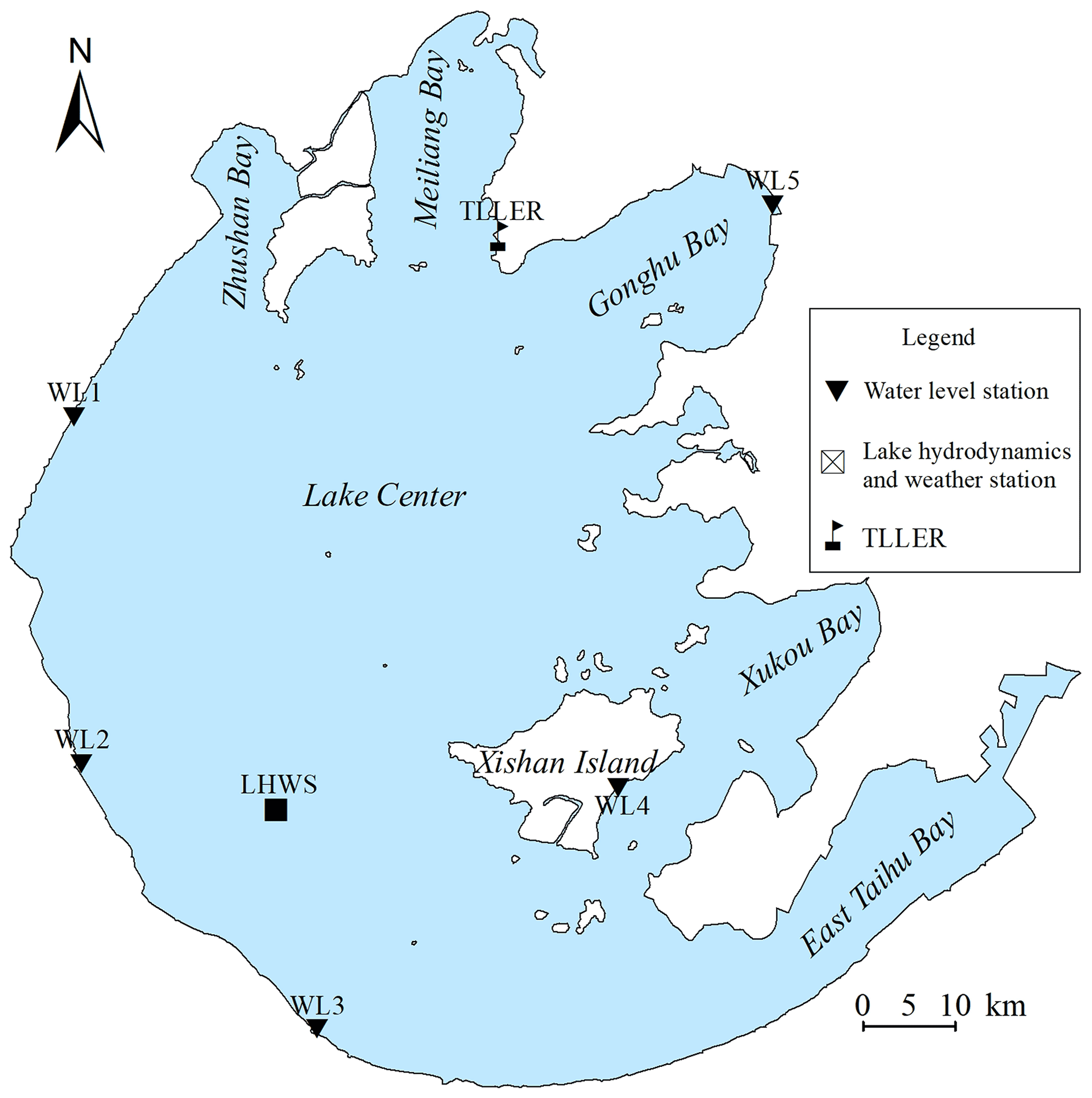
Figure 1Location of the Taihu Laboratory for Lake Ecosystem Research (TLLER), the five water level stations (WL1–WL5), and the lake hydrodynamics and weather station (LHWS) for recording the lake currents and meteorological data.
2.2 Process-based field observations
Two process-based field observations were made in Lake Taihu in summer 2015 (from 00:00 LT on 1 August to 00:00 LT on 12 August 2015) and winter 2018 (from 00:00 LT on 19 December to 00:00 LT on 31 December 2018). Five water level stations (WL1–WL5; Fig. 1) around Lake Taihu built by the Ministry of Water Resources of the People's Republic of China recorded the water level at 60 min intervals. Hourly solar radiation and cloud cover data were also collected from the station of Taihu Laboratory for Lake Ecosystem Research (TLLER).
A lake hydrodynamics and weather station (LHWS) has been established in the area (Fig. 1). At the LHWS, a surface plate equipped with an upward-looking acoustic Doppler profiler (ADP; SonTek Inc., USA; accuracy ±1 % of measured velocity) was fixed on the lake bed. The upward-looking 3000 kHz ADP burst sampled current profiles every 30 min at 1 Hz. Each current profile is divided into 30 total 0.15 m thick current layers. The blanking region height and mounting height of the ADP is 0.7, which implies that no measurements were made within a height of 0.7 m above the lake bed. After the field observations, the effectiveness of the measured current velocity of each current layer is evaluated using the signal-to-noise ratio and water depth recorded by the ADP. The measured effective current velocity of the surface, middle, or bottom current layer is then used to validate the performance of the hydrodynamic models at the same or approximate height.
In addition to the ADP, a portable weather station (WXT520; Vaisala Inc., Finland) was installed 5 m above the lake surface at the LHWS to record the air pressure, wind speed and direction, air temperature, and relative humidity at 10 min intervals. The measured wind speed 5 m above the water surface was adjusted to 10 m (Wu et al., 2018) using the method suggested by the Coastal Engineering Research Center (1984). The water temperature was recorded 1 m below the lake surface at the LHWS using a YSI Sonde 6600 multiparameter water quality sonde (YSI Inc., USA) with an accuracy of ±0.1 ∘C. The wind waves were recorded using an 8 Hz wave recorder (MIDAS; Valeport Ltd., U.K.) during the 2018 field observation.
Many efforts have been made on coupled current–wave model development, especially on the coupling of the Simulating WAves Nearshore model (SWAN; Booij and Holthuijsen, 1999) with existing three-dimensional current models (Chen et al., 2018; Liu et al., 2011; Warner et al., 2008; Wu et al., 2011). However, due to the difficulty in modifying existing model codes (Chen et al., 2018), most coupling models have been developed using third-party software (e.g., Model Coupling Toolkit) rather than by directly merging the original codes. However, this is not yet an efficient way of modifying the descriptions of some key variables in these models. Herein, a Wave and Current Coupled Model (WCCM) is developed by merging the codes of a three-dimensional lake current model (LCM) and SWAN.
3.1 Three-dimensional lake current model
Although most current models largely use same governing equations and solution methods, differences in the programming languages, operating environment, mesh, and description of key processes or parameters impede a full understanding of these models that would allow further code modification. It is thus preferable to develop a new model for determining a suitable description of wind stress, wind waves, and turbulence. The LCM model with a concise and efficient programming is therefore developed to simulate water temperature, water level, and lake currents based on the classic method (Blumberg and Mellor, 1987).
3.1.1 Governing equations
The governing equations of the LCM in the Cartesian coordinate system (Fig. 2) consist of the continuity equation, momentum equations, temperature equation, and density equation (Koue et al., 2018). The sigma (σ) coordinate system is introduced in the vertical direction to eliminate the influence of lake bed topography on the lake current simulations (Fig. 2).

Figure 2Lake bed elevation (h), water level (ζ), and water depth (H) in the Cartesian coordinate system (a). The three components of lake current velocity in the ith (x direction), jth (y direction), and kth (σ direction) grid of the mesh in the sigma (σ) coordinate system (b).
Based on the derivation rule of a composite function, these equations in the Cartesian coordinate system (x′, y′, z, t′) are transformed into the σ coordinate system (x, y, σ, t) using Eqs. (A1.1) through (A1.5).
where u, v, and w are the components of the current velocity in the x, y, and σdirections (m s−1, m s−1, s−1), respectively; h, ζ, and H are the lake bed elevation, water level, and water depth (m), respectively; f is the Coriolis force (s−1) defined by f=2ωsinφ, where ω is the rotational angular velocity of the Earth and φ is the geographic latitude; Fx and Fy are the wave-induced radiation stress in the x and y directions, respectively; ρ and ρ0 are the water and reference density (kg m−3), respectively; g is the gravitational acceleration; AH and AV are the horizontal and vertical eddy viscosity (m2 s−1), respectively; T is the water temperature (∘C); KH and KV are horizontal and vertical turbulent diffusivity (m2 s−1), respectively; Sh and Cp are the heat source term and heat capacity, (J m3 s−1, 4179.98 J kg−1 ∘C−1), respectively; and εU, εV, and εT are the secondary terms introduced by the coordinate system transformation (Eqs. A2.1 through A2.3).
The key parameters and solutions of the continuity equation and momentum equations are demonstrated below, whereas the development and validation of the temperature and density simulations of the LCM will be reported in a separate paper.
3.1.2 Turbulence scheme
To improve the calculation efficiency, the value of the vertical eddy viscosity (AV) is estimated using the Prandtl length l and Richardson number (Ri).
l and Ri are given by
where κ is the von Kármán constant, z0 is the roughness height of the lake bed, and rS is the roughness height of the lake surface.
3.1.3 Boundary conditions
Wind stress at the lake surface is calculated using the following equation:
where ρa is the air density, uw and vw are the wind speed components in the x and y directions 10 m above the lake surface (m s−1), respectively, and Cs is the wind drag coefficient.
The expression of Cs for light winds differs from that for high winds, and a piecewise function is recommended to fit the changes of Cs with wind speed (Large and Pond, 1981). A constant (Cc) is often used to represent Cs below the critical wind speed (Wcr), while a proportional function is adopted for the increase of Cs with wind speed over Wcr. However, referring to Geernaert et al. (1987), Cs approaches a constant of ∼0.003 for wind speeds higher than 20 m s−1. We therefore propose that a logistic function is more reasonable to derive the expression of Cs under high-wind conditions. The wind components in the x and y directions are used to calculate Cs in the x and y directions, respectively. The x-direction component is calculated using the following equation:
The y direction component is calculated using the following equation:
In the above equations, f(uw) and f(vw) are the logistic functions.
Friction at the lake bed is calculated using the following equation:
where CB is the bottom friction coefficient given by
3.1.4 Wave-induced radiation stress
Wave–current interaction is a complicated process (Mellor, 2008) and remains poorly understood. Longuet-Higgins and Stewart (1964) first proposed the concept of wave-induced radiation stress, and Sun et al. (2006) derived the following expressions of the stress for three-dimensional current numerical models:
where HS is the significant wave height (m), T0 is the wave period (s), L is the wavelength (m), θm is the mean wave direction, and θ1 is the angle between the mean wave direction and geographical east direction.
3.1.5 Solution of equations
The splitting mode technique (Blumberg and Mellor, 1987) and alternation direction implicit difference scheme (Butler, 1980) are used to discretize Eqs. (1)–(3) on the staggered grid (Figs. 2, 3). A detailed description of the solution of equations is provided in Appendix A3.

Figure 3Structure of the Wave–Current Coupled Model (WCCM) obtained by two-way coupling SWAN and LCM models, with the variable definitions and the data transmission between the meshes.
3.2 Simulating WAves Nearshore model
In view of the importance of wind waves in the hydrodynamic and ecological processes of shallow lakes, the SWAN model has been frequently used to simulate wind waves in Lake Taihu (Wang et al., 2016; Wu et al., 2019; Xu et al., 2013). The governing equation for the SWAN is the following wave action balance equation:
where N is the action density spectrum; t, x, and y are the time and horizontal coordinate directions, respectively; σ1 is the relative frequency; θ is the wave direction; cx, cy, , and cθ denote the wave propagation velocity in x, y, σ1, and θ space, respectively; and S is the source in terms of energy density, which represents the effects of generation, dissipation, and nonlinear wave–wave interactions. HS, T0, L, and θm are deduced from the value of N(x, y, t, σ1, θ) (Booij et al., 2004).
The action balance equation is solved in the Cartesian coordinate system using a first-order upwind scheme of the finite-difference method (Booij et al., 1999, 2004).
3.3 Two-way coupling of the LCM with SWAN
The SWAN and LCM were coupled to establish the WCCM model (Fig. 3). The current speeds u and v and water level ζ computed by the LCM model are inputs for the SWAN model. The HS, T0, L, and θm values computed using the SWAN model are used as inputs in the LCM model to compute the wave-induced radiation stresses Fx and Fy (Eqs. 15, 16).
3.4 Configuration of the WCCM in Lake Taihu
The WCCM is used to simulate wind waves and lake currents in Lake Taihu during the process-based field observation periods. Referring to existing model studies in Lake Taihu (Hu et al., 2006; Mao et al., 2008; Liu et al., 2018), the horizontal computation domain of Lake Taihu (Fig. 1) for the LCM is divided into cells with a 1 km resolution to improve the computing efficiency. The water column is divided into five layers in the vertical direction, the time step is 30 s, and the α value is 0.5.
Lake Taihu is considered a closed lake for the simulation because the influence of inflows and outflows on the current field is very small compared with the influence of wind stress (Li et al., 2011; Wu et al., 2018; Zhao et al., 2012). The simulations therefore disregard the inflows and outflows. The model inputs at the air–water boundary include air temperature, surface air pressure, cloud cover, relative humidity, and wind speed and direction collected from the LHWS and TLLER (Fig. 1). The initial condition for the water level was determined via interpolating the water level values measured at stations WL1–WL5 at the beginning of the model integration. The initial water temperature was set to the measured values recorded by the ADP and YSI Sonde at the beginning of the model integration, and the current speed was initialized to 0 m s−1.
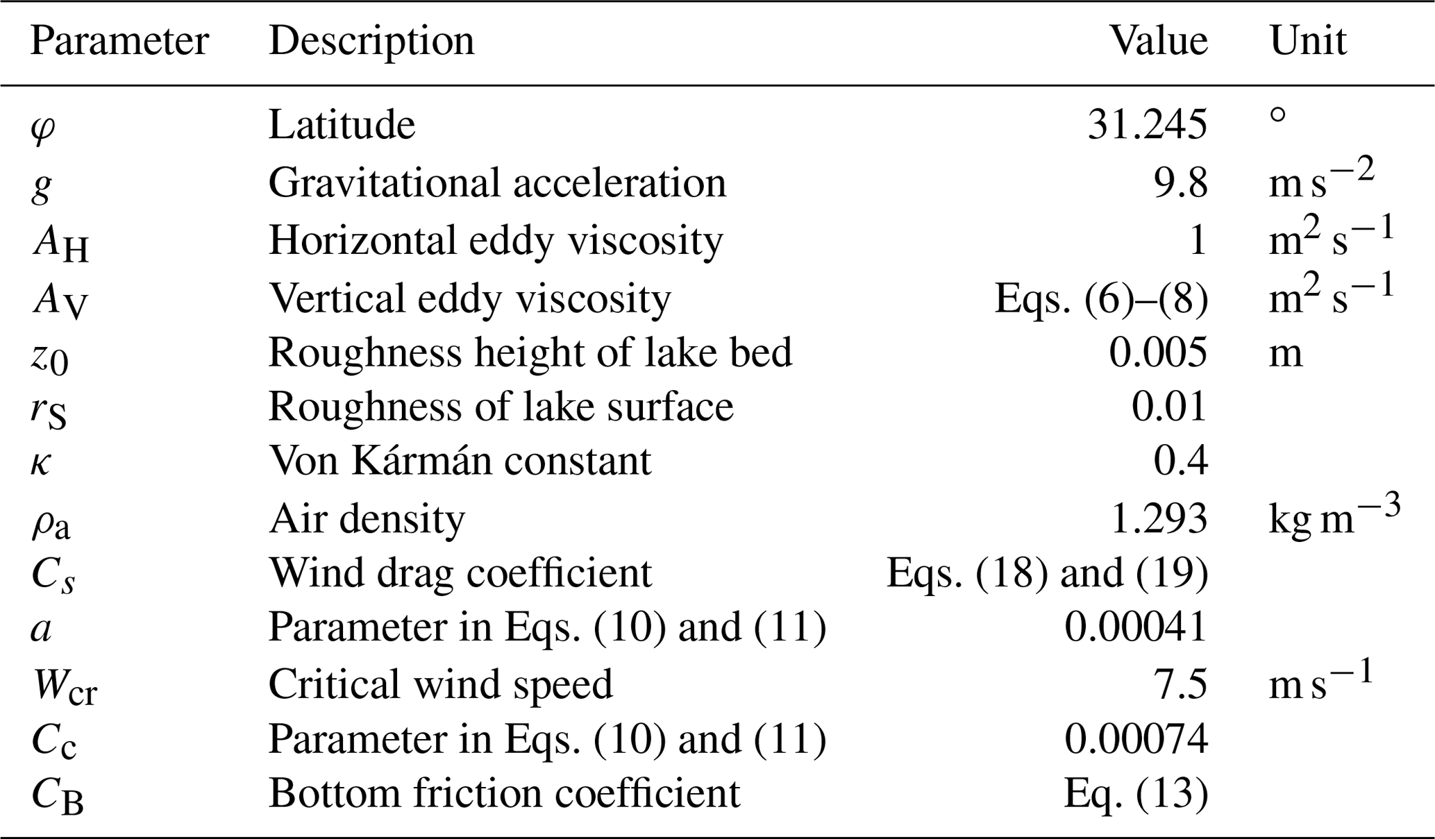
A total of 10 parameters must be determined for the LCM simulation (Table 1). Among them, φ, g, κ, and ρa are constants, while the AV and CB values can be calculated from the κ, z0, and rS values. AH and z0 values are the same as those used for the EFDC, and rS is set to 0.01 (Table 1).
Table 1Parameter values and variable equations used for lake current simulation in the LCM.
The parameters in Eqs. (10) and (11) are determined as follows. A critical wind speed of 7.5 m s−1 is used to distinguish between light and high winds as it is equal to the wind speed for defining an aerodynamically rough water surface (Wu, 1980). The expression of the logistic function in Eq. (10) or (11) is preliminarily determined under high-wind conditions referring to the curve of Edson et al. (2013) (Fig. 4) and an upper Cs limit of ∼0.003 (wind speed >20 m s−1; Geernaert et al., 1987), The process-based observation data from 2015 are then used to determine the logistic expression and parameters of a and Cc by the trial and error method. This is done for the x direction using the following equation.
This is done for the y direction using the following equation.
The SWAN model mesh is the same as the LCM horizontal mesh. Considering their randomness, the characteristic wind wave values are typically represented by the statistical values of the high-frequency pressure records over a 10 min period. The time increment of the SWAN model was therefore set to 600 s. The frequency band was set to 0.04–4 Hz and the wave direction ranged from 0 to 360∘ with an increment of 6∘. The second-generation mode was used to calculate the source term (e.g., wind input, depth-induced wave breaking, bottom friction, triads). The parameter cdrag of the SWAN model was set to 0.00133, and the Collins bottom friction coefficient was set to 0.025. The calibration and validation of these parameters have been reported in previous studies (Xu et al., 2013; Wang et al., 2016). Our study also verifies that the SWAN in the WCCM can accurately simulate the change in significant wave height at LHWS during the 2018 field observations (Fig. B.1).
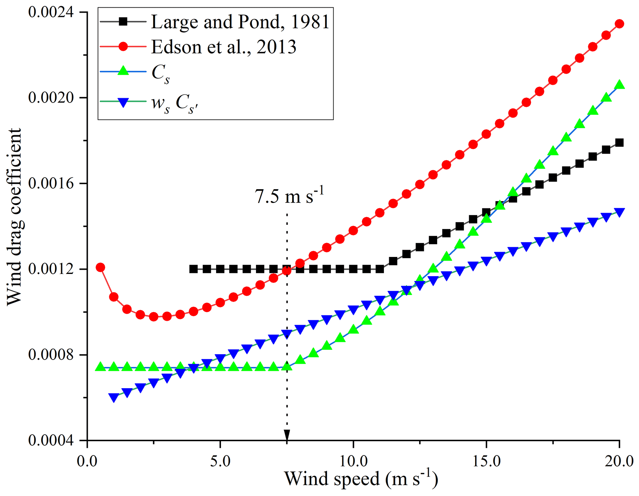
Figure 4Changes in wind drag coefficient with wind speed calculated by the equations proposed by Large and Pond (1981), Edson et al. (2013), Cs and wsCs′.
Considering the time of the wind peaks and the cold start of the WCCM, the hydrodynamics time series of the latter half of the 2015 summer observation (from 00:00 LT on 8 August to 00:00 LT on 12 August 2015) were used to calibrate the WCCM, and those of the latter half of the 2018 winter observation (from 00:00 LT on 26 December to 00:00 LT on 31 December 2018) were used to evaluate the WCCM performance.
The WCCM can be used to simulate the changes of water temperature in Lake Taihu (Fig. B.2), which will be discussed in detail in a separate paper. Here, only the WCCM simulations of the lake currents are evaluated.
3.5 Methods
3.5.1 Statistical analysis
To evaluate the WCCM performance, the mean absolute error (MAE), root-mean-square error (RMSE), and correlation coefficient (r) between the measured and simulated values at both significance levels of p<0.05 and p<0.01 are reported. The magnitude of the lake current speed is expressed as the mean ± standard deviation.
The mean absolute error of the horizontal current direction (MAEUVD) is used to compare the simulated and measured values:
ArcGIS 10.2 (ESRI Inc., USA) was used to process the spatial data, and Tecplot 360 (Tecplot Inc., USA) was used to draw the contours of the water level, current field, and stream traces.
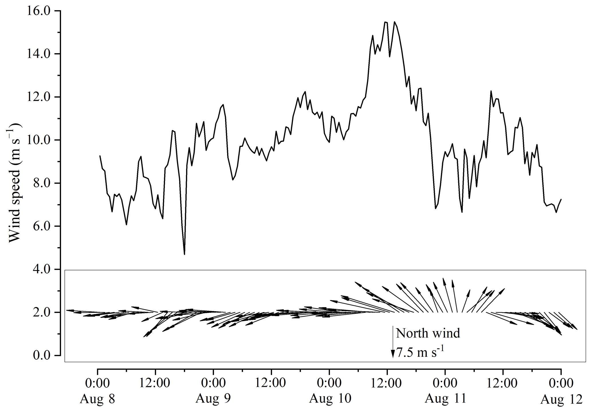
Figure 5Variation of wind speed and wind direction at 10 m above the water surface at the LHWS during the 2015 summer observation.
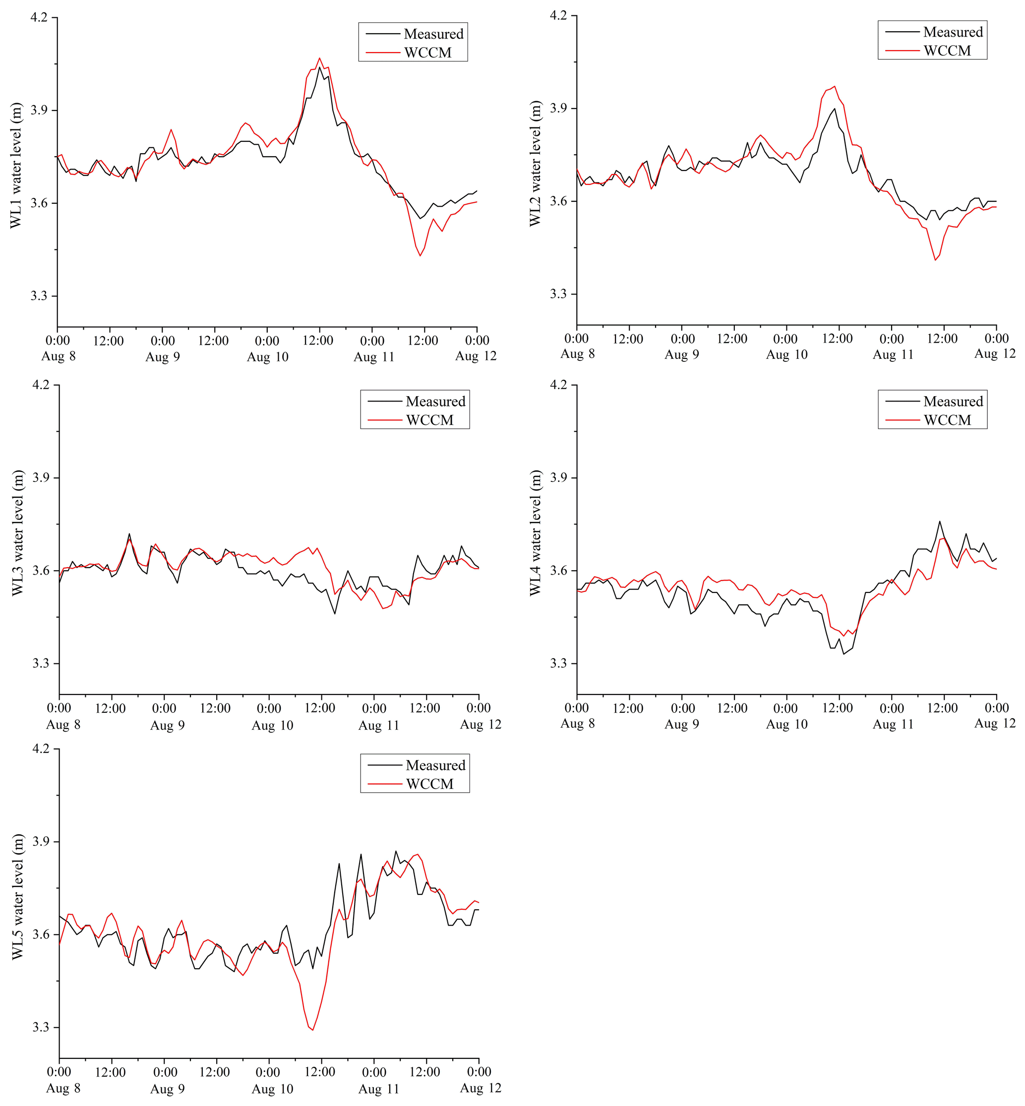
Figure 6Comparison between the WCCM-simulated and measured water levels at the WL1–WL5 stations during the 2015 summer observation.
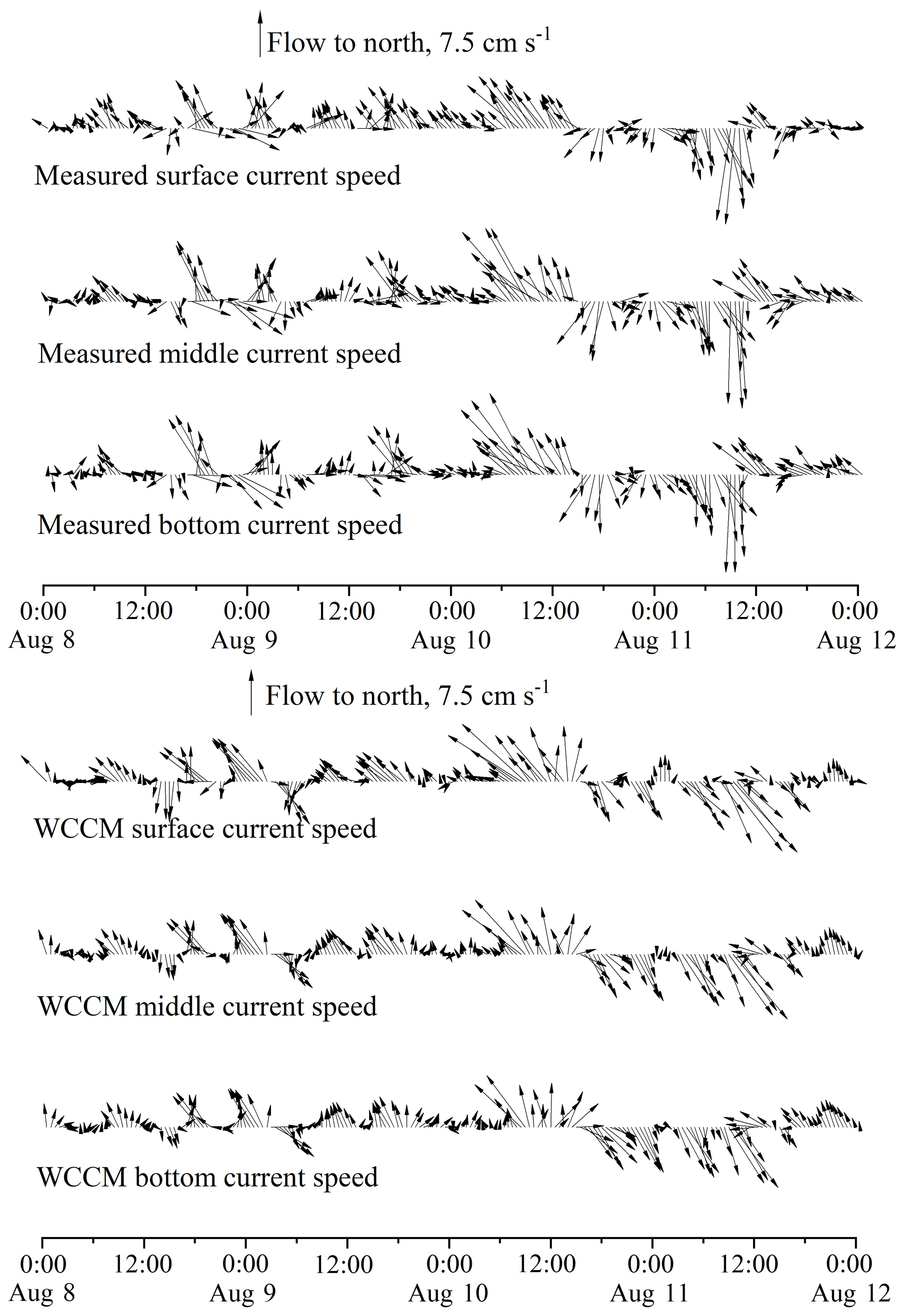
Figure 7Comparison between the measured and WCCM-simulated current speeds in the lake surface, middle, and bottom water layers at the LHWS during the 2015 summer observation.
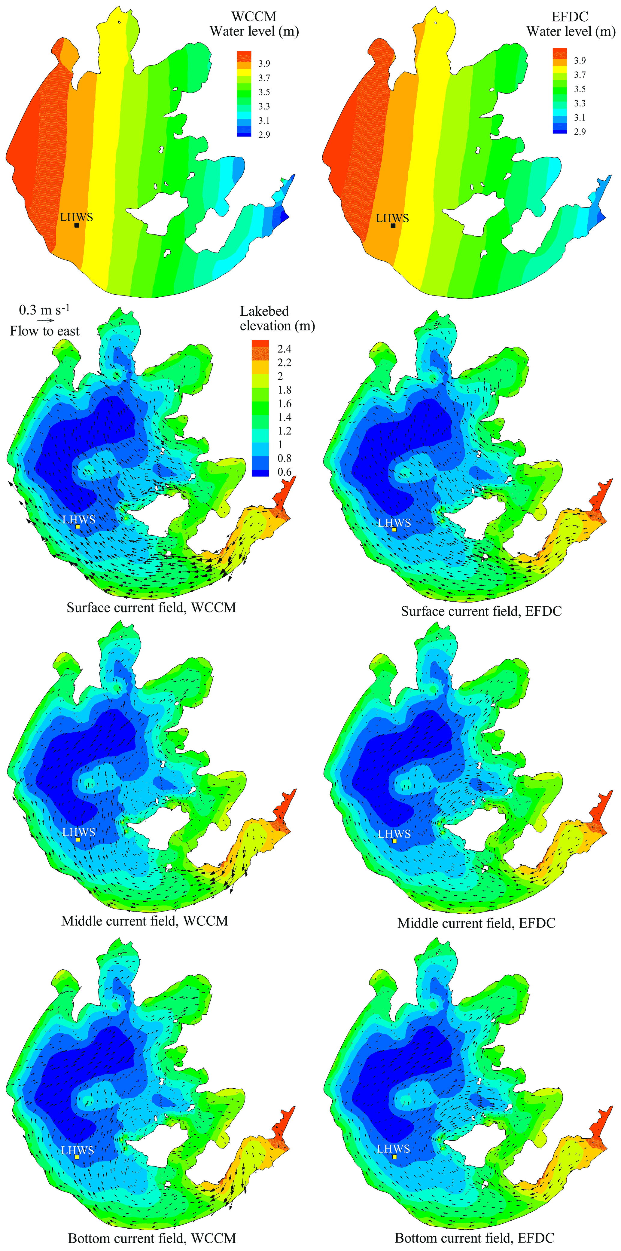
Figure 8Comparison of the contour of water level and current fields in the surface, middle, and bottom water layers simulated by the WCCM with those simulated by the EFDC at 13:00 LT on 10 August 2015.
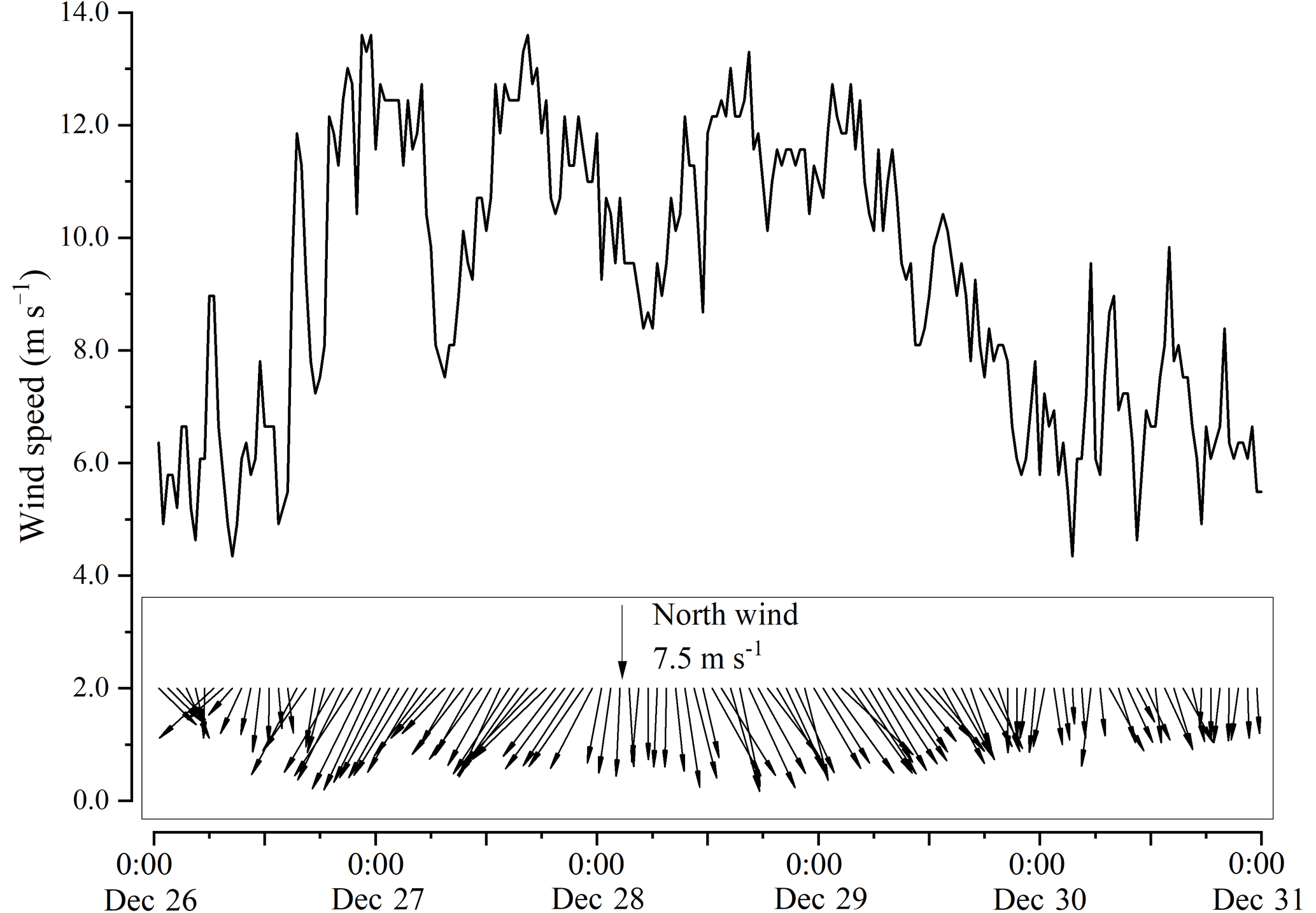
Figure 9Variation of wind speed and direction at 10 m above the water surface at the LHWS during the 2018 winter observation.
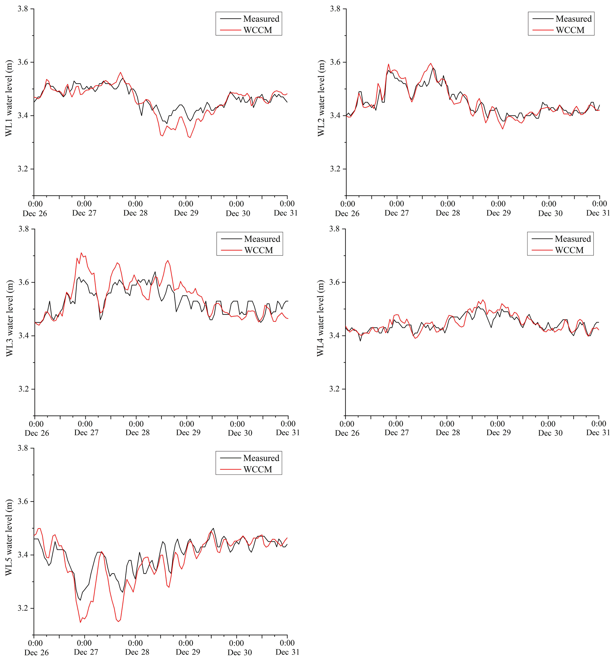
Figure 10Comparison between the WCCM-simulated and measured water levels at the WL1–WL5 stations during the 2018 winter observation.
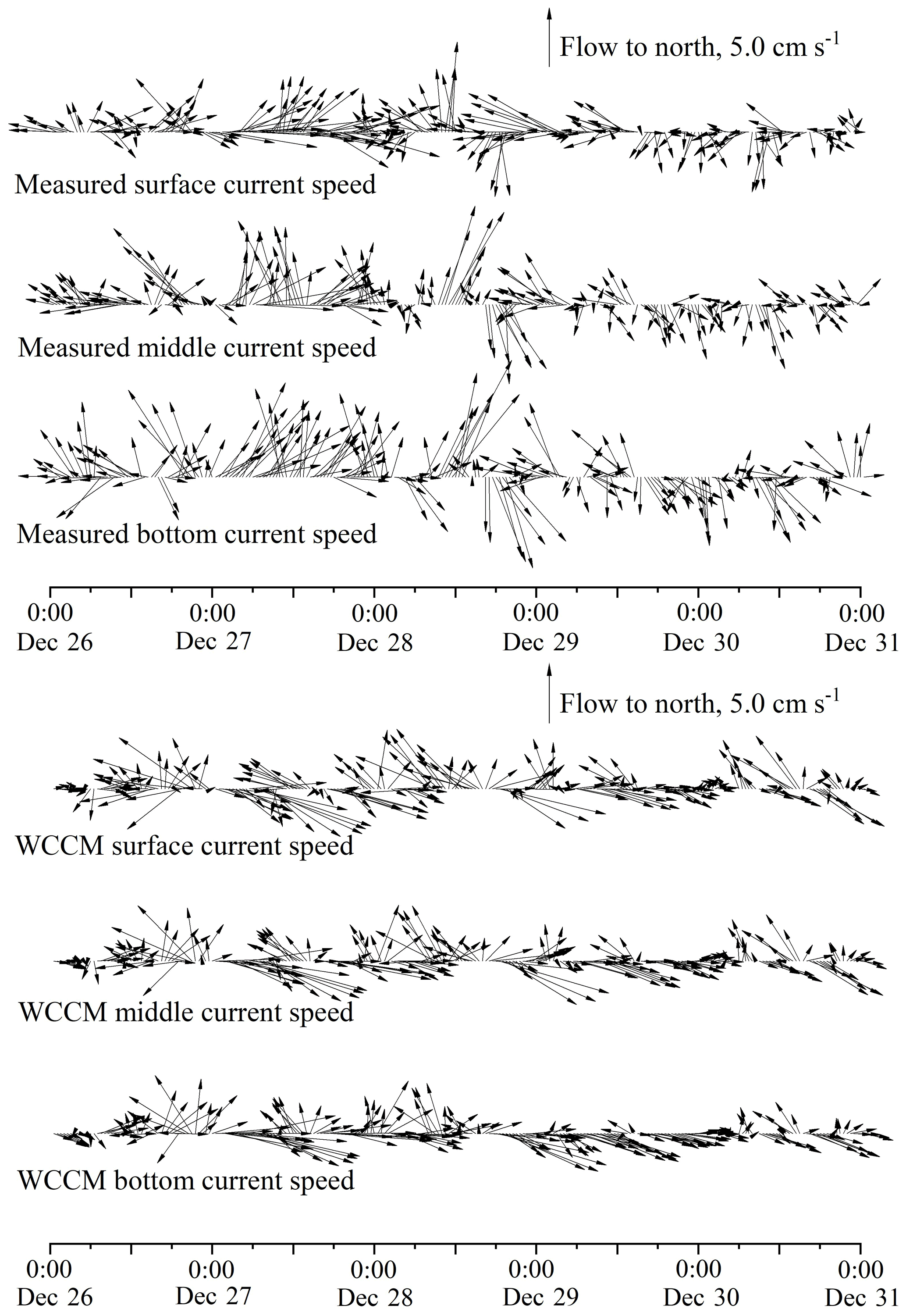
Figure 11Comparison between the measured and WCCM-simulated surface, middle, and bottom current speeds at the LHWS during the 2018 winter observation.
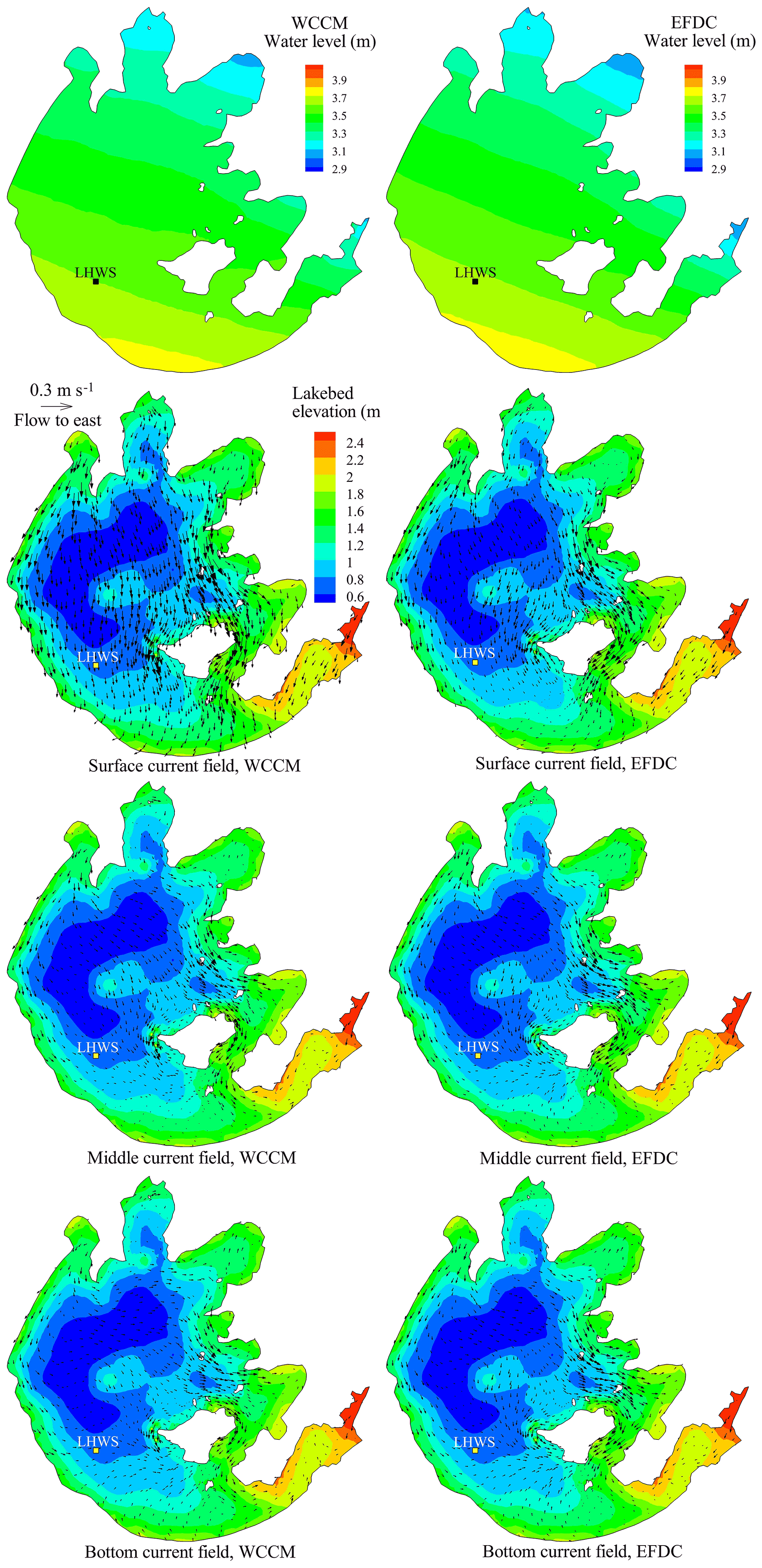
Figure 12Comparison of the contour of the water level and surface, middle, and bottom current fields simulated by the WCCM with those simulated by the EFDC at 22:00 LT on 26 December 2018.
3.5.2 Comparison between the WCCM and EFDC
A comparison between different models is a useful method to study currents in large water bodies (Huang et al., 2010; Morey et al., 2020; Soulignac et al., 2017). The EFDC is one of the most widely used models for shallow lakes worldwide (Chen et al., 2020) and offers a general-purpose modeling package to simulate three-dimensional flow, transport, and biogeochemical processes in surface water systems (Ji et al., 2001; Ji, 2008). The EFDC has been successfully applied in Lake Taihu (Li et al., 2011; 2015; Wang et al., 2013). Here, the EFDC is used to evaluate the WCCM performance.
The EFDC hydrodynamic model was developed by Hamrick (1992), and its governing equations are the same as Eqs. (1)–(3). It uses the splitting mode technique to solve the continuity equation and momentum equation in the σ coordinate system. The Mellor–Yamada turbulence model is used in the EFDC to calculate the vertical eddy viscosity (Ji et al., 2001). The wind stress in the EFDC is calculated using the following equations (Hamrick, 1992; Li et al., 2015; Wu et al., 1980):
where and ws are wind drag coefficient and wind shelter coefficient in the EFDC, respectively (Fig. 4).
The mesh used for the EFDC simulation is the same as that in the LCM and WCCM. After consulting with the authors of the uncertainty and sensitivity analysis performed on the hydrodynamic parameters of the EFDC for Lake Taihu (Li et al., 2015), the optimal horizontal eddy viscosity was set to 1 m2 s−1, the roughness height was set to 0.005 m, and ws was set to 0.7.
3.5.3 Numerical experiments
Four numerical experiments were designed to evaluate the accuracy of the WCCM and identify the relative importance of wind stress, wind waves, and turbulence in improving the simulation of the wind-driven currents.
-
Experiment 1 (EFDC) is a numerical simulation of the lake currents using the EFDC. The Mellor–Yamada turbulence scheme is used and the drag coefficient is given by Eqs. (22) and (23), but the wave-induced radiation stress is not considered (no coupling with SWAN).
-
Experiment 2 (LCM_1) is numerical simulation of the lake currents using the LCM with the same drag coefficient expression as in EFDC (Eqs. 22 and 23) but using a different turbulence scheme, as given in Eqs. (6)–(8), and without considering wave-induced radiation stress.
-
Experiment 3 (LCM_2) is the same experiment as LCM_1 with a different expression of the drag coefficient, as given in Eqs. (18) and (19), and without considering wave-induced radiation stress.
-
Experiment 4 (WCCM) is the same experiment as LCM_2 but considering wave-induced radiation stress to achieve the two-way coupling model.
4.1 Summer observation and model calibration in 2015
The average wind speed over Lake Taihu between 00:00 LT on 8 August and 00:00 LT on 12 August, 2015 was 9.9 m s−1 (Fig. 5), with a maximum of 15.5 m s−1 at 13:00 LT on 10 August, corresponding to a wind direction of 107.5∘. Lake Taihu experienced a strong east–southeast wind event during the 2015 summer observation.
Table 2Correlation coefficient (r) and root-mean-square error (RMSE) between the simulated and measured water level during 2015 summer observation for the numerical experiments. Note that * indicates p<0.05 and that ** indicates p<0.01.

The mean water level observed at the five stations was 3.64±0.01 m, with a maximum of 4.04 m recorded at the WL1 station at 12:00 LT on 10 August (Fig. 6), corresponding to 3.38 m recorded at the WL4 station. The average r values between the simulated and measured water levels of the EFDC, LCM_1, LCM_2, and WCCM are 0.87, 0.88, 0.86, and 0.86 (p<0.01; Table 2), respectively, and the average RMSE values are 0.05, 0.05, 0.05, and 0.04 m, respectively.
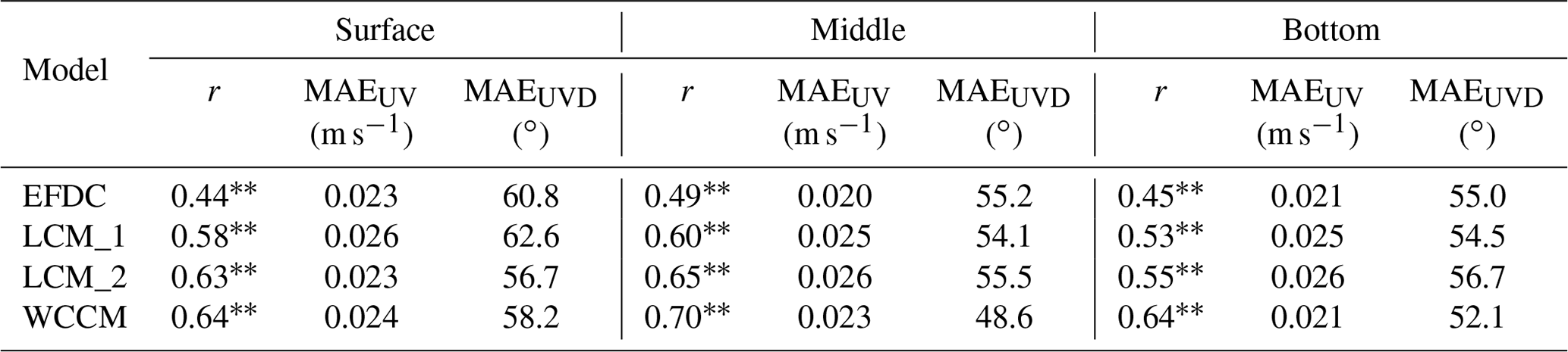
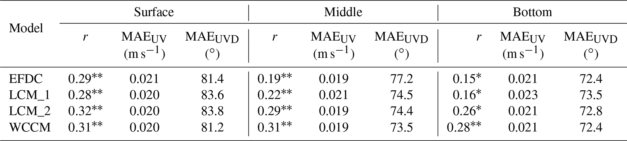
The mean measured surface, middle, and bottom current speeds at the LHWS (Fig. 7) were 5.0±3.0, 5.5±3.5, and 5.4±3.6 cm s−1, respectively. The average r values between the simulated and measured current speeds of EFDC, LCM_1, LCM_2, and WCCM are 0.46, 0.57, 0.61, and 0.66 (p<0.01; Table 3), respectively, while the average MAEUVD values are 57, 57.1, 56.3, and 52.9∘, respectively.
Table 3Correlation coefficient (r) and mean absolute error between the simulated and measured current velocity (current speed, MAEUV; current direction, MAEUVD) during the 2015 summer observation for the numerical experiments. Note that * indicates p<0.05 and that ** indicates p<0.01.
The contours of the water level simulated by the WCCM at 13:00 LT on 10 August, corresponding to the time of the maximum wind speed, are similar to those of the EFDC simulation and show a decreasing trend from northwest to southeast (Fig. 8). The surface current field simulated by these two models mainly flows from southeast to northwest, which is further demonstrated by the simultaneous stream traces (Fig. B3). The middle and bottom current fields of the southern part of the lake are consistent with the surface current field, but those in the center and northern parts of the lake mainly flow from southwest to northeast.
A major difference between the WCCM- and EFDC-simulated current fields is the significantly higher current speed simulated by the former (Fig. 8). There are vortexes produced by the WCCM in the upwind area, such as in Xukou Bay and northwest of Xishan Island (Fig. B.3). In contrast, the vortexes simulated by the EFDC tend to be located in the downwind area, such as Zhushan Bay and Meiliang Bay.
4.2 Winter observation and model validation in 2018
The average wind speed over Lake Taihu is 9.2 m s−1 between 00:00 LT on 26 December and 00:00 LT on 31 December 2018 (Fig. 9) with a maximum of 13.6 m s−1 at 22:00 LT on 26 December, corresponding to a wind direction of 26.3∘. Lake Taihu experienced a strong north–northeast wind event during the 2018 winter observation.
The mean water level over the five stations was 3.46±0.01 m with a minimum of 3.23 m recorded at the WL5 station at 22:00 on 26 December, corresponding to a secondary peak of 3.62 m recorded at the WL3 station (Fig. 10). The EFDC, LCM_1, LCM_2, and WCCM-simulated water levels at each water level station significantly correlate with the measured values (p<0.01; Table 4). The average r values are 0.87, 0.88, 0.88, and 0.87, respectively, and the average RMSE values are 0.04, 0.05, 0.03, and 0.03 m, respectively.
Table 4Correlation coefficient (r) and root-mean-square error (RMSE) between the simulated and measured water level during the 2018 winter observation for the numerical experiments. Note that * indicates p<0.05 and that ** indicates p<0.01.

The mean measured surface, middle, and bottom current speeds at the LHWS (Fig. 11) were 3.7±2.0, 3.5±2.0, and 4.2±2.2 cm s−1, respectively. The average r values of the simulated and measured current speed of the EFDC, LCM_1, LCM_2, and WCCM are 0.21, 0.22, 0.29, and 0.3 (p<0.05; Table 5) respectively, while the average MAEUVD values are 77, 77.2, 77, and 75.7∘, respectively.
Table 5Correlation coefficient (r) and mean absolute error between the simulated and measured current velocity (current speed, MAEUV; current direction, MAEUVD) during the 2018 winter observation for the numerical experiments. Note that * indicates p<0.05 and that ** indicates p<0.01.
The water level contours simulated by the WCCM at 22:00 LT on 26 December 2018, corresponding to the time of the maximum wind speed, are similar to those of the EFDC and show a deceasing trend from southwest to northeast (Fig. 12). The surface current fields simulated by these two models mainly flow from north to south, which can be further demonstrated by the simultaneous stream traces (Fig. B4). The middle and bottom current fields mainly flow from northwest to southeast.
The main difference between the WCCM- and EFDC-simulated current fields is that the current speed simulated by the former is significantly higher (Fig. 12). Clockwise vortexes form in Gonghu Bay in the surface, middle, and bottom current fields simulated by the EFDC (Fig. B.4), whereas this clockwise vortex is only located in the middle current field simulated by the WCCM.
Influenced by the strong east–southeast wind event during the 2015 summer observation, a maximum water level difference of 0.66 m occurred at 12:00 LT on 10 August between WL1 in the downwind lake area and WL4 station in the upwind lake area (Fig. 6). Prior to this maximum, all of the measured surface, middle, and bottom currents flowed along the wind direction and their speed significantly increased (Fig. 7). The strong east–southeast winds drive the entire water column at the LHWS to form wind-driven currents, thus resulting in a downwind upwelling (Wu et al., 2018). Similarly, generated by the strong north–northeast wind event during the 2018 winter observation, wind-driven currents also resulted in downwind upwelling (Fig. 11). These upwelling processes provided an excellent opportunity to evaluate the performance of the WCCM in Lake Taihu.
The numerical solutions of the governing equations and most parameter values of the WCCM are similar to those of the EFDC. The main differences between the two models are the vertical eddy viscosity, wind drag coefficient, and wave-induced radiation stress. The numerical experiments show that the average correlation coefficient between the WCCM-simulated and measured current speeds increased by 36.4 % compared to the LCM_1 results or 42.9 % compared to the EFDC results in 2018. The current direction and field simulated by the WCCM also improved, whereas the water level was simulated at a similar accuracy to that of the EFDC. Compared with the reference model, the WCCM is more reliable to simulate wind-driven currents and subsequent downwind upwelling in Lake Taihu. The WCCM can also accurately simulate wind waves and water temperature in the lake (Figs. B1 and B2).
5.1 Wind drag coefficient
The wind drag coefficient is a key parameter for hydrodynamic numerical models. The EFDC parameter sensitivity analysis shows that the wind drag coefficient is the most sensitive parameter for simulating the current velocity in Lake Taihu (Li et al., 2015). Our numerical experiments also indicate that the correlation coefficients between the simulated and measured current speeds of LCM_2 and WCCM are significantly greater than those of EFDC and LCM_1 (Tables 3, 5). This implies that the new expressions of Cs (Eqs. 18 and 19) mainly contribute to the enhanced correlation coefficients. Based on previous studies (Edson et al., 2013; Geernaert et al., 1987; Large and Pond, 1981; Xiao et al., 2013) and our field observations, these expressions were derived to describe the discontinuity of changing trend of Cs with wind and directionality of the wind momentum transmission.
The magnitude of Cs represents the transmission efficiency of the wind momentum to a waterbody, and its change is discontinuous. Surface waves can increase the roughness of a lake surface and further influence the transmission efficiency (Xiao et al., 2013). The transmission efficiency on aerodynamically rough water surfaces is higher than that on aerodynamically smooth water surfaces (Lükő et al., 2020). Wu (1980) proposed that the atmospheric surface layer appears to be aerodynamically rough when the wind speed exceeds 7.5 m s−1. This implies that there is a discontinuity of the Cs curves at wind speeds of 7.5 m s−1. Field observations in Lake Taihu (Xiao et al., 2013) indicate that the measured Cs initially decreased under light-wind conditions (<∼7.5 m s−1) and then increased under high-wind conditions (>∼7.5 m s−1). The curves of Cs plotted by the equation proposed by Edson et al. (2013) and Large and Pond (1981) also intersect at a wind speed of 7.5 m s−1 (Fig. 4). A wind speed of 7.5 m s−1 is therefore reasonable for defining the discontinuity of changing trend of Cs with wind in Lake Taihu.
As shown in Eqs. (18) and (19), a logistic curve is used to describe the increase of Cs for wind speeds >7.5 m s−1; otherwise Cs is a constant. Under light-wind conditions, the mechanism of the Cs change with wind speed remains incompletely understood and its mathematic description is non-deterministic (Fig. 4). According to a tremendous amount of measured Cs values reported by Edson et al. (2013), the points between Cs and wind speed evenly distribute on both sides of a constant under light-wind conditions. A constant is therefore suitable (Large and Pond, 1981). Under high-wind conditions, the proportional function is most frequently used to fit the Cs change (Geernaert et al., 1987; Large and Pond, 1981; Wu, 1980; Zhou et al., 2009). However, the measured Cs values indicate more rapid changes than described by the proportional function (Edson et al., 2013). Furthermore, Geernaert et al. (1987) concluded that Cs increases to a constant (∼0.003) by compiling all of the reported Cs measurements. The logistic function is therefore used to fit the rapid increase that then tends toward a constant. It should also be noted that the curves of Eqs. (18) and (19) and ws× Eq. (23) used in this study are significantly lower than the other two curves (Fig. 4). The main cause is that the limited water depth and fetch in Lake Taihu reduce the transmission efficiency of the wind momentum and restrict the development of wind-driven currents in the lake.
The directionality of wind momentum transmission is further addressed using different Cs values in the x and y directions. There have been numerous expressions designed to calculate the wind drag coefficient based on ocean environments without consideration of the directionality of wind momentum transmission (Geernaert et al., 1987; Large and Pond, 1981; Lükő et al., 2020; Wu, 1980; Zhou et al., 2009). However, the increase of transmission efficiency with wind speed (Lükő et al., 2020) will result in a contradiction in these existing expressions, i.e., that the same Cs values are used in x and y direction while the components of wind speed in these directions are different. Moreover, wind waves and lake seiche also have directionality, which can affect the transmission efficiency of the wind momentum by changing the roughness and tilt of the lake surface. Neglecting the directionality of wind momentum transmission can therefore overestimate or underestimate the wind drag coefficient in any one direction in large shallow lakes.
5.2 Wave-induced radiation stress
Wave-induced radiation stress is first considered in simulating wind-driven currents in large shallow lakes. The results show that this consideration can improve the simulated current direction. The MAEUVD values of the LCM_2 (average MAEUVD of 56.3∘; Table 3) in 2015 are greater than those of the WCCM (average MAEUVD of 52.9∘; Table 4). A similar result can be achieved by comparing the MAEUVD values between the LCM_2 and WCCM in 2018 (Table 5). Moreover, the correlation coefficients of LCM_2 in 2018 are slightly lower than those of the WCCM in 2018 (Table 5), which implies that wave-induced radiation stress can also contribute to the improvement of the WCCM-simulated current speed.
A comparison between the WCCM- and EFDC-simulated current fields further demonstrates the importance of wave-induced radiation stress. Although the current field simulated by the WCCM is similar to that simulated by the EFDC, the vortex locations simulated by these models are quite different. In 2015, the middle and bottom current fields simulated by the EFDC exhibit counterclockwise vortexes in Zhushan Bay and Meiliang Bay (Fig. B.3), which are located in the downwind area, but the current fields simulated by the WCCM do not show the same phenomenon. This is because the interaction between wind waves and lake currents in the downwind area is turbulent owing to wave deformation resulting from the shallow water and lakeshore. The wave-induced radiation stress therefore reduces the likelihood that a vortex will form in this area. Conversely, the middle and bottom current fields simulated by the LCM_2 without wave-induced radiation stress also show counterclockwise vortexes in Zhushan Bay and Meiliang Bay (Fig. B.5), which is similar to the EFDC result. It is very important for Lake Taihu that the absences of vortexes in the downwind area reinforce the accumulation of buoyant cyanobacteria and further promote cyanobacterial blooms within this area.
5.3 Vertical eddy viscosity
Vertical eddy viscosity plays a less prominent role in the development of wind-driven currents than the other variables. In this study, the Mellor–Yamada level 2.5 turbulence closure model (Mellor and Yamada, 1982; Ji et al., 2001) is adopted in the EFDC, and the other parameters are determined after parametric uncertainty and sensitivity analysis (Li et al., 2015), while a simple turbulence scheme (Eqs. 6–8) is adopted in the LCM_1. However, the accuracy of the LCM_1 is rather similar to that of the EFDC (Tables 2–5), which implies that the high-order turbulence scheme does not improve the lake current simulations (Koue et al., 2018), whereas the simple turbulence scheme makes the WCCM more efficient.
5.4 Challenges of the hydrodynamic model development for shallow lakes
Although the WCCM performance has been improved relative to the reference models of the EFDC, LCM_1, and LCM_2, the correlation between WCCM-simulated and ADP-measured current speed remains low, and the mean of the simulated current speed is lower than that of the measured current speed. Similar conclusions can be drawn from the model validation studies in other lakes (Huang et al., 2010; Jin et al., 2000; Ishikawa et al., 2021; Soulignac et al., 2017). There are three possible explanations for this problem. First, based on the Doppler effect of sound waves, the ADP measures the three-dimensional lake currents by detecting the movement of suspended particle matter (SPM) in water column. However, the spatiotemporal distributions of the concentration and physicochemical properties of the SPM are changeable in lakes (Zheng et al., 2015). This will undoubtedly influence the measurements of real currents in lakes. Second, the spatiotemporal resolution of the numerical model input data can introduce errors into the lake current simulations, including mesh, underwater topography, boundary conditions, and wind field. Third, the wind-induced hydrodynamics in large shallow lakes are not fully understood. For example, Eqs. (18) and (19) derived from the field observations are only effective when the wind speed is ≤15.5 m s−1, which is the maximum of the field observations, meanwhile the contributions of the wind waves to the development of wind-driven currents are underestimated in Lake Taihu.
Strong summer or winter winds generate wind-driven currents in Lake Taihu, which subsequently results in downwind upwelling events. The WCCM has been developed to reconsider the expression of wind stress, wind waves, and turbulence based on these events and numerical experiments. This model can simulate the development of wind-driven currents with a 42.9 % increase of simulated current speed compared with the EFDC results of 2018. The new expression for the wind drag coefficient is mainly responsible for increasing the correlation coefficient between the WCCM-simulated and measured current speeds. The introduction of wave-induced radiation stress can contribute to the improvement of the simulated current direction and fields, and slightly improve the current speed simulation. The simple parameterized turbulence scheme is sufficient for simulating wind-driven currents in Lake Taihu. We emphasize that more process-based field observations using advanced instruments are required to fully understand the real hydrodynamic characteristics of large shallow lakes and further improve the performance of lake hydrodynamic models, especially for the interaction between wind waves and lake currents.
A1 Methods of coordinate transformation
where ψ is u, v, w, and T in the sigma coordinate system and w′ is the vertical velocity in the Cartesian coordinate system, m s−1.
A2 Secondary terms
A3 Solution of equations
Using the splitting mode technique (Blumberg and Mellor, 1987) and alternation direction implicit algorithm (Butler, 1980), the external mode is derived by vertically integrating the momentum equations to solve the change in water surface that feedbacks onto the internal mode and solves the vertical current velocity. Equations (1)–(3) are vertically integrated, and and are used to represent the current speeds in the x and y directions. Equations (1)–(3) can then be transformed as follows:
where BU and BV are shown in Eqs. (A2.4) and (A2.5).
The expressions of the internal mode can be achieved using Eq. (2) minus Eq. (A3.2) and Eq. (3) minus Eq. (A3.3):
where , , and DU and DV are shown in Eqs. (A2.6) and (A2.7).
These equations are discretized using the finite-difference method. For the external mode equations, the alternation direction implicit difference scheme and staggered grid (Figs. 2, 3) are used to discretize Eqs. (A3.1) and (A3.2) and then obtain the equation to calculate U in the next time increment:
where α is the format weight coefficient. When α=1, Eqs. (A3.6) and (A3.7) are explicit (otherwise they are implicit). The definition of each variable on the staggered grid is shown in Figs. 2 and 3.
According to the U value in next time increment, ζ and V can be calculated by
Similarly, the alternation direction implicit difference scheme is used to discretize Eqs. (A3.4) and (A3.5) of the internal mode to obtain
The chasing algorithm is used to solve the tridiagonal matrix formed by Eqs. (A3.10) and (A3.11). The current numerical model was built based on these governing equations and written in Intel Visual Fortran (Intel Inc. USA).
Figure B1Correlation coefficient (r) and mean absolute error (RMSE) between measured and WCCM-simulated significant wave height at the LHWS during the 2018 field observation.

Figure B2Correlation coefficient (r) and mean absolute error (RMSE) between measured and WCCM-simulated water temperature at the LHWS during the 2015 and 2018 field observations.
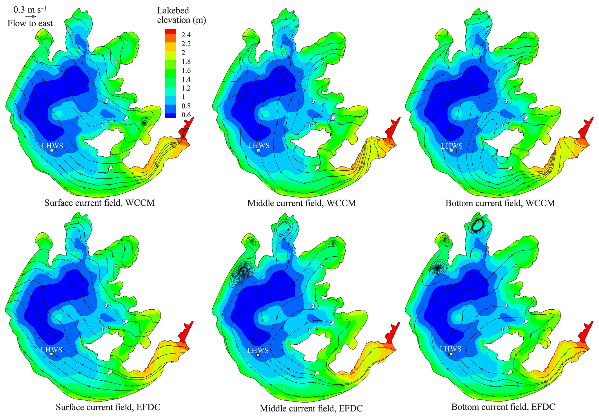
Figure B3Comparison of the flow fields and stream traces in the surface, middle, and bottom layers of Lake Taihu simulated by the WCCM and EFDC at 12:00 LT on 10 August 2015.
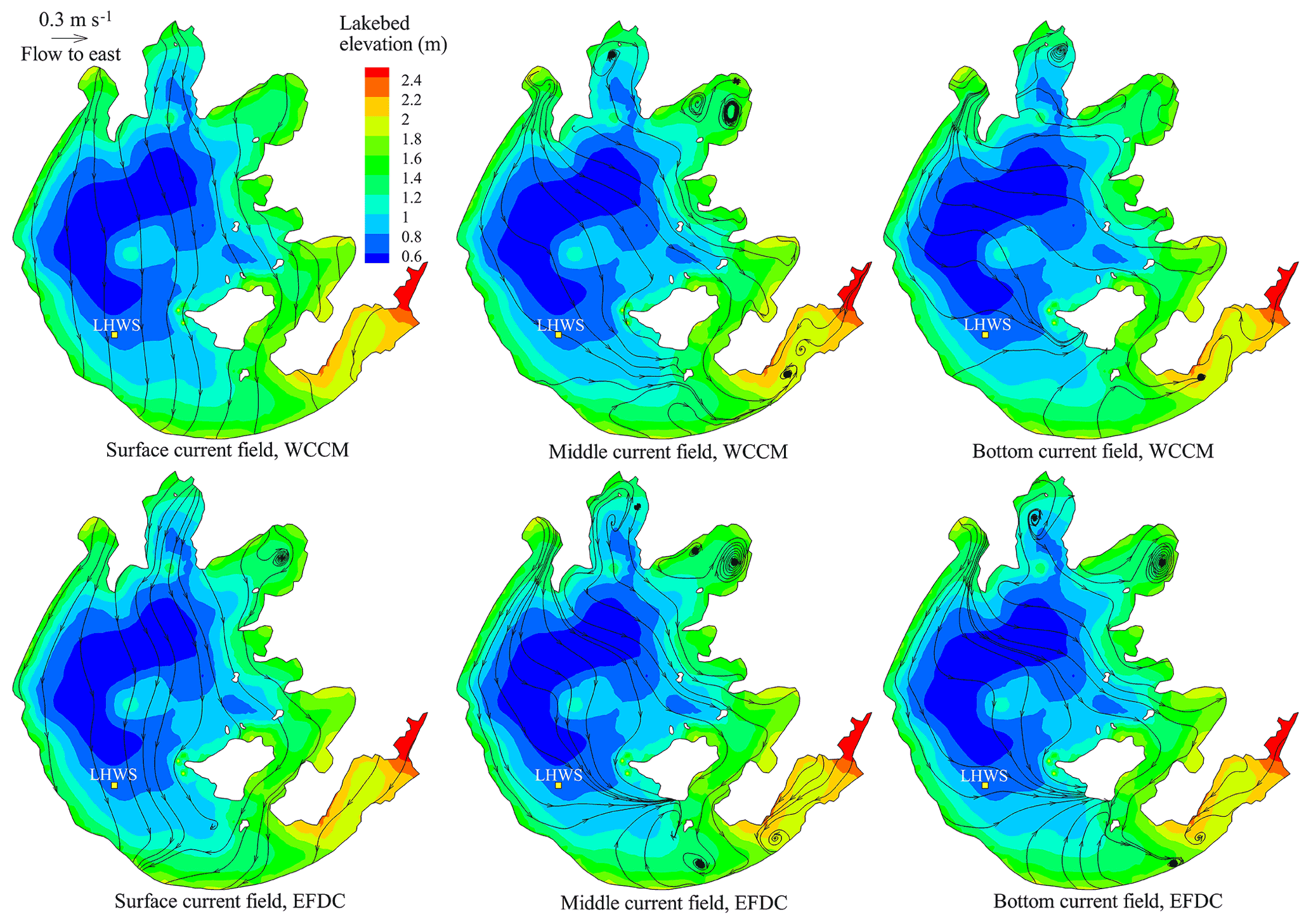
Figure B4Comparison of the flow fields and stream traces in the surface, middle, and bottom layers of Lake Taihu simulated by the WCCM and EFDC at 22:00 LT on 26 December 2018.

Figure B5Comparison of the LCM_2-simulated stream traces of the surface, middle, and bottom current fields in Lake Taihu at 12:00 LT on 10 August 2015.
The source code of the EFDC model is freely available from https://doi.org/10.5281/zenodo.5602801 (Wu, 2021a). The EFDC_Explorer 8.3 software was purchased from DSI LLC (https://www.eemodelingsystem.com/; LLC, 2021). The configurations, inputs, and outputs of the EFDC model for all simulated episodes are available from https://doi.org/10.5281/zenodo.5180640 (Wu, 2021b).
The source code of the SWAN model is freely available from http://swanmodel.sourceforge.net/ (Delft University of Technology, 2021).
The source code of the WCCM model, with the configurations, inputs, and outputs of the model as used in this paper, is freely available from https://doi.org/10.5281/zenodo.5709811 (Wu and Qin, 2021).
The dataset of measured water levels and currents is freely available from https://doi.org/10.5281/zenodo.5184459 (Hu and Wu, 2021). The other datasets used in this paper are included in the simulated episodes on Zenodo (e.g., https://doi.org/10.5281/zenodo.5180640; Wu, 2021b).
TW and BQ participated in the conceptualization, design, definition of intellectual content, literature search, model development, data acquisition and analysis, and manuscript preparation. AH, YS, and CC assisted with the model evaluation and manuscript editing. AH and SF collected significant background information and assisted with data acquisition, data analysis, and statistical analysis.
The contact author has declared that neither they nor their co-authors have any competing interests.
Publisher's note: Copernicus Publications remains neutral with regard to jurisdictional claims in published maps and institutional affiliations.
The authors thank Li Yiping from Hohai University for the determination of EFDC parameters and also James C. McWilliams from the University of California, Los Angeles, and Sun Shufen from Institute of Atmospheric Physics, Chinese Academy of Sciences for scientific suggestions.
This research has been supported by the Innovative Research Group Project of the National Natural Science Foundation of China (grant no. 41621002), the National Natural Science Foundation of China (nos. 41971047, 41790425, 41661134036), the French National Research Agency (ANR-16-CE32-0009-02), and the Water Resources Department of Jiangsu Province of China (no. 2021049).
This paper was edited by Simone Marras and reviewed by two anonymous referees.
Ardhuin, F., Jenkins, A. D., and Belibassakis, K. A.: Comments on “The three-dimensional current and surface wave equations”, J. Phys. Oceanogr., 38, 1340–1350, 2008.
Blumberg, A. F. and Mellor, G. L.: A description of a three-dimensional coastal ocean circulation model, in: Three-dimensional Coastal Ocean Models, edited by: Heaps, N., 4, 1–16, https://doi.org/10.1029/CO004, 1987.
Booij, N., Ris, R. C., and Holthuijsen, L. H.: A third-generation wave model for coastal regions, Part I, Model description and validation, J. Geophys. Res.-Oceans, 104, 7649–7666, 1999.
Butler, H. L.: Evolution of a Numerical Model for Simulating Long-Period Wave Behavior in Ocean-Estuarine Systems, in: Estuarine and Wetland Processes, edited by: Hamilton, P. and Macdonald, K. B., Marine Science, 11, Springer, Boston, MA, https://doi.org/10.1007/978-1-4757-5177-2_6, 1980.
Chen, C., Huang, H., Beardsley, R. C., Xu, Q., Limeburner, R., Cowles, G. W., Sun, Y., Qi, J., and Lin, H.: Tidal dynamics in the Gulf of Maine and New England Shelf: An application of FVCOM, J. Geophys. Res., 116, C12010, https://doi.org/10.1029/2011JC007054, 2011.
Chen, F., Zhang, C., Brett, M. T., and Nielsen, J. M.: The importance of the wind-drag coefficient parameterization for hydrodynamic modeling of a large shallow lake, Ecol. Inform., 59, 101106, https://doi.org/10.1016/j.ecoinf.2020.101106, 2020.
Chen, T., Zhang, Q., Wu, Y., Ji, C., Yang, J., and Liu, G.: Development of a wave-current model through coupling of FVCOM and SWAN, Ocean Eng., 164, 443–454, 2018.
Coastal Engineering Research Center: Shore protection manual, Dept. of the Army, Waterways Experiment Station, Corps of Engineers, Coastal Engineering Research Center, Vicksburg, Mississippi, USA, https://usace.contentdm.oclc.org/digital/collection/p16021coll11/id/1934/ (last access: 25 January 2022), 1984.
Delft University of Technology: SWAN, Delft University of Technology [code], http://swanmodel.sourceforge.net/, last access: 2 September 2021.
Edson, J. B., Jampana, V., Weller, R. A., Bigorre, S. P., Plueddemann, A. J., and Fairall, C. W., Miller, S. D., Mahrt, L., Vickers, D., and Hersbach, H.: On the exchange of momentum over the open ocean, J. Phys. Oceanogr., 43, 1589–1610, 2013.
Feng, T., Wang, C., Wang, P., Qian, J., and Wang, X.: How physiological and physical processes contribute to the phenology of cyanobacterial blooms in large shallow lakes: a new Euler-Lagrangian coupled model, Water Res., 140, 34–43, 2018.
Geernaert, G. L., Larssen, S. E., and Hansen, F.: Measurements of the wind-stress, heat flux, and turbulence intensity during storm conditions over the North Sea, J. Geophys. Res.-Oceans, 98, 16571–16582, 1987.
Hamrick, J. M.: A Three-Dimensional Environmental Fluid Dynamics Computer Code: Theoretical and Computational Aspects, Special Report No. 317 in Applied Marine Science and Ocean Engineering, College of William and Mary, Virginia Institute of Marine Science, William & Mary, https://doi.org/10.21220/V5TT6C, 1992.
Han, Y., Fang, H., Huang, L., Li, S., and He, G.: Simulating the distribution of Corbicula fluminea in Lake Taihu by benthic invertebrate biomass dynamic model (BIBDM), Ecol. Model., 409, 108730, https://doi.org/10.1016/j.ecolmodel.2019.108730, 2019.
Hipsey, M. R., Bruce, L. C., Boon, C., Busch, B., Carey, C. C., Hamilton, D. P., Hanson, P. C., Read, J. S., de Sousa, E., Weber, M., and Winslow, L. A.: A General Lake Model (GLM 3.0) for linking with high-frequency sensor data from the Global Lake Ecological Observatory Network (GLEON), Geosci. Model Dev., 12, 473–523, https://doi.org/10.5194/gmd-12-473-2019, 2019.
Hofmann, H., Lorke, A., and Peeters, F.: The relative importance of wind and ship waves in the littoral zone of a large lake, Limnol. Oceanogr., 53, 368–380, 2008.
Huang, A., Rao, Y. R., Lu, Y., and Zhao, J.: Hydrodynamic modeling of Lake Ontario: An intercomparison of three models, J. Geophys. Res.-Oceans, 115, C12076, https://doi.org/10.1029/2010JC006269, 2010.
Hu, R. and Wu, T.: Measured hydrodynamic datesets, Zenodo [data set], https://doi.org/10.5281/zenodo.5184459, 2021.
Hu, W., JØrgensen, S. E., and Zhang, F.: A vertical-compressed three-dimensional ecological model in Lake Taihu, China, Ecol. Model., 190, 367–398, 2006.
Hutter, K., Wang, Y., and Chubarenko, I. P.: Physics of lakes, Volume 1: foundation of the mathematical and physical background, edited by: Steeb, H., Advances in Geophysical and Environmental Mechanics and Mathematics book series (AGEM), Springer, ISBN 978 3 642 26597 6, 2011.
Ishikawa, M., Gonzalez, W., Golyjeswski, O., Sales, G., Rigotti, J. A., Bleninger, T., Mannich, M., and Lorke, A.: Effects of dimensionality on the performance of hydrodynamic models, Geosci. Model Dev. Discuss. [preprint], https://doi.org/10.5194/gmd-2021-250, in review, 2021.
Jeffreys, H.: On the formation of wave by wind, P. Roy. Soc. A, 107, 189–206, 1925.
Ji, C., Zhang, Q., and Wu, Y.: Derivation of three-dimensional radiation stress based on Lagrangian solutions of progressive waves, J. Phys. Oceanogr., 47, 2829–2842, https://doi.org/10.1175/JPO-D-16-0277.1, 2017.
Ji, Z. G.: Hydrodynamics and Water Quality: Modeling Rivers, Lakes, and Estuaries, 2nd Edn., John Wiley and Sons, Inc., Hoboken, New Jersey, USA, https://doi.org/10.1002/9781119371946, 2008.
Ji, Z. G., Morton, M. R., and Hamrick, J. M.: Wetting and drying simulation of estuarine processes, Estuar. Coast. Shelf S., 53, 683–700, 2001.
Jin, K. R. and Ji, Z. G.: Application and validation of three-dimensional model in a shallow lake, J. Waterway, Port, Coastal, Ocean Eng., 131, 213–225, https://doi.org/10.1061/(ASCE)0733-950X(2005)131:5(213), 2005.
Jin, K. R., Hamrick, J. H., and Tisdale, T.: Application of three-dimensional model for Lake Okeechobee, J. Hydraul. Eng., 126, 758–771, 2000.
Koue, J., Shimadera, H., Matsuo, T., and Kondo, A.: Evaluation of thermal stratification and flow field reproduced by a three-dimensional hydrodynamic model in Lake Biwa, Japan, Water, 10, 47, https://doi.org/10.3390/w10010047, 2018.
Kumar, N., Voulgaris, G., and Warner, J. C.: Implementation and modification of a three-dimensional radiation stress formulation for surf zone and rip-current applications, Coast. Eng., 58, 1097–1117, 2011.
Large, W. G. and Pond, S.: Open ocean momentum flux measurements in moderate to strong winds, J. Phys. Oceanogr., 11, 324–336, 1981.
LLC: Dynamic Solutions – International, LLC [code], https://www.eemodelingsystem.com/, last access: 7 August 2021.
Longuet-Higgins, M. S. and Stewart, R. W.: Radiation stresses in water waves: a physical discussion, with application, Deep-Sea Res., 11, 529–562, 1964.
Li, Y., Acharya, K., and Yu, Z.: Modeling impacts of Yangtze River water transfer on water ages in Lake Taihu, China, Ecol. Eng., 37, 325–334, 2011.
Li, Y., Tang, C., Zhu, J., Pan, B., Anim, D. O., Ji, Y., Yu, Z., and Acharya, K.: Parametric uncertainty and sensitivity analysis of hydrodynamic processes for a large shallow freshwater lake, Hydrolog. Sci. J., 60, 1078–1095, 2015.
Liu, B., Liu, H., Xie, L., Guan, C., and Zhao, D.: A coupled atmosphere-wave-ocean modeling system: simulation of the intensity of an idealized tropical cyclone, Mon. Weather Rev., 139, 132–152, 2011.
Liu, S., Ye, Q., Wu, S., and Stive, M. J. F.: Horizontal Circulation Patterns in a Large Shallow Lake: Taihu Lake, China, Water, 10, 792, https://doi.org/10.3390/w10060792, 2018.
Lükő, G., Torma, P., Krámer, T., Weidinger, T., Vecenaj, Z., and Grisogono, B.: Observation of wave-driven air–water turbulent momentum exchange in a large but fetch-limited shallow lake, Adv. Sci. Res., 17, 175–182, https://doi.org/10.5194/asr-17-175-2020, 2020.
MacIntyre, S., Bastviken, D., Arneborg, L., Crowe, A. T., Karlsson, J., Andersson A., Gålfalk, M., Rutgersson, A., Podgrajsek, E., and Melack, J. M.: Turbulence in a small boreal lake: Consequences for air-water gas exchange, Limnol. Oceanogr., 9999, 1–28, https://doi.org/10.1002/lno.11645, 2020.
Mao, J., Chen, Q., and Chen, Y.: Three-dimensional eutrophication model and application to Lake Taihu, China, J. Environ. Sci., 20, 278–284, 2008.
Mellor, G. L.: The depth-dependent current and wave interaction equations: a revision, J. Phys. Oceanogr., 38, 2587–2596, 2008.
Mellor, G. L. and Yamada, T.: Development of a turbulence closure model for geophysical fluid problems, Rev. Geophys. Space Phys., 20, 851–875, 1982.
Morey, S. L., Gopalakrishnan, G., Sanz, E. P., De Souza, J. M. A. C., Donohue, K., Pérez-Brunius, P., Dukhovskoy, D., Chassignet, E., Cornuelle, B., Bower, A., Furey, H., Hamilton, P., and Candela, J.: Assessment of numerical simulations of deep circulation and variability in the Gulf of Mexico using recent observations, J. Phys. Oceanogr., 50, 1045–1064, 2020.
Munk, W. H.: Wind stress on water: an hypothesis, Q. Roy. Meteor. Soc., 81, 320–332, https://doi.org/10.1002/qj.49708134903, 1955.
Qin, B., Xu, P., Wu, Q., Luo, L., and Zhang, Y.: Environmental issues of Lake Taihu, China, Hydrobiologia, 581, 3–14, 2007.
Rey, A., Mulligan, R., Filion, Y., da Silva, A. M., Champagne, P. and Boegman, L.: Three-dimensional hydrodynamic behaviour of an operational wastewater stabilization pond, J. Environ. Eng. ASCE, 147, 05020009, https://doi.org/10.1061/(ASCE)EE.1943-7870.0001834, 2021.
Schoen, J. H., Stretch, D. D., and Tirok, K.: Wind-driven circulation patterns in a shallow estuarine lake: St Lucia, South Africa, Estuar. Coast. Shelf S., 146, 49–59, 2014.
Shchepetkin, A. F. and McWilliams, J. C.: The regional oceanic modeling system (ROMS): a split-explicit, free-surface, topography-following-coordinate oceanic model, Ocean Model., 9, 347–404, 2005.
Soulignac, F., Vinçon-Leite, B., Lemaire, B. J., Martins, J. R., Scarati, Bonhomme, C., Dubois, P., Mezemate, Y., Tchiguirinskaia, I., Schertzer, D., and Tassin, B.: Performance assessment of a 3D hydrodynamic model using high temporal resolution measurements in a shallow urban lake, Environ. Model. Assess., 22, 309–322, 2017.
Sun, F., Wei, Y., and Wu, K.: Wave-induced radiation stress under geostrophic condition, Acta Oceanol. Sin., 28, 1–4, 2006 (in Chinese with English abstract).
SWAN team: SWAN Cycle III version 41.31AB, Use Manual, Delft University of Technology, 2600 GA DELFT, Netherlands, https://swanmodel.sourceforge.io/download/download.htm (last access: 2 September 2021), 2021.
Vinçon-Leite, B. and Casenave, C.: Modelling eutrophication in lake ecosystems: A review, Sci. Total Environ., 651, 2985–3001, 2019.
Wang, C., Shen, C., Wang, P. F., Qian, J., Hou, J., and Liu, J. J.: Modeling of sediment and heavy metal transport in Taihu Lake, China, J. Hydrodyn. Ser. B, 25, 379–387, 2013.
Wang, Z., Wu, T., Zou, H., Jia, X., Huang, L., Liang, C., and Zhang, Z.: Changes in seasonal characteristics of wind and wave in different regions of Lake Taihu, J. Lake Sci., 28, 217–224, 2016 (in Chinese with English abstract).
Warner, J. C., Sherwood, C. R., Signell, R. P., Harris, C. K., and Arango, H. G.: Development of a three-dimensional, regional, coupled wave, current, and sediment-transport model, Comput. Geosci., 34, 1284–1306, 2008.
Wei, Z., Miyano, A., and Sugita, M.: Drag and bulk transfer coefficients over water surfaces in light winds, Bound.-Lay. Meteorol., 160, 319–346, 2016.
Wu, J.: Wind-stress coefficients over sea surface near neutral conditions – A revisit, J. Phys. Oceanogr., 10, 727–740, 1980.
Wu, L., Chen, C., Guo, P., Shi, M., Qi, J., and Ge, J.: A FVCOM-based unstructured grid wave, current, sediment transport model, I. model description and validation, J. Ocean U. China, 10, 1–8, 2011.
Wu, T.: The source code of the EFDC model, Zenodo [code], https://doi.org/10.5281/zenodo.5602801, 2021a.
Wu, T.: The configurations, inputs and outputs of the EFDC model for all simulated episodes, Zenodo [data set], https://doi.org/10.5281/zenodo.5180640, 2021b.
Wu, T. and Qin, B.: The configurations, inputs and outputs of the WCCM model for all simulated episodes, Zenodo [code], https://doi.org/10.5281/zenodo.5709811, 2021.
Wu, T., Qin, B., Ding, W., Zhu, G., Zhang, Y., Gao, G., Xu, H., Li, W., Dong, B., and Luo, L.: Field observation of different wind-induced basin-scale current field dynamics in a large, polymictic, eutrophic lake, J. Geophys. Res.-Oceans, 123, 6945–6961, 2018.
Wu, T., Qin, B., Brookes, J. D., Yan, W., Ji, X., Feng, J., Ding, W., and Wang, H.: Spatial distribution of sediment nitrogen and phosphorus in Lake Taihu from a hydrodynamics-induced transport perspective, Sci. Total Environ., 650, 1554–1565, 2019.
Wüest, A. and Lorke, A.: Small-scale hydrodynamics in lakes, Annu. Rev. Fluid Mech., 35, 373–412, 2003.
Xiao, W., Liu, S., Wang, W., Yang, D., Xu, J., Cao, C., Li, H., and Lee, X.: Transfer coefficients of momentum, heat and water vapour in the atmospheric surface layer of a large freshwater lake, Bound.-Lay. Meteorol., 148, 479–494, https://doi.org/10.1007/s10546-013-9827-9, 2013.
Xu, X., Tao, R., Zhao, Q., and Wu, T.: Wave characteristics and sensitivity analysis of wind field in a large shallow lake-Lake Taihu, J. Lake Sci., 25, 55–64, 2013 (in Chinese with English abstract).
Xu, Z. G. and Bowen, A. J.: Wave- and wind-driven flow in water of finite depth, J. Phys. Oceanogr., 24, 1850–1866, 1994.
Zhao, Q., Sun, J., and Zhu, G.: Simulation and exploration of the mechanisms underlying the spatiotemporal distribution of surface mixed layer depth in a large shallow lake, Adv. Atmos. Sci., 29, 1360–1373, https://doi.org/10.1007/s00376-012-1262-1, 2012.
Zheng, S., Wang, P., Wang, C., and Hou, J.: Sediment resuspension under action of wind in Taihu Lake, China, Int. J. Sediment Res., 30, 48–62, 2015.
Zhou, J., Zeng, C., and Wang, L.: Influence of wind drag coefficient on wind-drived flow simulation, Chinese J. Hydrodyn., 24, 440–447, 2009 (in Chinese with English abstract).
Zhou, L., Chen, D., Karnauskas, K. B., Wang, C., Lei, X., Wang, W., Wang, G., and Han, G.: Introduction to special section on oceanic responses and feedbacks to tropical cyclones, J. Geophys. Res.-Oceans, 123, 742–745, https://doi.org/10.1002/2018JC013809, 2018.