The Moist Quasi-Geostrophic Coupled Model: MQ-GCM 2.0

This paper contains a description of recent changes to the formulation and numerical implementation of the Quasi-Geostrophic Coupled Model (Q-GCM), which constitute a major update of the previous version of the model (Hogg et al., 2014). The Q-GCM model has been designed to provide an efficient numerical tool to study the dynamics of multi-scale midlatitude air–sea interactions and their climatic impacts. The present additions/alterations were motivated by an inquiry into the dynamics of mesoscale ocean–atmosphere coupling and, in particular, by an apparent lack of the Q-GCM atmosphere's sensitivity to mesoscale sea-surface temperature (SST) anomalies, even at high (mesoscale) atmospheric resolutions, contrary to ample theoretical and observational evidence otherwise. Major modifications aimed at alleviating this problem include an improved radiative-convective scheme resulting in a more realistic model mean state and associated model parameters; a new formulation of entrainment in the atmosphere, which prompts more efficient communication between the atmospheric mixed layer and free troposphere; and an addition of a temperature-dependent wind component in the atmospheric mixed layer and the resulting mesoscale feedbacks. The most drastic change is, however, the inclusion of moist dynamics in the model, which may be key to midlatitude ocean–atmosphere coupling. Accordingly, this version of the model is to be referred to as the MQ-GCM model. Overall, the MQ-GCM model is shown to exhibit a rich spectrum of behaviors reminiscent of many of the observed properties of the Earth's climate system. It remains to be seen whether the added processes are able to affect in fundamental ways the simulated dynamics of the midlatitude ocean–atmosphere system's coupled decadal variability.

1 Introduction

The Quasi-Geostrophic Coupled Model (Q-GCM) was initially developed by Hogg et al. (2003) and has been substantially modified since its latest distribution and source code are publicly available at http://www.q-gcm.org (last access: 10 May 2022; publicly available indefinitely) and are fully documented in the Q-GCM users' guide, v1.5.0 (Hogg et al., 2014). The model couples the multi-layer quasi-geostrophic (QG) ocean and atmosphere components via ageostrophic mixed layers that regulate the exchange of heat and momentum between the two fluids. Q-GCM model can be configured as either a box (double gyre) or a channel ocean (Southern Ocean) underneath a channel atmosphere; it conceptualizes the midlatitude climate system driven by the latitudinal variation of the incoming solar radiation. In addition to the oceanic mixed layer, the model physics incorporates a dynamically active atmospheric mixed layer (effectively, the atmospheric planetary boundary layer: APBL), the dependence of the wind stress on the ocean–atmosphere surface velocity difference, and a dynamically consistent parameterization of the entrainment heat fluxes between the model layers. It can also be easily modified to include a parameterization of a sea-surface temperature (SST) feedback on the wind stress (e.g., Hogg et al., 2009), which will be a part of the new version of the model developed here. Q-GCM thus encompasses a richer, more comprehensive set of processes, enabling one to achieve a more accurate simulation of the ocean–atmosphere coupling, especially at mesoscales, relative to some other analogous conceptual models, which either assume the atmospheric near-surface temperature to be in equilibrium with SST (e.g., Feliks et al., 2004, 2007, 2011; cf. Schneider and Qiu, 2015) or relate this temperature in an ad hoc way to the instantaneous in situ distribution of the model's tropospheric temperature (Kravtsov et al., 2005, 2006, 2007; Deremble et al., 2012). The Q-GCM model was previously used for ocean-only and coupled experiments around the double-gyre problem (Hogg et al., 2005, 2006, 2007; Martin et al., 2020), as well as in the ocean-only studies of the Southern Ocean's climate system (Hogg and Blundell, 2006; Meredith and Hogg, 2006; Hogg et al., 2008; Hutchinson et al., 2010; Kravtsov et al., 2011).

The long oceanic thermal and dynamical inertia makes the ocean a primary agent for generating potentially predictable climate signals on timescales from years to decades, whereas atmospheric intrinsic timescales are significantly shorter. The null hypothesis for climate variability views the ocean as a passive integrator of high-frequency noise associated with atmospheric geostrophic turbulence (Hasselmann, 1976; Frankignoul and Hasselmann, 1977; Frankignoul, 1985; Barsugli and Battisti, 1998; Xie, 2004). However, both observations (e.g., Chelton, 2013; Frenger et al., 2013) and decades of experimentation with wind-driven eddy-resolving ocean models (e.g., Berloff and McWilliams, 1999; Primeau, 2002; Berloff et al., 2007; Hogg et al., 2009; Shevchenko et al., 2016, among many others) documented vigorous internal variability and the associated mesoscale features (fronts and eddies with spatial scales of 10–100 km) throughout the world ocean. Two key regions in which these eddies are most important are near the western boundary currents and their extensions and in the Southern Ocean. Mesoscale variability in these regions modulates atmospheric fronts and storms' intensity and distribution, thus affecting atmospheric variability on short timescales (e.g., Maloney and Chelton, 2006; Minobe et al., 2008; Nakamura and Yamane, 2009; Bryan et al., 2010; Chelton and Xie, 2010; Kuwano-Yoshida et al., 2010; O'Neill et al., 2010, 2012; Frenger et al., 2013; O'Reilly and Czaja, 2015; Seo et al., 2016; Parfitt et al., 2017). Recent observational and modeling evidence strongly suggested that this mesoscale oceanic turbulence may also imprint itself onto large-scale low-frequency climate modes (with timescales from intra-seasonal to decadal), which would have profound consequences for near-term climate predictability (e.g., Hogg et al., 2006; Siqueira and Kirtman, 2016). To study this phenomenon may, therefore, require coupled climate models with high horizontal resolution in both their oceanic and atmospheric components (see below); this would make the requisite long climate simulations using highly resolved state-of-the-art climate models computationally infeasible.

Feliks et al. (2004, 2007, 2011) and Brachet et al. (2012) examined the response of the atmosphere-to-mesoscale sea-surface temperature (SST) anomalies through hydrostatic pressure adjustment in an idealized atmospheric model. They showed that resolving an ocean front and mesoscale eddies affects atmospheric climatology, intraseasonal modes, and decadal variability (when forced with the observed SST history) in their model (see also Nakamura et al., 2008). These authors argued that atmospheric components of global climate models must resolve oceanic fronts to faithfully simulate the observed climate variability (see also Minobe et al., 2008). Ma et al. (2017) also concluded that “It is only when the (atmospheric) model has sufficient resolution to resolve small-scale diabatic heating that the full effect of mesoscale SST forcing on the storm track can be correctly simulated,” with the ensuing consequences for atmospheric low-frequency variability associated with the downstream Rossby wave breaking (Piazza et al., 2016) and blocking (O'Reilly et al., 2015). By contrast, Bryan et al. (2010) proposed that accurate representation of mesoscale ocean–atmosphere coupling in a model depends more on the marine atmospheric boundary layer (MABL) mixing scheme than on the ability of an atmospheric model to resolve a thermal front per se; this would justify the use of atmospheric resolutions on the order of 50 km in many general circulation model studies that documented a pronounced influence of the mesoscale air–sea interactions on the atmospheric storm tracks (Miller and Schneider, 2000; Nakamura et al., 2008; Taguchi et al., 2009; Kelly et al., 2010; Perlin et al., 2014; Small et al., 2014; Ma et al., 2015, 2017; Piazza et al., 2016).

A numerically efficient intermediate-complexity Q-GCM model thus provides an alternative (to highly resolved general circulation models) and unique tool ideally suited to help advance our understanding of multi-scale ocean–atmosphere interactions and their climatic impacts. Its QG dynamical core resolves well the geostrophic turbulence on either side of the ocean–atmosphere interface, including oceanic mesoscale eddies/fronts and atmospheric storm tracks. The existing version of the coupled model, however, lacks the parameterization of SST effects on the model's MABL winds. One such parameterization was tested in the Q-GCM's ocean-only configuration by Hogg et al. (2009). Mastilovic and Kravtsov (2019) examined the effects of both Hogg et al. (2009) and Feliks et al.'s (2004, 2007) SST-dependent MABL wind formulations in the context of coupled Q-GCM simulations with the standard (coarse) and fine (mesoscale resolving) atmospheric grid spacing. They found that – consistent with previous studies (Dewar and Flierl, 1987; Maloney and Chelton, 2006; Hogg et al., 2009; Gaube et al., 2013, 2015; Chelton, 2013; Small et al., 2014) – these effects constitute a negative feedback on the ocean and tend to reduce the intensity of the oceanic mesoscale perturbations that generated the mesoscale wind anomalies in the first place. In a coupled setting, this leads to a dilution of oceanic mesoscale features and the resulting lack of the model's sensitivity to atmospheric resolution. Surprisingly, the atmosphere-only Q-GCM simulations with and without an SST front, or with and without SST-dependent MABL winds, apparently also produce statistically identical atmospheric variability irrespective of the atmospheric resolution (Ilijana Mastilovic and Sergey Kravtsov, personal communication, 2020), in sharp contrast to the resolution-dependent dynamics documented in Feliks et al. (2004, 2007). Furthermore, the entire previous experience with Q-GCM indicates the absence, in the existing version of the model, of a nonlinear, weather-regime-type atmospheric behavior documented in analogous atmospheric (Marshall and Molteni, 1993; Kravtsov et al., 2005) and coupled models (Kravtsov et al., 2006, 2007); such behavior may lead to a nonlinear atmospheric sensitivity to ocean-induced SST anomalies and generate fundamentally coupled decadal climate modes (e.g., Kravtsov et al., 2008).

The purpose of this paper is to document a new, revamped version of the Q-GCM model, which addresses an apparent lack of the Q-GCM atmosphere's sensitivity to SST anomalies, contrary to ample theoretical and observational evidence otherwise. In Sect. 2, we briefly summarize the dynamical (QG) core of the model, placing some of the supporting information in the Appendix. Major modifications to the original, dry-model physics (Sect. 3) include an improved radiative-convective scheme resulting in a more realistic model mean state and the associated model parameters; a new formulation of entrainment in the atmosphere, which prompts a more efficient communication between the atmospheric mixed layer and free troposphere; and an addition of a temperature-dependent wind component in the atmospheric mixed layer and the resulting mesoscale feedbacks. The most drastic change is, however, the inclusion, in the model, of moist dynamics (Sect. 4), which may be key to midlatitude ocean–atmosphere coupling (Czaja and Blunt, 2011; Laîné et al., 2011; Deremble et al., 2012; Willison et al., 2013; Foussard et al., 2019). Accordingly, this version of the model is to be referred to as the MQ-GCM model. Overall, the MQ-GCM model is shown to exhibit a rich spectrum of behaviors reminiscent of many of the observed properties of the Earth's climate system (Sect. 5). The paper concludes with some discussion in Sects. 6 and 7, which summarizes the MQ-GCM changes and code modifications with respect to the original Q-GCM version. This presentation is also supplemented with the collection of Fortran 90 routines containing all the new MQ-GCM source code that complement the original Q-GCM distribution (http://www.q-gcm.org, last access: 10 May 2022).

2 Q-GCM dynamical core

Q-GCM model incorporates quasi-geostrophic dynamics on a β-plane in its n-layer oceanic and atmospheric modules (below, we will use n=3); these dynamics are governed by the equations describing the evolution of quasi-geostrophic potential vorticity q. For a flat-bottom ocean (used here for simplicity, although the topography is included in Q-GCM),

$$\begin{array}{}\text{(1)}& \begin{array}{rl}{}^{\mathrm{o}}{q}_{k_t}& +J\left({}^{\mathrm{o}}{\mathit{\psi }}_k,{}^{\mathrm{o}}{q}_k\right)={\displaystyle \frac{f_{\mathrm{0}}}{{}^{\mathrm{o}}{H}_k}}\left({}^{\mathrm{o}}{e}_{k-\mathrm{1}}-{}^{\mathrm{o}}{e}_k\right)+{}^{\mathrm{o}}{A}_{\mathrm{2}}\mathrm{\nabla }{}_H^{\mathrm{4}}{}^{\mathrm{o}}{\mathit{\psi }}_k\\ & -{}^{\mathrm{o}}{A}_{\mathrm{4}}\mathrm{\nabla }{}_H^{\mathrm{6}}{}^{\mathrm{o}}{\mathit{\psi }}_k;k=\mathrm{1},\mathrm{2},\mathrm{3},\end{array}\end{array}$$

where

$$\begin{array}{}\text{(2)}& \begin{array}{rl}{}^{\mathrm{o}}{q}_k& ={\mathrm{\nabla }}_H^{\mathrm{2}}{}^{\mathrm{o}}{\mathit{\psi }}_k+{\displaystyle \frac{f_{\mathrm{0}}}{{}^{\mathrm{o}}{H}_k}}\left({}^{\mathrm{o}}{\mathit{\eta }}_k-{}^{\mathrm{o}}{\mathit{\eta }}_{k-\mathrm{1}}\right)\\ & +\mathit{\beta }\left(y-y_o\right);k=\mathrm{1},\mathrm{2},\mathrm{3}\end{array}\end{array}$$

and

$$\begin{array}{}\text{(3)}& \begin{array}{rl}{}^{\mathrm{o}}{\mathit{\eta }}_k& ={\displaystyle \frac{f_{\mathrm{0}}}{{}^{\mathrm{o}}{g}_k^{\prime }}}\left({}^{\mathrm{o}}{\mathit{\psi }}_{k+\mathrm{1}}-{}^{\mathrm{o}}{\mathit{\psi }}_k\right),{}^{\mathrm{o}}{g}_k^{\prime }=g{\displaystyle \frac{({}^{\mathrm{o}}{\mathit{\rho }}_{k+\mathrm{1}}-{}^{\mathrm{o}}{\mathit{\rho }}_k)}{{}^{\mathrm{o}}{\mathit{\rho }}_{\mathrm{0}}}};\\ k& =\mathrm{1},\mathrm{2};{}^{\mathrm{o}}{\mathit{\eta }}_{\mathrm{0}}={}^{\mathrm{o}}{\mathit{\eta }}_{\mathrm{3}}=\mathrm{0}.\end{array}\end{array}$$

In the equations above, the left superscript “o” refers to the oceanic quantities, ^oq_k is the potential vorticity for ocean layer k, counted from the surface down, ^oψ_k is the layer-k geostrophic streamfunction, ^oH_k represents the layer thicknesses, and ^oq_k represents the layer densities (all close to the representative water density ^oρ₀), with $k=\mathrm{1},\mathrm{2},\mathrm{3}$. Furthermore, ^oη_k represents the perturbation displacements of the interface between the top/middle and middle/bottom layers; ${}^{\mathrm{o}}{g}_k^{\prime }$ represents the reduced gravity coefficients (for both of these $k=\mathrm{1},\mathrm{2}$); f₀ and β are the Coriolis parameter and its y derivative at the central latitude y₀, respectively; ^oA₂ and ^oA₄ are viscosity coefficients for the Laplacian and biharmonic friction parameterizations; the subscript t denotes the time derivative; ${\mathrm{\nabla }}_H^{\mathrm{2}}$ is the horizontal Laplacian operator; and J is the Jacobian operator. The ocean model is driven by the entrainment ^oe₀=^ow_ek associated with the surface Ekman pumping ^ow_ek computed as the curl of the wind stress; the model also includes Ekman dissipation at the bottom, with ${}^{\mathrm{o}}{e}_{\mathrm{3}}\sim {\mathrm{\nabla }}_H^{\mathrm{2}}{}^{\mathrm{o}}{\mathit{\psi }}_{\mathrm{3}}$, as well as a thermally driven entrainment ^oe₁ (between ocean layers 1 and 2) due to heat exchange between the ocean's layer 1 and the mixed layer (see Sect. 3.2 below, as well as Hogg et al., 2014, for further details).

The atmospheric module mirrors the ocean module: it is set up in a fluid comprised of layers with constant potential temperatures θ_k and variable depths (see the Appendix). In particular,

$$\begin{array}{}\text{(4)}& {\displaystyle }\begin{array}{rl}{}^{\mathrm{a}}{q}_{k_t}& +J\left({}^{\mathrm{a}}{\mathit{\psi }}_k,{}^{\mathrm{a}}{q}_k\right)={\displaystyle \frac{f_{\mathrm{0}}}{{}^{\mathrm{a}}{H}_k}}\left({}^{\mathrm{a}}{e}_k\right.\\ & \left.-{}^{\mathrm{a}}{e}_{k-\mathrm{1}}\right)-{}^{\mathrm{a}}{A}_{\mathrm{4}}{\mathrm{\nabla }}_H^{\mathrm{6}}{}^{\mathrm{a}}{\mathit{\psi }}_k;k=\mathrm{1},\mathrm{2},\mathrm{3};\end{array}\text{(5)}& {\displaystyle }\begin{array}{rl}{}^{\mathrm{a}}{q}_k& ={\mathrm{\nabla }}_H^{\mathrm{2}}{}^{\mathrm{a}}{\mathit{\psi }}_k+{\displaystyle \frac{f_{\mathrm{0}}}{{}^{\mathrm{a}}{H}_k}}\left({}^{\mathrm{a}}{\mathit{\eta }}_k-{}^{\mathrm{a}}{\mathit{\eta }}_{k-\mathrm{1}}\right)+\mathit{\beta }\left(y-y_{\mathrm{0}}\right);\\ k& =\mathrm{1},\mathrm{2},\mathrm{3};\end{array}\text{(6)}& {\displaystyle }\begin{array}{rl}{}^{\mathrm{a}}{\mathit{\eta }}_k& ={\displaystyle \frac{f_{\mathrm{0}}}{{}^{\mathrm{a}}{g}_k^{\prime }}}\left({}^{\mathrm{a}}{\mathit{\psi }}_k-{}^{\mathrm{a}}{\mathit{\psi }}_{k+\mathrm{1}}\right),{}^{\mathrm{a}}{g}_k^{\prime }=g{\displaystyle \frac{({\mathit{\theta }}_{k+\mathrm{1}}-{\mathit{\theta }}_k)}{\stackrel{\mathrm{‾}}{\mathit{\theta }}}};\\ k& =\mathrm{1},\mathrm{2};{}^{\mathrm{a}}{\mathit{\eta }}_{\mathrm{0}}={}^{\mathrm{a}}{\mathit{\eta }}_{\mathrm{3}}=\mathrm{0}.\end{array}\end{array}$$

Note that the layer indexing in the equations above goes from the surface upward and the Laplacian friction term is omitted; otherwise, these equations are completely analogous to the oceanic equations (the atmospheric variables are denoted above by the left superscript “a”). At the lower atmospheric boundary, the entrainment flux ^ae₀=^aw_ek solely represents, in the original Q-GCM formulation, Ekman dissipation (thus signifying the momentum transfer from the atmosphere to the ocean); in the modified version of the model to be developed here it will also include a temperature-dependent component capable of driving mesoscale air–sea interaction (Sect. 3.3). The atmospheric model (and thus the entire coupled model) is driven through interior entrainment fluxes ^ae₁, ^ae₂ in Eq. (4) (^ae₃ is set to zero), which are a by-product of perturbing the mean-state radiative-convective equilibrium (Sect. 3.1) by a latitudinally non-uniform insolation. The new radiation/heat exchange formulation and mixed-layer/entrainment formulation developed here (Sect. 3) are aimed to help achieve a parameter regime with enhanced (and, arguably, more realistic) coupling between oceanic and atmospheric dynamics in the model. They are further modified in formulating the new version of the model with an active hydrological cycle and the associated latent-heat feedbacks (Sect. 4).

3 Updates to the original “dry” version of Q-GCM

In describing the updates below, we will generally focus on the elements of Q-GCM model that have been revised here and quote the values of new parameters, or the updated values of the previously used parameters along the way, while referring the reader/user to the existing Q-GCM guide (Hogg et al., 2014) for a more thorough description of the default model configuration.

3.1 Radiative-convective equilibrium, atmospheric mean state, and convective fluxes

The previous version of Q-GCM assumes purely radiative equilibrium to compute the atmospheric mean state. In the revised version, this assumption is replaced by that of the radiative-convective mean-state balance. We denote the actual (not potential) vertically averaged temperatures within each of the interior atmospheric layers as ^aT_k, $k=\mathrm{1},\mathrm{2},\mathrm{3}$ to write, over ocean,

$$\begin{array}{}\text{(7)}& \begin{array}{rl}{}^{\mathrm{o}}\mathit{\rho }{}^{\mathrm{o}}{C}_p{}^{\mathrm{o}}{H}_{\mathrm{m}}{}^{\mathrm{o}}{\dot{T}}_{\mathrm{m}}& =-F_{\mathit{\lambda }}-F_{\mathrm{0}}^{\uparrow }-F_{\mathrm{m}}^{\downarrow }-F_{\mathrm{s}}+{}^{\mathrm{o}}{F}_{\mathrm{m}}^{e+},\\ {}^{\mathrm{a}}\mathit{\rho }{}^{\mathrm{a}}{C}_p{}^{\mathrm{a}}{H}_{\mathrm{m}}{}^{\mathrm{a}}{\dot{T}}_{\mathrm{m}}& =F_{\mathit{\lambda }}+F_{\mathrm{0}}^{\uparrow }+F_{\mathrm{m}}^{\downarrow }-\left(F_{\mathrm{m}}^{\uparrow }+{}^{\mathrm{a}}{F}_{\mathrm{m}}^{e-}+F_{\mathrm{1}}^{\downarrow }\right),\\ {}^{\mathrm{a}}\mathit{\rho }{}^{\mathrm{a}}{C}_p{}^{\mathrm{a}}{H}_{\mathrm{1}}{}^{\mathrm{a}}{\dot{T}}_{\mathrm{1}}& =F_{\mathrm{m}}^{\uparrow }+F_{\mathrm{1}}^{\downarrow }+{}^{\mathrm{a}}{F}_{\mathrm{m}}^{e+}-\left(F_{\mathrm{1}}^{\uparrow }+F_{\mathrm{2}}^{\downarrow }+{}^{\mathrm{a}}{F}_{\mathrm{1}}^{e-}\right),\\ {}^{\mathrm{a}}\mathit{\rho }{}^{\mathrm{a}}{C}_p{}^{\mathrm{a}}{H}_{\mathrm{2}}{}^{\mathrm{a}}{\dot{T}}_{\mathrm{2}}& =F_{\mathrm{1}}^{\uparrow }+F_{\mathrm{2}}^{\downarrow }+{}^{\mathrm{a}}{F}_{\mathrm{1}}^{e+}-\left(F_{\mathrm{2}}^{\uparrow }+F_{\mathrm{3}}^{\downarrow }+{}^{\mathrm{a}}{F}_{\mathrm{2}}^{e-}\right),\\ {}^{\mathrm{a}}\mathit{\rho }{}^{\mathrm{a}}{C}_p{}^{\mathrm{a}}{H}_{\mathrm{3}}{}^{\mathrm{a}}{\dot{T}}_{\mathrm{3}}& =F_{\mathrm{2}}^{\uparrow }+F_{\mathrm{3}}^{\downarrow }+{}^{\mathrm{a}}{F}_{\mathrm{2}}^{e+}-F_{\mathrm{3}}^{\uparrow }.\end{array}\end{array}$$

Here the dot denotes the time derivative and other notations follow the Q-GCM users' guide, v1.5.0 (Hogg et al., 2014). In particular, the upward/downward arrow subscripts denote upwelling/downwelling longwave radiative fluxes within each of the layers k=m (mixed layer), 1, 2, 3 or the surface (0); the subscripts e− and e+ denote entrainment fluxes below and above interface k; the subscript s refers to the solar radiation; and λ refers to the ocean–atmosphere sensible/latent-heat exchange. The fluxes describing non-radiative heat exchange between the layers are interpreted, in the mean state, as convective fluxes parameterized in the following way (cf. Manabe and Strickler, 1964; Manabe and Wetherald, 1967; Ramanathan and Coakley, 1978):

$$\begin{array}{}\text{(8)}& \begin{array}{rl}\stackrel{\mathrm{‾}}{F_{\mathit{\lambda }}}& =K\left({}^{\mathrm{o}}\stackrel{\mathrm{‾}}{T_{\mathrm{m}}}-{}^{\mathrm{a}}\stackrel{\mathrm{‾}}{T_{\mathrm{m}}}-{\mathit{\gamma }}_{\mathrm{c}}\mathrm{\Delta }{H}_{\mathrm{m}}\right);\\ \mathrm{\Delta }{H}_{\mathrm{m}}& ={}^{\mathrm{a}}{H}_{\mathrm{m}}/\mathrm{2},\\ {}^{\mathrm{a}}\stackrel{\mathrm{‾}}{F_{\mathrm{m}}^e}& ={}^{\mathrm{a}}\stackrel{\mathrm{‾}}{F_{\mathrm{m}}^{e-}}={}^{\mathrm{a}}\stackrel{\mathrm{‾}}{F_{\mathrm{m}}^{e+}}=K\left({}^{\mathrm{a}}\stackrel{\mathrm{‾}}{T_{\mathrm{m}}}-{}^{\mathrm{a}}\stackrel{\mathrm{‾}}{T_{\mathrm{1}}}-{\mathit{\gamma }}_{\mathrm{c}}\mathrm{\Delta }{H}_{\mathrm{1}}\right);\\ \mathrm{\Delta }{H}_{\mathrm{1}}& =\left({}^{\mathrm{a}}{H}_{\mathrm{m}}+{}^{\mathrm{a}}{H}_{\mathrm{1}}\right)/\mathrm{2},\\ {}^{\mathrm{a}}\stackrel{\mathrm{‾}}{F_{\mathrm{1}}^e}& ={}^{\mathrm{a}}\stackrel{\mathrm{‾}}{F_{\mathrm{1}}^{e-}}={}^{\mathrm{a}}\stackrel{\mathrm{‾}}{F_{\mathrm{1}}^{e+}}=K\left({}^{\mathrm{a}}\stackrel{\mathrm{‾}}{T_{\mathrm{1}}}-{}^{\mathrm{a}}\stackrel{\mathrm{‾}}{T_{\mathrm{2}}}-{\mathit{\gamma }}_{\mathrm{c}}\mathrm{\Delta }{H}_{\mathrm{2}}\right);\\ \mathrm{\Delta }{H}_{\mathrm{2}}& =\left({}^{\mathrm{a}}{H}_{\mathrm{1}}+{}^{\mathrm{a}}{H}_{\mathrm{2}}\right)/\mathrm{2},\\ {}^{\mathrm{a}}\stackrel{\mathrm{‾}}{F_{\mathrm{2}}^e}& ={}^{\mathrm{a}}\stackrel{\mathrm{‾}}{F_{\mathrm{2}}^{e-}}={}^{\mathrm{a}}\stackrel{\mathrm{‾}}{F_{\mathrm{2}}^{e+}}=K\left({}^{\mathrm{a}}\stackrel{\mathrm{‾}}{T_{\mathrm{2}}}-{}^{\mathrm{a}}\stackrel{\mathrm{‾}}{T_{\mathrm{3}}}-{\mathit{\gamma }}_{\mathrm{c}}\mathrm{\Delta }{H}_{\mathrm{3}}\right);\\ \mathrm{\Delta }{H}_{\mathrm{3}}& =({}^{\mathrm{a}}{H}_{\mathrm{2}}+{}^{\mathrm{a}}{H}_{\mathrm{3}})/\mathrm{2}.\end{array}\end{array}$$

The upward fluxes in Eq. (8) are all positive (or are otherwise set to zero), with the coefficient K=200 W m⁻² K⁻¹ W and the critical lapse rate γ_c=6.5 K km⁻¹. The potential temperatures of the atmospheric layers are given by

$$\begin{array}{}\text{(9)}& \begin{array}{rl}\stackrel{\mathrm{‾}}{{\mathit{\theta }}_{\mathrm{m}}}& =\stackrel{\mathrm{‾}}{{}^{\mathrm{a}}{T}_{\mathrm{m}}}+{\mathrm{\Gamma }}_{\mathrm{d}}{}^{\mathrm{a}}{H}_{\mathrm{m}}/\mathrm{2};\\ {\mathit{\theta }}_{\mathrm{1}}& ={}^{\mathrm{a}}\stackrel{\mathrm{‾}}{T_{\mathrm{1}}}+{\mathrm{\Gamma }}_{\mathrm{d}}\left({}^{\mathrm{a}}{H}_{\mathrm{m}}+{}^{\mathrm{a}}{H}_{\mathrm{1}}/\mathrm{2}\right);\\ {\mathit{\theta }}_{\mathrm{2}}& ={}^{\mathrm{a}}\stackrel{\mathrm{‾}}{T_{\mathrm{2}}}+{\mathrm{\Gamma }}_{\mathrm{d}}\left({}^{\mathrm{a}}{H}_{\mathrm{m}}+{}^{\mathrm{a}}{H}_{\mathrm{1}}+{}^{\mathrm{a}}{H}_{\mathrm{2}}/\mathrm{2}\right);\\ {\mathit{\theta }}_{\mathrm{3}}& ={}^{\mathrm{a}}\stackrel{\mathrm{‾}}{T_{\mathrm{3}}}+{\mathrm{\Gamma }}_{\mathrm{d}}\left({}^{\mathrm{a}}{H}_{\mathrm{m}}+{}^{\mathrm{a}}{H}_{\mathrm{1}}+{}^{\mathrm{a}}{H}_{\mathrm{2}}+{}^{\mathrm{a}}{H}_{\mathrm{3}}/\mathrm{2}\right),\end{array}\end{array}$$

where ${\mathrm{\Gamma }}_{\mathrm{d}}=g/{}^{\mathrm{a}}{C}_p$ is the dry adiabatic lapse rate (of about 10 K km⁻¹).

The radiative fluxes in Eq. (7) are parameterized assuming that the atmospheric layers have constant emissivity ε_m, ε₁, ε₂, and ε₃, and the Stefan–Boltzmann expressions for perturbation fluxes are linearized with respect to the basic state:

$$\begin{array}{}\text{(10)}& \begin{array}{rl}{F}_{\mathrm{0}}^{\uparrow }& =A_{\mathrm{0}}+D_{\mathrm{0}}{}^{\mathrm{o}}{T}_{\mathrm{m}}^{\prime },\\ F_{\mathrm{m}}^{\uparrow }& =F_{\mathrm{0}}^{\uparrow }\left(\mathrm{1}-{\mathit{\epsilon }}_{\mathrm{m}}\right)+{\mathit{\epsilon }}_{\mathrm{m}}\left(A_{\mathrm{m}}+B_{\mathrm{m}}{}^{\mathrm{a}}{T}_{\mathrm{m}}^{\prime }\right),\\ F_{\mathrm{1}}^{\uparrow }& =F_{\mathrm{m}}^{\uparrow }\left(\mathrm{1}-{\mathit{\epsilon }}_{\mathrm{1}}\right)+{\mathit{\epsilon }}_{\mathrm{1}}\left(A_{\mathrm{1}}+B_{\mathrm{1}}{}^{\mathrm{a}}{T}_{\mathrm{1}}^{\prime }\right),\\ F_{\mathrm{2}}^{\uparrow }& =F_{\mathrm{1}}^{\uparrow }\left(\mathrm{1}-{\mathit{\epsilon }}_{\mathrm{2}}\right)+{\mathit{\epsilon }}_{\mathrm{2}}\left(A_{\mathrm{2}}+B_{\mathrm{2}}{}^{\mathrm{a}}{T}_{\mathrm{2}}^{\prime }\right),\\ F_{\mathrm{3}}^{\uparrow }& =F_{\mathrm{2}}^{\uparrow }\left(\mathrm{1}-{\mathit{\epsilon }}_{\mathrm{3}}\right)+{\mathit{\epsilon }}_{\mathrm{3}}\left(A_{\mathrm{3}}+B_{\mathrm{3}}{}^{\mathrm{a}}{T}_{\mathrm{3}}^{\prime }\right),\\ F_{\mathrm{3}}^{\downarrow }& =-{\mathit{\epsilon }}_{\mathrm{3}}\left(A_{\mathrm{3}}+B_{\mathrm{3}}{}^{\mathrm{a}}{T}_{\mathrm{3}}^{\prime }\right),\\ F_{\mathrm{2}}^{\downarrow }& =F_{\mathrm{3}}^{\downarrow }\left(\mathrm{1}-{\mathit{\epsilon }}_{\mathrm{2}}\right)-{\mathit{\epsilon }}_{\mathrm{2}}\left(A_{\mathrm{2}}+B_{\mathrm{2}}{}^{\mathrm{a}}{T}_{\mathrm{2}}^{\prime }\right),\\ F_{\mathrm{1}}^{\downarrow }& =F_{\mathrm{2}}^{\downarrow }\left(\mathrm{1}-{\mathit{\epsilon }}_{\mathrm{1}}\right)-{\mathit{\epsilon }}_{\mathrm{1}}\left(A_{\mathrm{1}}+B_{\mathrm{1}}{}^{\mathrm{a}}{T}_{\mathrm{1}}^{\prime }\right),\\ F_{\mathrm{m}}^{\downarrow }& =F_{\mathrm{1}}^{\downarrow }\left(\mathrm{1}-{\mathit{\epsilon }}_{\mathrm{m}}\right)-{\mathit{\epsilon }}_{\mathrm{m}}\left(A_{\mathrm{m}}+B_{\mathrm{m}}{}^{\mathrm{a}}{T}_{\mathrm{m}}^{\prime }\right),\end{array}\end{array}$$

where

$$\begin{array}{}\text{(11)}& \begin{array}{rl}{A}_{\mathrm{0}}& =\mathit{\sigma }{}^{\mathrm{o}}\stackrel{\mathrm{‾}}{T_{\mathrm{m}}^{\mathrm{4}}},D_{\mathrm{0}}=\mathrm{4}\mathit{\sigma }{}^{\mathrm{o}}\stackrel{\mathrm{‾}}{T_{\mathrm{m}}^{\mathrm{3}}},\\ A_{\mathrm{m}}& =\mathit{\sigma }{}^{\mathrm{a}}\stackrel{\mathrm{‾}}{T_{\mathrm{m}}^{\mathrm{4}}},B_{\mathrm{m}}=\mathrm{4}\mathit{\sigma }{}^{\mathrm{a}}\stackrel{\mathrm{‾}}{T_{\mathrm{m}}^{\mathrm{3}}},\\ A_k& =\mathit{\sigma }{}^{\mathrm{o}}\stackrel{\mathrm{‾}}{T_k^{\mathrm{4}}},B_k=\mathrm{4}\mathit{\sigma }{}^{\mathrm{a}}\stackrel{\mathrm{‾}}{T_k^{\mathrm{3}}};\end{array}\end{array}$$

k=1, 2, and 3, and σ is the Stefan–Boltzmann constant.

Table 1 Mean-state parameters derived from Eqs. (7)–(11), except for the last two rows detailing the ocean mean state based, loosely, on the observed oceanic vertical structure (note the difference here with the values used in the previous Q-GCM version).

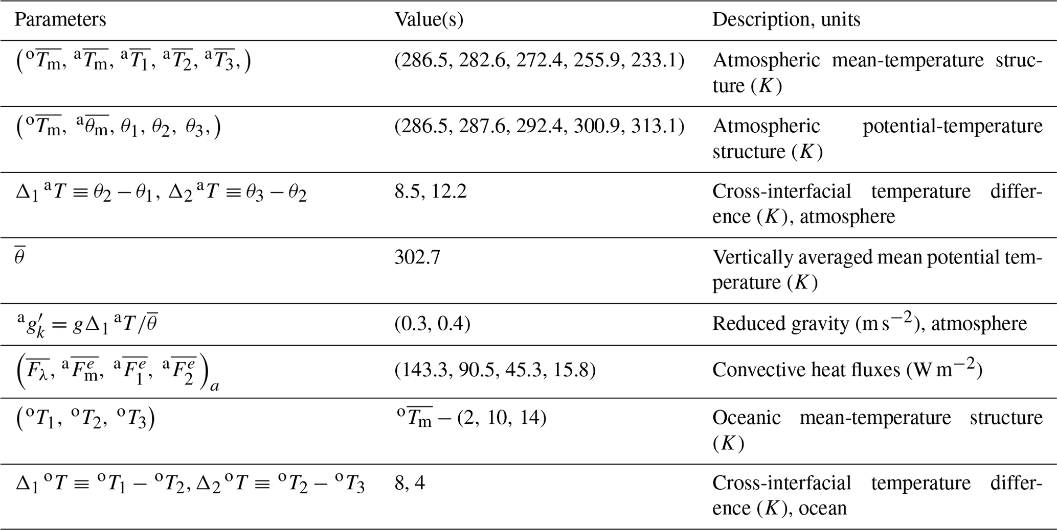
To solve for the mean state, we set all of $F_{\mathrm{m}}^{e+}$, ${}^{\mathrm{o}}{T}_{\mathrm{m}}^{\prime }$, ${}^{\mathrm{a}}{T}_{\mathrm{m}}^{\prime }$, ${}^{\mathrm{a}}{T}_{\mathrm{1}}^{\prime }$, ${}^{\mathrm{a}}{T}_{\mathrm{2}}^{\prime }$, and ${}^{\mathrm{a}}{T}_{\mathrm{3}}^{\prime }$ to zero and numerically integrate Eqs. (7)–(11) to equilibrium, using Euler differences in time with the time step of 5 min. Setting ${\mathit{\epsilon }}_{\mathrm{m}}={\mathit{\epsilon }}_{\mathrm{1}}={\mathit{\epsilon }}_{\mathrm{2}}={\mathit{\epsilon }}_{\mathrm{3}}=\mathrm{0.45}$ along with ${\stackrel{\mathrm{‾}}{F}}_{\mathrm{s}}=-\mathrm{240}$ W m⁻² results in the mean state whose parameters are listed in Table 1. The atmospheric optical depth decreases with altitude, but so do the unperturbed thicknesses of our chosen atmospheric layers, making the constant layer emissivities above a reasonable first approximation commensurate with an idealized nature of the present model. The model has a realistic (time-mean, global-mean) vertical temperature distribution. Note that the atmospheric reduced gravities are derived, in this version of the model, from the mean-state parameters rather than being prescribed (at 1.2 and 0.4 m s⁻²), as in the previous version (see the Appendix for further details). The climatological solution above is formally obtained over ocean, but it also applies over land of zero heat capacity (since the steady state does not depend on the heat capacity of the surface); the land's zero heat capacity is also a feature of the original Q-GCM formulation. The near-surface convective fluxes, however, would generally be different over ocean and over land (which occupies a significant fraction of the atmospheric channel, including fairly large strips both north and south of the ocean to avoid the distortion of ocean–atmosphere interaction by the effects associated with the atmospheric boundary conditions); the values of the convective fluxes in Table 1 should thus be interpreted to represent zonally averaged fluxes. Below, in Sect. 3.2, we will describe, among other things, modifications of the atmospheric-mixed-layer (AML) perturbation equation (that is, the one describing evolution of the anomalies with respect to the mean state) over land regions.

3.2 Mixed-layer perturbation equations and entrainment formulation

The perturbation equations in the mixed layers, for primed variables, have the same form as the first two Eqs. (7), aside from addition of advective and entrainment fluxes, which we will discuss further below; hereafter, we will drop primes in all perturbation equations for convenience. We will assume that the atmospheric perturbation temperature is vertically uniform, consistent with an active role of convection processes (cf. Manabe and Wetherald, 1967), namely

$$\begin{array}{}\text{(12)}& \begin{array}{rl}{}^{\mathrm{a}}{T}_{\mathrm{1}}^{\prime }& ={}^{\mathrm{a}}{T}_{\mathrm{2}}^{\prime }={}^{\mathrm{a}}{T}_{\mathrm{3}}^{\prime }\equiv {}^{\mathrm{a}}{T}^{\prime }=-({}^{\mathrm{a}}{\mathit{\eta }}_{\mathrm{1}}{\mathrm{\Delta }}_{\mathrm{1}}{}^{\mathrm{a}}T+{}^{\mathrm{a}}{\mathit{\eta }}_{\mathrm{2}}{\mathrm{\Delta }}_{\mathrm{2}}{}^{\mathrm{a}}T)/{}^{\mathrm{a}}H;\\ {}^{\mathrm{a}}H& \equiv {}^{\mathrm{a}}{H}_{\mathrm{1}}+{}^{\mathrm{a}}{H}_{\mathrm{2}}+{}^{\mathrm{a}}{H}_{\mathrm{3}},\end{array}\end{array}$$

(Δ_k ^aT above denotes the potential temperature jump across the kth interface; see Table 1), which allows one to express all perturbation radiative fluxes in Eq. (10) via perturbation oceanic and atmospheric-mixed-layer temperatures  ^oT_m and  ^aT_m and interfacial displacements  ^aη₁,  ^aη₂; in particular,

$$\begin{array}{}\text{(13)}& \begin{array}{rl}{F}_{\mathrm{0}}^{\uparrow }& =D_{\mathrm{0}}{}^{\mathrm{o}}{T}_{\mathrm{m}},\\ F_{\mathrm{m}}^{\uparrow }& =D_{\mathrm{m}}^{\uparrow }{}^{\mathrm{a}}{T}_{\mathrm{m}}+E_{\mathrm{0}}^{\uparrow }{}^{\mathrm{o}}{T}_{\mathrm{m}},\\ F_{\mathrm{1}}^{\uparrow }& =A_{\mathrm{1},\mathrm{1}}^{\uparrow }{}^{\mathrm{a}}{\mathit{\eta }}_{\mathrm{1}+}{A}_{\mathrm{1},\mathrm{2}}^{\uparrow }{}^{\mathrm{a}}{\mathit{\eta }}_{\mathrm{2}+}{D}_{\mathrm{1}}^{\uparrow }{}^{\mathrm{a}}{T}_{\mathrm{m}}+E_{\mathrm{1}}^{\uparrow }{}^{\mathrm{o}}{T}_{\mathrm{m}},\\ F_{\mathrm{2}}^{\uparrow }& =A_{\mathrm{2},\mathrm{1}}^{\uparrow }{}^{\mathrm{a}}{\mathit{\eta }}_{\mathrm{1}+}{A}_{\mathrm{2},\mathrm{2}}^{\uparrow }{}^{\mathrm{a}}{\mathit{\eta }}_{\mathrm{2}+}{D}_{\mathrm{2}}^{\uparrow }{}^{\mathrm{a}}{T}_{\mathrm{m}}+E_{\mathrm{2}}^{\uparrow }{}^{\mathrm{o}}{T}_{\mathrm{m}},\\ F_{\mathrm{3}}^{\uparrow }& =A_{\mathrm{3},\mathrm{1}}^{\uparrow }{}^{\mathrm{a}}{\mathit{\eta }}_{\mathrm{1}+}{A}_{\mathrm{3},\mathrm{2}}^{\uparrow }{}^{\mathrm{a}}{\mathit{\eta }}_{\mathrm{2}+}{D}_{\mathrm{3}}^{\uparrow }{}^{\mathrm{a}}{T}_{\mathrm{m}}+E_{\mathrm{3}}^{\uparrow }{}^{\mathrm{o}}{T}_{\mathrm{m}},\\ F_{\mathrm{3}}^{\downarrow }& =A_{\mathrm{3},\mathrm{1}}^{\downarrow }{}^{\mathrm{a}}{\mathit{\eta }}_{\mathrm{1}}+A_{\mathrm{3},\mathrm{2}}^{\downarrow }{}^{\mathrm{a}}{\mathit{\eta }}_{\mathrm{2}},\\ F_{\mathrm{2}}^{\downarrow }& =A_{\mathrm{2},\mathrm{1}}^{\downarrow }{}^{\mathrm{a}}{\mathit{\eta }}_{\mathrm{1}}+A_{\mathrm{2},\mathrm{2}}^{\downarrow }{}^{\mathrm{a}}{\mathit{\eta }}_{\mathrm{2}},\\ F_{\mathrm{1}}^{\downarrow }& =A_{\mathrm{1},\mathrm{1}}^{\downarrow }{}^{\mathrm{a}}{\mathit{\eta }}_{\mathrm{1}}+A_{\mathrm{1},\mathrm{2}}^{\downarrow }{}^{\mathrm{a}}{\mathit{\eta }}_{\mathrm{2}},\\ F_{\mathrm{m}}^{\downarrow }& =F_{\mathrm{1}}^{\downarrow }\left(\mathrm{1}-{\mathit{\epsilon }}_{\mathrm{m}}\right)+D_{\mathrm{m}}^{\downarrow {}^{\mathrm{a}}}{T}_{\mathrm{m}},\end{array}\end{array}$$

where the A, D, and E coefficients can be written in terms of the known mean-state parameters. The Eq. (13) above should be compared with Eqs. (4.2)–(4.6) of the Q-GCM user's guide (Hogg et al., 2014). Notably, the parameter ε_m was effectively set to 1 in the previous version of Q-GCM, and hence the E coefficients were equal to zero. On the other hand, that previous version had additional parameters B and C for radiative corrections associated with the variable AML depth and topography. Here we are back to the model with a constant AML depth (see below); we also neglect topography corrections for simplicity.

Another consequence of the assumption ε_m<1, used here, is that the coefficients A, D, and E in Eq. (13) over ocean and over land are different, and so is the AML temperature equation – the second equation in Eq. (7). In particular, over land, we have (neglecting, for now, advection and entrainment terms in the AML equation)

$$\begin{array}{}\text{(14)}& \begin{array}{rl}& \mathrm{0}=-F_l^{\uparrow }-F_{\mathrm{m}}^{\downarrow }-F_{\mathrm{s}},\\ & {}^{\mathrm{a}}\mathit{\rho }{}^{\mathrm{a}}{C}_p{}^{\mathrm{a}}{H}_{\mathrm{m}}{}^{\mathrm{a}}{\dot{T}}_{\mathrm{m}}=F_l^{\uparrow }+F_{\mathrm{m}}^{\downarrow }-\left(F_{\mathrm{m}}^{\uparrow }+{}^{\mathrm{a}}{F}_{\mathrm{m}}^{e-}+F_{\mathrm{1}}^{\downarrow }\right),\end{array}\end{array}$$

where $F_l^{\uparrow }$ is the infrared upward flux from the surface of the land, with the latter assumed to have zero heat capacity (hence zero on the left-hand side of the first equation in Eq. 14) and conductivity (hence F_λ=0). From Eq. (14) it follows that over land

$$\begin{array}{}\text{(15)}& \begin{array}{rl}& F_l^{\uparrow }=-F_{\mathrm{m}}^{\downarrow }-F_{\mathrm{s}},\\ & {}^{\mathrm{a}}\mathit{\rho }{}^{\mathrm{a}}{C}_p{}^{\mathrm{a}}{H}_{\mathrm{m}}{}^{\mathrm{a}}{\dot{T}}_{\mathrm{m}}=-F_{\mathrm{s}}-\left(F_{\mathrm{m}}^{\uparrow }+{}^{\mathrm{a}}{F}_{\mathrm{m}}^{e-}+F_{\mathrm{1}}^{\downarrow }\right),\end{array}\end{array}$$

while, in analogy with Eq. (10),

$$\begin{array}{}\text{(16)}& \begin{array}{rl}{F}_{\mathrm{m}}^{\uparrow }& =F_l^{\uparrow }\left(\mathrm{1}-{\mathit{\epsilon }}_{\mathrm{m}}\right)+D_{\mathrm{m}}^{\uparrow }{}^{\mathrm{a}}{T}_{\mathrm{m}}\\ & =-\left(F_{\mathrm{m}}^{\downarrow }+F_{\mathrm{s}}\right)\left(\mathrm{1}-{\mathit{\epsilon }}_{\mathrm{m}}\right)+D_{\mathrm{m}}^{\uparrow {}^{\mathrm{a}}}{T}_{\mathrm{m}}\end{array}\end{array}$$

(compare this with the second Eq. 13). The first (additional) term in Eq. (16) will also modify all other upwelling radiation fluxes ($F_{\mathrm{1}}^{\uparrow },F_{\mathrm{2}}^{\uparrow },F_{\mathrm{3}}^{\uparrow })$ accordingly through Eq. (10), resulting in modified values of the A and D coefficients and all E coefficients set to zero over land.

Yet another, minor, but potentially fairly important modification of the previous Q-GCM formulation is the inclusion of the dependence on the relative wind speed | ^au_m− ^ou_m| in the bulk formulas for the sensible/latent-heat ocean–atmosphere exchange, which plays a significant role in setting up the North Atlantic SST tripole variability (Deser and Blackmon, 1993; Kushnir, 1994; Czaja and Marshall, 2001; Kravtsov et al., 2007; Fan and Schneider, 2012):

$$\begin{array}{}\text{(17)}& F_{\mathit{\lambda }}=(\mathit{\lambda }+{}^{\mathrm{a}}\mathit{\rho }{}^{\mathrm{a}}{C}_p{C}_{\mathrm{h}}\left|{}^{\mathrm{a}}{\mathbf{u}}_{\mathrm{m}}-\left.{}^{\mathrm{o}}{\mathbf{u}}_{\mathrm{m}}\right|\right.)({}^{\mathrm{o}}{T}_{\mathrm{m}}-{}^{\mathrm{a}}{T}_{\mathrm{m}})\end{array}$$

(compare with Eqs. 4.7–4.9 in Hogg et al., 2014), where we use the values of λ=5 W m⁻² K⁻¹ and C_h=0.004; with the typical relative wind speed of $\left|{}^{\mathrm{a}}{\mathbf{u}}_{\mathrm{m}}-\left.{}^{\mathrm{o}}{\mathbf{u}}_{\mathrm{m}}\right|\right.\approx \mathrm{7.5}$ m s⁻¹, the magnitude of the total sensible/latent-heat exchange coefficient in Eq. (17) would be equal to 35 W m⁻² K⁻¹, which is the value of λ used in the previous edition of Q-GCM (Hogg et al., 2014), along with the value of C_h=0.

To complete the mixed-layer heat conservation equations, we need to add advection, diffusion, and entrainment heat fluxes, namely

$$\begin{array}{}\text{(18)}& \begin{array}{rl}{}^{\mathrm{o}}{T}_{\mathrm{m}t}& +({}^{\mathrm{o}}{u}_{\mathrm{m}}{}^{\mathrm{o}}{T}_{\mathrm{m}}{)}_x+({}^{\mathrm{o}}{v}_{\mathrm{m}}{}^{\mathrm{o}}{T}_{\mathrm{m}}{)}_y-{\displaystyle \frac{{}^{\mathrm{o}}{w}_{\mathrm{ek}}{}^{\mathrm{o}}{T}_{\mathrm{m}}}{{}^{\mathrm{o}}{H}_{\mathrm{m}}}}\\ & ={}^{\mathrm{o}}{K}_{\mathrm{2}}{\mathrm{\nabla }}_H^{\mathrm{2}}{}^{\mathrm{o}}{T}_{\mathrm{m}}-{}^{\mathrm{o}}{K}_{\mathrm{4}}{\mathrm{\nabla }}_H^{\mathrm{4}}{}^{\mathrm{o}}{T}_{\mathrm{m}}\\ & +{\displaystyle \frac{\mathrm{1}}{{}^{\mathrm{o}}\mathit{\rho }{}^{\mathrm{o}}{C}_p{}^{\mathrm{o}}{H}_{\mathrm{m}}}}\left(-F_{\mathit{\lambda }}-F_{\mathrm{0}}^{\uparrow }-F_{\mathrm{m}}^{\downarrow }-F_{\mathrm{s}}+{}^{\mathrm{o}}{F}_{\mathrm{m}}^{e+}\right),\\ {}^{\mathrm{a}}{T}_{\mathrm{m}t}& +({}^{\mathrm{a}}{u}_{\mathrm{m}}{}^{\mathrm{a}}{T}_{\mathrm{m}}{)}_x\\ & +({}^{\mathrm{a}}{v}_{\mathrm{m}}{}^{\mathrm{a}}{T}_{\mathrm{m}}{)}_y+{\displaystyle \frac{{}^{\mathrm{a}}{w}_{\mathrm{ek}}{}^{\mathrm{a}}{T}_{\mathrm{m}}}{{}^{\mathrm{a}}{H}_{\mathrm{m}}}}={}^{\mathrm{a}}{K}_{\mathrm{2}}{\mathrm{\nabla }}_H^{\mathrm{2}}{}^{\mathrm{a}}{T}_{\mathrm{m}}-{}^{\mathrm{a}}{K}_{\mathrm{4}}{\mathrm{\nabla }}_H^{\mathrm{4}}{}^{\mathrm{a}}{T}_{\mathrm{m}}\\ & +{\displaystyle \frac{\mathrm{1}}{{}^{\mathrm{a}}\mathit{\rho }{}^{\mathrm{a}}{C}_p{}^{\mathrm{a}}{H}_{\mathrm{m}}}}\left(F_{\mathit{\lambda }}+F_{\mathrm{0}}^{\uparrow }+F_{\mathrm{m}}^{\downarrow }-(F_{\mathrm{m}}^{\uparrow }+{}^{\mathrm{a}}{F}_{\mathrm{m}}^{e-}+F_{\mathrm{1}}^{\downarrow })\right);\end{array}\end{array}$$

compare this with the first two Eqs. (7) and with Eqs. (3.28)–(29) in Hogg et al. (2014); the biharmonic viscosity term on the right-hand side is included mainly for numerical stability. As mentioned above, in contrast to the previous Q-GCM formulation, we use here the constant mixed-layer thickness in both the ocean and the atmosphere. Therefore, in both the ocean and the atmosphere, entrainment is solely driven by the Ekman pumping. Neglecting vertical diffusion and convection in the present perturbation model (which is another difference from Hogg et al., 2014), we write for the ocean, following McDougall and Dewar (1998) and Kravtsov et al. (2007),

$$\begin{array}{}\text{(19)}& \begin{array}{rl}& {}^{\mathrm{o}}{F}_{\mathrm{m}}^{e+}={}^{\mathrm{o}}\mathit{\rho }{}^{\mathrm{o}}{C}_p{}^{\mathrm{o}}{w}_{\mathrm{ek}}\left({}^{\mathrm{o}}{T}_{\mathrm{1}}-{}^{\mathrm{o}}{T}_{\mathrm{m}}\right),{}^{\mathrm{o}}{F}_{\mathrm{m}}^{e-}=\mathrm{0},\mathrm{if}{}^{\mathrm{o}}{w}_{\mathrm{ek}}>\mathrm{0}\\ & {}^{\mathrm{o}}{F}_{\mathrm{m}}^{e+}=\mathrm{0},{}^{\mathrm{o}}{F}_{\mathrm{m}}^{e-}=-{}^{\mathrm{o}}\mathit{\rho }{}^{\mathrm{o}}{C}_p{}^{\mathrm{o}}{w}_{\mathrm{ek}}\left({}^{\mathrm{o}}{T}_{\mathrm{1}}-{}^{\mathrm{o}}{T}_{\mathrm{m}}\right),\mathrm{otherwise};\end{array}\end{array}$$

cf. Eqs. (4.30)–(31) of Hogg et al. (2014). The entrainment in the ocean interior only occurs between layers 1 and 2 and is computed in the same way as in the original model:

$$\begin{array}{}\text{(20)}& {}^{\mathrm{o}}{e}_{\mathrm{1}}={\displaystyle \frac{{}^{\mathrm{o}}{F}_{\mathrm{m}}^{e-}}{{\mathrm{\Delta }}_{\mathrm{1}}{}^{\mathrm{o}}T}}\end{array}$$

(Hogg et al., 2014, Eq. 4.32); following, again, Hogg et al. (2014),  ^oe₁ is also corrected to have a zero area integral by adding a spatially uniform offset value at each time step.

Similarly, in the atmospheric mixed layer

$$\begin{array}{}\text{(21)}& \begin{array}{rl}& {}^{\mathrm{a}}{F}_{\mathrm{m}}^{e+}={}^{\mathrm{a}}\mathit{\rho }{}^{\mathrm{a}}{C}_p{}^{\mathrm{a}}{w}_{\mathrm{ek}}\left({}^{\mathrm{a}}{T}_{\mathrm{m}}-{}^{\mathrm{a}}{T}_{\mathrm{1}}\right),{}^{\mathrm{a}}{F}_{\mathrm{m}}^{e-}=\mathrm{0},\mathrm{if}{}^{\mathrm{a}}{w}_{\mathrm{ek}}>\mathrm{0}\\ & {}^{\mathrm{a}}{F}_{\mathrm{m}}^{e+}=\mathrm{0},{}^{\mathrm{a}}{F}_{\mathrm{m}}^{e-}=-{}^{\mathrm{a}}\mathit{\rho }{}^{\mathrm{a}}{C}_p{}^{\mathrm{a}}{w}_{\mathrm{ek}}\left({}^{\mathrm{a}}{T}_{\mathrm{m}}-{}^{\mathrm{a}}{T}_{\mathrm{1}}\right),\mathrm{otherwise}.\end{array}\end{array}$$

Here  ^aT₁ is the perturbation temperature given by Eq. (12); in the mean state this temperature is set to ${}^{\mathrm{a}}\stackrel{\mathrm{‾}}{T_{\mathrm{m}}}$. Using  ^aT₁ instead of θ₁ in Eqs. (19) is what keeps the instability described by Hogg et al. (2003) in check in the present version of the model with constant  ^aH_m. This is due to the fact that  ^aT₁ is tied to the instantaneous vertical structure of the atmosphere, which limits the magnitude of entrainment heat fluxes (as  ^aT₁ tends to be closer to  ^aT_m than θ₁) and also provides additional negative feedbacks in the quasi-geostrophic potential vorticity (QGPV) equations via the dependence of entrainment fluxes on η.

Finally, a major modification in the present version of the Q-GCM model is the formulation of entrainment fluxes in the interior of the atmosphere. In the previous version of the model, all entrainment was assumed to occur at the lowest interface, leading to unrealistically small vertical shears of horizontal velocity in the upper atmosphere. Here we correct this by allowing the thermal forcing of the upper troposphere and entrainment through both atmospheric interfaces. The perturbation heat conservation equations for the interior atmospheric layers can be obtained by setting the time derivatives on the left-hand side of the last three Eqs. (7) to zero and using the jump conditions (McDougall and Dewar, 1998) at the interfaces:

$$\begin{array}{}\text{(22)}& \begin{array}{rl}& \mathrm{0}=F_{\mathrm{m}}^{\uparrow }+F_{\mathrm{1}}^{\downarrow }+{}^{\mathrm{a}}{F}_{\mathrm{m}}^{e+}-\left(F_{\mathrm{1}}^{\uparrow }+F_{\mathrm{2}}^{\downarrow }+{}^{\mathrm{a}}{F}_{\mathrm{1}}^{e-}\right),\\ & \mathrm{0}=F_{\mathrm{1}}^{\uparrow }+F_{\mathrm{2}}^{\downarrow }+{}^{\mathrm{a}}{F}_{\mathrm{1}}^{e+}-\left(F_{\mathrm{2}}^{\uparrow }+F_{\mathrm{3}}^{\downarrow }+{}^{\mathrm{a}}{F}_{\mathrm{2}}^{e-}\right),\\ & \mathrm{0}=F_{\mathrm{2}}^{\uparrow }+F_{\mathrm{3}}^{\downarrow }+{}^{\mathrm{a}}{F}_{\mathrm{2}}^{e+}-F_{\mathrm{3}}^{\uparrow },\\ & {}^{\mathrm{a}}{F}_k^{e+}-{}^{\mathrm{a}}{F}_k^{e-}=-{}^{\mathrm{a}}\mathit{\rho }{}^{\mathrm{a}}{C}_p{}^{\mathrm{a}}{e}_k{\mathrm{\Delta }}_k{}^{\mathrm{a}}T;k=\mathrm{1},\mathrm{2}\end{array}\end{array}$$

(compare this with Eqs. 4.10–4.12 of the Q-GCM user's guide; Hogg et al., 2014). Adding up the first three Eqs. (22) and using the fourth equation for the jump conditions allows one to write

$$\begin{array}{}\text{(23)}& \mathit{\rho }{}^{\mathrm{a}}{C}_p\left({}^{\mathrm{a}}{e}_{\mathrm{1}}{\mathrm{\Delta }}_{\mathrm{1}}{}^{\mathrm{a}}T+{}^{\mathrm{a}}{e}_{\mathrm{2}}{\mathrm{\Delta }}_{\mathrm{2}}{}^{\mathrm{a}}T\right)=F_{\mathrm{m}}^{\uparrow }+F_{\mathrm{1}}^{\downarrow }+{}^{\mathrm{a}}{F}_{\mathrm{m}}^{e+}-F_{\mathrm{3}}^{\uparrow }.\end{array}$$

Hogg et al. (2014) assumed  ^ae₂=0. We modify this assumption by making the entrainments across the lower and upper atmospheric interface be linearly related, with the coefficient f₂ (see below); this procedure can also be adapted for the use in an n-layer model by introducing additional free parameters analogous to f₂. To allow 1 degree of freedom in controlling damping rates at each interface somewhat independently, we also introduce here a (small) vertical diffusion, using a linearized version of the McDougall and Dewar (1998) formulation:

$$\begin{array}{}\text{(24)}& \begin{array}{rl}{}^{\mathrm{a}}{e}_{\mathrm{1}}& ={}^{\mathrm{a}}{e}_{\mathrm{1}}^{\prime }+{\mathit{\mu }}_{\mathrm{1}}^{\ast }\left({\displaystyle \frac{\mathrm{1}}{{}^{\mathrm{a}}{H}_{\mathrm{1}}}}+{\displaystyle \frac{\mathrm{1}}{{}^{\mathrm{a}}{H}_{\mathrm{2}}}}\right){}^{\mathrm{a}}{\mathit{\eta }}_{\mathrm{1}}-{\displaystyle \frac{{\mathit{\mu }}_{\mathrm{1}}^{\ast }}{{}^{\mathrm{a}}{H}_{\mathrm{2}}}}{}^{\mathrm{a}}{\mathit{\eta }}_{\mathrm{2}},\\ {}^{\mathrm{a}}{e}_{\mathrm{2}}& ={}^{\mathrm{a}}{e}_{\mathrm{2}}^{\prime }+{\mathit{\mu }}_{\mathrm{2}}^{\ast }\left({\displaystyle \frac{\mathrm{1}}{{}^{\mathrm{a}}{H}_{\mathrm{2}}}}+{\displaystyle \frac{\mathrm{1}}{{}^{\mathrm{a}}{H}_{\mathrm{3}}}}\right){}^{\mathrm{a}}{\mathit{\eta }}_{\mathrm{2}}-{\displaystyle \frac{{\mathit{\mu }}_{\mathrm{2}}^{\ast }}{{}^{\mathrm{a}}{H}_{\mathrm{2}}}}{}^{\mathrm{a}}{\mathit{\eta }}_{\mathrm{1}},\\ {}^{\mathrm{a}}{e}_{\mathrm{2}}^{\prime }& =f_{\mathrm{2}}{}^{\mathrm{a}}{e}_{\mathrm{1}}^{\prime }.\end{array}\end{array}$$

We can now solve the system (23)–(24) for the two unknown non-diffusive entrainment rates ${}^{\mathrm{a}}{e}_{\mathrm{1}}^{\prime }$ and ${}^{\mathrm{a}}{e}_{\mathrm{2}}^{\prime }$ and, hence, for the full entrainment rates  ^ae₁ and  ^ae₂. We use the nominal value of 0.0001 m s⁻¹ for both of ${\mathit{\mu }}_{\mathrm{1}}^{\ast }$ and ${\mathit{\mu }}_{\mathrm{2}}^{\ast }$ and initially set

$$\begin{array}{}\text{(25)}& f_{\mathrm{2}}={\displaystyle \frac{{}^{\mathrm{a}}{g}_{\mathrm{1}}^{\prime }}{{}^{\mathrm{a}}{g}_{\mathrm{2}}^{\prime }}}\end{array}$$

to ensure generation of similar velocity shears between atmospheric layers $\mathrm{1}/\mathrm{2}$ and $\mathrm{2}/\mathrm{3}$ by the thermal forcing of a given amplitude. Increasing f₂ would tend to increase the geostrophic zonal velocity shear between the lower two atmospheric layers and decrease the velocity shear between the upper two atmospheric layers; setting f₂=0 recovers the previous Q-GCM formulation. The optimal value of f₂ is to be determined by trial-and-error tuning of the model.

3.3 Temperature-dependent flow in the atmospheric mixed layer and partially coupled setup

We introduce temperature dependence of the AML winds by modifying the mixed-layer momentum equations in two ways, namely (i) including, explicitly, temperature-driven pressure gradients (which takes into account the mixed-layer hydrostatic adjustment to temperature contrasts: Lindzen and Nigam, 1987), following Feliks et al. (2004, 2007, 2011); and (ii) making the surface drag coefficient depend on the ocean–atmosphere temperature difference to parameterize changes in AML stability (Wallace et al., 1989), following Hogg et al. (2009); see Small et al. (2008) and Chelton and Xie (2010) for a review of these two mechanisms for mesoscale air–sea coupling. Putrasahan et al. (2013) demonstrated that, in the Kuroshio region, both mechanisms (i) and (ii) are important, with relative contributions depending on the spatial scale of the SST anomalies. Putrasahan et al. (2017) also concluded that heat advection by oceanic mesoscale currents plays a key role in creating such SST anomalies and forcing the MABL response in the Gulf of Mexico. To implement these changes, we write the AML momentum equations as

$$\begin{array}{}\text{(26)}& \begin{array}{rl}& {}^{\mathrm{a}}{u}_{\mathrm{m}}={}^{\mathrm{a}}{u}_{\mathrm{1}}+{\mathit{\alpha }}_T{\displaystyle \frac{\mathrm{1}}{\mathrm{2}}}{\displaystyle \frac{g{}^{\mathrm{a}}{H}_{\mathrm{m}}}{{\mathit{\theta }}_{\mathrm{0}}{f}_{\mathrm{0}}}}{\displaystyle \frac{\partial {}^{\mathrm{a}}{T}_{\mathrm{m}}}{\partial y}}-{\displaystyle \frac{{}^{\mathrm{a}}{\mathit{\tau }}^y}{{}^{\mathrm{a}}{H}_{\mathrm{m}}{f}_{\mathrm{0}}}},\\ & {}^{\mathrm{a}}{v}_{\mathrm{m}}={}^{\mathrm{a}}{v}_{\mathrm{1}}-{\mathit{\alpha }}_T{\displaystyle \frac{\mathrm{1}}{\mathrm{2}}}{\displaystyle \frac{g{}^{\mathrm{a}}{H}_{\mathrm{m}}}{{\mathit{\theta }}_{\mathrm{0}}{f}_{\mathrm{0}}}}{\displaystyle \frac{\partial {}^{\mathrm{a}}{T}_{\mathrm{m}}}{\partial x}}+{\displaystyle \frac{{}^{\mathrm{a}}{\mathit{\tau }}^x}{{}^{\mathrm{a}}{H}_{\mathrm{m}}{f}_{\mathrm{0}}}},\\ & \left({}^{\mathrm{a}}{\mathit{\tau }}^x,{}^{\mathrm{a}}{\mathit{\tau }}^y\right)=C_D\max (\mathrm{1}+\mathit{\alpha }\mathrm{\Delta }T,\mathrm{0.1})\left|{}^{\mathrm{a}}{\mathbf{u}}_{\mathrm{m}}-{}^{\mathrm{o}}{\mathbf{u}}_{\mathrm{m}}\right|\\ & \left({}^{\mathrm{a}}{u}_{\mathrm{m}}-{}^{\mathrm{o}}{u}_{\mathrm{m},}{}^{\mathrm{a}}{v}_{\mathrm{m}}-{}^{\mathrm{o}}{v}_{\mathrm{m}}\right),\end{array}\end{array}$$

where ( ^au₁,  ^av₁) is the geostrophic velocity in the lowest atmospheric layer, ( ^aτ^x, ^aτ^y) is the wind stress, $\mathrm{\Delta }T={}^{\mathrm{o}}{T}_{\mathrm{m}}-{}^{\mathrm{a}}{T}_{\mathrm{m}}$, α_T=1, and α=0.15. Setting one of the α parameters to zero can be used to examine processes (i) and (ii) above independently; setting both of these parameters to zero would recover the previous, temperature-independent AML wind formulation (3.2)–(3.3) of Hogg et al. (2014). On top of these modifications, we also set the drag coefficient over ocean to two-thirds of the default value over land, following Marshall and Molteni (1993).

Upon adding to Eq. (26) analogous equations for the oceanic mixed layer in their original form (Hogg et al., 2014; Eqs. 3.4–3.5), we end up with a closed system of equations for the unknown values of ( ^aτ^x, ^aτ^y) at each grid point, which can be solved analytically in the same way as before (see Hogg et al., 2014). Note that additional temperature gradients in the first two Eqs. (26) produce a non-divergent wind field with zero direct Ekman pumping and, also, zero temperature advection contributions; their dynamical effect is thus purely indirect, via modifications to the wind-stress field; they also generate non-zero moisture advection in the moist version of the Q-GCM model, to be developed later in Sect. 4.

The temperature-dependent AML wind formulation (26) is associated with coupled feedbacks that tend to suppress oceanic turbulence and SST fronts (cf. Hogg et al., 2014; see also Sect. 5). In principle, a realistic mesoscale ocean field can still be achieved in inherently more turbulent oceanic regimes at high Reynolds numbers, but this requires very high ocean resolution and is computationally demanding. An alternative fix is to apply partial momentum coupling of the oceanic and atmospheric mixed layers, in which the atmosphere “sees” the wind stress as per the full version of Eq. (26), whereas the oceanic wind stress is computed from Eq. (26), in which ${\mathit{\alpha }}_T=\mathit{\alpha }=\mathrm{0}$. In this way the mesoscale feedbacks of temperature-dependent wind, which damp oceanic turbulence, are artificially suppressed, but their effect on the atmosphere is preserved, possibly leading to coupled dynamics involving large-scale low-frequency reorganization of the wind field and the ensuing ocean response.

3.4 Lateral boundary conditions for mass and temperature equations

The original Q-GCM formulation employed no-through-flow conditions on the zonal boundaries of the atmospheric channel but effectively allowed the mass to leave/enter ocean mixed layer through side boundaries to avoid Ekman pumping singularities there (via the direct use of Eqs. 3.5 and 3.18 to compute the oceanic Ekman pumping in Hogg et al., 2014); this means, among other things, that the area integral of Ekman pumping over the ocean basin does not vanish. Although it is a lesser problem in the atmospheric setup, we modify the computation of the atmospheric Ekman pumping at the zonal boundaries accordingly to achieve a uniform model formulation and to avoid an abnormal boundary pumping in the atmosphere. To do so, instead of setting  ^av_m to zero at the zonal boundaries, we assign it the values computed by the second Eq. (26), with the Ekman pumping computed as usual – in terms of the divergence of the mixed-layer horizontal velocity field – by Eq. (3.16) or, equivalently, via curl of the wind stress by Eq. (3.17) in Hogg et al. (2014).

Naturally, with open boundaries in both the ocean and the atmosphere, we also let the fluid leaving/entering the basin to have temperature determined by the Neumann boundary condition of zero temperature derivative in the direction normal to the boundary:

$$\begin{array}{}\text{(27)}& {\displaystyle \frac{\partial T_{\mathrm{m}}}{\partial n}}=\mathrm{0},\end{array}$$

where T_m denotes either atmospheric or oceanic-mixed-layer temperature. With the open boundary condition augmented by Eq. (27), it is no longer necessary to specify the temperature at the ocean's equatorward boundary, as was done in Hogg et al. (2014).

4 Moist version of the model: MQ-GCM

Perhaps the most important change to the original Q-GCM formulation is the inclusion of the hydrological cycle and latent-heat feedbacks, resulting in what we refer to as the Moist Quasi-Geostrophic Coupled Model (MQ-GCM). Indeed, Czaja and Blunt (2011) proposed that the oceans can influence the troposphere through moist convection over the regions with strong mesoscale variability; see also Willison et al. (2013). To compute moisture variables in the model, we assume that the vertical temperature profile at a given (x, y) location is linear in z, with temperature decreasing with altitude z above the sea level at the critical lapse rate γ_c:

$$\begin{array}{}\text{(28)}& T_k\left(z\right)={}^{\mathrm{a}}\stackrel{\mathrm{‾}}{T_{\mathrm{m}}}-\left({\mathrm{\Gamma }}_{\mathrm{d}}-{\mathit{\gamma }}_{\mathrm{c}}\right){\displaystyle \frac{{}^{\mathrm{a}}{H}_{\mathrm{m}}}{\mathrm{2}}}+{}^{\mathrm{a}}{T}_k-{\mathit{\gamma }}_{\mathrm{c}}z.\end{array}$$

Here T_k is the absolute temperature (in K) in layer k (k can be a symbol (m) when referring to the AML temperature or an index (k=1, 2, 3) when denoting the interior (quasi-geostrophic) layers of the atmospheric model), while  ^aT_k in the interior is given by Eq. (12). In such a constant-lapse-rate atmosphere, the pressure p(z) is related to temperature as

$$\begin{array}{}\text{(29)}& p\left(z\right)=p_{\mathrm{0}}{\left({\displaystyle \frac{T\left(z\right)}{T\left(\mathrm{0}\right)}}\right)}^{\frac{g}{R{\mathit{\gamma }}_{\mathrm{c}}}},\end{array}$$

where g is the gravity acceleration and R is the ideal gas constant for dry air. Combining the latter two equations and the ideal gas law p=ρRT at the basic state with  ^aT_k=0, we can compute the representative densities of each layer by estimating them at the altitude z, corresponding to the mid-layer height ($z={}^{\mathrm{a}}{H}_{\mathrm{m}}/\mathrm{2}$ for the mixed layer, $z={}^{\mathrm{a}}{H}_{\mathrm{m}}+{}^{\mathrm{a}}{H}_{\mathrm{1}}/\mathrm{2}$ for layer 1, etc.); this gives, for the parameters in Table 1 and p₀=10⁵ hPa, $\left({\mathit{\rho }}_{\mathrm{m}},{\mathit{\rho }}_{\mathrm{1}},{\mathit{\rho }}_{\mathrm{2}},{\mathit{\rho }}_{\mathrm{3}}\right)=\left(\mathrm{1.16},\mathrm{1},\mathrm{0.77},\mathrm{0.52}\right)$ kg m⁻³. The saturation specific humidity h_s is given by

$$\begin{array}{}\text{(30)}& h_{\mathrm{s}}=\mathit{\epsilon }{\displaystyle \frac{e_{\mathrm{s}}}{p}};e_{\mathrm{s}}=e_o\exp \left({\displaystyle \frac{a\left(T-T_{\mathrm{0}}\right)}{b\left(T-T_{\mathrm{0}}\right)+T_r}}\right),\end{array}$$

where $\mathit{\epsilon }=R/R_{\mathrm{v}}=\mathrm{0.62}$ is the ratio of the dry-air and water vapor gas constants, and the saturation water vapor pressure e_s is computed as in Bolton (1980), using the parameters e₀=611.2 hPa, a=17.67, b=1, T_r=243.5 K, and T₀=273.15 K. Given the AML perturbation temperature  ^aT_m and the atmospheric interface displacements  ^aη₁,  ^aη₂, the Eqs. (12) and (28)–(30) can be used to compute the saturation specific humidity as a function of z at every grid point (x, y) and within each atmospheric layer $k=\left(m,\mathrm{1},\mathrm{2},\mathrm{3}\right)$

The moist version of the Q-GCM model has, compared with the original dry model, additional variables representing the specific humidity $h_k(x,y,t)$ in each layer; these variables are discretized on the model's T grid. The specific humidity is assumed to be independent of z except when used in the formulas parameterizing moisture fluxes at the top and bottom of the AML (see below). The humidity equations in both the AML and the atmospheric interior are largely analogous to the AML temperature Eq. (18) (cf. Deremble et al., 2013) and are given by

$$\begin{array}{}\text{(31)}& \begin{array}{rl}{h}_{\mathrm{m}t}& +({}^{\mathrm{a}}{u}_{\mathrm{m}}{h}_{\mathrm{m}}{)}_x+({}^{\mathrm{a}}{v}_{\mathrm{m}}{h}_{\mathrm{m}}{)}_y+{\displaystyle \frac{{}^{\mathrm{a}}{w}_{\mathrm{ek}}{h}_{\mathrm{m}}}{{}^{\mathrm{a}}{H}_{\mathrm{m}}}}\\ & ={}^{\mathrm{a}}{K}_{\mathrm{2}}{\mathrm{\nabla }}_H^{\mathrm{2}}{h}_{\mathrm{m}}-{}^{\mathrm{a}}{K}_{\mathrm{4}}{\mathrm{\nabla }}_H^{\mathrm{4}}{h}_{\mathrm{m}}\\ & +{\displaystyle \frac{\mathrm{1}}{{\mathit{\rho }}_{\mathrm{m}}{}^{\mathrm{a}}{H}_{\mathrm{m}}}}\left(E-P_{\mathrm{m}}-F_{\mathrm{m}}^{e-}\right);\\ h_{kt}& +({}^{\mathrm{a}}{u}_k^{\mathrm{g}}{h}_k{)}_x+({}^{\mathrm{a}}{v}_k^{\mathrm{g}}{h}_k{)}_y\\ & ={}^{\mathrm{a}}{K}_{\mathrm{2}}{\mathrm{\nabla }}_H^{\mathrm{2}}{h}_k-{}^{\mathrm{a}}{K}_{\mathrm{4}}{\mathrm{\nabla }}_H^{\mathrm{4}}{h}_k\\ & +{\displaystyle \frac{\mathrm{1}}{{\mathit{\rho }}_k{}^{\mathrm{a}}{H}_k}}\left(F_{k-\mathrm{1}}^{e+}-P_k-F_k^{e-}\right).\end{array}\end{array}$$

Here $\left({}^{\mathrm{a}}{u}_k^{\mathrm{g}},{}^{\mathrm{a}}{v}_k^{\mathrm{g}}\right)$ are the geostrophic velocities in the atmospheric layer k, E is the evaporation, and P_k is the precipitation; $F_k^{e-}$ and $F_k^{e+}$ are the moisture entrainment fluxes below and above the interface k, respectively (all of these fluxes are in kg m⁻² s⁻¹). Once again, $k=(m,\mathrm{1},\mathrm{2},\mathrm{3})$ and $k-\mathrm{1}\to m$ for k=1. The biharmonic viscosity term on the right-hand side is, again, included mainly for numerical stability. The Eq. (31) also uses boundary conditions analogous to those for temperature (Sect. 3.4).

The evaporation over the ocean is given by (Gill, 1982)

$$\begin{array}{}\text{(32)}& \begin{array}{r}{\displaystyle \frac{E}{{\mathit{\rho }}_{\mathrm{m}}}}=C_E\left|{}^{\mathrm{a}}{\mathbf{u}}_{\mathrm{m}}-\left.{}^{\mathrm{o}}{\mathbf{u}}_{\mathrm{m}}\right|\left(h_{\mathrm{s}}\left({}^{\mathrm{o}}\stackrel{\mathrm{‾}}{T_{\mathrm{m}}}+{}^{\mathrm{o}}{T}_{\mathrm{m}}\right)-h_{\mathrm{m},r}\right);\right.\\ h_{\mathrm{m},r}=h_{\mathrm{m}}{\displaystyle \frac{h_{\mathrm{s}}\left(T_{\mathrm{m}}\left({}^{\mathrm{a}}{H}_{\mathrm{m}}/\mathrm{2}\right)\right)}{h_{\mathrm{s}}\left(T_{\mathrm{m}}\left(\mathrm{0}\right)\right)}},\end{array}\end{array}$$

where the atmospheric specific humidity near the ocean surface h_m,r is computed assuming constant relative humidity in the AML, following Deremble et al. (2012); the coefficient $C_E=\mathrm{1.5}\times {\mathrm{10}}^{-\mathrm{3}}$. Over land, we specify the (fixed in time) evapotranspiration flux (which also includes the zonally averaged evaporation from other ocean basins absent in our one-basin configuration; this allows us to achieve reasonable values characterizing the moist model's climatological distribution of specific humidity). In space, this y-dependent flux decreases linearly from the $\frac{E}{{\mathit{\rho }}_w}$ maximum value of 1 m yr⁻¹ at the southern boundary of the atmospheric model (note the usage of water density ρ_w=1000 kg m⁻³ here, leading to precipitation estimates in terms of the equivalent water depth per unit time) to the minimum value of 0.1 m yr⁻¹ at the northern boundary.

Entrainment fluxes of moisture in Eq. (31) are formulated in a way analogous to the entrainment heat fluxes. In particular, at the top of the AML,

$$\begin{array}{}\text{(33)}& \begin{array}{rl}{F}_{\mathrm{m}}^{e+}& ={}^{\mathrm{a}}{w}_{\mathrm{ek}}\left({\mathit{\rho }}_{\mathrm{m}}{h}_{\mathrm{m}}-{\mathit{\rho }}_{\mathrm{1}}{h}_{\mathrm{1},r}\right),F_{\mathrm{m}}^{e-}=\mathrm{0},\mathrm{if}{}^{\mathrm{a}}{w}_{\mathrm{ek}}>\mathrm{0}\\ F_{\mathrm{m}}^{e+}& =\mathrm{0},F_{\mathrm{m}}^{e-}=-{}^{\mathrm{a}}{w}_{\mathrm{ek}}\left({\mathit{\rho }}_{\mathrm{m}}{h}_{\mathrm{m}}-{\mathit{\rho }}_{\mathrm{1}}{h}_{\mathrm{1}}\right),\mathrm{otherwise};\\ h_{\mathrm{1},r}& =h_{\mathrm{1}}{\displaystyle \frac{h_{\mathrm{s}}\left(T_{\mathrm{1}}\left({}^{\mathrm{a}}{H}_{\mathrm{m}}\right)\right)}{h_{\mathrm{s}}\left(T_{\mathrm{1}}\left({}^{\mathrm{a}}{H}_{\mathrm{m}}+{}^{\mathrm{a}}{H}_{\mathrm{1}}/\mathrm{2}\right)\right)}};\end{array}\end{array}$$

compare with Eq. (21). Here, the layer-1 reference specific humidity just above the AML h_1,r is computed by assuming constant relative humidity in layer 1 (cf. Deremble et al., 2012, and Eq. 32). Entrainment moisture fluxes in the geostrophic interior (k=1, 2) are given by

$$\begin{array}{}\text{(34)}& \begin{array}{rl}{F}_k^{e+}& ={}^{\mathrm{a}}{e}_k\left({\mathit{\rho }}_k{h}_k-{\mathit{\rho }}_{k+\mathrm{1}}{h}_{k+\mathrm{1}}\right),F_k^{e-}=\mathrm{0},\mathrm{if}{}^{\mathrm{a}}{w}_{\mathrm{ek}}>\mathrm{0}\\ F_k^{e+}& =\mathrm{0},F_k^{e-}=-{}^{\mathrm{a}}{e}_k\left({\mathit{\rho }}_k{h}_k-{\mathit{\rho }}_{k+\mathrm{1}}{h}_{k+\mathrm{1}}\right),\mathrm{otherwise},\end{array}\end{array}$$

with $F_{\mathrm{3}}^{e-}=\mathrm{0}$; the entrainment rates  ^ae_k are computed using the original formulas Eqs. (23) and (24) of the dry Q-GCM model (see further discussion below).

The precipitation rates are computed following Laîné et al. (2011) methodology, except for using the linear (instead of Laîné et al.'s quadratic) local atmospheric temperature profiles (Eq. 28). In particular, the moisture Eq. (31) is first stepped forward with all the precipitation rates set to zero to update the values of the specific humidity; recall that the specific humidity is assumed to be independent of z in each layer. Then the vertical integrals of the newly computed specific humidity excess over the saturated specific humidity (which is a function of z) within each layer are computed (for numerical efficiency, this is done semi-analytically by fitting a quadratic function of z to [h_k−h_s(z)]). This amount of moisture is set to fall out, over the period 2Δ ^at associated with the leap-frog time step, as the precipitation P_k, and the specific humidity in the corresponding layer is reduced accordingly.

The hydrological cycle above is coupled with the model dynamics via the associated latent-heat exchange/release. In the MQ-GCM, the Eq. (17) is only meant to describe the sensible heat exchange between the ocean and the atmosphere, with a reduced value of the sensible-heat exchange coefficient $C_{\mathrm{h}}=\mathrm{7}\times {\mathrm{10}}^{-\mathrm{4}}$. In addition, the oceanic mixed layer is experiencing the (perturbation) latent-heat loss (in W m⁻²) of

$$\begin{array}{}\text{(35)}& {}^{\mathrm{o}}{Q}_L=L\left(E-\langle E\rangle \right)\end{array}$$

and the atmospheric layers is experiencing the (perturbation) latent-heat gain of

$$\begin{array}{}\text{(36)}& {}^{\mathrm{a}}{Q}_{L,k}=L\left(P_k-\langle P_k\rangle \right),\end{array}$$

where $L=\mathrm{2.5}\times {\mathrm{10}}^{\mathrm{6}}$ J kg⁻¹ is the latent heat of vaporization of water and $k=\left(m,\mathrm{1},\mathrm{2},\mathrm{3}\right)$. Note that the full latent-heat fluxes LE,LP_k both include the part associated with the basic state of the model in its radiative–convective balance, but the Q-GCM is formulated as a perturbation model, which requires the subtraction of the basic-state latent-heat fluxes. We here assume that the basic-state part of  ^oQ_L and  ^aQ_L,k is approximately given by the spatial averages of LE,LP_k over the oceanic basin and atmospheric channel, respectively (this assumption is justified post hoc by the moist model's AML and oceanic-mixed-layer (OML) climatological temperatures being close to those of a dry model) – 〈E〉 and 〈P_k〉; hence, we remove these spatial averages at each time step in Eqs. (35) and (36) to define the latent-heat flux anomalies that force our perturbation heat equations.

The fluxes  ^oQ_L and ^aQ_L,k directly enter the right-hand side of the OML and AML equations (Eq. 18), respectively. The interior latent-heat release ^aQ_L,k is added to the right-hand side of the corresponding layer's heat equation in Eq. (22), so that the sum ${\sum }_k^{\mathrm{3}\mathrm{a}}{Q}_{L,k}$ enters, as an additional term, the right-hand side of Eq. (23) and modifies the entrainment rates ^ae_k. Note again, however, that the moisture Eq. (31) uses the first-guess, unmodified (dry) entrainment rates computed from the original Eqs. (23) and (24), upon which the precipitation rates P_k and latent-heat corrections  ^aQ_L,k are computed and used to adjust the entrainment rates as follows:

$$\begin{array}{}\text{(37)}& \begin{array}{rl}{}^{\mathrm{a}}{e}_{\mathrm{1}}& \to {}^{\mathrm{a}}{e}_{\mathrm{1}}+\mathrm{\Delta }{}^{\mathrm{a}}{e}_{\mathrm{1}};e_{\mathrm{2}}\to {}^{\mathrm{a}}{e}_{\mathrm{2}}+f_{\mathrm{2}}\mathrm{\Delta }{}^{\mathrm{a}}{e}_{\mathrm{1}};\\ \mathrm{\Delta }{}^{\mathrm{a}}{e}_{\mathrm{1}}& ={\displaystyle \frac{{\sum }_{k=\mathrm{1}}^{\mathrm{3}\mathrm{a}}{Q}_{L,k}}{\mathit{\rho }{}^{\mathrm{a}}{C}_p\left({\mathrm{\Delta }}_{\mathrm{1}}{}^{\mathrm{a}}T+f_{\mathrm{2}}{\mathrm{\Delta }}_{\mathrm{2}}{}^{\mathrm{a}}T\right)}}.\end{array}\end{array}$$

These modified entrainment rates are then used to time step the atmospheric QGPV equations.

The above numerical scheme – with the first guess dry entrainment driving the moisture equations to produce latent-heat-driven corrections to the entrainment, which are then used to force the QG model interior – can be further improved by iterating the solution of the moisture equations at a given time step to achieve mutually consistent estimates of both precipitation and entrainment in the interior QG layers. In this scheme, the interior entrainment fluxes at a given iteration would be used, along with the fixed advective and diffusive fluxes, to update the interior humidity and compute the precipitation rates until these rates (and entrainment rates) converge to a steady solution. This procedure is, however, much more numerically challenging than its first guess “dry entrainment” implementation. The latter dry entrainment implementation may formally be justified if the “moist” corrections to the dry entrainment produce relatively small changes to the interior precipitation. To explore this issue further, we included, in the present version of MQ-GCM model, an option which allows one to modify the dry-entrainment-based precipitation estimates via one additional iteration in which the interior moisture Eq. (31) is stepped with the entrainment moisture fluxes (Eq. 34) utilizing the moisture-corrected entrainment rates (Eq. 37).

Moisture transport and latent-heat release driving the atmospheric response in the areas away from the oceanic warm regions of evaporation are important elements of air–sea interaction over variable SST fronts, which are altogether missing in a dry version of the Q-GCM model (cf. Deremble et al., 2012).

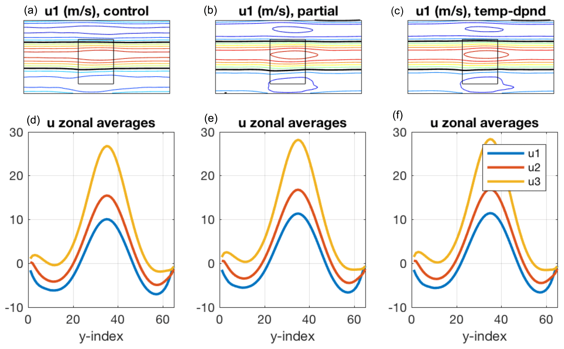
Figure 1 Atmospheric mean state in control (a, d), partially coupled (b, e), and fully coupled (c, f) simulations involving temperature-dependent wind in the atmospheric mixed layer. (a–c) Lower-layer zonal wind, CI = 2 m s⁻¹, the zero contour is black; rectangle in the middle (here and in other figures) marks the location of the ocean. (d–f) Zonally averaged zonal wind (m s⁻¹) in all layers (see legend).

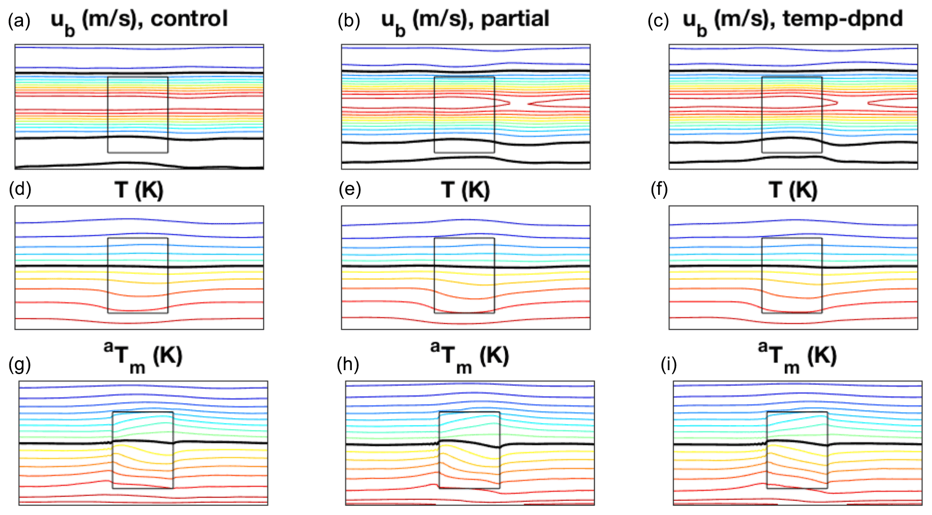
Figure 2 Atmospheric mean state (continued). (a–c) Barotropic zonal wind, CI = 2 m s⁻¹; (d–f) interior temperature perturbation according to Eq. (12), CI = 2 K; (g–i) AML temperature, CI = 2 K.

Figure 3 Atmospheric snapshots from the three simulations. (a–c) Lower-layer streamfunction; (d–f) AML temperature perturbation, CI = 2 K. Black curves show the zero contour.

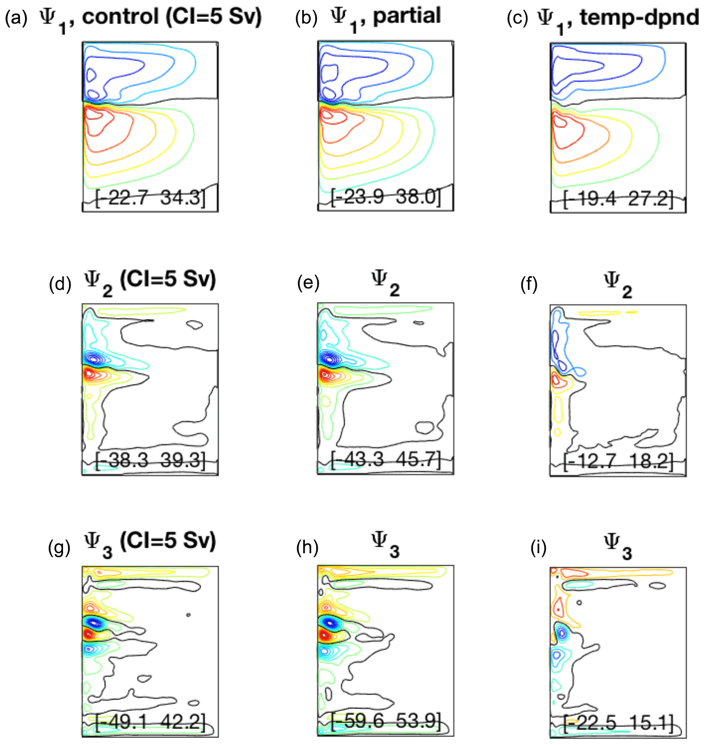
Figure 4 Oceanic time-mean streamfunction (Sv) in control (a, d, g), partially coupled (b, e, h), and fully coupled (c, f, i) simulations involving temperature-dependent wind in the atmospheric mixed layer. Top, middle, and bottom layer results are shown in the corresponding rows of the figure. CI is shown in panel captions. Black curves show the zero contour. The panels also display the range of streamfunction in Sv.

5 Model simulations

This section documents key characteristics of the new model versions described in Sects. 1–4. We set the amplitude of the variable incoming radiation $\left|F_{\mathrm{s}}^{\prime }\right|$ to 150 W m⁻² (as compared to 80 W m⁻² in Hogg et al., 2014) and ran three 130-year simulations of the new dry version of the model, as well as three analogous simulations of the new moist model, MQ-GCM (six simulations total), using model setups with and without temperature dependence in the atmospheric-mixed-layer wind. We ran the simulations for each model version to provide a preliminary assessment of the differences between different versions of the model. For both dry and moist versions of the model, the control run, without this dependence, was started from the final state of the preliminary 100-year spin-up simulation (from rest); the partially coupled simulation was initialized by the final state of the control run; and the fully coupled temperature-dependent simulation continued from the final state of the partially coupled run. We disregarded the first 30 years to allow for model spin-up and adjustment (chosen based on the ocean energy diagnostic) and analyzed the last 100 years of each simulation. Below we describe the results from the moist-model runs only; in the present parameter regime, the qualitative and quantitative behavior of the companion dry model turned out to be very similar, and hence the dry-model results are not shown here (see Sect. 6 for further discussion).

The atmospheric mean state does not appear to depend substantially on whether the temperature feedback on AML wind is included in the model or not. In each case the atmosphere is characterized by a straight climatological jet with a reasonable vertical shear (Fig. 1) and some zonal modulation; in particular, surface winds tend to be a bit stronger over ocean (due to reduced surface drag), but barotropic wind exhibits an opposite modulation (weaker wind over ocean), consistent with reduced temperature gradient over ocean (Fig. 2). On top of this mean state, the atmosphere is characterized by a vigorous synoptic turbulence (Fig. 3).

The time-mean ocean currents (Fig. 4) represent large-scale subtropical and subpolar gyres and strong inertial recirculations, which help maintain an intense eastward jet in the control and partially coupled simulations. The inertial recirculations largely collapse in the fully coupled simulation (see, for example, the discussion in Sect. 3 and Hogg et al., 2009), with barotropic transports there (∼40 Sv) only about one-third of those in the control and the partially coupled runs. Accordingly, the eastward jet becomes much weaker and so is the climatological SST front (Fig. 5); this has probably much to do with anomalous Ekman pumping structures over the inertial gyres seen in the fully coupled simulation (Fig. 5, bottom right). The ocean resolution (of 10 km) requires a relatively high viscosity (and low Reynolds number), and the ocean state can probably be characterized as eddy permitting rather than eddy resolving here (Fig. 6). The current simulations are only meant to illustrate a qualitative performance of the model. Simulations at higher resolutions (5 km) and Reynolds numbers may be advisable in all cases (cf. Martin et al., 2020).

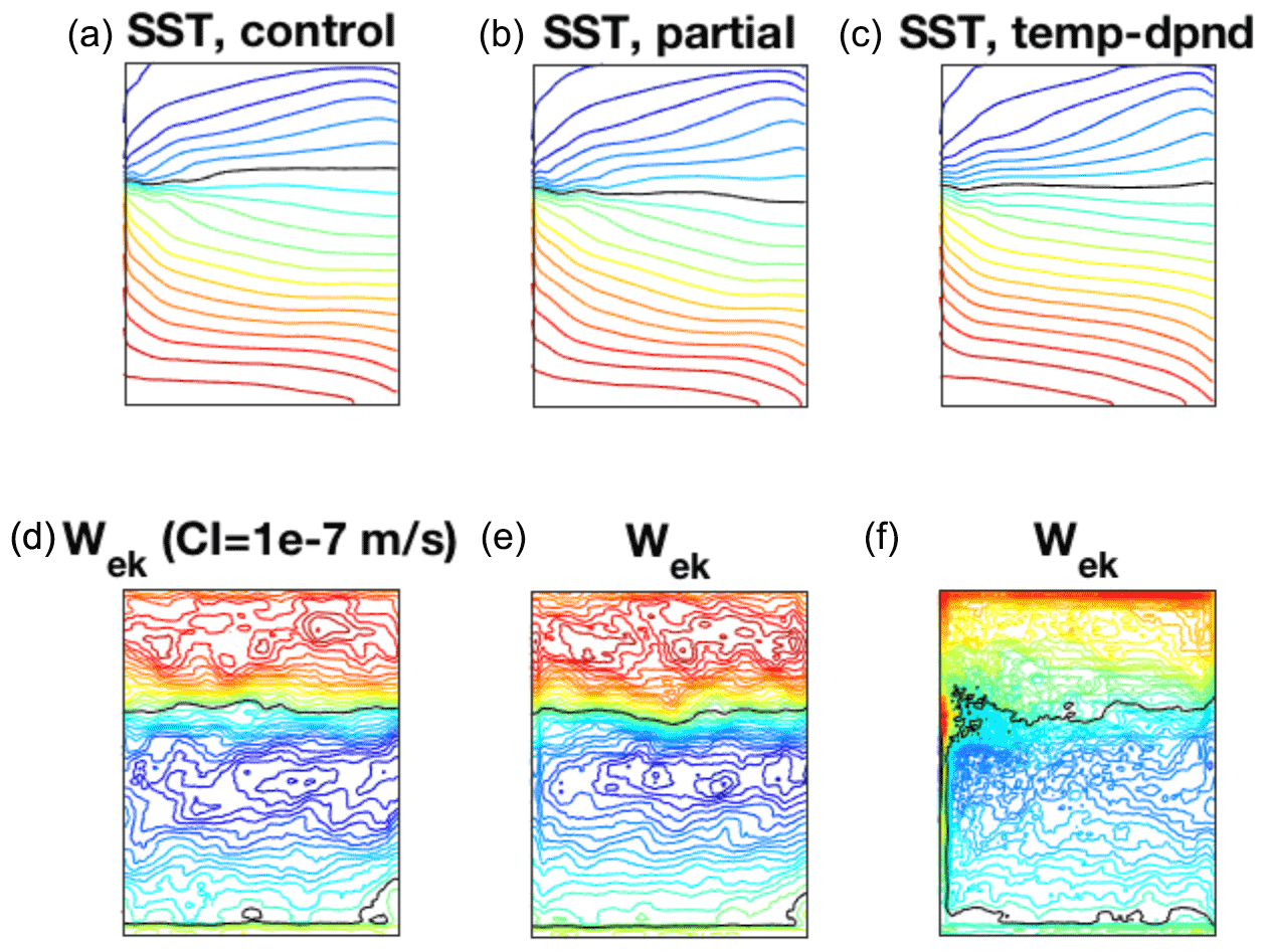
Figure 5 Time-mean SST (a–c, CI = 1 K) and ocean Ekman pumping (d–f, CI = 10⁻⁷ m s⁻¹) in control (a, d), partially coupled (b, e), and fully coupled (c, f) simulations involving temperature-dependent wind in the atmospheric mixed layer. Black line on SST plots shows −2 ^∘C anomaly with respect to the mean-state SST, approximately indicating the location of SST front; black line shows the zero contour on Ekman pumping plots.

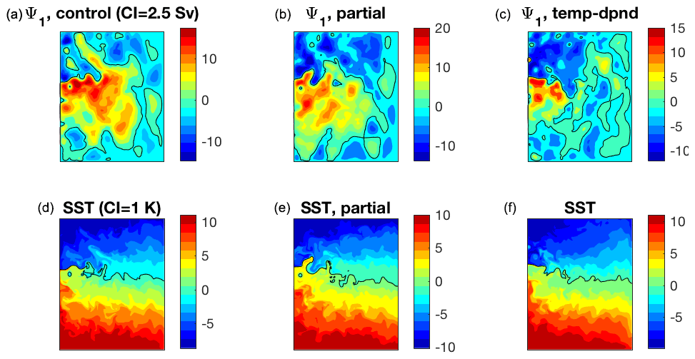
Figure 6 Oceanic snapshots from the three simulations. (a–c) Upper layer streamfunction (Sv); (d–f) OML temperature perturbation (K).

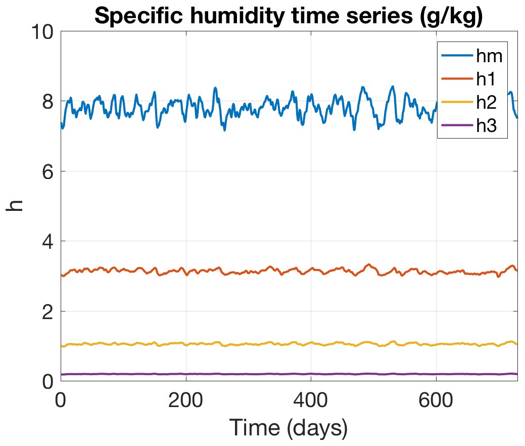
Figure 7 Time series of the basin-mean specific humidity (g kg⁻¹) in the four atmospheric layers (see the legend).

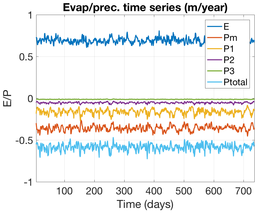
Figure 8 Time series of the basin-mean evaporation (positive) and layer precipitation (negative) (m yr⁻¹); see the legend.

Figure 9 Climatological distribution of specific humidity (g kg⁻¹).

We now show the moist characteristics of the model in the control simulation with dry entrainment formulation (23)–(24) of moisture entrainment fluxes in Eq. (34). Figure 7 displays a segment of the basin-mean specific humidity time series for all three atmospheric layers, featuring a reasonable vertical distribution of this quantity. The basin-mean moisture budget time series are shown in Fig. 8. The net evaporation and precipitation in the model are both around 0.6 m yr⁻¹, which is lower than the observed global-mean values of about 1 m yr⁻¹ due to the lack of tropical dynamics in the QG formulation. The basin-mean E–P is slightly unbalanced, indicating a small moisture flux of about 0.1 m yr⁻¹ through the open boundaries of the model (see Sects. 3.4 and 4). The specific humidity climatological distributions (Fig. 9) are slightly zonally nonuniform due to land–sea contrast and have patterns generally consistent with the atmospheric temperature distributions in Fig. 2.

Figure 10 Climatological distribution of evaporation (left) and precipitation in the mixed layer (right) (m yr⁻¹).

Figure 11 Climatological distribution of precipitation (m yr⁻¹); all layers.

Figure 12 Snapshot of precipitation (mm d⁻¹); all layers.

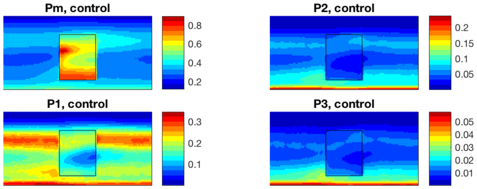
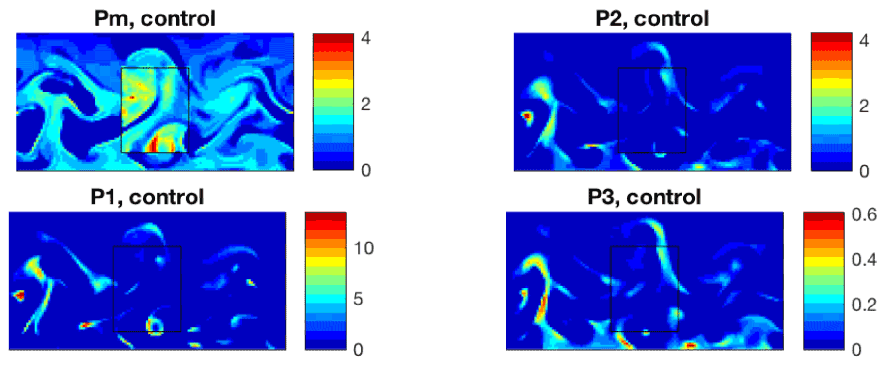
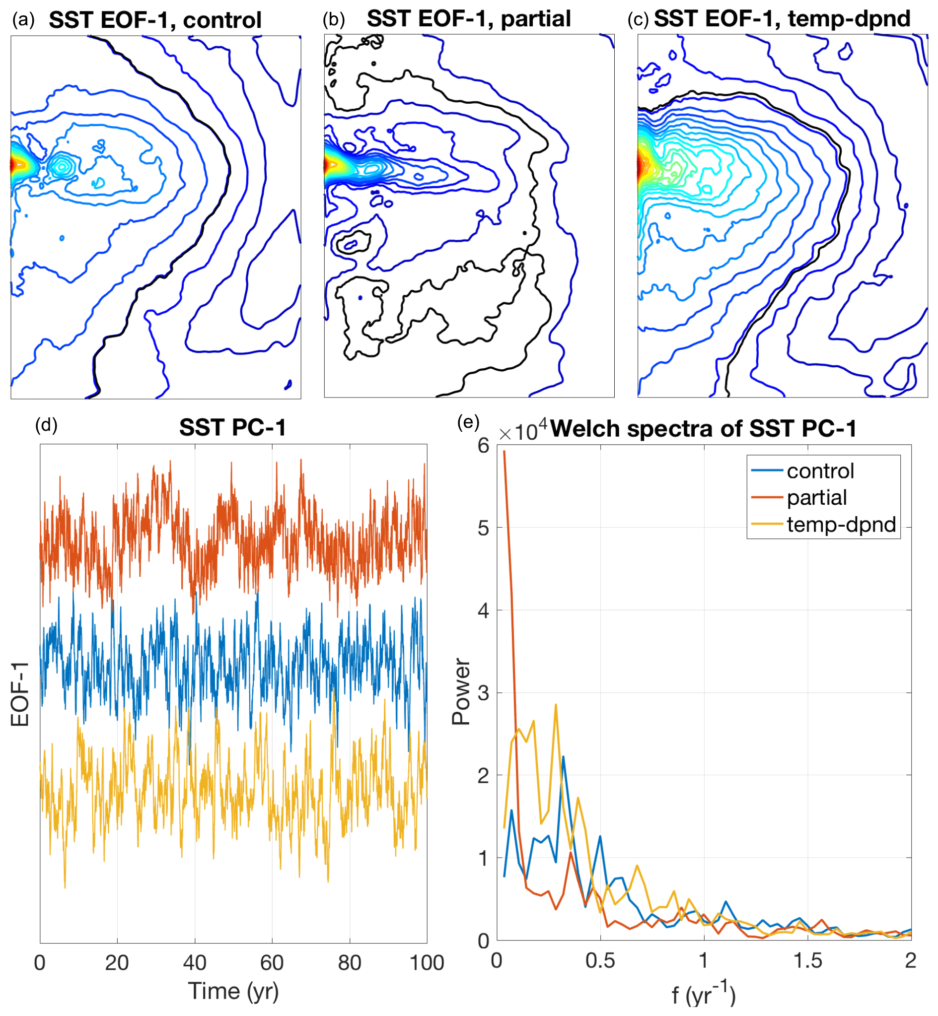
Figure 13 The leading EOF of SST. (a–c) EOF pattern in control (a), partially coupled (b), and full temperature-dependent momentum coupling (c) simulations; the zero contour is black. (d, e) PC-1 (d) and Welch-periodogram spectra (e) (the type of the simulation corresponding to each curve shown is given in the legend).

The evaporation (Fig. 10, left) is prescribed and zonally uniform over land (see Sect. 4) but is active over ocean, exhibiting reduced values to the north and enhancement along the southern and western boundary of the ocean and the double-gyre confluence zone. Atmospheric boundary layer precipitation is also enhanced over these areas (Fig. 10, right) and exhibits relative minima over the rest of the ocean. Globally, precipitation reaches local maximum at the southern boundary of the model and global minimum at the northern boundary and has a dipolar zonal structure around the axis of the channel, with precipitation minimum/maximum at the anticyclonic(equatorward)/cyclonic(poleward) flanks of the midlatitude jet, respectively. These features also translate, to some extent, to the precipitation distribution in the atmospheric interior (Fig. 11), although land–sea contrast in precipitation in the interior is opposite in sign to the one within the atmospheric boundary layer. The climatological distribution of precipitation is the result of averaging over intermittent, in space and time, precipitation episodes, as illustrated by a snapshot example in Fig. 12.

Finally, we present here initial evidence for an important effect of the temperature-dependent wind-stress formulation on the low-frequency dynamics of MQ-GCM. This effect can be noticed in the behavior of the leading EOF of SST (Fig. 13), which is dominated, in all simulations, by a monopolar (in y) SST pattern in the region of the ocean's eastward jet and its extension. The intensity, meridional localization, and west-to-east scale of this pattern are the largest in the partially coupled run, which has the strongest oceanic turbulence capable of affecting mesoscale winds above the oceanic eastward jet (Fig. 13, top middle panel). This variability tends to be suppressed in both the control run (with no direct SST effect on the AML winds: Fig. 13, top left panel) and the fully coupled run with active mesoscale coupling (but in which the ocean eddies are partly suppressed: Fig. 13, top right panel), indicating the importance of both the ocean eddies and air–sea mesoscale coupling for this mode. Furthermore, this mode's time dependence is characterized by a pronounced interdecadal variability in the partially coupled simulation, whereas the dominant timescales in the control and fully coupled simulations are shorter (interannual-to-decadal) and the associated variances are smaller (Fig. 13, bottom row), with the energy-density ratio of the partially coupled to control run of about 6 at low frequencies. It is not immediately clear, however, whether this mode imprints itself onto the atmosphere even in the partially coupled simulation. There are indications that this run's leading jet-shifting EOF of the atmospheric streamfunction (analogous to that of the control run shown in the top panel of Fig. 14) has an enhanced energy at the low-frequency end of the spectrum compared to the control and fully coupled simulations (Fig. 14, bottom), but this enhancement is not statistically significant and may be due to sampling. Longer and – most importantly – more highly resolved simulations, in both the ocean and the atmosphere (cf. Martin et al., 2020), are required to gauge the potential of the active mesoscale air–sea coupling to fuel decadal climate modes.

Figure 14 The leading EOF of the mid-layer atmospheric streamfunction. (a) EOF pattern in the control simulation. (b) Smoothed Welch-periodogram spectra of PC-1 in each simulation (the type of the simulation corresponding to each curve shown is given in the legend).

Table 2 Differences between updated and original Q-GCM formulation.

Table 3 Changes in the source code.

6 Discussion and conclusions

Note that the dynamical core of the present MQ-GCM model is identical to that of the original Q-GCM model, which has already been used in a suite of studies addressing midlatitude climate variability, while the newly added physics elements have been tested and verified in ocean-only or atmosphere-only settings (e.g., temperature-dependent wind stress: Feliks et al., 2004, 2007; Hogg et al., 2009) or are largely analogous, in their numerical formulation, to the previous Q-GCM elements (e.g., the moisture advection and time stepping scheme is analogous to that of the mixed-layer temperature), or are borrowed from similar ocean-only or coupled models (e.g., evaporation and latent-heat exchange parameterizations borrow from Kravtsov et al., 2006, and Deremble et al., 2012, 2013). The novelty of the present model is in that all these elements are brought together in a fully coupled setting, which makes it a unique numerically efficient tool for exploring possible dynamics of the midlatitude coupled climate variability. While of intermediate complexity, the model is still fairly involved, and no reference analytical solutions to directly verify the accuracy of its numerical implementation are available. Furthermore, it is well known from decades of numerical experimentation with analogous ocean-only models (see, e.g., Sect. 1 and references therein) that the regimes of simulated geostrophic turbulence strongly depend on the model's effective Reynolds number, with larger values of this number achievable at a higher horizontal resolution. An analogous statement pertains to frontal air–sea interactions, which may be sensitive to the horizontal resolution in the atmospheric component of the model (see Feliks et al., 2004, 2007). Future studies of the model sensitivity to the horizontal resolution, in the parameter regimes with high Reynolds numbers and mesoscale-resolving atmosphere are perhaps the ones to bring about the most interesting dynamical insights.

In the present model development effort, we only utilized eddy-permitting ocean resolution and a coarse-grid atmospheric model, which may be behind the similarity between the dry-model and moist-model behavior noted in Sect. 5. Overall, the MQ-GCM model exhibits rich moisture dynamics reminiscent of many of the observed properties of the Earth's climate system. It remains to be seen whether these and other processes (such as mesoscale air–sea coupling) affect in fundamental ways the dynamics of the midlatitude ocean–atmosphere system's coupled decadal variability. Preliminary results above indicate that the model's low-frequency variability is indeed sensitive to the details of air–sea interaction; furthermore, both dry and moist versions of the atmospheric model – in parameter ranges corresponding to strong thermal driving and intermediate surface drag (e.g., C_D=0.0005) – now exhibit bimodality of the type documented in Kravtsov et al. (2005, 2006, 2007, 2008), which is likely to be important for any decadal climate modes supported by the model (not shown here).

7 Summary of model updates and code modifications

Changes to the model formulation are summarized below in Table 2. Table 3 outlines the corresponding changes in the Q-GCM source code.

Appendix A: QGPV equation in a layered atmospheric model

Consider an ideal-gas dry atmosphere comprised of layers with constant potential temperatures θ_k. Using the definition of potential temperature, using the ideal gas law, and assuming hydrostatic balance (and dropping, in this section, the left superscript “a” that denotes atmospheric variables in the main text),

$$\begin{array}{}\text{(A1)}& \mathit{\theta }=T{\left({\displaystyle \frac{P_{\mathrm{0}}}{P}}\right)}^{\frac{R}{C_p}};P=\mathit{\rho }RT;{\displaystyle \frac{\partial P}{\partial z}}=-\mathit{\rho }g,\end{array}$$

one can express the pressures within each layer P_k as

$$\begin{array}{}\text{(A2)}& P_k^{\frac{R}{C_p}}=-P_{\mathrm{0}}^{\frac{R}{C_p}}{\displaystyle \frac{z}{H_{\mathit{\theta }k}}}+C_k\left(x,y\right);H_{\mathit{\theta }k}\equiv {\displaystyle \frac{C_p{\mathit{\theta }}_k}{g}}.\end{array}$$

The perturbation fields C_k can be found by requiring the pressure to be continuous across each atmospheric interface, namely

$$\begin{array}{}\text{(A3)}& \begin{array}{rl}{P}_{\mathrm{1}}{\mathrm{|}}_{H_{\mathrm{m}}}& =P_{\mathrm{m}}\left(x,y,t\right);P_{\mathrm{1}}{\mathrm{|}}_{H_{\mathrm{m}}+H_{\mathrm{1}}+{\mathit{\eta }}_{\mathrm{1}}}\\ & =P_{\mathrm{2}}{\mathrm{|}}_{H_{\mathrm{m}}+H_{\mathrm{1}}+{\mathit{\eta }}_{\mathrm{1}}};P_{\mathrm{2}}{\mathrm{|}}_{H_{\mathrm{m}}+H_{\mathrm{1}}+H_{\mathrm{2}}+{\mathit{\eta }}_{\mathrm{2}}}\\ & =P_{\mathrm{3}}{\mathrm{|}}_{H_{\mathrm{m}}+H_{\mathrm{1}}+H_{\mathrm{2}}+{\mathit{\eta }}_{\mathrm{2}}},\end{array}\end{array}$$

where P_m is the pressure at the top of the atmospheric mixed layer. For example, from Eqs. (A1)–(A3) we have, for the first atmospheric layer,

$$\begin{array}{}\text{(A4a)}& T_{\mathrm{1}}={\mathit{\theta }}_{\mathrm{1}}{F}_{\mathrm{1}};P_{\mathrm{1}}=P_{\mathrm{0}}{F}_{\mathrm{1}}^{\frac{C_p}{R}};{\mathit{\rho }}_{\mathrm{1}}={\displaystyle \frac{P_{\mathrm{0}}}{R{\mathit{\theta }}_{\mathrm{1}}}}{F}_{\mathrm{1}}^{\frac{C_p}{R}-\mathrm{1}},\end{array}$$

where

$$\begin{array}{}\text{(A4b)}& F_{\mathrm{1}}\left(x,y,z,t\right)={\left({\displaystyle \frac{P_{\mathrm{m}}}{P_{\mathrm{0}}}}\right)}^{\frac{R}{C_p}}-{\displaystyle \frac{(z-H_{\mathrm{m}})}{H_{\mathit{\theta }\mathrm{1}}}}.\end{array}$$

From Eq. (A4), the horizontal pressure gradient force in this layer is

$$\begin{array}{}\text{(A5a)}& -{\displaystyle \frac{\mathrm{1}}{{\mathit{\rho }}_{\mathrm{1}}}}\mathrm{\nabla }{P}_{\mathrm{1}}=-\mathrm{\nabla }{C}_p{\mathit{\theta }}_{\mathrm{1}}{\left({\displaystyle \frac{P_{\mathrm{m}}}{P_{\mathrm{0}}}}\right)}^{\frac{R}{C_p}}=-\mathrm{\nabla }{\mathit{\psi }}_{\mathrm{1}}{f}_{\mathrm{0}}.\end{array}$$

Here, the lower layer streamfunction ψ₁ is given by

$$\begin{array}{}\text{(A5b)}& {\mathit{\psi }}_{\mathrm{1}}={\displaystyle \frac{C_p{\mathit{\theta }}_{\mathrm{1}}}{f_{\mathrm{0}}}}{\left({\displaystyle \frac{P_{\mathrm{m}}}{P_{\mathrm{0}}}}\right)}^{\frac{R}{C_p}}\approx {\displaystyle \frac{C_p\stackrel{\mathrm{‾}}{\mathit{\theta }}}{f_{\mathrm{0}}}}{\left({\displaystyle \frac{P_{\mathrm{m}}}{P_{\mathrm{0}}}}\right)}^{\frac{R}{C_p}},\end{array}$$

where $\stackrel{\mathrm{‾}}{\mathit{\theta }}\sim \mathrm{300}$ K is the representative atmospheric potential temperature taken here to be equal, approximately, to the vertical average of individual-layer potential temperatures. In an analogous way, we find, for streamfunctions in layers 2 and 3,

$$\begin{array}{}\text{(A5c)}& {\displaystyle }\begin{array}{rl}{\mathit{\psi }}_{\mathrm{2}}& ={\displaystyle \frac{C_p{\mathit{\theta }}_{\mathrm{2}}}{f_{\mathrm{0}}}}\left({\left({\displaystyle \frac{P_{\mathrm{m}}}{P_{\mathrm{0}}}}\right)}^{\frac{R}{C_p}}-\left({\displaystyle \frac{\mathrm{1}}{H_{\mathit{\theta }\mathrm{1}}}}-{\displaystyle \frac{\mathrm{1}}{H_{\mathit{\theta }\mathrm{2}}}}\right){\mathit{\eta }}_{\mathrm{1}}\right)\\ & \approx {\mathit{\psi }}_{\mathrm{1}}-{\displaystyle \frac{g_{\mathrm{1}}^{\prime }{\mathit{\eta }}_{\mathrm{1}}}{f_{\mathrm{0}}}},\end{array}\text{(A5d)}& {\displaystyle }\begin{array}{rl}{\mathit{\psi }}_{\mathrm{3}}& ={\displaystyle \frac{C_p{\mathit{\theta }}_{\mathrm{3}}}{f_{\mathrm{0}}}}\left({\left({\displaystyle \frac{P_{\mathrm{m}}}{P_{\mathrm{0}}}}\right)}^{\frac{R}{C_p}}-\left({\displaystyle \frac{\mathrm{1}}{H_{\mathit{\theta }\mathrm{1}}}}-{\displaystyle \frac{\mathrm{1}}{H_{\mathit{\theta }\mathrm{2}}}}\right){\mathit{\eta }}_{\mathrm{1}}\right.\\ & \left.-\left({\displaystyle \frac{\mathrm{1}}{H_{\mathit{\theta }\mathrm{2}}}}-{\displaystyle \frac{\mathrm{1}}{H_{\mathit{\theta }\mathrm{3}}}}\right){\mathit{\eta }}_{\mathrm{2}}\right)\approx {\mathit{\psi }}_{\mathrm{2}}-{\displaystyle \frac{g_{\mathrm{2}}^{\prime }{\mathit{\eta }}_{\mathrm{2}}}{f_{\mathrm{0}}}},\end{array}\end{array}$$

where we assumed that the differences between the potential temperatures of individual layers are small compared to $\stackrel{\mathrm{‾}}{\mathit{\theta }}$ and estimated reduced gravities as

$$\begin{array}{}\text{(A6)}& g_k^{\prime }=g{\displaystyle \frac{{\mathit{\theta }}_{k+\mathrm{1}}-{\mathit{\theta }}_k}{\stackrel{\mathrm{‾}}{\mathit{\theta }}}}.\end{array}$$

From Eq. (A5) it follows that

$$\begin{array}{}\text{(A7)}& {\mathit{\eta }}_k=f_{\mathrm{0}}{\displaystyle \frac{{\mathit{\psi }}_k-{\mathit{\psi }}_{k+\mathrm{1}}}{g_k^{\prime }}}\end{array}$$

and that the “dynamic pressures”  ^ap_k in Hogg et al. (2014) are equal to f₀ψ_k.

Furthermore, under synoptic scaling, the continuity equation in each layer is approximately

$$\begin{array}{}\text{(A8)}& {\displaystyle \frac{\partial u}{\partial x}}+{\displaystyle \frac{\partial v}{\partial y}}+{\displaystyle \frac{\partial w}{\partial z}}-{\displaystyle \frac{w}{H_{\mathit{\theta }k}}}=\mathrm{0},\end{array}$$

but the last term on the right-hand side of Eq. (A8) – approximating $\frac{w}{\mathit{\rho }}\frac{\partial \mathit{\rho }}{\partial z}$ – is smaller than other terms and can be neglected under QG scaling, since H_θk≃30 km and $H_k/H_{\mathit{\theta }k}\sim \mathrm{0.1}$ is on the order of the Rossby number.

Thus, the above scaling arguments and calculations demonstrate the validity of Boussinesq approximation for quasi-geostrophic compressible atmosphere and justify the uniform treatment of oceanic and atmospheric dynamics in Hogg et al. (2014).