MUNICH v2.0: a street-network model coupled with SSH-aerosol (v1.2) for multi-pollutant modelling

A new version of a street-network model, the Model of Urban Network of Intersecting Canyons and Highways version 2.0 (MUNICH v2.0), is presented. The comprehensive aerosol model SSH-aerosol is implemented in MUNICH v2.0 to simulate the street concentrations of multiple pollutants, including secondary aerosols. The implementation uses the application programming interface (API) technology so that the SSH-aerosol version may be easily updated. New parameterisations are also introduced in MUNICH v2.0, including a non-stationary approach to model reactive pollutants, particle deposition and resuspension, and a parameterisation of the wind at roof level. A test case over a Paris suburb is presented for model evaluation and to illustrate the impact of the new functionalities. The implementation of SSH-aerosol leads to an increase of 11 % in PM₁₀ concentration because of secondary aerosol formation. Using the non-stationary approach rather than the stationary one leads to a decrease in NO₂ concentration of 16 %. The impact of particle deposition on built surfaces and road resuspension on pollutant concentrations in the street canyons is low.

1 Introduction

More than half of the global population now lives in urban areas (Ritchie and Roser, 2018), and is often exposed to high concentrations of nitrogen dioxide (NO₂) and fine particulate matter (PM) with diameters lower than and equal to 2.5 µm (PM_2.5, Krzyzanowski et al., 2014). In numerous cities, there are densely built districts with street-canyon configurations. Street-level air quality has been reported to be worse than that in the surrounding area because of the presence of air pollutant sources. In particular, high concentrations of NO₂ (Cyrys et al., 2012), black carbon (Putaud et al., 2010; Lugon et al., 2021b), and organics have been reported (Putaud et al., 2010; Airparif, 2011).

Air quality models provide a useful tool to understand the phenomenon of pollution in street canyons (Lugon et al., 2021b) and to estimate the impact of emission scenarios to reduce pollution. Different types of models may be used to represent the pollution in street canyons. Computational fluid dynamics (CFD) models, e.g. Code_Saturne (Milliez and Carissimo, 2007; Thouron et al., 2019), OpenFOAM (Jeanjean et al., 2015; Wu et al., 2021), STAR-CCM+ (Santiago et al., 2017), and the PALM model (Wolf et al., 2020; Zhang et al., 2021), finely describe the urban geometry, the air flow, and the pollutant concentrations. However, the computational cost is too high for operational purposes if they are applied to predict the pollutant concentrations in a city district with a large street network (at least hundreds of street segments) (Vardoulakis et al., 2003). Parametric models are another type. They are suitable for operational purposes because of their low computational cost. Some parametric models, e.g. Polyphemus (Briant et al., 2013) and CALINE4 (Benson, 1992), are based on the use of a Gaussian dispersion methodology to represent emitted traffic-related pollutants, such as a Gaussian plume or puff. Because they can not represent a street-canyon configuration, they are modified to include a specific module to represent this particular geometry, e.g. OSPM (Berkowicz, 2000), SBLINE (Namdeo and Colls, 1996), and ADMS-Urban (McHugh et al., 1997). Other parametric models use parameterisations based on CFD modelling or wind-tunnel experiments to describe the flow in each street and the exchange from street to street and between streets and the overlying atmosphere. The transport of pollutants from one street to another is taken into account through intersections, e.g. SIRANE (Soulhac et al., 2011) and the Model of Urban Network of Intersecting Canyons and Highways (MUNICH) (Kim et al., 2018). The flow above the street network is represented by a Gaussian dispersion methodology (SIRANE) or by one- or two-way nesting in a regional model (MUNICH).

The streets are discretised with an Eulerian approach and boxes representing the street-segment volumes. Breaking away from the Gaussian methodology, this approach allows one to model the reactivity of pollutants as they are transported from the regional scale (background concentrations) to the street. Lugon et al. (2020) showed that it is crucial to couple the transport of pollutants in the street and chemistry finely, using a non-stationary approach that avoids a steady-state assumption, in order to represent the concentrations of reactive pollutants such as NO₂. By coupling MUNICH to the aerosol model SSH-aerosol (Sartelet et al., 2020), Lugon et al. (2021a) showed that the formation of secondary aerosols is important not only at the regional scale, but also at the street level. This paper presents version 2.0 of MUNICH. The different model improvements of Lugon et al. (2020, 2021a) have been implemented, as well as the modelling of deposition and resuspension from Lugon et al. (2021b). The coupling to the SSH-aerosol model has been improved and automated. New parameterisations of the flow in the street have also been added. A reference test case is presented for model evaluation and to illustrate the behaviour and capabilities of MUNICH.

A description of the model is given and the major updates made from v1.0 to v2.0 are summarised in Sect. 2. Section 3 presents the simulation domain and the setup of the reference test case, which is compared to observations of NO₂, nitric oxide (NO), PM_2.5, and particulate matter with diameters lower than 10 µm (PM₁₀). In Sects. 4, 5, and 6, different sensitivity simulations are presented to understand how these updates influence the street concentrations. They are classified depending on whether they concern transport (Sect. 4), chemistry (Sect. 5), or deposition/resuspension (Sect. 6). Finally, two other sensitivity simulations of important parameters for the modelling and applications of MUNICH are performed (the influence of the building aspect ratio and the effects of removing car traffic from specific streets).

2 Description of the model and major updates

Version 1.0 of MUNICH is described in Kim et al. (2018). Only the main concepts are reviewed here. In MUNICH, a street network is divided into street segments and intersections. A street segment is bounded by intersections with other street segments. A street segment is represented by one cuboid-type box, and concentrations are assumed to be homogeneous in the corresponding volume, which is estimated as the product of the segment length and width and the average building height. The fluxes of pollutants emitted in a street segment due to human activities and natural sources (e.g. trees) are diluted within this volume. Pollutant concentrations are only evaluated in each street segment and not at intersections, which are defined to represent the street-to-street advective transfer of pollutants and part of the exchanges with the overlying atmosphere (Soulhac et al., 2009). The exchanges between a street segment and the overlying atmosphere are also computed at the top of each street segment. If the formulation of Salizzoni et al. (2009) is used, they depend on the standard deviation of the vertical wind velocity at roof level, which depends on the atmospheric stability, and on the concentration gradients between the street and above. As detailed in MUNICH v1.0 (Kim et al., 2018), this formulation may be modified to take into account the influence of the street ratio ($H/W$), as suggested by Schulte et al. (2015) and detailed in Appendix B.

Pollutants are also advected from street to street after averaging the vertical wind profile in the street. This profile depends on the wind velocity at the roof level, which itself depends on the meteorological data above the streets (e.g. wind speed and direction) and the street segment characteristics (e.g. street segment direction, street width, building height). As detailed in MUNICH v1.0, two formulations may be used to represent the wind profile within the streets: the exponential formulation (Lemonsu et al., 2004) or the analytical formulation from SIRANE (Soulhac et al., 2008). These formulations depend on the wind velocity at the roof level u_H (see Appendix B), for which a new formulation is proposed here (see Sect. 2.2, based on the work of Macdonald et al., 1998).

The emission may occur in both the gas and particle phases. The chemical transformations of the pollutants are modelled by a chemical kinetic mechanism for the gas phase and/or by an aerosol model representing the aerosol dynamics (nucleation, condensation/evaporation, and coagulation) and mass transfer between the gas and particle phases.

The loss fluxes due to deposition are represented through parameterisations of dry deposition and wet scavenging. An approach to estimate resuspension is added in MUNICH v2.0, following Lugon et al. (2021b).

Many modelling options are included to represent the different physico-chemical processes taken into account in MUNICH. They are presented in Appendix B. A demonstration test case is set up in Sect. 2.1 to illustrate how the pollutants are transported within the street network from a single emission source. This test case is used to validate both versions of MUNICH. Then, the section describes the new features in comparison to MUNICH v1.0.

2.1 Advection through intersections

At intersections, the pollutant mass flux from one street to others can be computed by estimating the balance of the air-volume fluxes among the streets that are connected to the intersection.

A simplified street network with 12 street segments was designed to perform a theoretical test case and illustrate how mass fluxes are modelled. For simplicity, the wind speed at rooftops was fixed to an arbitrary value (5 or 10 m s⁻¹), and a pollutant was emitted in only one street segment (number 11 in Fig. 1). Figure 1 displays the mass concentrations calculated using MUNICH in the different street segments (red numbers). The concentrations are the highest in the street segment where the pollutant is emitted. The concentrations vary depending on the wind direction above the streets. For higher wind speeds at the roof level (10 m s⁻¹, see Fig. 1d–f), the pollutant concentrations are lower over all street segments. This is due to an increase in the advection and also an increase in the vertical transfer by turbulence at rooftops.

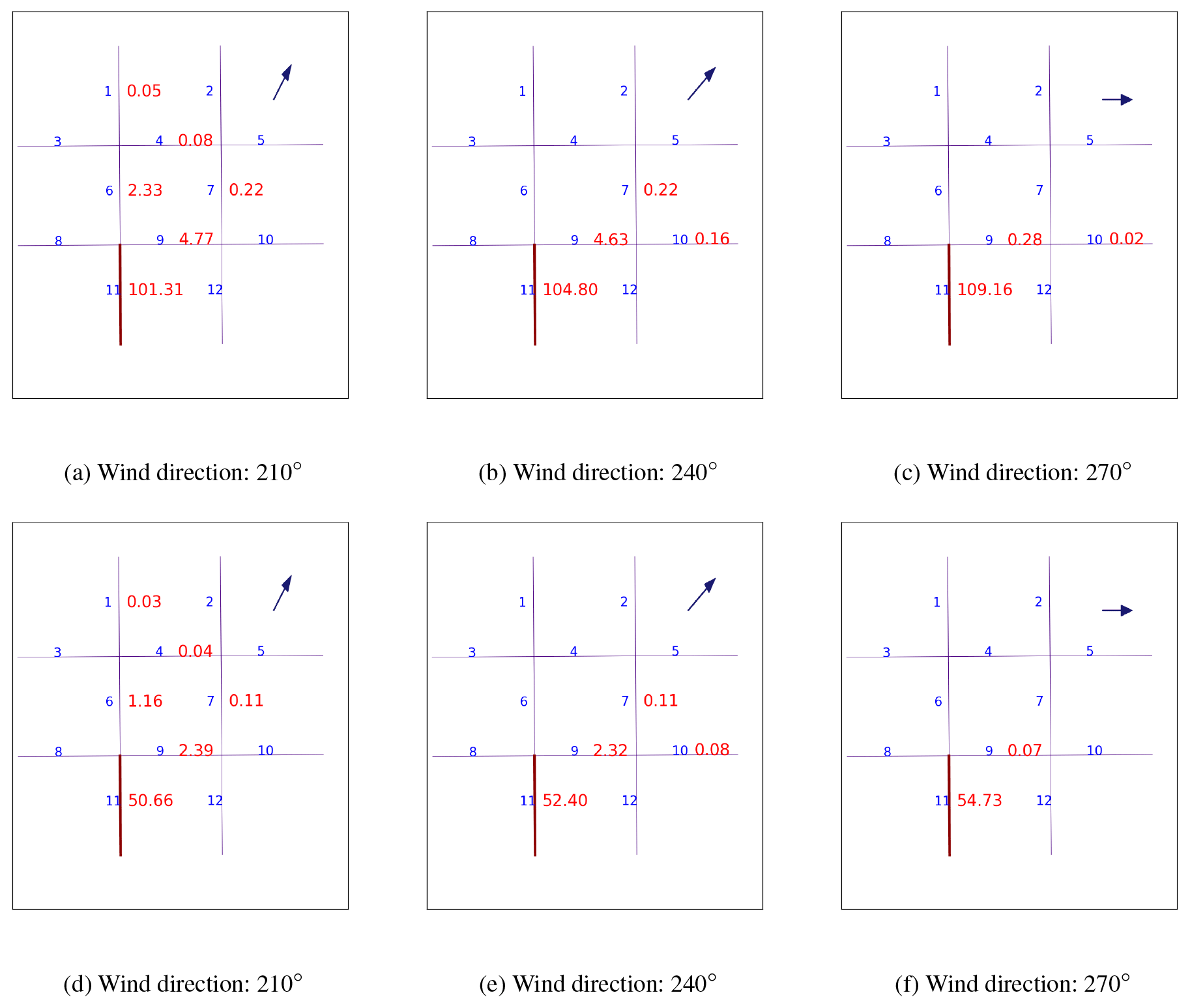
Figure 1 Variation of pollutant concentrations in a street network with wind direction, which are indicated as arrows in dark blue. The wind speed is 5 m s⁻¹ for (a), (b), and (c) and 10 m s⁻¹ for (d), (e) and (f). The wind direction is given from the north (top of the figure). The blue numbers are the street ID and the red numbers are the concentrations in µg m⁻³. A pollutant is only emitted in street segment 11.

2.2 Wind velocity at the roof level

The computation of the vertical wind profile within the street depends on the wind velocity determined at the roof level u_H (see Eqs. B12 and B13 from Appendix B). u_H was computed following Soulhac et al. (2008) in MUNICH v1.0, based on a 2D parameterisation of the wind field along the street axis. Now it may be computed depending on the street characteristics using a logarithmic wind profile above the buildings, as defined in Macdonald et al. (1998). This wind profile corresponds to an average profile over a relatively large urban-scale area, such as a relatively homogeneous district or city. It is based on the calculation of a displacement height (d_c) and a roughness length (z_0c) for the homogeneous urban canopy area (district) considered. Note that the roughness length of the district is typically on the order of 1 m (see Fig. 2), whereas those of street walls and road pavements are of the order of 1 mm.

$$\begin{array}{}\text{(1)}& {\displaystyle \frac{d_{\mathrm{c}}}{\stackrel{\mathrm{‾}}{H}}}& {\displaystyle }=\mathrm{1}+{\mathrm{\Delta }}^{-{\mathit{\lambda }}_{\mathrm{P}}}\left({\mathit{\lambda }}_{\mathrm{P}}-\mathrm{1}\right)\text{(2)}& {\displaystyle \frac{z_{\mathrm{0}\mathrm{c}}}{\stackrel{\mathrm{‾}}{H}}}& {\displaystyle }=\left(\mathrm{1}-{\displaystyle \frac{d_{\mathrm{c}}}{\stackrel{\mathrm{‾}}{H}}}\right)\exp \left(-{\left(\mathrm{0.5}\mathit{\delta }{\displaystyle \frac{C_{{\mathrm{D}}_{\mathrm{b}}}}{{\mathit{\kappa }}^{\mathrm{2}}}}\left(\mathrm{1}-{\displaystyle \frac{d_{\mathrm{c}}}{\stackrel{\mathrm{‾}}{H}}}\right){\mathit{\lambda }}_{\mathrm{F}}\right)}^{-\mathrm{0.5}}\right),\end{array}$$

where Δ and δ are empirical constants (δ=1.0 and Δ=4.43 for staggered arrays, which are are used in MUNICH v2.0; δ=0.55 and Δ=3.59 for square arrays; Macdonald et al., 1998); $C_{{\mathrm{D}}_{\mathrm{b}}}$ is the building drag coefficient, which is usually equal to 1.2 (Macdonald et al., 1998); and κ is the von Kármán constant (κ=0.41).

λ_P and λ_F are, respectively, the plan and frontal area densities of obstacles, calculated as

$$\begin{array}{}\text{(3)}& \begin{array}{rl}{\mathit{\lambda }}_{\mathrm{P}}& ={\displaystyle \frac{A_{\mathrm{P}}}{A_{\mathrm{T}}}}={\displaystyle \frac{\stackrel{\mathrm{‾}}{W_{\mathrm{building}}}\stackrel{\mathrm{‾}}{L}}{\left(\stackrel{\mathrm{‾}}{W_{\mathrm{building}}}+\stackrel{\mathrm{‾}}{W_{\mathrm{street}}}\right)\stackrel{\mathrm{‾}}{L}}}\\ & \text{and}{\mathit{\lambda }}_{\mathrm{F}}={\displaystyle \frac{A_{\mathrm{F}}}{A_{\mathrm{T}}}}={\displaystyle \frac{\stackrel{\mathrm{‾}}{H}\stackrel{\mathrm{‾}}{L}}{\left(\stackrel{\mathrm{‾}}{W_{\mathrm{building}}}+\stackrel{\mathrm{‾}}{W_{\mathrm{street}}}\right)\stackrel{\mathrm{‾}}{L}}}.\end{array}\end{array}$$

Here, A_F, A_P, and A_T are, respectively, the frontal, plan, and lot areas of obstacles (A_T corresponds to the total area divided by the number of obstacles). Those surface ratios are calculated from the average characteristics of the streets in the district considered: building height ($\stackrel{\mathrm{‾}}{H}$), street width ($\stackrel{\mathrm{‾}}{W_{\mathrm{street}}}$), building width ($\stackrel{\mathrm{‾}}{W_{\mathrm{building}}}$), and street length ($\stackrel{\mathrm{‾}}{L}$), which cancels in both equations.

Finally, u_H is calculated for each street of building height H as

$$\begin{array}{}\text{(4)}& u_H={\displaystyle \frac{u_{*}}{\mathit{\kappa }}}\ln \left({\displaystyle \frac{H-d_{\mathrm{c}}}{z_{\mathrm{0}\mathrm{c}}}}\right)=u_{\mathrm{ref}}\times {\displaystyle \frac{\ln \left(\frac{H-d_{\mathrm{c}}}{z_{\mathrm{0}\mathrm{c}}}\right)}{\ln \left(\frac{z_{\mathrm{ref}}-d_{\mathrm{c}}}{z_{\mathrm{0}\mathrm{c}}}\right)}}.\end{array}$$

Depending on the chosen input parameters, u_H can be calculated from the friction velocity u_* (in m s⁻¹) defined at urban canopy scale or from the wind speed at a reference altitude above the street (u(z_ref)=u_ref in m s⁻¹). For each street, only the axial component of u_H is considered when computing the average wind speed in the street direction. Therefore, the horizontal transport of pollutants in the street depends on the angle between the wind direction and the street orientation.

2.3 Concentrations of reactive species: non-stationary approach

In MUNICH v1.0, a first-order splitting scheme between “transport” (including removal processes) and chemistry is used to calculate the concentrations in a street segment with fixed splitting time steps (typically 100 s). This numerical approach holds for slowly reacting species, but it fails to represent the temporal evolution of fast-reacting species. The characteristic timescales of fast chemical processes may be similar to (or faster than) those of transport in and out the street. A new algorithm is presented in Lugon et al. (2020) to remove the steady-state assumption for transport (i.e. the stationary approach). At the first time iteration, the characteristic timescale of transport is estimated, and then transport and chemistry are solved sequentially on a time step corresponding to this characteristic time. Transport is solved using an explicit two-stage Runge–Kutta algorithm (explicit trapezoidal rule of order 2) or a semi-implicit Rosenbrock algorithm, and chemistry is solved with smaller time steps using a Rosenbrock algorithm or the solver used in SSH-aerosol (two-stage Runge–Kutta or two-step algorithms). The equations for gas-phase chemistry and aerosol dynamics (grouped here as “chemistry”) are solved using smaller time steps, because they correspond to a stiff set of equations with very fast processes such as radical chemistry. The time step is adapted depending on the evolution of the concentrations due to transport-related processes.

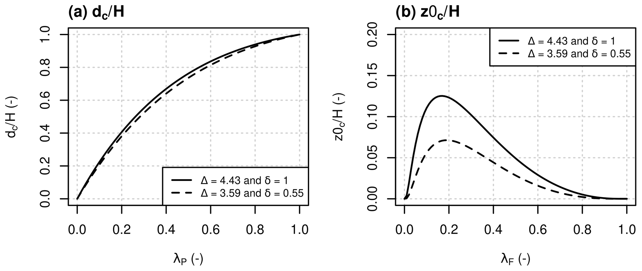
Figure 2 (a) $d_{\mathrm{c}}/\stackrel{\mathrm{‾}}{H}$ and (b) $z_{\mathrm{0}\mathrm{c}}/\stackrel{\mathrm{‾}}{H}$ as functions of the plan and frontal area densities (λ_P and λ_F) calculated by Eq. (3).

Using a beta version of MUNICH, Lugon et al. (2020) showed that this algorithm is numerically stable for reactive species, unlike the one using the stationary assumption. The effects of this new algorithm in MUNICH v2.0 are presented in Sect. 5.2.

2.4 Coupling to SSH-aerosol (v1.2)

The chemical composition of particles in streets differs from those above, mostly because of pollutants emitted within the streets, for example from traffic (Lugon et al., 2021a). Within the streets, emitted pollutants mix with those from above the streets and undergo chemistry. In MUNICH v1.0, only gas-phase chemistry is taken into account, and the CB05 chemical kinetic mechanism (Yarwood et al., 2005) is implemented to simulate the gas-phase concentrations (Kim et al., 2018).

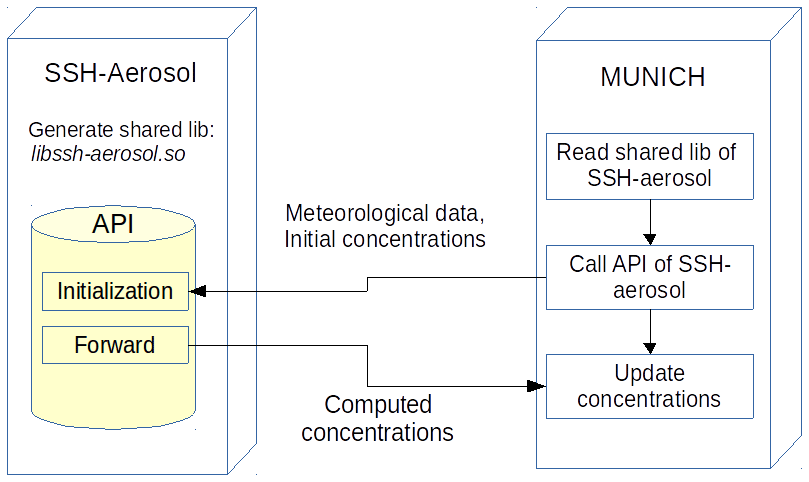
In MUNICH v2.0, the SSH-aerosol model (Sartelet et al., 2020) may be used to simulate both gas-phase chemistry and aerosol thermodynamics and dynamics (i.e. nucleation, condensation/evaporation, and coagulation). SSH-aerosol is designed to be easily implemented in other models. It contains an application programming interface (API) that is designed to allow for easy version updates. The API is used to implement SSH-aerosol v1.2 in MUNICH v2.0. A schematic diagram of coupling using the API is illustrated in Fig. 3. A previous version of SSH-aerosol was implemented in MUNICH without using the API (Lugon et al., 2021a); it satisfactorily reproduced measured PM₁₀ and PM_2.5 concentrations in the streets of Paris, taking into account the formation of secondary inorganic and organic aerosols. The influence of secondary aerosol formation is presented in Sect. 5.1.

Figure 3 Schematic diagram of the coupling of SSH-aerosol with MUNICH using the API.

2.5 Resuspension and deposition

Lugon et al. (2021b) introduced a new approach in MUNICH estimating particle resuspension in streets. This approach strictly ensures mass balance on the street surface. To do that, the accurate modelling of particle deposition and wash-off by water is mandatory. In MUNICH v2.0, the particle deposition is computed considering the available surface area, including pavement area and building walls, as proposed in Cherin et al. (2015). For the particle wash-off, the amount of water on the street surface is computed from the meteorological conditions. Solubility of species is also an important factor for the wash-off parameterisation.

Modelling of the particle resuspension in MUNICH v2.0 requires an estimation of a resuspension factor. The resuspension factor is computed considering the traffic flow characteristics such as vehicle flow and speed, as detailed in Lugon et al. (2021b). The sensitivity of concentrations to deposition and resuspension is presented in Sect. 6.

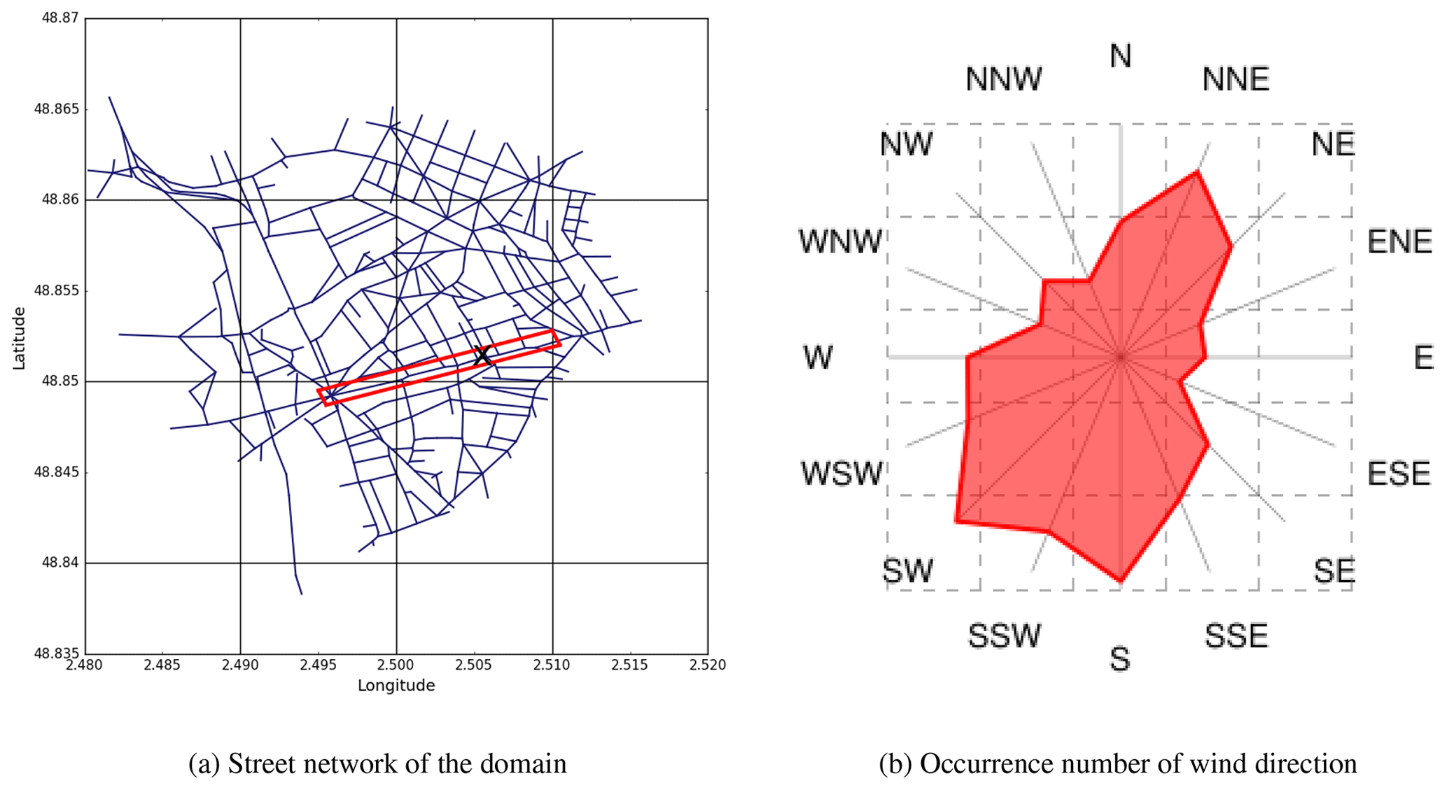
Figure 4 (a) Street network of the domain. The street named “Boulevard Alsace Lorraine”, where measurements were performed, is highlighted by the red box. The black cross mark corresponds to the location of the air monitoring station. (b) Occurrence number of each wind direction over the street network for the period from 22 March to 13 May 2014.

3 Reference test case

MUNICH v2.0 is applied to simulate the pollutant concentrations over a Paris suburb. The reference test case is set up over a district in the eastern part of Greater Paris between 22 March and 13 May 2014, which corresponds to a period when street measurements were performed, with samples taken at a height of about 3 m (TRAFIPOLLU project, see the location of the station in Fig. 4a). The street network of the domain consists of 577 street segments and is displayed in Fig. 4a. The input data used for this study are now detailed. They are summarised in Table 1. The simulated concentrations are then compared to street observations.

Leclercq et al. (2007)Kim et al. (2018)Lugon et al. (2020)Sartelet et al. (2018); André et al. (2020)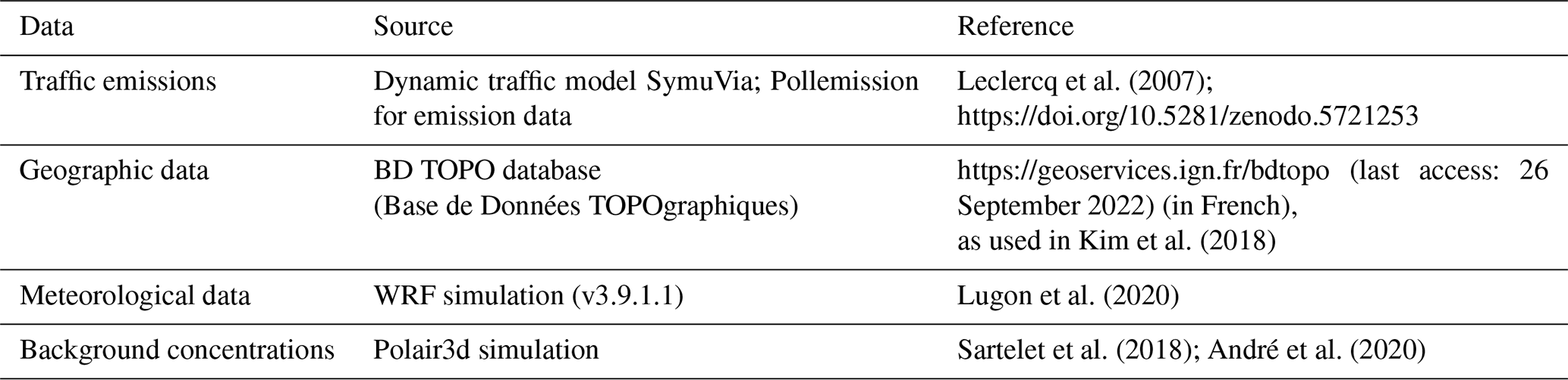

Table 1 Input data for MUNICH simulation.

3.1 Input data

3.1.1 Traffic emissions

Traffic-related emissions in streets are computed using Pollemission (Sarica, 2021), which relies on emission factors from the COPERT methodology (COmputer Program to calculate Emissions from Road Transport, version 2019, EMEP/EEA, 2019) and the vehicle fleet. Emission factors are provided by the COPERT methodology for a wide range of vehicle types, according to the fuel type and European emission standard of the vehicle. The COPERT methodology is used for both exhaust and non-exhaust emission factors, i.e. wear of the tyres and brakes and vehicle-induced abrasion of the road. Simulations using the dynamic traffic model SymuVia (Leclercq et al., 2007) provided, for each street segment of the network, the number of vehicles and the speed profile per hour and per category (passenger cars, light commercial vehicles, heavy-duty vehicles, …) for a weekday and a weekend day. The vehicle fleet is mainly composed of passenger cars and light commercial vehicles: 77 % and 14 %, respectively, on average. In each category, the breakdown by fuel and European standard is based on André et al. (2019). For each vehicle type, hourly profiles of vehicle flow and average speeds for a weekday and a weekend day are then used with COPERT emission factors to estimate the traffic emissions over the whole period (22 March to 13 May 2014).

Nitrogen oxide (NO_x) emission factors are speciated into NO and NO₂ using the fractions of NO₂ provided by the COPERT methodology for each vehicle type. Speciation of PM emission factors also follows the COPERT methodology by using the fractions of black carbon (BC) and organic matter (OM) supplied for each vehicle type. The OM fraction of the PM emissions is assumed to be emitted as low-volatility organic compounds (LVOC) in the particle phase. If a fraction of the PM remains after the BC and OM speciation, it is categorised as dust and unspeciated species. The PM size distribution at emission is assumed to be the same as in Lugon et al. (2021a, b), i.e. exhaust primary PM is assumed to be in the size bin 0.04–0.16 µm, while non-exhaust primary PM is coarser, i.e. in the size bin 0.4–10 µm.

Non-methane volatile organic compound (NMVOC) emission factors are computed as the difference between the volatile organic compounds (VOC) and the methane emission factors. In contrast to NO_x and PM, the COPERT methodology presents five NMVOC speciation profiles given the fuel and category of the vehicle. These profiles include approximately 60 different species up to about C9 (nine carbon atoms) and lumped species for heavier compounds. Intermediate-volatility organic compounds (IVOC) thus include the C10–C12 alkanes, cycloalkanes, C9 aromatics, and C10 aromatics. Similarly, semi-volatile organic compounds (SVOC) include the > C13 alkanes and > C13 aromatics. Both IVOC and SVOC are emitted in the gas phase in the simulation, and the partitioning between the gas and particle phases is treated by the model when computing concentrations.

3.1.2 Geographic data

The widths of vehicle lanes in the streets, street lengths, and average building heights are obtained from the BD TOPO database (Base de Données TOPOgraphiques, https://geoservices.ign.fr/bdtopo, last access: 26 September 2022). Information on the sidewalk width and the highway shoulder width (the A86 highway passes through the modelling domain) is not available in the BD TOPO database. A width of 3 m is used for sidewalks of the streets, and a width of 20 m (including two urban train lanes) is used for the shoulder of the A86 highway (Kim et al., 2018).

3.1.3 Regional-scale data

Meteorological data at 1 km × 1 km horizontal resolution are obtained from Lugon et al. (2020), who conducted a simulation using the Weather Research and Forecasting (WRF) model version 3.9.1.1 (Skamarock et al., 2008). In the WRF model setup, the single-layer urban canopy model (UCM) is used to represent the urban meteorological conditions (Kusaka et al., 2001). The meteorological data from the WRF simulation are updated every hour in the MUNICH simulations, and they are interpolated for the times between each hour. Figure 4b shows the occurrence number of each wind direction over the simulation domain for the period from 22 March to 13 May 2014. The occurrence of wind that comes from each compass direction (N, NNE, NE, etc.) is counted. South and southwest winds are the prevailing winds during the simulation period.

Background concentrations above the streets are obtained from the simulation results of the three-dimensional chemical-transport model Polair3D (Sartelet et al., 2007). The Polair3D simulation is presented in Sartelet et al. (2018); André et al. (2020). The same chemical scheme is used in the MUNICH simulation as in the Polair3D regional-scale simulation (CB05 with additional semi-volatile organic aerosols, as detailed in Kim et al., 2011, Chrit et al., 2017, and Sartelet et al., 2020).

Table 2 List of options used in the reference simulation.

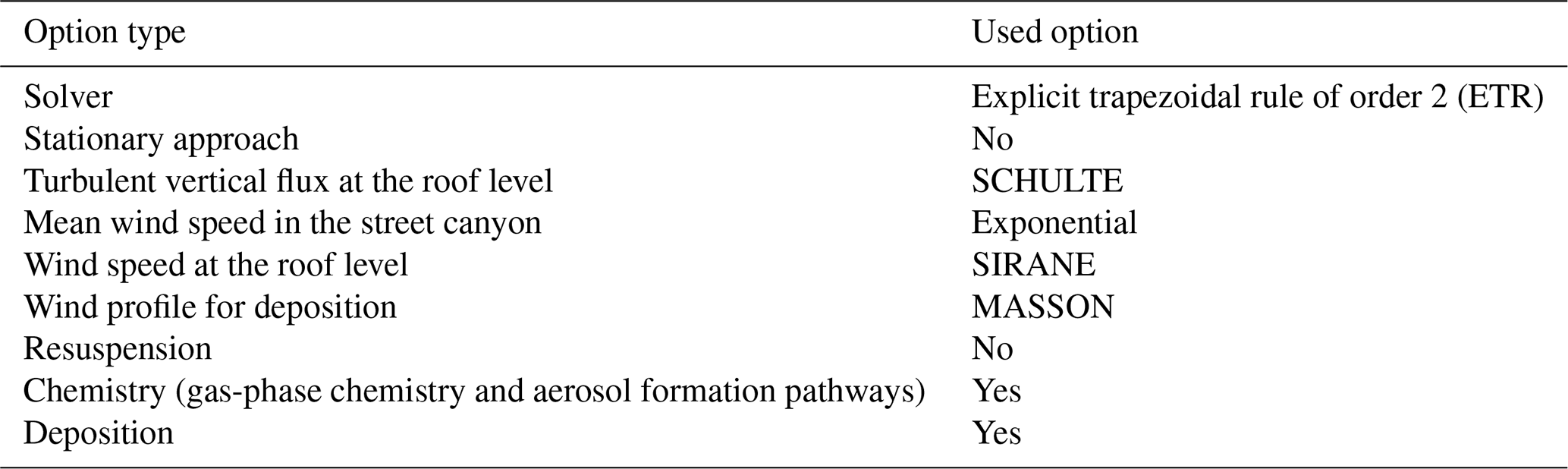
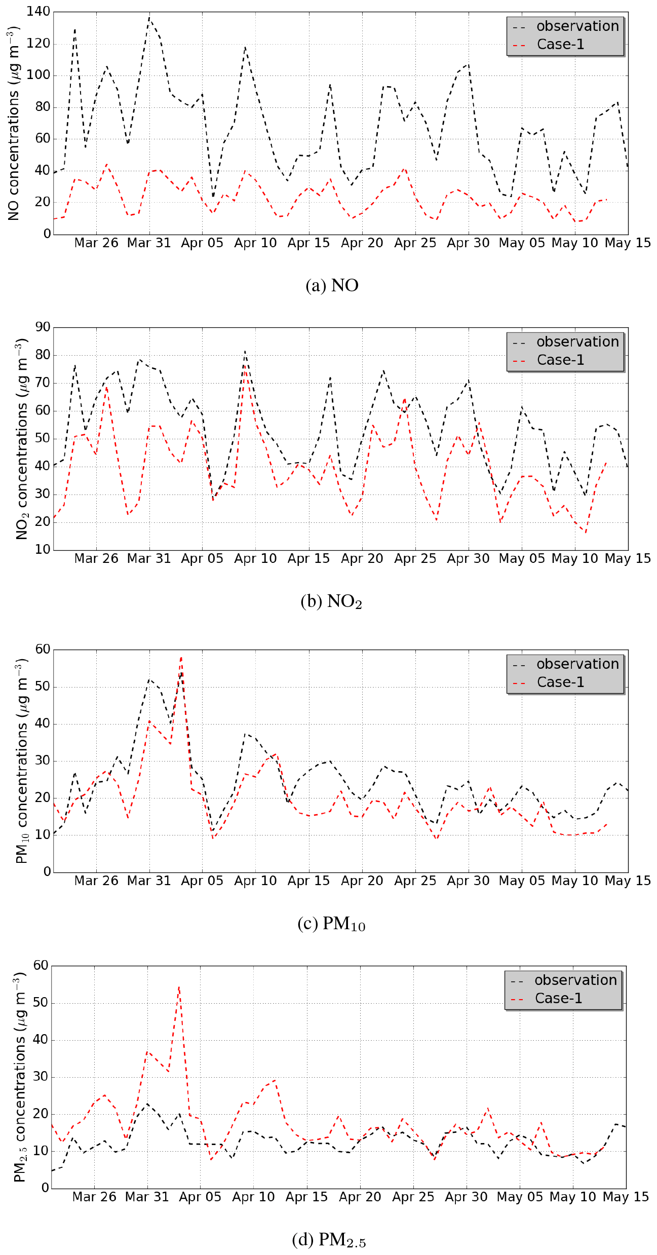
Figure 5 Comparison of daily-averaged concentrations (in µg m⁻³) in the (reference) Case-1 simulation to the measurements at the monitoring station for (a) NO, (b) NO₂, (c) PM₁₀, and (d) PM_2.5.

Table 3 Statistical indicators of the comparison of simulated hourly concentrations to the measurements at the air monitoring station.

3.2 Simulated concentrations

The reference test case (Case-1) is performed for the period from 22 March to 13 May 2014 using the options in Table 2. In Fig. 5, computed 24 h-averaged concentrations are compared to the concentrations observed at the air monitoring station operated by Airparif during the TRAFIPOLLU project.

Two distinct statistical criteria are used to evaluate the model performance for hourly concentrations: acceptance and strict criteria (Hanna and Chang, 2012; Herring and Huq, 2018), see Table 3. The corresponding statistical indicators are defined in Appendix A1.

The hourly NO₂ concentrations estimate the observations well – the acceptance criteria are validated for all statistical indicators, and the strict criteria are validated for almost all indicators: the fractional bias (FB) is equal to −31 %, while it should be lower than 30 % to satisfy the strict criteria. However, the NO concentrations are strongly underestimated and do not satisfy the acceptance criteria. These discrepancies were observed in previous studies (Kim et al., 2018; Lugon et al., 2020). The discrepancies in the simulation results obtained using MUNICH v2.0 are reduced compared to those obtained using MUNICH v1.0, but they are still high. The discrepancies can be explained by uncertainties in the traffic emission data, the vertical transfer at rooftops, and the lifetime of NO (Kim et al., 2018; Lugon et al., 2020).

The statistical indicators for the simulated PM₁₀ and PM_2.5 concentrations are also satisfactory. For PM₁₀ concentrations, both the acceptance and strict criteria are met for the different indicators. For PM_2.5 concentrations, the acceptance criteria are met by the different indicators, but the strict criteria are not met by the FB, the normalised mean square error (NMSE), and the mean geometric bias (MG). The FB is equal to 34 %, while it should be lower than 30 % to satisfy the strict criteria. The overprediction of the PM_2.5 concentrations may be due to the uncertainties in the size distribution and non-exhaust emissions. Lugon et al. (2021a) showed that the observed and simulated PM_2.5 $/$ PM₁₀ ratios are lower at traffic stations (47 % to 66 %) than at urban background stations (67 % to 76 %) because of high non-exhaust emissions, mostly emitted as coarse particles. In the reference simulation, the observed PM_2.5 $/$ PM₁₀ ratio is 51 %. However, the simulated ratio is 89 %.

Figure 6a shows the time-averaged concentrations over the simulation domain for the simulated PM_2.5 concentrations. The concentrations are high over the major streets, where the emission rates are high.

Several simulations (sensitivity test cases) are performed to estimate the influences of the different model options on the computed concentrations. In each sensitivity test case, one parameterisation or process is modified with respect to the reference simulation. The characteristics of the simulations are listed in Table 4, and the available model options are explained in Appendix B. These sensitivity test cases are presented in the following sections. The domain-averaged normalised mean error (NME) between the sensitivity test case and the reference simulation is computed: the NME is computed for each street over the whole simulation period and then averaged over the simulation domain. A larger domain-averaged NME means a larger influence of the model option tested in the sensitivity test case.

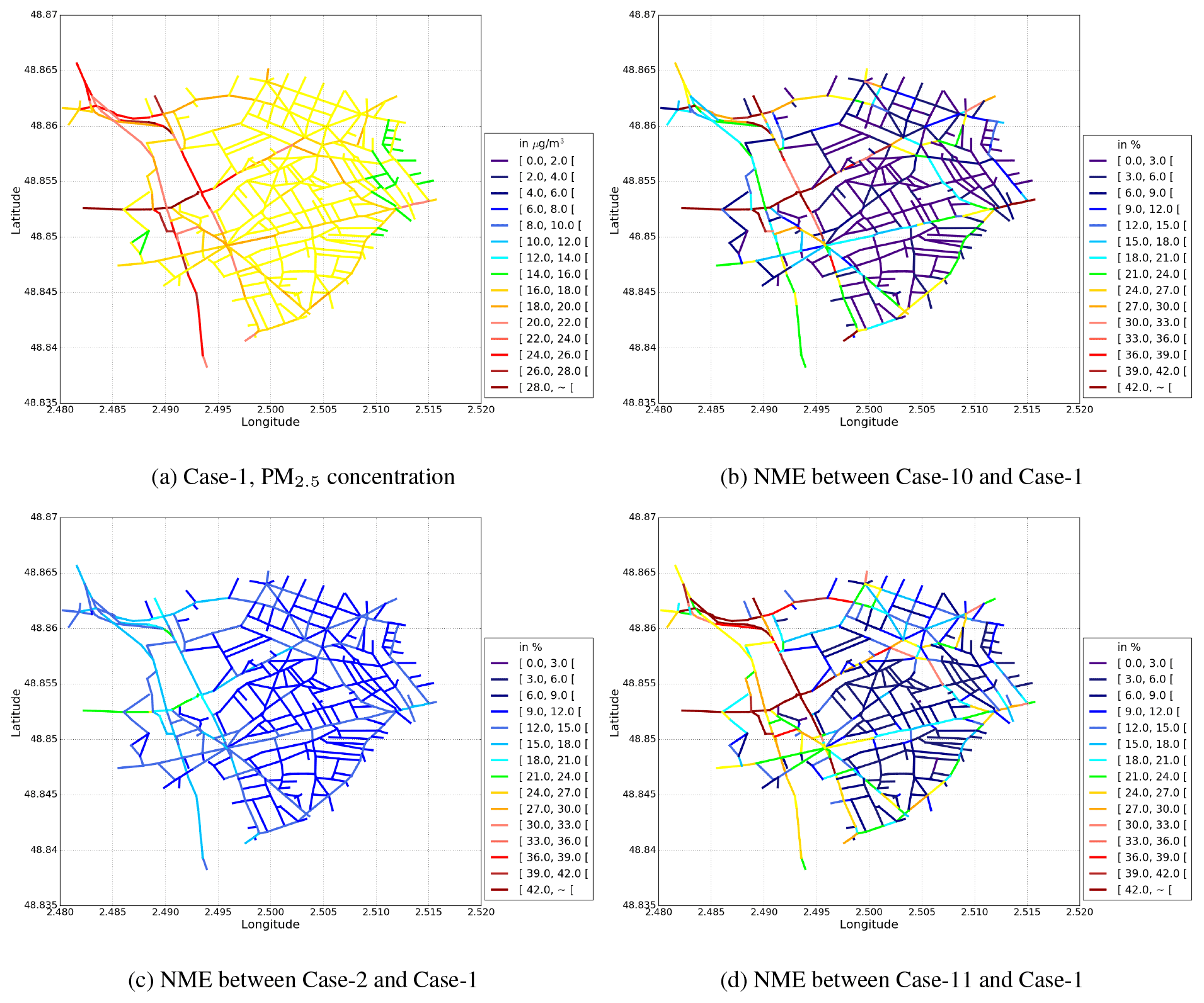
Figure 6 PM_2.5 time-averaged concentrations (in µg m⁻³) for the reference test case (Case-1, a). Normalised mean error (NME, %) between sensitivity test cases (Case-10 in b, Case-2 in c, and Case-11 in d) and the reference test case, which quantifies the average impact of parameterisations on the concentrations. The absolute differences in concentrations between the simulations are presented in additional figures in the Appendix C.

Table 4 List of test cases and normalised mean errors (NMEs, see Appendix A) between the sensitivity test cases and the reference simulation (Case-1). The NME is computed for PM_2.5 and NO₂ for each street over the whole simulation period and then averaged over the whole simulation domain.

4 Influences of parameters related to transport

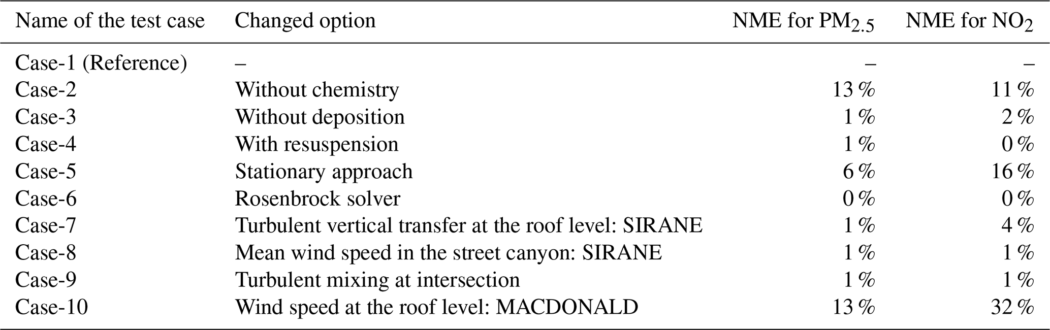
This section investigates the influences of parameters related to transport, i.e. the description of the wind velocity and the turbulence, on concentrations. Amongst the different parameterisations tested (Case-7, Case-8, Case-9, and Case-10), the estimation of the wind velocity at the roof level (Case-10) is the most influential. It directly impacts the strength of the wind speed within streets.

4.1 Wind velocity at the roof level

Two parameterisations may be used to compute the wind velocity at the roof level (u_H). In MUNICH v1.0, u_H was computed with the SIRANE parameterisation, following Soulhac et al. (2011). The MACDONALD parameterisation is added in MUNICH v2.0, as detailed in Sect. 2.2. The MACDONALD parameterisation is used in the Case-10 simulation. An increase in both NO (NME of 55 %) and NO₂ (NME of 32 %) concentrations is observed with the MACDONALD parameterisation, see Fig. 7. This increase is due to lower wind velocity at the roof level with the MACDONALD parameterisation, which leads to a lower dispersion of NO_x from the streets where the air monitoring station is located.

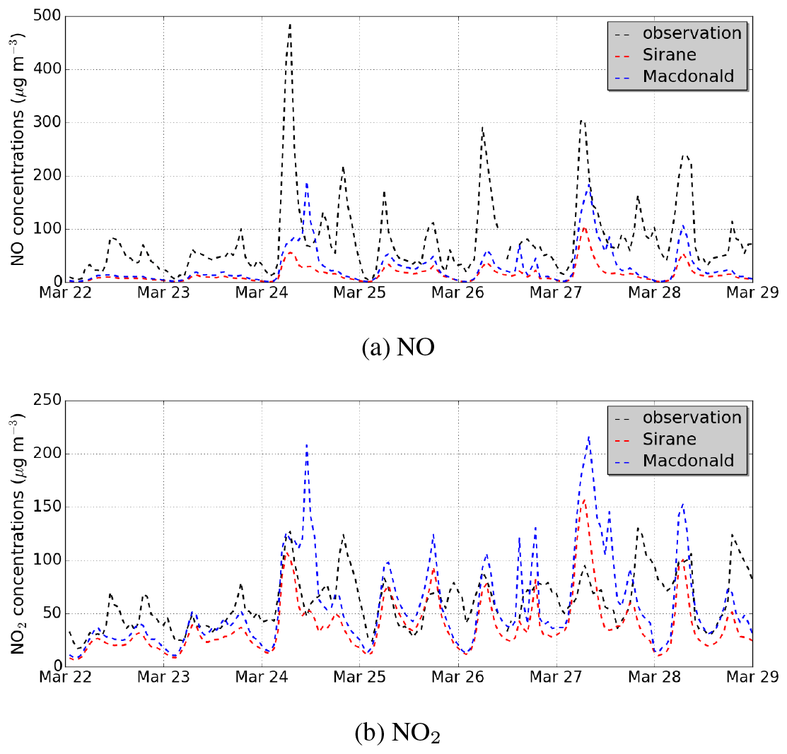
Figure 7 Comparison of observations to (a) NO and (b) NO₂ hourly concentrations (in µg m⁻³) obtained using two different parameterisations to compute the wind velocity at the roof level: SIRANE (Case-1) in red and MACDONALD (Case-10) in blue.

For the comparison with the observational data, the MACDONALD parameterisation better simulates NO concentrations than the SIRANE parameterisation does. However, the MACDONALD parameterisation overestimates the peaks of NO₂ concentrations.

Figure 6b shows the time-average NME (the NME computed on the basis of a temporal series) over different street segments of the simulation domain for the PM_2.5 concentrations. The NME is high where the concentration is high. The MACDONALD parameterisation leads to an increase of concentration at the air monitoring station with an NME of about 15 %, and the maximum NME over the street domain is about 50 % (it is 13 % over the whole domain).

Because the MACDONALD parameterisation better estimated the roof-level wind speeds than the SIRANE one, in comparison to the CFD simulation results of Maison et al. (2022), the MACDONALD parameterisation is recommended for use in MUNICH. However, because of uncertainties in the regional wind speed and friction velocity, simulations with the SIRANE parameterisation could give better scores compared to observations for some applications.

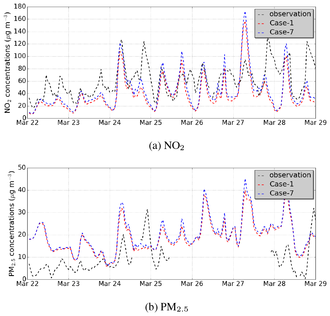
Figure 8 Comparison of observations to (a) NO₂ and (b) PM_2.5 hourly concentrations (in µg m⁻³) obtained using SCHULTE (Case-1, red line) and SIRANE (Case-7, blue line).

4.2 Turbulent transfer at the roof level

Two parameterisations are available to compute the turbulent vertical flux in MUNICH: SIRANE and SCHULTE. In the first one, the vertical flux is computed taking into account the street length and the street width. In the second one, the building height is also considered.

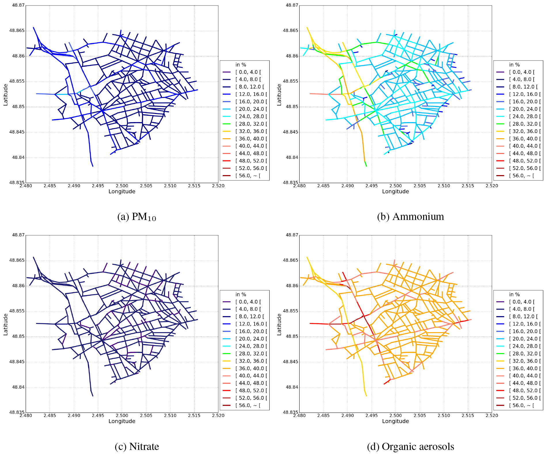
Figure 9 Temporal NME (in %) between Case-1 and Case-2 for (a) PM₁₀, (b) ammonium, (c) nitrate, and (d) organic aerosols. The absolute differences in the concentrations between the simulations are presented in additional figures in the Appendix C.

The sensitivity of the concentrations to this option is estimated by comparing the Case-7 simulation to the Case-1 simulation. Figure 8 presents a comparison of observations to NO₂ and PM_2.5 hourly concentrations in the Case-1 and Case-7 simulations. The time-averaged NME between Case-1 and Case-7, as presented in Table 4, is low (1 % for PM_2.5 and 4 % for NO₂). However, the differences between Case-1 and Case-7 are important for the peak concentrations during the morning and evening rush hours. The peak concentrations of NO₂ in the Case-7 simulation (blue line) are larger than those in the Case-1 simulation (red line) by up to 30 %. The largest differences occur on March 24 in the evening and on 28 March in the morning. The computation of the vertical flux depends on the gradient between the street concentration and the background concentration in both parameterisations. The gradient is large during the rush hours because of high traffic emissions. This large gradient leads to a large difference in the vertical flux between Case-1 and Case-7 during the rush hours. For PM_2.5, the peak concentrations are less sensitive to the parameterisation of turbulent transfer, and the maximum difference between the two cases is 13 % on 27 March in the morning. PM_2.5 concentrations are less sensitive to most parameterisations than NO₂ concentrations in our simulations except for the Case-2 simulation (see Table 4). This is due to a larger contribution of background emissions for PM_2.5 than NO₂.

Kim et al. (2018) showed that the vertical flux is higher with SCHULTE than SIRANE in areas with low buildings. On the contrary, the vertical flux is lower with SCHULTE than SIRANE in areas with tall buildings. The concentrations are then higher with the SIRANE parameterisation in the simulation domain where the building heights are low.

Because the SCHULTE parameterisation for the turbulent vertical mass transfer at roof level includes an additional dependence on the street aspect ratio compared to the SIRANE one, leading to better comparisons to the CFD simulations of Maison et al. (2022), the SCHULTE parameterisation is recommended in MUNICH.

4.3 Wind speed formulation within the street and turbulent mixing at intersections

In the Case-8 simulation, the mean wind speed in the street canyon is calculated using the SIRANE parameterisation instead of the exponential parameterisation in Case-1. Kim et al. (2018) showed that the impact of the mean speed when using the SIRANE or exponential parameterisation is low for streets of low aspect ratio (about $\mathrm{1}/\mathrm{3}$). The time-averaged NME between Case-1 and Case-8 over the street network is also low: about 1 % for PM_2.5 and 1 % for NO₂.

Soulhac et al. (2011) suggested that the turbulent mixing at intersections can be represented by considering horizontal fluctuations in the wind direction. These horizontal fluctuations are parameterised using a Gaussian distribution of the wind direction, as detailed in Appendix B. The influence of the parameterisation of the turbulent mixing at intersections is tested in the Case-9 simulation. The time-averaged NME between Case-1 and Case-9 is low: about 1 % for PM_2.5 and 1 % for NO₂.

Because the comparison to CFD simulations shows that the exponential profile overestimates the wind speed in the street, especially at the bottom of the street (Maison et al., 2022), the SIRANE parameterisation is recommended for the horizontal wind speed within the street. Taking into account horizontal fluctuations in the wind direction is not necessary because of its low influence on concentrations.

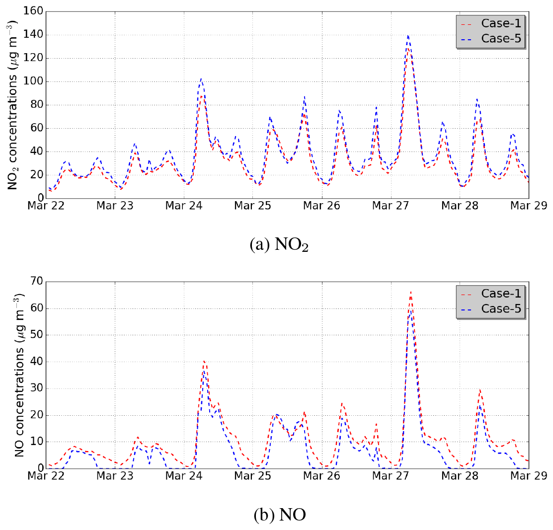
Figure 10 Comparison of (a) NO₂ and (b) NO hourly concentrations using the non-stationary approach (Case-1) in red and the stationary approach (Case-5) in blue. The concentrations are averaged over the whole simulation domain.

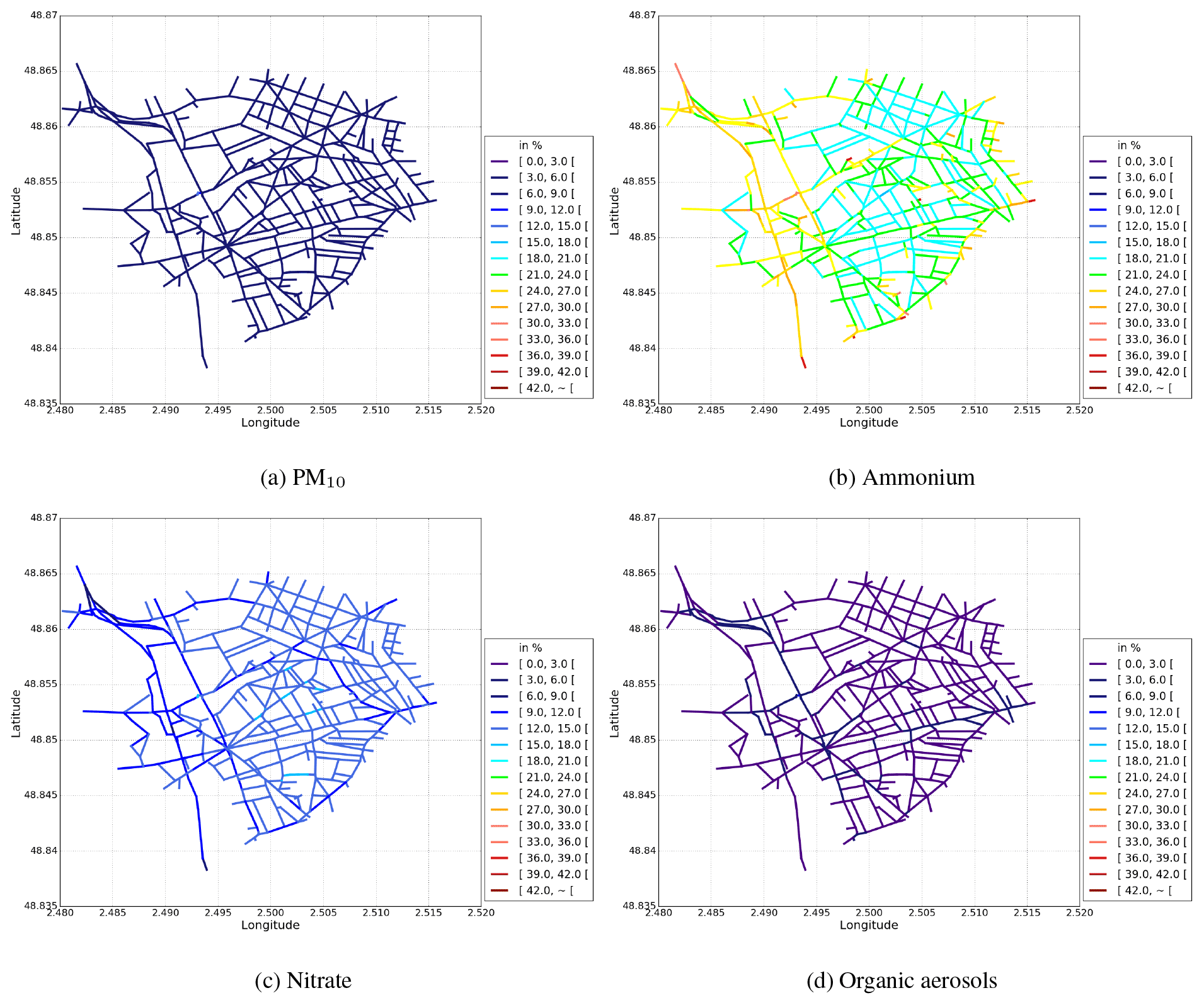
Figure 11 Temporal NME (in %) between Case-1 and Case-5 for (a) PM₁₀, (b) ammonium, (c) nitrate, and (d) organic aerosols. The absolute differences in the concentrations between the simulations are presented in additional figures in Appendix C.

5 Influences of parameters related to secondary pollutant formation

5.1 Secondary gaseous and aerosol species

In the simulation Case-2, the aerosol model SSH-aerosol is not used, and the pollutant concentrations are computed taking into account only emission, deposition, and transport processes. Figure 6c shows the time-averaged NME over the simulation domain for the PM_2.5 concentration between the Case-1 and Case-2 simulations. The NME over the whole domain for the PM_2.5 concentration is 13 %. Note that high NMEs are obtained over some major streets. Figure 9 presents the NMEs between the Case-1 and Case-2 simulations for the total PM₁₀ concentration and the concentrations of inorganic/organic aerosols. The concentrations of PM₁₀ are reduced (NME of 11 %) when the chemistry and aerosol dynamics are not modelled. The reduction is due to the absence of secondary inorganic and organic aerosol formation in simulation Case-2. Lugon et al. (2021a) showed that the average impacts of secondary aerosol formation on the PM_2.5 concentrations over the streets in Paris are 12 % for organic aerosols and 7 % for inorganic aerosols. For inorganic aerosols, the concentrations of ammonium and nitrate in Case-2 are lower (NMEs of 24 % and 5 %, respectively). A very low change in sulfate is obtained because the sulfate in the streets in mainly imported from the background (Lugon et al., 2021a). For organic aerosols, the concentrations of particles that are formed from natural sources are less reduced than those formed by human activities. It is, however, worth noting that the emission from the urban vegetation is not taken into account in this result. The NME for total organic aerosol is 43 %.

For the gas-phase species, the absence of conversion from NO to NO₂ by chemical reactions in Case-2 leads to a reduction of NO₂ in Case-2 (NME of 11 %).

As a large fraction of NO₂ is secondary, i.e. formed in the conversion of primary NO by ozone titration (Lugon et al., 2020), it is crucial to take gas-phase chemistry into account to accurately represent NO₂ concentrations. The inorganic and organic concentrations of PM are strongly influenced by aerosol dynamics, mostly because of the condensation/evaporation process (e.g. NH₃ from traffic emissions condenses with existing HNO₃). However, the coagulation process also needs to be taken into account to accurately represent the particle size distribution (Lugon et al., 2021a).

5.2 The non-stationary approach

In the simulation Case-5, the stationary hypothesis is assumed to compute the pollutant concentrations. As shown in Lugon et al. (2020) and Fig. 10, higher concentrations of NO₂ are obtained in the simulation Case-5 than in Case-1, with a temporal NME of 35 % for the Boulevard Alsace Lorraine and 16 % on average over the domain. This increase in NO₂ concentration using the stationary hypothesis may be due to more conversion from NO to NO₂; the NO_x concentration is similar in Case-1 and Case-5, and the time-averaged NME is lower than 1 %. Figure 11 presents the time-averaged NME in the concentrations simulated between Case-5 and Case-1. For PM₁₀ and PM_2.5, the time-averaged NME is not as high as for NO₂. The NME is about 5 % for both PM₁₀ and PM_2.5 on average over the domain.

For inorganic aerosols, ammonium concentrations are larger (NME of 24 %) when using the stationary approach than when using the non-stationary approach. The concentration of nitrate in Case-5 is lower (NME of 13 %). For organic aerosols, the differences are low (NME of 3 %).

In Case-6, the Rosenbrock rather than the ETR solver is used in the non-stationary approach. The simulated concentrations are not sensitive to the solver used (the time-averaged NME is less than 1 %).

For secondary compounds, such as NO₂ and inorganic and organic aerosols, it is crucial to use the non-stationary approach, as it ensures numerical stability and strongly affects the concentrations.

6 Parameters related to deposition and resuspension

In the Case-3 simulation, deposition is not taken into account. Very low differences are obtained between the Case-1 and Case-3 simulations.

Particle dry deposition has a negligible impact on PM concentration over the simulation domain (the time-averaged NME is 1 % for PM_2.5, see Table 4). The gas-phase deposition parameterisation also has a low impact on sulfur dioxide (SO₂) and ozone (O₃) concentrations (the NME is about 1 % on average). It is, however, important to note that this conclusion does not take into account the potential role of urban vegetation in the deposition process (Janhäll, 2015). Moreover, the average building height in the considered district is rather low. The deposition process could have a more significant impact on a more densely built urban area.

In the Case-4 simulation, parameterisation for particle resuspension is used. The amount of resuspended mass in MUNICH is limited by the deposited mass (Lugon et al., 2021b). Because the deposited mass is not significant in Case-3, the resuspended mass in Case-4 is also low.

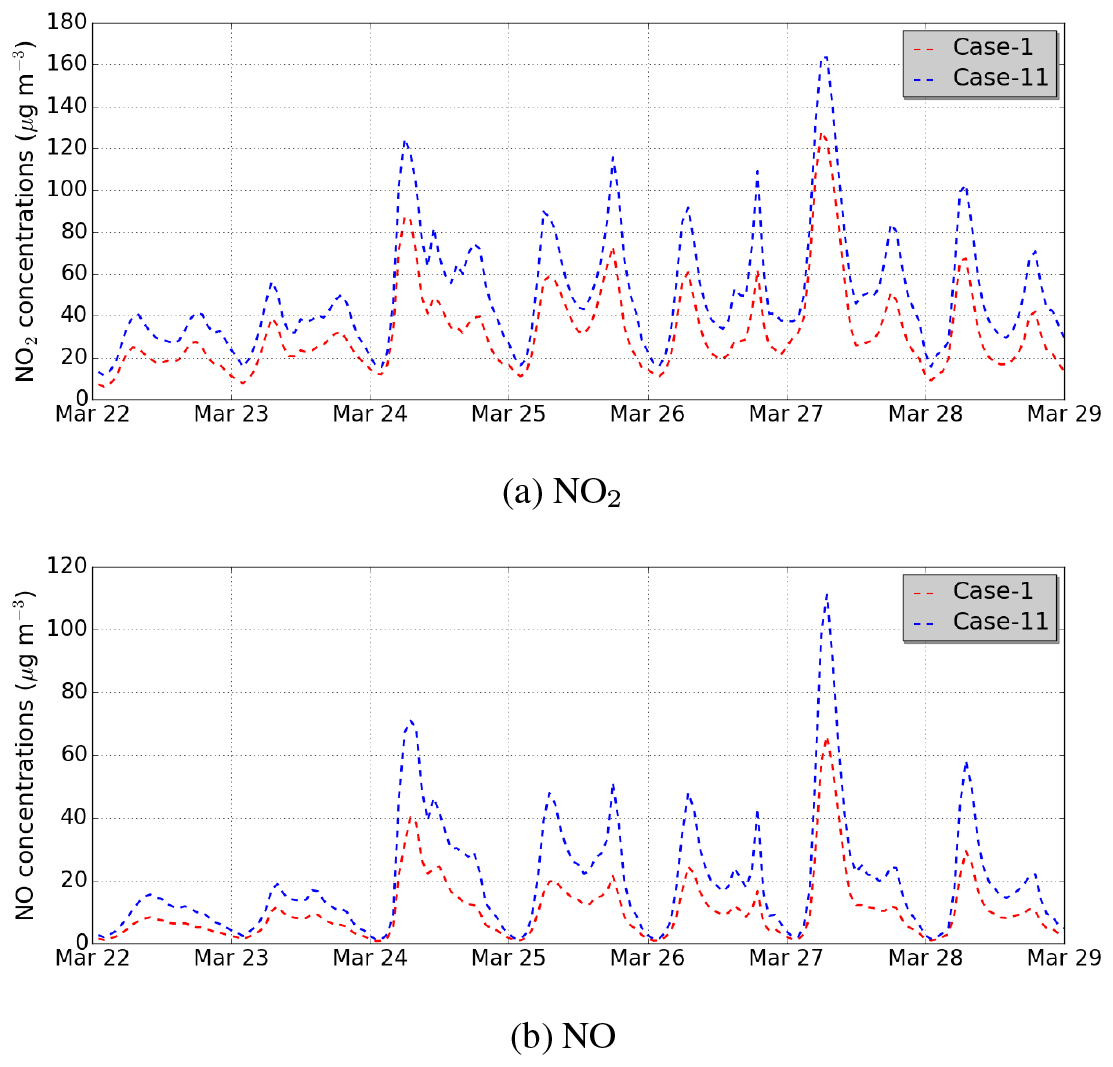
Figure 12 Comparison of the Case-1 hourly concentrations to those in the sensitivity simulation Case-11 (which modifies the building aspect ratio over the whole simulation domain): (a) NO₂ and (b) NO.

Dry deposition on urban surfaces and resuspension have a low impact on concentrations in Paris. However, wet deposition by rain may have a large impact during rainy days and should be considered (Roustan et al., 2010; Vivanco et al., 2018).

7 Sensitivity simulations

The street concentrations are strongly influenced by the building characteristics and by the traffic in the streets. To illustrate these influences, two sensitivity simulations are performed by arbitrarily modifying the building aspect ratio and by suppressing the traffic in a street.

7.1 Influence of the building aspect ratio

The building aspect ratio, which is the ratio of building height to street width (H/W), is an important characteristic of streets because it influences the turbulent transfer of pollutants at roof level and the vertical wind profile in the streets (Kim et al., 2018).

An additional sensitivity simulation (Case-11) is conducted to estimate the effect of the aspect ratio. The Case-1 reference simulation is repeated by artificially modifying the building height and the street width. The street width is reduced by a factor of $\sqrt{\mathrm{3}}$ and the building height is increased by a factor of $\sqrt{\mathrm{3}}$ for all street segments. Therefore, the aspect ratio is increased by a factor of 3. Modifying both the building height and the street width in this way is important, as it means that the volume of the street segments is not changed. Figure 6d shows that the NME between the Case-1 and Case-11 simulations is high where the PM_2.5 concentration is high. Figure 12 shows the temporal variations of the NO and NO₂ concentrations, which are averaged over the whole simulation domain (Case-1 and Case-11 simulations). The concentrations of NO and NO₂ in the Case-11 simulation are larger than those in the Case-1 simulation by NMEs of 72 % and 44 %, respectively. The concentrations of PM_2.5 and PM₁₀ also increase in the Case-11 simulation, with NMEs of 16 % and 17 %, respectively. These larger concentrations are due to reduced turbulent transfer at roof level and reduced mean horizontal wind speeds. Kim et al. (2018) estimated that the turbulent transfer decreases by 30 % when the aspect ratio increases by a factor of 2.

7.2 Effects of streets without cars

Many European cities have taken low-emission zone (LEZ) measures to reduce street-level air pollution. The effects of this type of measure can be simulated by reducing emissions in specific streets. An additional sensitivity simulation (Case-12) is conducted to estimate the effects of emission reduction in a street. In the Case-12 simulation, the setup for the reference simulation (Case-1) is used, but the emissions are set to zero in the Boulevard Alsace Lorraine (see Fig. 4). This means that all vehicles are forbidden on this street. The background concentrations are the same in Case-12 as in the reference simulation, meaning that the total emissions are the same in both simulations. However, we assume that traffic is redistributed in streets near to, but not directly adjacent to, the Boulevard Alsace Lorraine.

Figure 13 shows the differences in NO₂ concentrations between the Case-1 and Case-12 simulations. The NO₂ concentration in Boulevard Alsace Lorraine in the Case-12 simulation is lower than that in the Case-1 simulation by 43 % (Case-1: 44 µg m⁻³ vs. Case-12: 25 µg m⁻³). This shows that pollutant concentrations are not negligible, even though they are not emitted in the street. This is due to the pollutant transfer from the overlying atmosphere and from the neighboring streets. However, the concentrations are strongly reduced. For PM₁₀ and PM_2.5, the reduction is lower than for NO₂ (18 % for PM₁₀ and 16 % for PM_2.5). This higher contribution of street emissions to NO₂ than to PM concentrations is due to differences in the atmospheric processes leading to PM and NO₂ concentrations (longer atmospheric lifetimes and, therefore, larger contributions of the background, leading to lower contributions of local PM emissions).

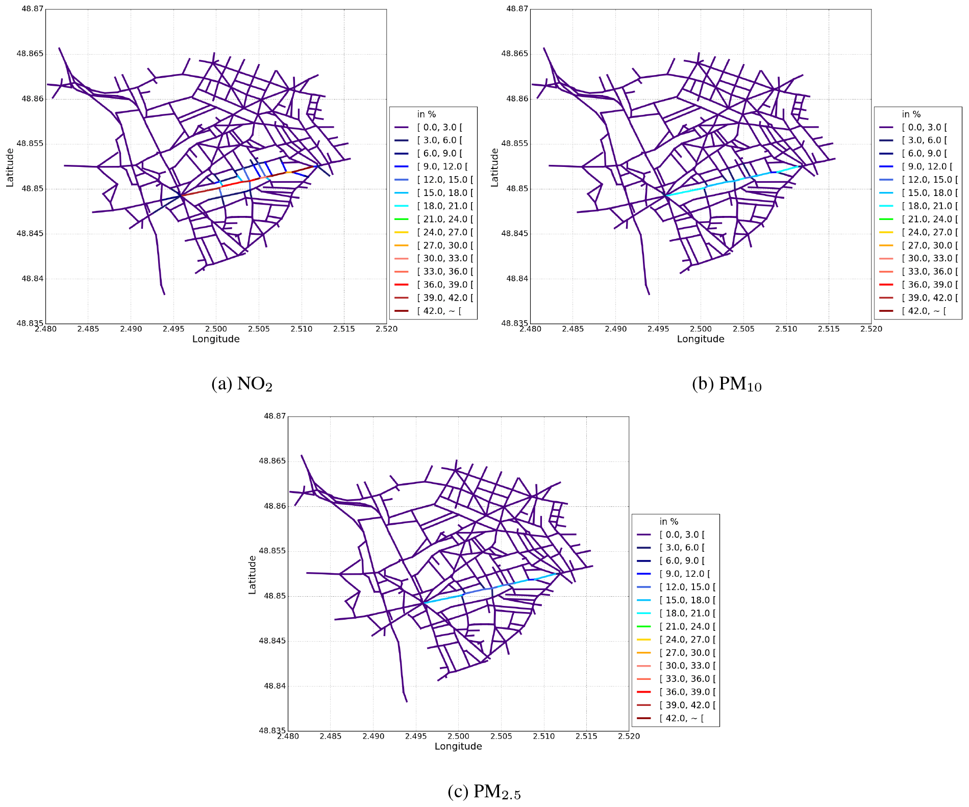
Figure 13 Temporal NME (in %) between Case-1 and Case-12 for (a) NO₂, (b) PM₁₀, and (c) PM_2.5. The absolute differences in the concentrations between the simulations are presented in additional figures in Appendix C.

8 Conclusions

The street-network model MUNICH v2.0 for multi-pollutant modelling in street canyons has been presented. A reference test case was set up for the east side of Greater Paris, where measurements were performed. NO₂, PM_2.5, and PM₁₀ are well modelled with MUNICH v2.0 compared to measurements.

A new parameterisation to compute the wind velocity at the roof level led to an increase in PM_2.5 (13 %) and NO₂ (32 %) concentrations at the air monitoring station near traffic. The turbulent vertical transfer increases when the parameterisation takes into account the building height. This is due to low building heights in the street network studied here. This high sensitivity to wind velocity at the roof level underlines the importance of meteorological downscaling to accurately represent the transition from the regional to the street scale.

The SSH-aerosol model is implemented in MUNICH v2.0 for primary and secondary aerosol modelling in street canyons, taking into account gaseous chemistry leading to the formation of condensables, condensation/evaporation, nucleation, and coagulation. The PM₁₀ and PM_2.5 concentrations increase by 11 % and 13 %, respectively, if SSH-aerosol is used. This increase is due to the formation of secondary inorganic and organic aerosols. The NO₂ concentration increases by 11 % when using SSH-aerosol. A non-stationary approach was developed to model reactive pollutants. On average, over the street network considered, the non-stationary approach leads to a decrease in NO₂ concentration of 16 % compared to the stationary approach.

In contrast to MUNICH v1.0, parameterisations of particle deposition and resuspension are also added in MUNICH v2.0. However, their impact on pollutant concentrations in the street canyons is low for the considered domain.

MUNICH may be easily used with background concentrations from a regional air-quality model in a one-way coupling approach. For the next step, the coupling between MUNICH v2.0 and the regional air-quality model will be improved by considering two-way coupling. The coupled model will be an updated version of the street-in-grid model, which computes both the pollutant concentrations within the street network and the average concentrations for the overlying atmosphere grid at the same time.

Appendix A: Statistical indicators

Table A1 Definitions of the statistical indicators.

c_i: modeled values, o_i: observed values, n: number of data.
$\stackrel{\mathrm{‾}}{o}=\frac{\mathrm{1}}{n}\sum _{i=\mathrm{1}}^n{o}_i$ and $\stackrel{\mathrm{‾}}{c}=\frac{\mathrm{1}}{n}\sum _{i=\mathrm{1}}^n{c}_i$

Appendix B: Modelling options in MUNICH

Several modelling options are available in MUNICH in order to handle the complexity and the computational time.

The options related to the modelling of the pollutant transport, deposition, and resuspension are detailed here. Note that the options linked to the modelling of chemical transformations and aerosol dynamics are presented in the article describing the SSH-aerosol model (Sartelet et al., 2020).

First of all, it is useful to present the main equations solved in MUNICH before the presentation of the options.

The time variation of the mass M $\frac{\mathrm{d}M}{\mathrm{d}t}$ is computed using a transport-related term ($\frac{\mathrm{d}M}{\mathrm{d}t}{|}_{\mathrm{transp}}$) and a chemistry-related term ($\frac{\mathrm{d}M}{\mathrm{d}t}{|}_{\mathrm{chem}}$):

$$\begin{array}{}\text{(B1)}& {\displaystyle \frac{\mathrm{d}M}{\mathrm{d}t}}={\displaystyle \frac{\mathrm{d}M}{\mathrm{d}t}}{|}_{\mathrm{transp}}+{\displaystyle \frac{\mathrm{d}M}{\mathrm{d}t}}{|}_{\mathrm{chem}}.\end{array}$$

The transport-related term is computed as

$$\begin{array}{}\text{(B2)}& {\displaystyle \frac{\mathrm{d}M}{\mathrm{d}t}}{|}_{\mathrm{transp}}=Q_{\mathrm{inflow}}+Q_{\mathrm{emis}}-(Q_{\mathrm{outflow}}+Q_{\mathrm{vert}}+Q_{\mathrm{dep}}),\end{array}$$

where Q_inflow is the incoming flux to the street, Q_emis is the emission flux in the street, Q_outflow is the outgoing flux from the street, Q_vert is the vertical exchange flux at the roof level, and Q_dep is the deposition flux.

• With_stationary_hypothesis :
  whether the stationary hypothesis is assumed or not (available options: yes or no)

  If the stationary approach is used, the concentrations are computed in each street segment by assuming that $\frac{\mathrm{d}M}{\mathrm{d}t}{|}_{\mathrm{transp}}=\mathrm{0}$. The non-stationary approach is recommended to model reactive species/pollutants. Note that the computation time increases by a factor of 3 when using the non-stationary approach for the reference test case (see Sect. 2.3 and also Sect. 5.2).

• Numerical_method_parameterisation :
  numerical solver (available options: ETR or Rosenbrock) The solver used to solve Eq. (B2) with the non-stationary approach may either be the Explicit Trapezoidale Rule (ETR) or Rosenbrock. If the ETR solver is used, Eq. (B2) is discretised as Lugon et al. (2020)

  $$\begin{array}{}\text{(B3)}& {\displaystyle }{C}_s^{n+\mathrm{1}}& {\displaystyle }=C_s^n+{\displaystyle \frac{\mathrm{\Delta }t}{\mathrm{2}}}\left(F\right(C_s^n)+F(C_s^{*}\left)\right)\text{(B4)}& {\displaystyle }{C}_s^{*}& {\displaystyle }=C_s^n+\mathrm{\Delta }tF\left(C_s^n\right),\end{array}$$

  where s represents a chemical species (gas or particle), $C_s^n$ is the concentration at time tⁿ, and $F\left(C_s^n\right)$ represents the time derivative of $C_s^n$ due to transport-related processes obtained by Eq. (B2). The time step Δt is adjusted by

  $$\begin{array}{}\text{(B5)}& \mathrm{\Delta }{t}^{n+\mathrm{1}}=\mathrm{\Delta }{t}^n\sqrt{{\displaystyle \frac{{\mathrm{\Delta }}_{\mathrm{0}}}{{\mathrm{\Delta }}_{\mathrm{1}}}}},\end{array}$$

  where Δ₁ is the relative error and Δ₀ is the relative error precision, which is set to 0.01. The relative error Δ₁ is computed as

  $$\begin{array}{}\text{(B6)}& {\mathrm{\Delta }}_{\mathrm{1}}=\left|\right|{\displaystyle \frac{{\mathit{C}}^{n+\mathrm{1}}-{\mathit{C}}^{*}}{{\mathit{C}}^{n+\mathrm{1}}}}|{|}_{\mathrm{2}},\end{array}$$

  where C is the vector of the concentrations of all chemical species. The Euclidean norm is used to compute the relative error so that the error for all species is averaged.

  The Rosenbrock solver is implemented to improve the numerical stability of the non-stationary approach:

  $$\begin{array}{}\text{(B7)}& C_s^{n+\mathrm{1}}=C_s^n+{\displaystyle \frac{\mathrm{3}}{\mathrm{2}}}\mathrm{\Delta }t{k}_{\mathrm{1}}+{\displaystyle \frac{\mathrm{1}}{\mathrm{2}}}\mathrm{\Delta }t{k}_{\mathrm{2}}.\end{array}$$

  k₁ and k₂ are computed as

  $$\begin{array}{}\text{(B8)}& {\displaystyle }(\mathrm{1}-\mathit{\gamma }\mathrm{\Delta }t\mathbf{J})k_{\mathrm{1}}& {\displaystyle }=F\left(C_s^n\right)\text{(B9)}& {\displaystyle }(\mathrm{1}-\mathit{\gamma }\mathrm{\Delta }t\mathbf{J})k_{\mathrm{2}}& {\displaystyle }=F(C_s^{n+\mathrm{1}}+\mathit{\gamma }{k}_{\mathrm{1}})-\mathrm{2}{k}_{\mathrm{1}},\end{array}$$

  where γ is $\mathrm{1}+\sqrt{\mathrm{2}}/\mathrm{2}$ and J is a Jacobian matrix of Eq. (B2).

• Transfer_parameterisation :
  parameterisation to compute the turbulent vertical mass transfer (available options: SIRANE or SCHULTE)

  The vertical flux, Q_vert, is formulated using the SIRANE option as follows:

  $$\begin{array}{}\text{(B10)}& Q_{\mathrm{vert}}={\displaystyle \frac{{\mathit{\sigma }}_{\mathrm{W}}WL}{\sqrt{\mathrm{2}}\mathit{\pi }}}\left(C_{\mathrm{street}}-C_{\mathrm{background}}\right),\end{array}$$

  where C_background is the mean concentration above the street segment, L is the street length, and σ_W is the standard deviation of the vertical wind velocity at roof level, which depends on atmospheric stability.

  Using the SCHULTE option, the street aspect ratio (a_r, the ratio of building height to street width) is taken into account:

  $$\begin{array}{}\text{(B11)}& \begin{array}{rl}{Q}_{\mathrm{vert}}& =\mathrm{0.45}{\mathit{\sigma }}_{\mathrm{W}}WL\left({\displaystyle \frac{\mathrm{1}}{\mathrm{1}+a_{\mathrm{r}}}}\right)\\ & \left(C_{\mathrm{street}}-C_{\mathrm{background}}\right),\end{array}\end{array}$$

  where $a_{\mathrm{r}}=H/W$.

• Building_height_wind_speed_ parameterisation :
  parameterisation to compute wind speed at the roof level (available options: SIRANE or MACDONALD)

  Using the SIRANE option (Soulhac et al., 2008), the wind speed at the roof level and at the centre of the street (u_M) is computed as

  $$\begin{array}{}\text{(B12)}& u_M=u_{*}\sqrt{{\displaystyle \frac{\mathit{\pi }}{\sqrt{\mathrm{2}}{\mathit{\kappa }}^{\mathrm{2}}C}}\left(Y_{\mathrm{0}}\right(C)-{\displaystyle \frac{J_{\mathrm{0}}\left(C\right)Y_{\mathrm{1}}\left(C\right)}{J_{\mathrm{1}}\left(C\right)}})},\end{array}$$

  where u_* is the friction velocity and J₀, J₁, and Y₁ are Bessel functions. κ is the von Kármán constant. To compute the mean wind speed at the roof level over the street width (u_H), the horizontal wind speed variation of Soulhac et al. (2008) is considered. As discussed in Sect. 2.2, using the MACDONALD option, the wind speed at the roof level (u_H) is computed as

  $$\begin{array}{}\text{(B13)}& u_H={\displaystyle \frac{u_{*}}{\mathit{\kappa }}}\ln \left({\displaystyle \frac{H-d_{\mathrm{c}}}{z_{\mathrm{0}\mathrm{c}}}}\right)=u_{\mathrm{ref}}\times {\displaystyle \frac{\ln \left(\frac{H-d_{\mathrm{c}}}{z_{\mathrm{0}\mathrm{c}}}\right)}{\ln \left(\frac{z_{\mathrm{ref}}-d_{\mathrm{c}}}{z_{\mathrm{0}\mathrm{c}}}\right)}}.\end{array}$$

• Mean_wind_speed_parameterisation :
  parameterisation to compute the mean wind speed within the street canyon (available options: exponential or SIRANE)

  Using the exponential option (Lemonsu et al., 2004), the wind speed within the street canyon is computed as

  $$\begin{array}{}\text{(B14)}& u_{\mathrm{street}}=u_H\left|\cos \left(\mathit{\phi }\right)\right|{\displaystyle \frac{\mathrm{2}}{a_{\mathrm{r}}}}\left(\mathrm{1}-\exp \left({\displaystyle \frac{a_{\mathrm{r}}}{\mathrm{2}}}\left({\displaystyle \frac{z_{\mathrm{0}}}{H}}-\mathrm{1}\right)\right)\right),\end{array}$$

  where u_H represents the wind speed at the roof level, which is computed by the option detailed above (see Sect. 2.2); φ is the angle between the street orientation and the wind direction; and z₀ is the aerodynamic roughness of canyon surfaces.

  Using the SIRANE option (Eq. 1 in Soulhac et al., 2011), the wind speed within the street canyon is computed as

  $$\begin{array}{}\text{(B15)}& \begin{array}{rl}{u}_{\mathrm{street}}& =u_M\left|\cos \left(\mathit{\phi }\right)\right|{\displaystyle \frac{{\mathit{\delta }}_i^{\mathrm{2}}}{HW}}\left({\displaystyle \frac{\mathrm{2}\sqrt{\mathrm{2}}}{C}}(\mathrm{1}-\mathit{\beta })\right.\\ & \left(\mathrm{1}-{\displaystyle \frac{C^{\mathrm{2}}}{\mathrm{3}}}+{\displaystyle \frac{C^{\mathrm{4}}}{\mathrm{45}}}\right)+\mathit{\beta }{\displaystyle \frac{\mathrm{2}\mathit{\alpha }-\mathrm{3}}{\mathit{\alpha }}}\\ & \left.+\left({\displaystyle \frac{W}{{\mathit{\delta }}_i}}-\mathrm{2}\right){\displaystyle \frac{\mathit{\alpha }-\mathrm{1}}{\mathit{\alpha }}}\right),\end{array}\end{array}$$

  where ${\mathit{\delta }}_i=min(H,W/\mathrm{2})$, $\mathit{\alpha }=ln\frac{{\mathit{\delta }}_i}{z_{\mathrm{0}}}$, $\mathit{\beta }=\exp \left(\frac{C}{\sqrt{\mathrm{2}}}\left(\mathrm{1}-\frac{H}{{\mathit{\delta }}_i}\right)\right)$, and C is a solution of $\frac{z_{\mathrm{0}}}{{\mathit{\delta }}_i}=\frac{\mathrm{2}}{C}\exp \left(\frac{\mathit{\pi }}{\mathrm{2}}\frac{Y_{\mathrm{1}}\left(C\right)}{J_{\mathrm{1}}\left(C\right)}-\mathrm{0.577}\right)$.

• With_horizontal_fluctuation :
  whether turbulent mixing at intersection via the horizontal fluctuation of the wind direction is taken into account or not (available options: yes or no)

  The horizontal fluctuation of the wind direction represents the turbulent mixing of the air across the intersection (Soulhac et al., 2008). The fluctuation is computed by the following steps:

  • 1.

    When the fluctuation is not taken into account, compute the air flux from street i to street j, P_i,j, for wind direction φ using the outgoing flux and the incoming flux at Eq. (B2).

  • 2.

    Perform N computations of the air flux $P_{i,j}(\mathit{\phi }+\mathit{\sigma })$ for the wind direction φ+σ, where σ is the fluctuation of the wind direction (which ranges from −20 to 20^∘) and N is the number of σ values (N is 10 when σ is 20^∘).

  • 3.

    Compute the sum of the air flux.

  $$\begin{array}{}\text{(B16)}& P_{i,j}=\sum f\left(\mathit{\sigma }\right)P_{i,j}(\mathit{\phi }+\mathit{\sigma }),\end{array}$$

  where f(σ) is a Gaussian distribution of the wind direction, ranging from 0 to 1.

• Deposition_wind_profile :
  wind profile option for dry deposition (available options: MASSON or MACDONALD)

  The friction velocity is used to compute the deposition as follows:

  $$\begin{array}{}\text{(B17)}& u_{*}=\mathit{\kappa }\exp \left(p({\displaystyle \frac{z}{h}}-\mathrm{1})/\log (z/z_{\mathrm{0}})\right),\end{array}$$

  where p is the parameter for the wind profile.

  The parameter p may be computed using the MASSON option:

  $$\begin{array}{}\text{(B18)}& p=\mathrm{0.5}{\displaystyle \frac{H}{W}},\end{array}$$

  or using the MACDONALD option:

  $$\begin{array}{}\text{(B19)}& p=\mathrm{9.6}{\mathit{\lambda }}_f,\end{array}$$

  where ${\mathit{\lambda }}_f=\frac{H}{W+\frac{{\mathit{\lambda }}_{p}W}{\mathrm{1}-{\mathit{\lambda }}_p}}$ and λ_p is the building density.

• Particles_dry_velocity_option :
  parameterisation for aerosol deposition (available options: Zhang, Giardina, Venkatram, or Muyshondt)

  Using the Zhang option (Zhang et al., 2001), the deposition velocity is computed as

  $$\begin{array}{}\text{(B20)}& v_{\mathrm{d}}=v_{\mathrm{s}}+{\displaystyle \frac{\mathrm{1}}{R_{\mathrm{street}}}},\end{array}$$

  where R_street is the total resistance due to the aerodynamic resistance of the street and the surface resistance, and v_s is the sedimentation velocity.

  Using the Giardina option (Giardina and Buffa, 2018), the deposition velocity is computed as

  $$\begin{array}{}\text{(B21)}& v_{\mathrm{d}}=v_{\mathrm{s}}/(\mathrm{1}-{\exp }^{v_{\mathrm{s}}({\mathrm{Ra}}_{\mathrm{street}}+\frac{\mathrm{1}}{R_{\mathrm{eq}}})}),\end{array}$$

  where Ra_street is the total aerodynamic resistance of the street and R_eq represents the resistance due to Brownian diffusion.

  Using the Venkatram option (Venkatram and Pleim, 1999), the deposition velocity is computed as

  $$\begin{array}{}\text{(B22)}& v_{\mathrm{d}}=v_{\mathrm{s}}/(\mathrm{1}-{\exp }^{v_{\mathrm{s}}{R}_{\mathrm{street}}}).\end{array}$$

  Using the Muyshondt option (Muyshondt et al., 1996), the deposition velocity is computed as

  $$\begin{array}{}\text{(B23)}& v_{\mathrm{d}}=v_{\mathrm{s}}+v_{Re},\end{array}$$

  where v_Re represents the influence of the Reynolds number on the deposition velocity.

  Dry deposition on urban surfaces and resuspension have a low impact on concentrations in Paris. However, wet deposition by rain may have a large impact during rainy days, and should be considered (Roustan et al., 2010; Vivanco et al., 2018).

• With_resuspension :
  whether the resuspension is taken into account or not (available options: yes or no)

  Particle resuspension is computed based on the resuspension factor f_res:

  $$\begin{array}{}\text{(B24)}& f_{\mathrm{res}}=\sum _{v=\mathrm{1}}^{\mathrm{2}}{N}_v\left({\displaystyle \frac{u_v}{u_{\mathrm{ref}}\left(r\right)}}\right)f_{\mathrm{0},v},\end{array}$$

  where v indicates the vehicle type, N_v is the vehicle flow (vehicles per hour), u_v is the vehicle speed (km h⁻¹), u_ref(r) is the reference vehicle speed for the resuspension process (km h⁻¹), and f_0,v is the reference mass fraction of the resuspension process (per vehicle). This is detailed in Lugon et al. (2021b).

• With_drainage_aerosol :
  whether drainage is taken into account or not (available options: yes or no)

  $$\begin{array}{}\text{(B25)}& f_{\mathrm{wash}}={\displaystyle \frac{\mathrm{1}}{\mathit{\delta }t}}\left(\mathrm{1}-\exp \left(-h_{\mathrm{drain},\mathrm{eff}}{\displaystyle \frac{g_{\mathrm{road}}-g_{\mathrm{road},\min }}{g_{\mathrm{road},\min }}}\right)\right),\end{array}$$

  where δt is the time, h_drain,eff is the drainage efficiency parameter, g_road is the amount of water present on the street surface (mm), and g_road,min is the minimum water content for the drainage process (mm).

  When this option is used, the wash-off factors are computed and associated with the precipitation. This is detailed in Lugon et al. (2021b).

• With_chemistry :
  whether chemistry is taken into account or not (available options: yes or no)

  The SSH-aerosol model is used when this option is set to yes. The options for the chemistry model are defined in the namelist of SSH-aerosol, namelist.ssh.

Appendix C: Absolute differences in the concentrations

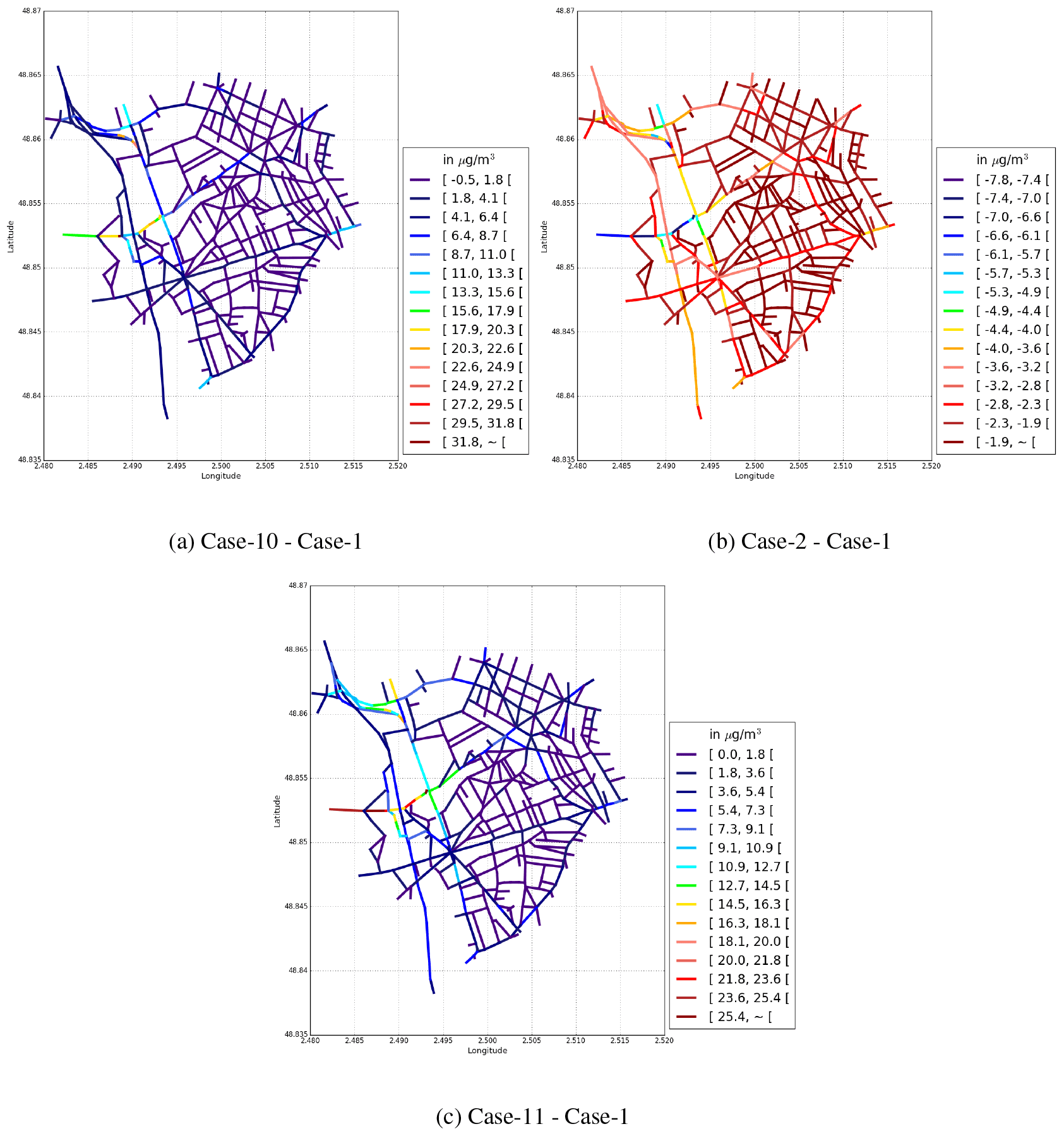
Figure C1 Differences in time-averaged PM_2.5 concentrations (in µg m⁻³) between the reference test case (Case-1) and a sensitivity test case.

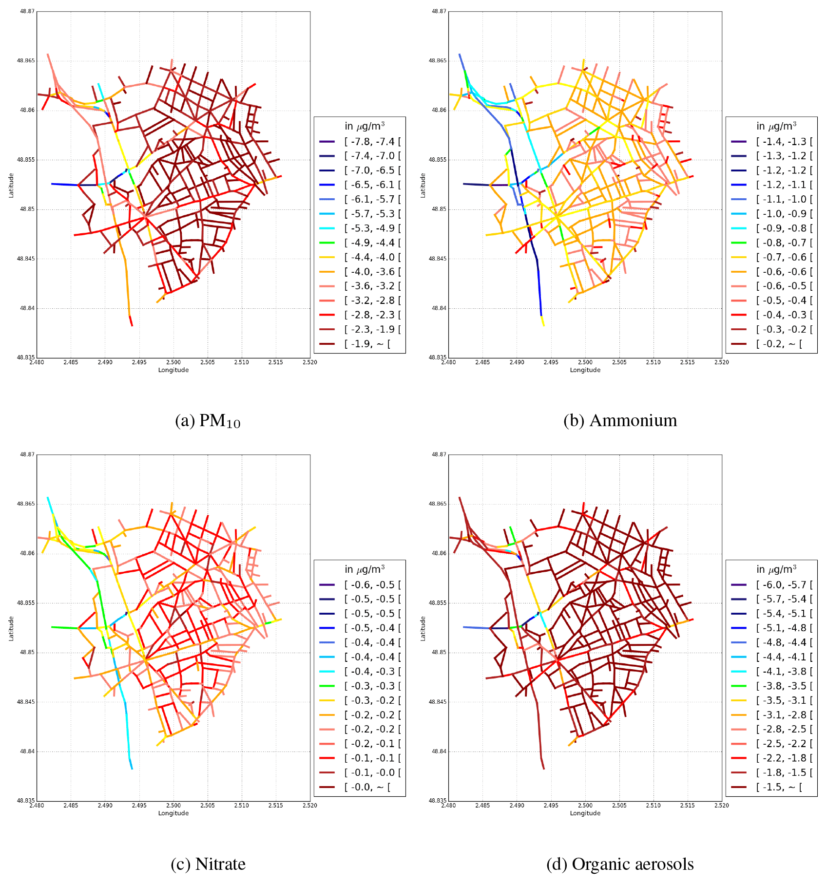
Figure C2 Differences in time-averaged concentrations (in µg m⁻³) between Case-2 and Case-1 (Case-2 − Case-1) for (a) PM₁₀, (b) ammonium, (c) nitrate, and (d) organic aerosols.

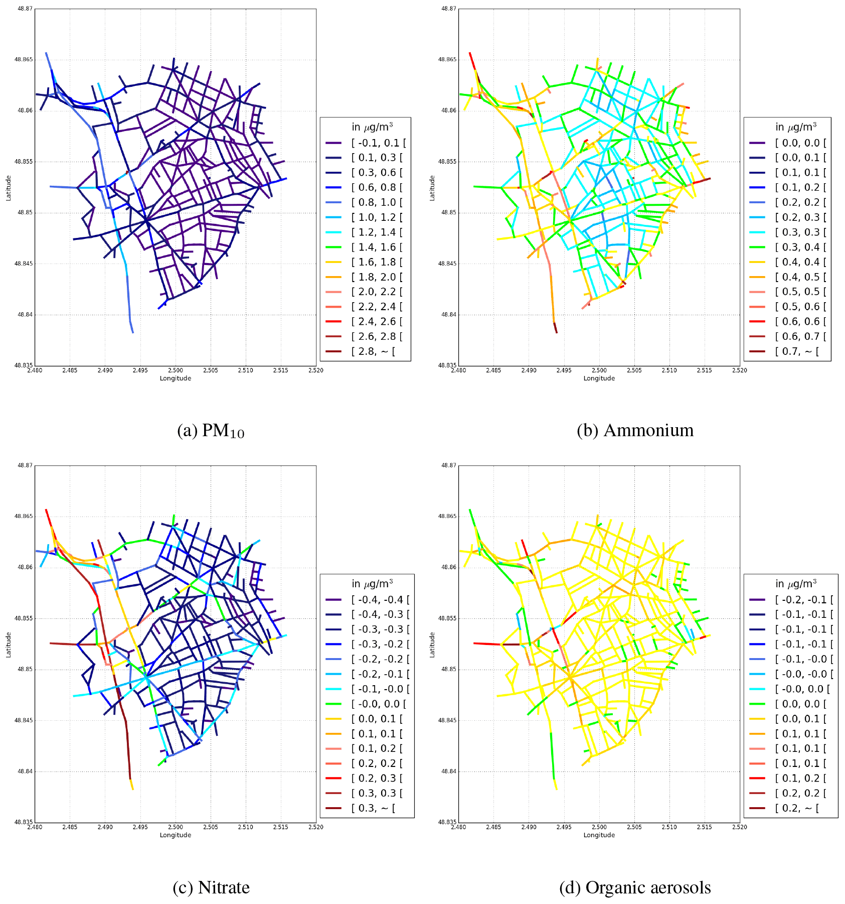
Figure C3 Differences in time-averaged concentrations (in µg m⁻³) between Case-5 and Case-1 (Case-5 − Case-1) for (a) PM₁₀, (b) ammonium, (c) nitrate, and (d) organic aerosols.

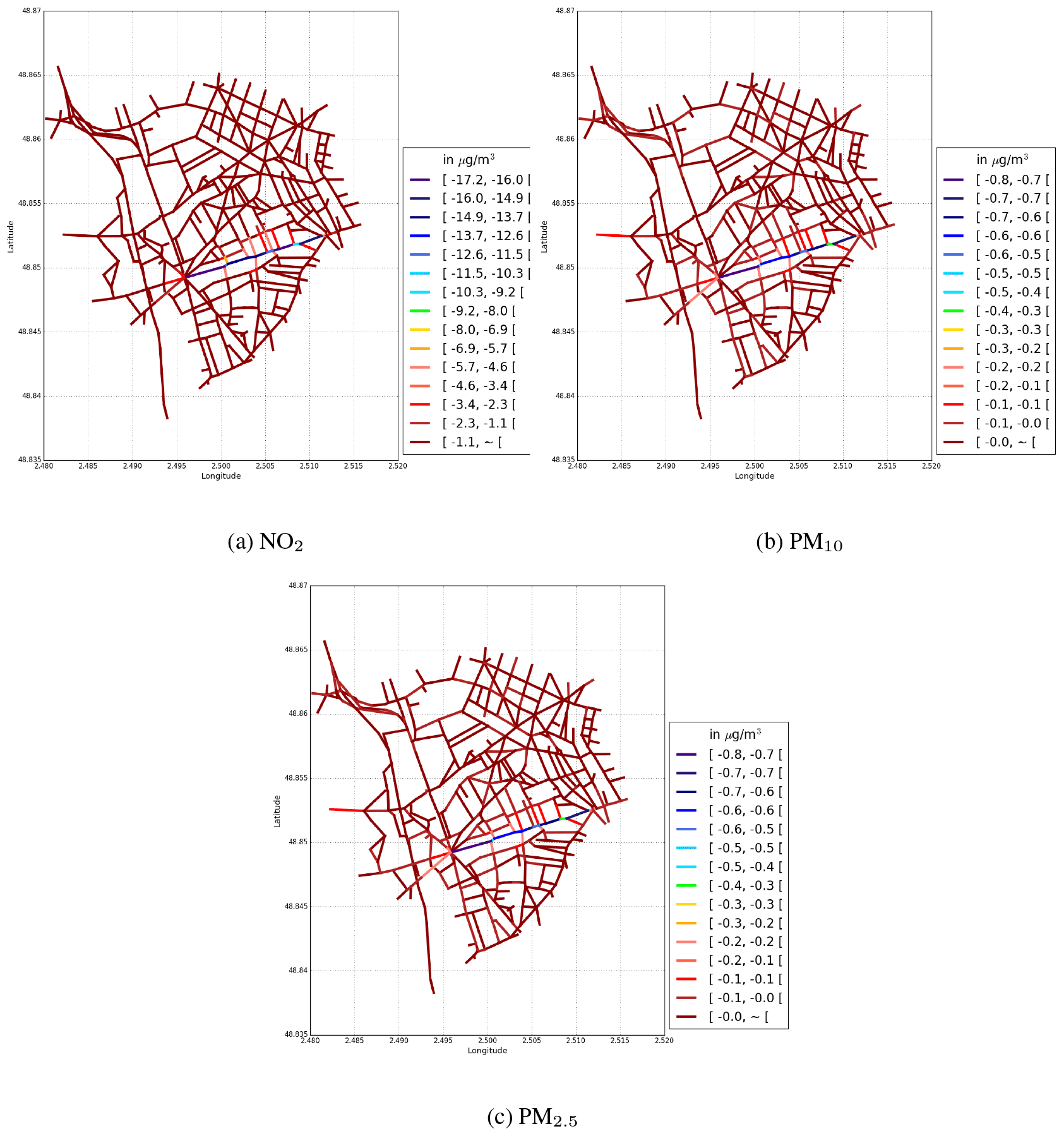
Figure C4 Differences in time-averaged concentrations (in µg m⁻³) between Case-12 and Case-1 (Case-12 − Case-1) for (a) NO₂, (b) PM₁₀, and (c) PM_2.5.