Coupling a large-scale hydrological model (CWatM v1.1) with a high-resolution groundwater flow model (MODFLOW 6) to assess the impact of irrigation at regional scale

In the context of changing climate and increasing water demand, large-scale hydrological models are helpful for understanding and projecting future water resources across scales. Groundwater is a critical freshwater resource and strongly controls river flow throughout the year. It is also essential for ecosystems and contributes to evapotranspiration, resulting in climate feedback. However, groundwater systems worldwide are quite diverse, including thick multilayer aquifers and thin heterogeneous aquifers. Recently, efforts have been made to improve the representation of groundwater systems in large-scale hydrological models. The evaluation of the accuracy of these model outputs is challenging because (1) they are applied at much coarser resolutions than hillslope scale, (2) they simplify geological structures generally known at local scale, and (3) they do not adequately include local water management practices (mainly groundwater pumping). Here, we apply a large-scale hydrological model (CWatM), coupled with the groundwater flow model MODFLOW, in two different climatic, geological, and socioeconomic regions: the Seewinkel area (Austria) and the Bhima basin (India). The coupled model enables simulation of the impact of the water table on groundwater–soil and groundwater–river exchanges, groundwater recharge through leaking canals, and groundwater pumping. This regional-scale analysis enables assessment of the model's ability to simulate water tables at fine spatial resolutions (1 km for CWatM, 100–250 m for MODFLOW) and when groundwater pumping is well estimated. Evaluating large-scale models remains challenging, but the results show that the reproduction of (1) average water table fluctuations and (2) water table depths without bias can be a benchmark objective of such models. We found that grid resolution is the main factor that affects water table depth bias because it smooths river incision, while pumping affects time fluctuations. Finally, we use the model to assess the impact of groundwater-based irrigation pumping on evapotranspiration, groundwater recharge, and water table observations from boreholes.

1 Introduction

Regional- and large-scale hydrological models are often used to assess water resource trajectories under different scenarios for climate change, socioeconomic development, and water management. Despite extensive work, at least three challenges persist: appropriately representing groundwater dynamics and flow (Gleeson et al., 2021; Kollet and Maxwell, 2008; Reinecke et al., 2020; Sutanudjaja et al., 2011; Vergnes et al., 2014), including human impact (Hanasaki et al., 2018; Wada et al., 2017, 2014), and improving spatial resolution (Bierkens, 2015; Fan et al., 2019; Wood et al., 2011). The last point can be replaced in part by “representing water flows driven by small-scale topography” and is of interest for processes at large scale and locally relevant applications. Several large-scale hydrological models include representations of groundwater flow between grid cells and interactions among groundwater, soils, and surface water bodies, such as CWatM (Burek et al., 2020), LISFLOOD (Trichakis et al., 2017), ORCHIDEE (Verbeke et al., 2019), ParFlow-CLM (Keune et al., 2016; Maxwell et al., 2015), PCR-GLOBWB (de Graaf et al., 2017; Sutanudjaja et al., 2018), ISBA-CTRIP (Decharme et al., 2019), VIC (Scheidegger et al., 2021), LEAFHYDRO (Martínez-de la Torre and Miguez-Macho, 2019), and WaterGAP (Reinecke et al., 2019a). These models differ somewhat in their implementation, including the physical representation and parametrization of the groundwater. Currently, developments are oriented towards hyper-resolution models (less than or around a 1 km grid) and representing water management (Hanasaki et al., 2022). However, large-scale model resolutions (∼ 10–50 km) remain much coarser than the hillslope-scale controlling hydrologic processes, as hypothesized by Fan et al. (2019) and Swenson et al. (2019). In addition, coarse resolutions of groundwater representation tend to smooth hydraulic gradients, leading to unrealistic aquifer properties (Shrestha et al., 2018), and potentially to underestimate water table depth drawdowns due to groundwater pumping because withdrawals are applied to entire grid cells instead of applied to punctual boreholes.

A proper representation of groundwater is essential to consider lateral groundwater exchanges between grid cells; otherwise, they remain connected only through the river or drainage network. Darcy's law links hydraulic head gradient, hydraulic conductivity, and aquifer thickness and can describe this lateral groundwater flow. Some studies have already highlighted the contribution of lateral groundwater flow to regions and basins (Krakauer et al., 2014; Schaller and Fan, 2009). Groundwater flows redistribute water from hillslope to regional scale, leading to evapotranspiration variability between upstream and downstream areas (Condon et al., 2020; Condon and Maxwell, 2019; Famiglietti and Wood, 1994; Fan and Miguez-Macho, 2010; Keune et al., 2016; Miguez-Macho and Fan, 2012; Swenson et al., 2019). These studies highlight the fact that evapotranspiration is impacted to a greater degree during dry seasons and where the water table is shallow. Oversimplifying lateral water redistribution and exchanges between soils and groundwater may also induce non-negligible evapotranspiration biases (Koirala et al., 2019; Martínez-de la Torre and Miguez-Macho, 2019; Rouholahnejad Freund and Kirchner, 2017; Wang et al., 2018). The impact of the depth of the groundwater level on evapotranspiration and consequently on net groundwater recharge (recharge minus capillary flux) has also been demonstrated by Szilagyi et al. (2013) based on observed depth to groundwater and evapotranspiration estimated from MODIS data and by Koirala et al. (2017) based on simulated depth to groundwater and remote sensing data. Finally, reproducing soil moisture drainage, capillary rise, and baseflow more accurately depends on properly representing groundwater depth and time fluctuation.

Recent studies based on different models (de Graaf et al., 2017; Fan et al., 2013; Martínez-de la Torre and Miguez-Macho, 2019; Maxwell et al., 2015; Sutanudjaja et al., 2014, 2011; Vergnes et al., 2020) have compared simulated and observed water tables at continental and regional scales; these studies have argued that the main spatial trends were well reproduced. However, some of these studies have acknowledged that water table depth is not well reproduced, given the coarse spatial resolution (including problems of the spatial representativity of the boreholes and potential bias sampling) and the lack of representation of water management within the models (Fan et al., 2013; Maxwell et al., 2015; Reinecke et al., 2020). This raises the question of the reliability of such models in terms of parametrization and application (Gleeson et al., 2021). For example, regional- and continental-scale models often assume very simple groundwater pumping schemes or no pumping at all, and they consider these withdrawals to simply leave the system (Vergnes et al., 2020; Surinaidu et al., 2013; Martínez-de la Torre and Miguez-Macho, 2019). Hanasaki et al. (2022) demonstrated the difficulty of introducing regional water management schemes into large-scale hydrological models. Therefore, the interaction between human water management and water availability is a critical aspect of large-scale hydrological models. Humans strongly impact natural water fluxes, affecting available water resources (Keune et al., 2018; Taylor et al., 2012). Irrigation sustained by groundwater significantly impacts the water cycle in several regions (Cao et al., 2016; Dalin et al., 2017; Gleeson et al., 2012; Keune et al., 2018; Siebert et al., 2010; Taylor et al., 2012). To predict future water resources, it is necessary to decipher climate and human contributions contained within the space and time variability of hydrological signals. Large-scale hydrological models have been developed to estimate water availability and water use from surface water bodies and groundwater at a global scale (Döll et al., 2014; Wada et al., 2014). Recently, Hanasaki et al. (2018) improved the representation of human interventions in the H08 model and showed more realistic river discharges and terrestrial water storage anomalies for several huge basins. Sadki et al. (2022) explored the possibility of improving dam representation in the ISBA-CTRIP model applied over Spain. Long et al. (2020) studied the impact of the south-to-north water diversion in China on groundwater pumping using CWatM. Using a global-scale hydrological model coupled with MODFLOW, de Graaf et al. (2019) reproduced the water table drawdown dynamic caused by pumping and its impact on rivers. They determined that rivers reach their environmental flow limit (meaning that groundwater baseflow supporting rivers fails below its 10th percentile as suggested by Gleeson and Richter, 2018) before substantial groundwater depletion occurs.

Studying and simulating regions with significant use of ground and surface waters requires accounting for the management and linkages between the two sources of water. Surface water management and groundwater management are fundamentally connected. Water demand that is satisfied with surface water stored in reservoirs and delivered through pipes or canals may be supplemented with groundwater when the timing or volume of delivery does not coincide with the need. Distribution networks, including urban pipes and agricultural canals, may encourage groundwater recharge through aging and leaking infrastructure. Further, it is necessary to understand who has access to surface water to know where groundwater is the only source that can satisfy the demand. Some farmers will withdraw river water in the rainy season and otherwise depend exclusively on groundwater or leave fields fallow in the dry season. In addition, to understand groundwater's spatial and temporal use it is necessary to appreciate the spatial and temporal distribution of crop water needs.

In this paper, we present refinements on both fronts relative to previous studies by applying the model at finer resolutions,accounting for water management, and comparing simulations with observed water table fluctuations and water table depths. Our new water management representation includes estimating irrigation demand and automatic supply from canals (with potential leakage recharging groundwater), reservoirs, and/or groundwater (Smilovic et al., 2019). To this end, we coupled a high-resolution version of CWatM (∼ 1 km resolution) with MODFLOW implemented at high resolutions of 100 and 250 m. These model versions are used in the Seewinkel region (Austria) and the Bhima basin (India), extending over 573 and 46 000 km², respectively. Studying groundwater processes at regional scale allows for better calibration and validation of models at a high resolution based on observed groundwater levels and estimated groundwater pumping. The Seewinkel area is much smaller and less complex than the Bhima basin regarding the aquifer and less anthropic regarding water management. Comparing the two regions is of interest to evaluate how geological (as well as geomorphological) complexity constrains the model's ability to reproduce water tables. The comparison should also help clarify the impact of two levels of water management on the water cycle.

The remainder of this paper is organized as follows. We first describe CWatM (Sect. 2.1 and 2.2). Section 3 describes the two study regions. Model performance (Sect. 4) is evaluated based on the water table observed in the monitoring well networks. Then we describe the experiment to assess the impact of groundwater-based irrigation on water tables and the water cycle (Sect. 5). The results show the model's ability to reproduce temporal and spatial variability of water table depth (Sect. 6.1). Then the experiment shows how different water cycle components are impacted by irrigation (Sect. 6.2 and 6.3). Finally, we discuss the most critical factors affecting the model's accuracy (Sect. 7).

2 Method

2.1 CWatM

CWatM (Community Water Model) is a distributed hydrological model that can be implemented at regional to global scales (Burek et al., 2020). The model is developed with the Python programming language and is open-access (https://cwatm.iiasa.ac.at/, last access: 13 June 2022). CWatM aims to reproduce the main hydrological processes, including water management. In this study, CWatM is applied in two regions and coupled with a finer-resolution groundwater flow model, MODFLOW (Harbaugh, 2005). CWatM is used at a spatial resolution of 1 km in Seewinkel and ∼ 0.9 km (30 arcsec) in Bhima. Because the Bhima basin covers a large area, CWatM is applied in a geographic projection system (WGS84), while square cells are used for Seewinkel (Lambert azimuthal equal area projection system ETRS89). MODFLOW is applied at 100 m in Seewinkel and 250 m in Bhima using square cells in both regions.

The following sections more extensively describe how groundwater processes and pumping are modeled. The coupled CWatM–MODFLOW uses a computationally efficient approach combining MODFLOW 6's Basic Model Interface (BMI) (Hughes et al., 2017) and Python packages Flopy (Bakker et al., 2016) and xmipy (Russcher et al., 2020). The coupling of CWatM and groundwater is illustrated in Fig. 1. In particular, it is necessary to use high-resolution groundwater models, as topography controls the variability in the water table. For example, Fig. 1 contains an illustration of 1 CWatM cell containing 100 MODFLOW cells (10 shown within the cross-section), and it highlights the fact that different land cover types are considered in each CWatM cell. Soil processes that occur within each land cover part are modeled independently before being averaged according to their respective coverage area within the CWatM cell. This approach allows consideration of the subgrid variability without reducing resolution.

Figure 1 CWatM vertical and lateral sections focusing on coupling with MODFLOW. The CWatM cells are composed of five land cover types: grasslands, grasslands experiencing groundwater (GW) capillary rise, irrigated crops, urban areas, and surface water bodies. The figure illustrates the impact of aquifer pumping on the water table depth and consequently on baseflow and groundwater capillary rise toward soils.

2.2 Including groundwater within CWatM

2.2.1 Representation of soil and groundwater flows

CWatM–MODFLOW simulates subdaily hydrological processes that occur in soil and surface water bodies. Soils are represented in three layers. Unsaturated soil moisture redistribution and capillary rise effects are calculated using the van Genuchten–Mualem equations and soil hydraulic properties (Wösten and van Genuchten, 1988). At every daily time step and within each CWatM cell, the upper soil layer receives infiltration from precipitation and irrigation. If the underlying simulated water table is below the bottom soil layer, water percolates from the deepest soil layer as a function of saturation. This water reaches the groundwater layer of the model as groundwater recharge. If the water table is above the lower bound of the soil, downward percolation does not occur, and groundwater feeds the soil (i.e., capillary flux). Finally, evapotranspiration depletes soil moisture, given the potential evapotranspiration demand and soil water availability.

The groundwater model is implemented using MODFLOW 6. Each day, the coupling is performed based on the following steps (Fig. 2): (1) CWatM initializes the time step and begins processing the surface hydrological components, (2) CWatM simulates the groundwater recharge and extraction, which are converted in memory to MODFLOW inputs, (3) MODFLOW inputs are passed to the MODFLOW model using the BMI, (4) MODFLOW runs the time step using CWatM outputs, (5) MODFLOW outputs (baseflow and groundwater capillary rise) are read into CWatM using the BMI and are converted in memory into CWatM inputs, and (6) CWatM simulates other surface hydrological components. The MODFLOW model can be used at different space and time resolutions.

Figure 2 Scheme of the CWatM–MODFLOW coupling. Conversion refers to changing spatial resolution and units as well as passing to the MODFLOW model using BMI (blue case) or reading MODFLOW output (red case). Note that the MODFLOW model can be used at different space and time resolutions.

CWatM provides a recharge rate to each MODFLOW cell for each time step. However, when the previous simulated water table reaches the top of the aquifer (equal to the bottom of the soil layer), the aquifer cell is saturated. In this case, the recharge rate is set to zero. Recharge occurs once the water table drops below the top of the aquifer. Hydraulic heads, also referred to as a water table here, are computed in MODFLOW by numerically solving the groundwater flow equation (combining Darcy's law and the equation of continuity), considering no anisotropy and with one unconfined layer on the Dupuit–Forchheimer assumption (Eq. 1):

$$\begin{array}{}\text{(1)}& {\displaystyle \frac{\partial }{\partial x}}\left(T{\displaystyle \frac{\partial h}{\partial x}}\right)+{\displaystyle \frac{\partial }{\partial y}}\left(T{\displaystyle \frac{\partial h}{\partial y}}\right)=\mathit{\theta }{\displaystyle \frac{\partial h}{\partial t}}-R\left(t\right)+Q\left(t\right),\end{array}$$

where T is the transmissivity [$L^{\mathrm{2}}/T$​​​​​​​] equal to the hydraulic conductivity (K) times the saturated thickness of the aquifer (e_sat), θ is the porosity, R is the recharge rate [$L/T$], and Q is the pumping rate [$L/T$]. Hydraulic head lateral propagation is controlled by diffusivity ​​​​​​​$D=K\cdot e_{\mathrm{sat}}/\mathit{\theta }$. Upward flow is computed using the DRAIN MODFLOW package when the simulated water table reaches the top of the aquifer. This flow is equal to the difference between the hydraulic head in the cell and the top of the aquifer multiplied by a conductance parameter [$L^{\mathrm{2}}/T$]. This upward flow is partitioned between the baseflow feeding the river's network directly and the groundwater capillary rise feeding the soils. This ratio depends on the percentage of rivers attributed to each MODFLOW cell. Suppose a MODFLOW cell is highly saturated and no river is identified above this cell. In that case, groundwater can indirectly feed the river network through capillary rise. In this area, the soil in CWatM becomes oversaturated, reproducing an area of groundwater overflow.

Moreover, exchanges between groundwater and surface water bodies (lakes, rivers, and channels) are implemented within CWatM–MODFLOW. Below the surface water bodies, if the simulated water table reaches the top of the aquifer (equal to the bottom of the surface water body), an upward flow is sent from the aquifer toward the surface water body. On the contrary, leakage toward the aquifer occurs if the simulated water table drops below the top of the aquifer. Lakes and reservoirs are identified inside the CWatM grid using an identifier and the fraction of the “water” land cover type (as illustrated by the “surface water bodies” fraction receiving baseflow in Fig. 1).

2.2.2 Groundwater pumping

CWatM–MODFLOW simulates water management and demand. Irrigation depends on the fraction of the irrigated crop land cover type on each CWatM cell. Irrigation need is estimated as a function of potential crop evapotranspiration and available soil moisture within the land cover type (Burek et al., 2020). Next, CWatM imposes pumping to the groundwater model for each day. The water demand from all sectors (irrigation, livestock, industry, and households) can be attributed to surface water bodies and to different groundwater model cells depending on where boreholes have been defined in the groundwater model (Fig. 1). Pumping in the aquifer is simulated with the WELL MODFLOW package. Groundwater abstraction can be limited if the water table in the pumping wells drops below a certain depth. This limit can correspond to physical or economic constraints and is adapted to the study areas. Finally, once the water table recovers above this limit, pumping can begin again.

Note that here, we benefit from a new CWatM development, including surface water and agricultural management (discussed further by Smilovic et al., 2019). To appreciate the impacts of surface water management on groundwater, more than 40 reservoirs simulated in the Bhima basin were outfitted with daily reservoir-specific operations and connected to specific spatial distribution areas (command areas) and canal networks. Reservoirs in the model distribute water based on daily command area demand and according to daily maximums with preference given to non-irrigation requests (domestic, industrial, and livestock). A fraction of this water leaks through the canal network. Further, rivers and lakes are set to satisfy some agricultural demands. Water demand may be supplemented with groundwater when surface water volume does not coincide with the need.

For irrigation demand, this study includes more than a dozen spatially distributed crops specific to the given region, each represented by four crop-specific growth stages affecting water use as well as planting and harvest dates. Regions within command areas have access to both surface water and groundwater, while irrigated crops outside command areas only have access to groundwater. Irrigation is applied depending on crop water needs, soil moisture deficits, and surface water and groundwater availability. Several agricultural practices encourage groundwater recharge, such as non-precision irrigation, bare and freshly seeded fields at the beginning of the rainy season (low actual evapotranspiration), and leaky surface water distribution networks.

3 Two study regions with contrasting groundwater dynamics

The two study areas offer the possibility to refine CWatM–MODFLOW spatial resolution and water management, as well as to examine the ability of the model to reproduce groundwater tables for decades, due to the existence of monitoring borehole networks

3.1 Seewinkel region, Austria

The Seewinkel region is a subpart of the Burgenland region in Austria (Karner et al., 2019; Hatvani et al., 2014; Mitter and Schmid, 2021). The study area, of around 573 km², is limited in the west by Lake Neusiedl (Neusiedlersee in German) and in the south and in the east by the border between Austria and Hungary. The Seewinkel region has been classified as semi-arid (Karner et al., 2019; Magyar et al., 2021), even if the aridity index, defined as the ratio between mean annual precipitation and potential evapotranspiration, reaches 1.0. Evapotranspiration shows a strong seasonal pattern, while precipitation is relatively homogeneous throughout the year (Table 1). The region is an important agricultural area, and around 16 % of it is allocated to irrigated crops (maize, potatoes, vineyards, vegetables, and wheat). Only groundwater is used to satisfy irrigation demands. The study area hosts several natural ponds of environmental interest. These ponds mainly depend on the water table in the aquifer. To keep the ponds safe, pumping from irrigation wells is limited when the water table reaches a threshold depth (Magyar et al., 2021). The Seewinkel region and associated groundwater are modestly impacted by human water management.

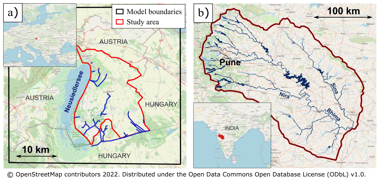
Figure 3 Location of the two study regions. (a) The Seewinkel region in Austria. Blue lines represent canals included in the model. CWatM and MODFLOW are respectively set up at 1 km and 100 m resolutions. (b) The upper Bhima basin in India. Blue lines represent the main rivers. CWatM and MODFLOW are set up at ∼ 0.9 km and 250 m resolutions, respectively.

The CWatM–MODFLOW model (shown in black in Fig. 3a) is applied at 1 km resolution, associated with a MODFLOW resolution of 100 m from a 10 m resolution digital elevation model (DEM; Comprehensive digital field model (DGM) of the state of Burgenland, 2019). To capture the influence of regional groundwater flow, the modeled area is larger than the study area (marked in red in Fig. 3a). Therefore, small ponds are included in the study area, but Neusiedlersee is not. Outside the study area, the percentage of river within each MODFLOW cell is defined from a river network computed with the finer 10 m resolution DEM assuming that rivers are created when the drainage area exceeds 1 km². There is no river inside the study area, but there are several canals draining groundwater. Note that the MODFLOW DRAIN boundary condition on these canals is set at 1 m below the altitude inferred from the 100 m DEM. Groundwater leaving the aquifer below canals and lakes directly reaches the surface water network (see the baseflow in Fig. 1). Using field data, the Seewinkel aquifer is modeled as one aquifer layer with a thickness of 20 m. Regional characteristics and model properties are synthesized in Table 1.

One pumping well is set up every 1 km² at the center of each CWatM cell. Irrigation demand and associated pumping rates depend on the deficit between potential evapotranspiration demand and current soil water contents within the CWatM cell (see the Supplement about the influence of irrigation efficiency and spatial density of pumping wells). Finally, the simulated CWatM–MODFLOW pumping rate at the Seewinkel scale for 2015 is 48 % smaller than the abstraction limits imposed for the year 2015 in Seewinkel. Therefore, the model seems to appropriately represent groundwater use.

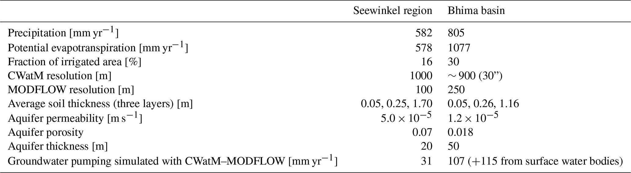
Table 1 Main characteristics and model properties of Seewinkel and Bhima. Annual averages are given for 1983–2016 and 2000–2009 periods for Seewinkel and Bhima, respectively. Aquifer permeability and porosity are obtained after calibration.

3.2 Bhima basin, India

The Bhima basin is located in India and hosts 19 million people. The basin area is 46 000 km². The average aridity index is 0.75 (Table 1); however, precipitation shows strong seasonality due to the monsoon. Both surface water and groundwater satisfy domestic, industrial, and agricultural water demand. Irrigation is by far the most important groundwater use. Around 30 % of the basin area is allocated to irrigated crops. The river discharge recorded at the most downstream gauging stations (Takli) indicates a flow of 120 mm yr⁻¹ on average, but this flows for only 2 months on average.

CWatM is applied at 30 arcsec resolution (∼ 900 m), associated with a MODFLOW resolution of 250 m from a 90 m resolution DEM (Yamazaki et al., 2019). Lakes and reservoirs are marked using HydroLAKES (Messager et al., 2016) and are refined and expanded upon with local data made available by the Pune Irrigation Circle. The percentage of river within each MODFLOW cell is defined from a river network computed with a 90 m resolution DEM, assuming that rivers are created when the draining area exceeds 1 km². In Seewinkel, the aquifer upper limit under the rivers is set at 1 m below the altitude inferred from the 250 m DEM. This correction allows us to better take into account the river incision, which is strongly smoothed when resolution is upscaled to 100 or 250 m. When the water table reaches the top of the aquifer, groundwater is sent either to the soil or to the surface water network (see the groundwater feeding soils and baseflow indicated in Fig. 1) based on the river percentage map. In Bhima, canal networks are added to bring water from reservoirs toward cultivated areas where water is required for irrigation (see Sect. 2.2.3). Leakage is considered to occur below these canals through a water conveyance efficiency of 70 %.

The Bhima basin aquifer was modeled with MODFLOW in Surinaidu et al. (2013) at 1 km resolution, assuming spatially uniform recharge and pumping, deriving each as a linear relationship with precipitation, incorporating different data sources. The ranges for hydraulic conductivity and specific yield used for calibration were also used for this study, and we refer the reader to Surinaidu et al. (2013) for a more detailed description of the region. The model presented here expands on this by including surface water hydrology and management, spatially distributed groundwater recharge and outflow (pumping, capillary rise, and baseflow), and spatially distributed non-irrigation demand, as well as by modeling crop-specific irrigation demand and increasing the spatial resolution. While the Seewinkel alluvial aquifer was identified, the Bhima basin is much larger and is not composed of one homogeneous aquifer alone. The area hosts crystalline rocks, where weathering may potentially enhance permeability and porosity. We considered one homogenous aquifer layer with a thickness of 50 m (Surinaidu et al., 2013). We set up one pumping well in every MODFLOW cell (see the Supplement regarding the influence of irrigation efficiency and the spatial density of pumping wells). As for the Seewinkel model, pumping rates depend on the deficit between potential evapotranspiration demand and soil water content in each CWatM cell. Finally, the imposed pumping rate depends on the fraction of irrigated areas above each pumping well. Pumping is prevented when the water table falls below a depth of 15 m (Surinaidu et al., 2013).

Table 1 provides mean simulated water withdrawals. Annual surface water and groundwater withdrawals within the Bhima basin are estimated for different sectors for 2013 in the upper Bhima subbasin draft report. The model simulates these withdrawals closely (5 % higher), with higher groundwater use and lower surface water use. Through discussions with local water managers and engineers, including through stakeholder workshops (Karutz et al., 2022), it was found that groundwater use is generally underreported and underestimated for both irrigation and non-irrigation purposes. Further, canal leakage is not included in the report, producing an underestimation of groundwater availability. In agreement with the uncertainty of the reported values and following the expert opinions mentioned above, this model appropriately represents the region's annual surface water and groundwater use.

4 Validation of the hydrological models

4.1 Available observed data

Water table data from 81 and 373 monitoring boreholes were gathered for the Seewinkel and Bhima areas, respectively. These observed datasets come from the eHYD (https://ehyd.gv.at/, last access: 3 January 2021​​​​​​​) database in Austria (BMLRT, 2020) and the Central Groundwater Board in India. They have been preprocessed to make them compatible with the simulated water table. First, boreholes close to the model's boundary limits were removed, given that the simplified no-flow boundary condition in the groundwater model could lead to an unrealistic water table in these parts. Second, boreholes were removed where time data covered less than 50 % of the simulation period. Third, we did not consider 5 % of the remaining boreholes with the greatest discrepancy between simulation and observation because they are impacted by specific local conditions that are not well reproduced by the model. This prevents them from influencing the calibration. Indeed, because of model assumptions such as homogeneous aquifers or pumping well locations, it can be inferred that some boreholes could not be well represented by the model due to the vicinity of pumping wells, rivers, or local heterogeneities. Finally, we kept 62 and 351 boreholes for the Seewinkel and Bhima areas (Figs. 4a and 5a), respectively. In the Bhima basin, we also used daily discharge data aggregated at a weekly scale at five gauging stations from the National Hydrology Project in India.

4.2 Comparison between observed and simulated water table

To fully benefit from the informative content of the observed water table, we separately evaluated time-averaged water tables (static part) and water table time fluctuations (transient part). This was done to better understand how each parameter is sensitive to both static and transient parts of observed data. As described above, the calibration relies on 62 and 351 boreholes for Seewinkel and Bhima, respectively.

First, we assessed the model's ability to reproduce the mean spatial variability of the water table driving the lateral groundwater flow. Observed and simulated water tables were averaged along the calibration period at each borehole. However, a comparison between observed and simulated water tables is not relevant and not sensitive to parameters, as the water table mimics the surface elevation, which extends to several orders of magnitude, as noted by Gleeson et al. (2021) and Reinecke et al. (2020). Indeed, the observed water table varies from 430 to 1000 m in Bhima, while observed water table depth varies from 1 to 20 m. Moreover, model topography can differ from actual topography. On the other hand, water table depths contain more discriminant information and are essential for the interaction between groundwater, soil, and surface. Therefore, we compared the water table depth (WTD) instead of the water tables. As a criterion, we used the “normalized mean water table depth difference” [%], defined by the following equation (Eq. 2):

$$\begin{array}{}\text{(2)}& C_{\mathrm{mean}}=\mathrm{100}\times {\displaystyle \frac{\mathrm{1}}{n}}\times \sum _{i=\mathrm{1}}^n\left|{\displaystyle \frac{{\stackrel{\mathrm{‾}}{\mathrm{WTD}}}_{\mathrm{obs},i}-{\stackrel{\mathrm{‾}}{\mathrm{WTD}}}_{\mathrm{sim},i}}{{\stackrel{\mathrm{‾}}{\mathrm{WTD}}}_{\mathrm{obs},i}}}\right|,\end{array}$$

where n is the number of monitoring boreholes, obs and sim refer to observed and simulated depths, respectively, and $\stackrel{\mathrm{‾}}{\mathrm{WTD}}$ refers to the time-averaged WTD. Note that ${\stackrel{\mathrm{‾}}{\mathrm{WTD}}}_{\mathrm{obs},i}$ ranges from 0.25 to 12 m and from 1 to 20 m for Seewinkel and Bhima, respectively. Thus, shallow water table depths do not have too much weight on C_mean.

The second criterion focuses on time fluctuations in water tables observed in boreholes, whatever the mismatch value between observed and simulated time-averaged water table depth. Water table fluctuations correspond to the initial signal after the time average is removed. To simplify, we averaged observed and simulated water table fluctuations from all boreholes instead of comparing the fluctuations at each borehole. This approach smooths local behaviors and informs the water table fluctuations (WTFs) at the basin scale at the first order. As a criterion, we used the normalized root mean square error [%] on average time fluctuations, defined by (Eq. 3):

$$\begin{array}{}\text{(3)}& \mathrm{nRMSE}={\displaystyle \frac{\mathrm{100}}{\mathrm{SD}\left({\mathrm{WTF}}_{\mathrm{obs}}\right)}}\sqrt{{\displaystyle \frac{\mathrm{1}}{n_{\mathrm{obs}}}}\times \sum _{t=\mathrm{1}}^{n_{\mathrm{obs}}}({\mathrm{WTF}}_{\mathrm{obs},t}-{\mathrm{WTF}}_{\mathrm{sim},t}{)}^{\mathrm{2}}},\end{array}$$

where n_obs refers to the number of observations in time (t). Thus, the nRMSE corresponds to the root mean square error (RMSE) expressed as a percentage of the standard deviation (SD) of the observed data.

CWatM–MODFLOW simulation starts in 1981 and ends in 2016 for Seewinkel, while it begins in 1993 and ends in 2009 for Bhima. For both regions, models are run the first time during the whole period to initialize the water table. For Bhima, hydraulic conductivity and specific yield variables were included first in a calibration (Fortin et al., 2012) using five daily discharge stations (2000–2009), and ranges for calibration were derived from Surinaidu et al. (2013). The top 20 % from the discharge calibration was further analyzed for water table fluctuation and depths. Groundwater parameters hydraulic conductivity and porosity are further calibrated by comparing the simulated and observed water table recorded monthly in boreholes from 1983 to 2016 and twice a year from 1997 to 2009, respectively, for Seewinkel and Bhima. Standard CWatM parameters were used in Seewinkel. Therefore, only groundwater parameters are calibrated in this study.

5 Experiments to infer the impact of irrigation

The effects of irrigation are evaluated by comparing simulations with and without irrigation. To infer the effects of irrigation during the simulation period, we focus on the annual average of several variables (Fig. 1): groundwater store, soil water content, evapotranspiration, groundwater recharge, and the fraction of humid areas (areas where groundwater often feeds soils). We focus on the impact of irrigation on actual evapotranspiration rate and groundwater recharge in two land cover types, namely groundwater-supported grasslands and irrigated areas. We expect that irrigation will increase evapotranspiration in irrigation areas and reduce evapotranspiration (and increase recharge) in non-irrigated areas. In Seewinkel, we also assess the impact of irrigation during the very dry summer of 2003, as we expect a more substantial effect of irrigation during that period. We also adjusted the irrigation efficiency parameter, which also impacts groundwater pumping, as well as the spatial density of pumping wells to test the sensitivity of the results to these settings (Supplement).

Land cover variability within the CWatM–MODFLOW grid cell is considered using a subgrid approach. Each CWatM cell includes five land cover fractions: grasslands (including non-irrigated crops), irrigated crops, groundwater-supported grasslands (Fig. 1), urban areas, and water body areas. For each CWatM cell, the sum of each land cover fraction equals 1. Here, groundwater-supported grasslands have the same properties as grasslands but correspond to land fractions where groundwater often feeds soils. Setting up a groundwater-supported grassland fraction allows the groundwater flow to be concentrated toward the fraction of the soil that usually receives groundwater instead of distributing this flow homogeneously over all CWatM grid cells (Fig. 1). By this means, we can better take advantage of the finer resolution of the groundwater layer (100 or 250 m). Consequently, soil moisture, surface runoff, and evapotranspiration are more pronounced in groundwater-supported grasslands than in regular grasslands. Technically, the groundwater-supported grassland fractions need to be estimated after an initialization simulation to infer the groundwater-supported areas. Thus, the calibrated CWatM–MODFLOW model is run for the first time during the simulation period to initialize the water table and to define the groundwater-supported fraction for each CWatM grid cell. From this first simulation, MODFLOW cells are defined as groundwater-supported areas if groundwater feeds the soil for more than 4 months out of 12. Then, groundwater-supported fractions are computed at CWatM resolution and used during simulations. Because this land cover fraction is constant over time, the groundwater-saturated land fraction may exceed some grid cells' predefined fractions during extreme events. In this case, groundwater is also sent to other land cover types (grasslands and irrigated areas). In other cases, when the simulated groundwater-saturated area is smaller than the predefined groundwater-supported area, groundwater is distributed equally within the groundwater-supported fraction. Therefore, choosing a threshold of “4 months out of 12” is a compromise allowing us to focus on areas significantly supported by groundwater. This illustrates the importance of simulating water table depths well.

6 Results

6.1 Groundwater parameters

Optimal aquifer permeability and porosity (Table 1) are compared to different datasets as described below. The permeability and porosity in Seewinkel are 5 × 10⁻⁵ m s⁻¹ and 0.07, respectively. These values are respectively 3.10⁻⁴ m s⁻¹ and 0.19 in the global GLHYMPS database (Gleeson et al., 2014; Huscroft et al., 2018). The imposed aquifer thickness (20 m) agrees with the global depth-to-bedrock map (Shangguan et al., 2016), where the average value for the study area is around 22 m.

In Bhima, the permeability and porosity are 1.2 × 10⁻⁵ m s⁻¹ and 0.018, respectively. These values are respectively 3.16 × 10⁻⁶ m s⁻¹ and 0.09 in the global GLHYMPS database. The global depth-to-bedrock values consider thinner aquifers in this region (from zero to a few meters) compared to the imposed aquifer thickness (50 m). Note that for similar permeability (1 × 10⁻⁵ m s⁻¹) and thickness (50 m), Surinaidu et al. (2013) calibrated a porosity of 0.01–0.03 in a regional model. This suggests that permeability is underestimated and porosity overestimated in GLHYMPS over this basin.

6.2 Validation

The model reproduces the time-averaged water table depths recorded in boreholes in Seewinkel (Fig. 4b), with a C_mean value of 38 %. Therefore, we can infer that the hydraulic gradient and water table depth are reasonably well reproduced. The results for the Bhima basin show more contrast (Fig. 5b), as the C_mean is 69 % and simulated water table depth is too shallow on average. Indeed, the simulated mean water table averaged over all monitoring wells is 1.7 m higher than the observed mean in Bhima (Fig. 6b), while the model shows a slight bias of 0.5 m in Seewinkel (Fig. 6a). The reason for this bias is examined in the Discussion section.

In Seewinkel, the observed mean water table lies above a 1 m (2 m) depth for 17 % (47 %) of monitoring wells, while this fraction is 29 % (56 %) in the model (Fig. 4b). Thus, the model overestimates very shallow conditions (<1 m depth). The total land fraction where the simulated mean water table is shallower than a 1 m (2 m) depth is 25 % (46 %). Thus, it can be inferred that a non-negligible land fraction hosts shallow groundwater in Seewinkel.

In Bhima, the observed mean water table lies above a 1 m (2 m) depth for 0 % (2 %) of monitoring wells, while this fraction is 17 % (32 %) in the model (Fig. 5b). Thus, we conclude that the model overestimates shallow conditions in Bhima. Moreover, the total land fraction where the simulated mean water table is shallower than a 1 m (2 m) depth is 6 % (10 %), indicating that monitoring wells are preferentially located in shallow areas.

Figure 4 (a) Map of the monitoring boreholes in the Seewinkel region. (b) Comparison between observed and simulated time-averaged water table depth. (c) Comparison between monthly observed and simulated water table time fluctuations averaged across all monitoring boreholes and expressed as anomalies (relative to the time average).

Both models successfully reproduce water table fluctuations averaged across all monitoring boreholes (Figs. 4c and 5c). The nRMSE reaches 52 % and 41 % for the Seewinkel and Bhima models, respectively. While the primary seasonal and interannual behavior is well reproduced in both areas, some events or periods are not well captured. For example, the Seewinkel model underestimates simulated fluctuations from 1986 to 1988. In addition, fluctuations are overestimated from 2000 to 2005, but the seasonal amplitude is slightly underestimated. In the Bhima basin, it also appears difficult to reproduce several interannual fluctuations and seasonal behavior at the same time. For example, changing the hydraulic parameters to increase seasonal amplitudes from 2003 to 2005 would decrease the base level even more during this period (Fig. 5c). Likewise, increasing or decreasing pumping rates would improve the mean water table bias but would increase the nRMSE focused on water table fluctuations (Supplement).

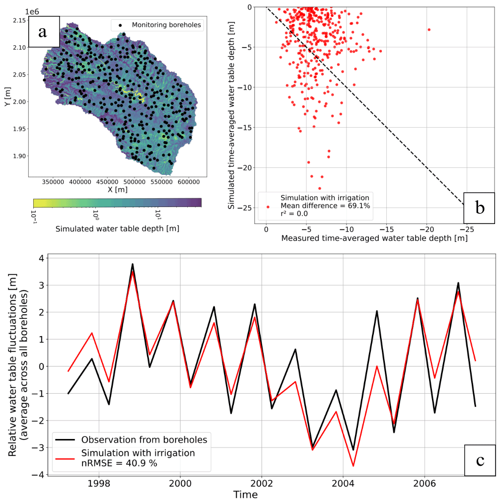
Figure 5 (a) Map of the monitoring boreholes on the Bhima basin. (b) Comparison between observed and simulated time-averaged water table depth. (c) Comparison between observed and simulated water table time fluctuations averaged across all monitoring boreholes and expressed as anomalies (relative to the time average). Based on the daily simulation, the simulated water table is compared on the same days as the observed water table twice a year, before and after the monsoon.

A comparison between observed and simulated weekly discharge in the Bhima basin is provided in the Supplement. The Kling–Gupta efficiency (KGE) (Gupta et al., 2009) values are 0.75, 0.68, 0.54, 0.76, and 0.66 from upstream to downstream stations. These results and the associated good criterion on water table fluctuations (nRMSE) make us confident that the model simulates rainfall partitioning between discharges and evapotranspiration wells.

6.3 Impact of pumping on the water table

The impact of pumping on the water table is a function of mean pumping rate and aquifer properties (permeability, saturated thickness, and porosity). Groundwater pumping theoretically decreases the water table within and around irrigated areas. The results show that groundwater pumping enhances the seasonal water table fluctuations by intensifying water table recession during the dry season in both regions (Fig. 6). It is also shown in Fig. 6 that irrigation accentuates water table depletion during the driest years. Interestingly, during the recharge seasons, the water table within the borehole network is not strongly influenced by pumping in the two study regions, as the water tables with and without pumping are very close (Fig. 6). Because the water table is a proxy for groundwater storage, this result indicates that groundwater storage recovers rapidly and/or irrigation enhances net groundwater inputs. However, this is not the case for the driest periods (i.e., 2004–2005 in Seewinkel and 2003–2005 in Bhima).

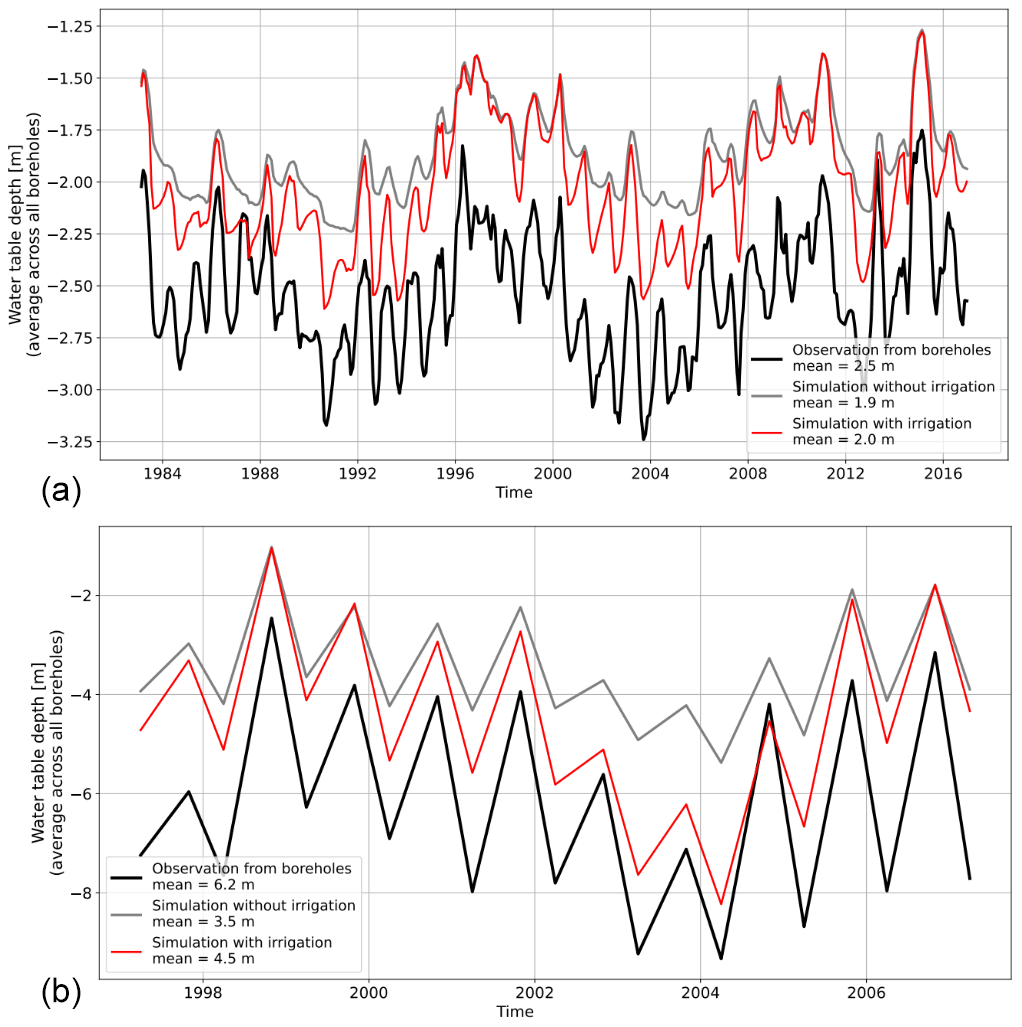
Figure 6 Comparison between absolute water table depth fluctuations obtained from CWatM with (red lines) and without (gray lines) irrigation in the Seewinkel (a) and Bhima (b) areas. Black lines represent observed data. Water table depth fluctuations are aggregated from 62 and 351 boreholes for Seewinkel and Bhima, respectively.

Comparing models with and without irrigation allows us to infer the impact of pumping on the water table. However, groundwater recharge is impacted by irrigation, as we elaborate in the next section. Pumping reduces the average water table at boreholes from 0 during the wet season to around 30 cm and 1–2 m during the growing season in Seewinkel and Bhima, respectively (Fig. 6). The impact of pumping also varies spatially, depending on whether the monitoring borehole is located near the irrigation areas where pumping occurs. Drawdown due to pumping obtained on the time-averaged water table in monitoring boreholes varies between 0 and 50 cm and between zero and a few meters for Seewinkel and Bhima, respectively.

The impact of pumping on the water table is more pronounced in Bhima than in Seewinkel (Fig. 6). This can be explained in two ways. First, aquifer permeability, thickness, and porosity are higher in Seewinkel (5 × 10⁻⁵ m s⁻¹, 20 m, and 0.07, respectively) than in Bhima (1.2 × 10⁻⁵ m s⁻¹, 50 m, and 0.018). Therefore, water table drawdowns around pumping wells are less pronounced in Seewinkel. Second, the mean pumping rate is smaller in Seewinkel (31 mm yr⁻¹) than in Bhima (107 mm yr⁻¹).

6.4 Impact of irrigation

As expected, irrigation increases the total actual evapotranspiration in the two study regions. In Seewinkel, evapotranspiration in irrigated areas increases from 77 to 87 mm yr⁻¹. In Bhima, evapotranspiration in irrigated areas increases significantly from 102 to 209 mm yr⁻¹. However, these changes in evapotranspiration are substantially smaller than the allocated irrigation withdrawals due to conveyance and application losses and the fact that some of the irrigated water reaching the soil percolates toward the groundwater without being used by crops. Indeed, groundwater pumping amounts to an annual average of 31 mm yr⁻¹ in Seewinkel, while annual groundwater and surface water withdrawal amounts to 107 and 115 mm yr⁻¹ in Bhima, respectively. The increase in evapotranspiration is associated with a decrease in river discharge. In Seewinkel, irrigation reduces streamflow from 158 to 152 mm yr⁻¹. However, pumping increases the net lateral groundwater inflow to the study area by around 2 mm yr⁻¹. In Bhima, irrigation reduces streamflow from 257 to 167 mm yr⁻¹. In all, 3 and 14 mm yr⁻¹ from groundwater pumping reach the river network due to irrigation losses in Seewinkel and Bhima, respectively.

Irrigation also significantly increases groundwater recharge in both areas. Recharge increases by 24 % and 50 % in Seewinkel and Bhima, respectively. This is counterbalanced by groundwater pumping such that irrigation causes a reduction of net groundwater input of 12 and 5 mm yr⁻¹ in Seewinkel and Bhima, respectively. However, the net recharge reduction is more pronounced without irrigation from the surface water bodies in Bhima. Indeed, around 40 mm yr⁻¹ of the recharge rise is attributed to irrigation from surface water bodies in Bhima. Note that in both models, irrigation increases recharge in irrigated lands, not only during the irrigation season but also during the wet season (Appendix A1).

Recharge increases not only in irrigated areas (92 % and 94 % for Seewinkel and Bhima, respectively) but also in grasslands (6 % and 5 %) and in groundwater-supported grasslands (2 % and 1 %). These results can be explained by the influence of groundwater pumping, which reduces the water table outside the irrigated areas. When irrigation is not applied, recharge is limited in some periods due to the high water table in groundwater-supported grasslands and episodically in other land cover types. The water table is deeper when irrigation pumping is used, thus enhancing water percolation from the soils to the aquifer. Consequently, soil humidity and evapotranspiration rates decrease in groundwater-supported areas due to irrigation, while recharge increases. This mechanism is illustrated by Fig. 1, which shows a 1D section of a water table with and without irrigation.

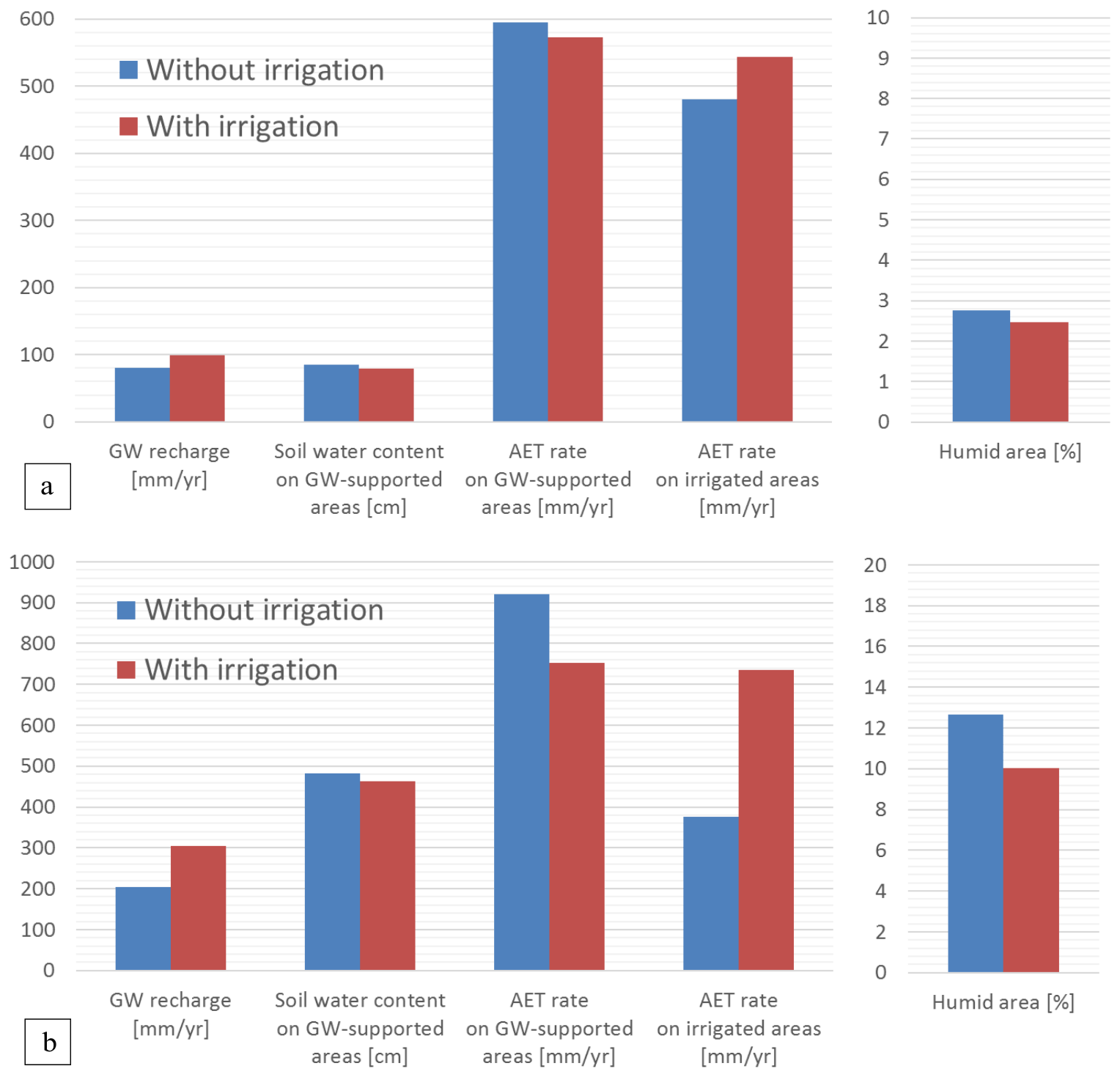
Figure 7 Comparison of some indicators obtained from CWatM–MODFLOW simulation with and without irrigation in annual average values in 1983–2016 for Seewinkel (a) and in 1997–2009 for Bhima (b). Note that the units are different for each variable. Areas were considered humid when the groundwater supported soils for at least 4 months of 12.

In Seewinkel, the mean soil water content in groundwater-supported areas decreases from 85 to 79 cm due to pumping (Fig. 7a). The associated evapotranspiration rate diminishes from 595 to 573 mm yr⁻¹ per unit area of groundwater-supported areas. In Bhima, the mean soil water content in groundwater-supported areas decreases from 48 to 46 cm when pumping is applied, leading to a drop in the associated evapotranspiration rate from 920 to 752 mm yr⁻¹ per unit area of groundwater-supported areas (Fig. 7b).

The water cycle is slightly impacted by irrigation at an annual scale in Seewinkel, and we can expect a more significant impact through the dry season when irrigation withdrawals occur. Focusing on the dry summer of 2003, the soil water content in groundwater-supported areas decreased from 70 to 65 cm due to pumping (Supplement). Consequently, the evapotranspiration rate in groundwater-supported areas decreased from 292 to 274 mm m⁻² and increased by 40 % in irrigated areas.

7 Discussion

7.1 Impact of irrigation on the hydrological cycle

Here, we tested the implication of irrigation using the coupled CWatM–MODFLOW model at very high resolutions and including a fine representation of water management practices. In Seewinkel, groundwater is the only source of irrigation, while surface water in Bhima satisfies half of the irrigation demand. Our experiment to infer the impact of the irrigation highlights the fact that irrigation does not significantly impact the average annual water balance in Seewinkel. However, the impact of irrigation is more pronounced during dry periods (e.g., the dry summer of 2003). The low average pumping rate can explain the small effect of pumping in Seewinkel (31 mm yr⁻¹) compared to the recharge rate (80 mm yr⁻¹). Moreover, the net water balance of the aquifer only drops by 12 mm yr⁻¹ because recharge increases by 19 mm yr⁻¹ due to irrigation. In addition, permeability and porosity in Seewinkel are high enough to limit the water table drawdowns induced by pumping. Finally, the soil storage is larger in Seewinkel than in Bhima (average soil water content in groundwater-supported areas is 85 and 48 cm, respectively), involving less dependence on groundwater (less irrigation and less groundwater recharge).

In Bhima, the experiment reveals that irrigation strongly increases evapotranspiration from irrigated areas and slightly reduces available water in groundwater-supported areas. Consequently, river discharge is strongly diminished. Like Seewinkel, groundwater recharge increases in both irrigated and non-irrigated lands. The inclusion of water transfer within the unsaturated zone, thickened due to pumping, could reduce effective recharge, as pointed out by Cao et al. (2016). However, due to the pumping rate and the thickness of the aquifer, the water table drawdown was much more significant in their study.

Assuming negligible groundwater interaction within irrigated lands, 70 % and 47 % of applied irrigation (without accounting for evaporation and runoff losses) percolates below soils and increases groundwater recharge in Seewinkel and Bhima, respectively. Similar values are identified in several other studies. Estimates of recharge from excess irrigation are variable, range from 0 % to 80 % (Groundwater Resource Committe, 2009; Le Coz et al., 2013; Meixner et al., 2016; Ochoa et al., 2013; Roark and Healy, 1998; Scanlon et al., 2005; Willis and Black, 1996), and depend on the efficiency of irrigation techniques (Grafton et al., 2018; Meredith and Blais, 2019).

In Seewinkel and Bhima, we find that groundwater storage is replenished each year during the wet season in spite of pumping during dry seasons because water tables with and without pumping are very similar during wet seasons (Fig. 6). We infer that this result depends on the studied regions, as explained below. Indeed, the Seewinkel and Bhima aquifers are shallow, and pumping is limited by water table depth thresholds. Consequently, groundwater resources can be replenished during wet seasons. In Seewinkel, pumping is limited to protect the natural ponds sustained by groundwater. In Bhima, pumping is limited due to economic constraints and decreases in aquifer permeability with depth.

Recharge is enhanced where the water table is deep, while soil water content and evapotranspiration increase where it is shallow (Fig. 1) (Martínez-de la Torre and Miguez-Macho, 2019; Swenson et al., 2019). Therefore, the spatial distribution of the water table depth is critical when focusing on the interaction between groundwater and soils. Our results suggest that simulated water tables are overestimated. This point is discussed in the next section. In addition, the model could be improved by allowing crops to draw water directly from groundwater systems where their roots exceed the soil depth and where the water table is shallow. Finally, water table depth representation is also relevant from an irrigation perspective. First, pumping redistributes groundwater, potentially impacting baseflow or neighboring areas. Second, water table depth is a proxy for available groundwater resources. Finally, it affects pumping costs (Turner et al., 2019).

7.2 Difficulty of reproducing water table variability

The primary result of this study is that the coupled CWatM–MODFLOW model managed to reproduce the average water table time fluctuations (Figs. 4c and 5c) very well. This result is in line with other large-scale models (de Graaf et al., 2017; Martínez-de la Torre and Miguez-Macho, 2019; Sutanudjaja et al., 2014, 2011; Vergnes et al., 2020). Groundwater pumping appears to be necessary to reproduce time fluctuation anomalies in the water table (fluctuations are amplified by pumping in Fig. 6). We infer that, by calibrating water table fluctuations separately, we simulated a good combination between groundwater recharge, pumping, and aquifer lateral flow (driven by hydraulic diffusivity). Therefore, water table time fluctuations contain important information (Houben et al., 2022), even when reproducing the absolute water table depth remains challenging, particularly in Bhima, as also noted by Vergnes et al. (2020). Note that here, we initially averaged water table time fluctuations from all boreholes located within the basins, similarly to Long et al. (2020).

By contrast, the spatial distribution of water table depth can be challenging to reproduce and may be less informative because it is subject to spatial resolution and geological heterogeneity. The comparison between observed and simulated water table depth is satisfactory in Seewinkel (Fig. 4b) but only provides first-order satisfaction in Bhima (Fig. 5b). A first explanation for this may be that the Seewinkel aquifer is more homogenous and well known. Consequently, the model can better describe its properties, such as thickness, permeability, and porosity. In contrast, the Bhima basin is much larger and hosts mainly crystalline rocks with potentially variable weathering and fracture density, making its aquifer properties heterogeneous. Beyond the aquifer parameters, the ability to reproduce time-averaged water table depth is constrained by two critical factors in both areas: the pumping rates and the spatial resolution of the groundwater model. These two factors are more acute in Bhima, where pumping is more pronounced and the resolution is coarser (250 m). In both study areas, simulated mean annual pumping rates at the basin scale were validated. However, we acknowledge that pumping estimates could remain uncertain regarding annual averages, seasonal behavior, and pumping well locations.

Groundwater model resolution is critical because degrading resolution smoothens topographical variability. The altitude of local low points in valleys due to river incision, often corresponding to aquifer resurgences, is increased more than it is in neighboring cells when degrading resolution. Consequently, the water table is shallower than expected because the low points locally controlling the water table are higher than expected (see topography and water table comparisons at 100 and 250 m resolution in Appendix A2). This explains why very shallow conditions (<1 m depth) close to rivers are overestimated in Seewinkel despite the 100 m resolution employed. A similar bias was obtained by Maxwell et al. (2015), who used a spatial resolution of 1 km over the continental US.

The weakness of large-scale models for reproducing the spatial distribution of water table depths has been mentioned but not adequately explained in several previous studies (Fan et al., 2013; Maxwell et al., 2015; Reinecke et al., 2020). These studies indicate that mismatch between models and observed data could be due to (i) well representativity within a mesh that is too coarse (see also Martínez-de la Torre and Miguez-Macho, 2019), (ii) well sampling bias, or (iii) groundwater pumping. However, the ability of large-scale models to reproduce water tables remains primordial, and the means of evaluating them should be improved (Gleeson et al., 2021). Here, for the first time, we used a large-scale hydrological model, including groundwater flow and pumping, at a very fine resolution. We note that, as expected, regional models show a better aptitude to reproduce water table depth. For instance, Vergnes et al. (2020) reproduced a mean water table depth on 639 piezometers across several French regions with a median bias of around 3 m. Similarly, Soltani et al. (2021) simulated water tables with an RMSE of 3.8 m based on around 28 000 groundwater head stations in Denmark. Jing et al. (2018) reproduced water table depths with an RMSE of 6.3 m. In this study, we simulated mean water table depths with RMSEs of 1.0 and 5.0 m in Seewinkel and Bhima, respectively. Surinaidu et al. (2013) obtained a similar RMSE in Bhima with a simpler model at a coarser resolution as well as uniform recharge and discharge. However, a comparison with water table fluctuations, depth bias, and surface water flows, including discharge and reservoir levels, was not performed.

We argue that simulated water tables tend to be shallower than the observed water table due to the coarse spatial resolution, as explained above. However, increasing the groundwater model resolution would significantly increase computing time, which makes it challenging to perform sensitivity analysis. Indeed, the same simulation performed in the Bhima basin at a 100 m resolution lasts around 2 d versus 9 h at a 250 m resolution. Figure 8 illustrates how increasing the resolution from 250 to 100 m slightly reduces water table depth bias. While the nRMSE criterion is not significantly better, highlighting the role of heterogeneity rather than spatial resolution, the mean water table depth is now overestimated by 0.5 m instead of 1.7 m (Fig. 8). Reinecke et al. (2019b) focused on the reason for water table depth mismatch and its sensitivity. They highlighted the importance of hydraulic conductivity, recharge, and surface water body elevation. The surface water body elevation can be assimilated to the top of the aquifer in the two CWatM–MODFLOW models described here. Therefore, this critical factor is linked to spatial resolution. By comparison, Reinecke et al. (2019a) improved their RMSE from 54 to 27 m using a resolution of ∼ 9 km and 900 m, respectively. Note that their experiment was located in a steep domain (New Zealand).

Figure 8 Comparison between simulated water table depth using a groundwater model resolution of 250 and 100 m in the Bhima basin. Black lines represent observed data. Water table depth fluctuations are aggregated from 351 boreholes. Note how improving the resolution reduces the water table.

7.3 Importance of implementing a subgrid approach in large-scale models

CWatM uses a mosaic approach to represent the subgrid variability of the land cover type. In addition, we developed a subgrid approach to improve model efficiency, specifically for groundwater exchanges, to benefit from the finer MODFLOW resolution. Indeed, each CWatM grid cell (1 × 1 km) contains a land cover fraction where soil is supported by groundwater. Therefore, we found that the impact of pumping on soil–groundwater exchanges was more significant when groundwater capillary rise focused on a fraction of each grid cell instead of distributing the flow homogenously over the whole cell. This approach enables better simulation of the link between the water table, evapotranspiration, and recharge without refining the CWatM grid.

As pointed out previously, surface water body elevation, linked to the spatial resolution here, is important for simulating absolute water table depth (Reinecke et al., 2019b). This is important, as the river network elevation strongly controls water table depth. Moreover, rivers represent groundwater outlets, as CWatM–MODFLOW generates baseflow based on the simulated water table below rivers. However, a whole cell cannot be entirely assimilated to a river due to the coarse resolution of large-scale models; thus, two critical issues can be noted. First, large-scale modellers never have a map of the actual river network, including the finest low-order and intermittent rivers. They usually generate a river network based on a digital elevation model (Yamazaki et al., 2019), so partitioning between baseflow and groundwater capillary rise is predefined before the simulation. Second, groundwater reaching the top of the aquifer can feed either rivers (as baseflow) or soils (as capillary rise). Our modeling approach relies on a finer digital elevation model used to compute a river network at a resolution finer than the groundwater model (Sects. 2.2.1 and 3). However, we acknowledge that small natural or artificial drains are not included in the model. Then, partitioning between baseflow and capillary rise is defined at the resolution of the groundwater model. This partitioning impacts the depth of the water table. Indeed, increasing the baseflow fraction decreases the water table depth and reduces the soil water availability. Our approach partly deals with this issue as the resolution is very fine (100 and 250 m) and because cells where groundwater oversaturates soils generate overland runoff, feeding rivers.

Other subgrid approaches exist. The TOPMODEL approach (Beven and Kirkby, 1979), for instance, is used in many regional-scale models. It infers subsurface flow convergence based on a finer digital elevation model. Vergnes et al. (2014) also proposed an alternative approach, in which a groundwater flow equation simulates the water table dynamic but capillary rise only occurs in a fraction of the cells based on the distribution of the topography at the subgrid level. Similar approaches are used within CWatM and PCR-GLOBWB when no lateral groundwater flow is considered. Another option is to represent coarse cells or basins with equivalent (representative) hillslopes (Fan et al., 2019; Loritz et al., 2017; Troch et al., 2003). Recently, new hillslope models have been developed for use at a large scale (Hazenberg et al., 2015; Swenson et al., 2019). However, this conceptual modeling approach cannot include regional lateral flow convergences or groundwater pumping. Finally, another approach would be to aim for hyper-resolution in each compartment (surface, soil, and groundwater). However, this would require huge computing capacity to be achievable at a continental scale.

8 Conclusion

Parametrization, spatial resolution, and human water management are significant challenges for implementing physically based large-scale hydrological models. As in Hanasaki et al. (2022), wherein resolution was ∼ 2 km, we applied a large-scale model to two regions, including water management practices with a hyper-resolution of 1 km for CWatM and of 100–250 m for the groundwater model. Benedict et al. (2019) also recently addressed the resolution issue in large-scale models. They found no significant improvement in discharge predictions even after improving the spatial resolution. However, their hydrological model did not include groundwater lateral flow, and resolution was still coarse (∼ 5 km). Reinecke et al. (2020) found that improving resolution alone is not enough to reproduce water table depth distribution. Their finest resolution was ∼ 900 m. After all, we found that improving resolution and model parameters as well as including pumping data are necessary to improve large-scale models. At the same time, calibrating the model at a regional scale with a resolution finer than 100 m appears to be challenging.

Supporting the results of several previous studies, we found that relative water table fluctuations can be sufficiently simulated to infer groundwater model parameters at the aquifer scale (Houben et al., 2022) and to simulate discharge well (Soltani et al., 2021; Sutanudjaja et al., 2014). Calibrating large-scale hydrological models with discharge data and the water table would ensure that the main water cycle is reproduced (evapotranspiration and discharge), in addition to inner processes such as groundwater recharge, baseflow, and groundwater support to vegetation. The evaluation of large-scale hydrological models remains a challenge (Gleeson et al., 2021), as water table depth patterns are difficult to reproduce at large scales. This pattern is only acceptable at the first order in the Bhima basin, even at 100–250 m resolution. This result is explained by the difficulty of including the heterogeneity of groundwater bodies and pumping within the model. After all, improving resolution to 100 m reduced the bias of the depth distribution of the water table. We argue that reproducing mean water table fluctuations and depth distributions without bias constitutes a significant improvement in large-scale hydrological models. Finally, validated models can be used to predict responses to climate and human interventions such as land cover changes and irrigation management.

Appendix A

A1 Impact of irrigation on groundwater recharge

Irrigation increases groundwater recharge in Burgenland and Bhima. Figure A1 shows that irrigation increases recharge during irrigation periods but also during humid seasons when there is no irrigation. During dry seasons, note that recharge is equal or close to 0 mm yr⁻¹ when no irrigation is applied (red lines). During wet seasons, recharge peaks due to rainfall events are amplified because of water applied during the dry season (orange line).

A2 Impact of the spatial resolution on topography and simulated water table

The​​​​​​​ spatial resolution of the groundwater flow model MODFLOW implemented in CWatM–MODFLOW affects absolute water table depths. This is due to the fact that degrading the spatial resolution smooths topography, as highlighted by a 1D section of CWatM–MODFLOW in Bhima (Fig. A2). The resulting simulated water table is affected by the smoothing of the topography, as low points, representing groundwater resurgences, are higher at 250 than at 100 m resolution.

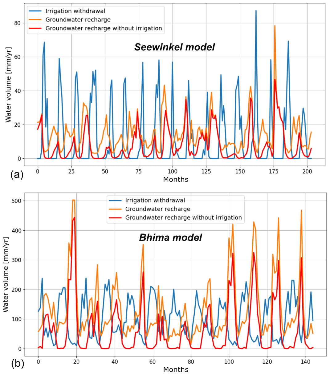
Figure A1 Comparison between average monthly recharge with and without irrigation in irrigated areas in Seewinkel (a) and Bhima (b). Irrigation withdrawal is also represented in blue.

Figure A2 1D section of topography and the simulated water table in Bhima. Comparison between a groundwater model resolution of 100 and 250 m. Note how topography at 100 m resolution is below topography at 250 m resolution in valleys. The resulting water table appears lower at 100 than at 250 m resolution over the whole domain.