the Creative Commons Attribution 4.0 License.
the Creative Commons Attribution 4.0 License.
 | 16 Sep 2022
RavenR v2.1.4: an open-source R package to support flexible hydrologic modelling
James R. Craig
Simon G. M. Lin
Sarah Grass
Leland Scantlebury
Genevieve Brown
Rezgar Arabzadeh
In recent decades, advances in the flexibility and complexity of hydrologic models have enhanced their utility in scientific studies and practice alike. However, the increasing complexity of these tools leads to a number of challenges, including steep learning curves for new users and issues regarding the reproducibility of modelling studies. Here, we present the RavenR package, an R package that leverages the power of scripting to both enhance the usability of the Raven hydrologic modelling framework and provide complementary analyses that are useful for modellers. The RavenR package contains functions that may be useful in each step of the model-building process, particularly for preparing input files and analyzing model outputs. The utility of the RavenR package is demonstrated with the presentation of six use cases for a model of the Liard River basin in Canada. These use cases provide examples of visually reviewing the model configuration, preparing input files for observation and forcing data, simplifying the model discretization, performing realism checks on the model output, and evaluating the performance of the model. All of the use cases are fully reproducible, with additional reproducible examples of RavenR functions included with the package distribution itself. It is anticipated that the RavenR package will continue to evolve with the Raven project and will provide a useful tool to new and experienced users of Raven alike.
- Article
(1754 KB) - Full-text XML
- BibTeX
- EndNote


Hydrologic models are used for numerous applications, including streamflow prediction, flood forecasting, reservoir level forecasting, and in a scientific capacity to advance our understanding of hydrologic systems. Historically, most hydrologic models have been designed with a fixed model structure comprised of a predefined set of environmental processes, whereas the input data and model parameters may vary from watershed to watershed. While these fixed model structures (e.g., GR4J; Perrin et al., 2003) may provide sufficient performance in some catchments, they are not adequate in all catchments, environments, or hydrologic applications (Hoey et al., 2014). Numerous studies have called this fixed structure paradigm into question and have instead called for the development of flexible modelling frameworks (Leavesley et al., 2002; Clark et al., 2011; Fenicia et al., 2011), which would allow the modeller to possess more control over the model-building process. This has resulted in the emergence of flexible modelling frameworks in the literature (e.g., Orellana et al., 2008; Clark et al., 2008; Kavetski and Fenicia, 2011; Clark et al., 2015; Knoben et al., 2019; Coxon et al., 2019; Craig et al., 2020), and recent studies have been extensively supported by the use of these frameworks (Pilz et al., 2020; Remmers et al., 2020; Chadalawada et al., 2020; Knoben et al., 2020; Spieler et al., 2020; Mai et al., 2020; Chlumsky et al., 2021b).
The power contained in these flexible hydrologic models is limited in part by the modeller's ability to take advantage of it. In an ideal setup, a modeller would find converting their system conceptual model to a numerical model a seamless process; in actuality, however, setting up a numerical model often involves data wrangling and other tedious tasks, with decisions ranging from those with relatively little impact on the final modelling results (e.g., how to combine dozens of text files) to potentially problematic and highly impactful decisions (e.g., time series interpolation or model structure adjustments). Few hydrologic models offer the ability to easily deploy and compare successive model runs, resulting in a potentially large amount of time devoted to relatively trivial tasks, such as organizing model files and comparing successive model runs.
In order to address some of these challenges, new tools must be developed to bridge the gap between complex, customizable tools and the ability for modellers (in particular, new users) to fully understand and deploy these tools. Increasingly, freely available, open-source scripting languages, such as Python (Van Rossum and Drake, 2009) and R (R Core Team, 2021), are being employed by modellers to create, visualize, and evaluate their models (Jackson et al., 2019; Slater et al., 2019; Astagneau et al., 2021). The use of these scripting languages also improves the reproducibility of scientific studies, which is a noted challenge in hydrology (Hutton et al., 2016). R, in particular, has gained significant ground in hydrology, entering the toolbox of many in both consulting and academia (Anderson et al., 2018; Slater et al., 2019; Astagneau et al., 2021).
Here, we introduce an R package with a collection of tools to aid a modeller in preparing, running, and post-processing results from custom hydrologic models developed with the hydrologic modelling framework Raven. Many of the tools are not solely Raven-specific: functions exist to plot time series, analyze yearly patterns, and compute relevant statistics. However, the package importantly contains a robust suite of functions for creating, reading, and manipulating Raven model files. Specific attention has been paid to supporting the testing, comparison, and diagnosis of models built with variable model structure; many of these tools are unique. The intended purpose of the RavenR package is to enable modellers to simplify, automate, and document their model creation process; effortlessly facilitate model visualization and evaluation; and to expand the flexibility of the Raven hydrological modelling framework through scripting.
2.1 The Raven hydrologic modelling framework
Raven is an open-source software framework that can be used to build models from a selection of more than 100 available process algorithms (Craig et al., 2020). It is estimated that at least 8×10¹² different hydrologic model configurations may be set up using Raven (Mai et al., 2020), and this number is continuously increasing as new options are added to the software. Raven is built for flexibility, not only in process representation but also in enabling multiple numerical schemes, discretization schemes, input data types, and in providing the user control over output options. Raven is a fully object-oriented code written in C++ (Stroustrup, 2013), and it is typically run from a command line. The input and output files are generally stored as text files (.txt or .csv) or in NetCDF (Network Common Data Format). This allows all model files to be stored as non-proprietary formats as well as to be read and processed with any number of available tools for manipulating files.
The primary input files required for Raven (listed by file extension) include the following:
-
.rvi, which is a primary input file that defines the model structure, time step, duration, and a number of additional options;
-
.rvp, which comprises model parameter specification as well as soil, vegetation, land use, and other class definitions;
-
.rvh, which comprises model discretization, including all subbasin and hydrologic response unit (HRU) information;
-
.rvt, which comprises time series data, including forcing and observational data, and often points to other .rvt files with data sets for various stations and locations;
-
.rvc, which contains the initial conditions for the model run.
Raven provides complete control over its output generation (Craig et al., 2020) – a relatively uncommon feature in hydrologic modelling software. Additionally, it also allows for custom outputs to be generated for a given statistical, spatial and temporal specification and state variable, such as the monthly average of daily snow depth for a particular set of subbasins (Craig et al., 2020). This flexibility of Raven over the modelling process provides the modeller with a lot of power in configuring and running their hydrologic model, but it also provides some challenges with respect to preparing files and working with the many possible outputs. The command-line execution of the program and the lack of a user interface can present a learning curve for new users, but it also enables scripting languages to easily interface with Raven and for Raven to be deployed in high-performance computing environments.
A number of utilities exist to support the usage of Raven models, including RavenPy (https://github.com/CSHS-CWRA/RavenPy, last access: 15 September 2021) for creating, running, and post-processing Raven models within Python, and Hydroglyph (http://raven.uwaterloo.ca/hydroglyph/, last access: 15 September 2021) for visualizing Raven time series output data. Hydrologic model support is also provided by many model-independent packages, such as the CSHS-hydRology package (Anderson et al., 2018). However, RavenR is the most comprehensive tool for preparing input files and performing a range of analyses with Raven output files.
2.2 RavenR software description
2.2.1 RavenR overview
The RavenR package is developed in R and is a collection of tools to aid the modeller in preparing, running, and post-processing files associated with a hydrologic model developed using Raven (Craig et al., 2020). Unlike other software implementations, such as SuperflexPy (Dal Molin et al., 2021), in which the model code is contained within R or Python, the RavenR package is independent of the Raven model code and operates only on related model input/output files and/or calling the compiled Raven executable. This allows for the parallel development of the Raven project and the RavenR library while avoiding the technical challenge of continuously compiling Raven C++ code in R with each build.
The available functions within RavenR can be broadly categorized by their utility into five main categories: (1) preparing input files, (2) running Raven, (3) reading output files, (4) tools for hydrologic analyses, and (5) support utilities (e.g., time series processing and water year analysis). The typical workflow for RavenR is closely related to the workflow required for the development and use of any hydrologic model, including one developed with Raven. This includes the collecting and processing of data for the model, determining the model structure, creating model input files in the format required by the modelling software, executing the model, and analyzing the results of the model for hydrologic consistency and performance. This can include exercises in model calibration and validation, uncertainty analysis, identifiability analysis, and project-specific simulations or adjustments to the model runs.
The typical workflow for developing a hydrologic model and examples of RavenR functions that may be used to support each step are provided in Table 1.
Table 1Typical workflow table for building hydrologic models and connection to RavenR.
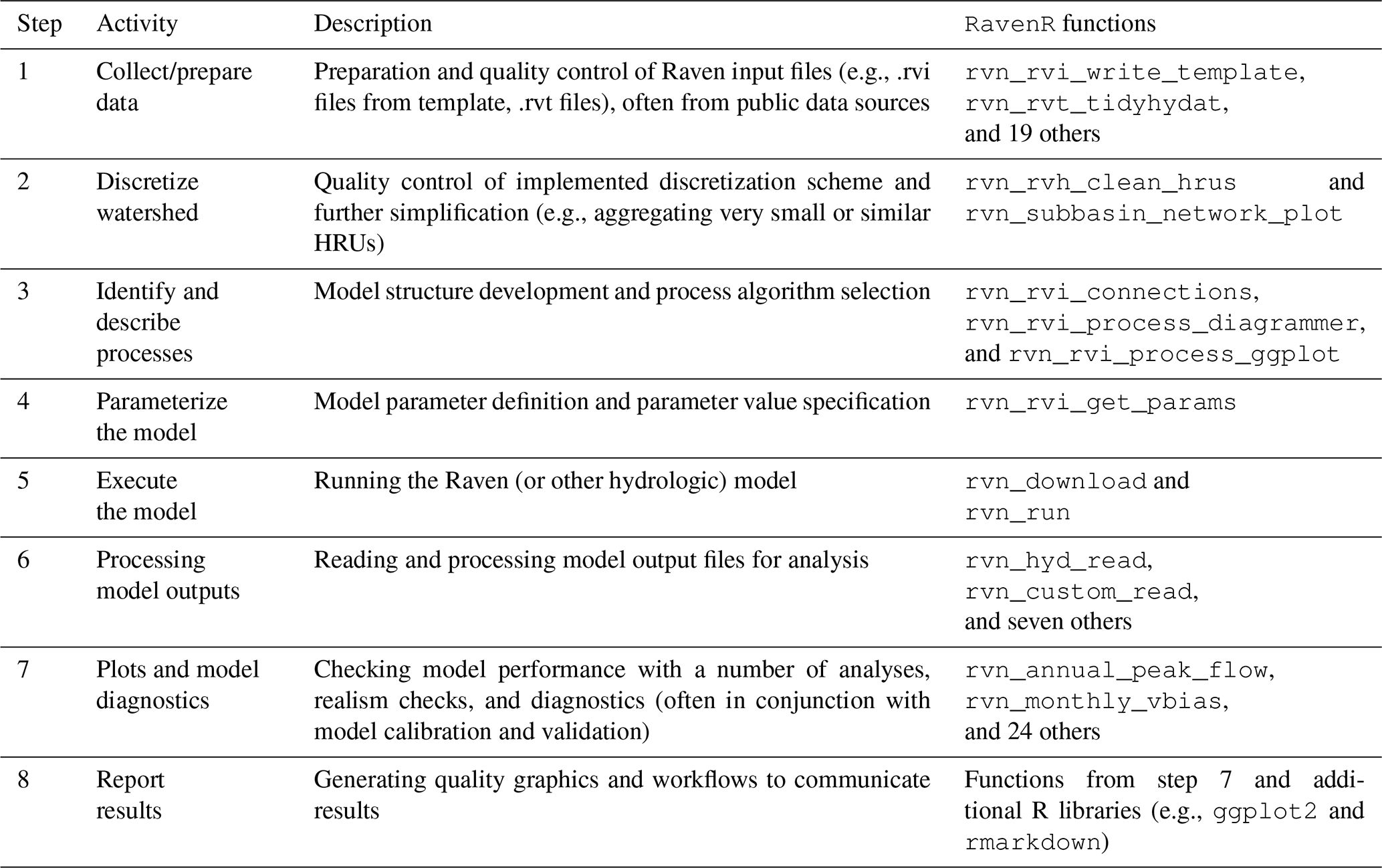
Although the model-building process is listed in Table 1 as a series of steps, it is not linear in practice; rather, it is iterative and cyclic. For example, a model diagnostic (step 7) may show that inadequate model performance can be remedied by the inclusion of additional forcing data, requiring new data to be written to file (step 1). It is also recommended or common practice in modelling to begin with a simpler model and proceed to a more complex one (e.g., Fenicia et al., 2008), which may require iteration on steps 2–6 to potentially modify the structure (e.g., the spatial and temporal discretization and the hydrologic processes) after a basic model has been established. Model calibration would typically involve an iteration upon steps 4–6 with a calibration algorithm, and a calibration that includes model structure (e.g., Spieler et al., 2020; Chlumsky et al., 2021b) would effectively iterate upon steps 3–6. The iterative need for these model-building steps emphasizes the benefit of tools (including those in RavenR) that can reduce the overhead in simple but repetitive tasks, such as producing figures and writing data to a specific file format.
The functions within the RavenR package are named, where appropriate, by the three letter Raven file name or short abbreviation corresponding to the output file that they interact with, e.g., rvn_rvi_connections for processing the .rvi file structure or rvn_res_read for reading the output ReservoirStages.csv file. Other functions simply use illustrative names to convey their purpose (e.g., rvn_budyko_plot). This naming convention provides some navigability of the package functions to the new user, even before the package documentation is reviewed (see Sect. 2.2.2).
The RavenR package has a number of preferred data formats and related package dependencies. Most plots are generated using the ggplot2 (Wickham, 2016) and related libraries from the so-called “tidyverse”, including dplyr (Wickham et al., 2021a) and tidyr (Wickham, 2021) for data manipulation. This allows all plots to be exported as plot objects and further manipulated by the user as desired, and it also removes the need for all plot options to be wrapped into RavenR functions. Time series handling is done through the lubridate (Grolemund and Wickham, 2011) and xts (Ryan and Ulrich, 2020) packages, where the extensible time series (xts) format is generally expected for time series data. Finally, support for network analysis is done through the igraph package (Csardi and Nepusz, 2006), which primarily supports the organization of watershed discretization connections (.rvh file) and the network of model structure connections (.rvi file), including the related plot functions (e.g., rvn_subbasin_network_plot and rvn_rvi_process_diagrammer).
2.2.2 Installation and documentation
The package is developed as a free and open-source software tool, which is ideal for maintaining transparency and reproducibility in workflows related to hydrologic modelling and all steps involved. The stable package version is available for download through CRAN, which can be installed in R using the command install.packages("RavenR"). The development version of the package is available on GitHub (https://github.com/rchlumsk/RavenR, last access: 20 July 2022) and may be installed using the devtools library (Wickham et al., 2021b) as devtools::install_github("rchlumsk/RavenR"). Both installation commands resolve the dependencies associated with the package.
The RavenR package is fully documented and contains a description of inputs and outputs, with a usage example for each function consistent with the standards for CRAN packages. In addition to the package documentation, an introductory vignette Introduction to RavenR, is included with the package, which discusses getting started with the package and how it may be used in a manner that is more useful to new users of Raven and RavenR. The introductory vignette is available with the command install.packages("RavenR").
2.2.3 Sample data sets
In the interest of reproducible examples, the RavenR package contains a number of sample data sets and raw data files embedded within the package which are used within the function examples. Sample data are embedded directly as imported data (accessible with the data function in R) for a number of file output types (e.g., hydrograph and watershed storage) as well as sample data for the tidyhydat and weathercan packages. The latter sample data allow the function examples to run without a dependency on the mentioned data-retrieval packages. Raw data files are also included (accessible with the system.file function in R), which allow for the testing of reading raw data directly. The examples where raw data files are first read into R using RavenR functions may be more helpful than examples which call sample data directly with the data command, as the workflow will be closer to the one applied in practice.
The sample Raven output files and data that are distributed with the RavenR package were generated from a model of the Nith watershed, which is located immediately west of Kitchener–Waterloo in Ontario, Canada. The Raven model of the Nith watershed can be found in full on the Raven web page (http://raven.uwaterloo.ca/downloads.html, last access: 20 July 2022) in the “Tutorial Files # 1–4” download set. Numerous additional Raven models are available from this page, including the model of the Liard River basin (Brown and Craig, 2020), which is used in the RavenR case studies in this paper (Sect. 3).
RavenR package In this section, we present a number of use cases of the RavenR package. These cases are not intended to be a comprehensive review of all the applications for the RavenR package; they serve only to provide the reader with a partial demonstration of how the package may be used in conjunction with Raven. The cases are discussed in the context of hydrologic modelling with flexible frameworks more broadly, and they provide cases and checks that are likely to be useful when deploying both Raven and non-Raven hydrologic models.
The use cases are presented in approximate order of the model-building process (Table 1), beginning with the generation of model input files and proceeding to the analysis of output files. These use cases include examples and discussion of most of the steps in the model-building process, with additional examples available in the use cases markdown file.
All R code and model files required to generate the results and figures in this section are provided in an open-source Zenodo repository (https://doi.org/10.5281/zenodo.5534817; Chlumsky et al., 2022a) and utilize RavenR version 2.1.4 (Chlumsky et. al., 2021a).
3.1 Liard River basin
The use cases presented here utilize the Liard River basin model built with Raven. The Liard River basin is located in northern Canada, spanning the Yukon Territory, Northwest Territories, British Columbia, and Alberta. The Liard River is the largest tributary to the Mackenzie River, with a total contributing area of 275 000 km2 (Brown and Craig, 2020). The basin includes a variety of landforms, including mountainous regions and wetland-dominated regions. There are varying degrees of difficulty when trying to accurately represent these various landforms in a hydrologic model. Additional details on the Liard River basin, as well as the corresponding hydrologic model developed for the basin with Raven, can be found in the publication by Brown and Craig (2020), which also describes the manual calibration process that was undertaken for the model.
3.2 Input file processing
3.2.1 Model configuration
The Raven User's and Developer's Manual (Craig and the Raven Development Team, 2022) provides the templates for a number of model structures, which can be used as a starting point for constructing a customized hydrologic model. These are largely based on emulations of published hydrologic models in the literature (e.g., the University of British Columbia Watershed Model, UBCWM, and the Hydrological Model of École de technologie supérieure, HMETS), although some are based on research models that have been developed within Raven (e.g., the Canadian Shield model). Once a base model has been selected, components of the model may be modified using the many process options available within Raven, which are documented in the Raven User's and Developer's Manual (Craig and the Raven Development Team, 2022). The large number of process options available to the user provide no shortage of model structure tweaks to customize their model.
A critical step in making these adjustments to model structure is understanding the structure and ensuring that it is consistent with the modeller's conceptual understanding of the system (step 3 in Table1). While Raven itself does not currently have a user interface deployed that can visualize the model structure, functions within the RavenR package can generate a model schematic from the contents of the model input (.rvi) file. The ability to visualize this structure can be critical in understanding the model structure and ensuring the conceptual understanding is consistent with the implemented structure. This can also be used to check for state variables or storage units with an improper number of connections, such as a soil layer with no outflow mechanism.
The general workflow within RavenR to generate a model .rvi file and visualize the contents is as follows:
-
A template model structure is selected and written to file using the
rvn_rvi_write_templatefunction. -
The file may be manually modified in consultation with the Raven User's and Developer's Manual (Craig and the Raven Development Team, 2022).
-
The file may be read into R using the
rvn_rvi_readfunction. -
The process connections from the file can be processed using the
rvn_rvi_connectionsfunction. -
The process diagram can be generated either in ggplot format, using the
rvn_rvi_process_ggplotfunction, or as a diagrammer plot, using thervn_rvi_process_diagrammerfunction. -
The “:CreateRVPTemplate” command can be used to generate a template .rvp (parameter) file when Raven is executed. (This step is optional.)
-
The
rvn_rvi_get_paramsfunction may be used to obtain a data frame of parameters, ranges, and default parameter values for parameters that are included in the hydrologic model, based on the model structure configuration. (This step is optional.)
An example of the process diagram is provided for the Liard River basin in Fig. 1. From this figure, the directional connections between water storage compartments in the model can easily be ascertained and verified, allowing both modellers building a new model and modellers inheriting a model to quickly understand the movement of water in their current setup. For instance, in the Liard model, we can see that the model has the capacity for precipitation to enter specific wetland and depression compartments, snow can melt and refreeze, and fast and slow (upper and lower) reservoirs exist to represent groundwater processes at different timescales (Brown and Craig, 2020). A single-layer topsoil compartment is used to connect the surface water and subsurface domains in the model along with a vadose zone reservoir to help represent a karst structure within the model. We can see that all processes that move water to glacier are conditional based on the HRU type (glacier HRU). Ponded water is moved to depression storage under the condition of being a wetland, and surface water only directly evaporates to the atmosphere if the HRU is a lake. The karst groundwater structure which was implemented in the model is only applicable to a subset of the HRUs which accounts for the conditional connections between the top soil layer (SOIL[0]), surface water, the vadose reservoir, and the fast and slow reservoirs. Reviewing and verifying these conditional exceptions along with the connections between other state variables can help ensure that the model is appropriately structured.
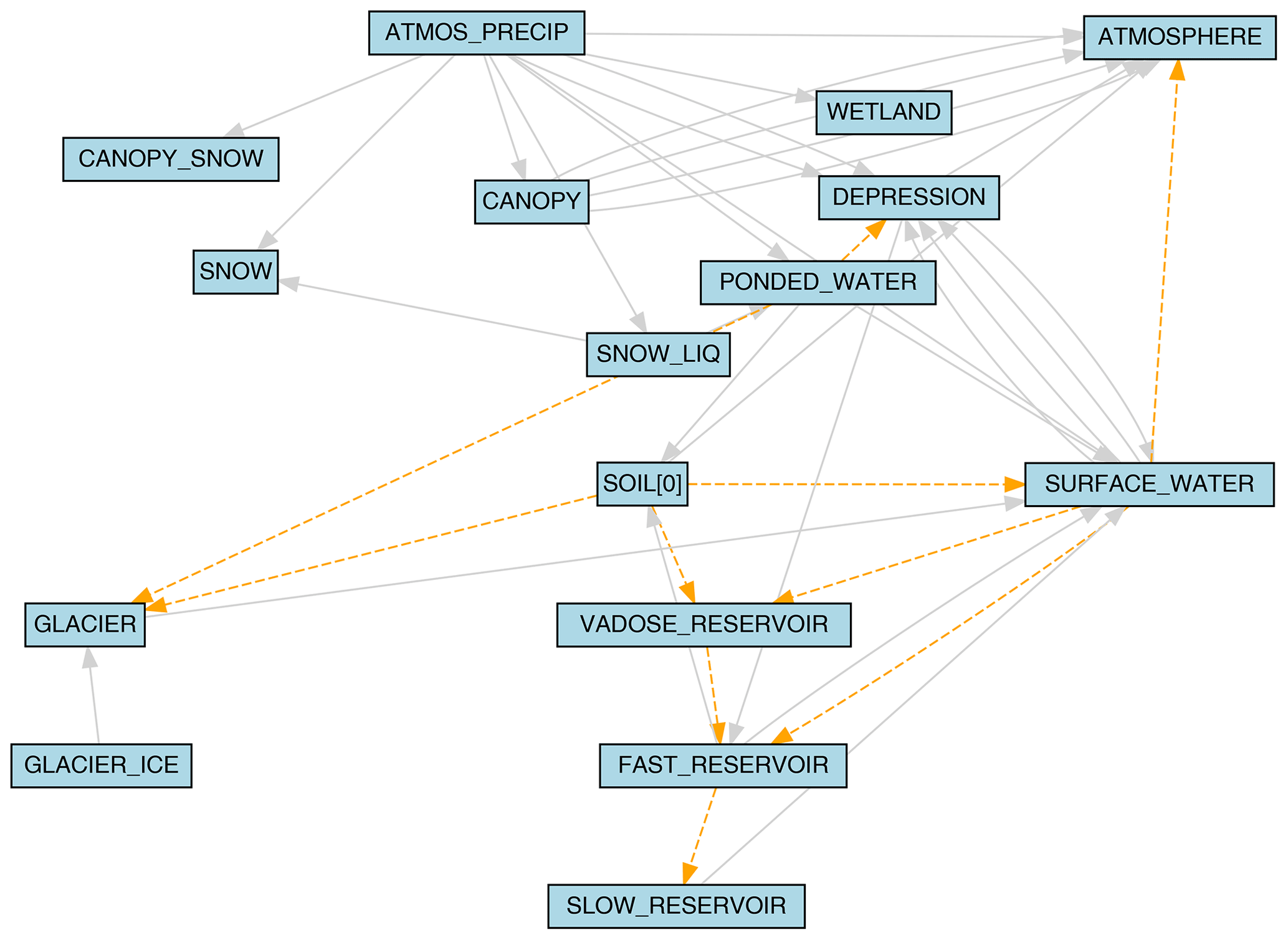
Figure 1The model configuration of the Liard River basin, generated from the Liard model .rvi input file with the rvn_rvi_process_diagrammer function. Solid grey lines indicate connections between state variables, and dashed orange lines indicate conditional connections.
Typically, diagrams such as these are arduous to produce for highly flexible modelling software such as Raven. Here, the function has been automated to create publication-ready diagrams for most model setups.
3.2.2 Forcing data
Meteorological forcings (e.g., precipitation, temperature, and wind speed) drive the hydrologic model responses. When not collected as part of a project, these data are often obtained from online, freely available public sources that are generally collected, processed, and maintained by local and/or public agencies. These data are likely to require some quality control before ingestion into the model, such as addressing data flags, removing erroneous data, and converting units (step 1 in Table 1). This process can be quite tedious, especially when combining multiple data sets with various formats, time steps, and quality levels. The RavenR package offers the rvn_rvt_write_met function for writing forcing data directly to the Raven .rvt format: the function defaults are configured to accept outputs from the weathercan R package, which automatically downloads data for Canadian meteorological stations maintained by Environment Canada (LaZerte and Albers, 2018). For meteorological data sources outside of those obtained with weathercan, substantial data processing may be required to prepare the data into the correct format for use with RavenR.
In this use case, daily meteorological data for a 20-year period are downloaded, interpolated, and written to Raven .rvt format. The weathercan R package is used to search for stations within 500 km of Fort Liard that have data records spanning from 1985 to 2005. A subset of stations meeting these criteria is downloaded for preprocessing. Missing values in the meteorological data are then interpolated using data from nearby stations, and a fix is also applied to any interpolated data where the maximum daily temperature is less than the daily minimum. The data from five of the selected stations are then written to Raven .rvt format. This workflow would require substantial time and effort if performed manually or if scripts for this task were adapted with each new application; in this use case, the entire workflow is performed with two main functions from the weathercan package and two from the RavenR package. The code required to accomplish this is provided in Algorithm 1.
Algorithm 1Minimum code required for the use case described in Sect. 3.2.2 of downloading, interpolating, and writing meteorological data into Raven .rvt format using the weathercan and RavenR R packages. The pipe operator (%>%) from the dplyr package is used for readability. Additional code comments are provided in the accompanying repository.
fort_liard <- c(60.241711, -123.467377)stns <- weathercan::stations_search(coords = fort_liard,dist = 500,interval="day",starts_latest = 1985,ends_earliest = 2006)weather_dl(stns$station_id[1:10],interval="day",start="1985-10-01",end="2005-10-01") %>%rvn_met_interpolate(cc=c("max_temp", "min_temp", "total_precip"),key_stn_ids = stns$station_id[1:5]) %>%
rvn_rvt_write_met()The advantages of this workflow are (1) the ease of implementation, which can process any number of stations with only a few lines of R code, and (2) the transparency and reproducibility of the .rvt file generation, which is useful for both review of the data and possible future corrections to all .rvt files (e.g., extending the time series to incorporate more recent data). The code may be extended to any supplied set of stations and any meteorological variable that is recognized by Raven. The function also assumes standardized Raven parameter units for all meteorological variables (see reference tables in Appendix C of the Raven User's and Developer's Manual; Craig and the Raven Development Team, 2022).
3.2.3 Observation data
Observation data, such as streamflow records, are generally not required to run hydrologic models; an exception to this may be for truncated model domains, where the model simulates a portion of the watershed and is supplemented by upstream measured flow data. However, observed time series are the key to evaluating model performance (history matching) in both calibration and validation exercises and may also be used to enable data assimilation in forecasting applications.
Similar to the use of the weathercan R package for downloading Canadian meteorological data, the tidyhydat R package may be used to download stream gauge data from Canadian stations maintained by the Water Survey of Canada (Albers, 2017). RavenR provides the rvn_rvt_tidyhydat function to process tidyhydat inputs directly by wrapping the rvn_rvt_write function, which can write any non-meteorological time series to .rvt format. Possible types of time series supported by Raven .rvt files include reservoir inflows, irregular observations, observation weights, and temporal reservoir operation rules. The entire list of available formats can be found in the Raven User's and Developer's Manual (Craig and the Raven Development Team, 2022).
In this use case, the tidyhydat package is used to prepare .rvt files of observed streamflow for nine specified stations (consistent with the stations listed in Table 2 of Brown and Craig, 2020) used in the Liard model. The daily streamflow data for these stations are downloaded using tidyhydat from 1985 to the present day, and they are written to .rvt format using the rvn_rvt_tidyhydat function (a wrapper for the rvn_rvt_write function). The code required to accomplish this is provided in Algorithm 2. Raven will automatically exclude any missing values from the calculation of diagnostics; thus, missing values in observation data generally do not need to be interpolated or infilled in the same manner that meteorological forcing data need to be processed. However, the user may still wish to be aware of and avoid large gaps in observation data that may bias the calculation of diagnostic metrics (e.g., consistent winter gaps or multi-year gaps).
Algorithm 2 Minimum code required for the use case described in Sect. 3.2.3 of downloading and writing observed flow data into Raven .rvt format using the tidyhydat and RavenR R packages. The pipe operator (%>%) from the dplyr package is used for readability. Observation station IDs and associated model subbasin IDs are provided in the “observation_stations.csv” file for brevity. Additional code comments are provided in the accompanying repository.
obs_stns <- read.csv("observation_stations.csv")tidyhydat::hy_daily_flows(station_number = obs_stns$stnID,start_date = "1985-01-01") %>%rvn_rvt_tidyhydat(hd, subIDs=obs_stns$subID)The same rvn_rvt_write function may be used to write other .rvt data types by adjusting the rvt_type parameter, which may be useful for writing the observation weights generated from the rvn_gen_obsweights function to exclude certain data periods from Raven diagnostics, as was done in the Liard model for winter periods with unreliable data records (Brown and Craig, 2020).
3.2.4 Model discretization file
The development of distributed and semi-distributed models requires the discretization of a basin into homogeneous units representing hydrologically similar areas. This is typically completed through overlaying a number of spatial data sets which have a dominant effect on the hydrological response of the basin, such as land use, elevation, or soil information (step 2 in Table 1). In overlaying the spatial data sets, a large number of small computational units, insignificant to the model function, can be created. As the model runtime is scaled with the number of HRUs, these small areas can increase computational and calibration runtimes and are not necessary to simulate the dominant hydrological response of the basin. The RavenR package offers a way to effectively eliminate small computational units using the rvn_rvh_cleanhrus function. This function may merge units based on a set area threshold and can also merge similar HRUs based on similarity in HRU properties such as land cover, slope, elevation, and aspect. HRUs that are significant to the model can be locked or protected. Locked HRUs cannot be removed from the model or increase in size, and protected HRUs cannot be removed but may increase in size (to maintain the total watershed area) if other HRUs are removed. This is useful in cases where a point observation is available at a given location (snow survey data) or if the HRUs are part of a significant hydrological response (glaciers).
In this use case, the reduction in the number of model HRUs is demonstrated for a subset of the initial HRUs within subbasin 3 only (initially with 172 HRUs). In the “basic” reduction of HRUs, a simple area threshold is applied. In subsequent examples, HRUs that are of land use type “GLACIER” are locked HRUs (i.e., cannot be removed or change in size), and HRUs that are either “WETLAND” or “WATER” are protected (i.e., cannot be removed but can still increase in size if other HRUs are removed). This operation is applied using area thresholds of 0.5 % (with no locked or protected HRUs), 0.5 %, and 2.0 % of the subbasin area, resulting in 56, 87, and 44 HRUs, respectively. The impact of this operation on land use distribution within the subbasin is summarized in Fig. 2.
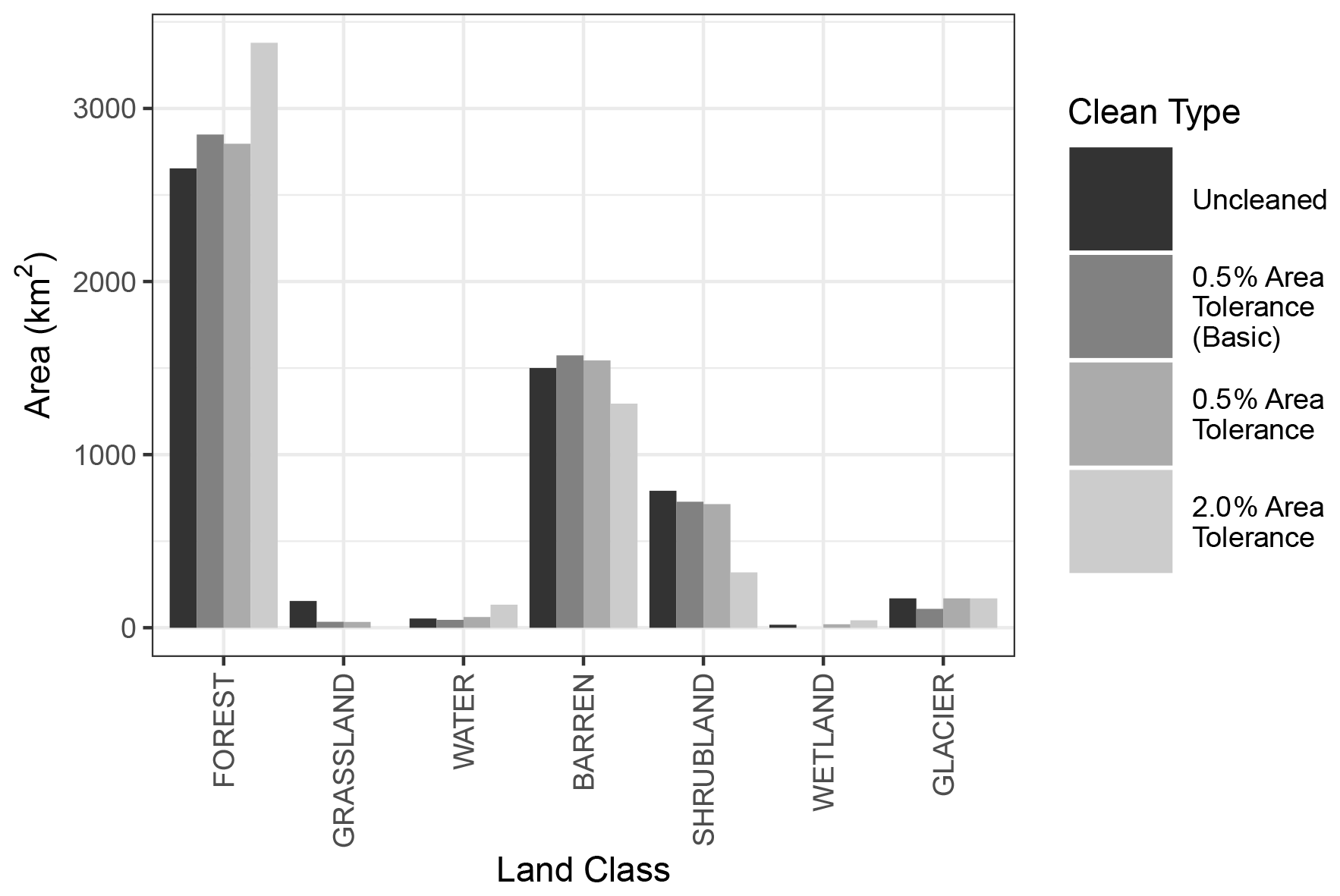
Figure 2A bar plot of total areas by land use for three sets of HRU configurations, including (1) prior to any “cleaning”, (2) following a “basic” 0.5 % area threshold merging criteria with the rvn_rvh_cleanhrus function with no locked or protected HRUs, (3) following the same operation but with locked and protected HRUs specified, and (4) following a 2.0 % area threshold merging criteria. The example is done for a single subbasin in the watershed for demonstration purposes, and it shows how the land use in the subbasin changes when the removal of subbasins below the area percentage threshold is performed, as well as when locked/protected HRUs are introduced, using the rvn_rvh_cleanhrus function.
In the figure, the total area of the GLACIER type decreases in the basic application, but otherwise remains the same when it is locked. The WATER and WETLAND land use types either decrease or reduce to zero in the basic application; otherwise, they increase slightly with each individual cleaning, relative to their proportion of the total area and the total area of removed HRUs based on the respective area threshold. The literature has shown that hydrologic areas such as wetlands that are small in size can still have a disproportionately large effect on the hydrologic and biogeochemical response of the watershed (McLaughlin et al., 2014); thus, retaining particular HRUs or HRU types may be critical in the cleaning of the HRUs. Finally, the plot shows how the other land use types change with these operations. The “FOREST” type increases in each case, suggesting that the proportion of small forested HRUs may be small and that forested HRUs tend to be larger in size. The “SHRUBLAND” HRUs decrease with respect to the represented proportion in each case. This type of analysis could be repeated for other HRU properties (e.g., slope, aspect, and vegetation type). This analysis should be done in conjunction with the use of the rvn_rvh_cleanhrus function to ensure that the reduction in the number of HRUs does not unexpectedly alter the overall representation of HRUs within the model and inhibit the ability of the model to capture the dominant hydrologic response.
3.3 Output file processing and analysis
A number of functions within RavenR are included to handle the reading of common Raven output files, such as the Hydrographs file (rvn_hyd_read), the WatershedStorage file (rvn_watershed_read), and other output files (e.g., forcings and custom output). In addition, functions to analyze the output data with typical hydrologic checks and diagnostics are included in the package. While these functions are built to work with the Raven-specific read functions, they are otherwise not specific to Raven and may be used for any hydrologic model given that a means of reading time series output is provided.
This section provides use cases where the realism of the Liard model is assessed. These checks provide the modeller with an understanding of the model dynamics and provide more confidence that the model is functioning as expected without model compensation errors (step 7 in Table 1). This section also provides a demonstration of tools for evaluating model performance.
3.3.1 Evaluation of model realism
The flexibility of Raven in the generation of model outputs, including customized outputs that may be specified by the user, can be leveraged to undertake rigorous checks of the hydrologic model. Tools have been built into the RavenR package to capitalize on this feature and facilitate a set of model realism checks. Here, we define model realism as the model's ability to replicate and be consistent with anticipated hydrologic behaviour, such as reproducing snowpack measurements and producing reasonable evapotranspiration and runoff coefficients. This definition echoes the one provided in the literature by Euser et al. (2013). These checks can be considered semi-automatic, as a script may be deployed to generate the figures but they still require interpretation by a modeller with an understanding of both the natural system and the developed model. Here, the focus is on the realism of the model to ensure that it is providing hydrologically plausible results; the actual performance of the model with respect to streamflow is discussed further in Sect. 3.3.2.
The checks that are applied to the Liard River basin in this use case include the following: (1) plotting the Budyko curve (Budyko, 1974) for the annual average watershed indices, (2) plotting the annual regime curve with monthly averages, (3) examining the stationarity of moisture content in soil storage layers, and (4) plotting the model performance with respect to snowpack storage as the snow water equivalent (SWE). Additional checks supported (but not demonstrated here) include the following: plotting the forcing functions to understand how the inputs may be influencing the model results (i.e., wet and dry years, erroneous temperature readings, etc.), checking the annual water balance, examining baseflow characteristics by comparing modelled and estimated baseflow from baseflow separation techniques, plotting annual hydrographs in an overlay (i.e., spaghetti plot), and checking the modelled hydrographs and reservoir levels, if any reservoirs or lakes are included in the model.
The four plots associated with the stated checks performed in this example are provided in Fig. 3.
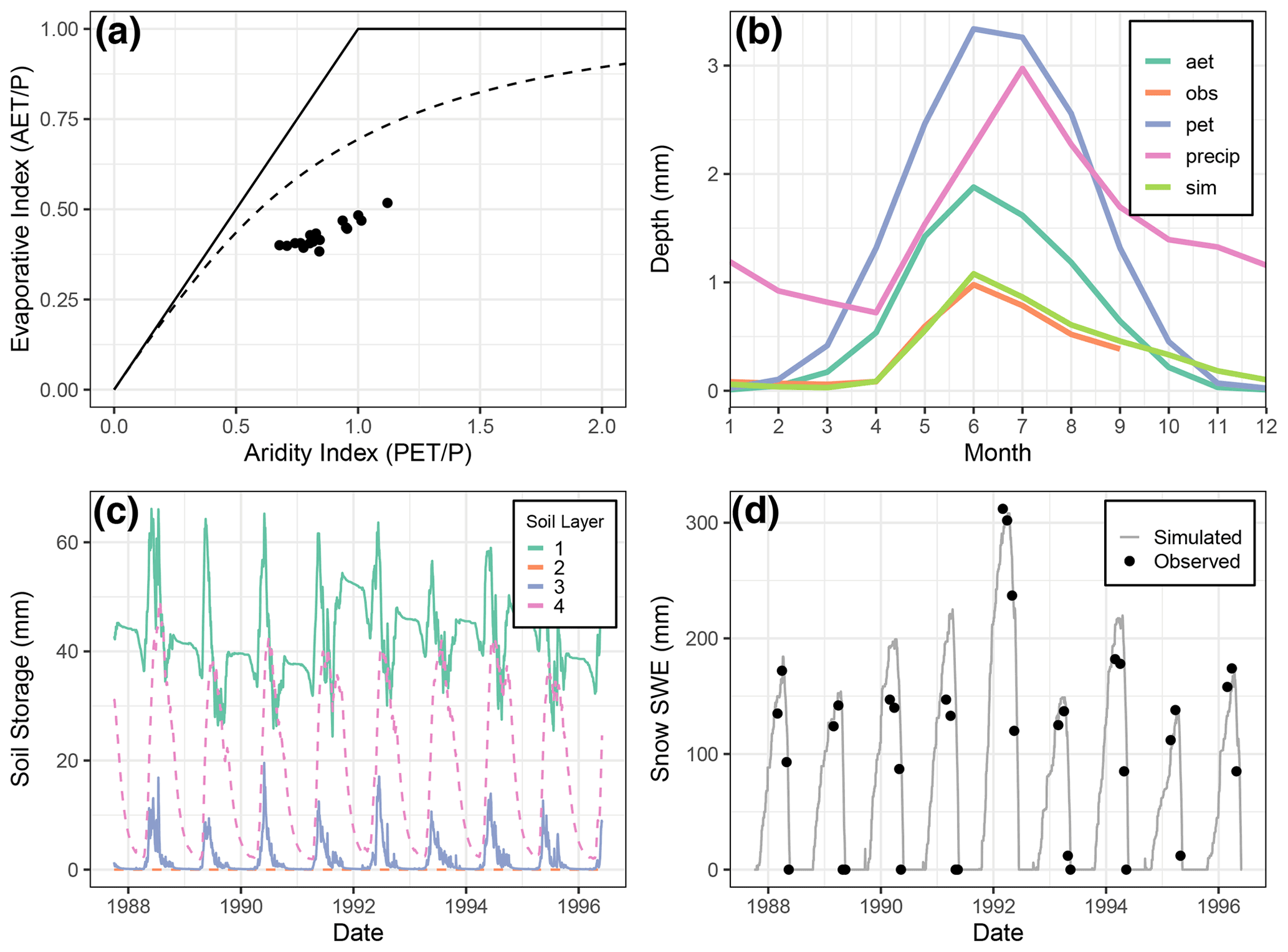
Figure 3Multiple diagnostic plots generated from the RavenR package that may be useful in evaluating the realism of any hydrologic model: (a) Budyko curve with annual average data points for the watershed; (b) a series of regime curves including actual evapotranspiration (aet), observed flow (obs), potential evapotranspiration (pet), precipitation (precip), and simulated flow (sim); (c) soil storage time series showing the stationarity in long-term storage within soil layers; and (d) plots of observed and simulated snowpack measurements at the Frances River. All data are generated from the Raven model averaged at the watershed scale unless otherwise indicated (i.e., snowpack SWE).
The Budyko plot in Fig. 3a was generated using the rvn_budyko_plot function. The Budyko curve (Budyko, 1974) shows the relationship that quantifies how mean annual precipitation is partitioned into discharge or evapotranspiration (ET), where the aridity index is plotted on the x axis, and the evaporative index is plotted on the y axis. The Budyko pattern has been observed in multiple catchments around the world (Vereecken et al., 2015). Certain catchment characteristics, such as significant basin storage or the presence of wetlands (which are present in the Liard model), can cause deviations from the Budyko curve. Deviation from the line may also indicate that actual evapotranspiration is underestimated, which may prompt further examination of the model.
The regime curve can be used to examine the quantities and timing of some of the key model functions. For example, Fig. 3b shows that the potential evapotranspiration (PET) in the Liard model peaks at the same time as the actual evapotranspiration (AET) in June, and the simulated and observed flows (sim and obs variables, respectively) are close in value – both peaking prior to the peak in precipitation. This aligns with the fact that peaks in the Liard River basin are typically freshet driven. Mismatches in elements of the regime curve would provide a point of investigation and validation into the model.
The soil storage information can be retrieved from Raven in either the WatershedStorage.csv file (generated with the :WriteMassBalanceFile command) or with the custom output options for specific soil layers (e.g., :CustomOutput DAILY AVERAGE SOIL[0] ENTIRE_WATERSHED). Plots such as Fig. 3c may be applied to any storage compartment in the model to verify the general assumption of long-term stationarity in storage within the hydrologic model, such as lake or reservoir storage. The stationarity assumption for a continuous simulation model is that the soil storage should reach a quasi-equilibrium over a long duration, oscillating around a steady mean. Therefore, a continuous simulation model which is continuously accumulating soil moisture during the simulation period may indicate that, for example, there is insufficient evapotranspiration or baseflow, resulting in the soil storage continuously increasing to compensate for this deficiency.
The snow plot provides a method to evaluate the snow balance representation in the model for a particular station. The simulated snow series is produced in Raven with the custom output command (e.g., :CustomOutput DAILY AVERAGE SNOW BY_HRU), and it is compared against the observed snow course measurements. The plot in Fig. 3d was generated for the Frances River station. The snow plot provides a visual representation of the model's ability to represent the snow processes and compares it directly to observations. The model provides a reasonable representation of the snowpack SWE with no consistent bias in estimation. A similar custom output request for any state variable over a specified temporal and spatial resolution may be produced by Raven at the user's request and processed using RavenR.
3.3.2 Evaluation of model performance
The RavenR package provides a broad suite of tools for analyzing the results of any Raven hydrologic model, including many tools that can be considered model independent (step 7 in Table 1). For example, hydrograph plots, calculation of runoff coefficients, and flow duration curve plots are available within RavenR but may be computed for any time series of flows. The calculation of diagnostics, such as the commonly used Nash–Sutcliffe efficiency (Nash and Sutcliffe, 1970) and Kling–Gupta efficiency (Gupta et al., 2009) metrics, are not included in the RavenR package, as they can be calculated directly within Raven and are also available comprehensively in existing packages such as hydroGOF (Zambrano-Bigiarini, 2020).
In this use case, a number of diagnostic plots based on simulated and observed hydrographs are presented for the Liard River basin model. These diagnostic plots are computed at the outlet of the Liard River basin (at the outlet near the Water Survey of Canada station 10ED1002) and are provided in Fig. 4. These plots are provided for a portion of the simulation period (where the plot is time based), and, in practice, these plots may be applied in both the calibration and validation periods for comparison.
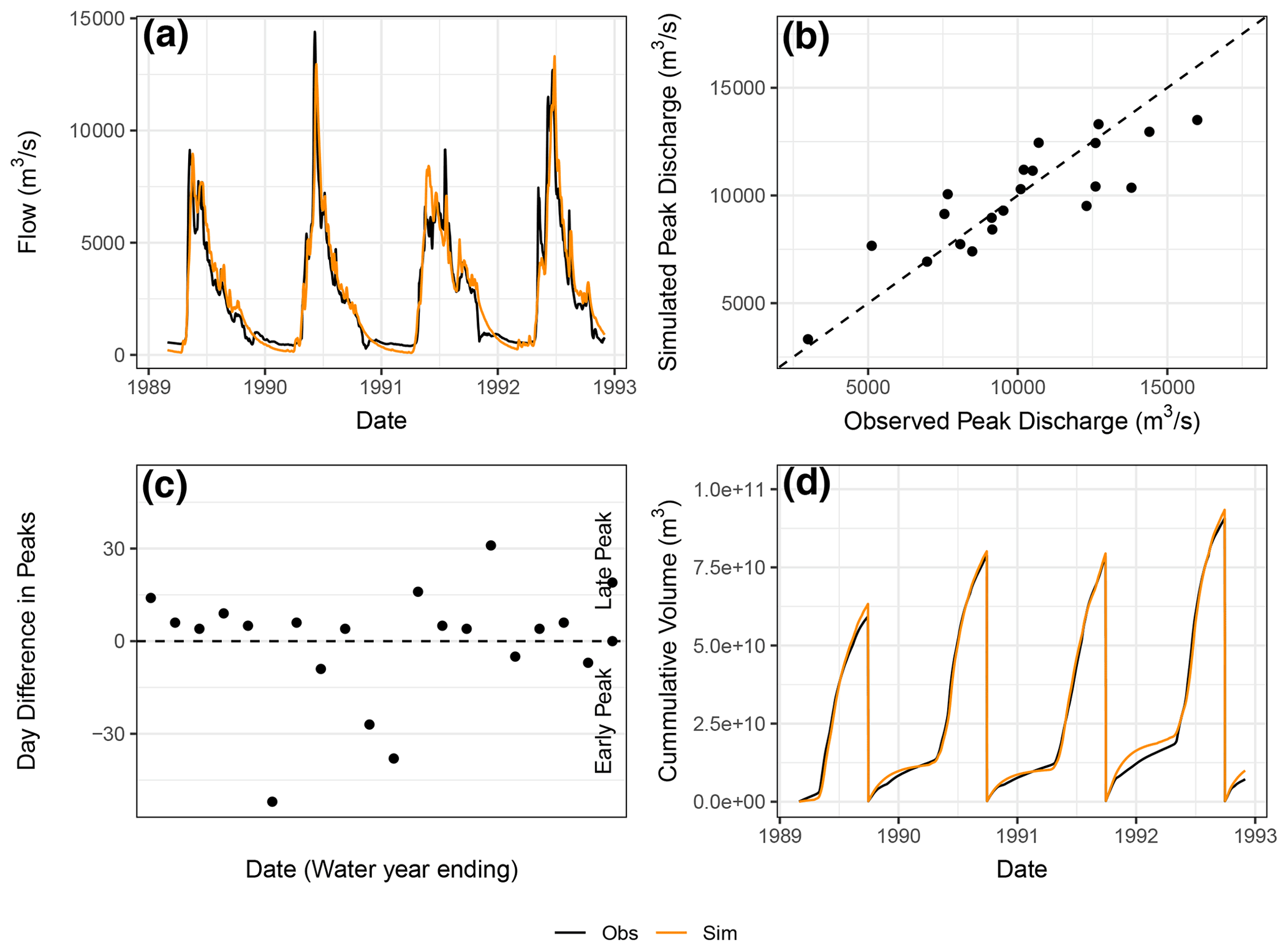
Figure 4Multiple diagnostic plots generated from the RavenR package that may be useful in evaluating model performance: (a) a hydrograph plot for a subset of the simulation period; (b) a scatterplot of simulated and observed annual peak flows; (c) a plot of timing annual peak timing errors; and (d) a plot of cumulative annual flow volumes in time. In plots (a) and (d), the observed value is plotted in black, and the simulated value is plotted in orange.
In Fig. 4a, a simple hydrograph plot for a subset of the simulation period is provided. The hydrograph shows good agreement with respect to the magnitude and timing of summer peaks for the years shown as well as the rising limb of the hydrograph, which was the focus of the calibration in the work of Brown and Craig (2020), with a tendency to overestimate the recession from the peak in June until late December/early January. The underestimation tends to continue until the next peak. The hydrograph is shown for a subset of a few years, allowing for a more critical evaluation of the model performance, as examining the full period can obscure the important deviations of the simulated hydrograph from observations and mask deficiencies. A subset of a hydrograph can also be viewed dynamically as a dygraph in RavenR with the rvn_hyd_dygraph function, which is supported by the dygraphs package (Vanderkam et al., 2018).
The peak flow scatterplot (Fig. 4b) is a plot of the simulated and observed annual peak flows, calculated based on the 1 October water year and produced using the rvn_annual_peak function. This figure provides a visual assessment of the performance of modelled peak flow magnitudes, including any systematic bias in over- or under-predicting peaks as a function of peak magnitude. Here, the model appears to estimate peaks with reasonable performance and without systematic bias, although additional data may be required to produce conclusions that are statistically valid.
While Fig. 4b captures the performance with respect to the magnitude of the flow peaks, the timing of peak flows is not assessed. The plot in Fig. 4c assesses the error in peak timing (rather than magnitude) with the rvn_annual_peak_timing_error function. A perfect model would have all points fall along the zero line, indicating that there is no error in the timing of predicted peaks. The results for the Liard simulation indicate that the model tends to predict peaks slightly later than the observed data, while some of the larger errors in timing tend to be in early peak prediction. In a forecasting framework, a data assimilation technique may reduce the timing (and magnitude) errors that are present in the continuous simulation evaluated here. However, this tendency of the model may still be useful information for forecasters. The use of multiple functions in tandem within RavenR to examine both the peak magnitude and timing errors can be used to evaluate the model performance more comprehensively than a single function (see multiple RavenR functions named as rvn_annual_*).
Finally, Fig. 4d provides a comparison of cumulative flow volumes between the simulated and observed model in time. This plot is generated by the rvn_cum_plot_flow function. The plot for the Liard model shows that the December–March winter period of each year is a time of deviation in cumulative volumes, whereas the freshet-driven summer peak periods tend to match volume quite well overall. This is likely a result of the calibration procedure in Brown and Craig (2020), where ice-affected flows in the winter were not considered in the calibration procedure due to high levels of uncertainty associated with the measurements. Additional functions that examine the relative volumes of simulated and observed flows, but aggregate them rather than examining the differences in time, are the rvn_monthly_vbias and the rvn_annual_volume functions, which provide the monthly average volume differences and the annual volume differences in a scatterplot for each year, respectively. The volume is generally a useful diagnostic metric, as it integrates the modelled hydrograph performance in time and allows the modeller to identify periods of poor cumulative error or systematic errors (e.g., underestimating overall volume) that may be not clear nor obvious when only examining flows.
This paper presented the RavenR package, an R-based set of tools that is designed to support the development, use, and analysis of hydrologic models developed using Raven but can be readily adapted for any hydrologic modelling output. RavenR is a free, open-source software that is intended to support the wealth of options in a flexible modelling framework while maintaining or improving the transparency and reproducibility of the analyses undertaken by the modeller.
The tools within RavenR may be used at any stage of the typical modelling workflow. Although the tools are designed for use with Raven, the analysis and utility functions may be useful in conjunction with any hydrologic model that has similar requirements and workflows to Raven. The RavenR tools provide the means for preparing Raven input files, visualizing and processing input data, executing Raven, and generating a vast array of model checks and performance-related graphics from the Raven output files. All functions in the package are supplemented by additional information and examples (consistent with CRAN requirements), and the package is further accompanied by the introductory documentation in the form of a vignette. This paper illustrates how the RavenR functions may be used in both academic and industrial projects, including generating model input .rvt files, visualizing the model structure, and exploring and assessing the hydrologic model results. This includes aiding the modeller in building an understanding of and trust in the constructed hydrologic model.
A set of RavenR use cases are presented for the Liard River basin, for which a Raven model has previously been built and thoroughly tested (Brown and Craig, 2020). The use cases present how a subset of tools may be used to generate input files for, or analyze the results of, the Raven model of the Liard River basin. The examples are bolstered by an interpretation of the functions and results, which may be useful in interpreting and building confidence in any hydrologic model. The accompanying data repository and code for this paper can fully recreate the figures and analyses presented in the use cases, demonstrating best practices for reproducibility in hydrologic and scientific publications.
Due to the open-source nature of the Raven project, the code is transparent and accessible to users and is being continuously supplemented with new functionalities and improvements. Similarly, the RavenR package is open source and is in active development. It is anticipated that the RavenR project will also continue to improve and expand its functionality in order to meet its goal of supporting Raven users from all backgrounds and experience levels while improving the reproducibility of their work.
The RavenR package is free and open-source software, and the version of the package (v.2.1.4) used to produce the results of this paper is archived on Zenodo: https://doi.org/10.5281/zenodo.5525041 (Chlumsky et al., 2021a). All R code and data used to generate the results and figures presented in this paper are archived on Zenodo at https://doi.org/10.5281/zenodo.5534817 (Chlumsky et al., 2022a) and are also available from GitHub (https://github.com/rchlumsk/RavenR_manuscript_2021, last access: 20 July 2022). The RavenR package is currently available on the Comprehensive R Archive Network (CRAN; https://cran.r-project.org/package=RavenR; Chlumsky et al., 2022b), and the development version of the package is available from Zenodo (https://doi.org/10.5281/zenodo.3468441; Chlumsky et al., 2022c). The Raven hydrologic modelling framework is open source and may be downloaded from http://raven.uwaterloo.ca/ (Craig and the Raven Development Team, 2022).
RC initiated the concept of the RavenR package. RC and JRC contributed the bulk of the package scripts, with contributions and development efforts from all authors. GB and JRC provided the Liard River model files. The use cases were prepared by RC, LS, SGML, SG, and GB. The article was prepared by RC with contributions from all authors.
The contact author has declared that none of the authors has any competing interests.
Publisher's note: Copernicus Publications remains neutral with regard to jurisdictional claims in published maps and institutional affiliations.
The authors would like to thank all those who have contributed to the RavenR project since its inception, including Larry (Haobo) Liu and Joel Trubilowicz. The authors would also like to thank Paul C. Astagneau and the two anonymous reviewers for their comments on improving our manuscript and software.
This research has been supported by the Natural Sciences and Engineering Research Council of Canada (grant no. CGSD3-558879-2021) and the Engineering Excellence Doctoral Fellowship provided at the University of Waterloo.
This paper was edited by Wolfgang Kurtz and reviewed by Paul C. Astagneau and two anonymous referees.
Albers, S.: tidyhydat: Extract and Tidy Canadian Hydrometric Data, J. Open Source Softw., 2, 511, https://doi.org/10.21105/joss.00511, 2017. a
Anderson, E., Chlumsky, R., McCaffrey, D., Trubilowicz, J., Shook, K. R., and Whitfield, P. H.: R-functions for Canadian hydrologists: a Canada-wide collaboration, Can. Water Resour. J., 44, 108–112, 2018. a, b
Astagneau, P. C., Thirel, G., Delaigue, O., Guillaume, J. H. A., Parajka, J., Brauer, C. C., Viglione, A., Buytaert, W., and Beven, K. J.: Technical note: Hydrology modelling R packages – a unified analysis of models and practicalities from a user perspective, Hydrol. Earth Syst. Sci., 25, 3937–3973, https://doi.org/10.5194/hess-25-3937-2021, 2021. a, b
Brown, G. and Craig, J. R.: Structural calibration of an semi-distributed hydrological model of the Liard River basin, Can. Water Resour. J., 45, 287–303, https://doi.org/10.1080/07011784.2020.1803143, 2020. a, b, c, d, e, f, g, h, i
Budyko, M. I.: Climate and life, International Geophysics Series, English ed. edited by: Miller, D. H., Academic Press New York, 18, xvii, 508 p., ISBN 0121394506, 1974. a, b
Chadalawada, J., Herath, H. M. V. V., and Babovic, V.: Hydrologically Informed Machine Learning for Rainfall‐Runoff Modeling: A Genetic Programming‐Based Toolkit for Automatic Model Induction, Water Resour. Res., 56, https://doi.org/10.1029/2019WR026933, 2020. a
Chlumsky, R., Craig, J. R., Brown, G., Scantlebury, L., Grass, S., Lin, S., and Arabzadeh, R.: rchlumsk/RavenR: v2.1.4 release, Zenodo [code], https://doi.org/10.5281/zenodo.5525041, 2021a. a
Chlumsky, R., Mai, J., Craig, J. R., and Tolson, B. A.: Simultaneous Calibration of Hydrologic Model Structure and Parameters Using a Blended Model, Water Resour. Res., 57, e2020WR029229, https://doi.org/10.1029/2020WR029229, 2021b. a, b
Chlumsky, R., Craig, J. R., Brown, G., Scantlebury, L., Grass, S., Lin, S., and Arabzadeh, R.: rchlumsk/RavenR_manuscript_2021: Initial pre-release v0.2, Zenodo [data set], https://doi.org/10.5281/zenodo.6421692, 2022a. a, b
Chlumsky, R., Craig, J. R., Scantlebury, L., Lin, S., Grass, S., Brown, G., and Arabzadeh, R.: RavenR: Raven Hydrological Modelling Framework R Support and Analysis, R package version 2.1.9, https://cran.r-project.org/package=RavenR, last access: 20 July 2022b. a
Chlumsky, R., Craig, J. R., Scantlebury, L., Lin, S., Grass, S., Brown, G., and Arabzadeh, R.: rchlumsk/RavenR: latest release, Zenodo [code], https://doi.org/10.5281/zenodo.3468441, 2022c. a
Clark, M. P., Slater, A. G., Rupp, D. E., Woods, R. A., Vrugt, J. A., Gupta, H. V., Wagener, T., and Hay, L. E.: Framework for Understanding Structural Errors (FUSE): A modular framework to diagnose differences between hydrological models, Water Resour. Rese., 44, 12, https://doi.org/10.1029/2007WR006735, 2008. a
Clark, M. P., Kavetski, D., and Fenicia, F.: Pursuing the method of multiple working hypotheses for hydrological modeling, Water Resour. Res., 47, 9, https://doi.org/10.1029/2010WR009827, 2011. a
Clark, M. P., Nijssen, B., Lundquist, J. D., Kavetski, D., Rupp, D. E., Woods, R. A., Freer, J. E., Gutmann, E. D., Wood, A. W., Brekke, L. D., Arnold, J. R., Gochis, D. J., and Rasmussen, R. M.: A unified approach for process-based hydrologic modeling: 1. Modeling concept, Water Resour. Res., 51, 2498–2514, 2015. a
Coxon, G., Freer, J., Lane, R., Dunne, T., Knoben, W. J. M., Howden, N. J. K., Quinn, N., Wagener, T., and Woods, R.: DECIPHeR v1: Dynamic fluxEs and ConnectIvity for Predictions of HydRology, Geosci. Model Dev., 12, 2285–2306, https://doi.org/10.5194/gmd-12-2285-2019, 2019. a
Craig, J. R. and the Raven Development Team: Raven: User's and Developer's Manual v3.5, http://raven.uwaterloo.ca/, last access: 20 July 2022. a, b, c, d, e, f
Craig, J. R., Brown, G., Chlumsky, R., Jenkinson, R. W., Jost, G., Lee, K., Mai, J., Serrer, M., Sgro, N., Shafii, M., Snowdon, A. P., and Tolson, B. A.: Flexible watershed simulation with the Raven hydrological modelling framework, Environ. Modell. Softw., 129, https://doi.org/10.1016/j.envsoft.2020.104728, 2020. a, b, c, d, e
Csardi, G. and Nepusz, T.: The igraph software package for complex network research, InterJournal, Complex Systems, 1695, http://igraph.org (last access: 20 July 2022), 2006. a
Dal Molin, M., Kavetski, D., and Fenicia, F.: SuperflexPy 1.3.0: an open-source Python framework for building, testing, and improving conceptual hydrological models, Geosci. Model Dev., 14, 7047–7072, https://doi.org/10.5194/gmd-14-7047-2021, 2021. a
Euser, T., Winsemius, H. C., Hrachowitz, M., Fenicia, F., Uhlenbrook, S., and Savenije, H. H. G.: A framework to assess the realism of model structures using hydrological signatures, Hydrol. Earth Syst. Sci., 17, 1893–1912, https://doi.org/10.5194/hess-17-1893-2013, 2013. a
Fenicia, F., Savenije, H. H. G., Matgen, P., and Pfister, L.: Understanding catchment behavior through stepwise model concept improvement, Water Resour. Res., 44, 1, https://doi.org/10.1029/2006WR005563, 2008. a
Fenicia, F., Kavetski, D., and Savenije, H. H. G.: Elements of a flexible approach for conceptual hydrological modeling: 1. Motivation and theoretical development, Water Resour. Res., 47, 11, https://doi.org/10.1029/2010WR010174, 2011. a
Grolemund, G. and Wickham, H.: Dates and Times Made Easy with lubridate, J. Stat. Softw., 40, 1–25, https://doi.org/10.18637/jss.v040.i03, 2011. a
Gupta, H. V., Kling, H., Yilmaz, K. K., and Martinez, G. F.: Decomposition of the mean squared error and NSE performance criteria: Implications for improving hydrological modelling, J. Hydrol., 377, 80–91, https://doi.org/10.1016/j.jhydrol.2009.08.003, 2009. a
Hoey, S. V., Seuntjens, P., van Der Kwast, J., and Nopens, I.: A qualitative model structure sensitivity analysis method to support model selection, J. Hydrol., 519, 3426–3435, https://doi.org/10.1016/j.jhydrol.2014.09.052, 2014. a
Hutton, C., Wagener, T., Freer, J., Han, D., Duffy, C., and Arheimer, B.: Most computational hydrology is not reproducible, so is it really science?, Water Resour. Res., 52, 7548–7555, https://doi.org/10.1002/2016WR019285, 2016. a
Jackson, E. K., Roberts, W., Nelsen, B., Williams, G. P., Nelson, E. J., and Ames, D. P.: Introductory overview: Error metrics for hydrologic modelling – A review of common practices and an open source library to facilitate use and adoption, Environ. Modell. Softw., 119, 32–48, https://doi.org/10.1016/j.envsoft.2019.05.001, 2019. a
Kavetski, D. and Fenicia, F.: Elements of a flexible approach for conceptual hydrological modeling: 2. Application and experimental insights, Water Resour. Res., 47, 11, https://doi.org/10.1029/2011WR010748, 2011. a
Knoben, W. J. M., Freer, J. E., Fowler, K. J. A., Peel, M. C., and Woods, R. A.: Modular Assessment of Rainfall–Runoff Models Toolbox (MARRMoT) v1.2: an open-source, extendable framework providing implementations of 46 conceptual hydrologic models as continuous state-space formulations, Geosci. Model Dev., 12, 2463–2480, https://doi.org/10.5194/gmd-12-2463-2019, 2019. a
Knoben, W. J. M., Freer, J. E., Peel, M. C., Fowler, K. J. A., and Woods, R. A.: A brief analysis of conceptual model structure uncertainty using 36 models and 559 catchments, Water Resour. Res., 56, 9, https://doi.org/10.1029/2019WR025975, 2020. a
LaZerte, S. E. and Albers, S.: weathercan: Download and format weather data from Environment and Climate Change Canada, J. Open Source Softw., 3, 571, https://doi.org/10.21105/joss.00571, 2018. a
Leavesley, G. H., Markstrom, S. L., Restrepo, P. J., and Viger, R. J.: A modular approach to addressing model design, scale, and parameter estimation issues in distributed hydrological modelling, Hydrol. Process., 16, 173–187, 2002. a
Mai, J., Craig, J. R., and Tolson, B. A.: Simultaneously determining global sensitivities of model parameters and model structure, Hydrol. Earth Syst. Sci., 24, 5835–5858, https://doi.org/10.5194/hess-24-5835-2020, 2020. a, b
McLaughlin, D. L., Kaplan, D. A., and Cohen, M. J.: A significant nexus: Geographically isolated wetlands influence landscape hydrology, Water Resour. Res., 50, 7153–7166, https://doi.org/10.1002/2013WR015002, 2014. a
Nash, J. E. and Sutcliffe, J. V.: River flow forecasting through conceptual models part I – A discussion of principles, J. Hydrol., 10, 282–290, https://doi.org/10.1016/0022-1694(70)90255-6, 1970. a
Orellana, B., Pechlivanidis, I., Mcintyre, N., Wheater, H., and Wagener, T.: A Toolbox for the Identification of Parsimonious Semi-Distributed Rainfall-Runoff Models: Application to the Upper Lee Catchment, in: International Congress on Environmental Modelling and Software, https://scholarsarchive.byu.edu/cgi/viewcontent.cgi?article=2723&context=iemssconference (last access: 15 September 2021), 2008. a
Perrin, C., Michel, C., and Andréassian, V.: Improvement of a parsimonious model for streamflow simulation, J. Hydrol., 279, 275–289, 2003. a
Pilz, T., Francke, T., Baroni, G., and Bronstert, A.: How to Tailor my Process‐based Hydrological Model? Dynamic Identifiability Analysis of Flexible Model Structures, Water Resour. Res., 56, 8, https://doi.org/10.1029/2020WR028042, 2020. a
R Core Team: R: A Language and Environment for Statistical Computing, R Foundation for Statistical Computing, Vienna, Austria, https://www.R-project.org/ (last access: 15 September 2021), 2021. a
Remmers, J. O., Teuling, A. J., and Melsen, L. A.: Can model structure families be inferred from model output?, Environ. Model. Softw., 133, 104817, https://doi.org/10.1016/j.envsoft.2020.104817, 2020. a
Ryan, J. A. and Ulrich, J. M.: xts: eXtensible Time Series, r package version 0.12.1, https://CRAN.R-project.org/package=xts (last access: 15 September 2022), 2020. a
Slater, L. J., Thirel, G., Harrigan, S., Delaigue, O., Hurley, A., Khouakhi, A., Prosdocimi, I., Vitolo, C., and Smith, K.: Using R in hydrology: a review of recent developments and future directions, Hydrol. Earth Syst. Sci., 23, 2939–2963, https://doi.org/10.5194/hess-23-2939-2019, 2019. a, b
Spieler, D., Mai, J., Craig, J. R., Tolson, B. A., and Schütze, N.: Automatic Model Structure Identification for Conceptual Hydrologic Models, Water Resour. Res., 56, 9, https://doi.org/10.1029/2019WR027009, 2020. a, b
Stroustrup, B.: The C++ programming language, Addison-Wesley, Upper Saddle River, NJ, 4th Edn., ISBN 978-0321563842, 2013. a
Van Rossum, G. and Drake, F. L.: Python 3 Reference Manual, CreateSpace, Scotts Valley, CA, ISBN 1441412697, 2009. a
Vanderkam, D., Allaire, J., Owen, J., Gromer, D., and Thieurmel, B.: dygraphs: Interface to “Dygraphs” Interactive Time Series Charting Library, r package version 1.1.1.6, https://CRAN.R-project.org/package=dygraphs (last access: 15 September 2021), 2018. a
Vereecken, H., Huisman, J. A., Hendricks Franssen, H. J., Brüggemann, N., Bogena, H. R., Kollet, S., Javaux, M., van der Kruk, J., and Vanderborght, J.: Soil hydrology: Recent methodological advances, challenges, and perspectives, Water Resour. Res., 51, 2616–2633, https://doi.org/10.1002/2014WR016852, 2015. a
Wickham, H.: ggplot2: Elegant Graphics for Data Analysis, Springer-Verlag New York, https://ggplot2.tidyverse.org (last access: 15 September 2021), 2016. a
Wickham, H.: tidyr: Tidy Messy Data, r package version 1.1.3, https://CRAN.R-project.org/package=tidyr (last access: 15 September 2021), 2021. a
Wickham, H., François, R., Henry, L., and Müller, K.: dplyr: A Grammar of Data Manipulation, r package version 1.0.5, https://CRAN.R-project.org/package=dplyr (last access: 15 September 2021), 2021a. a
Wickham, H., Hester, J., and Chang, W.: devtools: Tools to Make Developing R Packages Easier, r package version 2.4.0, https://CRAN.R-project.org/package=devtools (last access: 15 September 2021), 2021b. a
Zambrano-Bigiarini, M.: hydroGOF: Goodness-of-fit functions for comparison of simulated and observed hydrological time series, r package version 0.4-0, Zenodo [code], https://doi.org/10.5281/zenodo.839854, 2020. a