the Creative Commons Attribution 4.0 License.
the Creative Commons Attribution 4.0 License.
 | 16 Sep 2022
The ICON-A model for direct QBO simulations on GPUs (version icon-cscs:baf28a514)
Marco A. Giorgetta
William Sawyer
Xavier Lapillonne
Panagiotis Adamidis
Dmitry Alexeev
Valentin Clément
Remo Dietlicher
Jan Frederik Engels
Monika Esch
Henning Franke
Claudia Frauen
Walter M. Hannah
Benjamin R. Hillman
Luis Kornblueh
Philippe Marti
Matthew R. Norman
Robert Pincus
Sebastian Rast
Daniel Reinert
Reiner Schnur
Uwe Schulzweida
Bjorn Stevens
Classical numerical models for the global atmosphere, as used for numerical weather forecasting or climate research, have been developed for conventional central processing unit (CPU) architectures. This hinders the employment of such models on current top-performing supercomputers, which achieve their computing power with hybrid architectures, mostly using graphics processing units (GPUs). Thus also scientific applications of such models are restricted to the lesser computer power of CPUs. Here we present the development of a GPU-enabled version of the ICON atmosphere model (ICON-A), motivated by a research project on the quasi-biennial oscillation (QBO), a global-scale wind oscillation in the equatorial stratosphere that depends on a broad spectrum of atmospheric waves, which originates from tropical deep convection. Resolving the relevant scales, from a few kilometers to the size of the globe, is a formidable computational problem, which can only be realized now on top-performing supercomputers. This motivated porting ICON-A, in the specific configuration needed for the research project, in a first step to the GPU architecture of the Piz Daint computer at the Swiss National Supercomputing Centre and in a second step to the JUWELS Booster computer at the Forschungszentrum Jülich. On Piz Daint, the ported code achieves a single-node GPU vs. CPU speedup factor of 6.4 and allows for global experiments at a horizontal resolution of 5 km on 1024 computing nodes with 1 GPU per node with a turnover of 48 simulated days per day. On JUWELS Booster, the more modern hardware in combination with an upgraded code base allows for simulations at the same resolution on 128 computing nodes with 4 GPUs per node and a turnover of 133 simulated days per day. Additionally, the code still remains functional on CPUs, as is demonstrated by additional experiments on the Levante compute system at the German Climate Computing Center. While the application shows good weak scaling over the tested 16-fold increase in grid size and node count, making also higher resolved global simulations possible, the strong scaling on GPUs is relatively poor, which limits the options to increase turnover with more nodes. Initial experiments demonstrate that the ICON-A model can simulate downward-propagating QBO jets, which are driven by wave–mean flow interaction.
- Article
(6538 KB) - Full-text XML
- BibTeX
- EndNote


Numerical weather prediction (NWP) and climate research make use of numerical models which solve discretized equations for fluid dynamics on the globe. For NWP and many research applications, the resolution is chosen as high as possible for the available computing resources. Higher resolution allows atmospheric processes to be explicitly computed over a larger range of scales and thus the dynamics of the global atmosphere to be computed more faithfully. Examples of small-scale features, which are relevant for NWP or climate research, are cumulus clouds, gravity waves generated by orographic obstacles and convective clouds, or turbulent motions in the boundary layer. The advantages of higher resolution, however, come at higher costs and especially longer time to solution, which practically limits the maximum resolution that can be afforded in specific applications. In climate research, most global simulations of the atmospheric circulations still use resolutions of a few tens of kilometers to about 200 km for simulations over decades to centuries. But the most ambitious global simulations now already reach resolutions of just a few kilometers (Stevens et al., 2019), which means that basic structures of tropical deep convection can be computed explicitly. Such simulations are still the exception and limited to short time periods, owing to the slow turnover in terms of simulated time per wall clock time unit. A specific reason for the limitation of such simulations in resolution or simulated time is that the computing codes of these numerical models have been developed and optimized for conventional central processing unit (CPU) architectures, while the most advanced and powerful computer systems now employ hybrid architectures with graphics processing units (GPUs). Thus, the most powerful computing systems are effectively out of reach for most existing computing codes for numerical weather prediction and climate research.
This also holds for the ICON model system, which has been developed since the early 2000s for use on either cache-based or vectorizing CPUs, with components for atmosphere, land, and ocean. The buildup of the hybrid Piz Daint compute system at the Swiss National Supercomputing Centre, however, created a strong motivation to port the ICON model to GPUs in order to benefit from the immense compute power of Piz Daint resulting from up to 5704 GPUs. With this motivation, it was decided to port the atmospheric component of ICON (ICON-A) in two specific configurations to GPUs so that the development effort can be limited initially to a subset of the ICON codes. The model configuration in the focus of the presented work was designed for the “Quasi-biennial oscillation in a changing climate” (QUBICC) project, for which global simulations at horizontal resolutions of 5 km or better and vertical resolutions of a few hundred meters up to the middle stratosphere are planned to investigate the dynamics of the quasi-biennial oscillation (QBO), a global-scale zonal wind oscillation in the equatorial stratosphere, for which the main characteristics are reviewed in Baldwin et al. (2001), and an overview of the QBO impacts is given in Anstey et al. (2022). Using this very high resolution is essential for the QUBICC project so that the dynamical links from small-scale and quickly evolving tropical deep convection to the global-scale and slowly varying wind system of the QBO can be directly computed. This makes a substantial difference to existing simulations of the QBO in coarser models, where deep convection and the related gravity wave effects must be parameterized. The uncertainty in the parameterization of convection and gravity waves, as necessary in coarser models, is the main reason for problems in simulating the QBO (Schirber et al., 2015; Richter et al., 2020).
Until now, only a few attempts have been made to port general circulation models for the atmosphere or the ocean to GPUs, using different methods. Demeshko et al. (2013) presented an early attempt, in which only the most costly part of the NICAM model, the horizontal dynamics, was ported to GPUs, for which these parts were reprogrammed in CUDA Fortran. Fuhrer et al. (2018) ported the COSMO5 limited area model to GPUs by using directives and by rewriting the dynamical core from Fortran to C++ and employing the domain-specific language STELLA. Similarly, Wang et al. (2021) ported their LICOM3 model by rewriting the code in the time loop from Fortran to C and further to HIP. In the case of the NIM weather model, Govett et al. (2017), however, decided to work with directives only so that the same code can be used on CPU, GPU, and Many Integrated Core (MIC) processors. Other models have partial GPU implementations, such as WRF (Huang et al., 2015), in CUDA-C and MPAS (Kim et al., 2021), with OpenACC. In our attempt, after initial steps described later, it was decided to stay with the standard ICON Fortran code wherever possible and thus to work with directives, so that ICON-A works on CPUs and GPUs. In the CPU case, applications shall continue to use the proven parallelization by MPI domain decomposition mixed with OpenMP multi-threading, while in the GPU case, parallelization should now combine the MPI domain decomposition with OpenACC directives for the parallelization on the GPU. OpenACC was chosen because this was the only practical option on the GPU compute systems used in the presented work and described below. Specifically OpenMP version 5 was not available on these systems. Consequently the resulting ICON code presented here now includes OpenMP and OpenACC directives.
In the following, we present the model configuration for QUBICC experiments, for which the ICON-A model has been ported to GPUs (Sect. 2), the relevant characteristics of the compute systems Piz Daint, JUWELS Booster and Levante used in this study (Sect. 3), the methods used for porting ICON codes to GPUs (Sect. 4), the validation methods used to detect porting errors (Sect. 5), the results from benchmarking on the three compute systems (Sect. 6), selected results from first QUBICC experiments (Sect. 7), and the conclusions.
The QUBICC experiments make use of very high resolution grids, on which dynamics and transport are explicitly solved. This means that only a small number of processes need to be parameterized in comparison to the low-resolution simulations presented by Giorgetta et al. (2018). This reduced physics package, which we call Sapphire physics, comprises parameterizations for radiation, vertical turbulent diffusion, and cloud microphysics in the atmosphere, and land surface physics, as detailed in Sect. 2.5. Thus the model components to be ported to GPU include dynamics, transport, the aforementioned physics parameterizations, and additionally the essential infrastructure components for memory and communication. The following subsections provide more details on the model grids defining the resolution and the components computed on these grids.
2.1 Horizontal grid
The horizontal resolution needs to be high enough to allow for the explicit simulation of tropical deep convection, and at the same time simulation costs must be limited to realistic amounts, as every doubling of the horizontal resolution multiplies the computing costs by a factor of 8, resulting from a factor 2 for each horizontal dimension and a factor 2 for the necessary shortening of the time step. From earlier work made with ICON-A, it is understood that Δx=5 km is the smallest resolution, for which deep convection is simulated in an acceptable manner (Hohenegger et al., 2020) and for which realistic gravity wave spectra related to the resolved convection can be diagnosed (Müller et al., 2018; Stephan et al., 2019). As any substantial increase in horizontal resolution is considered to exceed the expected compute time budget, a horizontal mean resolution of Δx=5 km is used, as available on the R2B9 grid of the ICON model; see Table 1 in Giorgetta et al. (2018). The specific ICON grid ID is 0015, referring to a north–south symmetric grid, which results from a 36∘ longitudinal rotation of the southern hemispheric part of the ICON grid after the initial R2 root bisection of the spherical icosahedron. (Older setups as in Giorgetta et al., 2018 did not yet use the rotation step for a north–south symmetric grid.)
2.2 Vertical grid
The vertical grid of the ICON-A model is defined by a generalized smooth-level vertical coordinate (Leuenberger et al., 2010) formulated in geometric height above the reference ellipsoid, which is assumed to be a sphere. At the height of 22.5 km, the model levels transition to levels of constant height, which are levels of constant geopotential as well. For the QUBICC experiments, a vertical grid is chosen that has 191 levels between the surface and the model top at a height of 83 km. This vertical extension and resolution is chosen as a compromise between a number of factors:
-
A high vertical resolution is needed to represent the dynamics of vertically propagating waves, considering waves which can be resolved horizontally. The resolution should also be sufficient in the shear layers of the QBO, where the Doppler shifting shortens the vertical wavelengths of upward-propagating waves, with phase speeds similar to the velocity of the mean flow in the shear layer. Typically, a vertical resolution of a few hundred meters is wanted.
-
The vertical extent of the model should be high enough to allow for the simulation of the QBO in the tropical stratosphere without direct numerical impacts from the layers near the model top, where numerical damping is necessary to avoid numerical artifacts. In practice the ICON model uses the upper boundary condition of zero vertical wind, w=0, and applies a Rayleigh damping on the vertical wind (Klemp et al., 2008). This damping starts above a given minimum height from where it is applied up to the top of the model, using a tanh vertical scaling function that changes from 0 at the minimum height to 1 at the top of the model (Zängl et al., 2015). Based on experience, the depth of the damped layer should be ca. 30 km. Combining this with the stratopause height of ca. 50 km, a top height of ca. 80 km is needed.
-
A further constraint is the physical validity of the model formulation. The key limitation consists in the radiation scheme RTE+RRTMGP, which is developed and validated for conditions of local thermal equilibrium (LTE) between the vibrational levels of the molecules involved in radiative transitions and the surrounding medium. This limits the application of this radiation scheme to levels below atmospheric pressures of 0.01 hPa. The atmospheric pressure of 0.01 hPa corresponds to a height of ca. 80 km with a few kilometers' variation depending on season, latitude and weather. Other complications existing at higher altitudes, besides non-LTE, are strong tides and processes which are not represented in the model, for instance, atmospheric chemistry and effects from the ionized atmosphere. Such complications shall be avoided in the targeted model setup.
-
Computational cost increases approximately linearly with the number of layers. Thus, fewer layers would allow for more or longer simulations at the same costs.
As a compromise, a vertical grid is chosen that has 191 levels between the surface and the model top at a height of 83 km. The first layer above the surface has a constant thickness of 40 m. Between this layer and a height of 22.5 km, the height of the model levels and thus the layer thicknesses vary following the implemented smooth-level algorithm. Above 22.5 km, all remaining model levels are levels of constant height. The resulting profile of layer thickness versus layer height is shown in Fig. 1 for a surface point at sea level (blue profile) and the highest surface point on the R2B9 grid, which is in the Himalayas and has a height of 7368 m (red profile). The vertical resolution ranges from 300 m at 12 km near the tropopause to 600 m at 50 km height near the stratopause. Over high terrain, however, a relatively strong change in vertical resolution appears near 13 km height, which unfortunately cannot be avoided with the existing implementation of the smooth-level algorithm.

Figure 1Level height vs. layer thickness from the surface to the model top for a surface height of 0 m over ocean (blue) and for the highest surface point of the R2B9 grid at 7368 m at N, E in the Himalayas (red). The lowermost layer has a constant thickness of 40 m and thus is centered at 20 m height above the surface. The uppermost layer is centered at 82 361 m and has an upper bound at 83 000 m. At heights above 22 500 m, the vertical resolution profile is independent of the surface height.
2.3 Dynamics
The horizontally explicit and only vertically implicit numerics of the ICON-A dynamical core requires generally short time steps for numerical stability of the dynamics. The necessity to use very short model time steps is however alleviated by splitting the model time step into a typically small number of dynamics sub-steps, each solved by a predictor–corrector method, as detailed in Zängl et al. (2015). The explicit vertical numerics of the tracer transport scheme (Reinert, 2020) may add further constraints on the model time step if levels are thin or the vertical velocity large. For satisfying both, the QUBICC experiments operate with five dynamics sub-steps and a model time step of , where dtdyn=8 s is the time step of the dynamics sub-steps. The model time step is thus slightly shorter than the 45 s time step used for the same horizontal resolution in Hohenegger et al. (2020). The reason is the increased vertical resolution, which imposes narrower limits for stability in the vertical tracer transport.
2.4 Tracer transport
The QUBICC experiments include a total of six tracers for water vapor, cloud water, cloud ice, rain, snow, and graupel. This enlarged set of tracers compared to Giorgetta et al. (2018) is related to the more detailed cloud microphysics scheme that predicts also rain, snow, and graupel; see below. For efficiency reasons, the transport of hydrometeors, i.e., cloud water, cloud ice, rain, snow and graupel, is limited to heights below 22.5 km, assuming that none of these hydrometeors exist in the vicinity of this stratospheric height level and above. Concerning the configuration of the transport scheme (Reinert, 2020), the horizontal advection for water vapor has been changed from a combination of a semi-Lagrangian flux form and a third-order Miura scheme with sub-cycling to a second-order Miura scheme with sub-cycling. The choice of the simpler scheme is related to the difficulty of a GPU implementation for a semi-Lagrangian flux form scheme. (The GPU port of this scheme is currently ongoing.) Sub-cycling means that the integration from time step n to n+1 is split into three sub-steps to meet the stability requirements. This sub-cycling is applied only above 22.5 km height, i.e., in the stratosphere and mesosphere, where strong winds exist. The other tracers, the hydrometeors, are also transported with the second-order Miura scheme, though without sub-cycling because they are not transported above 22.5 km.
2.5 Physics
The QUBICC experiments make use of the Sapphire physics package for storm-resolving simulations. This package deviates from the ECHAM-based physics package described in Giorgetta et al. (2018) in a number of points. First of all, the physics package excludes parameterizations for convection, atmospheric, and orographic gravity waves and other sub-grid-scale orographic effects. These processes are mostly resolved, though not completely, at the grid resolutions used in QUBICC experiments. Further, the scientific goal of the QUBICC experiments includes the investigation of the QBO forcing based on the resolved dynamics of deep convective clouds and related waves, which can be granted by excluding parameterized representations of these processes. As a result, the Sapphire physics package is considerably smaller and the model structurally simplified.
The atmospheric processes which still require parameterizations are radiation, the vertical diffusion related to unresolved eddies, and the cloud microphysics. Additionally, land processes must be parameterized for the interactive representation of the lower atmospheric boundary conditions over land.
2.5.1 Radiation
From the beginning of the GPU port, it was clear that the radiation code was a special challenge due to its additional dimension in spectral space that resolves the shortwave and longwave spectra. Further, initial work on the original PSRAD radiation scheme (Pincus and Stevens, 2013) showed that a substantial refactoring would have been necessary for a well-performing GPU version of PSRAD, with an uncertain outcome. Therefore the decision was taken to replace PSRAD by the new RTE+RRTMGP radiation code (Pincus et al., 2019), which was designed from the beginning to work efficiently on CPUs and GPUs, with separate code kernels for each architecture. Thus the ICON code for QUBICC now employs the RTE+RRTMGP code. From a modeling point of view RTE+RRTMGP employs the same spectral discretization methods as PSRAD, namely the k-distribution method and the correlated-k approximation. Differences exist however in using absorption coefficients from more recent spectroscopic data in RTE+RRTMGP and in the number and distribution of discretization points, so-called g-points, in the SW and LW spectra. While PSRAD used 252 g-points (140 in the longwave spectral region and 112 in the shortwave), RTE+RRTMGP versions on Piz Daint and JUWELS Booster use 480 (256 LW + 224 SW) and 240 (128 LW + 112 SW) g-points, respectively. Scattering of longwave radiation by cloud particles is not activated in RTE+RRTMGP, so that also in this aspect it is equivalent to the older PSRAD scheme.
As the calculations for the radiative transfer remain the most expensive portion of the model system, a reduced calling frequency, as common in climate and numerical weather prediction models, remains necessary. For QUBICC experiments, the radiation time step is set to , thus a bit shorter and more frequent than in the simulations of Hohenegger et al. (2020), where was used.
Concerning the atmospheric composition, the radiative transfer depends on prognostic fields for water vapor, cloud water, and cloud ice and on externally specified time-dependent greenhouse gas concentrations for CO2, CH4, N2O, CFC11, and CFC12 and O3, as prepared for the historical simulations of CMIP6 (Meinshausen et al., 2017).
In the spirit of allowing for only explicitly modeled scales, all tracers used in the radiation are assumed to be homogeneous within each cell. Thus no parameterized effect of cloud inhomogeneities on the optical path of cloud water and cloud ice is applied in the QUBICC simulations.
Rain, snow, and graupel concentrations are neglected in the radiative transfer, and for practical reasons no aerosol forcing has been used in the initial experiments.
2.5.2 Vertical diffusion
For the representation of the vertical turbulent diffusion of heat, momentum and tracers, the total turbulent energy parameterization of Mauritsen et al. (2007) is used, which is implicitly coupled to the land surface scheme; see below.
2.5.3 Land surface physics
Land processes in ICON-A are parameterized in the JSBACH land surface model, which provides the lower boundary conditions for the atmosphere and is implicitly coupled to the atmospheric vertical diffusion parameterization. The infrastructure, ICON-Land, for this ICON-A land component has been newly designed in a Fortran2008 object-oriented, modular, and flexible way. The specific implementations of physical, biogeophysical, and biogeochemical processes constituting the JSBACH model have been ported from the JSBACH version used with the MPIESM/ECHAM modeling framework (Reick et al., 2021; Stevens et al., 2013).
For the experiments described in this study, JSBACH has been used in a simplified configuration that uses only the physical processes and in which the sub-grid-scale heterogeneity of the land surface properties in each grid box is described by lakes, glaciers, and only one single vegetated tile, as in ICON-A (Giorgetta et al., 2018).
2.5.4 Cloud microphysics
Cloud microphysics is parameterized by the “graupel” microphysics scheme (Sect. 5.2 and 5.3, Doms et al., 2011), which is a single-moment microphysics scheme for water vapor, cloud water, cloud ice, rain, snow, and graupel. All hydrometeors are also transported. For efficiency reasons, the computation of cloud microphysics and the transport of cloud tracers are limited to heights below 22.5 km height.
2.5.5 Cloud cover
In the spirit of allowing for only explicitly modeled scales, it is assumed that all fields controlling cloud condensation and thus cloud cover are homogeneous in each cell. Thus the instantaneous cloud cover in a cell is diagnosed as either 0 % or 100 %, depending on the cloud condensate mass fraction exceeding a threshold value of 10−6 kg kg−1. Total cloud cover in a column thus is either 0 % or 100 %.
2.6 Coupling of processes
The coupling of the processes described above and the transformations between dynamics variables and physics variables, as well as the time integration, closely follow the setup of Giorgetta et al. (2018) described in Sect. 3, also using the simplified case of their Eq. (8), for which the scheme is displayed in Fig. 2. However, a difference with respect to Giorgetta et al. (2018) consists in the coupling between the physical parameterizations and is shown in Fig. 3. The coupling scheme applied in our study couples radiation, vertical diffusion with surface land physics, and cloud microphysics sequentially instead of using a mixed coupling scheme (cf. Fig. 6 of Giorgetta et al., 2018).
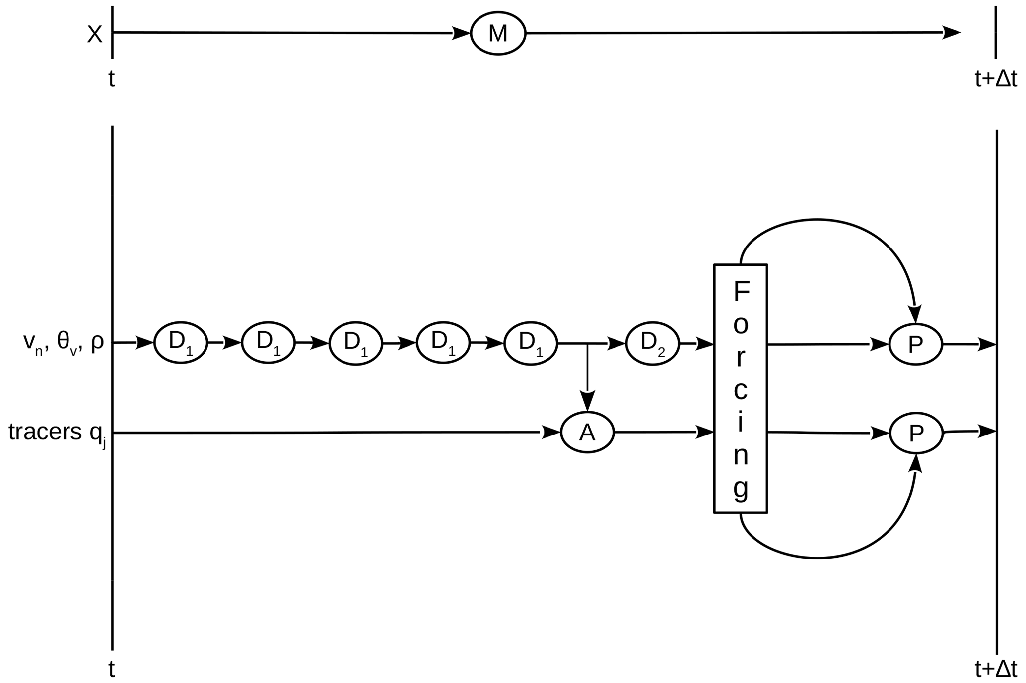
Figure 2The model operator M propagates the model state X from time t to t+dt, with X consisting of the variables vn,θv and ρ, which are processed by the dynamics, and tracer mass fractions qi, which are processed by the advection scheme A. The dynamics consists of a sequence of five sub-steps (D1), each propagating the dynamics variables by , followed by horizontal diffusion (D2). The advection makes use of the air mass flux computed in the dynamics to achieve consistency with continuity. The intermediate state resulting from dynamics and advection is used for the computation of the forcing, which is applied in the physics update (P) that produces the new state X(t+dt).
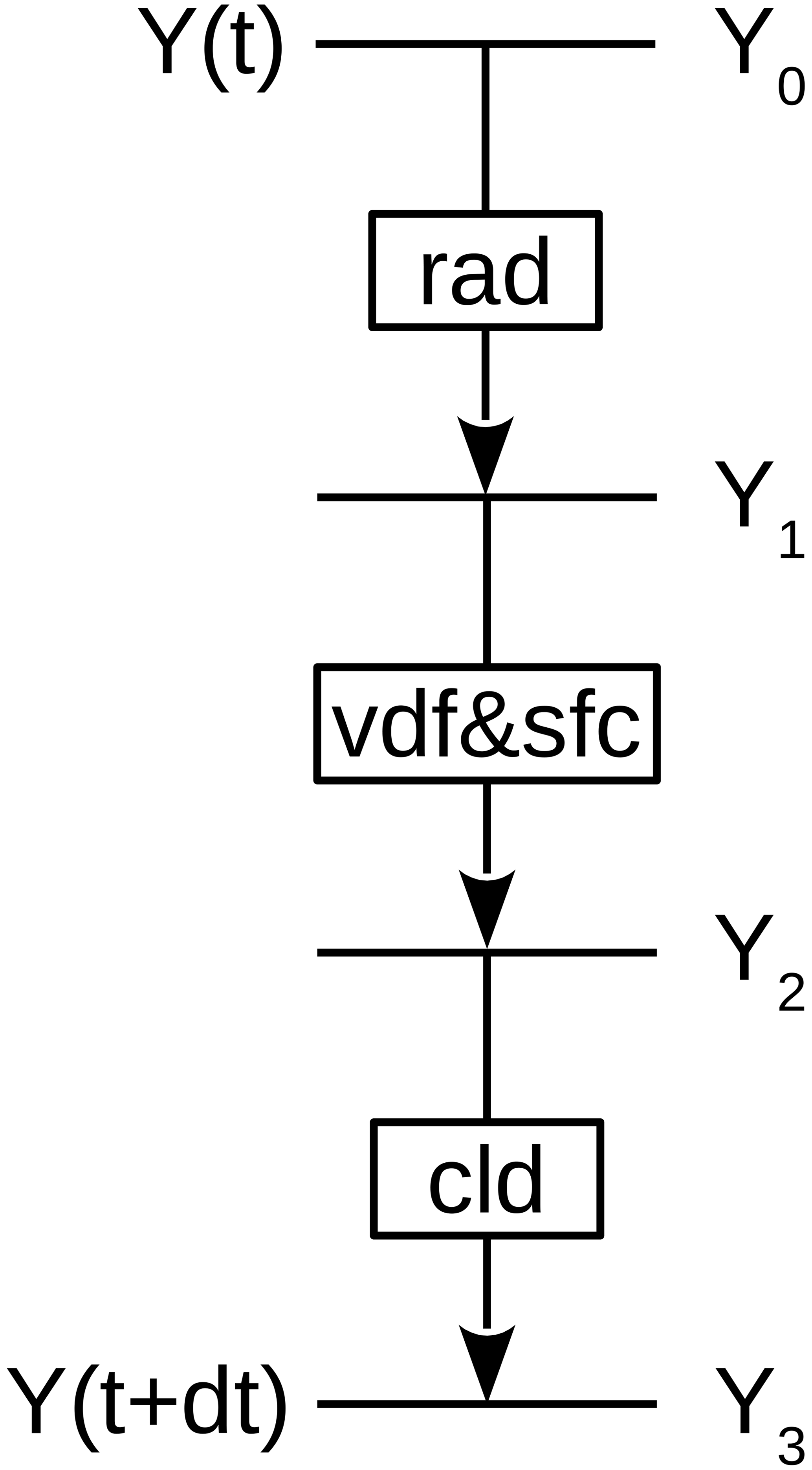
Figure 3The forcing consists of three sequentially coupled components for radiative heating (rad), vertical diffusion (vdf) coupled implicitly to land surface processes (sfc), and cloud microphysics (cld). Each component computes its contribution to the forcing from a provisional state Y expressed in the physics variables , and v.
In this section the compute systems used for the presented work are described briefly, with Piz Daint at the Swiss National Supercomputing Centre (CSCS) being the main system where the GPU port of ICON was developed, and experiments have been carried out during the first year of a PRACE allocation. The second-year PRACE allocation was shifted to JUWELS Booster at the Forschungszentrum Jülich (FZJ), where the GPU port of ICON was further optimized followed by new scaling tests and experiments. Last but not least the same code was used also for additional scaling tests on the new Levante computer at the German Climate Computing Center (DKRZ), which is a CPU architecture, thus demonstrating the portability across a number of platforms. The maximum sustained throughput Rmax from the HPL (high-performance LINPACK) benchmarks is used to normalize the performance across the machines. Because ICON is often memory-bandwidth-limited, the HPCG (high-performance conjugate gradient) benchmarks would be a more informative norm; however these are not available for Levante.
3.1 The compute system Piz Daint at CSCS
The main work of porting ICON to GPUs including extensive testing, benchmarking, and performing the first set of experiments for the QUBICC project was carried out on the Piz Daint computer at CSCS. Piz Daint is a hybrid Cray XC40/XC50 system with 5704 XC50 nodes and 1813 XC40 dual-socket CPU nodes (CSCS, 2022), with a LINPACK performance of Rmax=21.2 PFlop s−1 (TOP500.org, 2021). The work presented here is targeting the XC50 nodes of the machine, which contain an Intel Xeon E5-2690 v3 CPU with 12 cores and 64 GB memory and a NVIDIA Tesla P100 GPU with 16 GB memory.
The main software used for compiling the ICON code is the PGI/NVIDIA compiler, which on Piz Daint is currently the only option for using OpenACC directives in a large Fortran code like ICON that makes use of Fortran 2003 constructs. Software versions of essential packages used from Piz Daint for building the ICON executable are listed in Table 1.
Table 1System software used for compiling ICON on Piz Daint, JUWELS Booster, and Levante.

3.2 The compute system JUWELS Booster at FZJ
After the first version of ICON-A for GPUs was working on Piz Daint, the newer JUWELS Booster system at FZJ became available. This led to a second version of the ICON GPU code, with model improvements and further optimizations of the GPU parallelization, both benefiting the computational performance of the model.
The JUWELS Booster system at FZJ comprises 936 nodes, each with two AMD EPYC Rome CPUs and 256 GB memory per CPU and four NVIDIA A100 GPUs with 40 GB memory per GPU (FZJ, 2021). The maximum LINPACK-sustained performance of this system is 44.1 PFlop s−1 (TOP500.org, 2021). The main software used for compiling the ICON code on JUWELS Booster is also shown in Table 1. Also here the PGI/NVIDIA compiler with OpenACC is the only option to use the model on GPUs.
3.3 The compute system Levante at DKRZ
The third compute system used for scaling tests is the new CPU system Levante at DKRZ, which is the main provider of computing resources for MPI-M and other climate research institutes in Germany. Levante is used here to demonstrate the portability of the code developed for GPU machines back to CPUs and also to measure the performance on a CPU machine for comparison to the GPU machines.
The Levante system entered service in March 2022, consisting of a CPU partition with 2832 nodes, each with two AMD EPYC Milan x86 processors. A GPU partition with 60 GPU nodes, each with four NVIDIA A100 GPUs, is presently being installed. The 2520 standard CPU nodes have 128 GB memory per CPU, while others have more memory (DKRZ, 2022). When fully operational, Levante is expected to have a LINPACK Rmax=9.7 PFlop s−1. Benchmarks during the installation phase of Levante arrived at a LINPACK Rmax of 7 PFlop on 2048 CPU nodes (TOP500.org, 2021). The software used for compiling is listed in Table 1.
4.1 General porting strategy
On current supercomputer architectures, GPU and CPU have separate memories, and the transfer of data between the two goes via a slow connection compared to the direct access of the local memory of each device. When considering the port of an application to GPU, the key decision is which part can be run on CPU or GPU, so that data transfer between them can be minimized. Since the compute intensity, i.e., ratio of floating point operations to memory load, of typical computation patterns in weather and climate models is low, it becomes clear that all computations occurring during the time loop need to be ported to the GPU to avoid data transfers within it.
ICON-A inherently operates on three-dimensional domains: the horizontal is covered with a space-filling curve, which is decomposed first between the MPI processes and then, within each domain, split up into nblocks blocks of arbitrary size nproma in order to offer flexibility for a variety of processors. The vertical levels form the other dimension of size nlev. Most, but not all, of the underlying arrays have the index order (nproma, nlev, nblocks), possibly with additional dimensions of limited size.
The basic idea of the GPU port is to introduce the OpenACC PARALLEL LOOP statements around all the loops that operate on the grid data. We identify the following main approaches to improve the performance of such approach:
-
employing structured data regions spanning multiple kernels to avoid any unnecessary CPU–GPU data transfers for the automatic arrays;
-
collapsing horizontal and vertical loops where possible to increase the available parallelism;
-
fusing adjacent similar loops when possible by writing an embracing
PARALLELregion with multiple loops usingLOOP GANG(static:1) VECTOR; -
using
ASYNCclause to minimize the launch latency; -
“scalarization”, i.e., using scalar temporary variables instead of
nproma-sized arrays where possible; -
restructuring and rewriting a few loops that are not directly amenable to efficient porting, for example, using CLAW; see Sect. 4.4.2.
In the GPU port of ICON, we assume that nproma is chosen as large as possible, ideally such that all cell grid points of a computational domain including first- and second-level halo points fit into a single block, thus yielding 𝚗𝚋𝚕𝚘𝚌𝚔𝚜=1. Therefore the nproma dimension is in general the main direction of parallelism. Considering the data layout with nproma, with unit stride in memory, this needs to be associated with the “vector” OpenACC keyword to ensure coalesced memory access.
4.2 GPU memory
Due to the 16 GB memory limitation on the P100 GPUs of Piz Daint, it was crucial to limit the allocation of ICON data structures on the GPU. To this end, OpenACC's “selective deep copy” was used, in which all relevant arrays are allocated only if needed and then copied individually to the GPU just before the main time loop. At its end, the data structures are deleted on GPU because all subsequently required data have been updated on the host within the loop. The selective deep copy required a new Fortran module mo_nonhydro_gpu_types, which is inactive for CPU compilation.
Within the time loop, all calculation (dynamics, physics) is performed on the device, except for minor computation whose results (at most one-dimensional arrays) can be copied to the device with minimal overhead with UPDATE(DEVICE) clauses.
ICON uses an unstructured grid formulation, meaning that accesses to cell, edge, and vertex neighbors go through indexing arrays, i.e., indirect addressing. Therefore, within the time loop, all graph information also has to reside on the device memory.
4.3 Porting the dynamical core
The ICON non-hydrostatic dynamical core algorithms have been extensively documented in Zängl et al. (2015). In this section, the dynamical core, or “dycore”, is defined as (1) the non-hydrostatic solver, (2) tracer advection, (3) horizontal diffusion, (4) operators such as interpolations, divergence, gradient, and other stencil computations, and finally (5) all infrastructure called by these – not necessarily exclusively – such as communication. Only the accelerator implementation of the dynamical core is discussed in this section. The validation of the accelerator execution is discussed in Sect. 5.
4.3.1 Non-hydrostatic solver
In a preliminary phase, OpenCL and CUDAFortran versions of a prototype non-hydrostatic dycore were created as a proof of concept. ICON developers were not willing to include these paradigms into their code base and insisted on an implementation with only compiler directives.
This methodology was explored first in the ICON dycore, and the underlying infrastructure was ported to GPUs using OpenACC directives. These improvements were also incorporated into the ICON development code base, and this work was documented in Gheller (2014). In this dycore version, kernels operated on the full three-dimensional (nproma, nlev, nblocks) domain, in other words over three nested DO loops. Due to this approach, the optimal block size nproma was in the range 500–2000.
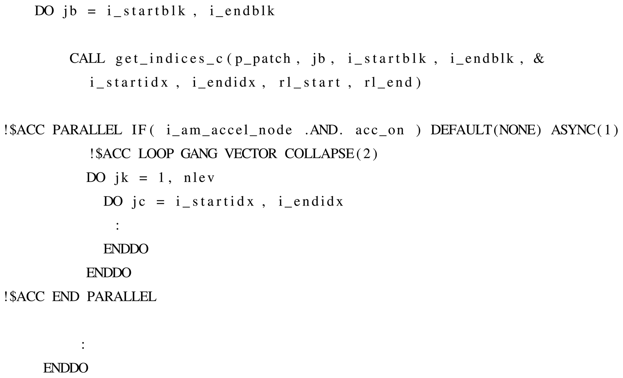
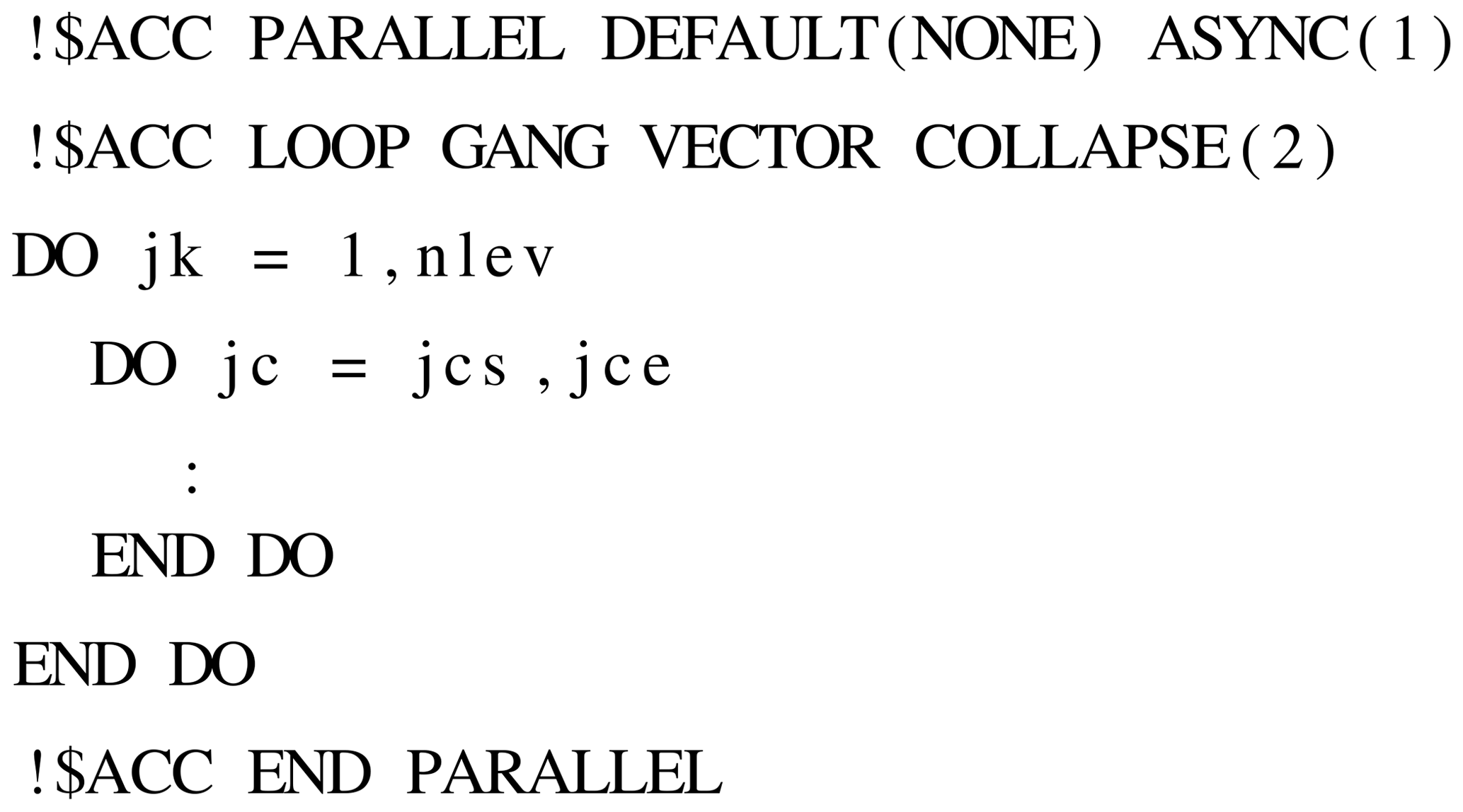
However, this approach turned out to be a considerable limitation: in the physical parameterizations, the loop over all blocks is many subroutine levels above the loops over the block and the levels. Although it is in theory possible to construct an OpenACC parallel region with a complex and deep subroutine call tree, in practice it proves not to be a viable approach with the available OpenACC compilers (PGI and Cray). In order to avoid a complex programming technique, it was decided to refactor the dynamical core to parallelize only over the two inner dimensions, nproma and nlev, when possible; see Listing 1. With this approach the optimal nproma is chosen as large as possible, i.e., having effectively one block per MPI subdomain and thus a single iteration in the jb loop in Listing 1.
Generally kernels are denoted with the ACC PARALLEL directive, which allows the user to be more prescriptive than the higher-level descriptive ACC KERNELS directive, which is used in ICON only for operations using Fortran array syntax. Usage of KERNELS for more complicated tasks tended to reduce performance.
There are code differences between CPU and GPU in the non-hydrostatic solver. On the accelerator it is advantageous to use scalars within loops, while for the CPU, frequently two-dimensional arrays perform better; see Listing 2.
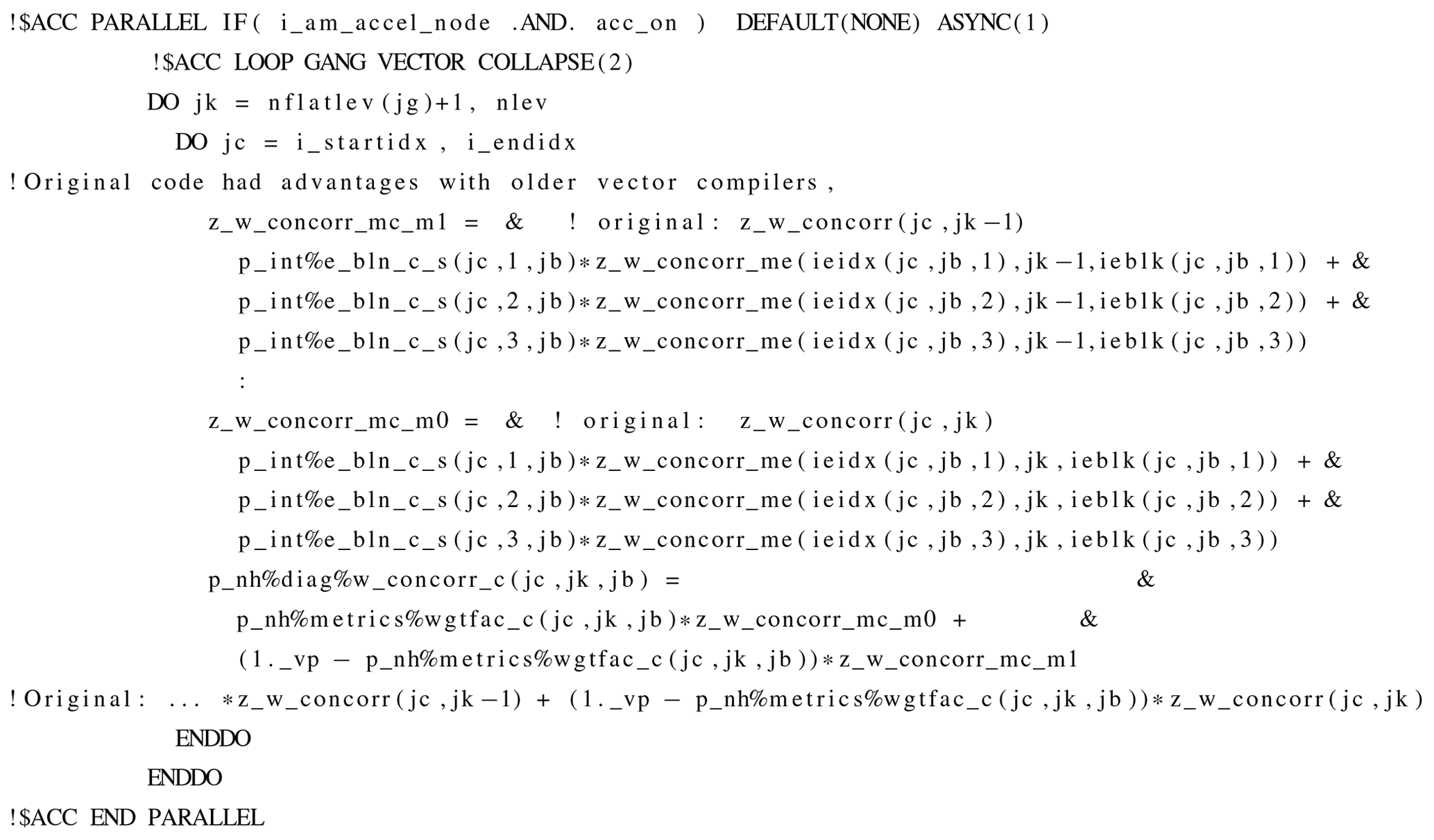
Listing 2Register variables outperform arrays on GPU. One of roughly 10 code divergences in the dynamical core.
After extensive refactoring and optimizations, such as asynchronous kernel execution and strategically placed ACC WAIT directives, the resulting dycore version performed at least as well on GPUs as the original GPU version with triple-nested parallelism, with the former operating with 𝚗𝚋𝚕𝚘𝚌𝚔𝚜=1 or a very small integer and thus the largest possible nproma. See Sect. 6 for complete performance comparisons, in particular between CPU and GPU.
4.3.2 Tracer transport
There are several different variants of horizontal and vertical advection, depending on whether the scheme is Eulerian or semi-Lagrangian, what sort of reconstructions (second- or third-order), and which type of time stepping is employed. All of these variants ultimately can be considered stencil operations on a limited number of neighboring cells, i.e., physical quantities defined in cell centers, vertices, or edges. As such, the structure of the corresponding kernels is usually similar to Listing 1.
In several parts of the code-specific optimization, so-called “index lists” as shown in Listing 3 are employed for better performance on CPUs, in particular for vector machines. The advantage of an index list is that the subsequent calculation can be limited only to the points which fulfill a certain criterion, which is generally quite rare, meaning the list is sparse and thus quite small. In addition, such an implementation avoids the use of “if” statements, which makes it easier for the compiler to auto-vectorize this code section. For the GPU parallelization, such index list implementation unfortunately has a negative impact on performance as the list creation is a sequential operation.

Listing 3Index lists used in vertical flux calculation with reconstruction by the piece-wise parabolic method.
On an accelerator, numerous execution threads will be competing to increment counter_ji and insert indices into i_indlist, i_levlist. We overcame this by using OpenACC atomics or parallel algorithms based on exclusive scan techniques. However, in some cases the proper GPU algorithm is to operate over the full loop. The GPU executes both code paths of the IF statement, only to throw the results of one path away. The algorithm for vflux_ppm4gpu is functionally equivalent (Listing 4).

Some horizontal advection schemes and their flux limiters require halo exchanges in order to make all points in the stencil available on a given process. The communication routines are described in Sect. 4.3.5.
4.3.3 Horizontal diffusion
The dynamical core contains several variants of horizontal diffusion. The default approach is a more physically motivated second-order Smagorinsky diffusion of velocity and potential temperature combined with a fourth-order background diffusion of velocity, using a different discretization for velocity that is formally second-order accurate on equilateral triangles.
Most of the horizontal diffusion contains kernels in the style of Listing 1, but again there are index lists for the normal CPU calculation. Listing 5 illustrates how the index lists are avoided at the cost of a temporary 3-D array.
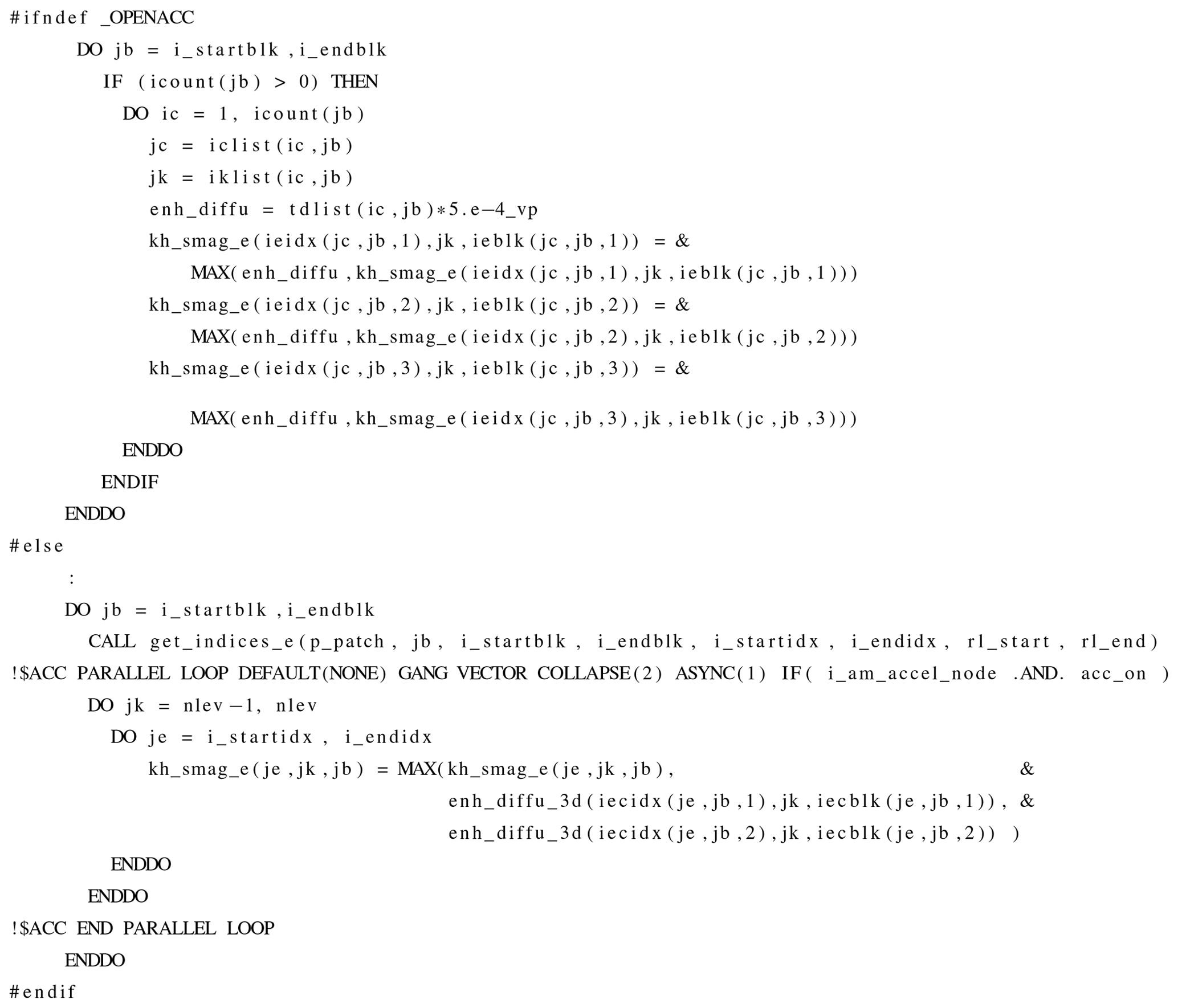
Listing 5The OpenACC version uses a temporary 3D array enh_diffu_3d defined in cell centers and a revised MAX statement on the edge grid to avoid the construction of iclist/iklist from the previous loop.
4.3.4 Dynamical core operators
The dynamical core also calls horizontal operators such as averaged divergence or cell-to-vertex interpolation. These operators, along with numerous related stencil operations required in other parts of the model, were also ported with OpenACC. These almost always adhere to the style of Listing 1 and are thus straightforward to port to OpenACC.
4.3.5 Dynamical core infrastructure
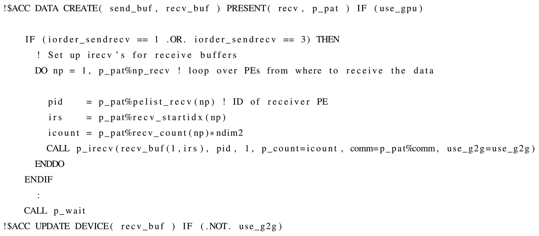
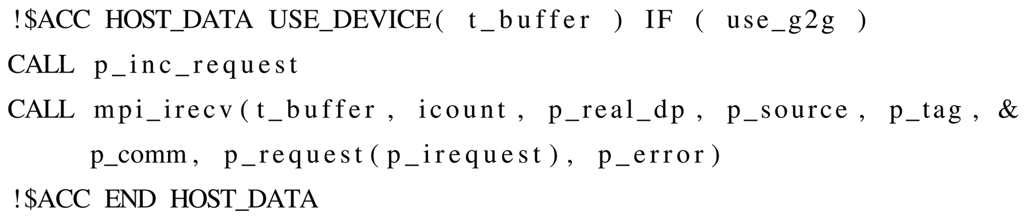
Essentially all of the halo exchanges occur in the dynamical core, the horizontal flux calculation of advection, or in the dynamics–physics interface. During the exchange, the lateral boundary cells of a vertical prism residing on a given process are written into the lateral halo cells of vertical prisms residing on its neighboring processes. Since these halo exchanges are performed within the time loop, the halo regions are in device memory. Two mechanisms are available to perform the exchange:
-
Update the prism surface on the CPU, post the corresponding MPI_Isend and Irecv with a temporary (host) buffer, and after the subsequent MPI_WAIT operation, update receive buffer on the device, and copy the buffer to the halo region solely on the device.
-
Pass GPU pointers to the same Isend and Irecv routines in a GPU-aware MPI implementation. The final copy to the halo region is again performed on the device.
These two mechanisms illustrated in Listings 6 and 7 are easily woven together with logicals in the corresponding OpenACC IF clauses.
4.4 Physical parameterizations
The provision of the physical forcing for the time integration is organized in four levels outlined in Listing 8. The first level, which is the dynamics–physics interface, transforms the provisional variable state X(t) that results from dynamics and transport (Fig. 2) to the physics variable state Y that is the input for the physical parameterizations (Fig. 3). And on return from the physics, the collected total tendencies from physics in Y variables are converted to tendencies in the X variables, followed by the computation of the new state X(t+dt). These tasks involve loops over blocks, levels, and grid points as in dynamics. Their parallelization on the GPU therefore follows the pattern used in the dynamics codes; see Listing 1.
At the second level, the physics main routine calls the physical parameterizations of the Sapphire configuration in the sequence shown in Fig. 3 by use of a generic subroutine. This routine contains the block loop from which the specified parameterization interface routine is called for each single data block. Thus the computation below this level concerns only the nproma dimension over cells and the nlev dimension over levels and in some cases extra dimensions, for instance, for tracers or surface tiles. Note that the second-level interface and the generic subroutine do not compute any fields and therefore do not use the GPU and are free of OpenACC directives.
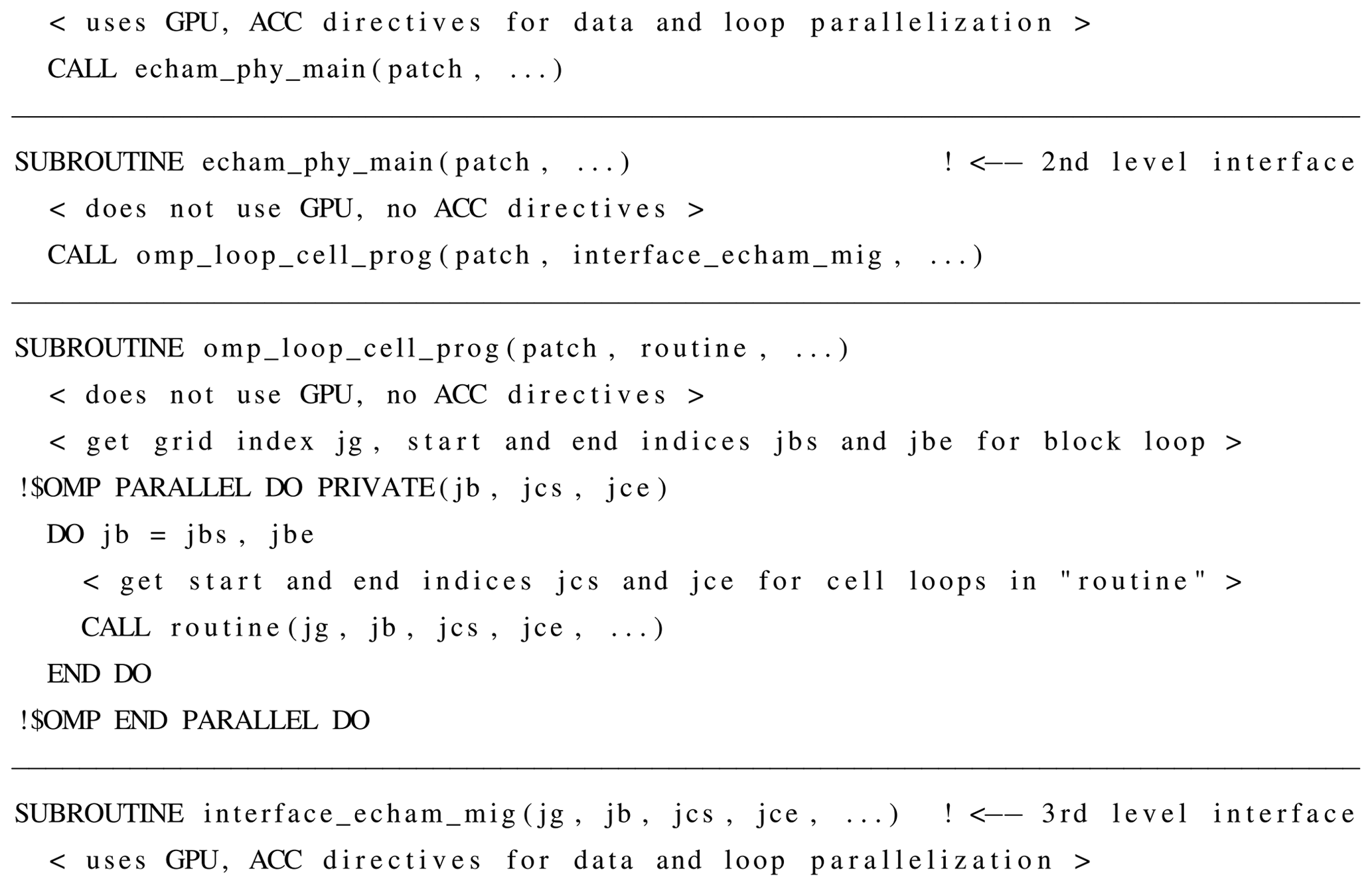
Listing 8Lines from the first- to third-level interfaces and the generic routine with the block loop used in the second-level interface for calling the third-level interface routines for specific parameterizations, here for the example of graupel cloud microphysics (mig).
The third level consists of the interfaces to the specific parameterizations. These interfaces provide access to the global memory for the parameterizations by USE access to memory modules. The equivalent variables in GPU memory, which have been created before and updated where necessary, are now declared individually as present, as, for instance, the three-dimensional atmospheric temperature ta and the four-dimensional array qtrc for tracer mass fractions in $ACC DATA PRESENT(field %ta, field %qtrc). This practice was followed in the code used on Piz Daint. The newer code on JUWELS Booster instead declares the entire variable construct as present instead of its components, like $ACC DATA PRESENT(field). Beside the memory access, these interfaces use the output of the parameterization for computing the provisional physics state for the next parameterization in the sequentially coupled physics and for accumulating the contribution of the parameterization tendencies in the total physics tendencies. These tasks typically require loops over the nproma and nlev dimensions but sometimes also over additional dimensions like tracers. The typical loop structure follows Listing 9.
Listing 9Most common loop structure over levels jk and cells jc in parameterizations and their interfaces.
Particular attention is paid to the bit-wise reproducibility of sums, as for instance for vertical integrals of tracer masses computed in some of these interfaces in loops over the vertical dimension. Here the !$ACC LOOP SEQ directive is employed to fix the order of the summands. This bit-wise reproducibility is important in the model development process because it facilitates the detection of unexpected changes of model results, as further discussed in Sect. 5.
Finally, the fourth level exists in the parameterizations. The parameterizations used here are inherently one-dimensional, as they couple levels by vertical fluxes. This would allow them to be encoded for single columns, but for traditional optimization reasons, these codes include a horizontal loop dimension, which in ICON is the nproma dimension. Therefore, these parameterizations include this additional loop beside those required for the parameterization itself. The presence of these horizontal loops favored the GPU parallelization, which therefore generally follow the pattern in Listing 9. Some parameterization-specific modifications of the GPU parallelization are pointed out in the following sections.
4.4.1 Radiation
As pointed out earlier, the GPU implementation aims at using maximum block sizes, so that all grid points and levels within a computational domain fit into a single block, and hence a single iteration of the block loop suffices. Using large block sizes, however, means also that more memory is required to store the local arrays, which is a challenge, especially on Piz Daint with the small GPU memory capacity. This problem turned out to be most pronounced for the radiation code, owing to the extra spectral dimension. On Piz Daint, this meant that a single block per domain would not have been feasible. This issue was resolved by allowing for a sub-blocking parameter rrtmgp_column_chunk (rcc) in the radiation code, so that the original blocks of size nproma are broken up into smaller data blocks for input and output of the radiation scheme. This radiation block size can be specified as necessary and is typically ca. 5 % to 10 % of nproma when using the smallest possible number of nodes. But, at the largest node counts during strong scaling as shown in the experiments below, nproma can become small enough so that no sub-blocking in the radiation is needed, and rcc is set to the number of grid points in the computational domain.
As explained in Pincus et al. (2019), RTE+RRTMGP comprises a set of user-facing code, written in object-oriented Fortran 2008, which is responsible for flow control and input validation, etc. Computational tasks are performed by computational kernels using assumed-size arrays with C bindings to facilitate language interoperability. For use on GPUs, a separate set of kernels was implemented in Fortran using OpenACC directives, with refactoring to increase parallelism at the cost of increased memory use relative to the original CPU kernels. The Fortran classes also required the addition of OpenACC data directives to avoid unnecessary data flows between CPU and GPU.
RTE+RRTMGP, like ICON, operates on sets of columns whose fastest-varying dimension is set by the user and whose second-fastest varying dimension is the vertical coordinate. Low-level CPU kernels are written as loops over these two dimensions, with higher-level kernels passing results between low-level kernels while looping over the slowest-varying spectral dimension. This approach, illustrated in Listing 10, keeps memory use modest and facilitates the reuse of cached data. Low-level GPU kernels, in contrast, operate on all three dimensions at once. When the calculation is parallelizable in all dimensions, i.e where values at every spatial and spectral location are independent, the parallelization is over all elements at once. Some loops have dependencies in the vertical; for these the GPU kernels are parallelized over the column and spectral point, with the vertical loop performed sequentially within each horizontal and spectral loop (see Listing 11).
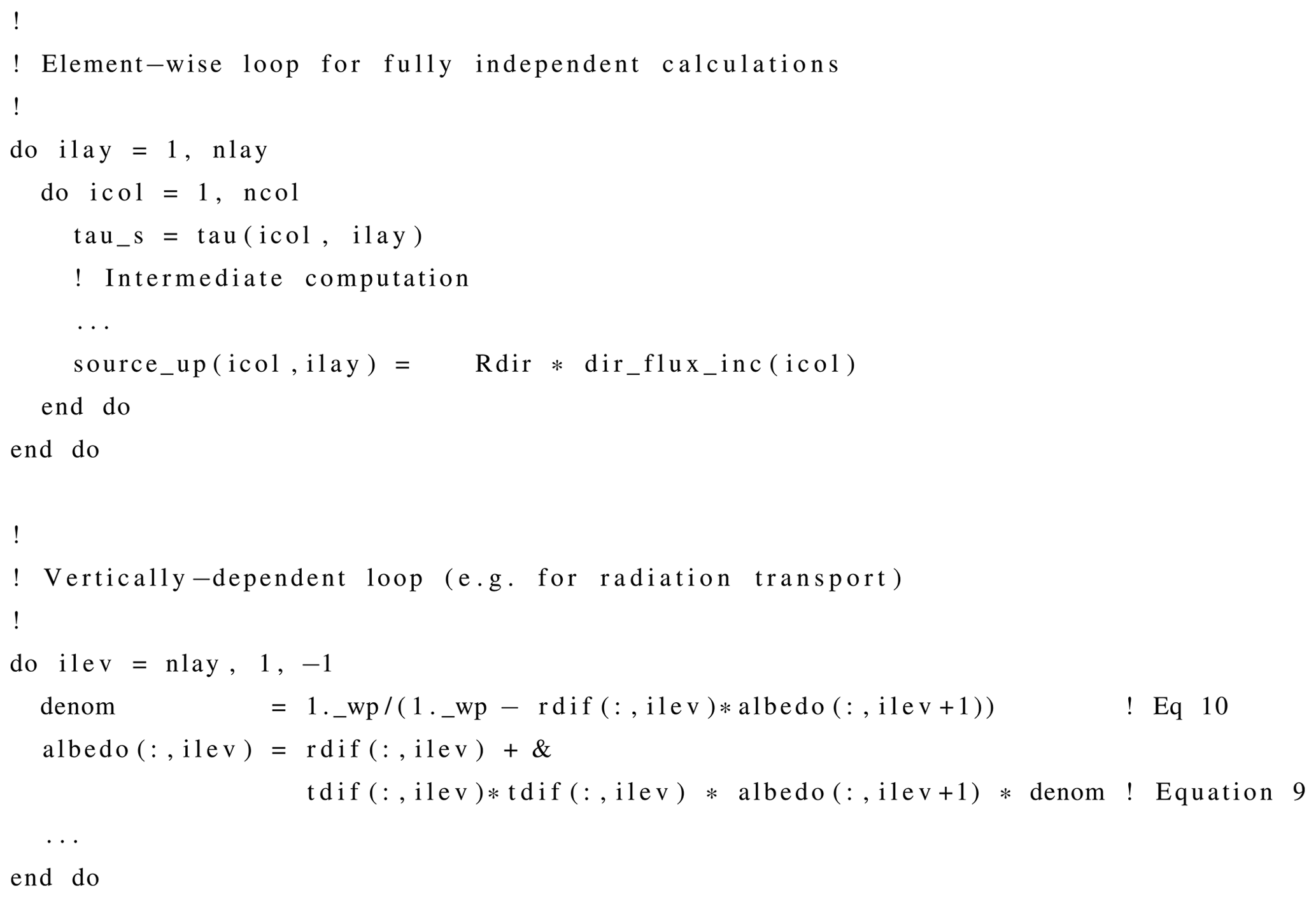
Listing 10Example loop structure for CPU kernels in RTE+RRTMGP. High-level kernels operate on all levels and columns in the block but only one spectral point (g-point) at a time. In this example the loop over g-points is performed at one higher calling level.

Listing 11Example loop structure for GPU kernels in RTE+RRTMGP. For the GPUs, kernels operate on all levels, columns, and spectral points at once, expect where dependencies in the vertical require the vertical loop to be done sequentially.
Most sets of kernels in RTE+RRTMGP now contain two separate implementations organized in distinct directories with identical interfaces and file naming. A few sets of kernels (e.g., those related to summing over spectral points to produce broadband fluxes) were simple enough to support the addition of OpenACC directives into the CPU code.
Though the original plan was to restrict OpenACC directives to the kernels themselves, it became clear that the Fortran class front ends contain enough data management and small pieces of computation that they, too, required OpenACC directives, both to keep all computations on the GPU and to allow for the sharing of data from high-level kernels (for example, to reuse interpolation coefficients for the computation of absorption and scattering coefficients by gases). The classes therefore have been revised such that communication with the CPU is not required if all the data used by the radiation parameterization (temperatures, gas concentrations, hydrometeor sizes, and concentrations, etc.) already exist on the GPU.
4.4.2 Land surface physics
One of the design goals of the new ICON-Land infrastructure has been to make it easy for domain scientists to implement the scientific routines for a specific land model configuration, such as JSBACH. Except for the (lateral) river routing of runoff, all processes in JSBACH operate on each horizontal grid cell independently, either 2-D or 3-D with an additional third dimension such as soil layers, and therefore do not require detailed knowledge of the memory layout or horizontal grid information. To further simplify the implementation, the 2-D routines are formulated as Fortran elemental subroutines or functions, thus abstracting away the field dimensions of variables and loops iterating over the horizontal dimension. As an intermediate layer between the infrastructure and these scientific routines, JSBACH uses interface routines which are responsible for accessing variable pointers from the memory and calling the core (elemental) calculation routines. These interfaces make extensive use of Fortran array notation. Consequently, the implementations of the land process models have no explicit loops over the nproma dimension, in contrast to the atmospheric process models, where the presence of these loops favored the GPU parallelization.
Instead of refactoring large parts of JSBACH to use explicit ACC directives and loops and thus hampering the usability for domain scientists, the CLAW (Clement et al., 2018) source-to-source translator has been used for the GPU port. CLAW consists of a domain-specific language (DSL) and a compiler, allowing it to automate the port to OpenACC with much fewer directives and changes to the model code than are necessary with pure ACC. For example, blocks of statements in the interface routines using array notation can simply be enclosed by !$claw expand parallel and !$claw end expand directives and are then automatically expanded into ACC directives and loops. An example of this mechanism, as used in the JSBACH interface to radiation, is shown in Figs. 8 and 9 of Clement et al. (2019).
The elemental routines discussed above are transformed into ACC code using an additional CLAW feature: the CLAW Single Column Abstraction (SCA) (Clement et al., 2018). The CLAW SCA has been specifically introduced in CLAW to address performance portability for physical parameterizations in weather and climate models which operate on horizontally independent columns. Using the CLAW SCA translator, the only changes necessary in the original Fortran code of JSBACH were to
-
prepend the call to an elemental routine by the CLAW directive
!$claw sca forward, -
insert
!$claw model-dataand!$claw end model-dataaround the declaration of scalar parameters in the elemental routine that need to be expanded and looped over, -
insert a
!$claw scadirective in the beginning of the statement body of the elemental routine.
The CLAW SCA transformation then automatically discards the ELEMENTAL and PURE specifiers from the routine, expands the flagged parameters to the memory layout specified in a configuration file, and inserts ACC directives and loops over the respective dimensions. Examples for the original and transformed code of the JSBACH routine calculating the net surface radiation are shown in Figs. 5 and 6, respectively, of Clement et al. (2019).
More details on the CLAW port of JSBACH including performance measurements for the radiation component of JSBACH can be found in Clement et al. (2019).
4.4.3 Cloud microphysics
Cloud microphysical processes are computed in three sequential steps: (1) saturation adjustment for local condensation or evaporation; (2) the microphysics between the different hydrometeors and the vertical fluxes of rain, snow, and graupel; and (3) again saturation adjustment for local condensation or evaporation. Here the code for the saturation adjustment exists in a CPU and GPU variant, selected by a compiler directive. The CPU code sets up one-dimensional lists of cell and level indices, where the adjustment requires Newton iterations, while the GPU code uses a logical two-dimensional mask with nproma and nlev dimensions for the same purpose. The CPU code then loops over the cells stored in the index lists, while the GPU code employs a two-dimensional loop structure in which computations happen only for the cells selected by the mask. Beside the different means to restrict the computations to the necessary cells, the CPU code is also optimized for vectorizing CPUs, which is the reason that the loop over the list occurs within the condition for ending the Newton iteration cycles, while the GPU code checks this within the parallelized loops. The related code fragments are shown in Listings 12 and 13.
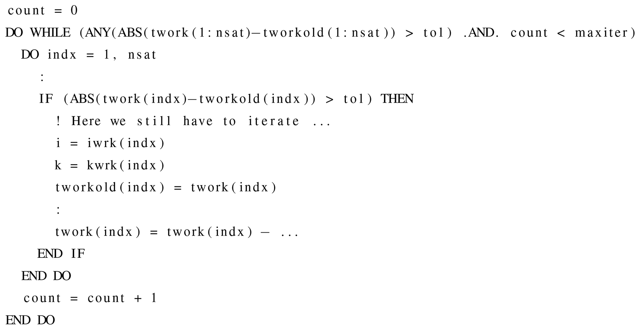
Listing 12Code structure of the Newton iteration for the saturation adjustment on CPU, making use of 1D lists iwrk for the cell index and kwrk for the level index of cells where the adjustment needs to be computed iteratively.

Listing 13Code structure for saturation adjustment on GPU, making use of a 2D mask iwrk for the cell index and kwrk for the level index of cells where the adjustment needs to be computed iteratively.
The ICON development on CPU makes use of test suites comprising simplified test experiments for a variety of model configurations running on a number of compute systems using different compilers and parallelization setups. This includes the AMIP experiment discussed in Giorgetta et al. (2018) but is shortened to four time steps. The test suite for this experiment checks for reproducible results with respect to changes of the blocking length, amount, and kind of parallelization (MPI, OpenMP, or both), as well as checks for differences to stored reference solutions. This test suite was also implemented on Piz Daint, where the experiments have been run by pure CPU binaries as well as GPU-accelerated binaries. Output produced on these different architectures – even if performed with IEEE arithmetic – will always produce slightly different results due to rounding. Therefore, the above-mentioned tests for bit identity cannot be used across different architectures. The problem is made worse by to the chaotic nature of the underlying problem. These initially very small changes, which are on the order of floating point precision, quickly grow across model components and time steps, which makes distinguishing implementation bugs from chaotically grown round-off differences a non-trivial task.
This central question of CPU vs. GPU code consistency was addressed in three ways, (1) the “ptest” mode, (2) the serialization of the model state before and after central components, and (3) tolerance tests of the model output. Details for these methods are given in the following subsections. The first two methods are able to test a small fraction of the code in isolation where chaotic growth of round-off differences is limited to the tested component and thus small. We found that tolerating relative errors up to differences of 10−12 with double-precision floating point numbers (precision roughly at 10−15) did not result in many false positives (a requirement for continuous integration) while still detecting most bugs. Even though most of the code is covered by such component tests, there is no guarantee that passing all these tests leads to correct model output. To ensure this, a third method had to be implemented. This method came to be known as the “tolerance test” because tolerance ranges could not be assumed constant but had to be estimated individually for each variable across all model components and over multiple time steps. It should be emphasized that, while the introduction of directives took only weeks of work, the validation of proper execution with the inevitable round-off differences between CPU and GPU execution took many months.
5.1 Testing with the ptest mode
The preexisting internal ptest mechanism in ICON allows the model to run sequentially on one process and in parallel on the “compute processes” with comparisons of results at synchronization points, such as halo exchanges. This mechanism was extended for GPU execution with the addition of IF statements in kernel directives, so that the GPUs are only active on the compute processes. Listing 1 illustrates all of the above-mentioned ideas. In particular, the global variable i_am_accel_node is .TRUE. on all processes which are to execute on accelerators but .FALSE. on the worker node delegated for sequential execution.
If the ptest mode is activated when a synchronization point is encountered, arrays calculated in a distributed fashion on the MPI compute processes are gathered and compared to the array calculated on the single sequential process. Synchronization points can either be halo exchanges or manually inserted check_patch_array invocations which can compare any arrays in the standard 3-D ICON data layout.
While this method was very handy at the beginning of the effort to port the model to GPUs, especially for the dynamical core of the model, extending it beyond the preexisting mechanism turned out to be cumbersome. At the same time, the Serialbox library offered a very flexible way to achieve the same goal without running the same code on different hardware at the same time.
5.2 Serialization
Besides the ptest technique mentioned, two other approaches were used for the validation of GPU results. First, the full model code was used with test experiments, which typically use low resolution, just a few time steps, and only the component of interest. Examples are AMIP experiments on the R2B4 grid, as used in Giorgetta et al. (2018) but for four time steps only, with or without physics, or with only a single parameterization. This approach has the advantage that the experiments can be compared to other related experiments in the common way, based on output fields as well as the log files in all tests.
The second approach, the “serialization” method, uses such experiments only to store all input and output variables of a model component. Once these reference data are stored, the test binary (usually utilizing GPUs) reads the input data from the file and calls the model component in exactly the same way as the reference binary (usually running exclusively on CPUs). The new output is stored and compared to the previously generated reference data, for instance, to check for identical results or for results within defined tolerance limits due to round-off differences between pure CPU and GPU-accelerated binaries. This serialization mechanism was implemented in ICON for all parameterizations (but not dynamics or transport, which were tested with the technique mentioned in Sect. 5.1), which were ported to GPU, and was primarily used during the process of porting individual components to GPU. The advantage of this method is the fine test granularity that can be achieved by surrounding arbitrary model components with the corresponding calls to the serialization library.
5.3 Tolerance testing
The methods discussed in the last two sections are valuable tools to locate sources of extraordinary model state divergence (usually due to implementation bugs) as well as frequent testing during optimization and GPU code development. However, they do not guarantee the correctness of the model output. This problem is fundamentally different from component testing because chaotic growth of initial round-off differences is not limited to a single component but quickly accumulates across all model components and simulation time steps. This section introduces a method to estimate this perturbation growth and how it is used to accept or reject model state divergence between pure CPU and GPU-accelerated binaries.
The idea is to generate for each relevant test experiment on CPU an ensemble of solutions, which diverge due to tiny perturbations in the initial state. In practice the ensemble is created by perturbing the state variables consisting of the vertical velocity w, normal velocities on cell edges vn, the virtual potential temperature θv, the Exner function Π, and the density ρ by uniformly distributed random numbers in the interval [, ]. The resulting ensemble, which consist of the unperturbed and nine perturbed simulations, is used to define for each time step of the test the tolerance limits for all output variables. In practice, we do not compute the tolerance limit for each grid point but define a single value for each variable and time step by applying different statistics across the horizontal dimension and selecting the largest value for each statistic across the vertical dimension. The test is currently implemented using minimum, maximum, and mean statistics in the horizontal. This approach has proved to be effective to discard outliers. Applying the same procedure to the model output from the GPU-accelerated binary allows the test results to be compared with the pure CPU reference under the limits set by the perturbed CPU ensemble. This method proved effective in highlighting divergences in the development of the GPU version of the ICON code over a small number of time steps.
Once the GPU port of all components needed for the planned QUBICC experiments was completed, practical testing was started with the first full experiment shortened to 2 simulation hours – a computational interval that proved to be sufficient to provide robust performance results. For the technical setup, it was found that a minimum of ca. 960 GPU nodes of Piz Daint was necessary for the memory of a QUBICC experiment. Because performance was affected when getting close to 960 nodes, a setup of 1024 nodes was chosen for the model integration. This number 1024=210 also has the advantage that it more easily facilitates estimates of scalings for factor of 2 changes in node counts. Similarly, a minimal number of 128 compute nodes was determined for a QUBICC experiment on JUWELS Booster and Levante.
An additional small number of nodes was allocated for the asynchronous parallel output scheme. The number is chosen such that the output written hourly on Piz Daint and 2-hourly on JUWELS Booster and Levante is faster than the integration over these output intervals. As a result, the execution time of the time loop of the simulation is not affected by writing output. Only does the writing output at the end of the time loop add additional time.
These setups were used for the science experiments including the experiment discussed in Sect. 6.1 as well as starting points for the benchmarking experiments.
6.1 Benchmarking experiments
The test experiment for benchmarking consists of precisely the configuration of dynamics, transport, and physics as for the intended QUBICC experiments. Only the horizontal grid size, the number of nodes, and parameters to optimize parallelization were adjusted as needed for the benchmark tests. The length of the benchmark test is 180 time steps corresponding to 2 h simulated time, using the same 40 s time step in all tests. For all benchmark tests, the time to solution has been measured by internal timers of the model. This provides the data for the discussion of the speedup, time to solution and scaling in Sects. 6.3 to 6.5. These data are available in the related data repository (Giorgetta, 2022).
Three different grid sizes are used for benchmarking. First, for single-node testing on Piz Daint (Sect. 6.3) the R2B4 grid is used because this grid is 1024 times smaller than the R2B9 grid used for experiments running on 1024 Piz Daint nodes. Second, for the strong scaling analysis, the R2B7 grid is used, which is 16 times smaller than the R2B9 grid. Accordingly, the minimal number of nodes used for the strong scaling tests is 16 times smaller than for the R2B9 setup used in experiments, so that this smallest setup is again comparable in memory consumption to the R2B9 setup for the experiments and further so that at least four node doubling steps are possible within the limits of the computer allocations. The actual ranges of compute nodes ncn used for the strong scaling tests for the R2B7 grid on the three computers can be seen in Table 3. Third, for the weak scaling analysis, the R2B9 grid is used, so that it can be compared with the R2B7 tests with 16 times smaller number of grid points and nodes.
The allocations on JUWELS Booster and Levante also allowed us to run benchmark tests for the R2B9 grid on larger node numbers so that the strong and weak scaling could also be analyzed for higher node numbers, as tabulated in Table 3.
Among the three grids used here, only the benchmark test on the original QUBICC grid (R2B9) has a physically meaningful configuration, while benchmark tests with smaller grid sizes are not configured for meaningful experiments. Timings reported below for benchmark tests on smaller grid sizes therefore should not be interpreted as timings for ICON experiments configured for such reduced resolutions, e.g., through the introduction of additional processes or changes in time steps.
Two measures of scaling are introduced. Strong scaling Ss measures how much the time to solution, Tf, is increased for a fixed configuration with 2ncn computing nodes compared to one-half of the time to solution with ncn nodes. Weak scaling Sw measures how much Tf increases for a 2-fold increase in the horizontal grid size (with ngp grid points) balanced by a 2-fold increase in the node count, ncn. These are calculated as
respectively. Because global grids can more readily be configured with grid resolution changing in factors of 2 and consequently ngp changing in multiples of 4, and to minimize the noise for the weak scaling, Sw is estimated through experiments with a 4-fold increase in resolution and 16-fold increases in the computational mesh and node count. An ideal scaling would result in , while Ss<0.5 would indicate a detrimental effect of adding computational resources.
Values of Tf needed in calculating Ss and Sw are provided by the simulation log files. These time measurements, which are part of the model infrastructure, are taken for the integration within the time loop that includes the computations for all processes (dynamics, transport, radiation, cloud microphysics, vertical diffusion, and land processes), as well as other operations required to combine the results from these components, to communicate between the domains of the parallelizations and to send data to the output processes, etc. But for benchmarking, we are mostly interested in the performance of the time loop integration and the above-mentioned processes. The benchmarking should show that the GPU port provides a substantial speedup on GPU compared to CPU, and it should characterize the strong and weak scaling behavior of the ICON model on the compute systems available in this study.

Two model versions have been used in the benchmarking, as listed in Table 2. Version (1) resulted from the GPU porting on Piz Daint and version (2) from the further developments made when porting to JUWELS Booster. This latter version was also used on Levante. The codes of both model versions are available in the related data repository (Giorgetta, 2022).
6.2 Optimization parameters
The computational performance of benchmark experiments can be optimized by the choice of the blocking length nproma, the radiation sub-blocking length rcc, and the communication method. As discussed already in Sect. 4.1, the most important point for execution on GPU is to have all data in a single block on each MPI domain, thus including the grid points for which computations are needed (Table 3, column ngpp) as well as the halo points needed as input for horizontal operations in dynamics and transport. At the same time, the GPU memory must be sufficient to store the local data given the (large) block size.
For Piz Daint, the 1024-node setup for the R2B9 grid has 20 480 horizontal grid points per domain and a nproma value of ca. 21 000. The single-node benchmarking uses the R2B4 grid with nproma = ngpp=20 480 because no halo is needed. Strong scaling tests are based on the R2B7 grid using 64 to 1024 nodes. Thus the initial 64 node setup uses practically the same amount of memory per node as the small single-node test, while the largest setup has a block size ca. 16 times smaller. The weak scaling tests consist of the same R2B7 setup on 64 nodes used for strong scaling and the 16 times larger R2B9 setup on 1024 nodes, which therefore have comparable block sizes of ca. 21 000.
A second performance parameter consists in the size of the sub-blocking used for radiation, rcc, which was introduced to reduce the memory requirement of the radiation and thus to allow for the usage of single blocks for all other components of the model. For setups on Piz Daint with nproma close to 21 000, tests showed that the maximum rcc is 800 (Table 3), thus splitting a data block into 26 sub-blocks for the radiation calculation (). In the strong scaling series, the increasing number of nodes reduces the grid size per node and nproma accordingly, which allows rcc to be increased. Only for 512 nodes did it show that having rcc =1280, which amounts to two sub-blocks of equal size, was more efficient to compute the radiation than having a higher rcc, which triggers two radiation calls with quite unequal sub-block sizes as, for instance, 2000 and 560. Finally, for 1024 nodes, rcc =1280 covers all computational cells so that a single radiation call is sufficient; i.e., no sub-blocking takes place.
Further optimizations can be exploited in the communication. Choosing direct GPU-to-GPU communication instead of CPU-to-CPU communication (see Sect. 4.3.5) results in a speedup of ca. 10 % on Piz Daint. Unfortunately the GPU-to-GPU communication on Piz Daint caused random crashes seemingly related to the MPICH implementation, and therefore all scaling tests and experiments on Piz Daint use the slower CPU communication. On JUWELS Booster, no such problems were encountered, so that the GPU-to-GPU communication is used in all experiments.
On JUWELS Booster, more GPU memory is available compared to Piz Daint (160 GB vs. 16 GB per node). This allows for scaling tests with the same R2B7 and R2B9 grids on a minimum of 8 and 128 nodes, respectively, with a blocking length nproma close to 42 000 and a sub-blocking length rcc starting at 5120 or eight sub-blocks of equal size. This larger sub-blocking length is possible not only because of the larger GPU memory, but also because the newer ICON code that is used on JUWELS Booster has only half of the g-points of the gas optics in the radiation, 240 instead of 480, which reduces the memory for local arrays in radiation accordingly. On JUWELS Booster the strong scaling tests extend from 8 to 256 nodes, thus from 32 to 1024 GPUs. On 64 and more nodes, nproma is small enough to set rcc to the full number of computational grid points in the domain, which allows the radiation scheme to be computed without sub-blocking. Further, it should be pointed out that the reduction of the number of g-points constitutes a major computational optimization by itself, as this reduces the computing costs of this process by a factor 2 without physically significant effects on the overall results of the simulations.
On Levante, where no GPUs are used and the CPUs have a comparatively large memory, the best nproma is 32 for all grids and number of nodes, and no sub-blocking is necessary for the radiation; i.e., rcc is also 32 for all cases. An additional optimization concerns the parallelization between MPI processes and OpenMP threads. In all tests on Levante, we use two CPUs/node × 16 processes/CPU × four threads/process = 128 threads/node.
Table 3Time to solution, Tf; percent of time spent on dynamical solver (Dyn); strong and weak scaling, Ss and Sw respectively; and temporal compression, τ, for experiments on Piz Daint, JUWELS Booster, and Levante with code version (Code) from Table 2, grid name, number of grid points, ngp, number of computing nodes, ncn, number of grid points per MPI process, ngpp, and optimization parameters, nproma and 𝚛𝚌𝚌. Scaling values shown in bold are used in the extrapolation for a 1 SYPD simulation at ca. 1 km resolution; see Sect. 6.5.1. The temporal compression is only shown for the R2B9 setup, to which the chosen time step (40 s) corresponds.

6.3 Single-node CPU-to-GPU speedup on Piz Daint
On Piz Daint the achievable speedup of a small R2B4 model setup on a single GPU versus a single CPU was an important metric. Single-node tests give a clear indication of the performance speedup achievable on GPUs vs. CPUs without side effects from parallelization between nodes. Only a speedup clearly larger than 2 would be an improvement for a node hosting one CPU and one GPU versus a node with two CPUs. To achieve this goal, the speedup must be favorable, especially for the model components which dominate the time to solution of the integration.
Figure 4 therefore shows in panel (a) the relative costs of the model components on the GPU as percentage of the time to solution of the integration in the time loop and in panel (b) the CPU-to-GPU speedup for the integration and the model components. Concerning the relative costs, it is clear that dynamics and radiation are the dominating components, each taking between 30 % and 40 %. All other components consume less than 10 % of the integration time. Also the CPU-to-GPU speedup varies between the components. The highest value is achieved by radiation, 7.4, and the lowest by the land scheme, 2.9. All together, the speedup of the full integration is 6.4, as a result of the high scaling of the most expensive components and the very low costs of the components with a lower speedup.
The high speedup of radiation is attributed to the higher computational intensity and more time invested in optimizations as compared to other, less costly components. The land physics stands out for its poor performance, which is attributed to the very small GPU kernels, so that the launch time is often comparable to the compute time. But for the same reason (small computational cost), this has little effect on the speedup of the full model. The 6.4-fold speedup of the code of the whole integration is considered satisfactory, given that the ICON model is bandwidth-limited, and the GPU bandwidth : CPU bandwidth ratio on Piz Daint is of approximately the same order.

Figure 4For a small setup with 20 480 grid points and 191 levels integrated over 180 time steps: (a) time to solution on GPU of the model components as percentage of the time for the “integrate” timer that measures the whole time loop and (b) the CPU-to-GPU speedup for the whole time loop as well as the model components.
6.4 Scaling
On each compute system, the R2B7 and R2B9 setups are run for successive doublings of ncn, starting from the minimum value of ncn (ncn,min) that satisfies the memory requirements of the model and proceeding to the largest ncn for which we could obtain an allocation. Blocking sizes are optimized for each value of ncn. The smaller memory requirements of R2B7 allow it to be run over a much larger range of ncn. In each case, the full time to solution Tf measured for the model integration is provided in Table 3. (The time to solution per grid column and time step can be calculated straightforwardly from these data as .) The strong and weak scaling parameters are then calculated from Tf and Eq. (1). First we discuss the R2B7 benchmarks made for the strong scaling analysis, followed by the weak scaling analysis based on R2B7 and R2B9 benchmarks.
6.4.1 Time to solution and strong scaling of the model integration
The full time to solution Tf and the cumulative strong scaling Ss,cum of the model integration on the R2B7 grid, as measured by the “integrate” timer, are displayed in Fig. 5. The time to solution for the smallest setups clearly shows that the GPU machines allow a solution to be reached more quickly than the CPU machine, when small node numbers are used. And as expected, the more modern JUWELS Booster machine is faster than the older Piz Daint machine. The benefit of repeatedly doubling the GPU node count decreases, as visible in the flattening of the time-to-solution series for Piz Daint and JUWELS Booster. Generally only two doubling steps are possible if Ss,cum should be higher than 0.5. For JUWELS Booster, where the allocation allowed for a fifth doubling step, the time to solution of the last step, at 256 nodes, is actually higher than for 128 nodes. For Levante, the time to solution essentially halves for each doubling of nodes, except for a small degradation building up towards the highest node counts. This makes it already clear that the strong scaling of this experiment differs substantially between the GPU machines Piz Daint and JUWELS Booster and the CPU machine Levante.
Indeed the scaling panel shows that the GPU machines have a cumulative strong scaling Ss,cum that decays rather quickly, almost linearly with the number of node doubling steps. Correspondingly, also the single step strong scaling Ss decreases with increasing node counts, as can be seen in Table 3 for Piz Daint and JUWELS Booster. For Levante we find, however, that Ss,cum even slightly increases in the first two doubling steps, before showing a weak degradation, so that Ss,cum exceeds 0.6, even at the highest tested parallelization on 512 nodes with a 64 times increased node count, where only 80 grid columns are left per MPI process. This results from favorable Ss values even at high node counts, with Ss staying above 0.9 up to 256 nodes; see Table 3.
6.4.2 Time to solution of components
The measurement of Tf of the model components in the strong scaling benchmarks allows for quantification of the relative costs of the main components. Typically the most time-consuming components not only dominate the total time, but also often determine the scaling behavior of the model. Thus knowing the relative costs and the scaling of the components contributes to understanding the behavior of the full model and can give guidance for future improvements. For these purposes, Tf from the dynamical core, tracer transport, radiative transfer, turbulent mixing processes, cloud microphysics, and land processes is displayed in the left column of Fig. 6 for all three compute systems. Among these components, the dynamics generally dominates, taking about 40 % of the compute time on the GPU systems and closer to 50 % of the time on Levante (see Table 3 for precise percentages). The fraction of the compute time spent on the dynamics decreases for high node counts as the model stops scaling. On Piz Daint, radiation is the second most computationally expensive component, while on JUWELS Booster transport is substantially more costly. This difference results from the changed setup of the radiation code used on JUWELS Booster and Levante, which includes (1) the reduction of g-points from 480 to 240 and (2) avoiding the extra computation of clear-sky fluxes. In the smallest R2B7 setup on JUWELS Booster, the first step reduces the radiation time by 43 %, and both steps together yield a reduction of 60 %. On Levante, where also the faster radiation is used, the compute time spent in transport and radiation is almost equal.
The ranking of the less costly processes partly depends on the scaling of the components, which makes the radiation scheme relatively cheaper and the land processes relatively more expensive for higher number of nodes. On the GPU machines Piz Daint and JUWELS Booster, the least amount of time is spent for cloud microphysics for all numbers of nodes, while on the CPU machine Levante, the same is true for the land processes. This points again at the poor CPU-to-GPU speedup of the land scheme and in addition also at a poor strong scaling. However, the total cost of the microphysical complexity is much larger, as in the absence of microphysics there would be no need for tracer transport, which is computed here for six tracers, and the vertical diffusion would be computed only for temperature and wind.
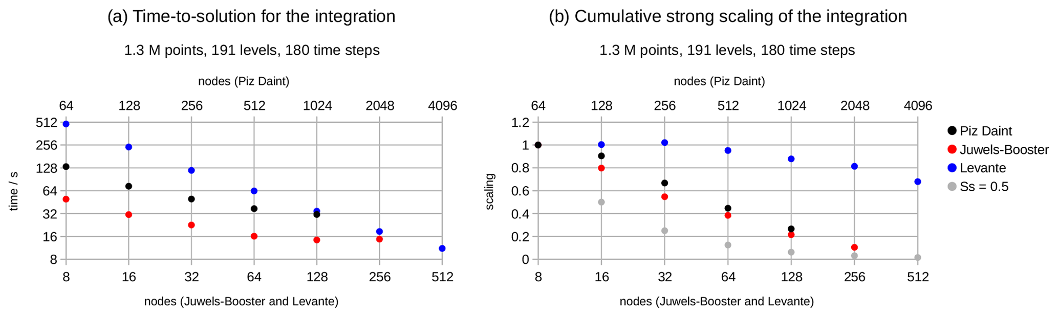
Figure 5Time to solution (a) and cumulative strong scaling Ss,cum (b) from the model integration on Piz Daint (black), JUWELS Booster (red), and Levante (blue). The scaling panel additionally shows in grey Ss,cum for Ss=0.5 for a constant time to solution.

Figure 6Time to solution (a, c, e) and cumulative strong scaling Ss,cum (b, d, f) for Piz Daint (a, b), JUWELS Booster (c, d), and Levante (e, f). The time used and the cumulative strong scaling are shown for the model components: in blue the resolved processes dynamics and transport; in red the atmospheric parameterizations for radiation, vertical diffusion, and cloud microphysics, and in brown the land physics. The scaling panels additionally shows in grey Ss,cum for Ss=0.5 for a constant time to solution.
6.4.3 Strong scaling of components
The cumulative strong scaling Ss,cum of the components is shown in the right column of Fig. 6. Most components show similar scaling behavior to the model as a whole (Fig. 5b), with some noteworthy exceptions. On the GPU machines Piz Daint and JUWELS Booster, the important exceptions to this rule are the land and radiation. Land shows very poor strong scaling, quickly approaching the cumulative strong scaling for Ss=0.5, shown by grey symbols, where the time to solution is constant for all node numbers. Radiation, however, achieves a scaling better than 1 on Piz Daint and remains close to 1 on JUWELS Booster in the first and second doubling of nodes, only starting to decay for larger increases in ncn.
The strong scaling on GPUs depends sensitively on the ability to maintain sufficient work for each node as the node count is increased. In the case of land, which is computationally inexpensive and spatially sparse, this is not possible. For radiation, the workload can be increased through the optimization of the sub-blocking parameter, 𝚛𝚌𝚌. On Piz Daint this is possible up to reaching the case of no sub-blocking in the last step only, on 1024 nodes; see Table 3. On JUWELS Booster the initial sub-blocking size is substantially larger from the beginning, owing to the larger available memory, and thus the largest workload is already reached on 32 nodes. From this step onward, no sub-blocking is needed and the work load decays with the decreasing number of grid points on the processor.
Not critical but noteworthy is the scaling of transport. Generally, the scaling of transport resembles that of dynamics, as both schemes have horizontal dependencies. But for the first node doubling on Piz Daint and the second node doubling on Levante, transport shows a remarkably higher strong scaling than dynamics. Further, on Levante the cumulative strong scaling of the vertical diffusion takes a value of 1 from 8 to 64 nodes and increases for higher node counts up to 1.2 for 512 nodes. The reasons for these behaviors have not been investigated.
6.4.4 Weak scaling
The weak scaling Sw derived from pairs of R2B7 and R2B9 benchmarks with a factor 16 in node count and grid points is shown in Table 3. Generally we found a very good weak scaling, whether on GPUs or on CPUs. For JUWELS Booster and Levante, where Sw was evaluated for more than one pair of R2B7 and R2B9 experiments, Sw remains higher than 0.97 for all cases.
6.4.5 Scaling evaluation
For the practical employment of the ICON-A model, here in the QUBICC configuration, the scaling results have the following consequences. (1) On GPU machines the possibility to speed up the turnover rate along the strong scaling line is rather limited. Starting from the smallest setup, only a doubling or quadrupling of the number of compute nodes would be reasonable. (2) On the CPU machine, the high strong scaling allows the turnover to be increased with little scaling loss, as long as the number of grid columns stays roughly above 100. (3) The excellent weak scaling would allow the horizontal resolution to be increased to the largest grid fitting in the memory of these systems. Thus a resolution of 2.5 km (R2B10 grid) would be possible on Piz Daint and JUWELS Booster. And Levante is large enough for a resolution of 1.25 km (R2B11 grid).
6.5 Outlook for 1 simulated year per day at 1 km resolution on a global grid
6.5.1 Temporal compression of benchmarks
The temporal compression, τ, of a model setup on an available compute systems is important for determining what kind of scientific questions the model may be used for. Here it is measured as a unit-less parameter, of simulated days per day (SDPD), and only calculated for the R2B9 benchmark simulations for which the correct physical configuration and time step are used. Achieving a full simulated year per day (1 SYPD = 365.25 SDPD) for kilometer-scale configurations is a target for centennial-scale climate simulations and still a major challenge.
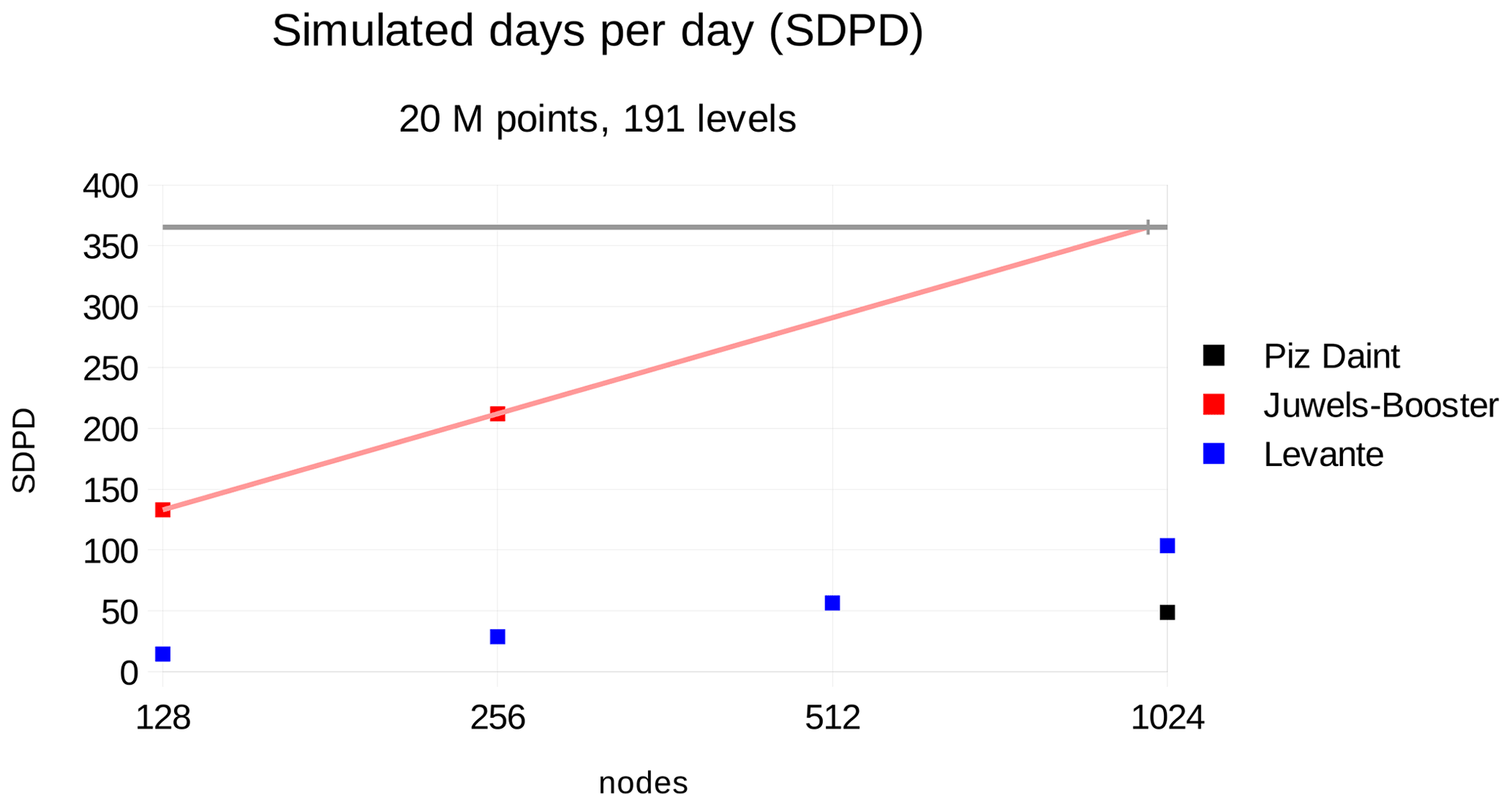
Figure 7Simulated days per day R2B9 (20 M points) based on the integrate timer on Piz Daint, JUWELS Booster, and Levante. The black horizontal line indicates 1 simulated year per day. The thin red line is a linear fit in log(nodes) for the JUWELS Booster simulations. The vertical markers on the 1 sim. year per day line indicate the estimated number of nodes for the integration of a full year on JUWELS Booster: 984 nodes.
The temporal compression of the R2B9 benchmarks is shown in Fig. 7 and also tabulated in Table 3. On Piz Daint the R2B9 experiment on 1024 nodes achieves a temporal compression of 48 SDPD. Considering the poor strong scaling, 1 SYPD is well beyond reach. On Levante, where the experiment has been run on 128, 256, 512, and 1024 nodes, the turnover grows from 14.7 to 103.7 SDPD. Hence, using the entire machine gets closer but still falls about 25 % short of 1 SYPD. On JUWELS Booster a turnover of 133 and 212 SDPD was achieved on 128 and 256 nodes respectively. The linear extrapolation in log(ncn), shown as a thin red line in Fig. 7, indicates that ca. 984 nodes could return about 1 SYPD. Thus the entire JUWELS Booster system that has 936 nodes would get close to 1 SYPD with the model setup for QUBICC experiments.
6.5.2 Computational demands for 1 SYPD
Based on the results above, we extrapolate to assess the computation requirements for a global simulation using an R2B11 (1.25 km) mesh with a temporal compression of 1 SYPD. We base our estimates on reference calculations using the QUBICC configuration, anticipating that its increased number of vertical levels would be commensurate with the target system. Further, we assume that a time step 4 times smaller is stable on the R2B11 grid.
Our calculations of weak scaling allow us in a first step to estimate the performance of an R2B11 system using a 16-fold enlarged setup on an enlarged version of one of the reference compute systems (Ref → 16×Ref). Then we use the strong scaling factor for the reference system to estimate the increase in the temporal compression for a 4-fold larger setup (16×Ref → 64× Ref). For this strong scaling calculation, we use the two Ss values starting from the R2B7 setup with the same number of grid points per node as used in the R2B9 setup enlarged 16-fold in the weak scaling step. Sw and Ss values used for the extrapolation are shown in bold in Table 3. The parameter γ1, measures the gap, i.e., the additional factor of temporal compression required to reach 1 SYPD (Table 4); alternatively it can be understood as the number of days required to simulate 1 year for a given configuration.
Table 4ICON R2B11 configurations and their expected turnover. Compute system with processor type, its total number of nodes and the Rmax LINPACK benchmark, and ICON code version, ICON grid, horizontal resolution (Δx), time step, number of nodes, fraction of nodes with respect to the total number of nodes, temporal compression τ (in SDPD), the gap factor, γ1 for 1 simulated year per day, defined as , and the required computational power , where , and given in units of exaflops per second (EFlop s−1) required to simulate 1 year per day of the indicated model on the indicated configuration of the machine, assuming ideal strong scaling for a speedup of γ1. Because we use the LINPACK references for Rmax, the ncn,tot for Levante is not its present node count but the number used in the November 2021 benchmarks.
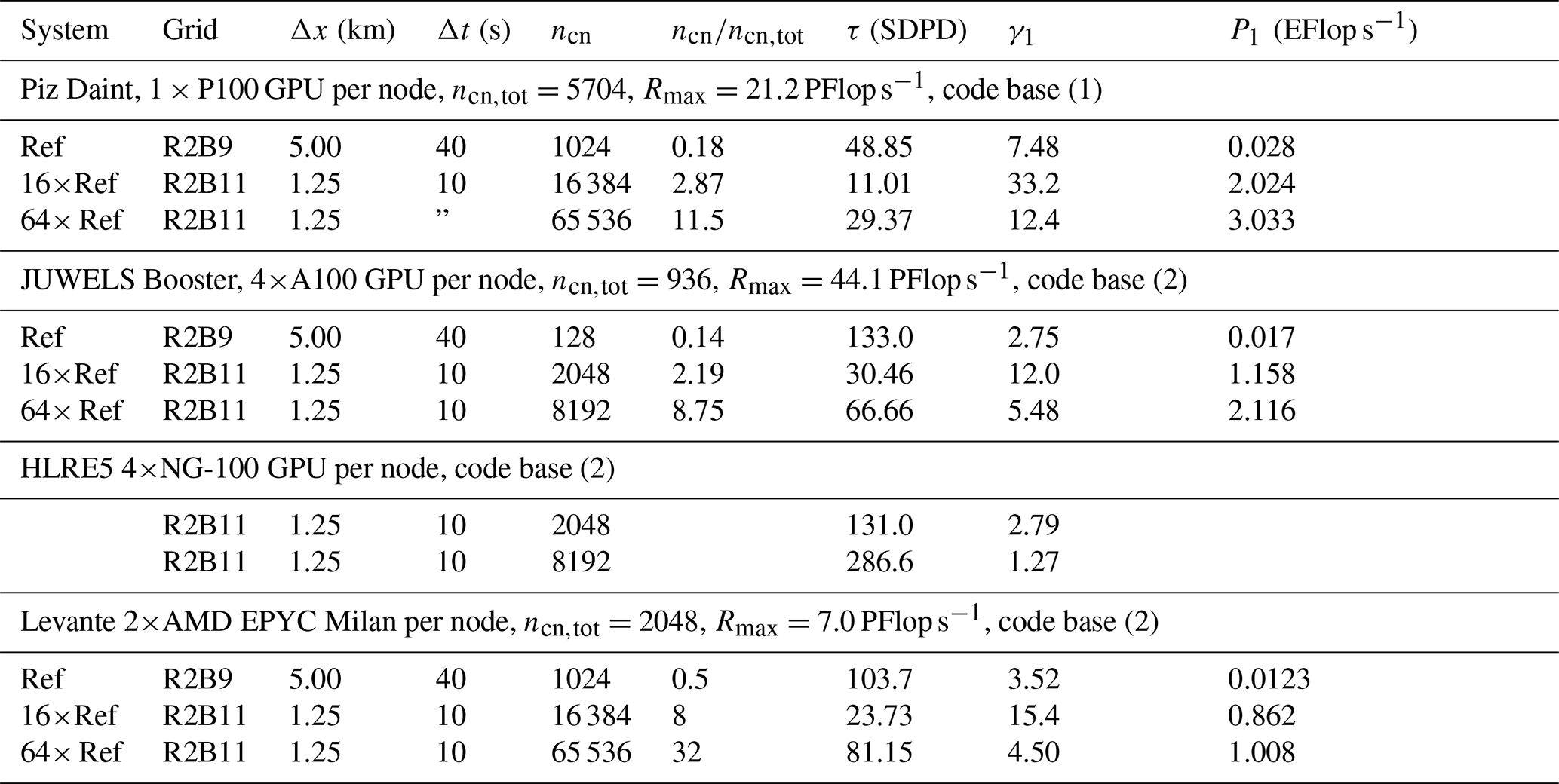
It shows that for Piz Daint, where our reference system uses only 1024 of its 5704 nodes, a system roughly 12-fold larger than Piz Daint would still fall a factor 12 short of the desired compression. This factor is too large to be achieved by further strong scaling. We get closer with the A100 chip-set, as a system roughly 9 times larger than JUWELS Booster () leads to less than a factor of 6 shortfall in temporal compression. Also this factor is out of reach given the strong scaling found on JUWELS Booster. The system gets closer not just by being bigger, but also because of the better usage of the compute power, characterized here by the LINPACK Rmax. For the Ref and 16×Ref setups, the minimum required compute power, as measured by P1, is 1.7 times reduced on JUWELS Booster compared to Piz Daint. Even if the radiation costs on Piz Daint were reduced by 60 % due to fewer g-points and computing no clear-sky radiation (and assuming the scaling remains unchanged), P1 on JUWELS Booster would still be reduced by 1.5 times. This higher efficiency is only partly explained by the 30 % increase in the counter-gradient versus LINPACK performance of JUWELS Booster versus Piz Daint.
For the CPU chipset of Levante, it is found that the 64×Ref setup would fall a factor 4.5 short of the targeted compression, and the required system would be 104 times the size of Levante. The estimate for 16×Ref on Levante may be compared to that of Neumann et al. (2019), which was based on similar ICON simulations (Δx=5 km, 90 levels, Δt=45 s), albeit with a different implementation of the physical processes. Their benchmarks were performed on the Mistral computer at DKRZ (now being replaced by Levante), using the partition with two Broadwell CPUs per node. Scaling of their performance of 26 SDPD on 256 Mistral–Broadwell nodes (their Fig. 4), and assuming an Rmax of 1.8715 PFlop s−1 for the 1714-node Broadwell partition1, yields an estimate2 of P1=0.655 EFlop s−1. This is somewhat better than what is realized on Levante, a difference that might be related to an initial, and hence sub-optimal, Levante implementation, as well as slight differences in the configuration of physical processes, for instance, the treatment of radiative transfer. However, it seems reasonable to conclude that we are not seeing a large reduction in P1 in transitioning from the Broadwell-based Mistral machine to the Milan-based Levante. This stands in contrast to the reduction in P1 in transitioning from the P100 Piz Daint to the A100 JUWELS Booster, and while the P1 values for both GPU machines remain higher than for the CPU machines, the trend is more favorable for the GPU machines, something consistent with changes in memory bandwidth3 for the different architectures.
Strong scaling limits how much we could translate a larger machine into a reduction in γ1. For example, from Table 4 the envisioned 16×Ref version of JUWELS Booster is 2.19 times larger than the existing machine and thus would correspond to an Rmax=96.5 PFlop s−1, which is still far from the required Rmax=1.158 EFlop s−1 to achieve 1 SYPD. Were one to simply increase the size of JUWELS Booster, poor strong scaling would create the need for a proportionally larger machine, something that is measured by the increase in P1 from 1.158 EFlop s−1 for the 16×Ref implementation to 2.116 EFlop s−1 for 64×Ref (Table 4). Using these numbers, we see that 1 SYPD at R2B11 is likely not attainable with the present implementation of ICON on existing GPU architectures. The present situation is somewhat more favorable on the CPU architectures. The currently second most performant computer, Fugaku, with Rmax=442 (TOP500.org, 2021), would have γ1=2.3, if ICON operated on Fugaku at the same P1 value as for the 64×Ref setup based on Levante. A factor 2.3 larger CPU machine with Rmax=1017 seems technically within reach.
The situation for the GPU machines becomes more favorable when we look toward the future. Realizing a factor of 4.3×A100 in transitioning to a next generation GPU (NG-100 in Table 4), as found in the ICON-A benchmarks in the transition from the P100 to the A100 GPU, would imply γ1=2.78 for a 2048 node 4×NG-100 system rated at Rmax=415 PFlop s−1. For such a system, even without improvements in strong scaling, the 64×Ref benchmark on JUWELS Booster implies a γ1=1.3 and an Rmax=1660 PFlop s−1. This indicates that for the GPU architectures, performance improvement of 4.3× over the A100 would begin to out perform the CPU performance for the same Rmax.
The recently announced Nvidia Hopper GPU promises a performance increase in this range and perhaps even larger (NVIDIA, 2022). In addition, Fugaku, an exceptionally efficient CPU machine, still uses twice as much electrical power as JUWELS Booster when normalized by Rmax, which further favors GPU-based implementations of ICON in the future. The upshot of these calculations is that the goal of 1 SYPD at roughly a 1 km scale is well within reach.
6.5.3 Anticipated increases in τ from hardware
General circulation models typically process many grid points with often relatively little compute load, which results in the bandwidth limitation encountered in the single-node speedup tests. This means that improved memory bandwidth allows for a better exploitation of the compute power of the GPUs, which helps explain the considerably improved performance of ICON-A on the A100 versus the P100 GPUs
Another typical characteristic is the organization of the work, which happens in many separated loops, often with not very many operations. On the GPUs, this results in a non-negligible amount of time spent for the preparation of the parallel regions. If this amount remains constant while the computation decreases with increasing parallelization, then the benefit of stronger parallelization will be limited. Similarly, if a newer system has increased compute speed but still spends the same time for the overhead for GPU kernels, then ICON cannot profit that much. Thus, in the absence of refactoring, to realize the benefits of an acceleration of the GPU compute speed would require a commensurate speedup of the overhead time for the GPU-parallel regions.
6.5.4 Anticipated increases in τ from software
Because the scaling and computational throughput are limited by the dynamical core, algorithmic improvements to this component of the code, followed by the transport scheme, stand the best chance of increasing τ. This part of the model is, however, already relatively well optimized – given the limits of what can be accomplished with openACC. Further improvements in performance would require a refactoring to exploit special features of the processors. For instance, exposing solvers to the application of AI arithmetic, i.e., matrix multiply and accumulate, where possible, could substantially improve throughput. Obviously the very poor scaling of the land scheme is also a matter of concern, though it is unclear how the underlying problems – little computational work – can be resolved.
Another, and perhaps the best, possibility to speed up the code concerns the precision of the variables and computations. ICON uses by default 64-bit variables and arithmetic, although the ICON model can be used in a mixed-precision mode, in which mostly the dynamics is computed with 32-bit arithmetic, while the remaining model components still work with 64-bit arithmetic. Because this mixed mode has not been validated on GPUs, the mixed mode is not used in this study, neither on GPU nor on CPU, although on the latter, ICON applications frequently make use of this option. Hence we see considerable potential to speed up simulations using 32-bit variables and arithmetic. Even as few as 16 bits can be sufficient if round-off errors are kept under control, as shown in Klöwer et al. (2022) for a shallow water model. This would not only speed up the simulations, but also reduce the memory footprint so that a certain turnover can be achieved with significantly fewer nodes. However, more model development would be needed to explore the potential compute time or memory savings and the effects on the simulations.
An open question is if a different parallelization would improve the turnover for a given number of nodes. The current parallelization is organized as a single geographical domain decomposition used for all model processes (and a separate decomposition for the output scheme). Thus all model processes in a domain are computed in a specified sequence by the same processor. The practical sequence of the computations of processes is determined by the order of the processes in the coupling scheme of the model. This method balances the total work to be done in each domain relatively well. But the single processes can be quite different in their work load, and, as seen above, this results in a quite uneven strong scaling behavior on GPUs. Would this be better in a process-specific parallelization, in which each process has its own domain decomposition? Such a parallelization would focus the resources on the more expensive components, and it would avoid higher parallelization of processes where the scaling limit is reached. It would also require a more complex communication scheme and an ability to compute different processes in parallel; the latter can make it difficult to maintain physical limits in tendencies, for instance, to maintain positivity of tracers. While these ideas have not yet been developed or tested in ICON, they could provide a substantial speedup in the future.
Finally it is important to verify the utility of the new model code for the QUBICC experiments, for which a small selection of results is presented here relating to two experiments performed on Piz Daint. (A more detailed analysis will be published elsewhere.) The main questions to be addressed in the beginning are the following:
-
Is the model stable over at least 1 month?
-
Are there obvious biases which need to be corrected before scientific experiments can begin?
-
Can the model simulate a reasonable tropical precipitation and the downward propagation of the QBO jet as a result of wave–mean flow interaction?
The initial series of experiments was integrated over 1 month starting from four initial dates (1 April 2004, 1 November 2004, 1 April 2005, and 1 November 2005), which were selected based on the protocol for the QBOi experiments (Butchart et al., 2018). These dates spread across a fairly normal QBO cycle, which is used here as well as in the QBOi project (Butchart et al., 2018). A second series of experiments (“dy experiments”) was conducted to investigate the issues identified in the first one.
A key learning point from the first series of experiments was that all experiments remained stable over 1 month. Therefore, the first experiment with a start date of 1 April 2004 was continued until it crashed after 2 months and 6 d with too high a wind speed at the model top. The analysis showed that not only this experiment, but also the other three experiments of this series had a tendency towards a nearly vertical axis of the polar night jet, with a very strong wind maximum found at the top of the model. A vertical jet axis with a wind maximum at ca. 80 km height is in disagreement with observations, and the high wind speeds pose a threat for numerical stability. This issue was addressed in a number of short experiments of the second series. These experiments showed that the Rayleigh damping of the vertical wind in the uppermost ca. 30 km of the model domain was too strong. An increase of the start level of the Rayleigh damping from 42 to 50 km and a reduction of the strength to 20 % of the original value lead to a more realistic wind maximum of the polar night jet at heights of 50 to 60 km.
Another important finding from the first series of experiments was that the parameterized vertical diffusion was clearly too strong. This not only slowly damped the QBO jet, but also affected many aspects of the tropospheric circulation, including the distribution and intensity of precipitation and convection. In the investigation of this problem it was found that the maximum mixing length within the vertical diffusion scheme was implemented in the code at a much larger value, 1000 m, than described in the original description, 150 m (Pithan et al., 2015). The value that is too high was reset in the experiment dy21, which ultimately reduced many large biases. Figure 8 shows the occurrence frequency for equatorial 3-hourly precipitation in the dy21 experiment, now fitting reasonably well to TRMM data (Huffman et al., 2007). In comparison, ERA5 (Hersbach et al., 2020) has more frequent weak precipitation and less frequent strong precipitation.
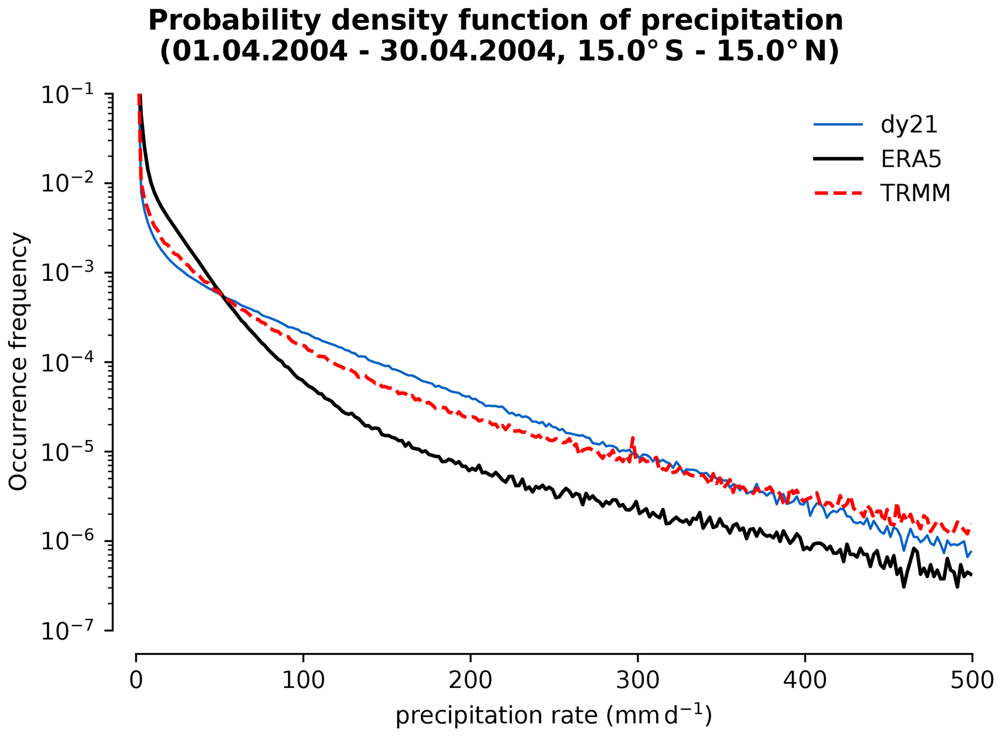
Figure 8Occurrence frequency of the 3 h mean precipitation rate between 15∘ S and 15∘ N from 1 to 30 April 2004 in the QUBICC simulation dy21, in ERA5, and in TRMM, using 250 bins of 2 mm d−1 width.
In contrast to the first series of experiments, the dy21 experiment also shows a downward propagation of the zonal mean zonal wind in the equatorial stratosphere, thus a downward progression of the westerly and easterly QBO jets, which are initially centered at ca. 30 and 40 km height, respectively (Fig. 9). However, in comparison to ERA5, the downward propagation of the easterly jet in dy21 is clearly faster, which results in growing differences in the zonal mean zonal wind in the upper half of this region. Nevertheless, the key result is that a downward propagation of the QBO jets is simulated.
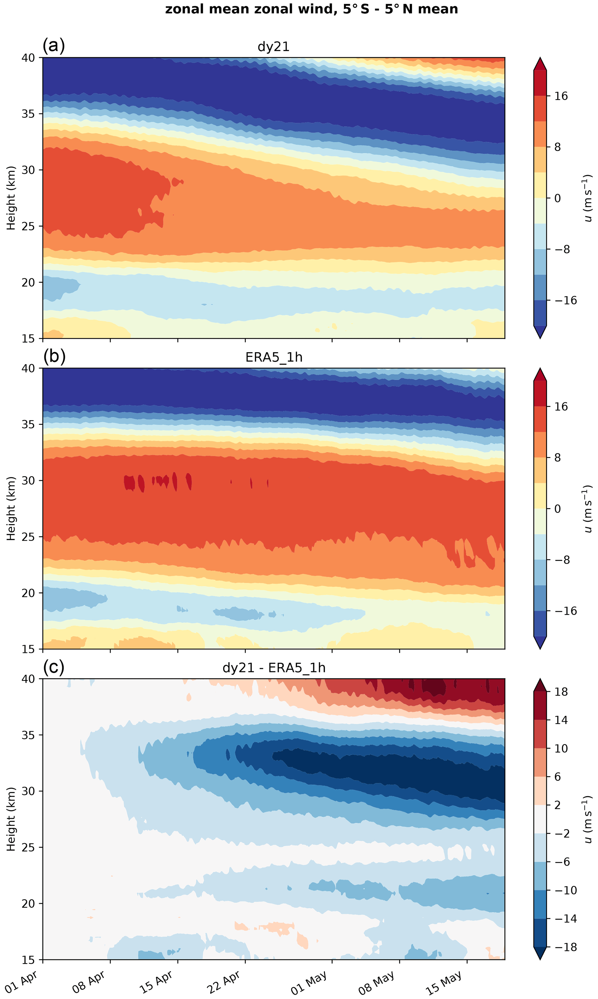
Figure 9Zonal mean zonal wind averaged from 5∘ S to 5∘ N from 1 January to 20 May 2004 in the simulation dy21 (a) and ERA5 (b) and the difference between dy21 and ERA5.
The processes which cause this downward propagation of the QBO jets include the interaction of vertically propagating waves in equatorial latitudes with these jets and their vertical advection. The contribution of these processes to the tendency of the zonal mean zonal wind can be estimated from the divergence of the Eliassen–Palm flux (EP flux) and the residual circulation in the meridional plain (see, for example, Andrews et al., 1987). For this diagnostics, the simulation data as well as the ERA5 data were first interpolated to a Gaussian grid with 1024 latitude × 512 latitude. Figure 10 shows the tendency of and the contributions from the EP flux divergences and the advection terms averaged over the first month.
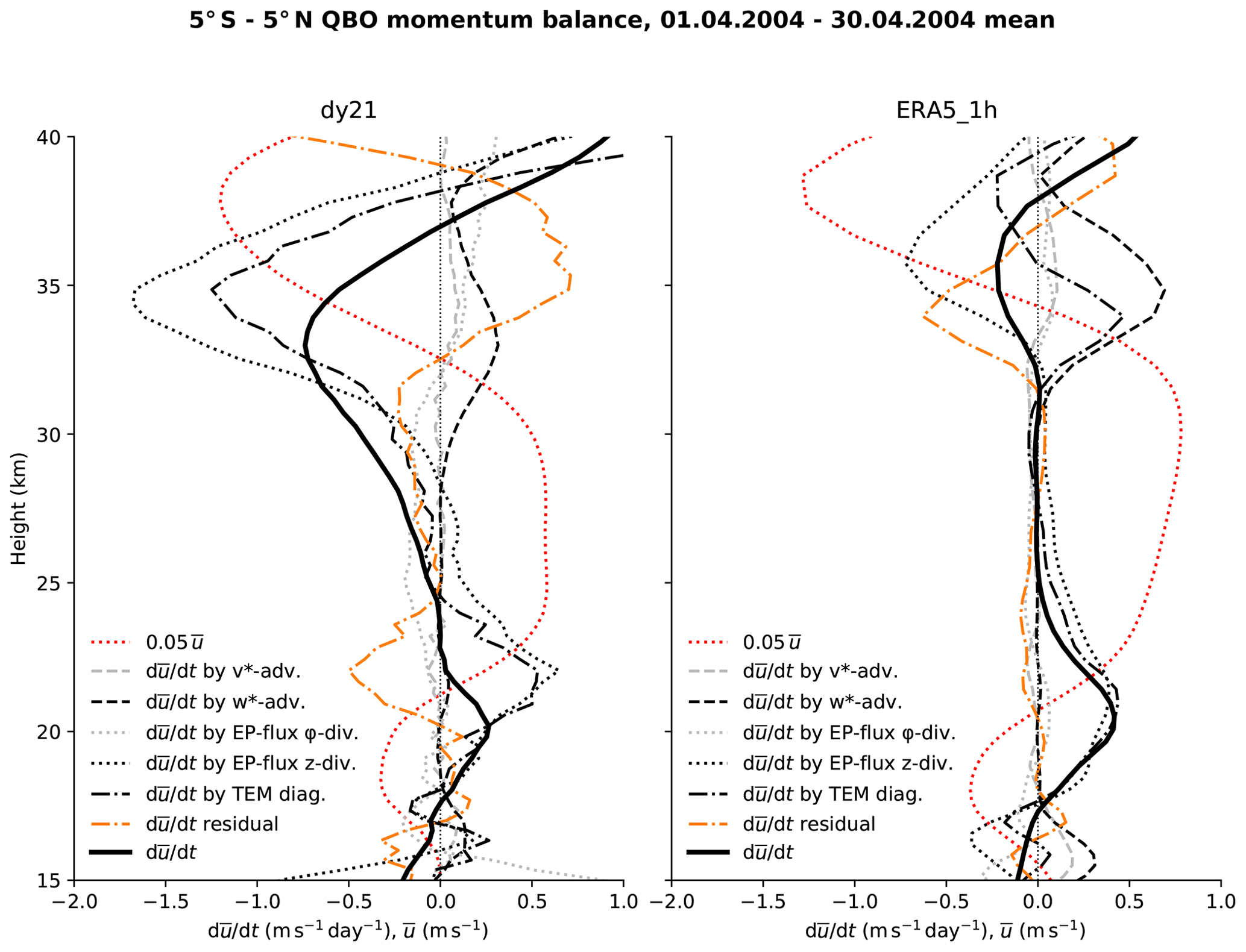
Figure 10Zonal mean zonal wind (dotted red line) and its tendencies averaged between 5∘ S and 5∘ N and between 1 and 30 April 2004 from 15 to 40 km height in the simulation dy21 and in ERA5, with the total tendency (bold line) and contributions diagnosed in the transformed Eulerian mean framework for advection by the residual meridional v* and vertical wind w* (dashed lines), the meridional and vertical divergence of the Eliassen–Palm flux (dotted lines), the sum of these four terms (dotted–dashed line), and the residual (dotted–dashed orange line).
Over this first month, the profiles of the zonal mean zonal wind () remain quite similar, except for the easterly jet centered at 40 km altitude that extends already further down in dy21. The total tendency () profile is also comparable up to 27 km but diverges above with a large negative tendency in dy21 maximizing at 33 km height, where the easterly jet has started its decent, while ERA5 shows a weaker negative tendency centered higher at 36 km height.
Below 30 km altitude the total tendency in ERA5 is mostly explained by the vertical divergence of the EP flux, (), which is almost identical to the total contribution by the EP flux divergence and the advection terms (). These tendencies appear in similar shape in dy21. Thus for the wave–mean flow interaction and the advection, as captured by this diagnostics, the simulation is close to the reanalysis. A difference exist however in the residual term (), which at these altitudes is negligible in ERA5 but significant in dy21, opposing the diagnosed vertical divergence of the EP flux. This residual term is the main reason for the difference in the total tendency between dy21 and ERA5.
Above 30 km altitude, where the easterly jet has propagated further downward in dy21 than in ERA5, is negative and peaks in the lower shear layer of the easterly jet, with a stronger amplitude in the simulation. The upward vertical wind, which creates a positive tendency in the same shear layer, however, is stronger in ERA5 than in dy21. Stronger differences exist however in the residuals, which also play a role here in ERA5. The residual tendencies make a substantial contribution to dy21 and ERA5, albeit with a vertical downward shift in the simulation. The meridional EP flux divergence as well as the meridional advection play only minor roles.
The initial sets of experiments thus led to a model version in which the wave–mean flow interaction and the advection by the residual meridional circulation play an important role. The nature of the residual terms is not yet known. But these simulations build the base for further research on the factors that influence the processes of the QBO. Eventually, with sufficient resources, this will also allow for the simulation of full QBO cycles.
With the scientific motivation to conduct a first direct simulation of the QBO relying only on explicitly resolved convection and gravity waves, the ICON atmosphere model has been ported to GPUs with all components needed for such a simulation at a horizontal resolution of 5 km and with 191 levels up to a height of 83 km. The initial GPU port of ICON on Piz Daint at CSCS is based on OpenACC directives. Benchmark experiments showed a single-node CPU-to-GPU speedup of 6.4, corresponding to the ratio of the GPU bandwidth to the CPU bandwidth. This memory bandwidth limitation of the ICON code is a typical characteristic for general circulation models. The strong scaling tests showed that a minimum of ca. 10 000 grid columns is needed on the GPU to remain efficient, which limits the possibilities to profit from strong scaling. On CPUs the limit is near 100 grid columns, which increases the strong scaling to larger processor counts. The weak scaling of ICON-A is very good (typically 0.98) over the tested 16-fold increase in grid size and node count, on both GPU and CPU architectures, making even higher resolved global simulations possible, albeit with the throughput limited by the strong scaling and the required reduction in the model time step.
For the model setup used in the QBO simulations, a turnover of 48 SDPD and 133 SDPD was achieved on the GPU systems Piz Daint at CSCS and JUWELS Booster at FZJ, respectively, while 103 SDPD were achieved on the CPU system Levante at DKRZ. Extrapolations show that ICON simulations at 1.25 km resolution and 1 SYPD turnover will be possible on the next generation of supercomputers.
The GPU port of ICON-A made the first series of experiments related to the QBO processes possible. These experiments led to a better tuning of the damping and diffusion schemes, which in the end allowed for a first simulation showing downward-propagating QBO jets driven by wave–mean flow interaction in a model where the tropical wave spectrum depends entirely on explicitly simulated convection. However, further research is needed to understand why the downward propagation of the easterly jet was too fast. As in the case of the QBO, other scientific problems in climate research which depend on scales from a few kilometers or smaller to the global scale will also need enormous computational resources. Having now a code that can be used on the largest supercomputers using GPUs will open up new opportunities in this direction.
The codes (1) and (2) listed in Table 2 and the run scripts for Piz Daint, JUWELS Booster, and Levante are available in the related data repository (https://doi.org/10.17617/3.5CYUFN, Giorgetta, 2022). These code versions are not standard release versions, but the related GPU developments are merged in the release candidate for the upcoming release version icon-2.6.5. Release versions of the code are available to individuals under license as described by MPI-M (2022). By downloading the ICON source code, the user accepts the license agreement.
The data relating to the vertical grid (Fig. 1), codes (Table 2), computers (Table 4), speedup (Fig. 4), strong scaling (Fig. 6), time to solution and scaling (Table 3 and Fig. 5), turnover rate (Table 3, Fig. 7), and outlook (Table 4) are stored in the data.ods spreadsheet of the related data repository (https://doi.org/10.17617/3.5CYUFN; Giorgetta, 2022).
MAG guided the presented work from the experimental side, made the benchmark and QUBICC simulations on Piz Daint and JUWELS Booster, and led the writing of the manuscript as a whole. WS, DA, RP, and RS wrote parts of the manuscript. MAG and HF worked on the evaluation of the QUBICC experiment. WS developed the GPU port of most parts of the dynamical core and the transport scheme, with additional contributions from DR. XL and PM ported most of the atmospheric physics parameterization. ME implemented and ported the graupel cloud microphysics scheme. VC and RS developed the GPU port of the land physics and the CLAW tool needed for this purpose. RP and SR contributed with the RTE+RRTMGP radiation scheme and its interfaces to ICON, while MRN, BRH, and WMH contributed to the initial development of the RTE+RRTMGP GPU implementation. DA refined and optimized the GPU-enabled ICON code, especially with regard to the communication and specifics of the compilers. He also optimized the GPU port for JUWELS Booster. RD developed the tolerance test procedure. LK, US, JFE, and PA contributed to the I/O scheme, and LK prepared the initial and external parameter files for the experiments. CF made the benchmark runs on the Levante computer at DKRZ. BS initiated the PASC ENIAC project for the GPU port and contributed to the analysis of Sect. 6 and to the writing of the manuscript as a whole.
The contact author has declared that none of the authors has any competing interests.
Publisher's note: Copernicus Publications remains neutral with regard to jurisdictional claims in published maps and institutional affiliations.
We acknowledge PRACE for awarding us access to Piz Daint at the Swiss National Supercomputing Centre and JUWELS Booster at the Forschungszentrum Jülich (allocation no. 2019215178). Thomas Schulthess at CSCS generously supported the development of the GPU port of ICON with staff and additional computational resources on Piz Daint, especially during the transition from Piz Daint to JUWELS Booster. We are grateful to Italo Epicoco and an anonymous reviewer for their comments in EGUsphere and to Leonidas Linardakis for the internal review at MPI-M.
Philippe Marti and Valentin Clément received funding from the Platform for Advanced Scientific
Computing (PASC) of ETH (reference number 2017-8). Some portions of the work of Matthew R. Norman,
Benjamin R. Hillman, and Walter M. Hannah on RTE+RRTMGP were funded by the US Department of Energy (grant no. DE-SC0021262) and by Lawrence Livermore National Laboratory (contract no. DE-AC52-07NA27344).
The article processing charges for this open-access publication were covered by the Max Planck Society.
This paper was edited by Sophie Valcke and reviewed by Italo Epicoco and one anonymous referee.
Andrews, D. G., Holton, J. R., and Leovy, C. B.: Middle Atmosphere Dynamics, Academic Press, https://doi.org/10.1002/qj.49711548612, 1987. a
Anstey, J. A., Osprey, S. M., Alexander, J., Baldwin, M. P., Butchart, N., Gray, L., Kawatani, Y., Newman, P. A., and Richter, J. H.: Impacts, processes and projections of the quasi-biennial oscillation, Nature Reviews Earth & Environment, 3, 588–603, https://doi.org/10.1038/s43017-022-00323-7, 2022. a
Baldwin, M. P., Gray, L. J., Dunkerton, T. J., Hamilton, K., Haynes, P. H., Randel, W. J., Holton, J. R., Alexander, M. J., Hirota, I., Horinouchi, T., Jones, D. B. A., Kinnersley, J. S., Marquardt, C., Sato, K., and Takahashi, M.: The quasi-biennial oscillation, Rev. Geophys., 39, 179–229, https://doi.org/10.1029/1999RG000073, 2001. a
Butchart, N., Anstey, J. A., Hamilton, K., Osprey, S., McLandress, C., Bushell, A. C., Kawatani, Y., Kim, Y.-H., Lott, F., Scinocca, J., Stockdale, T. N., Andrews, M., Bellprat, O., Braesicke, P., Cagnazzo, C., Chen, C.-C., Chun, H.-Y., Dobrynin, M., Garcia, R. R., Garcia-Serrano, J., Gray, L. J., Holt, L., Kerzenmacher, T., Naoe, H., Pohlmann, H., Richter, J. H., Scaife, A. A., Schenzinger, V., Serva, F., Versick, S., Watanabe, S., Yoshida, K., and Yukimoto, S.: Overview of experiment design and comparison of models participating in phase 1 of the SPARC Quasi-Biennial Oscillation initiative (QBOi), Geosci. Model Dev., 11, 1009–1032, https://doi.org/10.5194/gmd-11-1009-2018, 2018. a, b
Clement, V., Ferrachat, S., Fuhrer, O., Lapillonne, X., Osuna, C. E., Pincus, R., Rood, J., and Sawyer, W.: The CLAWDSL: Abstractions for performance portable weather and climate models, Proceedings of the Platform for Advanced Scientific Computing Conference, PASC 2018, 2, 1–10, https://doi.org/10.1145/3218176.3218226, 2018. a, b
Clement, V., Marti, P., Fuhrer, O., Sawyer, W., and Lapillonne, X.: Automatic Port to OpenACC/OpenMP for Physical Parameterization in Climate and Weather Code Using the CLAW Compiler, Supercomputing Frontiers and Innovations, 6, 51–63, https://doi.org/10.14529/jsfi190303, 2019. a, b, c
CSCS: Piz Daint, https://www.cscs.ch/computers/piz-daint/, last access: 18 March 2022. a
Demeshko, I., Maruyama, N., Tomita, H., and Matsuoka, S.: Multi-GPU Implementation of the NICAM Atmospheric Model, in: Euro-Par 2012: Parallel Processing Workshops, edited by: Caragiannis, I., Alexander, M., Badia, R. M., Cannataro, M., Costan, A., Danelutto, M., Desprez, F., Krammer, B., Sahuquillo, J., Scott, S. L., and Weidendorfer, J., Springer Berlin Heidelberg, Berlin, Heidelberg, 175–184, https://doi.org/10.1007/978-3-642-36949-0, 2013. a
DKRZ: HLRE-4 Levante, https://www.dkrz.de/en/systems/hpc/hlre-4-levante, last access: 18 March 2022. a
Doms, G., Förstner, J., Heise, E., Herzog, H.-J., Mironov, D., Raschendorfer, M., Reinhardt, T., Ritter, B., Schrodin, R., Schulz, J.-P., and Vogel, G.: A Description of the Nonhydrostatic Regional COSMO Model Part II: Physical Parameterization, Tech. rep., Deutscher Wetterdienst, https://www.cosmo-model.org/content/model/documentation/core/cosmo_physics_4.20.pdf (last access: 10 September 2022), 2011. a
Fuhrer, O., Chadha, T., Hoefler, T., Kwasniewski, G., Lapillonne, X., Leutwyler, D., Lüthi, D., Osuna, C., Schär, C., Schulthess, T. C., and Vogt, H.: Near-global climate simulation at 1 km resolution: establishing a performance baseline on 4888 GPUs with COSMO 5.0, Geosci. Model Dev., 11, 1665–1681, https://doi.org/10.5194/gmd-11-1665-2018, 2018. a
FZJ: Hardware Configuration of the JUWELS Booster Module, https://apps.fz-juelich.de/jsc/hps/juwels/configuration.html#hardware-configuration-of-the-system-name-booster-module, last access: 18 March 2021. a
Gheller, C.: D8.4.2: Final Refactoring Report, Tech. rep., PRACE-2IP, https://prace-ri.eu/about/ip-projects/public-deliverables/#PRACE2IP (last access: 10 September 2022), 2014. a
Giorgetta, M. A.: The ICON-A model for direct QBO simulations on GPUs, Edmond – The Open Research Data Repository of the Max Planck Society [code and data], https://doi.org/10.17617/3.5CYUFN, 2022. a
Giorgetta, M. A., Brokopf, R., Crueger, T., Esch, M., Fiedler, S., Helmert, J., Hohenegger, C., Kornblueh, L., Kohler, M., Manzini, E., Mauritsen, T., Nam, C., Raddatz, T., Rast, S., Reinert, D., Sakradzija, M., Schmidt, H., Schneck, R., Schnur, R., Silvers, L., Wan, H., Zangl, G., and Stevens, B.: ICON-A, the Atmosphere Component of the ICON Earth System Model: I. Model Description, J. Adv. Model. Earth Sy., 10, 1613–1637, https://doi.org/10.1029/2017ms001242, 2018. a, b, c, d, e, f, g, h, i, j, k
Govett, M., Rosinski, J., Middlecoff, J., Henderson, T., Lee, J., MacDonald, A., Wang, N., Madden, P., Schramm, J., and Duarte, A.: Parallelization and Performance of the NIM Weather Model on CPU, GPU, and MIC Processors, B. Am. Meteorol. Soc., 98, 2201–2213, https://doi.org/10.1175/BAMS-D-15-00278.1, 2017. a
Hersbach, H., Bell, B., Berrisford, P., Hirahara, S., Horányi, A., Muñoz-Sabater, J., Nicolas, J., Peubey, C., Radu, R., Schepers, D., Simmons, A., Soci, C., Abdalla, S., Abellan, X., Balsamo, G., Bechtold, P., Biavati, G., Bidlot, J., Bonavita, M., De Chiara, G., Dahlgren, P., Dee, D., Diamantakis, M., Dragani, R., Flemming, J., Forbes, R., Fuentes, M., Geer, A., Haimberger, L., Healy, S., Hogan, R. J., Hólm, E., Janisková, M., Keeley, S., Laloyaux, P., Lopez, P., Lupu, C., Radnoti, G., de Rosnay, P., Rozum, I., Vamborg, F., Villaume, S., and Thépaut, J.-N.: The ERA5 global reanalysis, Q. J. Roy. Meteor. Soc., 146, 1999–2049, https://doi.org/10.1002/qj.3803, 2020. a
Hohenegger, C., Kornblueh, L., Klocke, D., Becker, T., Cioni, G., Engels, J. F., Schulzweida, U., and Stevens, B.: Climate Statistics in Global Simulations of the Atmosphere, from 80 to 2.5 km Grid Spacing, J. Meteorol. Soc. Jpn. Ser. II, 98, 73–91, https://doi.org/10.2151/jmsj.2020-005, 2020. a, b, c
Huang, M., Mielikainen, J., Huang, B., Chen, H., Huang, H.-L. A., and Goldberg, M. D.: Development of efficient GPU parallelization of WRF Yonsei University planetary boundary layer scheme, Geosci. Model Dev., 8, 2977–2990, https://doi.org/10.5194/gmd-8-2977-2015, 2015. a
Huffman, G. J., Bolvin, D. T., Nelkin, E. J., Wolff, D. B., Adler, R. F., Gu, G., Hong, Y., Bowman, K. P., and Stocker, E. F.: The TRMM Multisatellite Precipitation Analysis (TMPA): Quasi-Global, Multiyear, Combined-Sensor Precipitation Estimates at Fine Scales, J. Hydrometeorol., 8, 38–55, https://doi.org/10.1175/JHM560.1, 2007. a
Kim, J. Y., Kang, J.-S., and Joh, M.: GPU acceleration of MPAS microphysics WSM6 using OpenACC directives: Performance and verification, Comput. Geosci., 146, 104627, https://doi.org/10.1016/j.cageo.2020.104627, 2021. a
Klemp, J. B., Dudhia, J., and Hassiotis, A. D.: An Upper Gravity-Wave Absorbing Layer for NWP Applications, Mon. Weather Rev., 136, 3987–4004, https://doi.org/10.1175/2008MWR2596.1, 2008. a
Klöwer, M., Hatfield, S., Croci, M., Düben, P. D., and Palmer, T. N.: Fluid Simulations Accelerated With 16 Bits: Approaching 4x Speedup on A64FX by Squeezing ShallowWaters.jl Into Float16, J. Adv. Model. Earth Sy., 14, e2021MS002684, https://doi.org/10.1029/2021MS002684, 2022. a
Leuenberger, D., Koller, M., Fuhrer, O., and Schär, C.: A Generalization of the SLEVE Vertical Coordinate, Mon. Weather Rev., 138, 3683–3689, https://doi.org/10.1175/2010MWR3307.1, 2010. a
Mauritsen, T., Svensson, G., Zilitinkevich, S. S., Esau, I., Enger, L., and Grisogono, B.: A Total Turbulent Energy Closure Model for Neutrally and Stably Stratified Atmospheric Boundary Layers, J. Atmos. Sci., 64, 4113–4126, https://doi.org/10.1175/2007JAS2294.1, 2007. a
Meinshausen, M., Vogel, E., Nauels, A., Lorbacher, K., Meinshausen, N., Etheridge, D. M., Fraser, P. J., Montzka, S. A., Rayner, P. J., Trudinger, C. M., Krummel, P. B., Beyerle, U., Canadell, J. G., Daniel, J. S., Enting, I. G., Law, R. M., Lunder, C. R., O'Doherty, S., Prinn, R. G., Reimann, S., Rubino, M., Velders, G. J. M., Vollmer, M. K., Wang, R. H. J., and Weiss, R.: Historical greenhouse gas concentrations for climate modelling (CMIP6), Geosci. Model Dev., 10, 2057–2116, https://doi.org/10.5194/gmd-10-2057-2017, 2017. a
MPI-M: https://mpimet.mpg.de/en/science/modeling-with-icon/code-availability, last access: 10 September 2022.
Müller, S. K., Manzini, E., Giorgetta, M., Sato, K., and Nasuno, T.: Convectively Generated Gravity Waves in High Resolution Models of Tropical Dynamics, J. Adv. Model. Earth Sy., 10, 2564–2588, https://doi.org/10.1029/2018MS001390, 2018. a
Neumann, P., Düben, P., Adamidis, P., Bauer, P., Brück, M., Kornblueh, L., Klocke, D., Stevens, B., Wedi, N., and Biercamp, J.: Assessing the scales in numerical weather and climate predictions: will exascale be the rescue?, Philos. T. R. Soc. A, 377, 20180148, https://doi.org/10.1098/rsta.2018.0148, 2019. a
NVIDIA: NVIDIA H100 Tensor Core GPU, https://www.nvidia.com/en-us/data-center/h100/, last access: 23 March 2022. a
Pincus, R. and Stevens, B.: Paths to accuracy for radiation parameterizations in atmospheric models, J. Adv. Model. Earth Sy., 5, 225–233, https://doi.org/10.1002/jame.20027, 2013. a
Pincus, R., Mlawer, E. J., and Delamere, J. S.: Balancing Accuracy, Efficiency, and Flexibility in Radiation Calculations for Dynamical Models, J. Adv. Model. Earth Sy., 11, 3074–3089, https://doi.org/10.1029/2019MS001621, 2019. a, b
Pithan, F., Angevine, W., and Mauritsen, T.: Improving a global model from the boundary layer: Total turbulent energy and the neutral limit Prandtl number, J. Adv. Model. Earth Sy., 7, 791–805, https://doi.org/10.1002/2014MS000382, 2015. a
Reick, C. H., Gayler, V., Goll, D., Hagemann, S., Heidkamp, M., Nabel, J. E. M. S., Raddatz, T., Roeckner, E., Schnur, R., and Wilkenskjeld, S.: JSBACH 3 – The land component of the MPI Earth System Model: Documentation of version 3.2, Berichte zur Erdsystemforschung, 240, 287, https://doi.org/10.17617/2.3279802, 2021. a
Reinert, D.: The Tracer Transport Module Part I: A Mass Consistent Finite Volume Approach with Fractional Steps, Tech. rep., DWD, https://doi.org/10.5676/DWD_pub/nwv/icon_005, 2020. a, b
Richter, J. H., Butchart, N., Kawatani, Y., Bushell, A. C., Holt, L., Serva, F., Anstey, J., Simpson, I. R., Osprey, S., Hamilton, K., Braesicke, P., Cagnazzo, C., Chen, C.-C., Garcia, R. R., Gray, L. J., Kerzenmacher, T., Lott, F., McLandress, C., Naoe, H., Scinocca, J., Stockdale, T. N., Versick, S., Watanabe, S., Yoshida, K., and Yukimoto, S.: Response of the Quasi-Biennial Oscillation to a warming climate in global climate models, Q. J. Roy. Meteor. Soc., 148, 1490–1518, https://doi.org/10.1002/qj.3749, 2020. a
Schirber, S., Manzini, E., Krismer, T., and Giorgetta, M.: The quasi‐biennial oscillation in a warmer climate: sensitivity to different gravity wave parameterizations, Clim. Dynam., 45, 825––836, https://doi.org/10.1007/s00382-014-2314-2, 2015. a
Stephan, C. C., Strube, C., Klocke, D., Ern, M., Hoffmann, L., Preusse, P., and Schmidt, H.: Intercomparison of Gravity Waves in Global Convection-Permitting Models, J. Atmos. Sci., 76, 2739–2759, https://doi.org/10.1175/JAS-D-19-0040.1, 2019. a
Stevens, B., Giorgetta, M., Esch, M., Mauritsen, T., Crueger, T., Rast, S., Salzmann, M., Schmidt, H., Bader, J., Block, K., Brokopf, R., Fast, I., Kinne, S., Kornblueh, L., Lohmann, U., Pincus, R., Reichler, T., and Roeckner, E.: Atmospheric component of the MPI-M Earth System Model: ECHAM6, J. Adv. Model. Earth Sy., 5, 146–172, https://doi.org/10.1002/jame.20015, 2013. a
Stevens, B., Satoh, M., Auger, L., Biercamp, J., Bretherton, C. S., Chen, X., Düben, P., Judt, F., Khairoutdinov, M., Klocke, D., Kodama, C., Kornblueh, L., Lin, S.-J., Neumann, P., Putman, W. M., Röber, N., Shibuya, R., Vanniere, B., Vidale, P. L., Wedi, N., and Zhou, L.: DYAMOND: the DYnamics of the Atmospheric general circulation Modeled On Non-hydrostatic Domains, Progress in Earth and Planetary Science, 6, 61, https://doi.org/10.1186/s40645-019-0304-z, 2019. a
TOP500.org: TOP500 List November 2021, https://top500.org/lists/top500/2021/11/ (last access: 23 March 2022), 2021. a, b, c, d
Wang, P., Jiang, J., Lin, P., Ding, M., Wei, J., Zhang, F., Zhao, L., Li, Y., Yu, Z., Zheng, W., Yu, Y., Chi, X., and Liu, H.: The GPU version of LASG/IAP Climate System Ocean Model version 3 (LICOM3) under the heterogeneous-compute interface for portability (HIP) framework and its large-scale application , Geosci. Model Dev., 14, 2781–2799, https://doi.org/10.5194/gmd-14-2781-2021, 2021. a
Zängl, G., Reinert, D., Ripodas, P., and Baldauf, M.: The ICON (ICOsahedral Non-hydrostatic) modelling framework of DWD and MPI-M: Description of the non-hydrostatic dynamical core, Q. J. Roy. Meteor. Soc., 141, 563–579, https://doi.org/10.1002/qj.2378, 2015. a, b, c
TOP500 for November 2015 reported Rmax=1.1392 PFlop s−1 for 1556 Haswell nodes, and TOP500 for November 2016 reported Rmax=3.0107 PFlop s−1 for 1557 Haswell nodes + 1714 Broadwell nodes. The difference, attributed here to 1714 Broadwell nodes, is 1.8715 PFlop s−1
Here we assume perfect weak scaling, starting from the 26 SDPD for R2B9 on 256 nodes, which yields a for R2B11, with the latter (45/40) factor accounting for differences in time steps. The weak-scaling to R2B11 (using the same Sw=0.978 as for Levante) inflates the size to nodes
Memory bandwidth per core decreased by approximately 25 % on Levante relative to Mistral but increased by 10 % on JUWELS Booster as compared to Piz Daint.
- Abstract
- Introduction
- Model configuration for QUBICC experiments
- The compute systems
- Porting ICON to GPUs
- Validation
- Benchmarking results
- First QBO experiments
- Conclusions
- Code availability
- Data availability
- Author contributions
- Competing interests
- Disclaimer
- Acknowledgements
- Financial support
- Review statement
- References