Synergy between satellite observations of soil moisture and water storage anomalies for runoff estimation

This paper presents an innovative approach, STREAM – SaTellite-based Runoff Evaluation And Mapping – to derive daily river discharge and runoff estimates from satellite observations of soil moisture, precipitation, and total water storage anomalies (TWSAs). Within a very simple model structure, precipitation and soil moisture data are used to estimate the quick-flow river discharge component while TWSAs are used for obtaining its complementary part, i.e., the slow-flow river discharge component. The two are then added together to obtain river discharge estimates.

The method is tested over the Mississippi River basin for the period 2003–2016 by using precipitation data from the Tropical Rainfall Measuring Mission (TRMM) Multi-satellite Precipitation Analysis (TMPA), soil moisture data from the European Space Agency's Climate Change Initiative (ESA CCI), and total water storage data from the Gravity Recovery and Climate Experiment (GRACE). Despite the model simplicity, relatively high-performance scores are obtained in river discharge estimates, with a Kling–Gupta efficiency (KGE) index greater than 0.64 both at the basin outlet and over several inner stations used for model calibration, highlighting the high information content of satellite observations on surface processes. Potentially useful for multiple operational and scientific applications, from flood warning systems to the understanding of water cycle, the added value of the STREAM approach is twofold: (1) a simple modeling framework, potentially suitable for global runoff monitoring, at daily timescale when forced with satellite observations only, and (2) increased knowledge of natural processes and human activities as well as their interactions on the land.

1 Introduction

Spatial and temporal continuous river discharge monitoring is paramount for improving the understanding of the hydrological cycle, planning human activities related to water use, and preventing or mitigating the losses due to extreme flood events. To accomplish these tasks, runoff and river discharge data representing the aggregated signal of runoff (Fekete et al., 2012) should be available at adequate spatial and temporal resolutions. For water resources management and drought monitoring, monthly time series over basin areas larger than 10 000 km² are sufficient, whereas observations up to a grid scale of a few kilometers and daily or sub-daily time steps are required for flood prediction. The accurate spatiotemporally continuous runoff and river discharge estimation at finer spatial or temporal resolution is still a big challenge for hydrologists.

Traditional in situ observations of river discharge, even if generally characterized by high temporal resolution (up to sub-hourly time step), typically offer little information on the spatial distribution of runoff within a watershed. Moreover, river discharge observation networks suffer from many limitations, such as low station density and often incomplete temporal coverage, substantial delay in data access, and a large decline in monitoring capacity (Vörösmarty et al., 2001). Paradoxically, this latter issue is exacerbated in developing nations (Crochemore et al., 2020), where the knowledge of the terrestrial water dynamics deserves greater attention due to huge damages to settlements and especially the loss of human lives that occurs regularly.

This precarious situation has led to growing interest in finding alternative solutions, i.e., model-based or observation-based approaches, for runoff and river discharge monitoring. Model-based approaches, based on the mathematical description of the main hydrological processes (e.g., water balance models (WBMs), global hydrological models (GHMs; e.g., Döll et al., 2003), or, increasing in complexity, land surface models (LSMs; e.g., Balsamo et al., 2009; Schellekens et al., 2017), are able to provide comprehensive information on a large number of relevant variables of the hydrological cycle, including runoff and river discharge at very high temporal and spatial resolution (up to hourly sampling and 0.05^∘ grid scale). However, the values of modeled water balance components rely on a massive parameterization of the soil, vegetation, and land parameters, which is not always realistic, and are strongly dependent on GHMs or LSMs used, analysis periods (Wisser et al., 2010), and climate forcings selected (e.g., Haddeland et al., 2012; Gudmundsson et al., 2012a, b; Prudhomme et al., 2014; Müller Schmied et al., 2016).

Alternatively, the observation-based approaches exploit machine-learning techniques and a considerable amount of data to describe the physics of the system (Solomatine and Ostfeld, 2008) with only a limited number of assumptions. Despite being simpler than model-based approaches, these approaches still present some limitations. For example, they rely on a considerable amount of data describing the modeled system's physics and spatial/temporal extent, and the uncertainty of the resulting dataset is determined by both the spatiotemporal coverage and the accuracy of the forcing data (e.g., see E-RUN dataset, Gudmundsson and Seneviratne, 2016; GRUN dataset, Ghiggi et al., 2019a; FLO1K dataset, Barbarossa et al., 2018). Additional limitations stem from the employed method to estimate runoff. Indeed, random forests such as employed in Gudmundsson and Seneviratne (2016), similar to other machine-learning techniques, are powerful tools for data-driven modeling, but they are prone to overfitting, implying that noise in the data can obscure possible signals (Hastie et al., 2009). Moreover, the influence of land parameters on continental-scale runoff dynamics is not considered, as the underlying hypothesis is that the hydrological response of a basin exclusively depends on present and past atmospheric forcing. It is easy to understand that this assumption will only be valid in certain circumstances and might lead to problems, e.g., over complex terrain (Orth and Seneviratne, 2015) or in cases of human river flow regulation (Ghiggi et al., 2019a).

Remote sensing can provide estimates of nearly all the climate variables of the global hydrological cycle, including soil moisture (e.g., Wagner et al., 2007; Seneviratne et al., 2010), precipitation (Huffman et al., 2014), and total terrestrial water storage (e.g., Houborg et al., 2012; Landerer and Swenson, 2012; Famiglietti and Rodell, 2013). It has undeniably changed and dramatically improved the ability to monitor the global water cycle, and hence runoff. By taking advantage of satellite information, some studies tried to develop methodologies that are able to optimally produce multivariable datasets from the fusion of in situ and satellite-based observations (e.g., Rodell et al., 2015; Zhang et al., 2018; Pellet et al., 2019). Other studies exploited satellite observations of hydrological variables, e.g., precipitation (Hong et al., 2007), soil moisture (Massari et al., 2014), and geodetic variables (e.g., Sneeuw et al., 2014; Tourian et al., 2018) to monitor single components of the water cycle in an independent way.

Although the majority of these studies provide runoff and river discharge data at basin scale and monthly time steps, they deserve to be recalled here as important for the purpose of the present study. In particular, Hong et al. (2007) presented a first attempt to obtain an approximate but quasi-global annual streamflow dataset by incorporating satellite precipitation data in a relatively simple rainfall-runoff simulation approach. Driven by the multiyear (1998–2006) Tropical Rainfall Measuring Mission (TRMM) Multi-satellite Precipitation Analysis (TMPA), runoff was independently computed for each global land surface grid cell through the Natural Resources Conservation Service (NRCS) runoff curve number (CN) method (NRCS, 1986) and subsequently routed to the watershed outlet to predict streamflow. The results, compared to the in situ observed river discharge data, demonstrated the potential of using satellite precipitation data for diagnosing river discharge values both at global scale and for medium to large river basins. If, on the one hand, the work of Hong et al. (2007) can be considered as a pioneer study, on the other hand it presents a serious drawback within the NRCS-CN method that lacks a realistic definition of the soil moisture conditions of the catchment before flood events. This aspect is not negligible, as it is well established that soil moisture is paramount in the partitioning of precipitation into surface runoff and infiltration inside a catchment (Brocca et al., 2008). In particular, for the same rainfall amount but different values of initial soil moisture conditions, different flooding effects can occur (see e.g., Crow et al., 2005; Brocca et al., 2008; Berthet et al., 2009; Merz and Bloschl, 2009; Tramblay et al., 2010). In line with this following Brocca et al. (2009), Massari et al. (2016) presented the very first attempt to estimate global streamflow data by using satellite Soil Moisture Active and Passive (SMAP; Entekhabi et al., 2010) and Global Precipitation Measurement (GPM; Huffman et al., 2019) products. Although the validation was carried out by routing the monthly surface runoff in only a single basin in Central Italy, the obtained results suggested dedicating additional efforts in this direction.

Among the studies that use satellite observations of hydrological variables for runoff estimation, the hydro-geodetic approaches are undoubtedly worth mentioning; see e.g., Sneeuw et al. (2014) for a comprehensive overview or Lorenz et al. (2014) for an analysis of satellite-based water balance misclosures with discharge as closure term. In particular, the satellite mission Gravity Recovery And Climate Experiment (GRACE), which observed the temporal changes in the gravity field, has given a strong impetus to satellite-driven hydrology research (Tapley et al., 2019). Since temporal gravity field variations over the continents imply water storage change, GRACE was the first remote-sensing system to provide observational access to deeper groundwater storage. GRACE and its successor mission GRACE Follow-On (GRACE-FO) provide monthly snapshots of the Earth's gravity field. The temporal variation is therefore relative to the temporally mean gravity field, and hence the time variations of water storage are fundamentally relative to the mean storage. This relative water storage variation is termed total water storage anomaly (TWSA).

The relation between GRACE-derived TWSA and runoff was characterized by Riegger and Tourian (2014), and even allowed the quantification of absolute drainable water storage over the Amazon (Tourian et al., 2018). In essence, the storage–runoff relation describes the gravity-driven drainage of a basin, and hence the slow-flow processes. Due to GRACE's spatiotemporal resolution, runoff and river discharge are generally available for basins larger than 160 000 km² and at monthly time steps, although sensitivity down to 64 000 km² has been demonstrated with careful post-processing (Vishwakarma et al., 2018).

Based on the above discussion, it is clear that each approach presents strengths and limitations that enable or hamper the runoff and river discharge monitoring at finer spatiotemporal resolutions. In this context, this study presents an attempt to find an alternative method to derive daily river discharge and runoff estimates at 0.25^∘ spatial resolution, exploiting satellite observations and the knowledge of the key mechanisms and processes that act in the formation of runoff, i.e., the role of soil moisture in determining the response of a catchment to precipitation. For that, soil moisture, precipitation, and TWSA observations are used as input into a simple modeling framework named STREAM v1.3 (SaTellite-based Runoff Evaluation And Mapping, version 1.3, hereafter referred to as STREAM). Unlike classical LSMs, STREAM exploits the knowledge of the system states (i.e., soil moisture and TWSA) to derive river discharge and runoff, and thus it (1) skips the modeling of the evapotranspiration fluxes which are known to be a non-negligible source of uncertainty (Long et al., 2014), (2) limits the uncertainty associated with the over-parameterization of soil and land parameters, and (3) implicitly takes into account processes, mainly human-driven (e.g., irrigation, change in the land use), that might have a large impact on the hydrological cycle and hence on runoff.

A detailed description of the STREAM model is given in Sect. 4. The collected datasets and the experimental design for the Mississippi River basin (Sect. 2) are described in Sects. 3 and 5, respectively. Results, discussion, and conclusions are drawn in Sects. 6–8, respectively.

2 Study area

The STREAM model presented here has been tested and validated over the Mississippi River basin (Fig. 1a). With a drainage area of about 3.3×10⁶ km², the Mississippi River basin is the fourth largest watershed in the world, bordered to the west by the crest of the Rocky Mountains and to the east by the crest of the Appalachian Mountains. According to the Köppen climate classification, the climate is subtropical humid over the southern part of the basin, continental humid with hot summer over the central part, continental humid with warm summer over the eastern and northern parts, whereas a semiarid cold climate affects the western part. The average annual air temperature across the watershed ranges from 4 ^∘C in the west to 6 ^∘C in the east. On average, the watershed receives about 900 mm yr⁻¹ of precipitation (77 % as rainfall and 23 % as snowfall), more concentrated in the eastern and southern parts of the basin in relation to its northern and western parts (Vose et al., 2014).

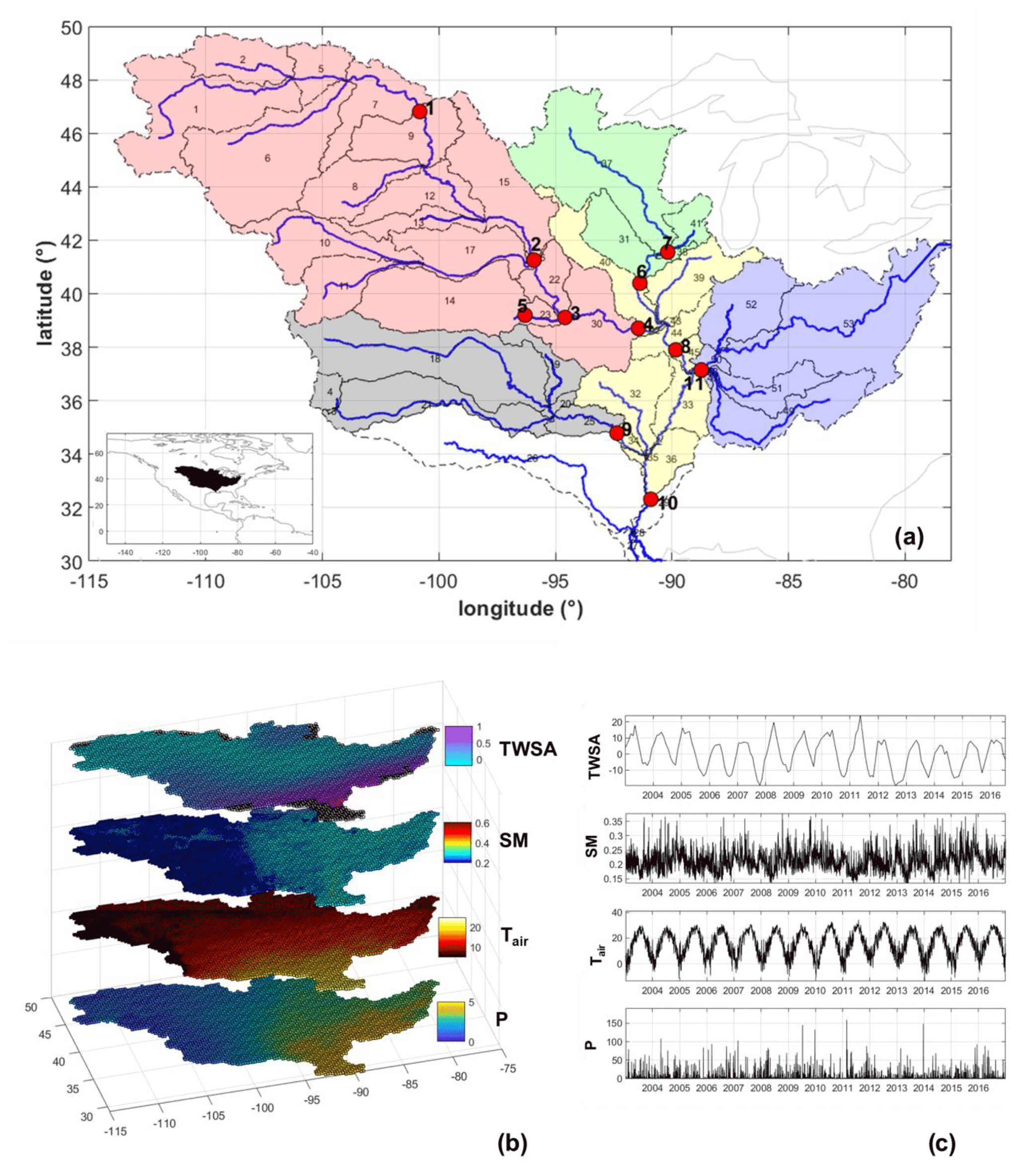
Figure 1 Mississippi River basin. Panel (a) illustrates the sub-catchment delineation. The dashed black lines and the numbers in the map identify the 53 sub-catchments (tributary and directly draining areas) in the Mississippi basin; blue lines represent the mainstem of each sub-catchment. Red dots indicate the location of the river discharge gauging stations; different colors identify different inner cross-sections (and the related contributing sub-catchments) used for the model calibration. Panel (b) shows the gridded mean daily values of the input data for the period 2003–2016. Panel (c) illustrates the input time series over a point located inside the basin.

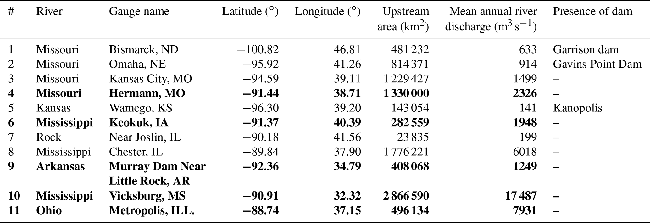
The river flow has a clear natural seasonality that is mainly controlled by spring snowmelt (coming from the Missouri and Upper Mississippi rivers, the western and north-central part of the basin, respectively; Dyer, 2008) and by heavy precipitation exceeding the soil moisture storage capacity (mostly occurring in the eastern and southern part of the basin; Berghuijs et al., 2016). The basin is also heavily regulated by the presence of large dams (Global Reservoir and Dam Database (GRanD); Lehner et al., 2011), most of them located on the Missouri River and over the Great Plains. In particular, the river reach between Garrison and Gavins Point dams is the portion of the Missouri River where the large main-channel dams have the greatest impact on river discharge, providing a substantial reduction in the annual peak floods, an increase on low flows, and a reduction on the overall variability of intra-annual discharges (Alexander et al., 2012). The annual average of Mississippi River discharge at Vicksburg, the outlet river cross-section of the basin, is equal to 17 500 m³ s⁻¹ (see Table 1). Given the variety of climate and topography across the Mississippi River basin, it is a good candidate to test the suitability of the STREAM model for river discharge and runoff modeling.

Table 1 Location of river discharge gauging stations over the Mississippi basins and contributing upstream area. Bold text is used to indicate gauges where the STREAM model has been calibrated.

3 Datasets

The datasets used in this study include in situ observations, satellite products, and runoff verification data. The first two datasets are used as input data to the STREAM model. Conversely, the runoff verification data are used as a benchmark to validate the performance of the STREAM model in simulating the runoff.

3.1 In situ observations

In situ observations comprise air temperature and river discharge data.

For air temperature data, the Climate Prediction Center's (CPC) global temperature data developed by the American National Oceanic and Atmospheric Administration (NOAA), using the optimal interpolation of quality-controlled gauge records from the Global Telecommunication System (GTS) network (Fan and van den Dool, 2008) have been used. The dataset is available on a global regular $\mathrm{0.5}{}^{\circ }\times \mathrm{0.5}{}^{\circ }$ grid and provides daily maximum (T_max) and minimum (T_min) air temperature data from 1979 to present (2022). The daily average air temperature data have been generated as the mean of T_max and T_min of each day.

Daily river discharge data over the study basin have been taken from the Global Runoff Data Center (GRDC; https://www.bafg.de/GRDC/EN/Home/homepage_node.html, last access: 26 August 2022). In particular, 11 gauging stations located along the main river network of the Mississippi River basin have been selected to represent the spatial distribution of river discharge over the basin. The location of these gauging stations along with relevant characteristics (e.g., the upstream basin area, the mean annual river discharge, and the presence of upstream dams) are summarized in Table 1. Mean annual river discharge ranges from 141 to 17 500 m³ s⁻¹, and 3 of 11 gauges are located downstream of big dams (Lehner et al., 2011). In particular, gauges 1, 2, and 5 are located downstream of Garrison (the fifth-largest earthen dam in the world), Gavins Point and Kanopolis dams, respectively (see Fig. 1a and Table 1). The related reservoirs have a maximum storage of 29.383×10⁹, 0.607×10⁹, and 1.058×10⁹ m³, respectively.

3.2 Satellite products

Satellite products include observations of precipitation, soil moisture, and TWSA.

The satellite precipitation dataset used in this study is the TMPA 3B42 Version 7 (hereafter referred to as TMPA) estimate produced by the National Aeronautics and Space Administration (NASA) as the $\mathrm{0.25}{}^{\circ }\times \mathrm{0.25}{}^{\circ }$ quasi-global (50^∘ S–50^∘ N) gridded dataset. The TMPA is a gauge-corrected satellite product, with a latency period of 2 months, available at 3 h sampling interval from 1998 to 2022. Major details about the P dataset, downloadable from http://pmm.nasa.gov/data-access/downloads/trmm (last access: 26 August 2022), can be found in Huffman et al. (2007).

Soil moisture data have been taken from the European Space Agency's Climate Change Initiative (ESA CCI) soil moisture project (https://esa-soilmoisture-cci.org/, last access: 26 August 2022) that provides a surface soil moisture product (referred to first 2–3 cm of soil) continuously updated in terms of spatiotemporal coverage, sensors, and retrieval algorithms (Dorigo et al., 2017). In this study, the daily combined ESA CCI soil moisture product v4.2 is used. It is available at global scale with a grid spacing of 0.25^∘, for the period 1978 to 2022.

The TWSA data have been obtained from the GRACE satellite mission. Here we employ the NASA Goddard Space Flight Center (GSFC) global mascon model, i.e., release v02.4 (Luthcke et al., 2013). It has been produced based on the mass concentration (mascon) approach. The model provides surface mass densities on a monthly basis. Each monthly solution represents the average of surface mass densities within the month, referenced at the middle of the corresponding month. The model has been developed directly from GRACE level-1b K-Band Ranging (KBR) data. It is computed and delivered as surface mass densities per patch over blocks of approximately $\mathrm{1}{}^{\circ }\times \mathrm{1}{}^{\circ }$ or about 12 000 km². Although the mascon size is smaller than the general spatial resolution of GRACE of about 160 000 km², the model exhibits a relatively high spatial resolution. This is attributed to a statistically optimal Wiener filtering, which uses signal and noise full covariance matrices. This allows the filter to fine tune the smoothing in line with the signal-to-noise ratio (SNR) in different areas. That is, the less smoothing, the higher SNR in a particular area and vice versa. This ensures that the filtering is minimal and aggressive smoothing is avoided when unnecessary. Further details of such a filter can be found in Klees et al. (2008). Importantly, the colored noise characteristic of KBR data was taken into account when compiling the GRACE model, which has allowed for a reliable computation of the aforementioned full noise covariance matrices. They play a crucial role when filtering and allow a higher spatial resolution compared to commonly applied GRACE filtering methods, such as Gaussian smoothing and/or destriping filters. The GRACE data used here are available from January 2003 to July 2016, which suffices to demonstrate the STREAM capabilities. With its successor mission GRACE-FO, launched early 2018, the time series of time-variable gravity has reached a nearly uninterrupted time span of about 20 years, thus allowing a continued and operational use of STREAM. The existing interruptions, short ones due to mission operations or technical failures, but also the 1-year gap between GRACE and GRACE-FO, can be dealt with in various ways, e.g., by data-driven gap filling (Yi and Sneeuw, 2021).

3.3 Runoff verification data

To establish the quality of the STREAM model in runoff simulation, monthly runoff data obtained from the Global Runoff Reconstruction (GRUN_v1, https://doi.org/10.3929/ethz-b-000324386, Ghiggi et al., 2019b) have been used for comparison. The GRUN dataset (Ghiggi et al., 2019a) is a global monthly runoff dataset derived through the use of a machine-learning algorithm trained with in situ river discharge observations of relatively small catchments (<2500 km²) and gridded precipitation and temperature derived from the Global Soil Wetness Project Phase 3 (GSWP3) dataset (Kim et al., 2017). The dataset covers the period from 1902 to 2014 and is provided on a $\mathrm{0.5}{}^{\circ }\times \mathrm{0.5}{}^{\circ }$ regular grid.

4 Method

4.1 STREAM model: the concept

The STREAM model conceives river discharge as a combination of hydrological responses operating at diverse timescales (Blöschl et al., 2013; Rakovec et al., 2016). In particular, river discharge can be considered made up of a slow-flow component, produced as outflow of the groundwater storage and of a quick-flow component, i.e., mainly related to the surface and shallow-subsurface runoff components (Hu and Li, 2018).

While the high spatiotemporal variability of precipitation and the highly changing spatial distribution of land cover significantly impact the variability of the quick-flow river discharge component (with scales ranging from hours to days and meters to kilometers depending on the basin size), slow-flow river discharge reacts to precipitation inputs more slowly as water infiltrates, it is stored, mixed, and eventually released in times spanning from weeks to months. Therefore, the two components can be estimated by relying upon two different approaches that involve different types of observations. Based on that, within the STREAM model, satellite soil moisture, precipitation and TWSA will be used for deriving river discharge and runoff estimates. The first two variables are used as proxy of the quick-flow river discharge component while TWSA is exploited for obtaining its complementary part, i.e., the slow-flow river discharge component. Firstly, we exploit the role of the soil moisture in determining the response of the catchment to the precipitation inputs, which have been soundly demonstrated in more than 10 years of literature studies (see e.g., Brocca et al., 2017, for a comprehensive discussion on the topic). Secondly, we consider the important role of total water storage in determining the slow-flow river discharge component as modeled in several hydrological models (e.g., Sneeuw et al., 2014).

It is worth noting that modeling the quick-flow and slow-flow river discharge components independently has been largely applied and tested in recent and past studies, e.g., for the estimation of the flow duration curve (see e.g, Botter et al., 2007a, b; Yokoo and Sivapalan, 2011; Muneepeerakul et al., 2010; Ghotbi et al., 2020).

4.2 STREAM model

The STREAM model is a semi-distributed conceptual hydrological model that uses gridded satellite-derived inputs of precipitation, soil moisture, TWSA, and air temperature to estimate daily values of gridded runoff and river discharge time series at select basin outlets.

To set up the model, the catchment is divided into b sub-catchments, each one representing either a tributary draining area with outlet along the main channel or an area draining directly into the main channel (see Fig. 2). Each sub-catchment, assumed homogeneous, is further divided into an array N_b of individual cells assumed as the unit basis for the runoff generation. Note that the number N_b differs for each sub-catchment since, for a fixed grid-cell size, it varies with the sub-catchment area. Once estimated at cell scale and aggregated at the sub-basin scale (see Sect. 4.2.1 for details), the runoff is routed at each sub-catchment outlet (see Sect. 4.2.2) and then transferred through the channels and the rivers for the computation of the river discharge at intermediate outlets or at the outlet of the entire basin (see Sect. 4.2.3).

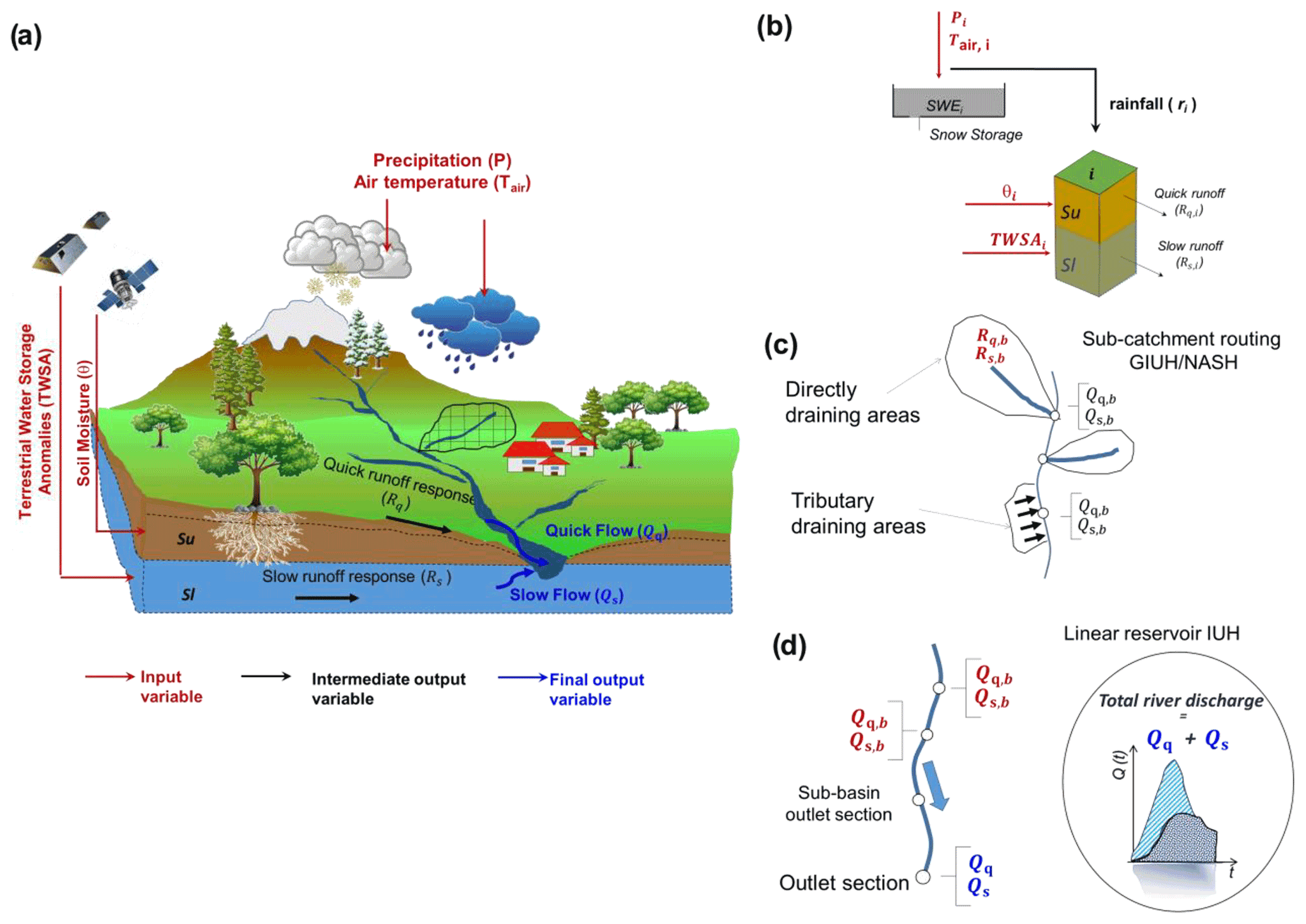
Figure 2 Configuration of the STREAM model adopted for runoff and river discharge estimation. Panel (a) gives an overview of the needed input data and the variables can be obtained as model output. Panel (b) illustrates the runoff generation at cell scale. Panel (c) refers to the sub-catchment river discharge calculation and panel (d) illustrates the river discharge routing through river networks. Red arrows indicate input variables; black arrows indicate intermediate output variables; blue arrows indicate final output variables. Please refer to text for symbols.

Based on that, hereinafter we refer to river discharge, Q, to indicate the amount of water passing a particular point of a river (in m³ s⁻¹), whereas runoff, R, is regarded as the depth of water produced from a drainage area during a particular time interval (in mm). The difference between the two quantities is related to the routing processes that allow runoff to transform into river discharge.

4.2.1 Runoff generation at cell scale

The soil zone of each cell i of the basin is divided into two layers, i.e., the upper and lower soil storages, allowing it to model the related runoff responses, R_q,i [mm] and R_s,i [mm], as illustrated in Fig. 2b.

The upper cell storage receives inputs from precipitation (P_i), released through a snow module (Cislaghi et al., 2020) as rainfall (r_i), or stored as snow water equivalent (SWE_i) within the snowpack and on the glaciers. In particular, according to Cislaghi et al. (2020), SWE_i is modeled by using air temperature (T_air,i) as input and a degree-day coefficient, C_m, to be estimated by calibration.

Once precipitation is partitioned by the snow model, the rainfall output r_i contributes to R_q,i while the SWE_i (like other fluxes contributing to modify the soil water content into Su) is neglected as already considered in the satellite TWSA. Therefore, the first key point of the STREAM model is that the water content in the upper storage of soil zone, Su (Fig. 2b), is directly provided by the satellite observations of soil moisture, and the loss processes like percolation or evaporation do not need to be explicitly modeled to estimate the evolution in time of soil moisture. Consequently, for each cell i, R_q,i can be computed following the formulation proposed by Georgakakos and Baumer (1996), as in Eq. (1):

$$\begin{array}{}\text{(1)}& R_{\mathrm{q},i}\left(t\right)=r_i\left(t\right){\text{SWI}}_i(t,T{)}^{\mathit{\alpha }},\end{array}$$

where t [d] denotes the time; r_i [mm] is the rainfall, obtained as an output from the snow module; SWI_i [–] is the Soil Water Index (Wagner et al., 1999), i.e., the root-zone soil moisture product referred to as the first layer of the model (representative of the first 5–30 cm of soil), derived by the surface satellite soil moisture product, θ_i, by applying the exponential filtering approach in its recursive formulation (Albergel et al., 2009):

$$\begin{array}{}\text{(2)}& {\text{SWI}}_{i,n}={\text{SWI}}_{i,n-\mathrm{1}}+K_n\left({\mathit{\theta }}_i\right(t_n)-{\text{SWI}}_{i,n-\mathrm{1}}),\end{array}$$

where the gain K_n at the time t_n is given by

$$\begin{array}{}\text{(3)}& K_n={\displaystyle \frac{K_{n-\mathrm{1}}}{K_{n-\mathrm{1}}+e^{\left(\frac{t_n-t_{n-\mathrm{1}}}{T}\right)}}},\end{array}$$

where T [d] is a parameter, named characteristic time length, that characterizes the temporal variation of soil moisture within the root-zone profile and the gain K_n ranges between 0 and 1; α [–] is a coefficient linked to the non-linearity of the infiltration process and it considers the characteristics of the soil; for the initialization of the filter K₁=1 and SWI₁=θ(t₁).

The second key point of the STREAM model concerns the estimation of R_s,i, i.e., the slow-runoff response related to the lower storage of the soil zone. The hypothesis here, shared also with other studies (e.g., Rakovec et al., 2016), is that the dynamic of R_s can be represented by the monthly TWSA data. Indeed, the timescale of R_s is typically in the range of seasons to years and it can be assumed almost independent of the water that is contained in the upper storage. For that reason, for each cell i, R_s,i can be computed following the formulation proposed by Famiglietti and Wood (1994), through Eq. (4) as follows:

$$\begin{array}{}\text{(4)}& R_{\mathrm{s},i}\left(t\right)=\mathit{\beta }\left({\text{TWSA}}_i^{\ast }\right(t){)}^m,\end{array}$$

where ${\text{TWSA}}_i^{\ast }$ [–] is the TWSA estimated by GRACE over the cell i, normalized by its minimum and maximum values. The assumption underlying this equation is that TWSA can be assumed as a proxy of the evolution in time of the Sl, i.e., the water amount in the lower storage of the soil zone. The two parameters describing the nonlinearity between lower storage runoff component and TWSA^∗ are β [mm h⁻¹] and m [–].

Note that we formulated the hypothesis that observations of soil moisture and TWSA are independent (whereas in reality soil moisture can be responsible for both the generation of R_q (mainly) and the contribution of R_s), given the different temporal (and spatial) scales at which the upper and lower runoff responses act.

By neglecting any lateral flow, the runoff responses at cell scale are averaged at sub-catchment scale to obtain b runoff responses, one for each sub-catchment. Specifically, by considering N_b cells for each sub-catchment, the following equations are used:

$$\begin{array}{}\text{(5)}& {\displaystyle }{R}_{\mathrm{q},b}\left(t\right)={\displaystyle \frac{{\sum }_{i=\mathrm{1}}^{N_b}{R}_{\mathrm{q},i}\left(t\right)}{N_b}},\text{(6)}& {\displaystyle }{R}_{\mathrm{s},b}\left(t\right)={\displaystyle \frac{{\sum }_{i=\mathrm{1}}^{N_b}{R}_{\mathrm{s},i}\left(t\right)}{N_b}}.\end{array}$$

4.2.2 Sub-catchment river discharge calculation

For each sub-catchment b, the runoff component R_q,b is routed to its outlet by the geomorphological instantaneous unit hydrograph (GIUH; Gupta et al., 1980) for tributary draining areas or through a linear reservoir approach (Nash, 1957) for directly draining areas. The R_s,b runoff component is transferred to the sub-catchment outlet by a linear reservoir approach. These processes are controlled by a parameter lag time, L [d], evaluated as (Corradini et al., 2002):

$$\begin{array}{}\text{(7)}& L=\mathit{\gamma }\mathrm{1.19}{A}_b^{\mathrm{0.33}},\end{array}$$

where A_b [km²] is the sub-catchment area and γ [–] is a parameter to be calibrated.

By routing the R_q,b and R_s,b components, the quick-flow, Q_q,b [m³ s⁻¹], and the slow-flow, Q_s,b [m³ s⁻¹], river discharge components at each sub-catchment outlet are obtained (see Fig. 2c).

4.2.3 River discharge routing through river networks

A diffusive linear approach (controlled by the parameters C [km h⁻¹] and D [km² h⁻¹], i.e., celerity and diffusivity, Troutman and Karlinger, 1985) is applied to route the two river discharge components, Q_q,b and Q_s,b through the river network from the sub-catchment outlet to intermediate outlets along the river or to the outlet of the entire basin (Brocca et al., 2011). In this way the quick-flow, Q_q [m³ s⁻¹], and the slow-flow, Q_s [m³ s⁻¹], river discharge components at the catchment outlet are obtained (see Fig. 2d).

4.3 STREAM parameters

The STREAM model uses eight calibration parameters for each sub-catchment b into which the entire basin is divided. Among these parameters, five control the runoff generation process (α, T, β, m, C_m) and 3 the routing component, and therefore the streamflow dynamics (γ, C and D). The parameter values determined within the feasible parameter space (see Table A1 for more details), are calibrated by maximizing the Kling–Gupta efficiency (KGE) index (Gupta et al., 2009; Kling et al., 2012, see Sect. 5.1 for more details) between observed and modeled river discharge. For model calibration, a standard gradient-based automatic optimization method (Bober, 2013) was used.

5 Experimental design

5.1 Modeling setup for Mississippi River basin

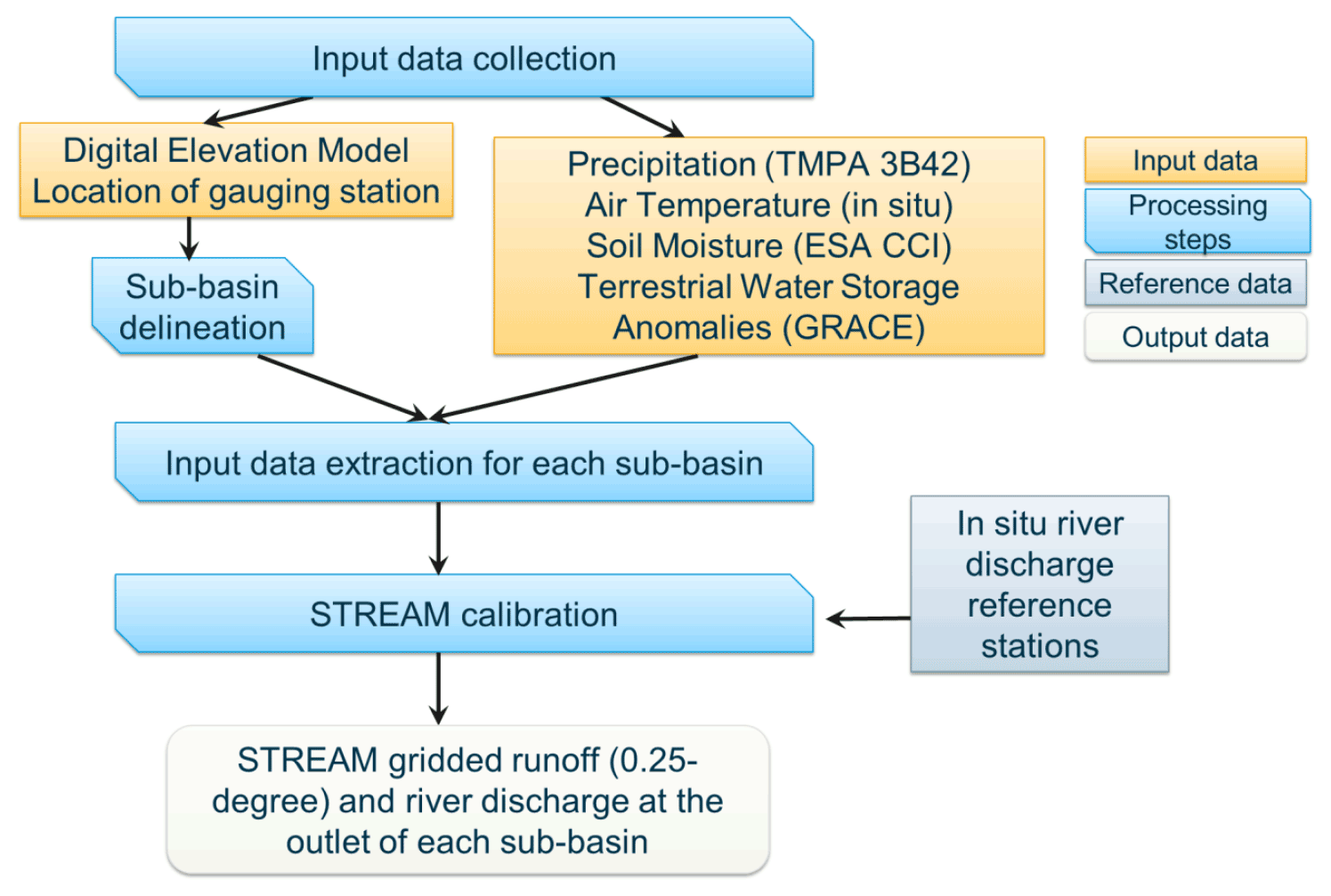
The modeling setup is carried out in three steps (Fig. 3):

Figure 3 Processing steps of the STREAM model.

1. Sub-catchment delineation. The TopoToolbox (https://topotoolbox.wordpress.com/, last access: 26 August 2022), a tool developed in MATLAB by Schwanghart and Kuhn (2010), and the SHuttle Elevation Derivatives at multiple Scales (HydroSHED, https://www.hydrosheds.org/, last access: 26 August 2022) DEM of the basin at 3 arcsec resolution (nearly 90 m at the Equator) have been used to derive flow directions, to extract the stream network, and to delineate the drainage basins over the Mississippi River basin. In particular, by only considering rivers with an order greater than 3 (according to the Horton–Strahler rules, Horton, 1945; Strahler, 1952), the Mississippi watershed has been divided into 53 sub-catchments as illustrated in Fig. 1a. Blue lines in the figure illustrate the river network pathway connecting the sub-catchments, red dots indicate the location of the 11 river discharge gauging stations selected for the study area.

   It has to be specified that the step of sub-basin delineation could be accomplished through tools different from the TopoToolbox. For instance, the free QGIS software downloadable at https://www.qgis.org/it/site/forusers/download.html (last access: 26 August 2022)could be used, following the instruction to perform the hydrological analysis as in https://docs.qgis.org/3.16/en/docs/training_manual/processing/hydro.html?highlight=hydrological%20analysis (last access: 26 August 2022).

2. Extraction of input data. Precipitation, air temperature, soil moisture, and TWSA datasets data have to be extracted for each sub-catchment of the study area. If characterized by different spatial/temporal resolution, these datasets need to be resampled over a common spatial grid/temporal time step prior to being used as input into the model.

   To run the STREAM model over the Mississippi River basin, input data have been resampled over the precipitation spatial grid at 0.25^∘ resolution through a bilinear interpolation. Concerning the temporal scale, air temperature, soil moisture, and precipitation data are available at daily time steps, while monthly TWSA data have been linearly interpolated at daily time steps. For each of the 53 Mississippi sub-catchments, the resampled precipitation, soil moisture, air temperature, and TWSA data have been extracted (see Fig. 1b and c).

3. STREAM model calibration. In situ river discharge data are used as reference data for the calibration of STREAM model. For Mississippi, the STREAM model has been calibrated at five gauging stations, i.e., the stations 4, 6, 9, 10, and 11. This allowed us to identify five sets of STREAM parameters attributed to each catchment according to the river network pathway illustrated in Fig. 1a. This means that, for example, the sub-catchments labeled as 1, 2, and 5 to 15, 17, 22, 23, and 30 contributing to the gauging station 4, are attributed to the parameter set obtained by calibrating the model against river discharge data observed at station 4; the sub-catchments 31, 37, 38 and 41 contributing to gauging station 6 are attributed to the parameter set obtained by calibrating the model with respect to gauging station 6, and so on. Consequently, the sub-catchments highlighted with the same color in Fig. 1a are assigned the same model parameters, i.e., the parameters that allow us to reproduce the river discharge data observed at the related gage.

   Once calibrated, the STREAM model has been run to provide continuous daily runoff and river discharge time series, over each grid pixel and at the outlet section of each sub-catchment, respectively. By considering the spatial/temporal availability of both in situ and satellite observations, the entire analysis period covers the maximum common observation period, i.e., from January 2003 to July 2016 at daily timescales. To establish the goodness-of-fit of the model, the modeled river discharge and runoff time series are compared against in situ river discharge and modeled runoff data.

5.2 Model evaluation criteria and performance metrics

The model has been run over a 13.5-year period split into two sub-periods: the first 8 years (January 2003–December 2010) are used to calibrate the model. The model is validated, as described below, over the remaining 5.5 years (January 2011–July 2016).

In particular, three different validation schemes have been adopted to assess the robustness of the STREAM model:

1. internal validation aimed to test the plausibility of both the model structure and the parameter set in providing reliable estimates of the hydrological variables against which the model is calibrated. For this purpose, a comparison between observed and modeled river discharge time series on the gauging stations used for model calibration has been carried out for both the calibration and validation sub-periods;

2. cross-validation testing the goodness of the model structure and the calibrated model parameters to predict hydrological variables at locations not considered in the calibration phase. In this respect, the cross-validation has been carried out by comparing observed and modeled river discharge time series in gauging stations not considered during the calibration phase;

3. external validation aimed at testing the capability of the model “to get the right answers for the right reasons” (Kirchner, 2006). The rationale behind this concept is that today the hydrological models are high-performing and able to reproduce a lot of hydrological variables. For that reason, the model performances should be evaluated against not only observed river discharge, but also complementary datasets representing internal hydrologic states and fluxes (e.g., soil moisture, evapotranspiration, runoff). As runoff is a secondary product of the STREAM model, obtained indirectly from the calibration of the river discharge (basin-integrated runoff), the comparison in terms of runoff can be considered as a further external validation of the model. Runoff, different from river discharge, cannot be measured directly. It is generally modeled through land surface or hydrological models. Its validation requires a comparison against modeled data that suffer from uncertainties (Beck et al., 2017). Based on that, the GRUN runoff dataset described in Sect. 3.3 has been used in this study for a qualitative comparison.

5.3 Performance metrics

To measure the goodness-of-fit between modeled and observed river discharge data, three performance scores have been used:

• the root mean square error relative to the mean, rRMSE:

  $$\begin{array}{}\text{(8)}& \text{rRMSE}={\displaystyle \frac{\sqrt{\frac{\mathrm{1}}{n}{\sum }_{j=\mathrm{1}}^n(Q_{{\text{mod}}_j}-Q_{{\text{obs}}_j}{)}^{\mathrm{2}}}}{\frac{\mathrm{1}}{n}{\sum }_{j=\mathrm{1}}^n\left(Q_{{\text{obs}}_j}\right)}},\end{array}$$

  where Q_obs and Q_mod are the observed and modeled river discharge time series of length n. The rRMSE values range from 0 to +∞; the lower the rRMSE, the better the agreement between observed and modeled data.

• the Pearson correlation coefficient, rho, measuring the linear relationship between two variables:

  $$\begin{array}{}\text{(9)}& \text{rho}={\displaystyle \frac{{\sum }_{j=\mathrm{1}}^n(Q_{{\text{mod}}_j}-\stackrel{\mathrm{‾}}{Q_{\text{mod}}})(Q_{{\text{obs}}_j}-\stackrel{\mathrm{‾}}{Q_{\text{obs}}})}{\sqrt{{\sum }_{j=\mathrm{1}}^n(Q_{{\text{mod}}_i}-\stackrel{\mathrm{‾}}{Q_{\text{mod}}}{)}^{\mathrm{2}}(Q_{{\text{obs}}_j}-\stackrel{\mathrm{‾}}{Q_{\text{obs}}}{)}^{\mathrm{2}}}}},\end{array}$$

  where $\stackrel{\mathrm{‾}}{Q_{\text{obs}}}$ and $\stackrel{\mathrm{‾}}{Q_{\text{mod}}}$ represent the mean values of Q_obs and Q_mod, respectively. The values of rho range between −1 and 1; higher values of rho indicate a better agreement between observed and modeled data.

• the KGE index (Gupta et al., 2009), which provides direct assessment of four aspects of river discharge time series, namely shape, timing, water balance, and variability. It is defined as follows:

  $$\begin{array}{}\text{(10)}& \text{KGE}=\mathrm{1}-\sqrt{(\text{rho}-\mathrm{1}{)}^{\mathrm{2}}+(\mathit{\delta }-\mathrm{1}{)}^{\mathrm{2}}+(\mathit{\epsilon }-\mathrm{1}{)}^{\mathrm{2}}},\end{array}$$

  where δ is the relative variability and ε the bias normalized by the standard deviation between observed and modeled river discharge. The KGE values range between −∞ and 1; the higher the KGE the better the agreement is between observed and modeled data. Simulations characterized by values of KGE in the range of −0.41 and 1 can be assumed to be reliable; values of KGE greater than 0.5 have been assumed to be good with respect to their ability to reproduce observed time series (Thiemig et al., 2013).

5.4 STREAM sensitivity analysis

To investigate how the variation of the STREAM parameters influences the variation of the STREAM model outputs, a global sensitivity analysis has been carried out. Specifically, the variance-based sensitivity analysis (VBSA; Sobol, 1993) implemented into the Sensitivity Analysis For Everybody (SAFE) toolbox (Pianosi et al., 2015, https://www.safetoolbox.info/, last access: 26 August 2022) has been applied. The VBSA relies on the variance decomposition and consists of assessing the contributions to the variance of the model output from variations in the parameters. In this study, we use as sensitivity index the first-order (main effect) index, which measures the variance contribution from variations in an individual input factor alone (i.e., excluding interactions with other factors), and the total sensitivity indices, which measure the total contribution of a single input factor or a group of inputs including interactions with all other inputs. The following steps were carried out to perform the VBSA. Firstly, the locality-sensitive hashing (LSH) technique was used to generate 15 000 samples from the model parameter space (see Table A1). Previous hydrological studies (e.g., Tang et al., 2007) recommend the LHS sampling method for its sampling efficiency. Secondly, 15 000 STREAM model runs were executed and the corresponding KGE values (11×15 000 values, one for each gauging station for each run) were retained. Thirdly, the parameters and the 15 000 KGE samples were used in the SAFE toolbox to compute the sensitivity indices.

For major details on the workflow needed to implement the VBSA, the reader is referred to Noacco et al. (2019).

6 Results

The testing and validation of the STREAM model is presented and discussed in this section according to the scheme illustrated in Sect. 5.2.

6.1 Internal validation

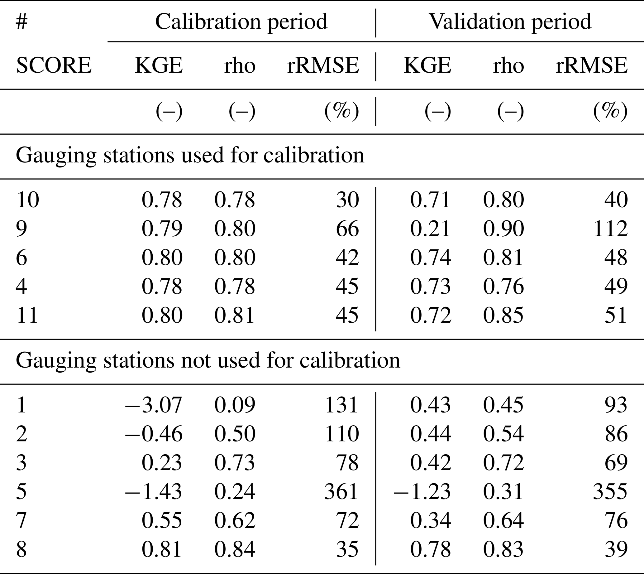
The performance of the STREAM model over the gauging stations used for calibration is illustrated in Fig. 4 and summarized in Table 2. Figure 4 shows observed and modeled river discharge time series over the whole study period (2003–2016); in Table 2 the performance scores are evaluated separately for the calibration and validation sub-periods. It is worth noting that the model accurately predicts the observed river discharge data and is able to give the “right answer” with good modeling performances. Score values of KGE and rho over the calibration period are higher than 0.78 for all the calibrated gauging stations; rRMSE is lower than 45 % for all the calibrated gauging stations except for station 9, where it rises up to 66 %. The performances remain good even if they are evaluated over the validation period or the entire study period, as indicated by the scores at the top of each plot of Fig. 4.

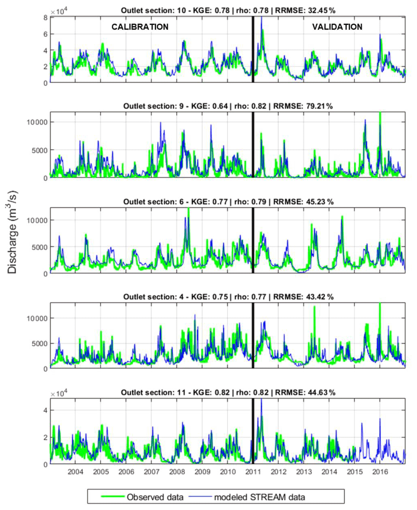
Figure 4 Comparison between observed and modeled river discharge time series over the five calibrated sections in the Mississippi River basin. Performance scores at the top of each plot refer to the entire study period (2003–2016).

Table 2 Performance scores obtained over the Mississippi River gauging stations during the calibration and validation periods.

6.2 Cross-validation

The cross-validation has been carried out over the six gauging stations illustrated in Fig. 5 that were not used in the calibration step. The performance scores at the top of each plot refer to the entire study period; the scores split for calibration and validation periods are reported in Table 2. For some river discharge gauging stations the performance is quite low (see, e.g., gauging station 1, 2 and 5), whereas for others the model is able to estimate river discharge data quite accurately (e.g., 7 and 8). In particular, for the gauging stations 1 and 2, even if KGE reaches values equal to 0.39 and 0.46 for the entire period, respectively, there is not a good agreement between observed and modeled river discharge and the rho score is lower than 0.56 for both stations. The worst performance is obtained over the gauging station 5, with negative KGE and low rho values. These results are certainly influenced by the presence of large dams located upstream of these stations (i.e., Garrison, Gavins Point, and Kanopolis dams, see Table 1) which have a strong impact on river discharge: the model, not having a specific module for modeling reservoirs, is not able to accurately reproduce the dynamics of river discharge over regulated river stations. Positive KGE values are obtained over the gauging stations 3, 7, and 8. In particular, over the gauging station 3 the STREAM model overestimates the observed river discharge due to the presence of large dams along the Missouri River, over the Great Plains region. This area is well known from other large-scale hydrological models (e.g., ParFlow-CLM and WRF-Hydro) to be an area with very low performances in terms of river discharge modeling (O'Neill et al., 2021; Tijerina et al., 2021).

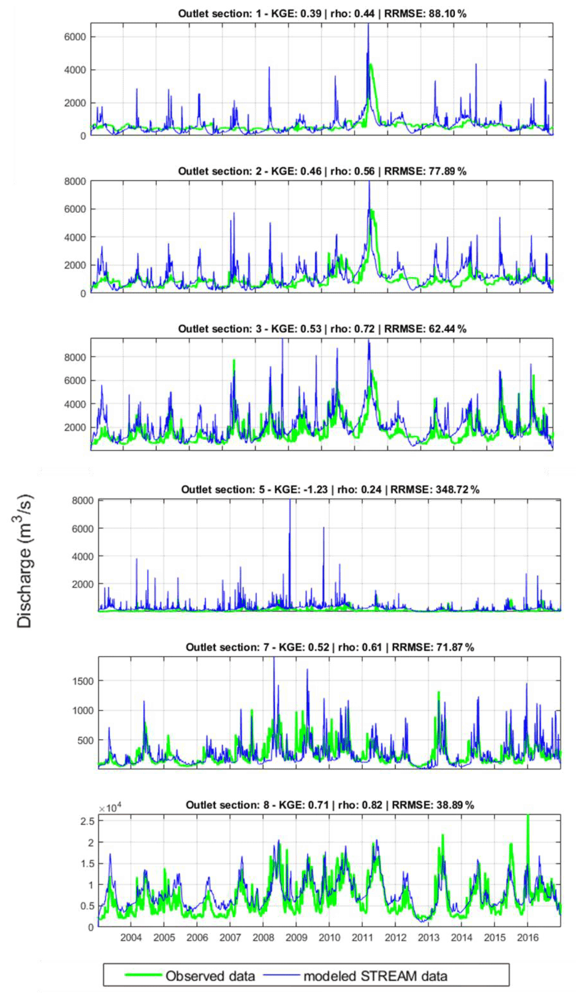
Figure 5 Comparison between observed and modeled river discharge time series over the gauged sections not used in the calibration phase. Performance scores at the top of each plot refer to the entire study period (2003–2016).

Over the gauging station 7 located over the Rock River, a relatively small tributary of the Mississippi River (see Table 1), the STREAM model overestimation has to be attributed to (1) the different characteristics of the Rock River basin regarding the entire basin, close to station 6 where the model has been calibrated (see Fig. 1a); (2) the small size of the Rock River basin (23 000 km², if compared with the GRACE resolution, 160 000 km²) for which the model accuracy is expected to be lower. Conversely, the performances over the gauging station 8, whose parameters have been set equal to the ones of gauging station 10, are quite high (KGE equal to 0.71, 0.81, and 0.78 for the entire, calibration, and validation periods, respectively; rho equal to 0.82, 0.84, and 0.83 for the entire, calibration and validation periods, respectively). This outcome demonstrates that under some circumstances, the STREAM model can be used to estimate river discharge in basins not calibrated, especially those without upstream dams and with comparable size and land cover.

Overall, the cross-validation results suggest that the performances of the STREAM model, as any hydrological model calibrated against observed data, decrease over the gauging stations not used for the calibration, raising doubts about the robustness of model parameters and whether it is actually possible to transfer model parameters from one river section to another with different inter-basin characteristics. A more in-depth investigation about the model calibration procedure, with special focus on the regionalization of the model parameters, should be conducted, but this topic is beyond the scope of this paper.

6.3 External validation

For the external validation, the monthly runoff time series provided by the GRUN dataset have been compared against the ones computed by the STREAM model. For that reason, the STREAM daily runoff time series have been aggregated at monthly scales and re-gridded at the same spatial resolution of the GRUN dataset (0.5^∘). The comparison is illustrated in Fig. 6 for the common period 2003–2014. Although the two datasets consider different precipitation inputs, the two models agree in identifying two distinct zones in terms of runoff, i.e., the western dry and the eastern wet area. These two distinct zones can also be clearly identified in the GSWP3 and TMPA 3B42 V7 precipitation maps (see Fig. A1) used as input in GRUN and STREAM, respectively, emphasizing that the STREAM runoff output is correctly driven by the input data. However, likely due to the calibration procedure, the STREAM runoff map appears patchier with respect to GRUN, and discontinuities along the sub-basin boundaries (identified in Fig. 1a) can be noted. This should be ascribed to the automatic calibration procedure of the model that, different from other calibration techniques (e.g., regionalization procedures), does not consider the basin's physical attributes like soil, vegetation, and geological properties that govern spatial dynamics of hydrological processes. This calibration procedure can generate sharp discontinuities, even for neighboring sub-catchments that are calibrated individually. It leads to discontinuities in model parameter values and consequently in the modeled hydrological variable (runoff).

Figure 6 Mississippi River basin: mean monthly runoff for the period 2003–2014 obtained by STREAM and GRUN models.

6.4 Sensitivity analysis results

The results of the VBSA method are illustrated in Fig. 7a in terms of the main effect indices and in Fig. 7b in terms of total effect. Specifically, the figure refers to Vicksburg station, but similar results have been obtained for all 11 gauging stations in the Mississippi basin. By looking at Fig. 7, we observe that the model parameters influencing the model response the most are β and m, i.e., the two parameters controlling the slow-flow runoff response of the lower soil storage. In particular, the total effect sensitivity index of these two parameters is higher than the main effect sensitivity index. This means that these two parameters have an effect on the model output, through not only their individual variations but also interactions with other parameters. Instead, the other six parameters (α, T, γ, C, D and C_m) have low main and total effect indices, and consequently, these parameters have a small effect, both directly and through interactions, on model response. Among these, only the α parameter shows slightly high main and total effect sensitivity indices.

Figure 7 Main effect (a) and total effect (b) sensitivity indices calculated using the VBSA method for Vicksburg gauging station. The boxes represent the 25th and 75th percentiles, and the central black lines indicate the median.

This outcome is very important as it allows us to clearly distinguish model parameters, whose values should be carefully determined when calibrating the model (β and m and partially α), from the least sensitive (T, γ, C, D, and C_m), whose values could be set values within the model parameters' range of variability and then excluded during the calibration phase.

7 Discussion

In the previous sections, the ability of the STREAM model to estimate river discharge and runoff time series has been presented. In particular, Figs. 4–6 demonstrate that satellite observations of precipitation, soil moisture, and TWSAs can provide accurate daily river discharge estimates for near-natural large basins (absence of upstream dams), and for basins with a draining area greater than 160 000 km² (see Sect. 6.2), i.e., at spatial/temporal resolution greater than the ones of the TWSA input data (monthly, 160 000 km²). This is an important result of the study as it demonstrates, on one hand, that the model structure is appropriate with respect to the data used as input and, on the other hand, the great value of information contained in TWSA data that, even if characterized by limited spatial/temporal resolution, can be used to estimate runoff and river discharge at basin scale. This finding has also been confirmed by a preliminary sensitivity analysis in which the STREAM model has been run with different hydrological inputs of precipitation, soil moisture, and TWSA (not shown here for brevity). In particular, by running the STREAM model with different input configurations (e.g., by using TMPA 3B42 V7 or CPC data for precipitation, ESA CCI or Advanced SCATterometer (ASCAT) data for soil moisture, TWSA or ESA CCI soil moisture data to model the slow-flow river discharge component), we found that STREAM results are more sensitive to soil moisture data than to precipitation input. In addition, by running STREAM model with soil moisture data as input to model the slow-flow river discharge component (i.e., without using TWSA data), we found a deterioration in the model results. This outcome along with the one obtained in the Sect. 6.3, demonstrating the high sensitivity of the model parameters related to the slow-flow river discharge component, confirm the paramount role of TWSA in estimating river discharge. In this respect, the availability of GRACE data up to July 2016 could present an issue for the model application beyond that date. However, the GRACE-FO along with the numerous literature studies devoted to fill the GRACE data gap between GRACE and GRACE-FO (see e.g., Landerer et al., 2020, or Yi and Sneeuw, 2021), can provide the needed data to extend the STREAM model application up to 2022. Further developments in this direction are expected with the ESA's Next Generation Gravity Mission (NGGM), a candidate Mission of Opportunity for ESA–NASA cooperation in the frame of the Mass Change and Geosciences International Constellation (MAGIC) that will enable long-term monitoring of the temporal variations of Earth's gravity field at relatively high temporal (down to 3 d) and increased spatial resolutions (up to 100 km). This also implies that time series of GRACE and GRACE-FO can be extended towards a climate series (Massotti et al., 2021).

By looking at technical reviews of large-scale hydrological models (e.g., Sood and Smakhtin, 2015; Kauffeldt et al., 2016), it can be noted that there are many established models, similar in objective and limitations to the STREAM model, already existing with support and user base (e.g., among others, the Community Land Model (CLM), Oleson et al., 2013; European Hydrological Predictions for the Environment (E-HYPE), Lindström et al., 2010; H08, Hanasaki et al., 2008; PCR-GLOBWB, van Beek and Bierkens, 2009; Water – a Global Assessment and Prognosis (WaterGAP), Alcamo et al., 2003; ParFlow–CLM, Maxwell et al., 2015; WRF-Hydro, Gochis et al., 2018; Precipitation-Runoff Modeling System (PRMS), Markstrom et al., 2015). Some of them, e.g., ParFlow-CLM, WRF-Hydro or PRMS, have been specifically configured across the continental United States and showed good capability to reproduce observed streamflow data over the Mississippi River basin with decreased performances throughout the Great Plains (O'Neill et al., 2020; Tijerina et al., 2021), which is consistent with the results we obtained with the STREAM model. However, with respect to classical hydrological and land surface models, STREAM is based on a new concept for estimating runoff and river discharge which relies on the almost exclusive use of satellite observations and a simplification of the processes being modeled.

This approach brings several advantages: (1) satellite data implicitly consider the human impact on the water cycle observing some processes, such as irrigation application or groundwater withdrawals, that are affected by large uncertainty in classical hydrological models, (2) the satellite technology grows quickly and hence it is expected that the spatial/temporal resolution and accuracy of satellite products will be improved in the near future (e.g., 1 km resolution from new satellite soil moisture products and NGGM); the STREAM model is able to fully exploit such improvements; (3) the STREAM model only models the most important processes affecting the generation of runoff, and considers only the most important variables as input (precipitation, surface soil moisture, and groundwater storage). In other words, the model does not need to parameterize processes, such as evapotranspiration and percolation, and therefore it is an independent modeling approach for simulating runoff and river discharge that can be also exploited for benchmarking and improving classical land surface and hydrological models.

7.1 Strengths and limitations of STREAM model

Hereinafter, the strengths and the main limitations of the STREAM model are discussed.

Among the strengths of the STREAM model it is worth highlighting the following:

• Simplicity. The STREAM model is structured as follows: (1) it limits the input data required. Only precipitation, air temperature, soil moisture and TWSA data are needed as input whereas LSM/GHMs require many additional inputs such as wind speed, short-wave and long-wave radiation, pressure, and relative humidity; (2) it limits and simplifies the processes to be modeled for runoff and river discharge simulation. Processes like evapotranspiration or percolation, are not modeled, and hence avoid the need to use sophisticated and highly parameterized equations (e.g., Penman–Monteith for evapotranspiration, Allen et al., 1998); (3) it limits the number of parameters (only 8 parameters have to be calibrated), thus simplifying the calibration procedure and potentially reduces the model uncertainties related to the estimation of parameter values.

  In particular, the STREAM model is even simpler than the classical semi-distributed conceptual hydrological models available in literature. As an example, for the comparison we could refer to the Hydrologiska Byråns Vattenbalansavdelning model (HBV; Bergström, 1995) or to the Hydrologic Engineering Center-Hydrologic Modeling System (HEC-HMS; Feldman, 2000). The HBV model counts 14 parameters to be calibrated and needs precipitation, air temperature, and potential evapotranspiration as input data. Similar input data are required for HEC-HMS which counts 23 parameters. Both models use conceptual equations to estimate the soil losses and to model the soil water storage.

• Versatility. The STREAM model is a versatile model suitable for daily runoff and river discharge estimation over sub-basins characterized by different physiographic/climatic characteristics (see e.g., the outcomes obtained for the gauges 9 and 11 located in the driest and wetter part of the Mississippi basin). This aspect is paramount as it gives insight into the potential of the model to be extended at the global scale. Moreover, the model can be adapted easily to ingest input data with spatial/temporal resolution different from the one tested in this study (0.25${}^{\circ }{\mathrm{d}}^{-\mathrm{1}}$). For instance, satellite missions with higher spatial/temporal resolution (e.g., GPM Final Run, ASCAT and NGGM-MAGIC) or near-real time products (e.g., GPM Early Run, EUMETSAT H16, GRACE European Gravity Service for Improved Emergency Management, EGSIEM GRACE data, Jäggi et al., 2019) could be considered.

  Additionally, the STREAM model shows highly flexibility since (1) it can accommodate application domains comprising single or multiple basins of any size; and (2) the sub-catchment delineation procedure can be adapted easily to introduce intermediate outlets along the river in correspondence of gauges with available observed river discharge data, useful for model calibration.

• Low computational cost. Due to its simplicity and the limited number of parameters to be calibrated, the computational effort for the STREAM model is very limited (model runs requiring seconds to minutes). For instance, a run of the STREAM model over the presented case study takes less than 2 s on a machine with 16 GB RAM and 4 Core.

  However, some limitations have to be acknowledged for the current version of the STREAM model:

• Presence of reservoir, diversion, dams or flood plain. As the STREAM model does not explicitly consider the presence of discontinuity elements along the river network (e.g., reservoir, dam, or floodplain), river discharge estimates obtained for gauging stations located downstream of such elements might be inaccurate (see, e.g., gauging stations 1 and 2 in Fig. 5).

• Snow modeling. A potential limitation of the current version of the STREAM model is related to the rain/snow differentiation, based on the degree-day coefficient. A different scheme based on the wet-bulb temperature, for example, as in Integrated Multi-satellitE Retrievals for GPM (IMERG) (Wang et al., 2019; Arabzadeh and Behrangi, 2021), could be investigated in future developments.

• Need of in situ data for model calibration and robustness of model parameters. As discussed in the results section, the parameter values of the STREAM model are set through an automatic calibration procedure aimed at minimizing the differences between modeled and observed river discharge. The main drawbacks of this parameterization technique are a poor predictability of state variables and fluxes at locations and periods not considered in the calibration, and the presence of sharp discontinuities along sub-basin boundaries in state flux and parameter fields (e.g., Merz and Blöschl, 2004). To overcome these issues, several regionalization procedures, for instance as summarized in Cislaghi et al. (2020), could conveniently be applied to transfer model parameters from hydrologically similar catchments to a catchment of interest. In particular, the regionalization of model parameters could allow us to firstly, estimate river discharge and runoff time series over ungauged basins overcoming the need of river discharge data recorded from in situ networks; secondly, estimate the model parameter values through a physically consistent approach, linking them to the characteristics of the basins; and thirdly, solve the problem of discontinuities in the model parameters, to avoid obtaining patchy unrealistic runoff maps. Since this aspect requires additional investigations and is beyond the purpose of this paper, it will not be addressed here.

8 Conclusions

This study presents a new conceptual hydrological model, STREAM, for runoff and river discharge estimation. By using as input satellite data of precipitation, soil moisture and total water storage anomalies, the model has been able to provide accurate daily river discharge and runoff estimates at the outlet river section and the inner river sections and over a $\mathrm{0.25}{}^{\circ }\times \mathrm{0.25}{}^{\circ }$ spatial grid of the Mississippi River basin. In particular, the model is suitable to reproduce:

1. river discharge time series over the calibrated river section with good performances both in calibration and validation periods;

2. river discharge time series over river sections not used for calibration and not located downstream dams or reservoirs;

3. runoff time series with a quite good agreement with respect to the well-established GRUN observational-based dataset used for comparison.

The integration of observations of soil moisture, precipitation, and TWSAs is the first alternative method for river discharge and runoff estimation with respect to classical methods based on the use of TWSA-only (suitable for river basins larger than 160 000 km², monthly time scale) or on classical LSMs (Cai et al., 2014).

Moreover, although simple, the model has demonstrated a great potential to be easily applied over sub-basins with different climatic and topographic characteristics, also suggesting the possibility to extend its application to other basins. In particular, the analysis over basins with high human impact, where the knowledge of the hydrological cycle and the river discharge monitoring is very important, deserves special attention. Indeed, as the STREAM model is directly ingesting observations of soil moisture and total water storage data, it allows the modeler to neglect processes that are implicitly accounted for in the input data. Therefore, human-driven processes (e.g., irrigation, land use change), that are typically very difficult to model due to missing information, and that might have a large impact on the hydrological cycle, and hence on runoff, could be modeled implicitly. The application of the STREAM model on a larger number of basins with different climatic-physiographic characteristics (e.g., including more arid basins, snow-dominated, lots of topography, heavily managed) along with the results from the sensitivity analysis of the model parameters, will allow us to investigate the possibility to regionalize the model parameters and overcome the limitations of the automatic calibration procedure highlighted in the discussion section.

Appendix A

Table A1 Description of STREAM parameters, belonging module, variability range, and unit.

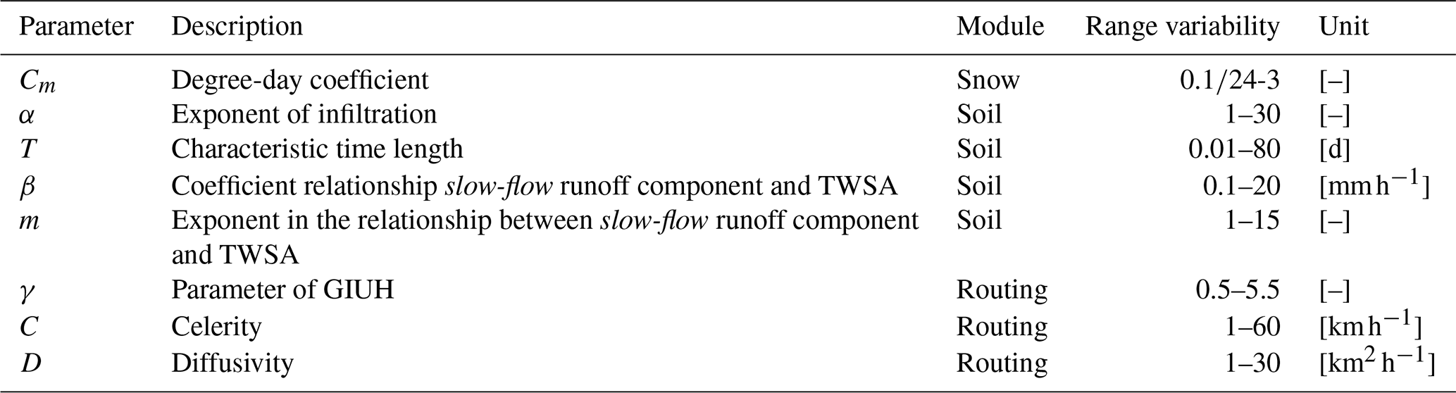
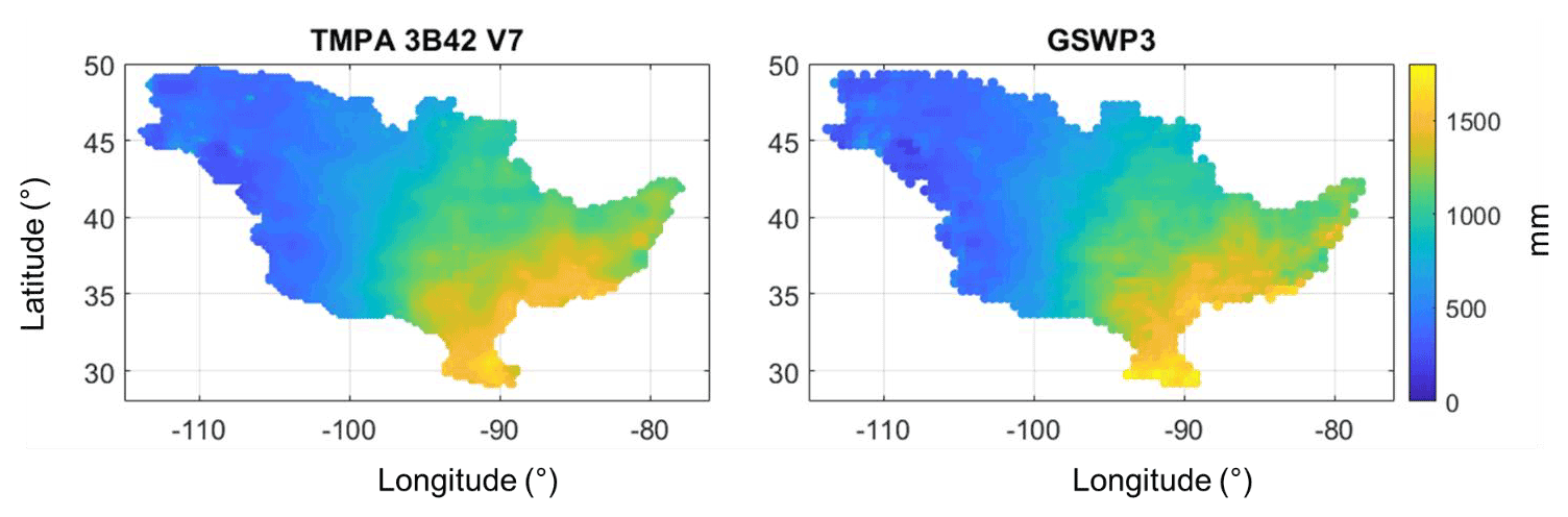
Figure A1 Mean annual precipitation data over the period 2003–2014 obtained by TMPA 3B42 V7 and GSWP3 datasets over the Mississippi River basin.