the Creative Commons Attribution 4.0 License.
the Creative Commons Attribution 4.0 License.
 | 01 Sep 2022
NeverWorld2: an idealized model hierarchy to investigate ocean mesoscale eddies across resolutions
Nora Loose
Elizabeth Yankovsky
Jacob M. Steinberg
Chiung-Yin Chang
Neeraja Bhamidipati
Alistair Adcroft
Baylor Fox-Kemper
Stephen M. Griffies
Robert W. Hallberg
Malte F. Jansen
Hemant Khatri
Laure Zanna
We describe an idealized primitive-equation model for studying mesoscale turbulence and leverage a hierarchy of grid resolutions to make eddy-resolving calculations on the finest grids more affordable. The model has intermediate complexity, incorporating basin-scale geometry with idealized Atlantic and Southern oceans and with non-uniform ocean depth to allow for mesoscale eddy interactions with topography. The model is perfectly adiabatic and spans the Equator and thus fills a gap between quasi-geostrophic models, which cannot span two hemispheres, and idealized general circulation models, which generally include diabatic processes and buoyancy forcing. We show that the model solution is approaching convergence in mean kinetic energy for the ocean mesoscale processes of interest and has a rich range of dynamics with circulation features that emerge only due to resolving mesoscale turbulence.
- Article
(6148 KB) - Full-text XML
- BibTeX
- EndNote


Mesoscale eddies have a profound impact on the transport of properties in the ocean. They affect the currents, stratification, ocean dynamic sea level variability, and uptake of physical and biogeochemical tracers. Eddies thus play an important role in regulating climate on regional and global scales and on timescales of weeks to centuries. Mesoscale eddies form on spatial scales near the baroclinic Rossby deformation radius (Smith and Vallis, 2002; Arbic and Flierl, 2004; Thompson and Young, 2007; Hallberg, 2013). The deformation radius varies regionally between 10–100 km horizontally (Chelton et al., 1998). These scales are too small to be resolved globally in routinely used structured-grid ocean climate simulations and, therefore, must be parameterized.
The most notable scheme of mesoscale eddy transport implemented in climate models is the Gent McWilliams (GM) parameterization, which mimics the effects of baroclinic instability by flattening isopycnals and acting as a net sink of available potential energy (Gent and McWilliams, 1990; Gent et al., 1995). Motivated by the effect on available potential energy, eddy kinetic energy parameterizations have been developed (Cessi, 2008; Eden and Greatbatch, 2008; Marshall and Adcroft, 2010) to keep track of the mechanical energy in idealized simulations (Marshall et al., 2012) and/or scale the GM parameter in global climate simulations (Adcroft et al., 2019). The specific goal of this paper is to present a test for such energy-based parameterizations, although mesoscale parameterizations based on other approaches can also be tested in the same framework.
As the horizontal grid spacing of climate models is refined, such that the grid box size becomes comparable to the deformation scale, a regime commonly referred to as the “gray zone” is reached. A gray zone is present in virtually all eddying simulations with large meridional extent and continental slopes (Hallberg, 2013). In this regime, some eddies are being partially resolved, but the resolution does not allow for their effects on the large-scale current and stratification to be fully accounted for. In particular, the inverse kinetic energy cascade (or backscatter) and the barotropization of the flow remain too weak in both idealized (Jansen and Held, 2014) and global models (Kjellsson and Zanna, 2017). Recent mesoscale parameterizations focus on these two aspects with novel momentum closures (Bachman, 2019; Jansen et al., 2019); the model hierarchy described here is designed to evaluate and contrast such approaches in an affordable way.
The majority of these mesoscale parameterizations have been developed independently, using different dynamical assumptions (e.g., quasi-geostrophic dynamics or primitive equations) and different idealized configurations with limited spatial extent (e.g., double gyre or channel). This approach has led to a lack of coherent and robust analysis on the effect of eddies and their parameterizations on the ocean dynamics.
Here, we present an idealized model to capture the essence of mesoscale eddy dynamics at varying horizontal grid resolutions, investigate the effect of mesoscale eddies on the large-scale dynamics, and provide a framework for testing and evaluating eddy parameterizations. The model allows for a clean and extensive analysis of the dynamics and energetics of the flow as a function of horizontal resolution, which is often limited in primitive-equation and diabatic global models due to computational resources (Hewitt et al., 2020; McClean et al., 2011).
We introduce a model configuration – referred to as NeverWorld2 (NW2), which is an extension of the Southern Hemisphere-only NeverWorld configuration presented in Khani et al. (2019) and Jansen et al. (2019). NW2 is a stacked shallow-water model configuration with idealized geometry comprising a single cross-equatorial basin and a re-entrant channel in the Southern Hemisphere. The configuration is broadly similar to that of Wolfe and Cessi (2009), except NW2 is strictly adiabatic, on a spherical grid, and forced only by winds. The global volume of water in each density layer is set by the initial conditions, with the dynamics determining the spatial distribution of stratification which can adjust locally. A hierarchy of horizontal grid resolutions allows us to consider mesoscale eddies in distinct dynamical regimes, e.g., Southern Ocean-like dynamics, mid-latitude gyres, and equatorial flows. This hierarchy also encompasses coarse (unresolved), gray (partially resolved), and mesoscale eddying (fully resolved) flow regimes in portions of the domain controlled by the selected model resolution.
We discuss the model equations, the convergence of the simulations as a function of resolution, and the energetics of the flow. This paper is meant to be an introduction to the configuration and the datasets for use by the community to understand, test, and evaluate mesoscale dynamics and novel closures.
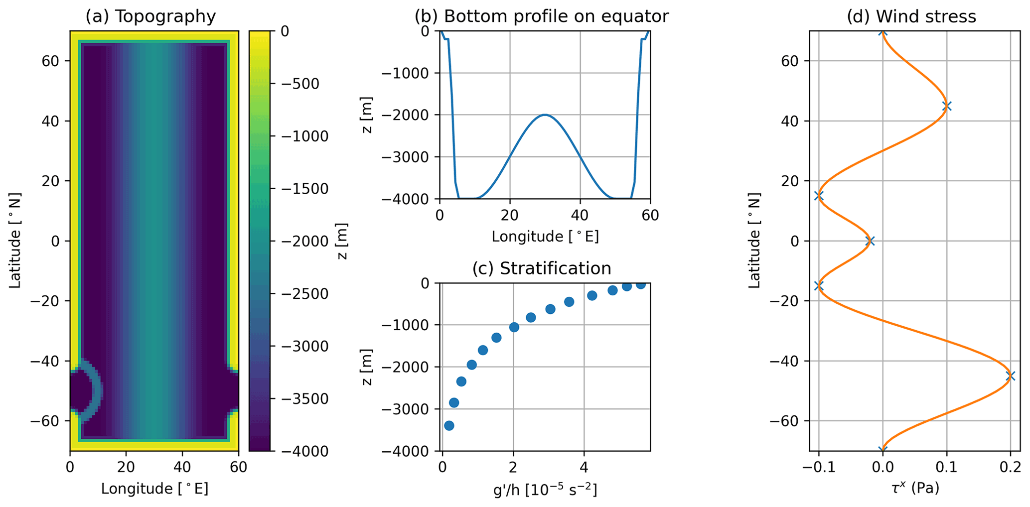
Figure 1NeverWorld2: (a) bathymetry (depth in meters); (b) cross-section of bathymetry on the Equator; (c) stratification, , at initial depths of each interface; (d) latitudinal profile of zonal wind stress forcing (in pascals), constructed from piecewise cubics with nodes indicated by crosses.
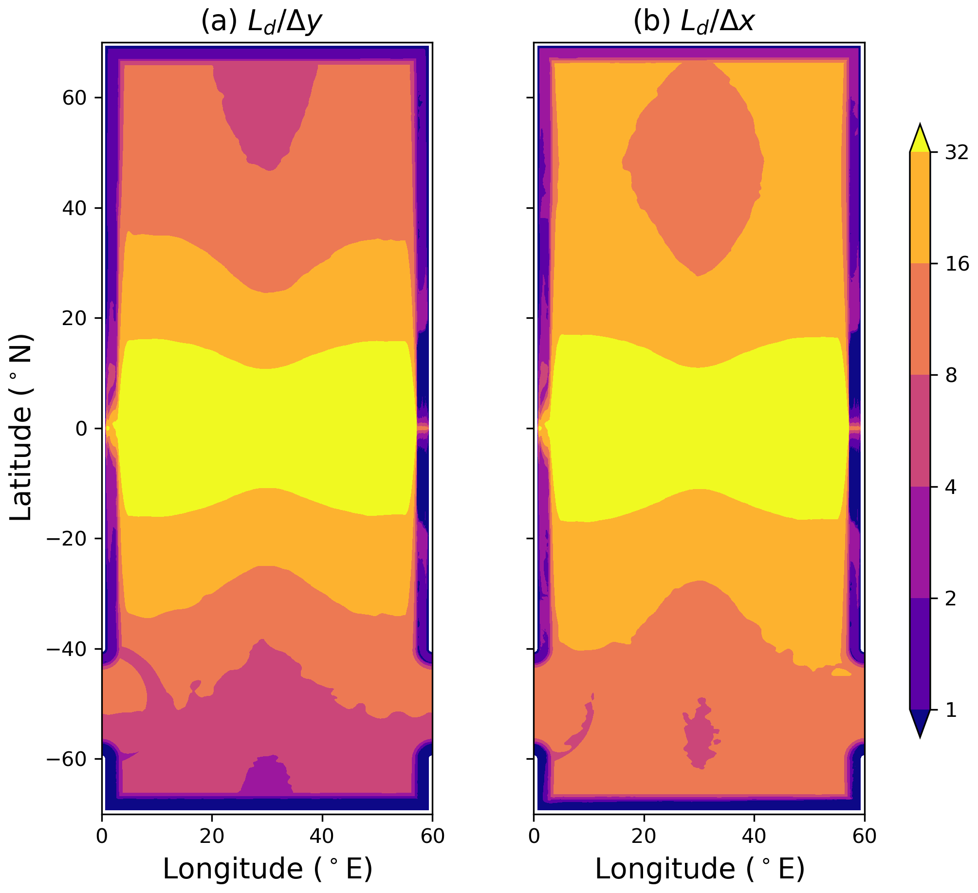
Figure 2(a) Meridional and (b) zonal resolution parameters, for the configuration, shown as the deformation radius Ld divided by the model meridional Δy or zonal Δx extent, respectively. The deformation scale is computed from the spun-up state. The aspect ratio between meridional and zonal extent is close to unity for most of the domain except for the very highest latitudes of the Southern Ocean, where the deformation radius is least well resolved.
2.1 Model equations
We consider an adiabatic and hydrostatic fluid system with a single thermodynamic constituent, simplified to a linear equation of state. This system can be approximated by N stacked layers of piecewise constant density. The equations of motion for the primary prognostic model variables, which are the zonal flow (u), meridional flow (v), and layer thickness (h), are written in vector-invariant form:
with the vertical stress divergence and horizontal friction given by
where a subscript k indicates the vertical layer number with k=1 the topmost and k=N the bottommost. We use the short-hand ∂t, ∂x, and ∂y for partial derivatives in time and in zonal and meridional directions, respectively. ∇⋅ is the horizontal divergence, ∇ the horizontal gradient, and the horizontal Laplacian. The MOM6 code (Adcroft et al., 2019) that discretizes these equations makes use of horizontal orthogonal curvilinear coordinates, though here we write the more concise Cartesian coordinate notation for brevity.
Other dynamic quantities that are derived from the primary variables include
-
the interface positions, , indicated with half-integer labels;
-
the potential vorticity, ;
-
the kinetic energy per mass, ;
-
the Montgomery potential, ;
-
the dynamic lateral viscosity, where Δ4 is the fourth power of the grid-spacing which follows a particular discretization, as proposed in the Appendix of Griffies and Hallberg (2000) and is different than simply using the square of the cell area;
-
the vertical stress, ;
-
the bottom stress, , which uses a quadratic drag law and where uB is the flow averaged over the bottommost 10 m.
The surface wind stress, , is prescribed, fixed in time, and distributed over the top 5 m. The remaining parameters are the reduced gravity of each layer, ; a reference density, ρo=1000 kg m−3; the Coriolis parameter, f=2Ωsin ϕ (with s−1, and ϕ is latitude); the background kinematic vertical viscosity, m2 s−1; a dimensionless bottom drag coefficient, Cd=0.003; and the bottom depth, . We have chosen to use a biharmonic dissipation operator with a dimensionless Smagorinsky coefficient of C4=0.2, which is larger than the recommended range suggested by Griffies and Hallberg (2000). This is to ensure sufficient dissipation in the absence of any other parameterizations of lateral friction. Other scale-aware alternatives (Bachman et al., 2017) arrived at comparable results.
We provide analysis of the energetics here and in subsequent papers (Loose et al., 2022b; Yankovsky et al., 2022). To facilitate such analysis, it is useful to write out the energy budget equations. The kinetic energy (KE) in layer k is given by KEk=hhKk. To obtain the KE equation, we add ukhk× Eq. (1), vkhk× Eq. (2), and Kk× Eq. (3), which gives
The contribution from the Coriolis terms, , should be zero in Eq. (6). However, the numerical model uses a C-grid staggering of variables so that locally the numerical Coriolis terms do not drop out, thus affecting KE. We use the Arakawa and Hsu (1990) discretization of Coriolis terms, which, when integrated over the whole domain, conserves total KE for horizontally non-divergent flow. The term ukhk⋅∇Mk is the conversion between potential energy and KE.
The potential energy (PE) at interface is given by . The corresponding PE equation is obtained by vertically summing equation (Eq. 3) from the bottom up to interface and then multiplying by :
When summed in the vertical, the right-hand side of Eq. (7) and the PE conversion term in Eq. (6) are equal.
The available potential energy (APE) is the domain-integrated PE minus the domain-integrated PE of the resting state. The resting state and interface positions used at initialization are given by , where is a constant nominal position for each interface. In this adiabatic model, changes in the domain-integrated PE are exactly the changes in APE, with no approximations or ambiguity.
2.2 Configuration
The NW2 configuration is set up as follows. The domain is a sector of a sphere with angular width 60∘ and with a single basin and a re-entrant channel in the Southern Hemisphere. The basin is bounded by solid coasts at 70∘ N and 70∘ S. Not extending to the poles avoids infinitesimal spherical coordinate cells as the meridians converge. We use a regular spherical grid rather than a Mercator grid so that the placement of boundaries (extents of the grid) is exactly the same for all resolutions. The regular spherical grid means the cells are distorted with cell-wise average aspect ratio , exceeding 2 only poleward of 60∘ N and 60∘ S. The full bathymetry is shown in Fig. 1a, with a cross-section along the Equator in Fig. 1b. The depth of the continental shelf is 200 m, and it has a nominal width of 2.5∘. A cubic profile, of width of the shelf, connects the shelf to the beach (which has zero depth out to of the shelf width). Another cubic profile of width 2.5∘ connects the shelf to the abyss with nominal depth of 4000 m. A large abyssal ridge of height 2000 m runs north–south down the middle of the basin with a cubic profile and radius of 20∘. The re-entrant channel spans 60–40∘ S, and a semi-circular ridge of height 2000 m, radius of 10∘, and thickness of 2∘ is centered on the channel opening in the west to block the deep flow through the channel. These deep ridges are idealizations of the Mid-Atlantic Ridge and the Scotia Arc that acts as a sill across the Drake Passage to remove momentum via form drag.
The wind stress is strictly zonal and fixed in time (Fig. 1b) and is an idealization of the mean zonal wind profile (see for example Fig. A1 of Chaudhuri et al., 2013). We construct the wind stress from piecewise cubic functions that interpolate between the values 0, 0.2, −0.1, −0.02, −0.1, 0.1, and 0 Pa at latitudes −70, −45, −15, 0, 15, 45, and 70∘, respectively. Each interpolation node has zero derivative so that both the wind stress and the curl of wind stress are zero at the north and south boundaries.
The initial stratification and vertical resolution are intimately linked (Fig. 1c). We use 15 layers and choose nominal thicknesses of 25, 50, 100, 125, 150, 175, 200, 225, 250, 300, 350, 400, 500, 550, and 600 m. The adiabatic conditions relieve the model of resolving surface boundary layer processes, but finer resolution near the surface is preserved to accurately capture surface intensification of mesoscale energy (Smith and Vallis, 2002). Actual initial thicknesses are the shallower of this nominal profile and whatever is clipped by topography to yield flat interfaces in the interior. The reduced gravity at each interface has values of 10, 0.0021, 0.0039, 0.0054, 0.0058, 0.0058, 0.0057, 0.0053, 0.0048, 0.0042, 0.0037, 0.0031, 0.0024, 0.0017, and 0.0011 m s−2. The first value corresponds to the gravitational acceleration at the surface. The implied density profile is approximately exponential with a depth scale of 1000 m (approximate due to rounding input parameter values to two significant digits).
The ratio between the first baroclinic deformation radius (LD) to the meridional and zonal grid spacing is shown in Fig. 2a and b, respectively. Assuming that to resolve eddies, (Hallberg, 2013), Fig. 2 highlights that the horizontal resolution simulation explicitly resolves mesoscale eddies, except on the shelves and at very high latitudes of the Southern Ocean.
The model is initialized from rest at horizontal grid spacing, with initial conditions described in Sect. 2.2 and depicted in Fig. 1c. The simulation is run to a quasi-steady state reached by about 3×10⁴ d, in which the total kinetic energy is no longer drifting. Next, the layer thicknesses are interpolated to the horizontal grid, and the simulation is run again to a quasi-steady state for a few thousand days. Note that for expediency, velocities and transports are not interpolated but rather reset to zero. This step introduces a mild shock, but the model quickly spins up mechanically, as seen in the recovery of kinetic energy levels in Fig. 3. This procedure is repeated for and horizontal grids until the simulation has reached convergence (see Sect. 5 for further description).
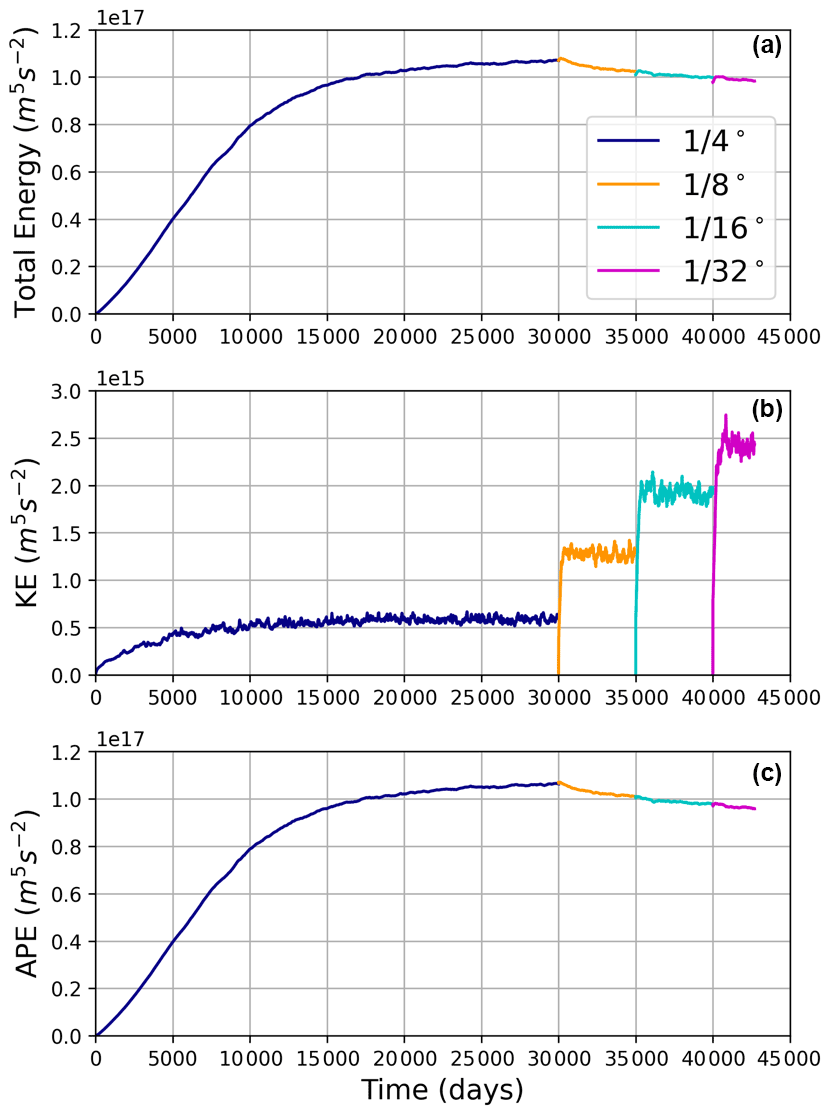
Figure 3Time series of total energy (a), kinetic energy (b), and available potential energy (c) as a function of time for all horizontal grids considered during spinup and equilibration.
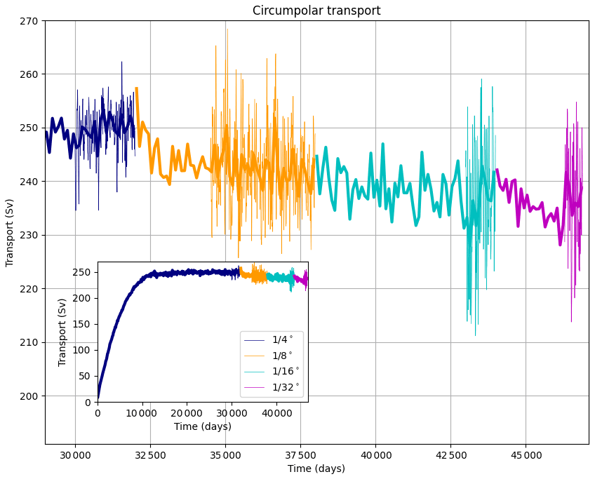
Figure 4Time series of ACC transport, defined as the total (zonal) transport across longitude 0∘ E for each of the model horizontal grids during spinup and equilibration. Thin lines are 5 d means (where available), and thicker lines are 100 d means. The inset shows the entire time series, which starts from the configuration at rest.
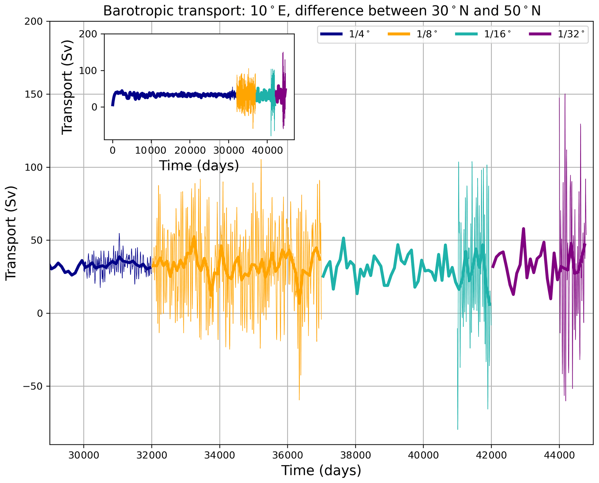
Figure 5Time series of the difference in the barotropic transport stream function at 10 ∘ E between 30 and 50∘ N for each of the model horizontal grids during spinup and equilibrium. Thin lines are 5 d means (where available), and thicker lines are 100 d means. The inset shows the entire time series, which starts from the configuration at rest.

Figure 6Time series of equatorial thermocline depth, defined here as the depth of the fourth layer, at longitude 15∘ E for each of the model horizontal grids during spinup and equilibration. Thin lines are 5 d means (where available), and thicker lines are 100 d means.
As the model horizontal grid is refined, the total kinetic energy (KE) increases at each transition to finer spacing (Fig. 3); this behavior is expected since the finer dynamical modes contain more kinetic energy. In addition, the available potential energy (APE) decreases at each transition to finer grids possibly because eddies are numerically better resolved and become more efficient at extracting APE. The total energy of the system drops at each transition in grid spacing, since APE dominates the total energy reservoir, but the drop is less than for APE due to the increase in KE.
The circumpolar transport spins up in ∼104 d (Fig. 4) and fluctuates with no discernible drift for the remaining 2×10⁴ d at . There is a small reduction in circumpolar transport at each refinement in grid spacing, just as for APE. Since the baroclinic component of circumpolar transport is related to APE, arguments about the improved efficiency of eddies with refined grid spacing are relevant (Marshall and Radko, 2003).
The difference in barotropic transport stream function between sub-tropical and subpolar regions spins up in ∼ 3000–4000 d in the simulation and fluctuates without discernible drift for the remaining 2.5×10⁴ d (Fig. 5). This adjustment time is consistent with basin travel times for mid-latitude baroclinic Rossby waves (∼2 cm s−1). The transition to finer grid spacing does lead to an increase in the variability. However, the time mean of this transport index does not change significantly with grid spacing, as expected via Sverdrup theory.
The equatorial thermocline depth at 15∘ E adjusts on multiple timescales with large oscillations at the start of the simulation that damp out over ∼ 4000 d (Fig. 6). A statistical equilibrium depth is reached on the order of ∼104 d. There is an adjustment at each transition in grid spacing, but it is smaller than the dynamical noise.
During the spinup, the model exhibits multiple timescales in the diagnostics described. The cost of the spinup to day 4.2×10⁴ (covering , , and ) is ∼ 17 % of the cost of the 2800 d segment at resolution. The initialization procedure of consecutively allowing adjustment and then interpolating to finer grids is approximately 75× cheaper than spinning up the model solution entirely at .
We illustrate the behavior of the model in terms of key properties of the flow, with a focus on transport and energy reservoirs. We compare the high-resolution NW2 with a horizontal grid, in which mesoscale eddies are explicitly resolved in the majority of the domain, to lower-resolution NW2 with horizontal grids of , , and . No mesoscale eddy closures are used in any of the simulations beyond the Smagorinsky friction.

Figure 7Time-mean barotropic transport stream function (Sv) averaged over the last 500 d of each simulation. Transport contours are shown every 10 Sv.
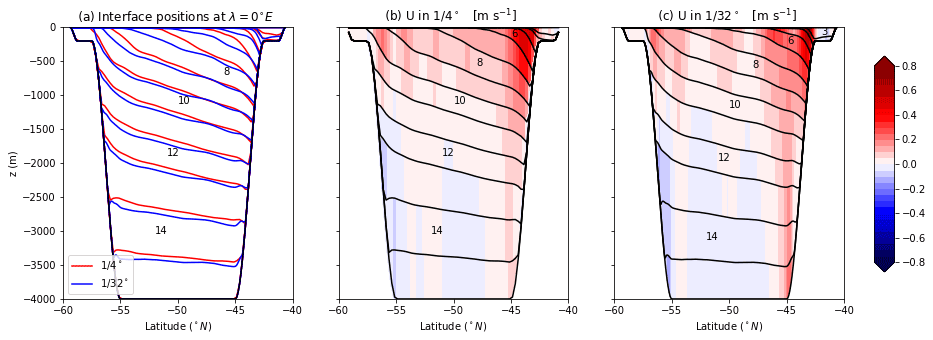
Figure 8(a) Mean hydrography across the southern channel (Drake Passage) for and models, depicted by time-mean position of interfaces (isopycnals). Time-mean zonal flow (contour interval of 0.05 m s−1), with interface positions for models at (b) and (c) horizontal grids, respectively. All results are averages over 500 d at longitude 0∘ E, with eastward flow red and westward flow blue.

Most of the large-scale features of the finest-resolution configuration are recognizable in the coarsest-resolution solution. The time-mean circulation is represented by subtropical gyres in both hemispheres, a subpolar gyre in the Northern Hemisphere (Fig. 7), and a series of circumpolar jets in the Southern Hemisphere reminiscent of the Antarctic Circumpolar Current (ACC) (Figs. 8 and 9). As the grid spacing is refined, the strength of the western boundary currents and their extensions seems to increase (Fig. 7), while the circumpolar jet (Fig. 4) decreases slightly (proportionally).
The thermocline depth along the Equator also barely changes with resolution (Fig. 6). Overall, the character of the large-scale circulation is relatively invariant with resolution even though the metrics of various features converge with finer resolution.
Some details of the circulation that differ across resolution include, for example, major differences in upper-ocean stratification in the Southern Ocean between the coarsest and finest resolutions. The interfaces in the fine-resolution simulation are less steep, and the interface outcrops move southward as a result of re-stratification by eddies (Fig. 8a). As the grid spacing is refined, the vertical extent of jets changes (Fig. 8). The time-mean zonal velocity shows either a change in the number of distinct jets or a migration of mean jet position. Most notable is the appearance of a deep westward circulation in the channel, below the depth of the blocking topography (the Scotia Arc downstream of the passage).
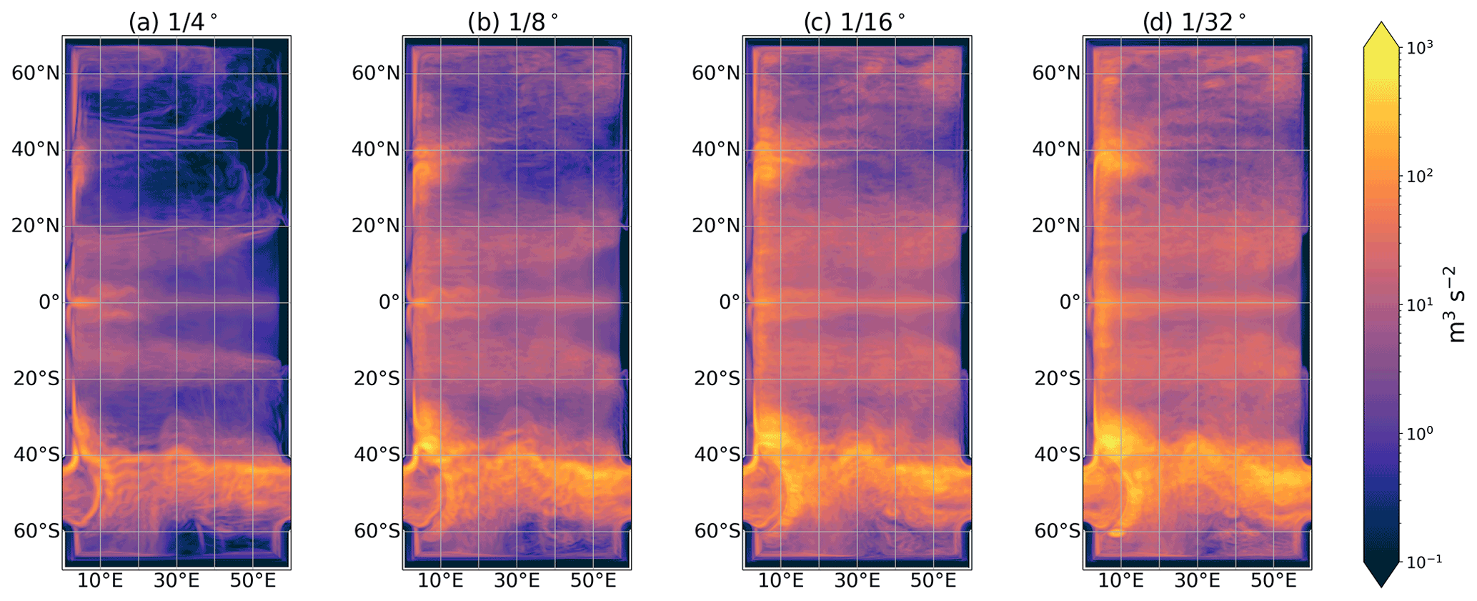
Snapshots of depth-integrated KE reveal the eddying behavior of the simulations (Fig. 9). For the coarsest grid (), the flow permits mesoscale eddies, in particular at low latitudes, where the deformation scale is largest. As the grid spacing is refined, the first deformation radius is better resolved, and mesoscale eddies become more ubiquitous and widespread. Note that a casual glance does not readily distinguish the and models.
The time mean of depth-integrated total KE (Fig. 10) becomes spatially smoother at finer grid spacing as eddies become increasingly ubiquitous. The same is true for sea surface height variance (not shown), a frequently used indicator of eddy activity.
Defining convergence for a turbulent cascade is challenging when using a dynamic viscosity because finer grid spacing will permit ever more variability on finer scales. For the purposes of mesoscale eddies, we are concerned with convergence as manifested by invariance of the large-scale properties as resolution changes, thus implying the upscale transfer of kinetic energy is not changing so that details of the small scales are not affecting the large-scale solution.
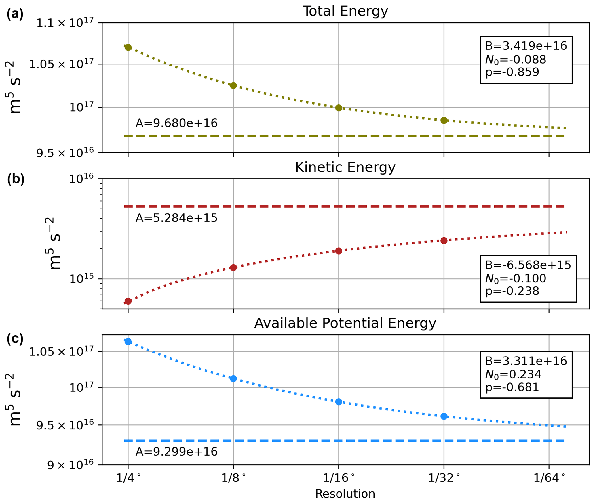
Figure 11Equilibrium total energy, kinetic energy (KE), and available potential energy (APE) as a function of horizontal resolution (), averaged over the last 500 d of each simulation. Note the different scale used for KE (b). The dotted lines are a fit of the form , and the asymptotic limit, A, is indicated by the dashed line.
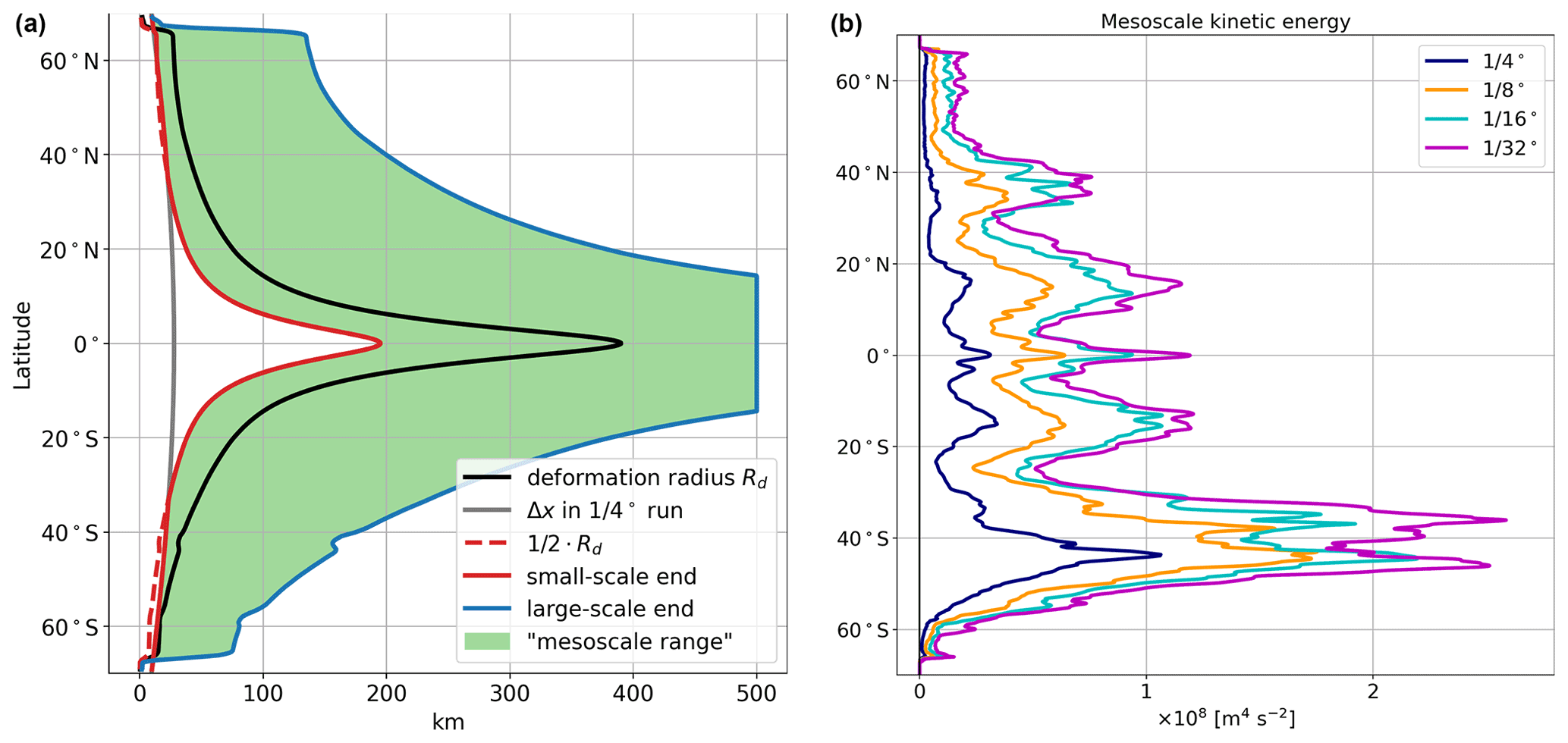
Figure 12(a) Definition of our band-pass filter to extract the mesoscale range (green shading). The small-scale end (solid red line) of the mesoscale range is defined as max(0.5 Rd,Δx), where Δx is the longitudinal grid spacing in the 1/4∘ degree run. The large-scale end (blue line) of the mesoscale range is defined as min(5 Rd, 500 km), where Rd is the first baroclinic deformation radius diagnosed from the NeverWorld2 simulations; (b) 500 d averaged, zonally and depth-integrated mesoscale kinetic energy for the four simulations in our model hierarchy. The mesoscale kinetic energy is computed via the band-pass filter defined on the left.
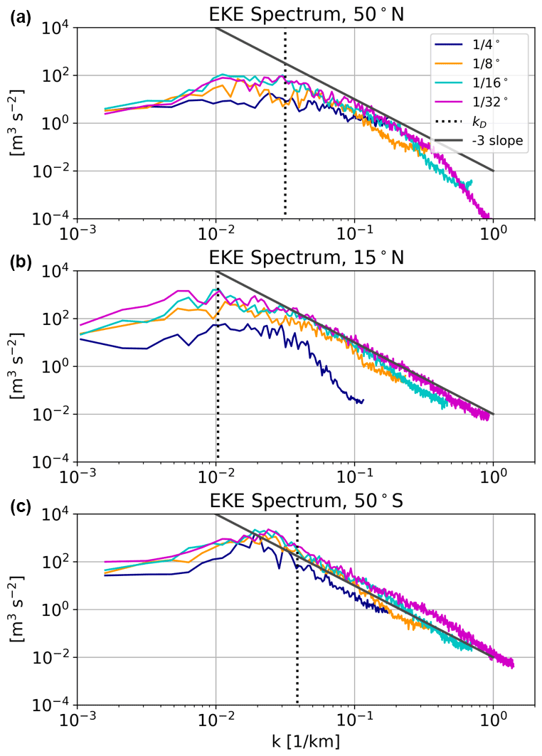
Figure 13The 100 d averaged zonal (one-dimensional) spectra of surface EKE for all resolutions at three latitudes (top to bottom): 50∘ N (weak mean flow region), 15∘ N (mid-latitude gyre), and 50∘ S (ACC). We employ the XRFT Python package (Uchida et al., 2021) for the calculations of spectra. Spectra are computed from the surface meridional eddy velocity fields, defined as deviations from a 100 d averaged meridional velocity. Meridional velocities are less influenced by temporal fluctuations in the large-scale zonal currents and allow a better visualization of mesoscale eddy influences. The 2.5∘ of data are cut off from the eastern and western boundaries before computing the spectra, and linear detrending and a Hann smoothing window are applied. The wavenumber kD corresponding to the deformation radius for the simulation is shown as a dotted black line, and a −3 spectral slope is shown in gray. Note that the high-wavenumber spectral tails are sensitive to smoothing choice and boundary effects.
The total mechanical energy of the system (APE + KE reservoirs) is dominated by the APE. APE is an integral metric of the system and the reservoir of energy that generates mesoscale eddies. In equilibrium, there is a balance of APE generation by winds (pumping/heaving the isopycnals) and the conversion of APE to mesoscale eddy energy and the subsequent damping of mean and mesoscale energy by bottom drag, Smagorinsky friction, and vertical viscosity. The equilibrium levels of energy reservoirs shown in Fig. 11 indicate a diminishing APE transition for each change in grid spacing, with an empirical fit suggesting convergence towards a value that is about 3 % lower than the value in the simulation. We suggest that this behavior implies we are approaching convergence for resolving the mean APE-to-eddy energy pathway.
The kinetic energy increases less than linearly as grid spacing is refined (middle panel of Figs. 3 and 11); there is a 5-fold increase in the kinetic energy reservoir between the and the simulations. A power law fit indicates convergence but not until kinetic energy is about another factor of 2 higher than in the simulation.
To test convergence of the mesoscale, Fig. 12b shows the 500 d averaged, zonally and depth-integrated mesoscale kinetic energy. The mesoscale kinetic energy is computed with a band-pass filter as .
Here, and denote low-pass filters, with filter scales defined by the red and blue solid lines in Fig. 12a, respectively.
For the respective filter operations, we use the Python package gcm-filters (Loose et al., 2022a) with a Gaussian filter shape.
As the horizontal grid spacing is refined from to , we observe steadily growing mesoscale eddy activity in all regions of the domain (Fig. 12b), but the increase from to is smaller compared to the increase from to and from to . An exception is the energetic recirculation region north of Drake Passage near 38∘S, where the mesoscale kinetic energy increases considerably as we change the grid spacing from to . We speculate that this increase is due to large-scale standing meanders that develop north of Drake Passage due to more finely resolved topography (Kong and Jansen, 2020; Barthel et al., 2017).
The zonal wavenumber spectra of EKE at various latitudes (Fig. 13) show that at all latitudes, there is a clear gain in kinetic energy between the and the simulations, at all wavenumbers. At higher resolutions, a pronounced peak in the EKE at scales at or slightly above the deformation scale develops. The peak is the result of an increasingly resolved mesoscale eddy-driven inverse KE cascade. The notable exception is the ACC region, where there is less sensitivity to resolution. As hinted by the snapshots of KE, convergence at low latitude is achieved faster than at high latitudes. The spectra generally suggest the large scales are more similar between and , although full convergence has not yet been obtained.
In this paper, we introduce an idealized ocean model configuration, NeverWorld2 (NW2), that resolves mesoscale eddy dynamics in a basin-scale context. NW2 is a stacked shallow-water model using the MOM6 dynamical core (Adcroft et al., 2019), configured with a single cross-equatorial basin and a re-entering channel in the Southern Hemisphere with idealized geometry. Because NW2 is strictly adiabatic, with no parameterizations in the vertical direction, the timescales of adjustment are controlled entirely by dynamics rather than far slower thermodynamic processes. The paper serves as an introduction to the model and grid resolution hierarchy and to the datasets for use by the community.
For the purposes of analyzing the role of mesoscale eddies and deriving and testing parameterizations, we provide evidence that the finest grid spacing shown, , is practically converged. The large-scale metrics of APE and gyre transport, the latitudinal analysis of KE, and the spectral analysis of EKE all suggest convergence of the largest scales when comparing solutions with the and grid spacings.
We have used the Smagorinsky dynamic biharmonic viscosity of Griffies and Hallberg (2000) for the momentum closure in these simulations, including for the finest grid spacing that defines our converged “truth”. Previous work has shown a sensitivity of the details of the forward and inverse turbulent cascade to the form of dissipation (e.g., Smith and Vallis, 2002; Arbic and Flierl, 2004; Thompson and Young, 2007; Arbic et al., 2012; Pietarila Graham and Ringler, 2013; Soufflet et al., 2016; Pearson et al., 2017; Bachman et al., 2017; Treguier et al., 1997). In refining grid spacing here, we seek to converge on resolving the mechanism of interaction between the mesoscale eddies and the large-scale circulation, by showing it to be diminishingly dependent on the details of dissipation near the bottom of the forward enstrophy cascade; this dissipation scale is more and more separated from the eddy production scale. This assumption could be tested by trying alternative closures and evaluating what tuning is necessary to give the same upscale energy flux. We could have used one of several closures proposed as scale-aware schemes to use in the eddy-permitting regime (e.g., Anstey and Zanna, 2017; Bachman et al., 2017). However, using them in the baseline configuration described here would hinder a fair evaluation of those schemes, which we plan to do in the near future. Nevertheless, we acknowledge that the absolute magnitude of eddy energy, the span of the inverse cascade, and other metrics depend somewhat on the choice of viscous closure.
The model spatial-resolution hierarchy, from coarse to eddy-rich, allows for a clean and extensive analysis of the dynamics and energetics of the flow as a function of horizontal grid spacing, which will be upcoming. The coarser grid configurations shown here can serve as a test bed for the evaluation of scale-aware mesoscale eddy parameterizations in the “gray” zone of eddy-permitting resolution. Even coarser, non-eddying configurations, not shown here because they need an eddy parameterization to look sensible, will be used to evaluate parameterizations of subgrid mesoscale eddies.
One virtue of the NW2 model is that the adiabatic limit isolates mesoscale eddies from other processes. However, there are strong interactions between mesoscale eddies and the surface mixed layer which have been recognized since early evaluations of mesoscale parameterizations (Danabasoglu et al., 1994). The dynamical core and algorithm used are the same as for a the full primitive-equation general circulation model (Adcroft et al., 2019; Griffies et al., 2020), so adding diabatic processes is relatively straightforward. The NW2 model can be modified and developed further to explore the large-scale overturning circulation (e.g., Wolfe and Cessi, 2009) or the connection with other parameterizations, for example, mixed-layer and sub-mesoscale parameterizations.
The MOM6 source code, NW2 configuration files, and plotting and analysis scripts used in this article are available at https://doi.org/10.5281/zenodo.6993951 (Bhamidipati et al., 2022). The NW2 dataset and detailed information on its contents are available at https://doi.org/10.26024/f130-ev71 (Marques et al., 2022).
GMM, NL, NB, JS, EY, CYC, AA, MFJ, RWH, and LZ contributed to the development and analysis of NW2 configurations. GMM, NL, JS, EY, AA, and LZ led the manuscript, and SMG, BFK, MFJ, and HK contributed to the manuscript.
The contact author has declared that none of the authors has any competing interests.
The statements, findings, conclusions, and recommendations are those of the author(s) and do not necessarily reflect the views of the National Oceanic and Atmospheric Administration or the US Department of Commerce.
Publisher's note: Copernicus Publications remains neutral with regard to jurisdictional claims in published maps and institutional affiliations.
We thank all the members of the Ocean Transport and Eddy Energy Climate Process Team for helpful discussions during the design, implementation, and evaluation of the NW2 simulations. We also thank the editor, Qiang Wang, as well as Takaya Uchida and an anonymous reviewer for their constructive comments that helped to improve the quality and presentation of this paper. Gustavo M. Marques was supported by National Science Foundation (NSF) grant OCE 1912420. Chiung-Yin Chang and Neeraja Bhamidipati were supported by award NA19OAR4310365 and Alistair Adcroft by award NA18OAR4320123, from the National Oceanic and Atmospheric Administration (NOAA), US Department of Commerce. Laure Zanna and Elizabeth Yankovsky were supported by NSF grant OCE 1912357 and NOAA CVP NA19OAR4310364. Baylor Fox-Kemper is supported by NOAA NA19OAR4310366. Laure Zanna is supported by NSF grant OCE 1912332. Malte F. Jansen is supported by NSF grant OCE 1912163. Jacob M. Steinberg is supported by NSF grant OCE 1912302. Hemant Khatri acknowledges the support from Natural Environment Research Council (NERC) grant NE/T013494/1 and NOAA grant NA18OAR4320123. Stephen M. Griffies and Robert W. Hallberg acknowledge support from the National Oceanic and Atmospheric Administration Geophysical Fluid Dynamics Laboratory. This material is also based upon work supported by the National Center for Atmospheric Research (NCAR), which is a major facility sponsored by the NSF under cooperative agreement no. 1852977. Computing and data storage resources, including the Cheyenne supercomputer, were provided by the Computational and Information Systems Laboratory at NCAR, under NCAR/CISL project number UNYU0004.
This research has been supported by the US Department of Commerce (grant no. NA18OAR4320123), the Division of Ocean Sciences (grant nos. 1912420, 1912332, 1912357, 1912163, and 1912302), the Division of Atmospheric and Geospace Sciences (grant no. 1852977), and the Climate Program Office (grant nos. NA19OAR4310364, NA19OAR4310365, and NA19OAR4310366).
This paper was edited by Qiang Wang and reviewed by Takaya Uchida and one anonymous referee.
Adcroft, A., Anderson, W., Balaji, V., Blanton, C., Bushuk, M., Dufour, C. O., Dunne, J. P., Griffies, S. M., Hallberg, R. W., Harrison, M. J., Held, I., Jansen, M. F., John, J., Krasting, J. P., Langenhorst, A., Legg, S., Liang, Z., McHugh, C., Radhakrishnan, A., Reichl, B. G., Rosati, T., Samuels, B. L., Shao, A., Stouffer, R., Winton, M., Wittenberg, A. T., Xiang, B., Zadeh, N., and Zhang, R.: The GFDL Global Ocean and Sea Ice Model OM4.0: Model Description and Simulation Features, J. Adv. Model. Earth Sy., 11, 3167–3211, https://doi.org/10.1029/2019MS001726, 2019. a, b, c, d
Anstey, J. A. and Zanna, L.: A deformation-based parametrization of ocean mesoscale eddy reynolds stresses, Ocean Model., 112, 99–111, https://doi.org/10.1016/j.ocemod.2017.02.004, 2017. a
Arakawa, A. and Hsu, Y.-J. G.: Energy Conserving and Potential-Enstrophy Dissipating Schemes for the Shallow Water Equations, Mon. Weather Rev., 118, 1960–1969, https://doi.org/10.1175/1520-0493(1990)118<1960:ECAPED>2.0.CO;2, 1990. a
Arbic, B. K. and Flierl, G. R.: Baroclinically Unstable Geostrophic Turbulence in the Limits of Strong and Weak Bottom Ekman Friction: Application to Midocean Eddies, J. Phys. Oceanogr., 34, 2257–2273, https://doi.org/10.1175/1520-0485(2004)034<2257:BUGTIT>2.0.CO;2, 2004. a, b
Arbic, B. K., Scott, R. B., Flierl, G. R., Morten, A. J., Richman, J. G., and Shriver, J. F.: Nonlinear Cascades of Surface Oceanic Geostrophic Kinetic Energy in the Frequency Domain, J. Phys. Oceanogr., 42, 1577–1600, https://doi.org/10.1175/JPO-D-11-0151.1, 2012. a
Bachman, S. D.: The GM+E closure: A framework for coupling backscatter with the Gent and McWilliams parameterization, Ocean Model.g, 136, 85–106, https://doi.org/10.1016/j.ocemod.2019.02.006, 2019. a
Bachman, S. D., Fox-Kemper, B., and Pearson, B.: A scale-aware subgrid model for quasi-geostrophic turbulence, J. Geophys. Res.-Oceans, 122, 1529–1554, https://doi.org/10.1002/2016JC012265, 2017. a, b, c
Barthel, A., Hogg, A. M., Waterman, S., and Keating, S.: Jet–Topography Interactions Affect Energy Pathways to the Deep Southern Ocean, J. Phys. Oceanogr., 47, 1799–1816, https://doi.org/10.1175/JPO-D-16-0220.1, 2017. a
Bhamidipati, N., Adcroft, A., Marques, G., and Abernathey, R.: ocean-eddy-cpt/NeverWorld2: NeverWorld2-description-paper (v1.1), Zenodo [code], https://doi.org/10.5281/zenodo.6993951, 2022. a
Cessi, P.: An Energy-Constrained Parameterization of Eddy Buoyancy Flux, J. Phys. Oceanogr., 38, 1807–1819, https://doi.org/10.1175/2007JPO3812.1, 2008. a
Chaudhuri, A. H., Ponte, R. M., Forget, G., and Heimbach, P.: A Comparison of Atmospheric Reanalysis Surface Products over the Ocean and Implications for Uncertainties in Air–Sea Boundary Forcing, J. Climate, 26, 153–170, https://doi.org/10.1175/JCLI-D-12-00090.1, 2013. a
Chelton, D. B., deSzoeke, R. A., Schlax, M. G., El Naggar, K., and Siwertz, N.: Geographical Variability of the First Baroclinic Rossby Radius of Deformation, J. Phys. Oceanogr., 28, 433–460, https://doi.org/10.1175/1520-0485(1998)028<0433:GVOTFB>2.0.CO;2, 1998. a
Danabasoglu, G., McWilliams, J. C., and Gent, P. R.: The Role of Mesoscale Tracer Transports in the Global Ocean Circulation, Science, 264, 1123–1126, https://doi.org/10.1126/science.264.5162.1123, 1994. a
Eden, C. and Greatbatch, R. J.: Towards a mesoscale eddy closure, Ocean Model., 20, 223–239, https://doi.org/10.1016/j.ocemod.2007.09.002, 2008. a
Gent, P. R. and McWilliams, J. C.: Isopycnal Mixing in Ocean Circulation Models, J. Phys. Oceanogr., 20, 150–155, https://doi.org/10.1175/1520-0485(1990)020<0150:IMIOCM>2.0.CO;2, 1990. a
Gent, P. R., Willebrand, J., McDougall, T. J., and McWilliams, J. C.: Parameterizing Eddy-Induced Tracer Transports in Ocean Circulation Models, J. Phys. Oceanogr., 25, 463–474, https://doi.org/10.1175/1520-0485(1995)025<0463:PEITTI>2.0.CO;2, 1995. a
Griffies, S. M. and Hallberg, R. W.: Biharmonic Friction with a Smagorinsky-Like Viscosity for Use in Large-Scale Eddy-Permitting Ocean Models, Mon. Weather Rev., 128, 2935–2946, https://doi.org/10.1175/1520-0493(2000)128<2935:BFWASL>2.0.CO;2, 2000. a, b, c
Griffies, S. M., Adcroft, A., and Hallberg, R. W.: A Primer on the Vertical Lagrangian-Remap Method in Ocean Models Based on Finite Volume Generalized Vertical Coordinates, J. Adv. Model. Earth Sy., 12, e2019MS001954, https://doi.org/10.1029/2019MS001954, 2020. a
Hallberg, R.: Using a resolution function to regulate parameterizations of oceanic mesoscale eddy effects, Ocean Model., 72, 92–103, https://doi.org/10.1016/j.ocemod.2013.08.007, 2013. a, b, c
Hewitt, H. T., Roberts, M., Mathiot, P., Biastoch, A., Blockley, E., Chassignet, E. P., Fox-Kemper, B., Hyder, P., Marshall, D. P., Popova, E., Treguier, A.-M., Zanna, L., Yool, A., Yu, Y., Beadling, R., Bell, M., Kuhlbrodt, T., Arsouze, T., Bellucci, A., Castruccio, F., Gan, B., Putrasahan, D., Roberts, C. D., Van Roekel, L., and Zhang, Q.: Resolving and Parameterising the Ocean Mesoscale in Earth System Models, Current Climate Change Reports, 6, 137–152, https://doi.org/10.1007/s40641-020-00164-w, 2020. a
Jansen, M. F. and Held, I. M.: Parameterizing subgrid-scale eddy effects using energetically consistent backscatter, Ocean Model., 80, 36–48, https://doi.org/10.1016/j.ocemod.2014.06.002, 2014. a
Jansen, M. F., Adcroft, A., Khani, S., and Kong, H.: Toward an Energetically Consistent, Resolution Aware Parameterization of Ocean Mesoscale Eddies, J. Adv. Model. Earth Sy., 11, 2844–2860, https://doi.org/10.1029/2019MS001750, 2019. a, b
Khani, S., Jansen, M. F., and Adcroft, A.: Diagnosing subgrid mesoscale eddy fluxes with and without topography, J. Adv. Model. Earth Sy., 11, 3995–4015, https://doi.org/10.1029/2019MS001721, 2019. a
Kjellsson, J. and Zanna, L.: The Impact of Horizontal Resolution on Energy Transfers in Global Ocean Models, Fluids, 2, 45, https://doi.org/10.3390/fluids2030045, 2017. a
Kong, H. and Jansen, M. F.: The impact of topography and eddy parameterization on the simulated Southern Ocean circulation response to changes in surface wind stress, J. Phys. Oceanogr., 1, 825–843, https://doi.org/10.1175/JPO-D-20-0142.1, 2020. a
Loose, N., Abernathey, R., Grooms, I., Busecke, J., Guillaumin, A., Yankovsky, E., Marques, G., Steinberg, J., Ross, A. S., Khatri, H., Bachman, S., Zanna, L., and Martin, P.: GCM-Filters: A Python Package for Diffusion-based Spatial Filtering of Gridded Data, J. Open Source Softw., 7, 3947, https://doi.org/10.21105/joss.03947, 2022a. a
Loose, N., Bachman, S., GROOMS, I., and Jansen, M.: Diagnosing scale-dependent energy cycles in a high-resolution isopycnal ocean model, Earth and Space Science Open Archive [data set], https://doi.org/10.1002/essoar.10511055.1, 2022b. a
Marques, G., Loose, N., Yankovsky, E., Steinberg, J., Chang, C.-Y., Bhamidipati, N., Adcroft, A., Fox-Kemper, B., Griffies, S., Hallberg, R., Jansen, M., Khatri, H., and Zanna, L.: NeverWorld2 Dataset, NeverWorld2 [data set], https://doi.org/10.26024/f130-ev71, 2022. a
Marshall, D. P. and Adcroft, A. J.: Parameterization of ocean eddies: Potential vorticity mixing, energetics and Arnold's first stability theorem, Ocean Model., 32, 188–204, https://doi.org/10.1016/j.ocemod.2010.02.001, 2010. a
Marshall, D. P., Maddison, J. R., and Berloff, P. S.: A Framework for Parameterizing Eddy Potential Vorticity Fluxes, J. Phys. Oceanogr., 42, 539–557, https://doi.org/10.1175/JPO-D-11-048.1, 2012. a
Marshall, J. and Radko, T.: Residual-Mean Solutions for the Antarctic Circumpolar Current and Its Associated Overturning Circulation, J. Phys. Oceanogr., 33, 2341–2354, https://doi.org/10.1175/1520-0485(2003)033<2341:RSFTAC>2.0.CO;2, 2003. a
McClean, J. L., Bader, D. C., Bryan, F. O., Maltrud, M. E., Dennis, J. M., Mirin, A. A., Jones, P. W., Kim, Y. Y., Ivanova, D. P., Vertenstein, M., Boyle, J. S., Jacob, R. L., Norton, N., Craig, A., and Worley, P. H.: A prototype two-decade fully-coupled fine-resolution CCSM simulation, Ocean Model., 39, 10–30, https://doi.org/10.1016/j.ocemod.2011.02.011, 2011. a
Pearson, B., Fox-Kemper, B., Bachman, S., and Bryan, F.: Evaluation of scale-aware subgrid mesoscale eddy models in a global eddy-rich model, Ocean Model., 115, 42–58, https://doi.org/10.1016/j.ocemod.2017.05.007, 2017. a
Pietarila Graham, J. and Ringler, T.: A framework for the evaluation of turbulence closures used in mesoscale ocean large-eddy simulations, Ocean Model., 65, 25–39, https://doi.org/10.1016/j.ocemod.2013.01.004, 2013. a
Smith, K. S. and Vallis, G. K.: The Scales and Equilibration of Midocean Eddies: Forced–Dissipative Flow, J. Phys. Oceanogr., 32, 1699–1720, https://doi.org/10.1175/1520-0485(2002)032<1699:TSAEOM>2.0.CO;2, 2002. a, b, c
Soufflet, Y., Marchesiello, P., Lemarié, F., Jouanno, J., Capet, X., Debreu, L., and Benshila, R.: On effective resolution in ocean models, Ocean Model., 98, 36–50, https://doi.org/10.1016/j.ocemod.2015.12.004, 2016. a
Thompson, A. F. and Young, W. R.: Two-Layer Baroclinic Eddy Heat Fluxes: Zonal Flows and Energy Balance, J. Atmos. Sci., 64, 3214–3231, https://doi.org/10.1175/JAS4000.1, 2007. a, b
Treguier, A. M., Held, I. M., and Larichev, V. D.: Parameterization of Quasigeostrophic Eddies in Primitive Equation Ocean Models, J. Phys. Oceanogr., 27, 567–580, https://doi.org/10.1175/1520-0485(1997)027<0567:POQEIP>2.0.CO;2, 1997. a
Uchida, T., Rokem, A., Nicholas, T., Abernathey, R., Nouguier, F., Vanderplas, J., Martin, P., Mayer, A., Halchenko, Y., Wilson, G., Constantinou, N. C., Ponte, A., Squire, D., Busecke, J., Spring, A., Pak, K., and Hoyer, S.: xgcm/xrft: v0.3.1-rc0, https://doi.org/10.5281/zenodo.5503856, 2021. a
Wolfe, C. L. and Cessi, P.: Overturning Circulation in an Eddy-Resolving Model: The Effect of the Pole-to-Pole Temperature Gradient, J. Phys. Oceanogr., 39, 125–142, https://doi.org/10.1175/2008JPO3991.1, 2009. a, b
Yankovsky, E., Zanna, L., and Smith, K. S.: Influences of Mesoscale Ocean Eddies on Flow Vertical Structure in a Resolution-Based Model Hierarchy, Earth and Space Science Open Archive, https://doi.org/10.1002/essoar.10511501.1, 2022. a