wavetrisk-2.1: an adaptive dynamical core for ocean modelling

This paper introduces wavetrisk-2.1 (i.e. wavetrisk-ocean), an incompressible version of the atmosphere model wavetrisk-1.x with free surface. This new model is built on the same wavelet-based dynamically adaptive core as wavetrisk, which itself uses dynamico's mimetic vector-invariant multilayer rotating shallow water formulation. Both codes use a Lagrangian vertical coordinate with conservative remapping. The ocean variant solves the incompressible multilayer shallow water equations with inhomogeneous density layers. Time integration uses barotropic–baroclinic mode splitting via an semi-implicit free surface formulation, which is about 34–44 times faster than an unsplit explicit time-stepping. The barotropic and baroclinic estimates of the free surface are reconciled at each time step using layer dilation. No slip boundary conditions at coastlines are approximated using volume penalization. The vertical eddy viscosity and diffusivity coefficients are computed from a closure model based on turbulent kinetic energy (TKE). Results are presented for a standard set of ocean model test cases adapted to the sphere (seamount, upwelling and baroclinic turbulence). An innovative feature of wavetrisk-ocean is that it could be coupled easily to the wavetrisk atmosphere model, thus providing a first building block toward an integrated Earth system model using a consistent modelling framework with dynamic mesh adaptivity and mimetic properties.

1 Introduction

Dynamically adaptive methods have the potential to significantly improve the computational efficiency and accuracy of the dynamical cores of atmosphere and ocean models. They do this by optimizing grid resolution at each time step to represent the dynamically active parts of the flow. This makes better use of computational resources by using fine resolution where needed and also allows better control of accuracy since the grid may be adapted based on a local error indicator. The same technique can also be used to build statically adapted “nested” models which avoid reflection and other errors at the refinement boundaries. Another feature of adaptive methods is that they can be run at coarse resolutions for long times to spin up a model and then easily restarted with much higher resolutions for shorter runs.

However, these advantages come at the cost of increased code complexity and it is not clear a priori whether dynamically adaptive methods will work well in complex multi-physics simulations with separate subgrid-scale (SGS) parameterizations. Because of their potential, we have been pursuing a program to push the adaptive paradigm as far as possible, to help assess its potential in realistic or semi-realistic Earth system models. Our approach uses the powerful wavelet collocation multiresolution framework, adapted to the needs of geophysical fluid dynamics (N. K.-R. Kevlahan, 2021). Since our model implements the TRiSK discretization Ringler et al. (2010) using an adaptive wavelet collocation method, we call it “wavetrisk”.

The development of wavetrisk began with the shallow water equations on the β plane (Dubos and Kevlahan, 2013) and extended this method to the sphere (Aechtner et al., 2015). Ocean models require accurate approximation of boundary conditions at solid boundaries, and Kevlahan et al. (2015) derived a robust volume penalization scheme to implement no-slip boundary conditions in an adaptive model. Debreu et al. (2020) extended the volume penalization approach to modelling ocean bathymetry. Finally, Kevlahan and Dubos (2019) extended this two-dimensional model to a three-dimensional hydrostatic atmosphere model using Lagrangian vertical coordinates.

To simplify development, for better accuracy and for compatibility with existing SGS parameterizations, adaptivity is horizontal only (as in Popinet, 2021). This means the data structure is a set of vertical columns of varying resolutions. wavetrisk is parallelized using mpi and exhibits good strong parallel scaling properties (Kevlahan and Dubos, 2019).

This paper presents a significant step in the development of a foundational set of dynamical cores for adaptive Earth system models. wavetrisk-2.1 (which we will refer to as wavetrisk-ocean) is a three-dimensional hydrostatic free surface ocean model with Lagrangian vertical coordinates and inhomogeneous density layers.

In the terminology of Beron-Vera (2021) wavetrisk-ocean is an n-IL⁰ model, i.e. an inhomogenous-layer model where variables do not vary vertically within each layer. This is in contrast to the more common homogeneous layer (n-HL) models, where buoyancy is horizontally and vertically homogeneous in each layer. The single layer IL⁰ model was introduced by Ripa (1993) to represent thermodynamic processes in a single layer reduced gravity ocean and is sometimes called a “thermal rotating shallow-water model”. n-IL⁰ preserves important mimetic properties of the continuously stratified system (Kelvin's circulation theorem, advection of tracers, conservation of Casimir invariants). The Hamiltonian structure of this model facilitates the development of discretizations with good conservation properties (Salmon, 1988). The dynamico model of Dubos et al. (2015) uses this approach to derive the discrete equations of motion directly from the discretized Hamiltonians and wavetrisk uses the same discrete equations as dynamico. Beron-Vera (2021) improves n-IL⁰ to n-IL¹ by allowing linear vertical variation within each layer.

wavetrisk-ocean includes barotropic–baroclinic mode splitting using a semi-implicit free surface method implemented using a θ method in time. The associated linear elliptic problem is solved efficiently using an adaptive multigrid method based on the multiscale wavelet grid structure. According to the classification proposed by Griffies et al. (2020) wavetrisk-ocean is based on a vertical Lagrangian-remap method, as illustrated in their Fig. 3.

The current version of wavetrisk-ocean is semi-realistic, since it includes some basic features of a practical ocean model. These include conservative grid remapping, inclusion of complex coastline geometries and bathymetry, and vertical diffusion using a turbulent kinetic energy (TKE) closure scheme. Solar flux and wind stress forcing are also options. Where possible, we have tried to incorporate best-practice features of well-established ocean models, such as nemo (Madec and Team, 2015) and MITgcm (Adcroft et al., 2021). This model is sufficiently realistic to serve as a test bed for adaptive modelling of ocean flows, while avoiding the complexity of a true operational ocean model.

Popinet (2021) has recently introduced an adaptive regional non-hydrostatic/hydrostatic multilayer ocean model built on the Basilisk framework that he had used previously for two-dimensional shallow water ocean modelling (Popinet and Rickard, 2007; Popinet, 2011). This model uses Lagrangian layers and the same remapping we use here (Engwirda and Kelley, 2016). As in wavetrisk, he adapts the grid horizontally, but not vertically. However, in contrast with the wavetrisk-ocean model, Popinet (2021) does not use barotropic–baroclinic mode splitting, does not use penalization for solid boundaries, is based on a fundamentally different adaptivity method and is a regional rather than global model. wavetrisk-ocean also includes a vertical mixing parameterization, which is essential for climate modelling. Popinet (2021)'s model has been developed for short-timescale regional simulations, while wavetrisk-ocean is aimed at global climate modelling of the oceans. Finally, an important design goal of wavetrisk-ocean was to incorporate important mimetic properties in the adaptive discretization. These two adaptive models are therefore complementary and provide a good illustration of the applicability of adaptivity to ocean modelling.

The dynamical equations and basic approximations of the model are summarized in Sect. 2, and the components of the numerical scheme are described in detail for the first time in Sect. 3. Results for a set of ocean model test cases are presented in Sect. 4. We summarize our main conclusions and outline some perspectives for the future use and development of wavetrisk-ocean in Sect. 5.

2 Dynamical equations and adaptivity

2.1 Dynamical equations

This initial release of wavetrisk-ocean uses the incompressible version of the dynamico (Dubos et al., 2015) equations on an icosahedral C grid with Lagrangian vertical coordinates. These exactly incompressible equations are based on the simple Boussinesq approximation (Vallis, 2006), which neglects the hydrostatic compressibility of seawater. This means that the thermodynamic equation is based on density (i.e. buoyancy) and not on potential density,

$$\begin{array}{}\text{(1)}& {\mathit{\rho }}_{\text{pot}}=\mathit{\rho }-{\displaystyle \frac{{\mathit{\rho }}_{\mathrm{0}}gz}{c_{\mathrm{s}}^{\mathrm{2}}}}\approx \mathit{\rho },\end{array}$$

where c_s≈ 1500 m s⁻¹ is the speed of acoustic waves. This choice ensures a consistent and mathematically well-founded approximation of the Navier–Stokes equations based on Hamilton's principle and the associated Euler–Lagrange equations (Dubos et al., 2015) at the cost of some loss of realism. The test cases presented here all use a simple linear equation of state relating density and temperature:

$$\begin{array}{}\text{(2)}& \mathit{\rho }={\mathit{\rho }}_{\mathrm{0}}+a_{\mathrm{0}}(T-T_a),\end{array}$$

where linear coefficient of thermal expansion a₀≈ 0.1655 kg m^−3 ∘C⁻¹, and the reference temperature T_a≈ 10 ^∘C (actual values depend on the test case).

For simplicity, we present the equations in non-penalized form (i.e. with open boundary conditions). In Sect. 3.4 we review briefly the volume penalization used to approximate solid boundaries (e.g. continents) originally developed in Kevlahan et al. (2015).

The prognostic variables are inertial pseudo-density μ_ik=ρ₀Δz_ik (using the Boussinesq approximation), mass-weighted buoyancy, Θ_ik=μ_ikθ_ik (where we define buoyancy as ${\mathit{\theta }}_{ik}=\mathrm{1}-{\mathit{\rho }}_{ik}/{\mathit{\rho }}_{\mathrm{0}}$) and velocity v_ek. Index k labels a full vertical layer, l an interface (half-layer) between full vertical layer, i an hexagonal or pentagonal cell, v a triangular cell and e an edge, with geometry as shown in Fig. 1. The dynamical equations of motions (without splitting the barotropic and baroclinic modes) are

$$\begin{array}{}\text{(3)}& {\displaystyle }{\partial }_t{\mathit{\mu }}_{ik}+{\mathit{\delta }}_i{F}_{ek}=\mathrm{0},\text{(4)}& {\displaystyle }{\partial }_t{\mathrm{\Theta }}_{ik}+{\mathit{\delta }}_i\left({\stackrel{\mathrm{‾}}{{\mathit{\theta }}_{ik}}}^e{F}_{ek}\right)=D_{\mathit{\varphi }}{\mathrm{\Theta }}_{ik},\text{(5)}& {\displaystyle }\begin{array}{rl}{\partial }_t{v}_{ek}& +{\mathit{\delta }}_e{B}_{ik}-{\stackrel{\mathrm{‾}}{{\mathit{\theta }}_{ik}}}^e{\mathit{\delta }}_e{\stackrel{\mathrm{‾}}{{\mathrm{\Phi }}_{il}}}^k+(q_{ek}{F}_{vk}{)}_e^{⟂}\\ & =D_{\mathit{\delta }}{v}_{ek}+D_{\mathit{\omega }}{v}_{ek},\end{array}\end{array}$$

where $F_{ek}={\stackrel{\mathrm{‾}}{{\mathit{\mu }}_k}}^e{v}_{ek}$ is the horizontal mass flux and $(q_{ek}{F}_{vk}{)}_e^{⟂}$ is approximated using the TRiSK discretization (Ringler et al., 2010) from values of potential vorticity q_vk reconstructed at e points. We have assumed Lagrangian vertical coordinates (so the vertical mass fluxes are not explicit). Centred averages are used for all interpolated quantities; e.g. ${\stackrel{\mathrm{‾}}{(\cdot )}}^e$ is a node quantity reconstructed at an edge. The discrete operators δ_i (divergence, with result at a node), δ_e (gradient, with result at an edge), $(\cdot {)}^{⟂}$ (perpendicular flux) and δ_v (curl, with result at triangle circumcentres) are defined as in Ringler et al. (2010).

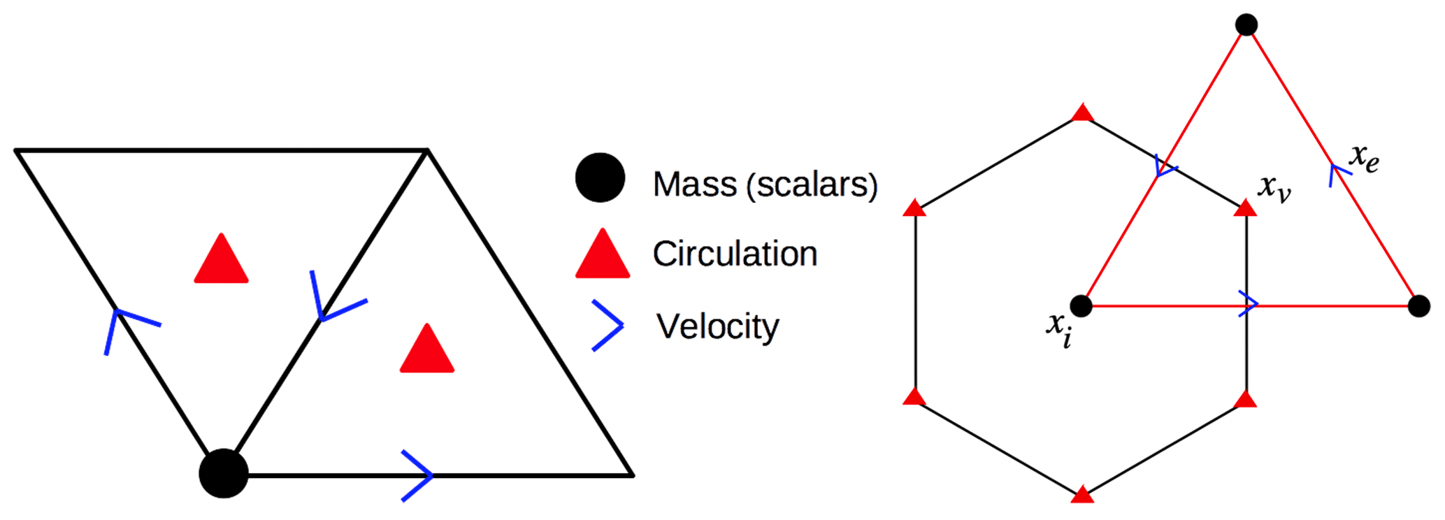
Figure 1 Left: basic computational cell for the icosahedral C-grid discretization, containing one node (for mass and buoyancy), three edges (for velocities) and two triangles (for circulation). Right: relation of the triangular (primal) and hexagonal (dual) cells. Note that the cells are not regular polygons on the sphere and there are 12 exceptional pentagonal dual cells. Separate wavelet transforms are provided for the nodes (scalar-valued) and edges (vector-valued). The adaptive grid consists of the significant nodes and edges, together with nearest neighbours in position and scale necessary for dynamics. The horizontal grid is the same in each vertical layer.

The top vertical layer k=N includes the free surface perturbation with the interface $l=N+\mathrm{1}$ at the free surface, and the bottom vertical interface l=1 is the bathymetry. We include an additional N+1 vertical layer to represent the separate free surface variable η when splitting the baroclinic and barotropic modes. Note that we only store the free surface in the N+1 vertical layer since the depth-integrated fluxes are computed as needed from the other N vertical layers. In the examples we consider here we use a hybrid σ−z grid. The seamount test case uses a Chebyshev vertical grid, while the upwelling and baroclinic jet test cases use a hybrid vertical grid similar to that described in Shchepetkin and McWilliams (2009).

The system (Eqs. 3–5) is a multi-layer rotating shallow water model with inhomogeneous density layers (i.e. δ_iθ_ik≠0) but assumes zero vertical variation of velocity and buoyancy within each layer (i.e. an n−IL⁰ model). A similar model was derived by Ripa (1993) and by Dubos et al. (2015). In this model, to be consistent with the piecewise constant representation of v and θ in the vertical, a vertical average of the horizontal pressure gradient term in each layer is used to compute horizontal velocity (Ripa, 1993).

The Bernoulli function for hydrostatic incompressible flow is

$$\begin{array}{}\text{(6)}& B_{ik}=K_{ik}+{\stackrel{\mathrm{‾}}{{\mathrm{\Phi }}_{il}}}^k+{\displaystyle \frac{{\mathit{\lambda }}_{ik}}{{\mathit{\rho }}_{\mathrm{0}}}},\end{array}$$

where K_ik is the discrete kinetic energy computed from v_ek using appropriate averaging, and Φ_il is the geopotential at vertical layer interfaces l. Pressure λ_ik is calculated by summing the hydrostatic contribution from each vertical layer, g(1−θ_ik)μ_ik, from the top down. The hydrostatic pressure is therefore given by

$$\begin{array}{ll}{\displaystyle }{\mathit{\lambda }}_{ik}& {\displaystyle }=\sum _{j=k}^{N}g(\mathrm{1}-{\mathit{\theta }}_{ij}){\mathit{\mu }}_{ij}-{\displaystyle \frac{\mathrm{1}}{\mathrm{2}}}g(\mathrm{1}-{\mathit{\theta }}_{ik}){\mathit{\mu }}_{ik}\\ {\displaystyle }& {\displaystyle }=\sum _{j=k+\mathrm{1}}^{N}g(\mathrm{1}-{\mathit{\theta }}_{ij}){\mathit{\mu }}_{ij}+{\displaystyle \frac{\mathrm{1}}{\mathrm{2}}}g(\mathrm{1}-{\mathit{\theta }}_{ik}){\mathit{\mu }}_{ik}.\end{array}$$

The terms on the right hand side of Eqs. (3)–(5) are the discretizations of the appropriate Laplacian along-layer diffusion operators, $D_{\mathit{\varphi }}=\mathrm{\nabla }\cdot \left(K_{\mathit{\varphi }}\mathrm{\nabla }\mathit{\varphi }\right)$ (for the scalars) and $D_{\mathit{\delta }}=\mathrm{\nabla }(K_{\mathit{\delta }}\mathrm{\nabla }\cdot v)$ and $D_{\mathit{\omega }}=\mathrm{\nabla }\times (K_{\mathit{\omega }}\mathrm{\nabla }\times v)$ (for the velocity),

$$\begin{array}{}\text{(7)}& {\displaystyle }{D}_{\mathit{\varphi }}={\mathit{\delta }}_i\left(K_{\mathit{\varphi }}{\mathit{\delta }}_e\mathit{\varphi }\right),\text{(8)}& {\displaystyle }{D}_{\mathit{\delta }}={\mathit{\delta }}_e\left(K_{\mathit{\delta }}{\mathit{\delta }}_i\right(v_e\left)\right),\text{(9)}& {\displaystyle }{D}_{\mathit{\omega }}={\mathit{\delta }}_e\left(K_{\mathit{\omega }}{\mathit{\delta }}_v\right(v_e\left)\right).\end{array}$$

The along-layer diffusion coefficients K_ϕ, K_δ and K_ω are constants and can be chosen either to model physical diffusion, or at minimal values to ensure stability. In general K_ϕ=0, although some grid-scale along-layer diffusion on the Lagrangian layer thicknesses μ_ik=ρ₀Δz_ik and buoyancy could be included on the right hand side of Eq. (3) to enhance numerical stability. For better accuracy and stability, mass density (i.e. layer depth) is decomposed into its mean and fluctuating parts and we solve for the fluctuations.

2.2 Vertical remapping and horizontal grid adaptivity

Prognostic variables may be remapped as desired onto a target vertical grid using a conservative piecewise parabolic remapping scheme, as described in Kevlahan and Dubos (2019), to avoid layer collapse or to ensure desired properties of the vertical grid (e.g. approximately isopycnal).

The horizontal grid is adapted on fluctuating pseudo density (i.e. perturbations from mean layer depths), mass-weighted buoyancy and velocities. Adapting on pseudo density ensures that the deformations of the Lagrangian layer interfaces are properly represented by the adaptive grid. Note that if buoyancy is initially constant in each layer, i.e. ${\mathit{\theta }}_{ik}={\stackrel{\mathrm{‾}}{\mathit{\theta }}}_k$, and the vertical grids are not remapped, ${\mathrm{\Theta }}_{ik}=({\stackrel{\mathrm{‾}}{\mathit{\mu }}}_{ik}+{\mathit{\mu }}_{ik}){\stackrel{\mathrm{‾}}{\mathit{\theta }}}_k$; i.e. buoyancy remains constant in each layer.

The horizontal grid adaptation scheme is based on the fact that wavelet coefficients measure the interpolation error at each position and scale. A unique grid point is associated with each wavelet and so removing (small) wavelets from the data structure also removes the corresponding grid point, resulting in an adapted grid.

The essentials of the horizontal grid adaptation strategy are as follows. At the end of a time step the wavelet coefficients of the prognostic variables are computed separately for each horizontal layer. Wavelet coefficients larger than the specified relative tolerance ε for each prognostic variable are retained, and the remainder are deleted. This produces a multiscale adapted grid for each vertical layer. The actual adapted grid is then the union of the adapted grids over all vertical layers. To account for the change in the solution over one time step, nearest neighbours are then added in both scale and position. This is sufficient for a dynamical equation with a quadratic nonlinearity and a time step corresponding to an advective Courant–Friedrichs–Lewy (CFL) criterion of one. Additional points are added to ensure that the adapted grid includes the stencils required for all discrete differential operators. Finally, all variables are inverse wavelet transformed onto the new adapted grid.

The resulting adapted horizontal grid is the same in each vertical layer, which means that the computational elements are a collection of columns of various sizes at each level of resolution j. Full details of the horizontal grid adaptation algorithm are available in Dubos and Kevlahan (2013), Kevlahan and Dubos (2019), and N. K.-R. Kevlahan (2021).

In the incompressible version of wavetrisk described in Kevlahan and Dubos (2019) the grid is adapted after each time step, since the time step is based on the advective CFL number. However, in wavetrisk-ocean the time step is usually significantly smaller than the advective time step, since the advective velocity U≈ 1 m s⁻¹ is much smaller than the barotropic velocity U≈ 200 m s⁻¹. This means that, even in the mode split version (Sect. 3.1), the grid can be adapted much less frequently, leading to a Cpu time saving of about 10 % per time step. For example, in the unstable baroclinic jet case (Sect. 4.3), which uses a barotropic CFL criterion of 35, the grid can be adapted every 8 time steps. This strategy is based on the fact that high resolution is needed primarily to track the fine-scale vorticity filaments and associated density and temperature fluctuations (i.e. the turbulent geostrophic modes).

We use a single time step for all resolution levels j. This may be less efficient than using a resolution-dependent time step in cases where a majority of active grid points are at the finest levels (i.e. low levels of adaptivity), but it greatly simplifies the time-stepping algorithm, especially in the mode split case. We may consider implementing a resolution-dependent Runge–Kutta method (McCorquodale et al., 2015) in future versions of wavetrisk.

3 Numerical scheme

3.1 Barotropic–baroclinic mode splitting time step

The barotropic (or external) mode is typically O(10²) faster than the baroclinic (internal gravity wave) modes and advective timescales of the flow. For an ocean of mean depth H= 4 km the external wave speed is approximately $c_{\mathrm{0}}=\sqrt{gH}\approx$ 200 m s⁻¹, while the typical advective velocity is U≈ 1 m s⁻¹ (the first baroclinic mode is usually much slower, typically $c_{\mathrm{1}}=\frac{c_{\mathrm{0}}}{\mathit{\pi }}\sqrt{-\frac{H}{{\mathit{\rho }}_{\mathrm{0}}}\frac{\mathrm{d}\mathit{\rho }}{\mathrm{d}z}}\approx$ 3 m s⁻¹). To avoid advancing all vertical layers at the very small time step set by the stability criterion for the external modes, most ocean models solve separately the two-dimensional barotropic mode and the three-dimensional baroclinic modes. This barotropic–baroclinic mode separation has been done in three different ways:

1. Imposing a “rigid lid” (no longer used in operational models).

2. Explicit sub-cycling, for example roms (Shchepetkin and McWilliams, 2005), mpas-o (Kang et al., 2021), nemo (Madec and Team, 2015). This involves taking small time steps $\mathrm{\Delta }t\sim \mathrm{\Delta }x/c_{\mathrm{0}}$ for the two-dimensional barotropic mode and longer time steps $\mathrm{\Delta }t\sim \mathrm{\Delta }x/U$ for the baroclinic modes .

3. Using implicit or semi-implicit time-stepping for the free surface (e.g. MITgcm Adcroft et al., 2021). This is the approach we use here.

The implicit free surface filters the fast unresolved wave motions by damping them and does not require an extremely accurate solution of the associated elliptic equation (unlike the rigid lid approach).

The implicit free surface approach has been used in established ocean models such as MITgcm (Marshall et al., 1997; Adcroft et al., 2021), as well as in more recent ocean models such as fesom (Danilov et al., 2017) and mpas-o (Kang et al., 2021). Implicit free surface models are a natural choice for unstructured grid models with variable resolution.

wavetrisk-ocean allows two time-stepping schemes: explicit low-storage RK4 without mode splitting and barotropic–baroclinic mode splitting with a linear implicit free surface. The fully implicit free surface method is unconditionally stable for the barotropic mode, although stability requirements for the baroclinic vertical modes and horizontal geostrophic (vortical) motions limit the practically useful barotropic CFL number. Since the implicit time-stepping scheme is strongly diffusive, the computed free surface waves are strongly diffused at large values of C_barotropic. Therefore, fully implicit mode splitting is appropriate only when we are interested primarily in the slow baroclinic dynamics. However, it does not represent barotropic tides accurately. The following linear free surface scheme shares some features of the barotropic–baroclinic θ step used in MITgcm (e.g. Adcroft et al., 2021, Sect. 2.4).

Because of the significant dissipation associated with the fully implicit method, we implement a θ semi-implicit time integration method, where the parameter $\mathrm{1}/\mathrm{2}\le \mathit{\theta }\le \mathrm{1}$ determines the mix of implicit and explicit approximations of the barotropic flow divergence and surface pressure gradient components. θ=1 gives the full implicit scheme, while $\mathit{\theta }=\mathrm{1}/\mathrm{2}$ gives a Crank–Nicolson scheme (non-dissipative, but less stable). For simplicity, we describe in detail only the fully implicit θ=1 method, using explicit Euler. The general θ method is a simple modification, implemented as in MITgcm (Adcroft et al., 2021, Sect. 2.10.1). Note that the explicit Euler method is unconditionally unstable, and the actual implementation uses third- or fourth-order Runge–Kutta, which are unconditionally stable for θ≥0.75. The stability properties of the time integration scheme is discussed at the end of this section.

Consider a first order discretization of the horizontal equations of motion (for simplicity we have dropped the horizontal indices i, e and have not included the variable porosity used with the penalization). Mass flux through the air–sea interface has been neglected, although it could be included as an extra source term in the top layer.

The first partial explicit Euler step for the scalars is

$$\begin{array}{}\text{(10)}& {\displaystyle }{\mathit{\mu }}_k^{**}={\mathit{\mu }}_k^n-\mathrm{\Delta }t\mathrm{\nabla }\cdot F_k^n,\text{(11)}& {\displaystyle }{\mathrm{\Theta }}_k^{**}={\mathrm{\Theta }}_k^n-\mathrm{\Delta }t\mathrm{\nabla }\cdot \left({\mathit{\theta }}_k^n{F}_k^n\right),\end{array}$$

where $F_k^n={\mathit{\mu }}_k^n{v}_k^n$ is the mass flux in each layer. Because we use Lagrangian vertical coordinates, the layer depths evolve according to Eq. (10), and the two estimates of the depth H+ηⁿ and ${\sum }_{k=\mathrm{1}}^N{\mathit{\mu }}_k^{**}/{\mathit{\rho }}_{\mathrm{0}}$ do not agree exactly. To avoid instability associated with the inconsistent estimates of the free surface position, layer dilation (Bleck and Smith, 1990) is used to stretch each layer slightly to match the free surface estimate ηⁿ. Layer dilation is applied after each partial Euler step to correct the layer depths:

$$\begin{array}{}\text{(12)}& {\mathit{\mu }}_k^{*}={\displaystyle \frac{{\mathit{\rho }}_{\mathrm{0}}(H+{\mathit{\eta }}^n)}{{\sum }_{k=\mathrm{1}}^N{\mathit{\mu }}_k^{**}}}{\mathit{\mu }}_k^{**}.\end{array}$$

After dilating the layers, the mass-weighted buoyancy ${\mathrm{\Theta }}_k^{**}$ is corrected using the new mass density,

$$\begin{array}{}\text{(13)}& {\mathrm{\Theta }}_k^{*}={\displaystyle \frac{{\mathit{\mu }}^{*}}{{\mathit{\mu }}_k^{**}}}{\mathrm{\Theta }}_k^{**}.\end{array}$$

Due to differences between the barotropic and baroclinic mass fluxes, layer dilation conserves global mass but not mass in individual layers. Nevertheless, as Hallberg and Adcroft (2009) pointed out, operational ocean models such as micom and hycom have used this approach successfully. In any case, remapping of vertical layers also mixes buoyancy and inertial mass between layers.

The implicit scheme for the vertical layer velocities and the free surface perturbation equation ${\partial }_t\mathit{\eta }+\mathrm{\nabla }\cdot \left(\right(H+\mathit{\eta }\left)v\right)=\mathrm{0}$ is

$$\begin{array}{}\text{(14)}& {\displaystyle }{v}_k^{n+\mathrm{1}}=v_k^n+\mathrm{\Delta }t(G_k^n-g\mathrm{\nabla }{\mathit{\eta }}^{n+\mathrm{1}}),\text{(15)}& {\displaystyle }{\mathit{\eta }}^{n+\mathrm{1}}={\mathit{\eta }}^n-\mathrm{\Delta }t\mathrm{\nabla }\cdot F^{n+\mathrm{1}},\end{array}$$

where $G_k^n$ is the right hand side of the velocity equation without the external pressure gradient and $F^{n+\mathrm{1}}=\frac{\mathrm{1}}{{\mathit{\rho }}_{\mathrm{0}}}{\sum }_{k=\mathrm{1}}^N{\mathit{\mu }}_k^{n+\mathrm{1}}{v}_k^{n+\mathrm{1}}:=(H+{\mathit{\eta }}^{n+\mathrm{1}})v^{n+\mathrm{1}}$ is the depth-integrated horizontal thickness flux.

Equation (14) is first split into explicit Euler and backwards Euler steps,

$$\begin{array}{}\text{(16)}& {\displaystyle }{v}_k^{*}=v_k^n+\mathrm{\Delta }t{G}_v^n,\text{(17)}& {\displaystyle }{v}_k^{n+\mathrm{1}}=v_k^{*}-\mathrm{\Delta }tg\mathrm{\nabla }{\mathit{\eta }}^{n+\mathrm{1}}.\end{array}$$

We now use Eq. (17) to approximate the depth-integrated horizontal thickness flux as

$$F^{n+\mathrm{1}}\approx F^{*}-\mathrm{\Delta }tg(H+{\mathit{\eta }}^n)\mathrm{\nabla }{\mathit{\eta }}^{n+\mathrm{1}},$$

in Eq. (15), where $F^{*}={\sum }_{k=\mathrm{1}}^N{\mathit{\mu }}_k^{*}{v}_k^{*}/{\mathit{\rho }}_{\mathrm{0}}$. The flux Fⁿ⁺¹ has been linearized about the previous value of the free surface, i.e. ${\mathit{\mu }}_k^{n+\mathrm{1}}\approx {\mathit{\mu }}_k^{*}$ and $(H+{\mathit{\eta }}^{n+\mathrm{1}})\mathrm{\nabla }{\mathit{\eta }}^{n+\mathrm{1}}\approx (H+{\mathit{\eta }}^n)\mathrm{\nabla }{\mathit{\eta }}^{n+\mathrm{1}}$. This gives the linear elliptic equation

$$\begin{array}{}\text{(18)}& {\mathit{\eta }}^{n+\mathrm{1}}={\mathit{\eta }}^n-\mathrm{\Delta }t\mathrm{\nabla }\cdot F^{*}+\mathrm{\Delta }{t}^{\mathrm{2}}\mathrm{\nabla }\cdot \left[g\right(H+{\mathit{\eta }}^n\left)\mathrm{\nabla }{\mathit{\eta }}^{n+\mathrm{1}}\right].\end{array}$$

Rearranging and dividing by Δt² gives

$$\begin{array}{}\text{(19)}& \mathrm{\nabla }\cdot \left[g\right(H+{\mathit{\eta }}^n\left)\mathrm{\nabla }{\mathit{\eta }}^{n+\mathrm{1}}\right]-{\displaystyle \frac{{\mathit{\eta }}^{n+\mathrm{1}}}{\mathrm{\Delta }{t}^{\mathrm{2}}}}=-{\displaystyle \frac{{\mathit{\eta }}^{*}}{\mathrm{\Delta }{t}^{\mathrm{2}}}},\end{array}$$

where we have defined the intermediate free surface

$$\begin{array}{}\text{(20)}& {\mathit{\eta }}^{*}={\mathit{\eta }}^n-\mathrm{\Delta }t\mathrm{\nabla }\cdot F^{*}.\end{array}$$

The adaptive multiscale elliptic solver used to solve Eq. (19) for ηⁿ⁺¹ is described below in Sect. 3.3. Finally, the intermediate layer velocities $v_k^{*}$ are corrected using the backwards Euler step (17) to obtain $v_k^{n+\mathrm{1}}$.

The layer dilation correction is applied once more to ${\mathit{\mu }}_k^{*}$ and ${\mathrm{\Theta }}_k^{*}$, using the new free surface perturbation ηⁿ⁺¹, to obtain ${\mathit{\mu }}_k^{n+\mathrm{1}}$ and ${\mathrm{\Theta }}_k^{n+\mathrm{1}}$. Note that, in contrast to the split-explicit method, a single (slow) barotropic time step $\mathrm{\Delta }t\approx \mathrm{35}\sqrt{gH}$ is used for both the implicit and the explicit steps.

In practice, the explicit Euler steps are incorporated into an explicit RK3 or RK4 scheme (as used in the non-split time integration option). wavetrisk-ocean uses either a third- or fourth-order low storage Runge–Kutta scheme (Kinnmark and Gray, 1984). The RK3 scheme for $y^{\prime }=f\left(y\right)$ is

$$\begin{array}{}\text{(21)}& \begin{array}{rl}{y}^{\mathrm{1}}& =y^n+{\displaystyle \frac{\mathrm{\Delta }t}{\mathrm{3}}}f\left(y^n\right),\\ y^{\mathrm{2}}& =y^n+{\displaystyle \frac{\mathrm{\Delta }t}{\mathrm{2}}}f\left(y^{\mathrm{1}}\right),\\ y^{n+\mathrm{1}}& =y^n+\mathrm{\Delta }tf\left(y^{\mathrm{2}}\right).\end{array}\end{array}$$

This method is third-order accurate for linear terms, second-order accurate for nonlinear terms and stable for a CFL number less than $\sqrt{\mathrm{3}}$. It is well-suited for large, adaptive problems because it uses only one previous time step and has low memory requirements. In a multi-step method like the Runge–Kutta scheme, after each substep the layer dilation correction is applied to the intermediate values of μ_k and Θ_k and the result is interpolated back onto the adapted grid (to ensure mass conservation). The external pressure gradient is neglected in the substeps (it is included in the backwards Euler step 17, which uses the new free surface value ηⁿ⁺¹). We have checked that this time scheme preserves constants (e.g. that in the absence of remapping a constant vorticity or buoyancy field remains constant). Bottom drag and wind stress are implemented as surface fluxes in a separate backwards Euler split step as part of vertical diffusion (see Sect. 3.2).

We finish by presenting the linear stability of the θ method, following the approach of Walters et al. (2009). This analysis specifically addresses the Coriolis term and neglects bottom drag. Figure 2 compares the stable and unstable regions of the θ method in the θ−kcΔt plane for several time integration schemes, where k is the perturbation wavenumber, $c=\sqrt{gH}$ is the external wave speed and Δt is the time step. The explicit Euler and AB2 methods are both unstable for all θ at small wavenumbers, as is RK2 (not shown). In contrast, RK3 and RK4 are both stable for all θ≥0.75. (Note that AB3 is stable for all $\mathit{\theta }>\mathrm{1}/\mathrm{2}$ and is the current preferred choice in MITgcm.) RK3 is actually more stable than RK4 at small k, although this is likely not significant in practice. The results presented below use RK4 with θ=1 (i.e. fully implicit) in Sect. 4.1, 4.2 and RK3 with θ=0.8 in Sect. 4.3.

Figure 2 Neutral linear stability level curves in the θ−ckΔt plane for the θ method for several explicit schemes. The Coriolis parameter $f={\mathrm{10}}^{-\mathrm{4}}$ rad s⁻¹, Δt=360 s. The area above the red curves indicates the stable region for each scheme. Note that RK3 and RK4 are unconditionally stable for all θ≥0.75, while AB2 and explicit Euler are both unstable for small wavenumbers k.

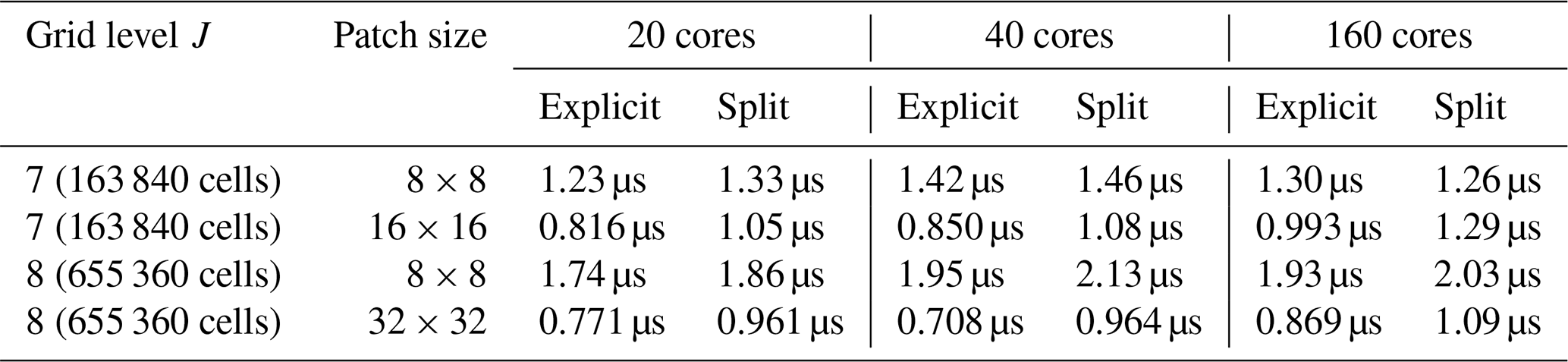
An indication of the maximum computational efficiency of the code is given by the performance of the non-adaptive version. We have performed computations for horizontal grids J=7 (163 840 cells) and J=8 (655 360 cells) with 60 vertical layers for the turbulent baroclinic jet case in Sect. 4.3 without nudging, remapping or diffusion. We show the performance for different choices of patch size p for the hybrid data structure. (Patches are the lowest level of the quad tree and are uniform 2^p×2^p grids.) All runs were performed on the Compute Canada machine niagara with 40-core Intel Skylake nodes, where each node has 202 GB of memory.

Table 1 summarizes the metric τ= (wall clock time × cores) $/$ (iterations × nodes × vertical layers), where iterations = 3 for RK3. For the explicit scheme the best performance is τ≈ 0.8 µs, while for the split time scheme the best performance is τ≈ µs. Since it uses time steps about 45 times larger, the mode split version of the code is about 34–44 times faster than the explicit scheme.

As a comparison with the mode-split case, the best performance of the highly optimized regional ocean model ROMS (Shchepetkin and McWilliams, 2005) is a bit larger than 1 µs (Guillaume Roullet, personal communication, 2019) for realistic configurations, or slightly less than 1 µs with only the dynamical core (as here). (Note that a global model like wavetrisk-ocean has some additional overhead associated with the spherical topology.) Thus, wavetrisk-ocean has roughly similar computational performance to ROMS when run non-adaptively. However, we note that this comparison is not precise, since ROMS solves additional tracer equations and additional computations (e.g. isopycnal diffusion).

Table 1 Computational performance of the explicit and barotropic–baroclinic mode split time schemes without nudging, remapping or diffusion for non-adaptive runs with 60 vertical layers for a modified version of the turbulent baroclinic jet case discussed in Sect. 4.3. Patch size is the size of the uniform patches in the hybrid data structure (i.e. the lowest level of the quad tree). The metric used is (wall clock time × cores) $/$ (iterations × nodes × vertical layers), where iterations = 3 for RK3.

For the 60-vertical-layer case considered here, the mode split scheme adds an overhead of 3 %–30 %. The overhead associated with adaptivity depends on the number of refinement levels, load balancing, how often the grid is adapted, the selected tolerance and the patch size. For a well-balanced case with a grid compression of about 10 times, adaptive runs are about 1.5 times slower per active node than non-adaptive runs on a single grid level (Kevlahan and Dubos, 2019, confirmed for the mode split case). In practice, the performance of realistic, well-balanced, adaptive runs with at least O(10⁶) active nodes is about τ= O(1 µs).

3.2 Vertical diffusion and TKE closure

wavetrisk-ocean implements Laplacian vertical diffusion of buoyancy (i.e. the thermodynamic variable) and velocity in each vertical column as a backwards Euler split step after the main time step. This implicit method is unconditionally stable. The diffusion coefficients of buoyancy and velocity, K_t and K_m, are evaluated either analytically (see the upwelling test case Sect. 4.2) or using an eddy viscosity model with a Kolmogorov-type closure of the TKE. The TKE closure is similar to that used in the nemo ocean model (Madec and Team, 2015, Sect. 10.1.3). TKE is computed dynamically in each vertical column using the one-dimensional equation

$$\begin{array}{}\text{(22)}& {\partial }_t{e}_{il}=K_m\Vert {\partial }_z{v}_{ek}{\Vert }^{\mathrm{2}}-K_t{N}_{il}^{\mathrm{2}}+{\partial }_z\left(K_m{\partial }_z{e}_{il}\right)-c_{\mathit{ϵ}}{\displaystyle \frac{e_{il}^{\mathrm{3}/\mathrm{2}}}{l_{\mathit{ϵ}}}},\end{array}$$

where the TKE e_il is defined at node i and interface $\mathrm{0}\le l\le N$, $N_{il}^{\mathrm{2}}=-g{\mathit{\delta }}_l\left[{\mathit{\rho }}_{ik}\right]/{\mathit{\rho }}_{\mathrm{0}}$ is the local Brunt–Vaisälä frequency squared and l_ϵ is the dissipation length scale. $\Vert {\partial }_z{v}_{ek}{\Vert }^{\mathrm{2}}$ is computed at nodes using the usual wavetrisk formula for kinetic energy applied to ∂_zv_e. The eddy viscosity K_m and eddy diffusivity K_t are then found from the TKE (dropping indices) as

$$\begin{array}{}\text{(23)}& \begin{array}{rl}& K_m=max(c_m{l}_{\mathrm{m}}\sqrt{e},K_{\mathrm{m}\mathrm{0}}),\\ & K_t=max(K_m/{\text{Pr}}_t,K_{t\mathrm{0}}),\end{array}\end{array}$$

where c_m=0.1, l_m is the mixing length and K_m0,K_t0 are minimum diffusivities. The Prandtl and Richardson numbers are

$$\begin{array}{}\text{(24)}& {\mathit{Pr}}_t=\left\{\begin{array}{ll}\mathrm{1}& \text{if }\mathit{Ri}<\mathrm{0.2},\\ \mathrm{5}\mathit{Ri}& \text{if }\mathrm{0.2}\le \mathrm{Ri}\le \mathrm{2},\\ \mathrm{10}& \text{if }\mathit{Ri}>\mathrm{2},\end{array}\right.\mathit{Ri}={\displaystyle \frac{N^{\mathrm{2}}}{\Vert {\partial }_{z}v{\Vert }^{\mathrm{2}}+{\mathit{\epsilon }}_s}},\end{array}$$

where ${\mathit{\epsilon }}_s={\mathrm{10}}^{-\mathrm{20}}$ s⁻². The length scales are computed as in nemo from intermediate values l_up and l_dwn to ensure that their maximum vertical gradients are not larger than depth variations. This modifies the initial values from the basic formula

$$l_{\mathrm{m}}=l_{\mathit{ϵ}}=\sqrt{{\displaystyle \frac{e}{max(N^{\mathrm{2}},N_{\mathit{\epsilon }}^{\mathrm{2}})}}},$$

where $N_{\mathit{\epsilon }}^{\mathrm{2}}={\mathrm{10}}^{-\mathrm{20}}$ s⁻². The Dirichlet boundary conditions for TKE are

$$e(z=\mathit{\eta },t)=max(C_{\text{sfc}}\Vert \mathit{\tau }\Vert /{\mathit{\rho }}_{\mathrm{0}},e_{\mathrm{0}}^{\text{sfc}}),e(z=-H,t)=e_{\mathrm{0}},$$

where C_sfc= 67.83, τ is the surface wind stress, $e_{\mathrm{0}}^{\text{sfc}}={\mathrm{10}}^{-\mathrm{4}}$ m² s⁻² and $e_{\mathrm{0}}={\mathrm{10}}^{-\mathrm{6}}/\sqrt{\mathrm{2}}$ m² s⁻². This large value of C_sfc (compared with the usual value of 3.75), together with a modification of the length scale computation, parameterizes the effect of surface wave breaking.

The TKE Eq. (22) is advanced in time from n to n+1 using an implicit backwards Euler step, discretized as,

$$\begin{array}{}\text{(25)}& \begin{array}{rl}{e}_{il}^{n+\mathrm{1}}& =e_{il}^n+\mathrm{\Delta }t\left\{K_m\Vert {\partial }_z{v}_{ek}^n{\Vert }^{\mathrm{2}}-K_t{N}_{il}^{\mathrm{2}}\right\}\\ & +\mathrm{\Delta }t\left\{{\displaystyle \frac{\mathrm{1}}{\mathrm{\Delta }{z}_{il}}}{\mathit{\delta }}_l\left[{\displaystyle \frac{K_m}{\mathrm{\Delta }{z}_{ik}}}{\mathit{\delta }}_k\left[e_{il}^{n+\mathrm{1}}\right]\right]-c_{\mathit{ϵ}}{\displaystyle \frac{\sqrt{e_{il}^n}{e}_{il}^{n+\mathrm{1}}}{l_{\mathit{ϵ}}}}\right\}.\end{array}\end{array}$$

Positivity of TKE is guaranteed by discretizing the buoyancy term implicitly by multiplying it by $e_{il}^{n+\mathrm{1}}/e_{il}^n$ when the source term (the second term on the right hand side) is negative, i.e. the “Patankar trick” (Patankar, 1980). (Note that N² is always evaluated at time step n.) The resulting one-dimensional tridiagonal system is solved using the lapack routine dgtsv.

After the eddy viscosity and eddy diffusivity have been updated, vertical diffusion is applied to the buoyancy and velocity using a backwards Euler split step,

$$\begin{array}{}\text{(26)}& {\displaystyle }{\mathit{\theta }}_{ik}^{n+\mathrm{1}}={\mathit{\theta }}_{ik}^n+{\displaystyle \frac{\mathrm{\Delta }t}{\mathrm{\Delta }{z}_{ik}}}{\mathit{\delta }}_k\left[{\displaystyle \frac{K_t}{\mathrm{\Delta }{z}_{il}}}{\mathit{\delta }}_l\left[{\mathit{\theta }}_{ik}^{n+\mathrm{1}}\right]\right],\text{(27)}& {\displaystyle }{v}_{ek}^{n+\mathrm{1}}=v_{ek}^n+{\displaystyle \frac{\mathrm{\Delta }t}{\mathrm{\Delta }{z}_{ek}}}{\mathit{\delta }}_k\left[{\displaystyle \frac{K_m}{\mathrm{\Delta }{z}_{el}}}{\mathit{\delta }}_l\left[v_{ek}^{n+\mathrm{1}}\right]\right].\end{array}$$

Source terms at the free surface and bottom (e.g. wind stress, bottom friction, heating or cooling) are implemented via the appropriate Neumann (i.e. vertical flux) boundary conditions. Note that surface heat flux boundary conditions for the temperature, $F_T=Q/\left({\mathit{\rho }}_{\mathrm{0}}{c}_p\right)$, becomes $F_{\mathit{\theta }}=Q/\left({\mathit{\rho }}_{\mathrm{0}}{c}_p\right)a_{\mathrm{0}}/{\mathit{\rho }}_{\mathrm{0}}$ using the simple linear equation of state (2) (without salinity or representation of thermobaric and cabbeling effects).

The numerical implementation of vertical diffusion (Eqs. 26, 27) and the associated TKE closure scheme (25) has been verified using two standard one-dimensional test cases: boundary layer thickening (Kato and Phillips, 1969) and free convection (Willis and Deardorff, 1974). In these cases only the vertical diffusion is active, and the code is run at a coarse resolution J=4. In both cases the results matched exactly those produced by nemo using the same TKE closure model.

The current version of wavetrisk-ocean also includes an enhanced buoyancy diffusion option and a solar penetrative flux model, as in nemo (Madec and Team, 2015, Sect. 5.4.2). The nemo model is based on a two-waveband light penetration scheme.

3.3 Adaptive multiscale elliptic solver

The barotropic–baroclinic mode splitting relies on an efficient and sufficiently accurate algorithm for solving the associated two-dimensional elliptic problem (19). The implicit free surface method is computationally efficient since, unlike the rigid lid method, it does not require a very accurate solution for the free surface perturbation η to achieve an accurate representation of the slow baroclinic vertical modes and geostrophic vortical motions. The wavetrisk algorithm provides a natural adaptive multiscale set of approximation subspaces that we can take advantage of in a simple multigrid elliptic solver (Vasilyev and Kevlahan, 2005).

The elliptic equation is first solved to high accuracy on the coarsest grid J_min using bicgstab. A relative residual norm error of 10⁻⁹ (Kang et al., 2021) is achieved in 20–30 iterations with a barotropic CFL condition of 35 (or in 5–10 iterations with a CFL condition of 10). The solution is then prolonged to the next finer level J_min+1 using the standard wavetrisk interpolation operator for scalars, and the solution is improved using 20–60 Jacobi iterations (a larger residual tolerance is sufficient at these finer scales). This process is continued until the solution is obtained on the finest grid. Since there are relatively few active grid points on the finer grids, this simple multiscale elliptic solver is quite fast.

To accelerate the Jacobi iterations we take advantage of the scheduled relaxation Jacobi (SRJ) method (Yang and Mittal, 2014). We use 30 distinct optimal relaxation factors computed for the elliptic Eq. (19) using the Chebyshev–Jacobi variant of SJR (Adsuara et al., 2017). This method reduces the residual error at the finest scales by 6 orders of magnitude about 8 times faster than the standard Jacobi method, with no additional overhead.

3.4 Penalization of lateral boundaries

Kevlahan et al. (2015) introduced a volume penalization to approximate complex multiscale topography for the two-dimensional shallow water equations. This method uses variable porosity ϕ(x) and permeability σ(x) to approximate no-slip boundary conditions in the limit ϕ→0 and σ→0. Solid regions are defined using a mask function χ(x), which equals 1 in solid regions and equals 0 in fluid regions. In practice, the mask is smoothed over a few grid points.

Since penalization defines solid regions implicitly by modifying the equations, it is especially well-suited for complicated geometries in dynamically adaptive methods since the coastal geometry can be refined easily as the local grid resolution changes. This avoids having to restrict the maximum resolution of the geometry or, conversely, carry extremely fine grids along the coast even when not justified by the fluid dynamics. Kevlahan et al. (2015) showed that the error in satisfying the boundary condition is $O\left(\mathit{\alpha }{\mathit{ϵ}}^{\mathrm{1}/\mathrm{2}}\right)$, where α and ϵ are, respectively, the porosity and permeability in the solid regions. Guinot and Soares-Frazao (2006) and Guinot et al. (2018) have developed a similar penalization method for modelling coastal inundation in urban environments (including subgrid-scale modelling of unresolved topography).

Debreu et al. (2020) developed a three-dimensional extension of this volume penalization to represent bottom bathymetry and non-vertical lateral boundaries. However, in the present paper we restrict ourselves to vertical lateral boundaries and represent bathymetry via a hybrid grid that is approximately uniform in z in shallow regions and terrain following in deep regions Shchepetkin and McWilliams (2009). We intend to implement the fully three-dimensional penalization in future work and concentrate here on developing and validating a basic dynamically adaptive barotropic–baroclinic mode splitting global ocean model.

In the results presented here we fix the porosity in the solid α=0.01 and the permeability ϵ=Δt (minimum stable value for an explicit time step). The velocity penalization is applied in a split step, after the main time step, as in Rasmussen et al. (2011).

3.5 Summary of the complete algorithm

We complete the presentation of the wavetrisk-ocean algorithm by briefly summarizing its main steps in Algorithms 1–4.

Algorithm 1 Complete wavetrisk-ocean time-stepping algorithm.

t=0

while t≤T do

Set time step Δt {use strictest of barotropic, baroclinic and advective CFL conditions}

Explicit Runge–Kutta step (Algorithm 2)

Implicit free surface step (Algorithm 3)

Vertical diffusion split step (Sect. 3.2)

Conservative remapping (Engwirda and Kelley, 2016) {every 5–20 time steps}

Wavelet transform cycle (Algorithm 4)

Adapt horizontal grid (Sect. 2.2)

Apply boundary condition penalization (Sect. 3.4)

$t=t+\mathrm{\Delta }t$

end while

Algorithm 2 Explicit Runge–Kutta sub-cycles (see Equation 21). The steps below are repeated three times for RK3 and four times for RK4.

Layer dilation corrections (Equations 12, 13)

Forward Euler step (Equations 10,11,21)

Wavelet transform cycle (Algorithm 4)

Algorithm 3 Implicit free surface correction.

Solve elliptic equation for new free surface (Equation 19, Section 3.3)

Layer dilation corrections (Equations 12, 13)

Backwards Euler step to correct velocity (Equation 17)

Wavelet transform cycle (Algorithm 4)

Algorithm 4 Wavelet transform cycle to ensure that the solution satisfies the relative error tolerance ε on the entire grid.

Compute wavelets of all variables

Zero out wavelets less than threshold ε

Inverse wavelet transform of solution onto adapted grid {conserves energy and mass}

4 Results

In this section we verify wavetrisk-ocean by using it to simulate three test cases: flow over a seamount (Beckmann and Haidvogel, 1993), coastal upwelling and an unstable baroclinic jet (Soufflet et al., 2016). Each of these tests focuses on a specific property of ocean models. The seamount assesses horizontal pressure gradient errors associated with inclined vertical layers. The upwelling case tests the model's ability to reproduce wind-driven coastal upwelling in a periodic channel with stable stratification and steep bathymetry. Finally, the jet shows how well the model can capture the turbulence generated by baroclinic instabilities. In particular, we will be interested in the ability of wavetrisk-ocean's adaptivity to fully capture the complex turbulence structure and its full energy spectrum with a relatively small number of grid points. The jet case also implements the vertical diffusion TKE model described in Sect. 3.2.

It is, however, difficult to present precise, quantitative comparisons with other models. This is in part because wavetrisk-ocean is an intrinsically global model, and most test cases are designed for β- or f plane configurations. But it is also because there are numerous, often undocumented, differences in implementation (e.g. Lagrangian versus Eulerian vertical grids, choice of along-layer diffusion, time integration). Because of this, our primary goal is to show that wavetrisk-ocean produces reasonable, qualitatively correct results for a set of distinct test cases. Each of these three test cases has been adapted for the sphere, although this inevitably involves choices and the resulting configurations cannot be identical to the planar configurations.

A primary objective of the test cases is to determine which aspects of wavetrisk-ocean should be prioritized for improvement, further development or implementation. For example, the seamount test case shows that the simple horizontal pressure gradient discretization inherited from dynamico should be replaced by a more accurate scheme (e.g. Shchepetkin and McWilliams, 2003) to reduce horizontal pressure gradient errors.

The thermodynamic variable is buoyancy and we use a linear equation of state $\mathit{\rho }={\mathit{\rho }}_{\mathrm{0}}-a_{\mathrm{0}}(T-T_a)$ to relate density to temperature. The vertical grid uses Lorenz coordinates and is remapped periodically onto the original grid using a conservative piecewise parabolic interpolation (Engwirda and Kelley, 2016). The seamount case is remapped every time step, the upwelling case is remapped every 20 time steps and the jet case is remapped every 5 time steps. Laplacian along-layer diffusion is used for all test cases.

4.1 Seamount test case

The seamount test case was introduced by Beckmann and Haidvogel (1993) to quantify the horizontal pressure gradient (HPG) errors in a σ vertical coordinate system, where the vertical layers are stretched between the sea floor and the free surface. This test case consists of a tall Gaussian bathymetry profile with a flat density perturbation that decreases exponentially with depth. In σ coordinates the vertical layers are therefore not aligned with the horizontal isopycnals. The axisymmetric bathymetry is defined as

$$\begin{array}{}\text{(28)}& h\left(r\right)=H(\mathrm{1}-D{e}^{-r^{\mathrm{2}}/L^{\mathrm{2}}}),\end{array}$$

with H= 5 km, D=0.9, L= 40 km. The initial density profile with stable horizontal stratification is

$$\begin{array}{}\text{(29)}& \mathit{\rho }\left(z\right)={\mathit{\rho }}_{\mathrm{0}}+\mathit{\delta }\mathit{\rho }{e}^{z/\mathit{\delta }},\end{array}$$

with δ= 500 m and ρ₀= 1000 kg m⁻³. For this configuration the Brunt–Väisälä frequency is defined as

$$N_{\mathrm{0}}^{\mathrm{2}}=-{\displaystyle \frac{g\mathit{\delta }\mathit{\rho }}{{\mathit{\rho }}_{\mathrm{0}}{H}_{\mathrm{0}}}},$$

and the Burger number as

$$S={\displaystyle \frac{N_{\mathrm{0}}{H}_{\mathrm{0}}}{f_{\mathrm{0}}L}}.$$

The original test case was formulated for an f plane approximation. We have extended this test case to the sphere by placing the centre of Gaussian seamount at latitude 43.29^∘ N such that $f={\mathrm{10}}^{-\mathrm{4}}$ s⁻¹. The radius of the planet is a≈ 153 km, its rotation rate Ω= 7.2921 $\times {\mathrm{10}}^{-\mathrm{5}}$ rad s⁻¹, the linear bottom friction is $r_d=\mathrm{3}\times {\mathrm{10}}^{-\mathrm{4}}$ m s⁻¹ and, as in Shchepetkin and McWilliams (2003), the kinematic viscosity is set to the relatively small value ν= 50 m² s⁻¹.

We compare the growth of the spurious velocity for three different stratifications with Burger numbers $S=\mathrm{0.5},\mathrm{1.5},\mathrm{3}$ (corresponding to δρ= −0.0816, −0.735, −3 kg m⁻³). For all cases we use 20 vertical layers and an nonadaptive horizontal grid with fixed resolution level J_min=5 ($\stackrel{\mathrm{‾}}{\mathrm{\Delta }x}=$ 5.75 km) to set the maximum topographic stiffness ratio

$$r_{\max }={\displaystyle \frac{|h_{i+\mathrm{1}}-h_i|}{h_i+h_{i+\mathrm{1}}}}\approx \mathrm{0.21}.$$

This value is close to the maximum value typically allowed in operational models to ensure acceptable HPG error. The vertical grid uses Chebyshev nodes, which concentrate the vertical layers at the free surface and sea floor. The σ type vertical coordinates are $z_k=A_k\mathit{\eta }-B_{k}H$, where $B_k=\frac{\mathrm{1}}{\mathrm{2}}(\mathrm{1}+\cos (\mathit{\pi }k/N\left)\right)$, $k=\mathrm{0},\mathrm{\dots },N$, where $A_k=\mathrm{1}-B_k$. The vertical grid is remapped to the original Chebyshev nodes every time step. A constant longitude slice through the computational grid is shown in Fig. 3 (top) and the corresponding initial stratification is shown in Fig. 3 (bottom). The barotropic CFL number is fixed at C_barotropic=10 for all simulations, corresponding to Δt= 231 s. The baroclinic CFL numbers for the three stratifications are therefore $C_{\mathrm{baroclinic}}=c_{\mathrm{1}}\mathrm{\Delta }t/\mathrm{\Delta }x=$ 0.027, 0.087, 0.17. All simulations are run for 40 d, significantly longer than the 10 d results reported in Beckmann and Haidvogel (1993).

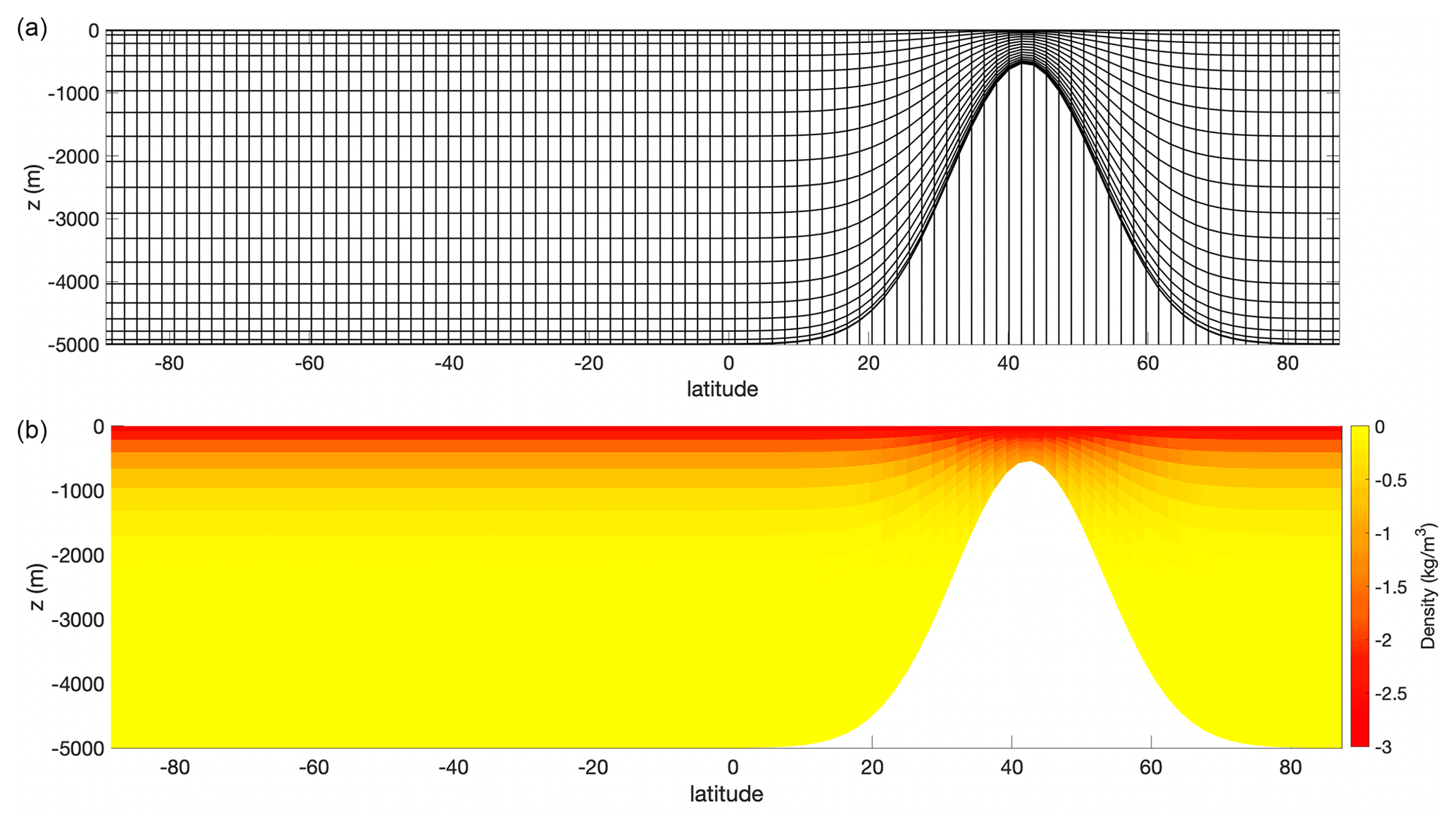
Figure 3 σ-Chebyshev grid (a) and initial stratification (b) for the seamount test case with $\mathit{\delta }\mathit{\rho }=-\mathrm{3}$ kg m⁻³.

Figure 4 Maximum velocity magnitudes (a) and kinetic energies (b) for the seamount test case for three Burger numbers. The maximum topographic stiffness ratio r_max=0.21.

Figure 4 shows that the maximum spurious velocities stabilize at approximately 0.4, 7.7, 28 cm s⁻¹ for Burger numbers S= 0.5, 1.5, 3.0 respectively. We have checked that the spurious velocity magnitudes are similar for the non-split time scheme. In addition to verifying the barotropic–baroclinic splitting algorithm and the incompressible version of the dynamico discretization with the non-adaptive runs, we also confirmed that allowing three levels of grid refinement does not amplify the spurious velocity fields.

The spurious velocity magnitude of 28 cm s⁻¹ at S=3 is about 4 times larger than the results of Debreu et al. (2020), who find a maximum velocity magnitude of about 6.5 cm s⁻¹ with r_max=0.21 using the regional croco model with Δx= 6.7 km. Shchepetkin and McWilliams (2003) found spurious velocities of about 5 cm s⁻¹ using their optimal CubicH scheme. Our value is similar to that reported in Shchepetkin and McWilliams (2003) for the Princeton Ocean Model (POM) density Jacobian type scheme. However, they chose a larger maximum topographic stiffness ratio (0.29 compared to our value of 0.21) and used only 10 vertical layers and Δx= 6.7 km.

Although the standard seamount test case is defined on an f plane, we have placed the seamount at mid-latitudes on the sphere, which would be better approximated by a β plane. Moving the seamount to the North Pole (where β=0) halves the maximum spurious velocity from 28 to 14 cm s⁻¹ at Burger number S=3. This value is only about twice as large as that of the optimal HPG schemes.

Beckmann and Haidvogel (1993) reported maximum velocities of 0.987 cm s⁻¹ (S=0.5), 1.255 cm s⁻¹ (S=1.5) and 1.329 cm s⁻¹ (S=3.0) after 10 d for r_max=0.21 with a stretched horizontal grid. However, they use a different specification of the background density gradient and so we cannot directly compare our results.

Our results suggest that improving the simple discretization of the HPG inherited from dynamico could reduce the HPG error at large Burger numbers.

4.2 Upwelling test case

This is based on the standard ROMS test case contributed by Macks and Middleton. It models wind-driven coastal upwelling and downwelling in a periodic channel with stable stratification. We have adapted the test case to the sphere by considering a zonal channel of width 80 km centred at latitude ϕ₀=45^∘ and maximum depth H= 150 m on a small planet of radius 240 km (see Fig. 5 (right)). The land mass is implemented using volume penalization with porosity $\mathit{\alpha }={\mathrm{10}}^{-\mathrm{6}}$. The parameters for this test case are summarized in Table 2.

Table 2 Parameters for the upwelling test case: reference density ρ₀, Coriolis parameter f₀, gravitational acceleration g, wind stress τ₀, bottom friction r_d, planetary radius a, minimum depth H_min, maximum depth H, channel meridional width L.

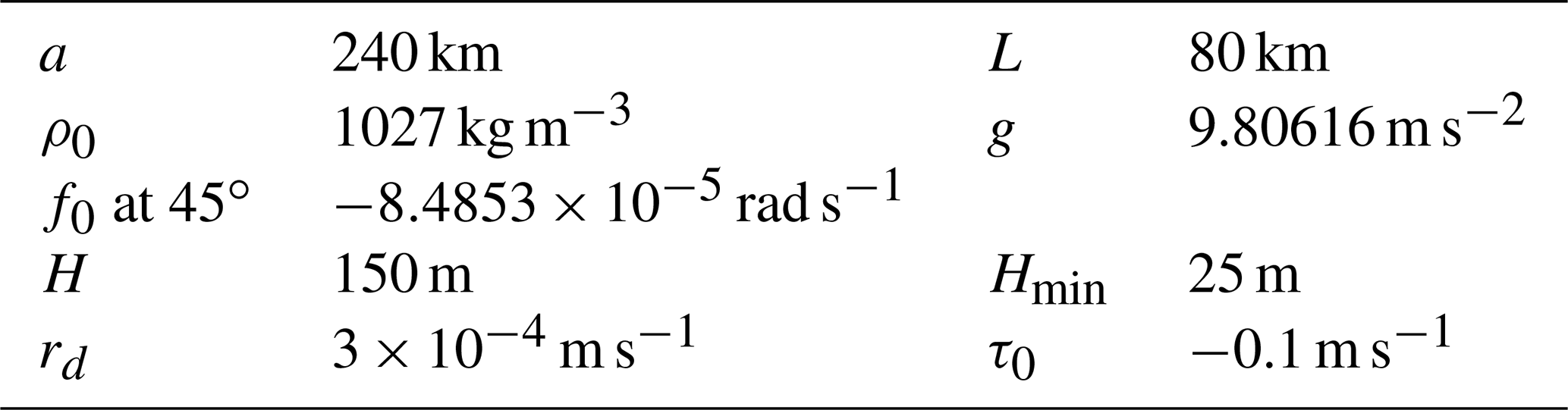
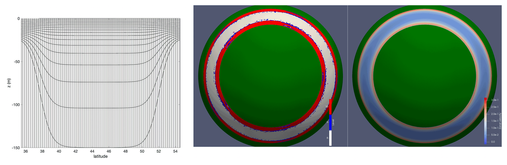
Figure 5 Upwelling test case. Left: vertical grid, with mean horizontal spacing at resolution J=8. Right: horizontal adaptive grid and zonal velocity at day 2 at vertical level 8. The levels $j=\mathrm{8},\mathrm{9},\mathrm{10}$ correspond to mean resolutions $\stackrel{\mathrm{‾}}{\mathrm{\Delta }x}=\mathrm{1},\mathrm{0.5},\mathrm{0.25}$ km.

The profile of the zonal channel is given in terms of latitude ϕ by

$$z\left(\mathit{\varphi }\right)=\left\{\begin{array}{ll}-H+A\left[\mathrm{1}-\tanh \left(\frac{\mathrm{1}}{\mathrm{\Delta }}\left(f\right(y)-\frac{L}{\mathrm{8}})\right)\right],& |\mathit{\varphi }-{\mathit{\varphi }}_{\mathrm{0}}|\le \frac{\mathit{\delta }\mathit{\varphi }}{\mathrm{2}},\\ -H_{\min },& \mathrm{otherwise},\end{array}\right.$$

with

$$f\left(y\right)=\left\{\begin{array}{ll}y& y,\le L/\mathrm{2},\\ L-y,& \mathrm{otherwise},\end{array}\right.$$

with $A=(H-H_{\min })/(\mathrm{1}-\tanh \left(-\frac{L}{\mathrm{8}\mathrm{\Delta }})\right)$, Δ= 5.7 km, $y=\frac{\mathit{\pi }a}{\mathrm{180}}\left(\mathit{\varphi }-({\mathit{\varphi }}_{\mathrm{0}}-\mathit{\delta }\mathit{\varphi })\right)$, channel meridional width $\mathit{\delta }\mathit{\varphi }=L/a\mathrm{180}/\mathit{\pi }\approx \mathrm{19}$^∘. The channel profile is shown in Figs. 5 (left) and 6.

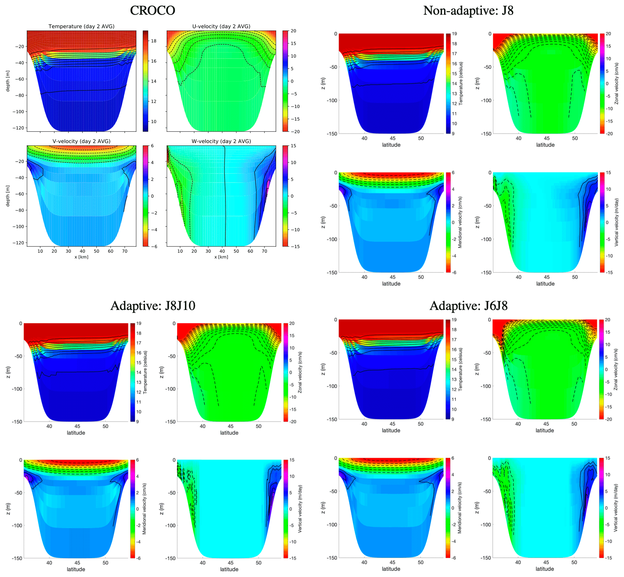
Figure 6 Results for the upwelling test case: zonal averages at day 2. Note that the croco results are for a β plane with zonal channel width of only 20 km.

The vertical grid is hybrid z−σ grid that approximates a uniform in z grid in shallow regions, and at σ grid in deep regions (see Fig. 5 left). This grid is similar to the hybrid grid described in Shchepetkin and McWilliams (2009) and available in NEMO.

The stably stratified temperature profile is given by

$$T\left(z\right)=T_a+\mathrm{4}\tanh \left({\displaystyle \frac{z-z_{\mathrm{0}}}{h_z}}\right)+{\displaystyle \frac{z-z_{\mathrm{1}}}{\stackrel{\mathrm{̃}}{H}}},$$

with T_a=14 ^∘C, h_z= 6.5 m, $z_{\mathrm{0}}=-\mathrm{35}$ m, z₁= −75 m, $\stackrel{\mathrm{̃}}{H}=\mathrm{150}$ m ^∘C⁻¹. Density (and therefore buoyancy) depends on temperature via a linear equation of state

$$\mathit{\rho }\left(z\right)={\mathit{\rho }}_{\mathrm{0}}-a_{\mathrm{0}}\left(T\right(z)-T_a),$$

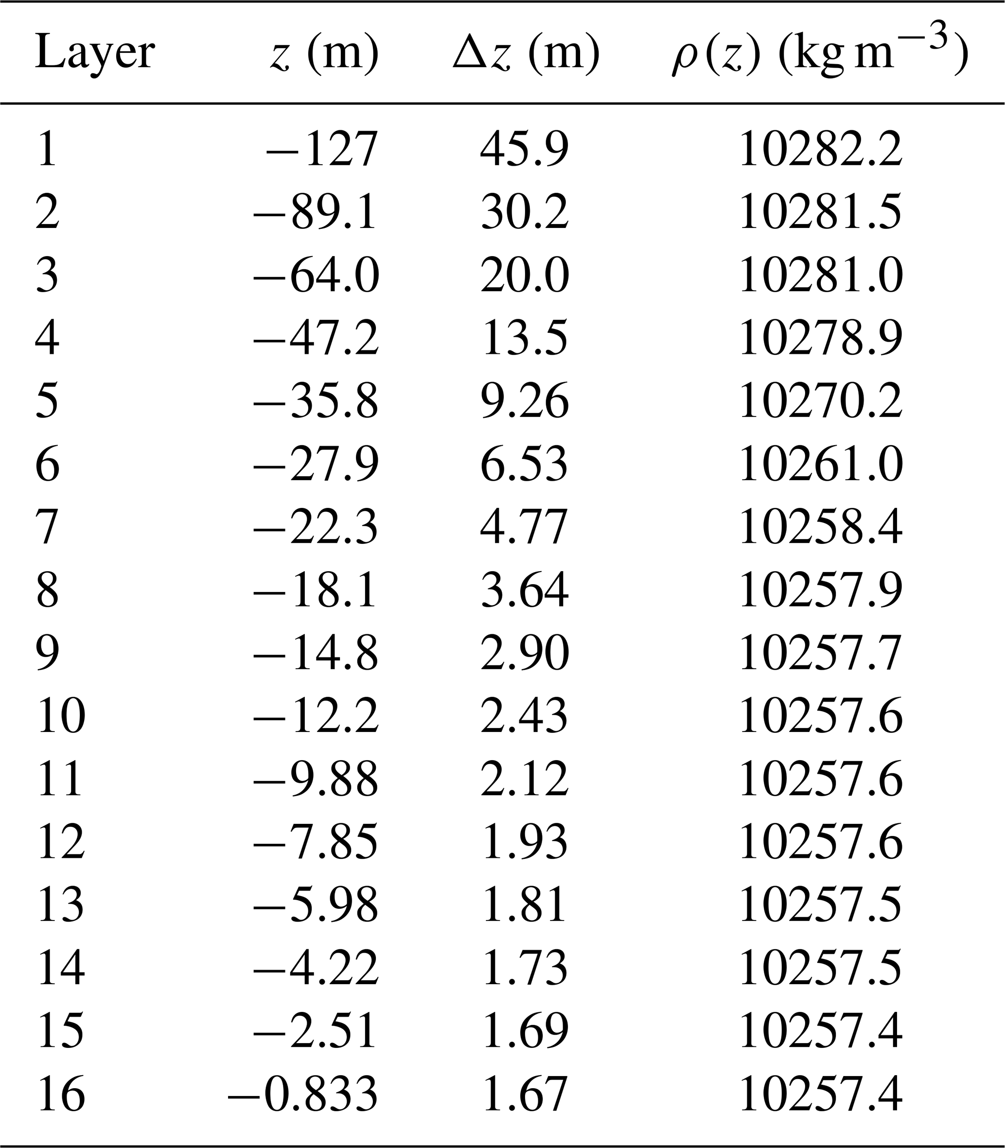
with a₀=0.28 kg m^−3 ∘C⁻¹. The vertical layers and densities in the centre of the channel are given in Table 3.

Table 3 Vertical layers at the centre of the zonal channel: layer centre z, layer thickness Δz and density ρ(z).

Three different simulations were computed: a non-adaptive simulation with resolution J=8 ($\stackrel{\mathrm{‾}}{\mathrm{\Delta }x}=$ 1 km (comparable to the resolution Δx= 1.25 km of the croco benchmark simulation) and two adaptive simulations with resolutions $J=\mathrm{6},\mathrm{7},\mathrm{8}$ (low resolution) and $J=\mathrm{8},\mathrm{9},\mathrm{10}$ (high resolution) with relative tolerance $\mathit{\epsilon }=\mathrm{5}\times {\mathrm{10}}^{-\mathrm{3}}$. The lower resolution adaptive simulation has along-level viscosity 5.5 m² s⁻¹, while the other simulations are run without along-level diffusion. Note that for the low-resolution $J=\mathrm{6},\mathrm{7},\mathrm{8}$ simulation the topographic stiffness ratio r_max=0.66 at the coarsest resolution J=6, which is much larger than the value r_max<0.2 to ensure acceptable pressure gradient error. (A resolution of at least J=8 is required to achieve an acceptable r_max=0.17.) Thus, the low-resolution run verifies the ability of the adaptive code to use much coarser grids than is possible for a non-adaptive code. The high-resolution run tests the ability of the code to provide local high resolution (0.25 km) where needed to achieve more accurate results. The CFL number C_barotropic=35, which corresponds to a time step Δt= 918 s at resolution J=8. The vertical grid is remapped to the initial z−σ grid every 5Δt.

Laplacian vertical diffusion of momentum and temperature is implemented via a backwards Euler implicit split step. The eddy diffusion $K_t={\mathrm{10}}^{-\mathrm{6}}$ m² s⁻¹ is constant and the depth-dependent K_v(x,z) is given by

$$K_v(\mathbf{x},z,t)=K_{\mathrm{0}}\left(\mathrm{1}+\mathrm{4}\exp \left({\displaystyle \frac{z-\mathit{\eta }(\mathbf{x},t)}{H}}\right)\right),$$

where $K_{\mathrm{0}}=\mathrm{2}\times {\mathrm{10}}^{-\mathrm{3}}$ m² s⁻¹ and η(x,t) is the free surface perturbation.

The results are shown in Fig. 6, compared with the benchmark croco simulation on the f plane with $f_{\mathrm{0}}=-\mathrm{8.26}\times {\mathrm{10}}^{-\mathrm{5}}$ s⁻¹. Note that since wavetrisk-ocean uses a Lagrangian vertical grid, we first remap to the initial grid, diagnose vertical velocity from the volume flux Ω through the interfaces, and finally add the component of the pseudo-horizontal velocity in the vertical direction to obtain the true vertical velocity. All results are zonal averages. The wavetrisk-ocean results are qualitatively similar to the croco results, although the maximum zonal velocity is higher (about 34 cm s⁻¹, very similar to the ROMS upwelling test case result, https://www.myroms.org/wiki/UPWELLING_CASE, last access: 22 August 2022). Note that croco uses a split explicit time scheme with a barotropic CFL number of 0.75, much smaller than wavetrisk-ocean's barotropic CFL number of 35. Comparing the non-adaptive J8 results to the adaptive J6J8 results shows that the adaptive code is able to reproduce the main quantitative and qualitative features of a non-adaptive simulation at the highest resolution. This shows that dynamic adaptivity can overcome limitation imposed by the topographic stiffness ratio, r_max<0.2, by using higher resolutions only where the bathymetry gradients are large (see Fig. 5 right). The main difference is that the maximum zonal velocity at low latitudes (lower Coriolis) extends to greater depths.

These results confirm that our code is able to correctly reproduce the physics of coastal upwelling in an idealized configuration, taking into account the differences between simulations on the sphere and on an f plane (variable Coriolis force, much longer zonal channel width, no-slip boundary conditions).

In our final test case, we consider a more realistic baroclinic jet configuration with a more sophistical eddy viscosity model for vertical diffusion, based on a turbulent kinetic energy closure, similar to that used in NEMO.

4.3 Baroclinic jet test case

The final test case assesses the ability of wavetrisk-ocean to simulate submesoscale dynamics. The configuration is a version of the unstable baroclinic jet in a zonal channel proposed by Soufflet et al. (2016), modified for spherical geometry. This test case is designed to include the two dominant mechanisms for generating upper ocean turbulence: surface density stirring by mesoscale eddies and fine-scale instabilities that drive submesoscale turbulence. The original configuration is on a β plane with Coriolis $\mathrm{1.6}\times {\mathrm{10}}^{-\mathrm{11}}$ m⁻¹ s⁻¹. The physical domain on the sphere is a zonally periodic channel of size 500 km by 2000 km with a uniform depth of 4000 m and free slip boundary conditions in the meridional direction. The Rossby deformation radius is ≈ 30 km. The initial density perturbation is zonally invariant, with meridional and depth dependent gradients. The initial velocity is chosen such that it is in geostrophic balance with the density gradient (i.e. integrating upwards, assuming a geostrophic thermal wind balance and zero velocity at the bathymetry). Soufflet et al. (2016) consider four (fixed) grid resolutions, Δx= 20, 10, 5, 2 km, with vertical resolutions of 40, 60, 80 and 100 layers respectively. Since there is no wind stress forcing, energy is maintained by nudging the zonally averaged velocity and density to their initial profiles, with a relaxation time of 50 d.

We have adapted this baroclinic test case to the sphere by considering a small planet of radius a= 1000 km with rotation rate $\mathrm{\Omega }={\mathrm{10}}^{-\mathrm{4}}$ rad s⁻¹, and a zonal channel of meridional width 1000 km centred at 30^∘ N. No-slip boundary conditions are implemented at the channel walls, using the penalization method described in Sect. 3.4. Because wavetrisk-ocean is adaptive, using a relatively large grid J_min=5, Δx_max≈ 38 km, for the coarsest resolution ensures that few grid points are used in the solid (penalized) regions. We allow four levels of grid refinement, $J=\mathrm{6},\mathrm{7},\mathrm{8},\mathrm{9}$, which corresponds to a minimum resolution Δx_min≈ 2.1 km. The simulation uses 60 vertical hybrid layers, ranging in thickness from 430 to 2.5 m at the free surface. The time step Δt=370 s, equivalent to CFL numbers C_barotropic=35 and the maximum C_baroclinic=1.2 (for internal waves). Since the maximum velocity is about 75 cm s⁻¹, the corresponding advective CFL number is about 0.14. In fact, the simulations are stable and the results are very similar for Δt≤630 s.

The Lagrangian vertical grid is remapped every 5Δt to the original hybrid grid, and the horizontal grid is adapted every Δt with a relative tolerance ε=0.02 for all variables. Vertical diffusion is implemented using the TKE closure model described in Sect. 3.2. Along-layer bilaplacian diffusion is included, with viscosities $\mathit{\nu }=\mathrm{2.61}\times {\mathrm{10}}^{\mathrm{8}}$ m⁴ s⁻¹ for the densities and divergent mode, and $\mathit{\nu }=\mathrm{1.63}\times {\mathrm{10}}^{\mathrm{7}}$ m⁴ s⁻¹ for the rotational mode. A small amount of Laplacian diffusion, with viscosity ν=5 m² s⁻¹, is applied to the free surface after the elliptic solution, but before the external pressure gradient correction.

The nudging is implemented by computing the current zonally averaged velocity profiles at the coarsest level J_min=5 and then interpolating the required nudging to each active grid point.

The initial geostrophically balanced density and zonal velocity profiles are shown in Fig. 7. The velocity magnitude is about 3.5 times larger than in Soufflet et al. (2016) due to the more intense horizontal density gradient in the narrower channel. The spherical geometry and longer zonal channel length also mean the results differ quantitatively from Soufflet et al. (2016).

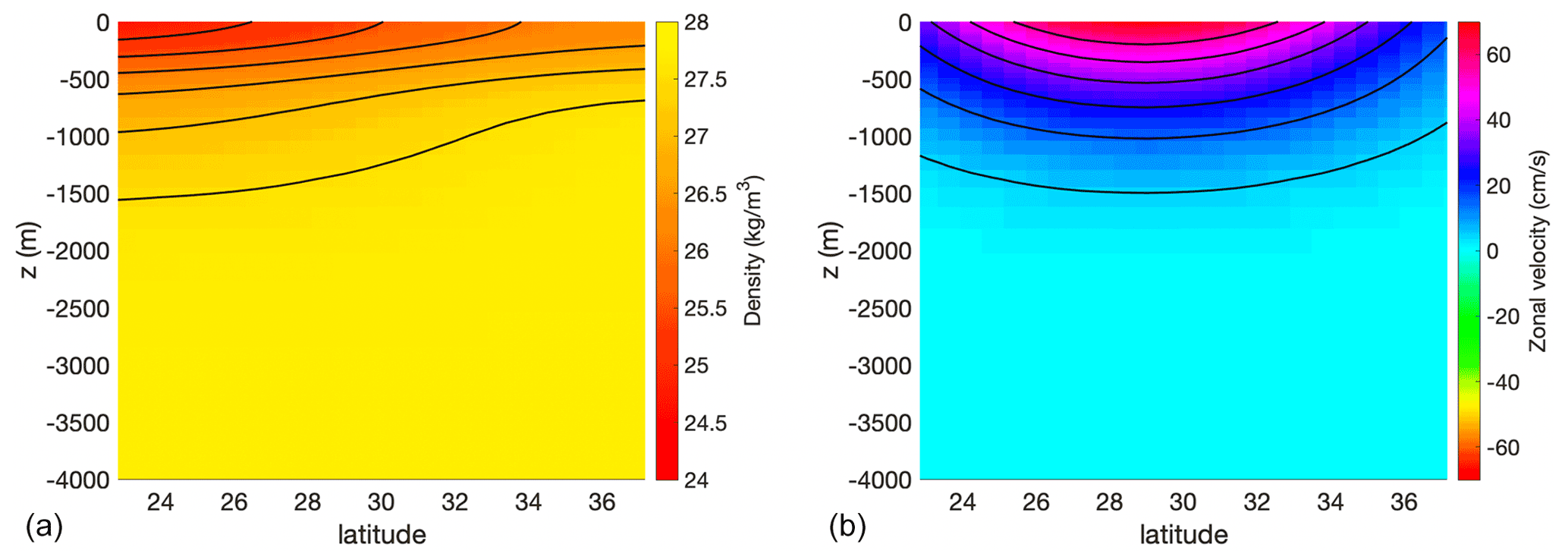
Figure 7 The initial geostrophically balanced density and zonal velocity profiles for the baroclinic jet case. (a) Initial density anomaly ρ−1000 kg m⁻³. Contours at levels 25, 25.5, 26, 26.5, 27, 27.5 kg m⁻³. (b) Zonal velocity. Contours at levels 5, 15, 25, 35, 45, 55 cm s⁻¹.

wavetrisk-ocean was run on 160 cores of the compute canada machine niagara. To spin up, the code was first run non-adaptively at resolution J=5 for 300 d and then restarted from the checkpoint with the four additional adaptive levels and a relative tolerance ε=0.02. Our goal is to have a well-developed turbulent flow to assess the adaptivity and energy spectra, not to compute climate statistics, and so the 20-year run of Soufflet et al. (2016) is not necessary. Since our domain is 12.6 times longer in the zonal direction than the domain used in Soufflet et al. (2016), the ergodic hypothesis could be used to compute statistical quantities using spatial averages instead of temporal averages (provided the flow has reached a statistically stationary state).

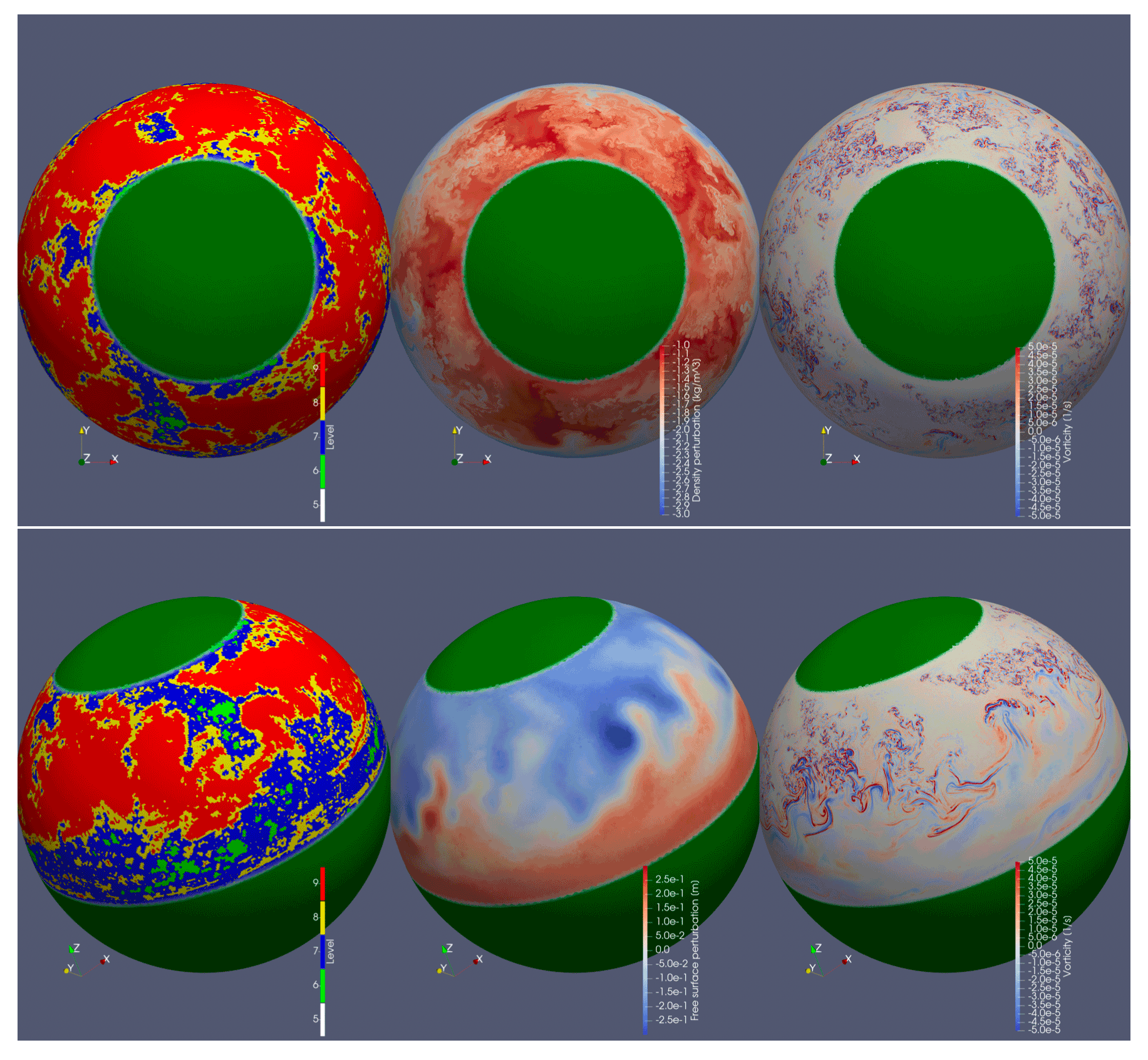
Figure 8 Results of the baroclinic jet test case at 600 d near the surface at depth $z=-\mathrm{1.25}$ m. The coarsest grid is Δx_min≈ 38 km (J=5), and the finest grid is Δx_min≈ 2.1 km (J=9), i.e. four levels of levels of local dyadic refinement. The tolerance is ε=0.02. Top panel (left to right): adaptive grid, density perturbation, relative vorticity. Note that the green regions are the land mass, which are almost entirely at the coarsest level J_min=5, indicated by white in the leftmost figure. Bottom panel (left to right): adaptive grid, free surface perturbation, relative vorticity (note change in scale).

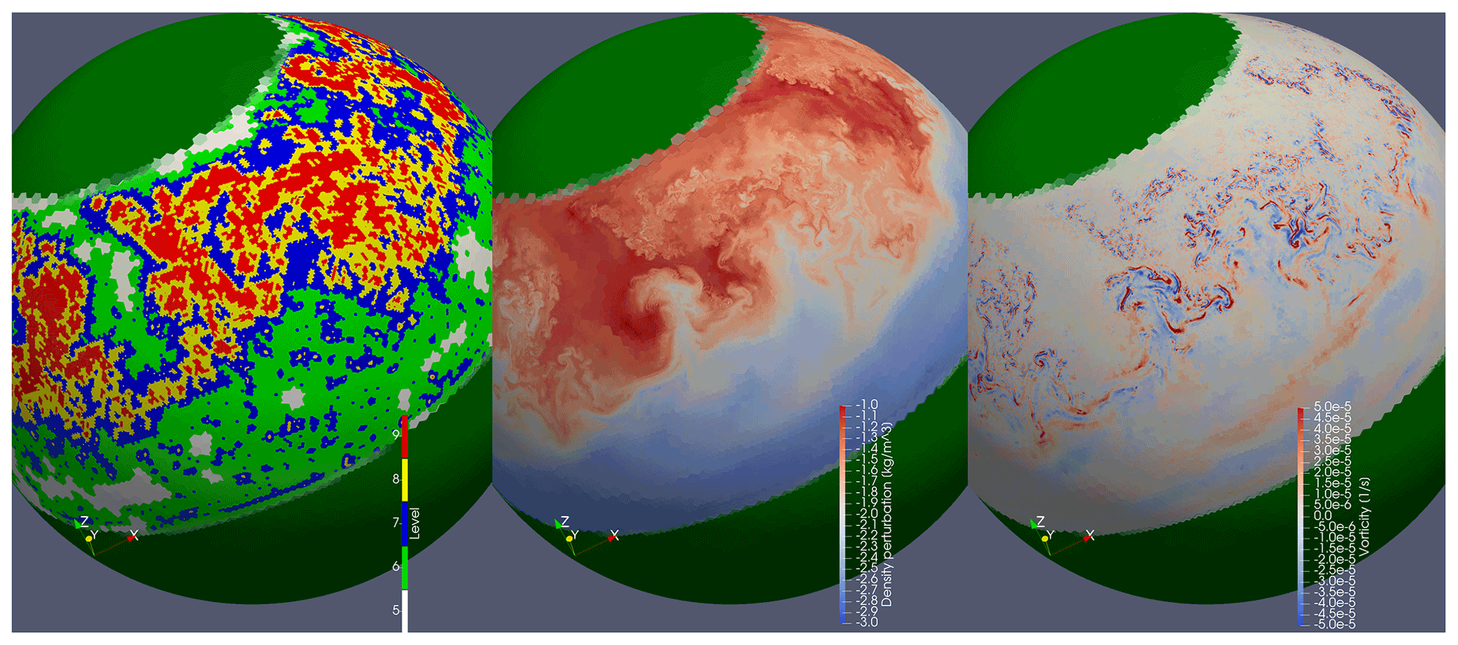
Figure 9 Higher compression run of the baroclinic jet test case with ε=0.06 at 611 d. Adaptive grid (left), density perturbation (centre), relative vorticity (right). Compared with Fig. 8 the grid is more localized, while still capturing the intense vorticity filaments.

Figure 8 shows the adapted grid, density perturbation and relative vorticity near the surface at depth $z=-\mathrm{1.25}$ m at 600 d. The baroclinic jet has become unstable and generates strong submesoscale turbulence. The relatively tolerance is small, ε=0.02, activating the finest resolution in areas of active turbulence. The green (land) regions use the coarsest grid. To illustrate the effect of a larger tolerance, Fig. 9 shows the results with ε=0.06. The grid is far more compressed, with large areas requiring only the coarsest grid. Nevertheless, the more compressed simulation still captures the qualitative fine-scale features of the high-resolution simulation. Overall, the ε=0.06 case uses about half as many grid points than the ε=0.02 case, while still capturing the intense small-scale structures in the density and vorticity fields.

For simplicity, energy spectra are computed from saved vorticity checkpoint data interpolated to fill a fine level of resolution (e.g. J_max or J_max−1). These non-adaptive spherical data on a non-uniform hexagonal grid are then projected onto a uniform longitude–latitude grid of equivalent resolution. The spherical harmonics energy spectrum is then computed from the latitude–longitude data using the spherical harmonics toolbox shtools (Wieczorek and Meschede, 2018). In addition to global energy spectra, shtools also allows the computation of local energy spectra associated with specified sub-regions of the sphere.

Figure 10 shows the spherical harmonic energy spectrum computed from the vorticity field shown in Fig. 8 at depths z=-1.25 and −887 m. The energy spectra are shown as functions of the spherical harmonic wavelength λ, i.e. the equivalent wavelength on the sphere based on the Jeans relation $\mathit{\lambda }=\mathrm{2}\mathit{\pi }a/\sqrt{l(l+\mathrm{1})}$, where l is the degree of the spherical harmonic and a is the radius of the sphere. The wavenumber $k=\mathrm{1}/\mathit{\lambda }$. At the surface, there is a power law range of approximately k⁻² extending over about a decade, from scales of about 25 to 130 km. In contrast, at depth the power law is slightly shallower than k⁻³. The k⁻² power law is typical of baroclinic submesoscale turbulence (e.g. Soufflet et al., 2016; Morvan et al., 2020), while the k⁻³ power is typical of a forward cascade of enstrophy in barotropic turbulence (e.g. Salmon, 1988). The transition between the two types of turbulence occurs between $z=-\mathrm{283}$ and −642 m.

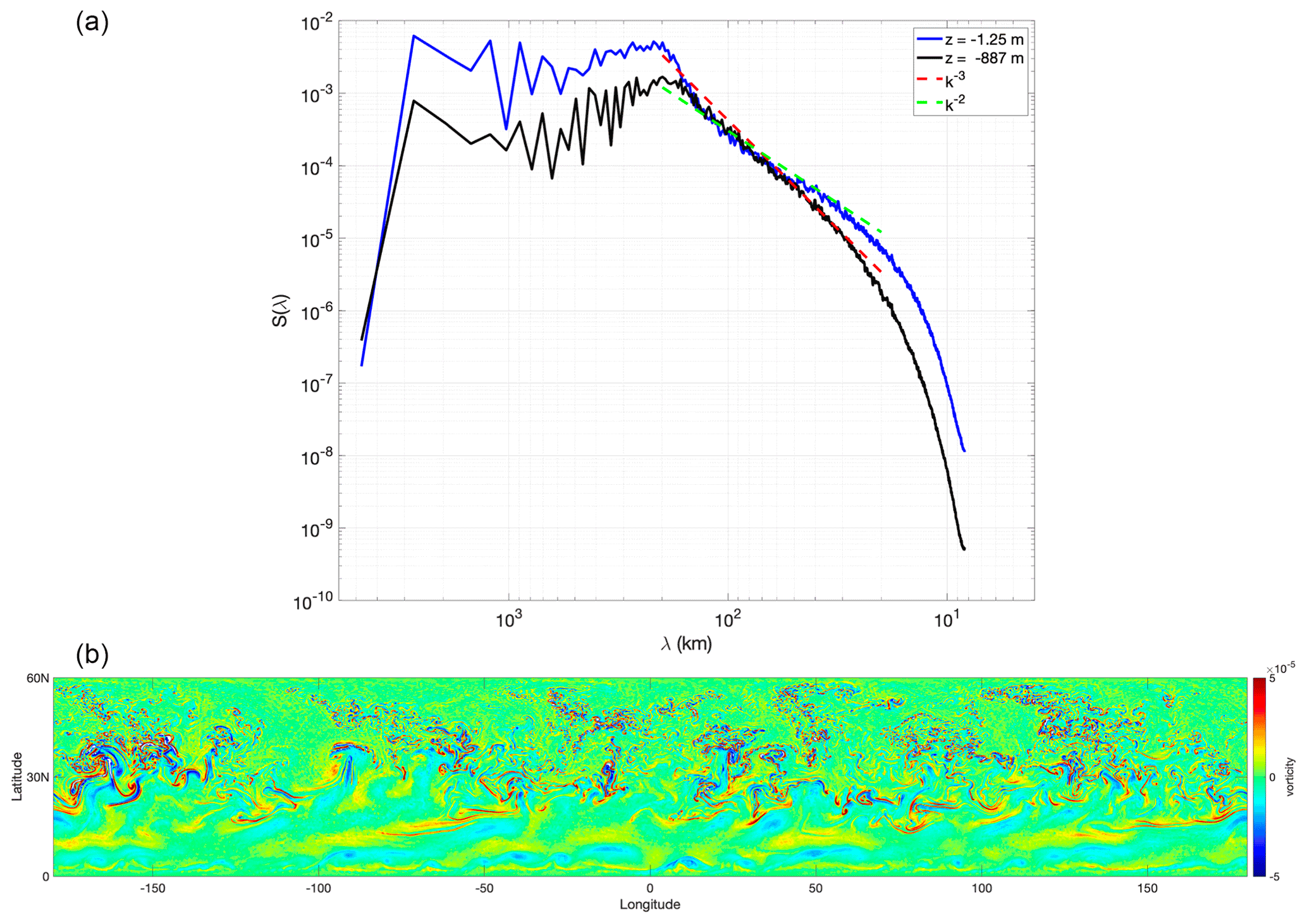
Figure 10 (a) Spherical harmonics energy spectrum for the baroclinic jet test case at 600 d with tolerance ε=0.02 near the surface at depth $z=-\mathrm{1.25}$ m and at a depth of $z=-\mathrm{887}$ m. Near the surface the power law is close to k⁻², while in the interior it is slightly shallower than k⁻³. (b) Latitude–longitude projection of the associated vorticity field at $z=-\mathrm{1.25}$ m in the zonal channel with zonal length 6283 km (at the Equator) and meridional width 1000 km.

5 Conclusions

This paper introduced wavetrisk-2.1, or wavetrisk-ocean, the version of the dynamically adaptive code wavetrisk developed specifically for global ocean modelling. The dynamical equations of wavetrisk-ocean are a multi-layer rotating shallow water model with inhomogeneous density layers, but with no vertical variation of velocity and buoyancy within each layer. This is an n-IL⁰ model in the terminology of Beron-Vera (2021). In such a model, to be consistent with the piecewise constant representation of buoyancy in the vertical, a vertical average of the horizontal pressure gradient term in each layer is used to compute horizontal velocity. For a seamount test case we found that the maximum velocity errors associated with this discretization are about 2–4 times larger than those of state-of-the-art models based on a terrain-following coordinate. This suggests that improving the simple discretization of the horizontal pressure gradient, for example by using the CubicH scheme of Shchepetkin and McWilliams (2003), could reduce the horizontal pressure gradient error. However, since the test case is not completely standardized the comparisons are somewhat imprecise.

Computationally, wavetrisk-ocean uses the same wavelet-based adaptivity approach, hybrid tree–patch data structure and mpi parallelization as wavetrisk.

The main new addition in wavetrisk-ocean is the development of a semi-implicit barotropic–baroclinic mode splitting time step. This relies on a simple and efficient adaptive multigrid elliptic solver and is about 34–44 times faster than an explicit scheme. wavetrisk-ocean also includes conservative remapping using a piecewise parabolic scheme (PPR), vertical diffusion with a turbulent kinetic energy (TKE) closure and volume penalization of horizontal solid boundaries.

We have verified the accuracy and performance of wavetrisk-ocean on three standard test cases: seamount, upwelling and unstable baroclinic jet. In the case of a complex flow such as the unstable baroclinic jet considered here, the adaptive wavetrisk-ocean model achieves physically reasonable results that are qualitatively similar to those of non-adaptive models, but using significantly fewer grid points.

wavetrisk-ocean provides an innovative test bed for exploring the potential of dynamically adaptive methods for ocean modelling. In particular, we are interested in using it to better understand the roles of barotropic and baroclinic dynamics in the production and dissipation of turbulence.

Development priorities for wavetrisk-ocean include implementing a more accurate horizontal pressure gradient discretization, adding vertical adaptivity by optimizing the target grid when remapping (e.g. approximately isopycnal) and using a nonlinear equation of state. Further development will include implementing volume penalization of bathymetry (in addition to coastlines) (Debreu et al., 2020) and investigating more realistic configurations (e.g. with realistic coastline and bathymetry geometry and external forcing). An innovative feature of WAVETRISK-OCEAN is that it could be coupled easily to the WAVETRISK atmosphere model, thus providing a first building block toward an integrated Earth system model using a consistent modelling framework with dynamic mesh adaptivity and mimetic properties.