Representing surface heterogeneity in land–atmosphere coupling in E3SMv1 single-column model over ARM SGP during summertime

The Earth's land surface features spatial and temporal heterogeneity over a wide range of scales below those resolved by current Earth system models (ESMs). State-of-the-art land and atmosphere models employ parameterizations to represent their subgrid heterogeneity, but the land–atmosphere coupling in ESMs typically operates on the grid scale. Communicating the information on the land surface heterogeneity with the overlying atmospheric boundary layer (ABL) remains a challenge in modeling land–atmosphere interactions. In order to account for the subgrid-scale heterogeneity in land–atmosphere coupling, we implement a new coupling scheme in the Energy Exascale Earth system model version 1 (E3SMv1) that uses adjusted surface variances and covariance of potential temperature and specific water content as the lower boundary condition for the atmosphere model. The new lower boundary condition accounts for both the variability of individual subgrid land surface patches and the inter-patch variability. The E3SMv1 single-column model (SCM) simulations over the Atmospheric Radiation Measurement (ARM) Southern Great Plain (SGP) site were performed to assess the impacts. We find that the new coupling parameterization increases the magnitude and diurnal cycle of the temperature variance and humidity variance in the lower ABL on non-precipitating days. The impacts are primarily attributed to subgrid inter-patch variability rather than the variability of individual patches. These effects extend vertically from the surface to several levels in the lower ABL on clear days. We also find that accounting for surface heterogeneity increases low cloud cover and liquid water path (LWP). These cloud changes are associated with the change in cloud regime indicated by the skewness of the probability density function (PDF) of the subgrid vertical velocity. In precipitating days, the inter-patch variability reduces significantly so that the impact of accounting for surface heterogeneity vanishes. These results highlight the importance of accounting for subgrid heterogeneity in land–atmosphere coupling in next-generation ESMs.

1 Introduction

Land surface heterogeneity can influence the atmospheric boundary layer (ABL) dynamics (Bou-Zeid et al., 2020), cloud population (Fast et al., 2019; Chen et al., 2020) and rainfall initiation (Shrestha et al., 2014; Gao et al., 2021) on relatively small spatial and temporal scales. Representing the subgrid-scale heterogeneity of land surface is essential in Earth system models (ESMs) because their typical horizontal grid spacing of about 100 km is insufficient to resolve the variability of land surface characteristics. A common method for representing this surface heterogeneity in land surface models (LSMs) is to introduce “patches” or “tiles” to delineate different land use types, soil characteristics, topographic characteristics (i.e., elevation, slope and aspect), etc., in a model grid box (Koster et al., 2000; Lawrence et al., 2019). Multiple pre-defined patches (e.g., naturally vegetated land, human-managed cropland, urban and lake) may be present within any given grid cell to collectively summarize the land surface characteristics. Recently, emerging schemes have begun to include lateral exchange of water, energy, momentum and carbon among patches, accounting for the effects of those lateral exchanges on the grid-scale features and responses to environmental changes (Chaney et al., 2016, 2018; de Vrese et al., 2016; Lawrence et al., 2019).

Representing the subgrid heterogeneity in ESMs is not limited to the land component. It is in the atmosphere component as well. In the US Department of Energy's Energy Exascale Earth system model version 1 (E3SMv1; Golaz et al., 2019), the E3SM atmosphere model version 1 (EAMv1; Rasch et al., 2019) utilizes Cloud Layers Unified By Binormals (CLUBB; Golaz et al., 2002; Larson et al., 2002; Larson and Golaz, 2005; Bogenschutz et al., 2013) for subgrid atmospheric heterogeneity in turbulent mixing, shallow convection and cloud macrophysics. In addition, CLUBB predicts higher-order moments required for the closure of the model equation system. As documented in Rasch et al. (2019), EAMv1 produces improved climatology compared to the previous-generation ESMs, even though the model exhibits common and long-standing cloud biases that might be related to deficiencies in the cloud, turbulence and convection parameterizations (Xie et al., 2018; Brunke et al., 2019; Zhang et al., 2019).

While both the land and atmosphere models employ parameterizations to represent their spatial heterogeneity, the two component models in E3SMv1 communicate at a grid scale. They only exchange grid-box averages of states and fluxes between the land and atmosphere models. This coupling approach is common in other ESMs such as the Community Earth System Model version 2 (Danabasoglu et al., 2020), the Goddard Earth Observing System Model version 5 (Borovikov et al., 2019), and the Geophysical Fluid Dynamics Laboratory Climate Model version 4 (Held et al., 2019). Neglecting the subgrid information of the land and atmosphere in their coupling potentially leads to simulation biases (Manrique-Suñén et al., 2013; Clark et al., 2015). Previous studies have demonstrated that the turbulent mixing process is significantly different when the subgrid variability is considered, impacting the simulated mean atmospheric state (Mahrt, 2000; Molod et al., 2003; de Vrese et al., 2016).

The main objectives of this study are to (1) implement a new land–atmosphere coupling scheme in a state-of-the-art ESM to account for the subgrid land surface heterogeneity in land–atmosphere coupling, and (2) assess its impacts on ABL characteristics, clouds and precipitation simulations. This paper is organized as follows. Section 2 introduces the land–atmosphere coupling parameterizations and the single-column model (SCM) configuration. Section 3 presents the comparison of the original coupling parameterization and the new treatment accounting for the subgrid-scale heterogeneity. Section 4 gives a summary of major findings.

2 Methodology

In this study, we implemented a new land–atmosphere coupling scheme in E3SMv1 that integrates the information on subgrid-scale heterogeneity to pass on from the E3SM land model (ELM) to EAM. The model was configured as an SCM Bogenschutz et al., 2020) for simulations at the Atmospheric Radiation Measurement (ARM) Southern Great Plain (SGP) site (36.61^∘ N, 97.49^∘ W) during summertime.

2.1 Land–atmosphere coupling in E3SM

In ELM, spatial land surface heterogeneity is represented as a nested subgrid hierarchy in which the highest level is the grid cell while the lowest level is referred to as patch. Following Bogenschutz et al. (2020), the results presented in this study are based on the ne4np4 grid, which corresponds to approximately 7.5^∘ × 7.5^∘ grid spacing. Over SGP, the grid comprises eight patches as listed in Table 1. Increasing horizontal resolution to ne30np4 (approximately 1.5^∘ × 1.5^∘ grid spacing) changes the subgrid surface variability in terms of the composition of the land patches (Table S1), but the SCM results are consistent with those derived from ne4np4 (Figs. S2–S6, the related discussion will be given in Sect. 3.1).

The patches are designated to capture the geophysical and biogeochemical differences between broad categories of land cover and plant functional types within the grid cell. The mean states and fluxes to/from the surface are computed at each patch individually and then aggregated to the grid scale because EAM’s turbulence parameterization CLUBB operates only on grid-cell means. In E3SM, the mass and energy exchanges between land and atmosphere are determined using grid-cell averages of surface properties to serve as the lower boundary conditions. Therefore, the subgrid information on land heterogeneity is lost in the coupling processes, and the state of the atmosphere at the surface is treated as being spatially homogeneous within the grid cell. This default treatment of land–atmosphere coupling is referred to as the “HOM” (homogeneous) method hereafter in this study.

Table 1 Subgrid patches and their respective weights relative to the model grid cell over the ARM SGP site.

^* The patch number is assigned according to the default definition in E3SMv1. Only eight of the pre-defined patches are present in the grid cell over SGP.

In EAM, CLUBB assumes a multivariate, double Gaussian probability density function (PDF) to describe the variability of subgrid liquid water potential temperature (${\mathit{\theta }}_{\mathrm{l}}^{\prime }$), total specific water content ($q_{\mathrm{t}}^{\prime }$), and vertical velocity (w^′), with lower boundary conditions provided by ELM. Due to the staggered grid configuration in CLUBB, only the second- and fourth-order moments are required as lower boundary conditions of the atmosphere (Golaz et al., 2002). The fourth-order moment $\stackrel{\mathrm{‾}}{{w^{\prime }}^{\mathrm{4}}}$ is computed as part of the PDF closure scheme at the surface, which will not be discussed in this study. The second-order moments include the turbulent fluxes of momentum ($\stackrel{\mathrm{‾}}{u^{\prime }{w}^{\prime }}$, $\stackrel{\mathrm{‾}}{v^{\prime }{w}^{\prime }}$), heat ($\stackrel{\mathrm{‾}}{w^{\prime }{\mathit{\theta }}_{\mathrm{l}}^{\prime }}$) and moisture ($\stackrel{\mathrm{‾}}{w^{\prime }{q}_{\mathrm{t}}^{\prime }}$), as well as the turbulent variances and covariance of liquid water potential temperature and total specific water content ($\stackrel{\mathrm{‾}}{{{\mathit{\theta }}_{\mathrm{l}}^{\prime }}^{\mathrm{2}}}$, $\stackrel{\mathrm{‾}}{{q_{\mathrm{t}}^{\prime }}^{\mathrm{2}}}$, and $\stackrel{\mathrm{‾}}{{\mathit{\theta }}_{\mathrm{l}}^{\prime }{q}_{\mathrm{t}}^{\prime }}$, respectively). These scalar variances and covariance can be adjusted to account for the spatial heterogeneity that emerges over the land surface. Conventional surface layer similarity theory, a.k.a. Monin–Obukhov similarity theory (MOST), is used in CLUBB to link the surface scalar variances to the corresponding fluxes (adapted from André et al., 1978):

$$\begin{array}{}\text{(1)}& {\displaystyle }\stackrel{\mathrm{‾}}{{{\mathit{\theta }}_{\mathrm{l}}^{\prime }}^{\mathrm{2}}}=c_{\mathrm{1}}{\left({\displaystyle \frac{\stackrel{\mathrm{‾}}{w^{\prime }{\mathit{\theta }}_{\mathrm{l}}^{\prime }}}{u_{*}}}\right)}^{\mathrm{2}},\text{(2)}& {\displaystyle }\stackrel{\mathrm{‾}}{{q_{\mathrm{t}}^{\prime }}^{\mathrm{2}}}=c_{\mathrm{2}}{\left({\displaystyle \frac{\stackrel{\mathrm{‾}}{w^{\prime }{q}_{\mathrm{t}}^{\prime }}}{u_{*}}}\right)}^{\mathrm{2}},\text{(3)}& {\displaystyle }\stackrel{\mathrm{‾}}{{\mathit{\theta }}_{\mathrm{l}}^{\prime }{q}_{\mathrm{t}}^{\prime }}=c_{\mathrm{3}}\left({\displaystyle \frac{\stackrel{\mathrm{‾}}{w^{\prime }{\mathit{\theta }}_{\mathrm{l}}^{\prime }}}{u_{*}}}\right)\times \left({\displaystyle \frac{\stackrel{\mathrm{‾}}{w^{\prime }{q}_{\mathrm{t}}^{\prime }}}{u_{*}}}\right).\end{array}$$

Here the parameters c₁, c₂ and c₃ are set to 0.4, 0.4 and 0.2, respectively; $\stackrel{\mathrm{‾}}{w^{\prime }{\mathit{\theta }}_{\mathrm{l}}^{\prime }}$ and $\stackrel{\mathrm{‾}}{w^{\prime }{q}_{\mathrm{t}}^{\prime }}$ are area-weighted fluxes of heat and moisture, respectively, derived from ELM at grid level. Similarly, the surface velocity scale (u_*) is approximated based on the area-weighted momentum fluxes as follows:

$$\begin{array}{}\text{(4)}& u_{*}^{\mathrm{2}}={\stackrel{\mathrm{‾}}{u^{\prime }{w}^{\prime }}}^{\mathrm{2}}+{\stackrel{\mathrm{‾}}{v^{\prime }{w}^{\prime }}}^{\mathrm{2}}+\mathrm{0.3}\times w_{*}^{\mathrm{2}}.\end{array}$$

The convective velocity w_* is defined as $w_{*}={\left(\frac{g}{T_{\mathrm{0}}}{z}_i\stackrel{\mathrm{‾}}{w^{\prime }{\mathit{\theta }}_{\mathrm{l}}^{\prime }}\right)}^{\frac{\mathrm{1}}{\mathrm{3}}}$ when surface heat flux is positive (i.e., unstable conditions), where g is the gravitational acceleration, T₀ is a reference temperature set to 300 K, z_i is the mixed layer height in André et al. (1978) but it is set to 1 m in CLUBB. Under stable or neutral conditions, $w_{*}=\mathrm{0}$.

It is worth noting that Eq. (4) is insufficient to represent the characteristics of an underlying heterogeneous surface properly. Since MOST is applied for each patch in ELM, the aggregated grid-cell fluxes neglect the subgrid-scale heterogeneity in land–atmosphere coupling. Therefore, the homogeneous treatment of the friction velocity u_* might not be representative of the land surface heterogeneity in the context of land–atmosphere interactions, potentially leading to biases in the lower atmosphere.

2.2 Implementation of the patch-aggregating approach in E3SM

To account for the surface heterogeneity in land–atmosphere coupling, Machulskaya and Mironov (2018) proposed an approach to aggregating the patch characteristics into equivalent grid-cell scalar variances and covariance. Given that MOST is applied for each patch, this representation can thus retain the subgrid-scale heterogeneity of land surface. In this study, we implemented the Machulskaya and Mironov (2018) scheme in E3SM as briefly described below.

The decomposition of a generic variable x into the grid-box mean $\langle \stackrel{\mathrm{‾}}{x}\rangle$, the fluctuation of patch-mean quantities from the grid-cell mean ${\stackrel{\mathrm{‾}}{x}}^{\prime \prime }$, and the sub-patch fluctuation x^s, can be expressed as:

$$\begin{array}{}\text{(5)}& x=\langle \stackrel{\mathrm{‾}}{x}\rangle +{\stackrel{\mathrm{‾}}{x}}^{\prime \prime }+x^s.\end{array}$$

The angle brackets (〈〉) denote the average quantity over the grid cell of a host model and the overline (^–) denotes a mean state over the patch. The double prime (^′′) denotes a deviation of the patch mean from the grid-cell mean. A schematic diagram illustrating the decomposition is given by Fig. 1 from Machulskaya and Mironov (2018). Based on Eq. (5), we obtain the fluctuation of grid-box mean $x^{\prime }=x-\langle \stackrel{\mathrm{‾}}{x}\rangle ={\stackrel{\mathrm{‾}}{x}}^{\prime \prime }+x^s$. Assuming that $\langle {\stackrel{\mathrm{‾}}{x}}^{\prime \prime }\rangle =\mathrm{0}$ by definition and $\stackrel{\mathrm{‾}}{x^s}=\mathrm{0}$ to simplify the discussion, we then find:

$$\begin{array}{}\text{(6)}& \langle x^{\prime }{y}^{\prime }\rangle =\langle \stackrel{\mathrm{‾}}{\left({\stackrel{\mathrm{‾}}{x}}^{\prime \prime }+x^s\right)\left({\stackrel{\mathrm{‾}}{y}}^{\prime \prime }+y^s\right)}\rangle =\langle {\stackrel{\mathrm{‾}}{x}}^{\prime \prime }{\stackrel{\mathrm{‾}}{y}}^{\prime \prime }\rangle +\langle \stackrel{\mathrm{‾}}{x^s{y}^s}\rangle ,\end{array}$$

where x and y represents either θ_l or q_t. The angle brackets denote the area-weighted average. For reference, we list the formulas for computing the aggregated variances and variance of θ_l and q_t:

$$\begin{array}{}\text{(7)}& {\displaystyle }\langle {{\mathit{\theta }}_{\mathrm{l}}^{\prime }}^{\mathrm{2}}\rangle =\mathrm{\Sigma }{f}_i{{\stackrel{\mathrm{‾}}{{\mathit{\theta }}_{\mathrm{l}}}}^{\prime \prime }}_i^{\mathrm{2}}+\mathrm{\Sigma }{f}_i{\stackrel{\mathrm{‾}}{{\mathit{\theta }}_{\mathrm{l}}^{s\mathrm{2}}}}_i,\text{(8)}& {\displaystyle }\langle {q_{\mathrm{t}}^{\prime }}^{\mathrm{2}}\rangle =\mathrm{\Sigma }{f}_i{{\stackrel{\mathrm{‾}}{q_{\mathrm{t}}}}^{\prime \prime }}_i^{\mathrm{2}}+\mathrm{\Sigma }{f}_i{\stackrel{\mathrm{‾}}{q_{\mathrm{t}}^{s\mathrm{2}}}}_i,\text{(9)}& {\displaystyle }\langle {\mathit{\theta }}_{\mathrm{l}}^{\prime }{q}_{\mathrm{t}}^{\prime }\rangle =\mathrm{\Sigma }{f}_i{\stackrel{\mathrm{‾}}{{\mathit{\theta }}_{\mathrm{l}}}}_i^{\prime \prime }{\stackrel{\mathrm{‾}}{q_{\mathrm{t}}}}_i^{\prime \prime }+\mathrm{\Sigma }{f}_i{\stackrel{\mathrm{‾}}{{\mathit{\theta }}_{\mathrm{l}}^s{q}_{\mathrm{t}}^s}}_i,\end{array}$$

where f_i represents the weight of patch i relative to the corresponding grid cell, and the f_i values for every single grid cell sum to one. Given the fact that the liquid water content q_l is negligible at the surface, we adopt the surface specific humidity q and potential temperature θ for computations at individual patches.

In Eqs. (7)–(9), the first term on the right-hand side (rhs) represents the contribution of the aggregated grid variance from inter-patch difference, as it is the variance of the patch means with respect to the grid-cell mean. The different patch means as depicted by the colored bars in Fig. 1 are derived from the grid-cell mean states by applying MOST for each patch which has different physical properties. The second term represents the contribution of the aggregated grid variance from the variance within individual patches (i.e., sub-patch variance is shown as the error bars in Fig. 1) which are related to their respective fluxes according to MOST (refer to Eqs. 1–3) at the patch level. This treatment retains the patch-level characteristics in the land–atmosphere coupling. When aggregating the patch-specific moments into a grid cell, this approach accounts for both the “inter-patch” variability of surface states (i.e., the first term in the rhs of Eq. 7) and the variability of each patch (“patch” variance denoted by the second term in the rhs of Eq. 7). Hence, the surface boundary conditions contain the information that characterizes heterogeneous surface fluxes and mean states.

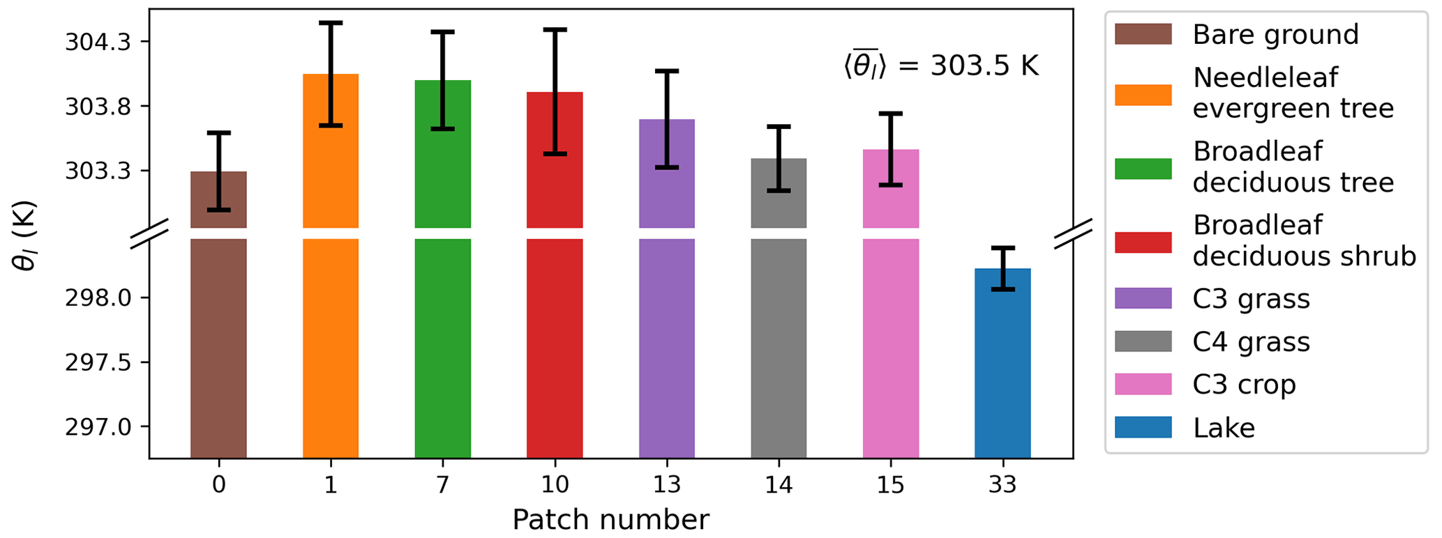
Figure 1 A schematic diagram illustrating the spatial heterogeneity in the grid cell (snapshot at 14:00 LT on 2 June 2015). The vertical bars denote patch-mean liquid water potential temperature θ_l for different patch types shown in colors (grid cell mean is 303.5 K), along with the error bars indicating the MOST-based standard deviation of θ_l and $\sqrt{{\stackrel{\mathrm{‾}}{{\mathit{\theta }}_{\mathrm{l}}^{s\mathrm{2}}}}_i}$, within individual patches. The subgrid-scale variability in the surface states and fluxes are both considered in heterogeneous coupling parameterization.

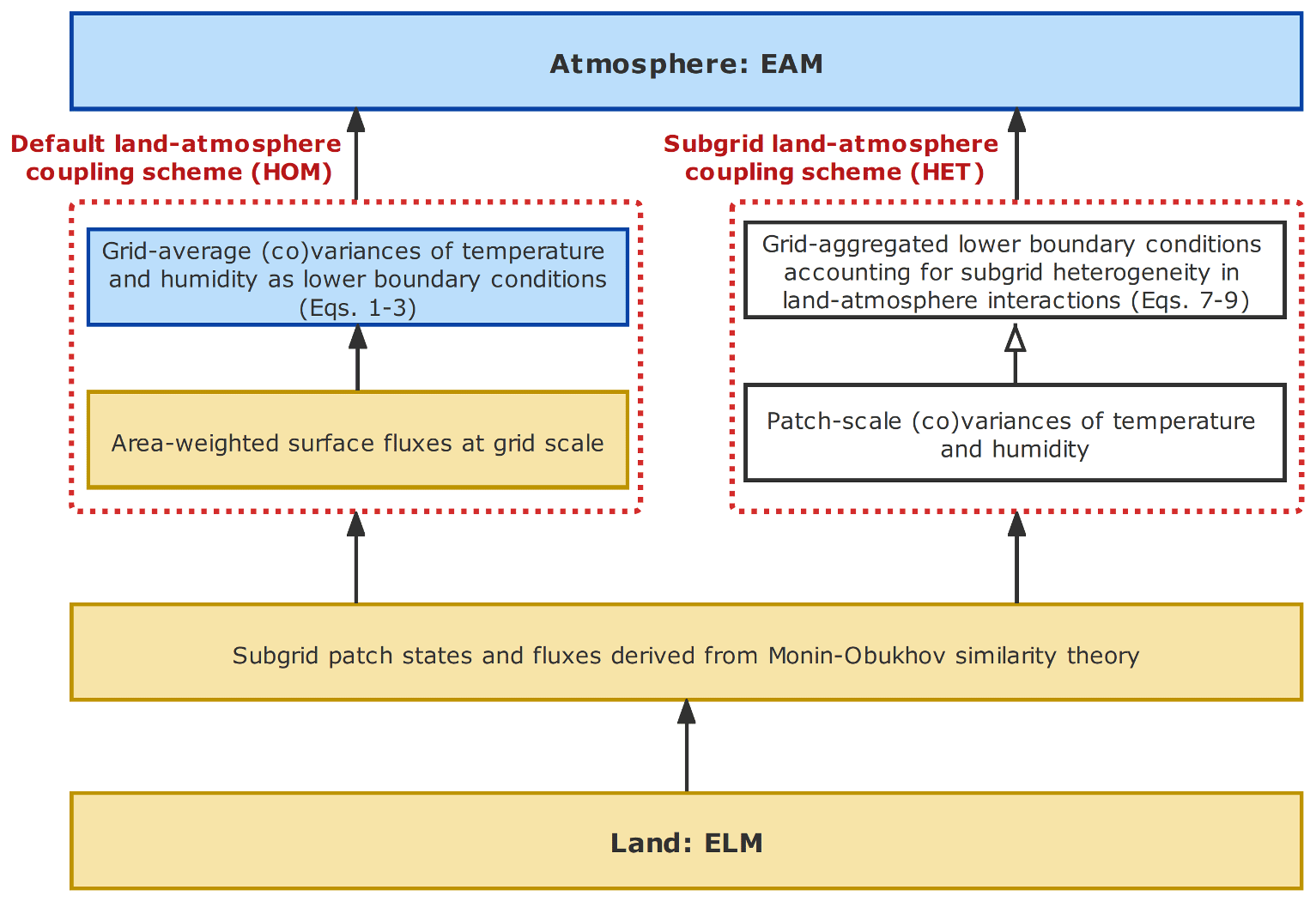
Figure 2 Schematic diagram illustrates the implementation of the default homogeneous (left) and the alternative heterogeneous (right) land–atmosphere coupling in E3SM. The quantities computed in ELM (EAM) are shown in yellow (blue) boxes. The heterogeneous surface moments are computed offline by our implementation (Huang et al., 2021) of the HET approach (white boxes on the right) and then provided to EAM as part of the lower boundary conditions.

2.3 E3SM SCM configurations

We configured the EAMv1 to run at SCM mode with 72 vertical levels over the ARM SGP site. The E3SM SCM has proven to be a useful tool for model development at a low computational cost (Bogenschutz et al., 2020). We performed two simulations from 1 June to 31 August in 2015. The control simulation uses the default E3SM land–atmosphere coupling, which assumes homogeneous land surface, and is labeled as “HOM”. We also configured a “HET” configuration accounting for the land surface heterogeneity in land–atmosphere coupling. In the HET configuration, we used the atmospheric state variables and surface fluxes for each patch in ELM, saved at every model time step from the HOM configuration, to compute the spatially heterogeneous characteristics (i.e., surface variances and covariance of potential temperature and specific water content) following Eqs. (7)–(9) in Sect. 2.2. These heterogeneous surface characteristics were then provided to CLUBB as the lower boundary condition. Figure 2 provides a schematic diagram illustrating how the HOM and HET land–atmosphere coupling approaches are utilized in the E3SM SCM configuration.

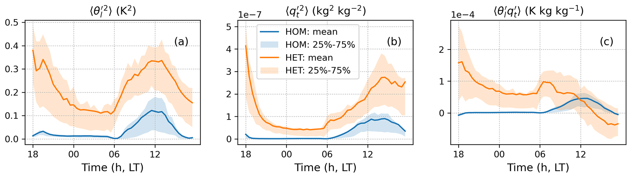
Figure 3 Diurnal cycle of the derived surface properties using HOM and HET approaches in local time (LT), including the variances of (a) liquid water potential temperature $\langle {{\mathit{\theta }}_{\mathrm{l}}^{\prime }}^{\mathrm{2}}\rangle$, (b) total water specific humidity $\langle {q_{\mathrm{t}}^{\prime }}^{\mathrm{2}}\rangle$ and (c) their covariance $\langle {\mathit{\theta }}_{\mathrm{l}}^{\prime }{q}_{\mathrm{t}}^{\prime }\rangle$, which are prescribed based on the ELM output and then passed into CLUBB as the surface boundary conditions. The solid lines denote the seasonal mean quantities and correspondingly the filled areas indicate the 25 % to 75 % quartiles over the period from June to August 2015.

A short-term hindcast approach was applied in order to ensure that the model was well constrained by the large-scale conditions (Ma et al., 2015). The hindcast approach avoids mixing long-term simulation biases with fast errors in physics, allowing us to focus on the effects of different land–atmosphere coupling schemes. During the simulation period, the SCM was initiated every day at 00:00 UTC (18:00 local time (LT)) and run for 48 h. Each simulation's 24 to 48 h forecasts were then combined into a continuous time series for analysis. We note that discontinuity between 2 consecutive days is expected when using the hindcast approach. The initial condition and large-scale forcings (advective tendencies) were from the ARM continuous forcing (Tang et al., 2019; Xie et al., 2004), which is derived from National Oceanic and Atmospheric Administration's (NOAA) Rapid Refresh (RAP) analysis (https://rapidrefresh.noaa.gov/, last access: 19 August 2022) and ARM surface measurements using a constrained variational analysis method (VARANAL Zhang and Lin, 1997). The surface turbulent fluxes from the continuous forcing data were not used in this study since they were computed in ELM.

We evaluated the SCM results against the ARM measurements (Fig. S7). We find that the total cloud fractions in SCM simulations are much higher than the observations (Fig. S7c). The overestimation of clouds leads to decreased surface downwelling of short-wave radiation (not shown). As a result, the model surface sensible heat fluxes decrease, resulting in the bias of near-surface air temperature (Fig. S7a) and the moist biases (Fig. S7b). In Fig. S7d, the observed precipitation peaks in the early morning, whereas the simulated precipitation peaks in the afternoon. This precipitation phase bias in E3SM has been attributed to the model's deficiency in the moist convective parameterization (Xie et al., 2019; Bogenschutz et al., 2020). In the next section, we investigate the impact of accounting for surface heterogeneity in land–atmosphere coupling on clouds, ABL characteristics, and precipitation by contrasting the HOM and HET model simulations.

3 Results

3.1 Surface boundary conditions

Figure 3 shows the diurnal cycle of the surface properties averaged over the simulation period. The discontinuity caused by the hindcast approach is present at 18:00 LT, as expected. We find that the HET configuration produces significantly larger aggregated variances of surface potential temperature ($\langle {{\mathit{\theta }}_{\mathrm{l}}^{\prime }}^{\mathrm{2}}\rangle$) and specific water content ($\langle {q_{\mathrm{t}}^{\prime }}^{\mathrm{2}}\rangle$) than the HOM configuration (Fig. 3a–b). This increase is expected because the HET configuration accounts for the land surface heterogeneity so that the variability of the two scalars increases. Figure 3c shows that the influence of the HET approach on the temperature–humidity covariance ($\langle {\mathit{\theta }}_{\mathrm{l}}^{\prime }{q}_{\mathrm{t}}^{\prime }\rangle$) depends on the time of the day. During the nighttime and early morning, $\langle {\mathit{\theta }}_{\mathrm{l}}^{\prime }{q}_{\mathrm{t}}^{\prime }\rangle$ in HET is significantly larger than that in HOM, which is near zero. The covariance continues to decrease in the morning and eventually becomes negative in the early afternoon.

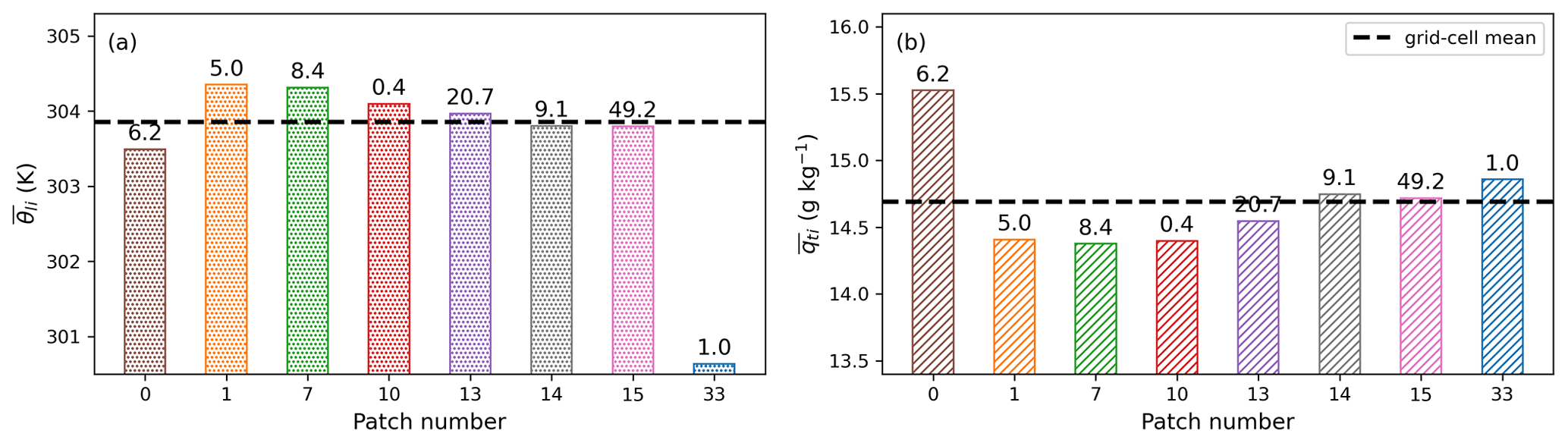
Figure 4 Mean (a) liquid water potential temperature and (b) total water content at 14:00 LT averaged over the study period for each patch within the grid cell of SGP. The color scheme is the same as Fig. 1. The bar label shows the patch weight in % of the grid cell. The dashed black line denotes the grid-cell mean values of θ_l or q_t.

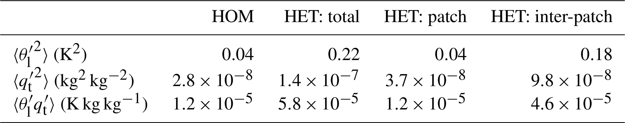
Table 2 summarizes the means of the grid-aggregated surface quantities in HOM, HET and the two components of the HET approach (i.e., the two rhs terms in Eqs. 7–9). We find that the potential temperature variance in HET is 5 times larger than in HOM. Notably, the inter-patch variance (i.e., the first term in rhs of Eq. 7) contributes to 82 % of the increased grid-aggregated variance. Similarly, the specific humidity variance in HET is also 5 times larger than in HOM. The inter-patch variance (i.e., the first term in rhs of Eq. 8) contributes to 70 % of the increase. We also find that the covariance between potential temperature and specific humidity variance in HET is about 4.8 times larger than that in HOM and that the inter-patch covariance (i.e., the first term in rhs of Eq. 9) contributes to 79 % of the increase. These results demonstrate that the inter-patch difference of potential temperature and specific humidity is the primary term driving the differences in surface properties shown in Fig. 3.

Table 2 Patch means of the variances and covariance of temperature and humidity at the surface. This table lists the mean quantities averaged over the JJA season in 2015. The first column (HOM) is derived from the default CLUBB approach using the grid-cell average fluxes provided by ELM. The second column shows the HET-computed surface moments using the subgrid-scale fluxes and states from individual ELM patches. Following Eqs. (7)–(9), the addition of the last two columns is equivalent to the value of the HET: total column​​​​​​​.

We next investigate the negative temperature–humidity covariance $\langle {\mathit{\theta }}_{\mathrm{l}}^{\prime }{q}_{\mathrm{t}}^{\prime }\rangle$ in Fig. 3c. In Fig. 4a that shows the inter-patch variability of surface potential temperature at 14:00 LT when the covariance is at its most negative, we find that the lake (patch no. 33) temperature is significantly lower than the grid-cell mean and contributes the most to the total temperature variance, even though the lake patch only occupies a small fraction of the grid cell (Fig. 5a). In terms of the humidity variance, the vegetated bare ground (patch no. 0) turns into the dominant factor affecting the total humidity variance (Figs. 4b and 5b). Not only these two outstanding patches but also other vegetated patches actually exhibit a negative correlation between temperature and humidity likely due to the rapid evaporation in the afternoon, leading to the negative grid-aggregated temperature–humidity covariance under convective boundary layer conditions.

It is worth noting that even though the initial condition and large-scale forcing are derived from the surface measurements and reanalysis to represent the conditions at the ARM SGP site, there are uncertainties associated with the composition of the land patches. In particular, the fractional coverage of the lake patch might affect the simulation. To address this uncertainty, we performed sensitivity simulations with the lake fractional coverage, increased/decreased by 20 % of its original weight (hereafter named as “lake+” and “lake−”, respectively). We find that the surface scalar variances only slightly increase/decrease in the lake+/lake−​​​​​​​ configurations (see Fig. S1), and the effects do not propagate vertically (Figs. S2–S5). We also compared the model results from HOM and HET using the ne30np4 patch weights as listed in Table S1, and the results are consistent with those derived from ne4np4 (Figs. S2–S6). The impacts of drastically different land patch compositions can be assessed by performing global E3SM simulations with HOM and HET land–atmosphere coupling approaches, which requires further investigation and will be documented in a separate paper.

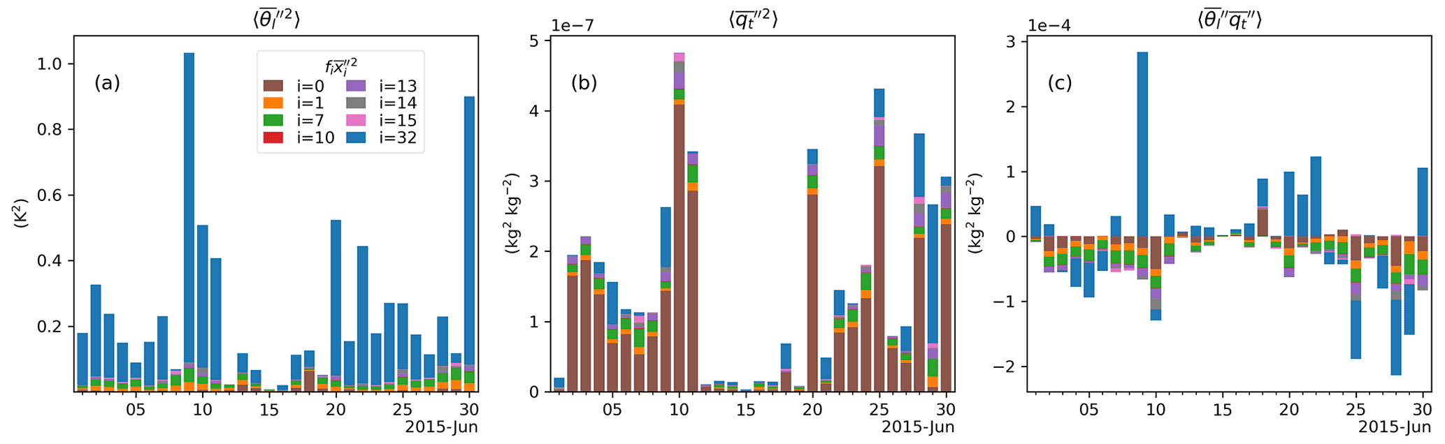
Figure 5 Daily example of the composition of inter-patch variances regarding (a) temperature and (b) humidity, along with the (c) covariance at 14:00 LT using the HET approach. Only the days in June are shown for illustration purposes. The colored bars represent the area-weighted components of the total inter-patch variances in terms of the present patches within the SGP grid cell: 0 – bare ground, 1 – needleleaf evergreen temperate tree, 7 – broadleaf deciduous temperate tree, 10 – broadleaf deciduous temperate shrub, 13 – C₃ non-arctic grass, 14 – C₄ grass, 15 – C₃ crop, 32 – Lake.

3.2 Vertical structure of the atmospheric boundary layer (ABL) on clear-sky days

In this section, we investigate the effects of surface heterogeneity on the ABL characteristics on clear-sky days, when the maximum daytime (06:00–18:00 LT) mean liquid water content below 600 hPa is less than 10⁻³ g kg⁻¹. During the simulation period, there are 17 clear-sky days for this analysis.

The average ABL top on clear-sky days is located at around 830 hPa for SGP during the summer season of analysis (Fig. 6a–b). The simulated ABL structures in HOM and HET are very similar, except that the HET configuration produces a slightly warmer ABL than HOM. In Fig. 6c–d, we find that the increase in the prescribed surface temperature variance and the surface humidity variance in HET propagates upward through the lower half of the ABL. Figure 6e shows that the decrease in temperature–humidity covariance in HET also propagates up towards 920 hPa. The changes in $\stackrel{\mathrm{‾}}{{{\mathit{\theta }}_{\mathrm{l}}^{\prime }}^{\mathrm{2}}}$, $\stackrel{\mathrm{‾}}{{q_{\mathrm{t}}^{\prime }}^{\mathrm{2}}}$ and $\stackrel{\mathrm{‾}}{{\mathit{\theta }}_{\mathrm{l}}^{\prime }{q}_{\mathrm{t}}^{\prime }}$ can further affect the buoyancy term in CLUBB.

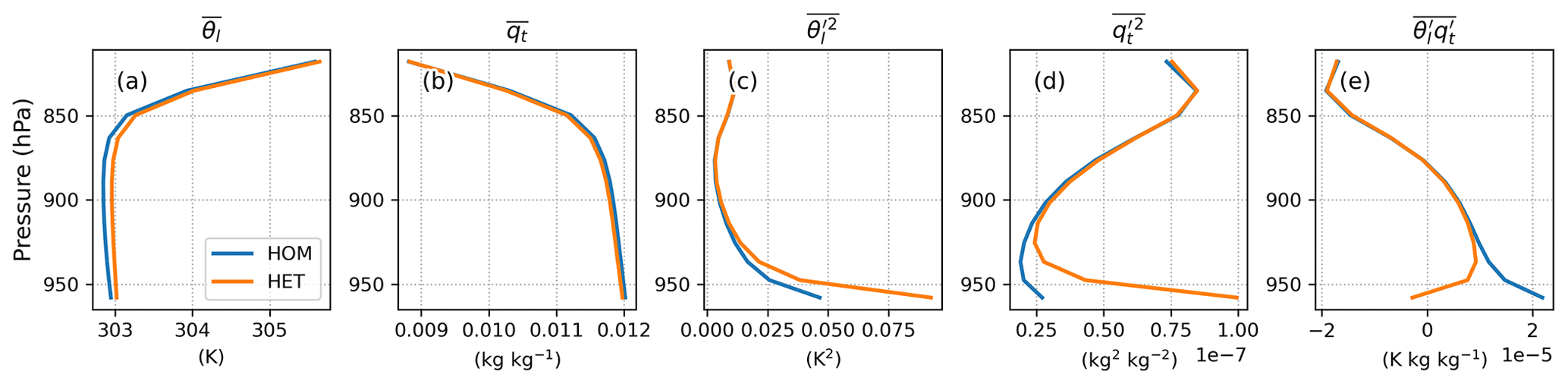
Figure 6 Profiles of CLUBB-predicted (a) liquid water potential temperature θ_l, (b) specific humidity $\stackrel{\mathrm{‾}}{q_{\mathrm{t}}}$, (c) potential temperature variance $\stackrel{\mathrm{‾}}{{{\mathit{\theta }}_{\mathrm{l}}^{\prime }}^{\mathrm{2}}}$, (d) specific humidity variance $\stackrel{\mathrm{‾}}{{q_{\mathrm{t}}^{\prime }}^{\mathrm{2}}}$ and (e) temperature humidity covariance $\stackrel{\mathrm{‾}}{{\mathit{\theta }}_{\mathrm{l}}^{\prime }{q}_{\mathrm{t}}^{\prime }}$ averaged over 14:00–16:00 LT for the clear-sky days. For clarity, the overline for atmospheric quantities hereafter denotes grid-cell mean.

When no cloud is present, the buoyancy production term related to θ_l can be written as

$$\begin{array}{}\text{(10)}& \stackrel{\mathrm{‾}}{{\mathit{\theta }}_{\mathrm{l}}^{\prime }{\mathit{\theta }}_{\mathrm{v}}^{\prime }}=\stackrel{\mathrm{‾}}{{{\mathit{\theta }}_{\mathrm{l}}^{\prime }}^{\mathrm{2}}}+c_{\mathrm{0}}\stackrel{\mathrm{‾}}{{\mathit{\theta }}_{\mathrm{l}}^{\prime }{q}_{\mathrm{t}}^{\prime }},\end{array}$$

where the coefficient $c_{\mathrm{0}}=\frac{\mathrm{1}-{\mathit{ϵ}}_{\mathrm{0}}}{{\mathit{ϵ}}_{\mathrm{0}}}{\mathit{\theta }}_{\mathrm{0}}$ is approximately 200 K. For ${\mathit{ϵ}}_{\mathrm{0}}=R_{\mathrm{d}}/R_{\mathrm{v}}$, R_d is the gas constant of dry air, R_v is the gas constant of water vapor, and θ₀ is a reference temperature. According to Eq. (10), the decrease in $\stackrel{\mathrm{‾}}{{\mathit{\theta }}_{\mathrm{l}}^{\prime }{q}_{\mathrm{t}}^{\prime }}$ would counteract the increase in $\stackrel{\mathrm{‾}}{{{\mathit{\theta }}_{\mathrm{l}}^{\prime }}^{\mathrm{2}}}$ for the buoyancy production of θ_l in HET simulations. However, considering the order of magnitude of the $\stackrel{\mathrm{‾}}{{{\mathit{\theta }}_{\mathrm{l}}^{\prime }}^{\mathrm{2}}}$ term and the $\stackrel{\mathrm{‾}}{{\mathit{\theta }}_{\mathrm{l}}^{\prime }{q}_{\mathrm{t}}^{\prime }}$ term in Fig. 6, we conclude that the buoyancy production term of θ_l is dictated by the $\stackrel{\mathrm{‾}}{{{\mathit{\theta }}_{\mathrm{l}}^{\prime }}^{\mathrm{2}}}$ term. Thus, the buoyancy term $\stackrel{\mathrm{‾}}{{\mathit{\theta }}_{\mathrm{l}}^{\prime }{\mathit{\theta }}_{\mathrm{v}}^{\prime }}$ in HET extends vertically in the lower ABL (Fig. 7a). Furthermore, the increase in HET $\stackrel{\mathrm{‾}}{{\mathit{\theta }}_{\mathrm{l}}^{\prime }{\mathit{\theta }}_{\mathrm{v}}^{\prime }}$ helps to generate the turbulent flux of temperature $\stackrel{\mathrm{‾}}{w^{\prime }{\mathit{\theta }}_{\mathrm{l}}^{\prime }}$ (Fig. 7b), contributing to the production of the upward buoyancy flux (Fig. 7c) and the turbulent kinetic energy (Fig. 7d) in the lower ABL. The enhanced temperature flux thus leads to enhanced vertical mixing and a slightly warmer ABL (Fig. 6a).

Figure 7 Same as Fig. 6, except for the (a) buoyancy production term of θ_l, $\stackrel{\mathrm{‾}}{{\mathit{\theta }}_{\mathrm{l}}^{\prime }{\mathit{\theta }}_{\mathrm{v}}^{\prime }}$, (b) turbulent flux of liquid water potential temperature $\stackrel{\mathrm{‾}}{w^{\prime }{\mathit{\theta }}_{\mathrm{l}}^{\prime }}$, (c) buoyancy flux $\stackrel{\mathrm{‾}}{w^{\prime }{\mathit{\theta }}_{\mathrm{v}}^{\prime }}$, (d) vertical velocity variance $\stackrel{\mathrm{‾}}{{w^{\prime }}^{\mathrm{2}}}$, (e) q_t buoyancy term, $\stackrel{\mathrm{‾}}{q_{\mathrm{t}}^{\prime }{\mathit{\theta }}_{\mathrm{v}}^{\prime }}$, (f) turbulent flux of water specific content $\stackrel{\mathrm{‾}}{w^{\prime }{q}_{\mathrm{t}}^{\prime }}$, (g) third-order moment of vertical velocity $\stackrel{\mathrm{‾}}{{w^{\prime }}^{\mathrm{3}}}$ and (h) skewness of the vertical velocity PDF Sk_w.

Similarly, the q_t-related buoyancy term can be expressed as

$$\begin{array}{}\text{(11)}& \stackrel{\mathrm{‾}}{q_{\mathrm{t}}^{\prime }{\mathit{\theta }}_{\mathrm{v}}^{\prime }}=c_{\mathrm{0}}\stackrel{\mathrm{‾}}{{q_{\mathrm{t}}^{\prime }}^{\mathrm{2}}}+\stackrel{\mathrm{‾}}{{\mathit{\theta }}_{\mathrm{l}}^{\prime }{q}_{\mathrm{t}}^{\prime }}.\end{array}$$

By comparing the magnitude of the two rhs terms in Eq. (11), we find that the buoyancy production term of q_t is more sensitive to the temperature–humidity covariance $\stackrel{\mathrm{‾}}{{\mathit{\theta }}_{\mathrm{l}}^{\prime }{q}_{\mathrm{t}}^{\prime }}$. As shown in Fig. 7e, the HET surface covariance reduces the buoyancy $\stackrel{\mathrm{‾}}{q_{\mathrm{t}}^{\prime }{\mathit{\theta }}_{\mathrm{v}}^{\prime }}$. As a result, the moisture flux, $\stackrel{\mathrm{‾}}{w^{\prime }{q}_{\mathrm{t}}^{\prime }}$, in the lower atmosphere is decreased (Fig. 6f), which partially offsets the upward buoyancy flux enhanced by the buoyancy term of $\stackrel{\mathrm{‾}}{{\mathit{\theta }}_{\mathrm{l}}^{\prime }{\mathit{\theta }}_{\mathrm{v}}^{\prime }}$, as well as the turbulent kinetic energy. Accordingly, there is no significant difference between HOM and HET simulations' surface sensible and latent heat fluxes (not shown). The impact of the HET lower boundary condition does not affect the meteorological states near the surface (e.g., 2 m air temperature, 2 m specific humidity) in this SCM study.

Figure 7g shows that the third-order moment of the subgrid vertical velocity $\stackrel{\mathrm{‾}}{{w^{\prime }}^{\mathrm{3}}}$ is very sensitive to the surface heterogeneity. The $\stackrel{\mathrm{‾}}{{w^{\prime }}^{\mathrm{3}}}$ difference between HOM and HET extends to the entire ABL for the clear-sky days. The budget of $\stackrel{\mathrm{‾}}{{w^{\prime }}^{\mathrm{3}}}$ shows that the source due to buoyancy aloft is increased with heterogeneity in HET simulation, whereas it is partially offset by the decrease in pressure (Fig. 8). In addition, the turbulent advection, which represents vertical transport by updrafts and downdrafts, is also responsible for increasing the HET $\stackrel{\mathrm{‾}}{{w^{\prime }}^{\mathrm{3}}}$ in the upper ABL. This change of $\stackrel{\mathrm{‾}}{{w^{\prime }}^{\mathrm{3}}}$ indicates that the subgrid vertical velocity characteristics have been altered when accounting for surface heterogeneity, as the skewness of the w^′ PDF, ${\mathrm{Sk}}_w\equiv \stackrel{\mathrm{‾}}{{w^{\prime }}^{\mathrm{3}}}/{\stackrel{\mathrm{‾}}{{w^{\prime }}^{\mathrm{2}}}}^{\mathrm{3}/\mathrm{2}}$, increases throughout the ABL (Fig. 7h). The Sk_w changes can have implications for cloudy days, which will be discussed in the next section.

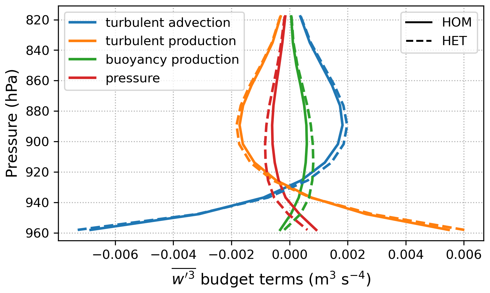
Figure 8 The budget of $\stackrel{\mathrm{‾}}{{w^{\prime }}^{\mathrm{3}}}$ from HOM (solid lines) and HET (dashed lines) configurations, averaged over 14:00–16:00 LT for the clear-sky days.

In summary, with the HET approach applied in E3SM, the diverging patch states play a dominant role in representing the spatial land surface heterogeneity. The HET approach increases the variances of potential temperature and specific water content, as well as their covariance in the nighttime and early morning.

3.3 Impacts of surface heterogeneity on low clouds

In this section, we discuss the impacts of surface heterogeneity on low clouds on non-precipitating cloudy days. A total of 16 d were selected for this analysis when the maximum daytime (06:00–18:00 LT) liquid water content below 600 hPa exceeded 10⁻³ g kg⁻¹ and the daily precipitation rate (convective + large scale) was less than 0.5 mm d⁻¹. The daytime and nighttime (18:00–06:00 LT) averaged cloud properties and cloud liquid water flux profiles are depicted in Fig. 9. We find that the cloud fraction and cloud liquid water content show consistent vertical profiles (Fig. 9a–b). The HET simulation consistently produces more clouds than the HOM simulation. However, the turbulent liquid water flux is insensitive to surface heterogeneity (Fig. 9c).

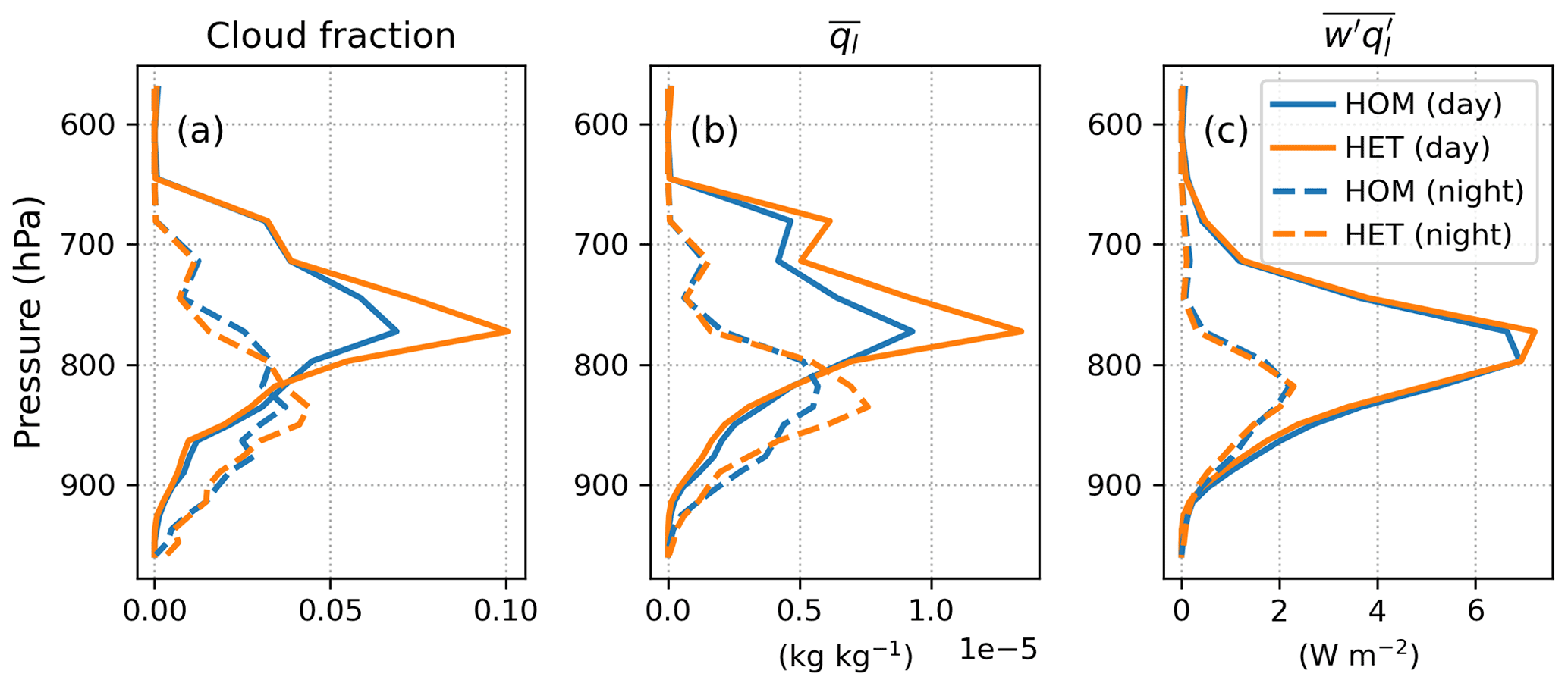
Figure 9 Mean profiles of (a) cloud fraction, (b) cloud liquid water content and (c) liquid water flux averaged during daytime (06:00–18:00 LT in solid lines) and nighttime (18:00–06:00 LT in dashed lines), respectively, over the cloudy days in HOM and HET simulations.

Table 3 Daytime (06:00–18:00 LT) mean, relative difference, and p value from Student t test of liquid water path, ice water path, low cloud fraction, total cloud fraction, net radiation flux, sensible heat flux, and latent heat flux, over the cloudy days in HOM and HET simulations.

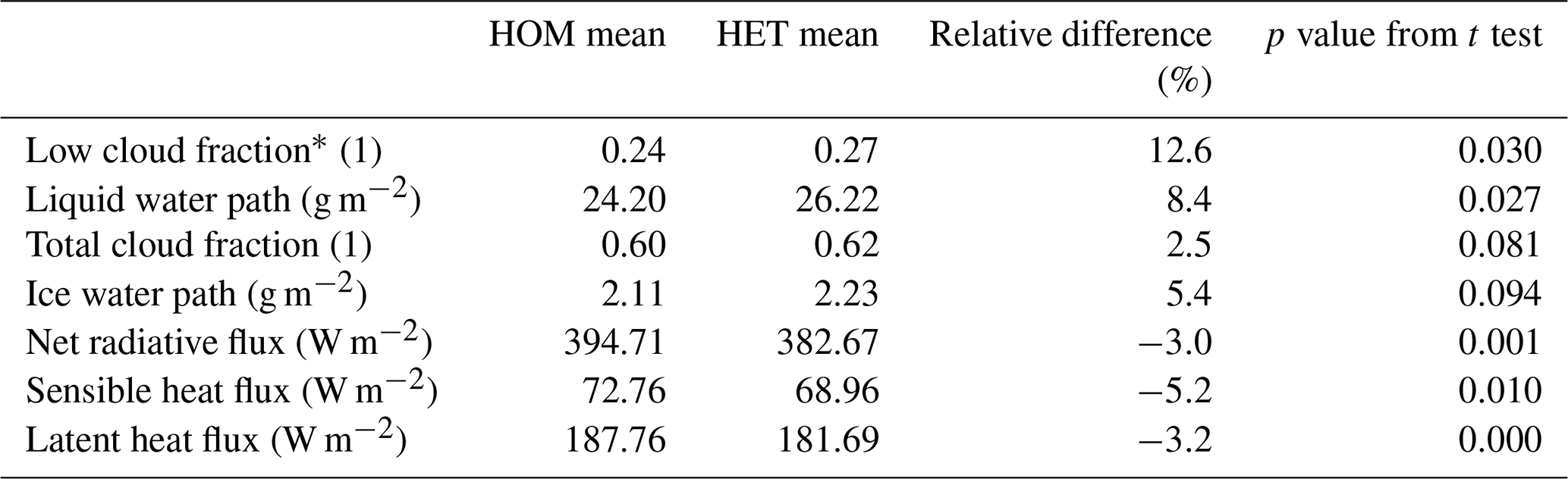
^* The minimum pressure height for low cloud cover is set to 700 hPa in E3SM diagnostics.

Table 3 shows that the HET approach produces a 12.6 % increase in low cloud fraction and an 8.4 % increase in liquid water path compared to the HOM simulation. These differences are found to be statistically significant, with p values of 0.030 and 0.027, respectively. However, the difference in total cloud fraction and ice water path does not pass the Student's t test for statistical significance with a significance level of 0.05. This suggests that accounting for surface heterogeneity in land–atmosphere coupling only affects low clouds in our E3SMv1 SCM configuration. As a result of more low-level clouds in the HET simulation, surface radiative flux as well as sensible and latent heat fluxes are reduced (Table 3).

As the shallow convection mainly occurs in the afternoon over SGP, the vertical profiles averaged over 14:00–16:00 LT on cloudy days are depicted in Fig. 10 for the mean states and variances of θ_l and q_t as well as their covariance. The effects of the HET approach in the sub-cloud layer (below 850 hPa) resemble those on the clear-sky days (Fig. 6). The differences that stemmed from the surface extend vertically to the lower ABL. In cloud layers (between 650 and 850 hPa; see Fig. 9a), the differences in the scalar variances are attributed to the cloud responses to the surface boundary conditions. Similar to the clear-sky days in Sect. 3.2, the turbulent heat flux is increased while the moisture flux is decreased comparably in response to the heterogeneous surface moments, thereby leading to slightly larger buoyancy flux and turbulent kinetic energy at the lower sub-cloud layer. In cloud layers, the differences in turbulent fluxes between HOM and HET configurations are negligible (Fig. 11).

Figure 10 Same as Fig. 6, except for non-precipitating cloudy days. Note that the y axis here spans higher than Fig. 6.

Figure 11 Same as Fig. 7, except for non-precipitating cloudy days.

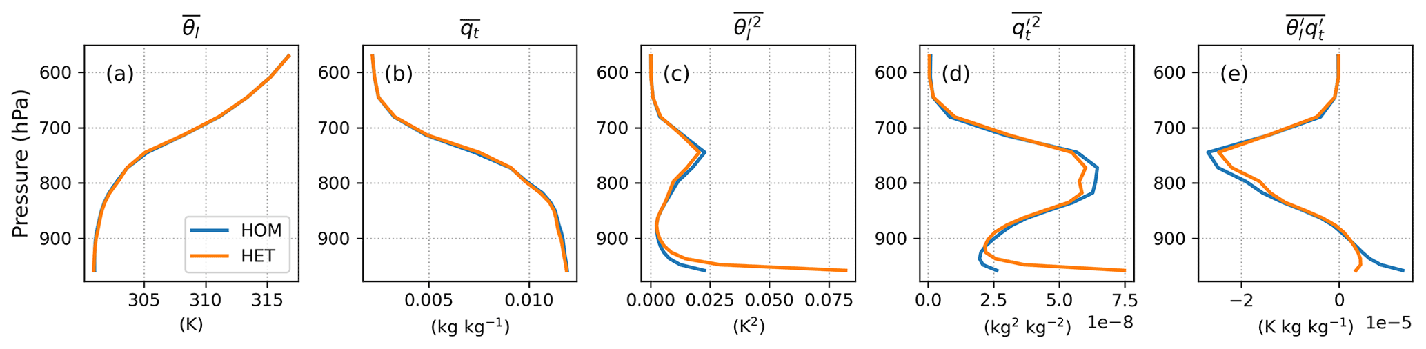
Figure 11h shows that Sk_w increases slightly below clouds and decreases in cloudy layers when accounting for surface heterogeneity. Since low Sk_w indicates symmetric turbulent mixing corresponding to the stratocumulus regime, and high Sk_w indicates the presence of strong updrafts which correspond to the shallow cumulus regime (e.g., Golaz et al., 2002, 2005; Cheng and Xu, 2006; Guo et al., 2014), the differences in Sk_w between HOM and HET indicate a change in the turbulence structure and, consequently, the cloud regime. The decrease in Sk_w within the cloud layers (Fig. 10d) indicate a shift toward a more symmetric mixing within clouds, leading to higher cloud fraction and liquid cloud content, consistent with the findings summarized in Table 3.

3.4 Impacts of surface heterogeneity on precipitation

This section discusses the impacts on precipitation by accounting for surface heterogeneity in land–atmosphere coupling. A total of 50 d in the simulation period were selected for this analysis when the daily precipitation rate (convective + large scale) exceeded 0.5 mm d⁻¹ in both HOM and HET configurations. The results show that the mean precipitation rate in HOM is 6.1 mm d⁻¹, slightly lower than the precipitation rate of 6.4 mm d⁻¹ in HET. This difference, however, does not pass the Student's t test for statistical significance. The diurnal cycle of total precipitation is shown in Fig. 12a. Both HOM and HET simulations produce pronounced diurnal cycle of precipitation, with high precipitation rates in the afternoon, mainly contributed by the convective precipitation (Fig. 12b). The precipitation rate peaks between 12:00 and 14:00 LT in the default HOM simulation. In the HET simulation, the peak time is slightly delayed by about 1 h, but the difference does not pass the statistical significance test. We also find that the differences in precipitation PDF between HOM and HET are minimal (<1 %; see Fig. 13).

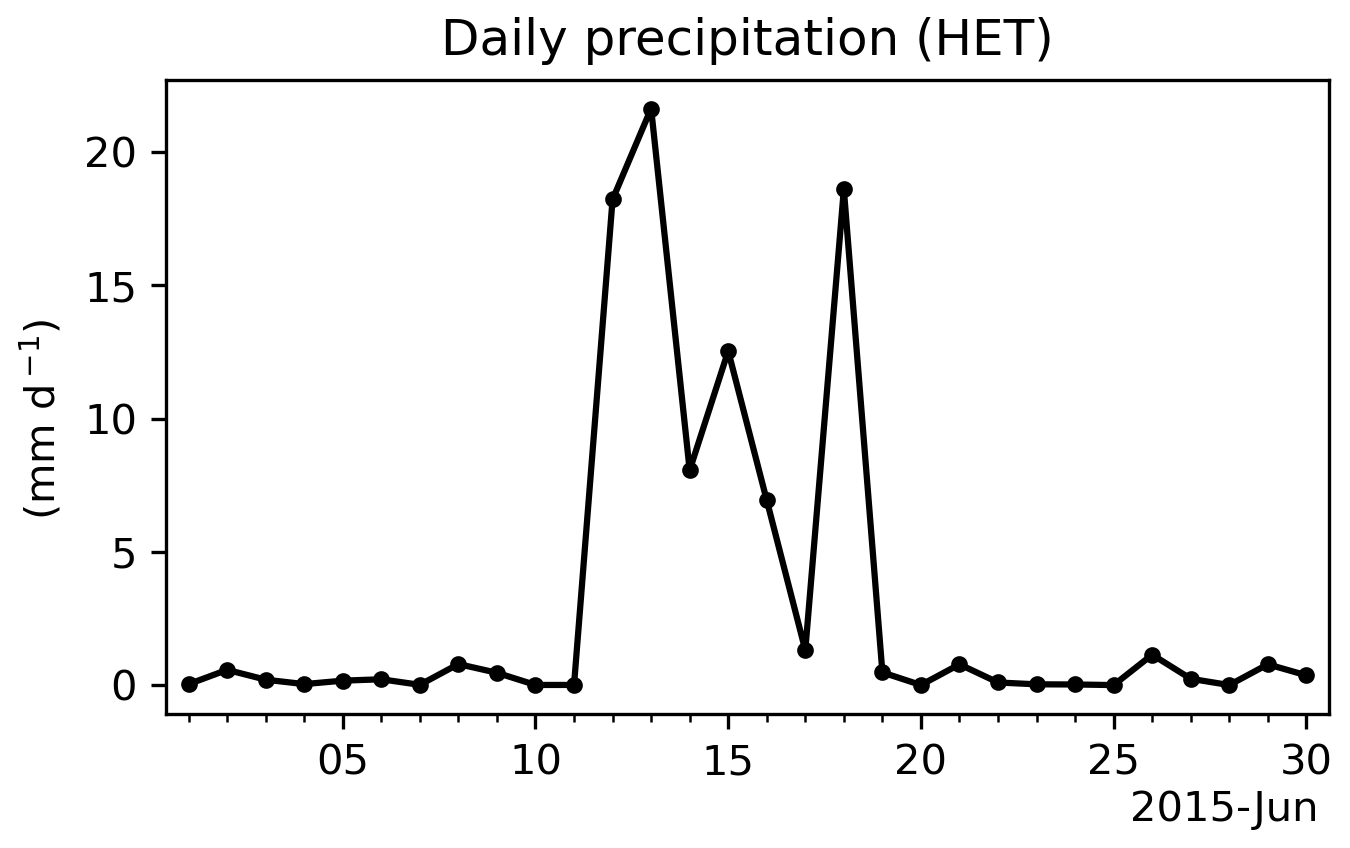
The fact that the new HET approach does not influence the precipitation characteristics in the E3SM SCM is an interesting feature. We find that it is due to the fact that the inter-patch variability, which is the dominant term in the grid-aggregated variability representing the surface heterogeneity (Eq. 8), vanishes when precipitation occurs. The sums of the area-weighted values are found to be close to zero during mid-June (see Fig. 5), coinciding with the occurrence of precipitation (Fig. 14). The exact relationship between inter-patch variances and rainfall events is found in other periods as well (not shown). This might be related to the fact that only the grid-box averaged precipitation flux is provided to the land model by the atmosphere model so that every land surface patch receives an equal amount of water from the atmosphere model, which reduces the inter-patch variability. On the other hand, the changes in cloud cover and solar radiation simulated by the atmosphere model are also uniformly applied to the patches so that the patch differences may be especially small under this energy-limited (precipitation) regime. Nonetheless, the mechanism driving this model behavior requires further investigation.

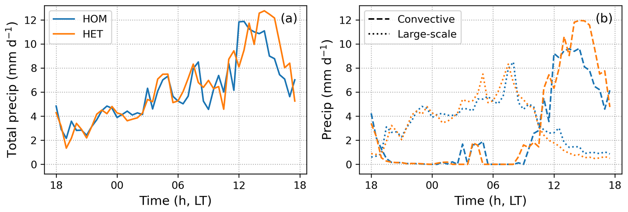
Figure 12 Diurnal cycle of (a) total precipitation and (b) convective versus large-scale precipitation from the HOM and HET SCM simulations averaged over 50 precipitating days out of the study period.

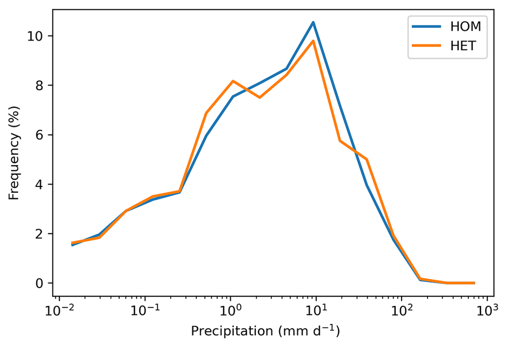
Figure 13 Frequency of occurrence of total precipitation from HOM and HET SCM simulations during the period of the precipitating days.

Figure 14 Daily precipitation simulated by HET configuration in June.

4 Conclusions

In this study, we implemented the Machulskaya and Mironov (2018) approach that aggregates the patch characteristics into equivalent grid-cell quantities to account for surface heterogeneity in land–atmosphere coupling in E3SM. This new treatment adjusts the surface variances and covariance of potential temperature and specific water content for grid cells, enabling a consideration of spatial subgrid-scale heterogeneity in the land–atmosphere coupling. The grid-cell variances and covariance were computed offline and provided to EAM as part of the lower boundary conditions. We performed E3SM SCM hindcast simulations and compared the results with simulations using the default land–atmosphere coupling that neglects the impacts of the subgrid variability of the land surface on the atmosphere. The simulation results are divided into three categories: clear-sky days, non-precipitating cloudy days and precipitating days.

Using the new patch-aggregating approach with patch states and fluxes provided by ELM, we find that the inter-patch variability in potential temperature and specific humidity is the dominant term in representing surface heterogeneity in the grid-aggregated surface boundary condition. On clear-sky days, we find that the effects of surface heterogeneity extend from the surface to the lower ABL. While accounting for the fact that surface heterogeneity increases temperature and humidity variances as expected, it reduces the temperature–humidity covariance in the afternoon since drier/wetter patches have less/more evaporation and hence higher/lower temperature.

Furthermore, we find that the increase in the surface scalar variances, as well as the decrease in the temperature–humidity covariance, can directly influence the buoyancy terms and further the turbulent fluxes of temperature and humidity in the lower ABL. We also find that the third-order moment of vertical velocity $\stackrel{\mathrm{‾}}{{w^{\prime }}^{\mathrm{3}}}$ is very sensitive to the new land–atmosphere coupling. The increase in $\stackrel{\mathrm{‾}}{{w^{\prime }}^{\mathrm{3}}}$ induced by the heterogeneous surface properties is pronounced throughout the entire ABL.

On non-precipitating cloudy days, we find that both low-level cloud fraction and liquid water content increase when surface heterogeneity is considered. These changes are accompanied by the decrease in the skewness of the subgrid vertical velocity PDF, Sk_w, indicating the change in the turbulence structure toward a more symmetric turbulent mixing in cloud layers. The changes in low-level clouds also affect the surface radiative flux as well as sensible and latent heat fluxes.

Even though the new land–atmosphere coupling introduces significant changes on clear-sky days and non-precipitating cloudy days, it does not have significant effects on precipitation. We find that the subgrid inter-patch variability vanishes when precipitation occurs. This is so that the surface moments computed using the new approach are similar to those computed by the original homogeneous treatment in land–atmosphere coupling. As a result, precipitation is not affected by this new treatment.

The patch-aggregating approach considers the subgrid variability in surface states, improving the realism of the heterogeneous land–atmosphere interactions in E3SM. This study provides an initial assessment of this treatment in a state-of-the-art ESM in an SCM configuration. This configuration allows us to improve the mechanistic understanding without being confounded by complex feedback in the atmosphere. The significant effects of this treatment on turbulence structure in the ABL and low-level clouds highlight the importance of accounting for the subgrid variability in land–atmosphere coupling. Our ongoing effort is to investigate the full climatic impacts of accounting for surface heterogeneity using global E3SM simulations. Results will be documented in a separate paper.