Comparison and evaluation of updates to WRF-Chem (v3.9) biogenic emissions using MEGAN

Biogenic volatile organic compounds (BVOCs) emitted from the natural ecosystem are highly reactive and can thus impact air quality and aerosol radiative forcing. BVOC emission models (e.g., Model of Emissions of Gases and Aerosols from Nature – MEGAN) in global and regional chemical transport models still have large uncertainties in estimating biogenic trace gases because of uncertainties in emission activity factors, specification of vegetation type, and plant emission factors. This study evaluates a set of updates made to MEGAN v2.04 in the Weather Research and Forecasting model coupled with chemistry (WRF-Chem version 3.9). Our study considers four simulations for each update made to MEGAN v2.04: (i) a control run with no changes to MEGAN, (ii) a simulation with the emission activity factors modified following MEGAN v2.10, (iii) a simulation considering the changes to the plant functional type (PFT) emission factor, and (iv) a simulation with the isoprene emission factor calculated within the MEGAN module instead of being prescribed by the input database. We evaluate two regions, Europe and the southeastern United States, by comparing WRF-Chem results to ground-based monitoring observations in Europe (i.e., AirBase database) and aircraft observations obtained during the NOMADSS field campaign. We find that the updates to MEGAN v2.04 in WRF-Chem caused overpredictions in ground-based ozone concentrations in Europe and in isoprene mixing ratios compared to aircraft observations in the southeastern US. The update in emission activity factors caused the largest biases. These results suggest that further experimental and modeling studies should be conducted to address potential shortcomings in BVOC emission models.

1 Introduction

Biogenic emissions of volatile organic compounds play a fundamental role in atmospheric chemistry, specifically in the ozone cycle and in the formation of secondary organic aerosols with implications for air quality and climate. The major biogenic volatile organic compounds (BVOCs) are isoprene and monoterpenes (e.g., α- and β-pinene) with relative contributions of 69.2 % and 10.9 %, respectively (Sindelarova et al., 2014). Emissions of BVOCs have implications for air quality by affecting the concentration of ground-level ozone (Fehsenfeld et al., 1992; Curci et al., 2010; Sartelet et al., 2012; Sindelarova et al., 2014) and for climate through tropospheric ozone radiative forcing (Brasseur et al., 1998; Gauss et al., 2006). Churkina et al. (2017) estimated that the impact of BVOC emissions on ground-level ozone production was on average 12 % in summer and up to 60 % during a heatwave event in the Berlin–Brandenburg metropolitan area, Germany. With climate change, the increase in isoprene emissions from vegetation due to higher temperatures may lead to higher tropospheric ozone concentrations (EEA, 2015). In addition to the consequences for the gas-phase chemistry, oxidative products of some BVOCs can form secondary organic aerosol (Limbeck et al., 2003; van Donkelaar et al., 2007) with significant effects on the Earth's radiation budget.

The proper quantification of BVOCs emitted into the atmosphere is a fundamental parameter in order to represent their effect reliably in global and regional chemical transport models (CTMs). Therefore, several modeling approaches have been developed for the estimation of BVOC emissions (Guenther et al., 1995; Niinemets et al., 1999; Martin et al., 2000; Arneth et al., 2007). A fundamental step towards BVOC modeling relates to the work by Guenther et al. (2006) (G06 hereafter), who developed the Model of Emissions of Gases and Aerosols from Nature version 2.0 (MEGAN v2.0) for both regional and global BVOC emission modeling. Several gaps in BVOC emission modeling were addressed in recent releases of MEGAN version 3 and MEGAN version 3.1 (Guenther et al., 2020), including BVOC emissions (i) accounting for sub-grid vegetation distribution in addition to the dominant vegetation type and (ii) induced by environmental stresses (i.e., extreme weather and air pollution events). Various global- and regional-scale chemistry transport models have adopted MEGAN as their BVOC emission model, including the Weather Research and Forecasting model coupled with chemistry (WRF-Chem – Grell et al., 2005; Fast et al., 2006). Zhao et al. (2016) used two versions (v2.04 and v2.1) of MEGAN in order to investigate the sensitivity of WRF-Chem simulated BVOC emissions with different land surface schemes: the Community Land Model version 4.0 (CLM4 – Oleson et al., 2010; Lawrence et al., 2011) and the Noah land surface model (Niu et al., 2011). The land surface schemes quantify land surface processes, their effect on near-surface meteorological conditions, and consequently the simulated BVOC emissions and concentrations. One major difference between the Noah land surface model and CLM4 is that they use different vegetation maps, and this affects BVOC emissions. Zhao et al. (2016) found that BVOC emissions modeled with MEGAN v2.04 were negligible between the two runs with different land surface schemes and the same vegetation map, whereas considering the same land surface scheme with different vegetation maps leads to large differences in simulated BVOC emissions predicted with MEGAN v2.1. Henrot et al. (2017) implemented MEGAN v2.1 in ECHAM-HAMMOZ (ECHAM6 atmospheric general circulation model; HAM aerosol model; MOZART chemistry transport model). Henrot et al. (2017) found that the emission factor and PFT distributions most strongly determine the spatial emission distribution in MEGAN, in agreement with other previous studies that used different meteorological models (Sindelarova et al., 2014; Messina et al., 2016). Jiang et al. (2019) utilized the WRF-CAMx (WRF meteorology model; CAMx regional air quality model) modeling package to investigate the effect of BVOC emissions on the surface ozone levels in Europe. They found higher (about 3 times) isoprene emissions predicted with MEGAN v2.1 compared to another BVOC emission model (i.e., Paul Scherrer Institute model – Andreani-aksoyoglu and Keller, 1995), resulting in about 10 % higher ozone mixing ratios. Therefore, Jiang et al. (2019) suggested that ozone production occurs generally in VOC-saturated rather than VOC-sensitive regimes in Europe. A few tree species dominate the total isoprene and monoterpene emissions in European forests, with three Quercus species and five types of tree species contributing to 66 % and 80 % of total isoprene and monoterpene emissions, respectively (Keenan et al., 2009). In the work by Wang et al. (2021) the impact of BVOC emissions evaluated with MEGAN version 3.1 on O₃ concentrations simulated with WRF/CAMx varied highly with the drought configurations, with the highest BVOC contribution to ozone concentrations not including drought stress. Further, because of the complex nature of representing BVOC emissions, previous studies (Messina et al., 2016; Zhang et al., 2021) recommended more measurement campaigns of BVOC emissions to validate BVOC model results.

As noted above, Zhao et al. (2016) implemented MEGAN v2.1 in WRF-Chem with the CLM4 land model; the CLM surface scheme and associated subroutines in the physics and chemistry packages have been modified to be consistent with the MEGAN v2.1 biogenic emissions. These changes became part of the community version of WRF-Chem in 2021 with the release of WRF version 4.3. In our work, which we performed before WRF version 4.3 was available, we use WRF-Chem version 3.9 to explore the effect of making changes to the existing WRF-Chem MEGAN v2.04 emissions scheme. Because we modified the MEGAN v2.04 code, our method results in having changes that can be used with the Noah land surface model. In Sect. 2, we describe the changes that were made to MEGAN v2.04.

To compare different updates to MEGAN v2.04 introduced by G12 with MEGAN v2.10 in simulating BVOC emissions, two case studies were performed in two different domains (i.e., Europe and the southeastern United States). Since ozone is known to be a result of photochemistry involving nitrogen oxides (NO_x= NO + NO₂) and volatile organic compounds (VOCs), a sensitivity study on BVOC emissions was performed for a high-ozone episode in August 2015 in Europe considering different updates to MEGAN v2.04 introduced with MEGAN v2.10. For this case study, comparisons are presented between modeled ozone concentrations and surface measurements (AirBase database – https://www.eea.europa.eu/data-and-maps/data/aqereporting-9, last access: 2 February 2018). Summer 2015 was among the six hottest and driest summers since 1950 in Europe (Ionita et al., 2017). These meteorological conditions together with four heatwave episodes led to high tropospheric ozone levels throughout Europe, with 18 of the EU-28 countries exceeding the EU ozone threshold value for the protection of human health (EEA, 2017). Lin et al. (2020) reported a link between ozone episodes in Europe and the ecosystem–atmosphere interactions during heatwaves and droughts, with lower ozone uptake by water-stressed vegetation exacerbating the peak ozone events. For the southeastern United States case study, BVOC emissions calculated with MEGAN v2.04 and MEGAN v2.10 were evaluated against aircraft measurements. Measurements of isoprene, two products of isoprene oxidation (i.e., methacrolein and methyl vinyl ketone), and ozone were taken in five of the research flights under the Southern Oxidant and Aerosol study (SOAS) in June 2013. The SOAS project is part of the Nitrogen, Oxidants, Mercury and Aerosol Distributions, Sources and Sinks (NOMADSS) project (https://www.eol.ucar.edu/field_projects/nomadss, last access: 12 September 2017) under the umbrella of the Southeast Atmosphere Study (SAS – https://data.eol.ucar.edu/project/SAS, last access: 12 September 2017), a project aimed at investigating the interactions between the atmosphere and biosphere as well as the role of BVOCs in atmospheric chemistry in the southeastern and central United States. A synthesis of relevant results achieved within SAS was presented by Carlton et al. (2018). Section 3 describes these two cases in more detail and the WRF-Chem v3.9 configurations to represent the two cases. In Sect. 4, the effects of specific updates to MEGAN v2.04 are examined and evaluated with observations from each of the case studies. A summary and conclusions are given in Sect. 5.

2 Materials and methods

MEGAN estimates the emissions considering meteorology (e.g., temperature, solar radiation, and soil moisture), leaf area index (LAI), and PFT as driving variables, with higher emissions occurring for higher values of temperature, transmission of photosynthetic photon flux density, and LAI. MEGAN v2.0 was used for analyzing the impact of biogenic emissions with potential future increases in ambient temperature on ozone levels (Im et al., 2011), aerosol levels, and chemical compositions (Im et al., 2012). Building on MEGAN v2.0 G06) and MEGAN v2.02 (Sakulyanontvittaya et al., 2008), Guenther et al. (2012) (G12 hereafter) introduced additional compounds, emission types, and controlling processes with MEGAN v2.1. In MEGAN v2.1, the emission factors are adjusted to consider that the measured net flux of BVOCs above the vegetation canopy does not involve the dry deposition flux so that the net primary emissions would be higher (e.g., up to a few percent for isoprene). To better depict the variability of isoprene emissions within a PFT category, MEGAN v2.1 allows specific PFT emission factors for each vegetation type.

2.1 Updates to MEGAN v2.04 in WRF-Chem

The Model of Emission of Gases and Aerosols from Nature (MEGAN) estimates the net emission rate of 134 chemicals species (e.g. isoprene, monoterpenes, oxygenated compounds, sesquiterpenes, and nitrogen oxide) from terrestrial ecosystems into the above-canopy atmosphere with a resolution of 1 km² (G06). MEGAN can be used in global models, such as GEOS-Chem (Goddard Earth Observing System) (Bey et al., 2001) and CAM-Chem (Community Atmosphere Model) (Tilmes et al., 2015; Lamarque et al., 2012), and regional CTMs, such as WRF-Chem (Grell et al., 2005; Fast et al., 2006).

The BVOC emission algorithm currently applied to WRF-Chem is calculated as follows:

$$\begin{array}{}\text{(1)}& \mathrm{EM}=\mathit{\epsilon }\cdot {\mathit{\gamma }}_{\mathrm{P}}\cdot {\mathit{\gamma }}_T\cdot {\mathit{\gamma }}_{\mathrm{age}}\cdot {\mathit{\gamma }}_{\mathrm{SM}}\cdot {\mathit{\gamma }}_{\mathrm{LAI}}\cdot \mathit{\rho },\end{array}$$

where EM is the BVOC emission rate (µg m⁻² h⁻¹); ε is the emission factor (µg m⁻² h⁻¹); γ_P, γ_T, γ_age, γ_SM and γ_LAI are the emission activity factors that respectively account for photosynthetic photon flux density, temperature, leaf age, soil moisture, and LAI (normalized ratio); and ρ is the loss and production within the plant canopy (normalized ratio). The emission rate (EM) is calculated for each PFT, added up to estimate the total emission at each model grid cell, and corrected considering the deviation from the standard condition (γ and ρ parameters). The factors γ and ρ are equal to unity at standard conditions (e.g., air temperature 303 K, specific humidity 14 g kg⁻¹, wind speed 3 m s⁻¹, and soil moisture 0.3 m³ m⁻³), while they are different from unity with non-standard conditions (G06).

Note that this work simply replaces equations in the MEGAN v2.04 code with the equations in MEGAN v2.10. Table 1 lists the equations from MEGAN 2.04 with what they were replaced with from the MEGAN v2.10 paper (G12). One difference between this work and that of G12 is that this paper retains four plant functional types, while G12 use 15 plant functional types. Details on the update of emission factors for this paper are given in Sect. 2.3.

Table 1 The emission activity factor equations referred to in MEGAN version 2.04 (M2.04) and the relative updates made for version 2.10 (M2.10).

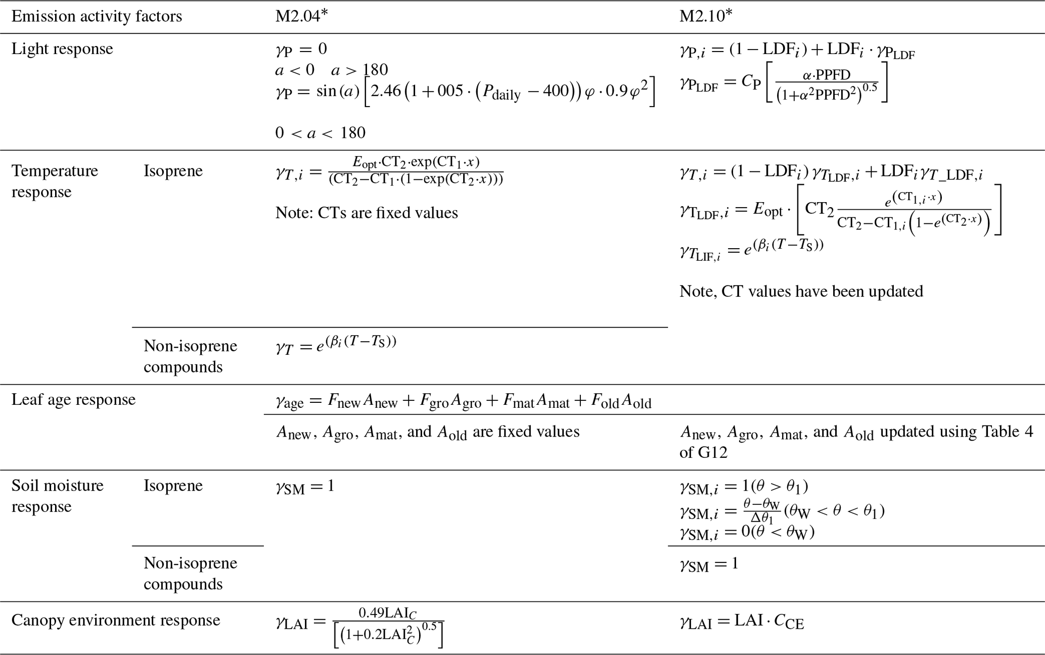
^* See text for definitions of variables.

In the present study, we made four simulations, the first three with the following configurations: (i) the control run with no changes (M2.04), (ii) the updates to the emission activity factors (i.e., gamma equations for LAI, photosynthetic photon flux density – PPFD, temperature, soil moisture, and canopy environment) following the G12 paper (MG), and (iii) the updates to the emission factor for four PFTs (MGPFT). With this third simulation we had two effects: firstly, α-pinene emissions changed from the MG simulation to the MGPFT simulation, and secondly isoprene emissions did not change from the MG to the MGPFT simulation. In the MGPFT simulation, the changes to PFT emission factor and PFT percentage in the code did not affect isoprene as its emission factor was considered directly from the pre-processor MEGAN. (iv) We forced the code to calculate the isoprene emissions as the other compounds were determined, instead of directly reading the emission factor value from the database as in the previous simulations. This resulted in isoprene emissions changing from the previous simulation (i.e., MGPFTISO different from MGPFT), while α-pinene remained the same (i.e., MGPFTISO identical to MGPFT).

2.2 Update of the emission activity factors

Emission activity factors describe variations in BVOC emissions related to physiological and phenological processes. The capability of a leaf to emit isoprene depends on a number of physical and biological factors, with incident photosynthetic photon flux density and leaf temperature as driving factors (Guenther et al., 1993). A leaf's capacity to emit isoprene is also influenced by leaf phenology, with very young leaves emitting no isoprene and mature leaves emitting isoprene maximally. Moreover, soil characteristics play a role in the plant BVOC emission ability, with droughts significantly decreasing isoprene emission (G06; Jiang et al., 2018).

The integration of MEGAN with CTM parameters (e.g., temperature, solar radiation, and soil moisture) allows an improved analysis of interactions between BVOC emissions, the surrounding environment, and the canopy itself. The standard MEGAN environment model is based on the methods described by Guenther et al. (1999), who estimated incident PPFD and temperature at five canopy depths, including a leaf isoprene-emitting model driven by humidity, solar radiation, ambient temperature, and soil moisture. Overall, the BVOC emissions are a product of both the local weather at the time of simulation (i.e., temperature, humidity, and PPFD) and long-term conditions, such as the conditions over the past month (i.e., based on seasonal conditions like soil moisture and heatwaves or drought). Therefore, the emissions are a function of both the instantaneous temperature and the temperature averaged over 1–10 d. Several algorithms have been widely used to simulate the response of isoprene emissions to changes in light, temperature, leaf age, and soil moisture (Guenther et al., 1995, 1999, 1993). However, complexity and expensive computational costs hindered their use in CTMs. To minimize computational costs, G06 developed a parameterized canopy environment emission activity (PCEEA) algorithm as an alternative to calculating all variables at each canopy. The PCEEA procedure includes algorithms for the solar radiation, temperature, and canopy environment response emission activity factors (i.e., γ_P, γ_T, and γ_LAI) in MEGAN v2.04.

2.2.1 Light response emission activity factor

One of the main advances introduced with MEGAN v2.10 is that the emission activity factors of each compound class are comprised of a light-dependent fraction (LDF) and a light-independent fraction (LIF). MEGAN v2.04 calculates the light response emission activity (γ_P) using the sine of the solar angle with no distinction between the light-dependent and light-independent fractions (Eqs. from 10 to 13 of G06) (Table 1). For each compound class, the updated emission activity factor is calculated for the PPFD variations as follows:

$$\begin{array}{}\text{(2)}& {\displaystyle }{\mathit{\gamma }}_{\mathrm{P},i}& {\displaystyle }=\left(\mathrm{1}-{\mathrm{LDF}}_i\right)+{\mathrm{LDF}}_i{\mathit{\gamma }}_{{\mathrm{P}}_{\mathrm{LDF}}},\text{(3)}& {\displaystyle }{\mathit{\gamma }}_{{\mathrm{P}}_{\mathrm{LDF}}}& {\displaystyle }=C_{\mathrm{P}}\left[{\displaystyle \frac{\mathit{\alpha }\cdot \mathrm{PPFD}}{{\left(\mathrm{1}+{\mathit{\alpha }}^{\mathrm{2}}\cdot {\mathrm{PPFD}}^{\mathrm{2}}\right)}^{\mathrm{0.5}}}}\right],\text{(4)}& {\displaystyle }{C}_{\mathrm{P}}& {\displaystyle }=\mathrm{0.0468}\cdot e^{(\mathrm{0.0005}\times [P_{\mathrm{24}}-P_{\mathrm{s}}\left]\right)}\cdot {\left[P_{\mathrm{240}}\right]}^{\mathrm{0.6}},\text{(5)}& {\displaystyle }\mathit{\alpha }& {\displaystyle }=\mathrm{0.004}-\mathrm{0.0005}\ln \left(P_{\mathrm{240}}\right),\end{array}$$

where the PPFD is the instantaneous photosynthetic photon flux density (µmol m⁻² s⁻¹), P_s represents the standard conditions for PPFD averaged over the past day (200µmol m⁻² s⁻¹ for sun leaves and 50 µmol m⁻² s⁻¹ for shade leaves), P₂₄ is the average PPFD of the past 24 h, and P₂₄₀ is the average PPFD of the past 10 d (Table 1). Version 2.10 calculates the γ_P with the photosynthetic photon flux density using the internal variable “swdown”: the downward solar radiation (W m⁻²). P₂₄ and P₂₄₀ are the average PPFD of the past day and the past 10 d. Nevertheless, they are both equal to the “mswdown” variable: the downward solar radiation (W m⁻²) of the previous month (G12).

2.2.2 Temperature response emission activity factor

In MEGAN v2.04, the temperature activity factor (γ_T) calculates the response emission activity for isoprene according to Eq. (5) and Eqs. (8) and (15) by G06; all the other non-isoprenoid compounds are described according to the monoterpene exponential temperature response function by Guenther et al. (1993).

The updated temperature activity factor (MEGAN v2.10) leads to two different changes: (i) the introduction of LDF and LIF (i.e., as the previous emission factor) and (ii) the dependency on the specific compound classes instead of the isoprene and non-isoprene species. The updated version of the LDF of the temperature activity factor (γ_T) is calculated as follows:

$$\begin{array}{}\text{(6)}& {\displaystyle }{\mathit{\gamma }}_{T,i}& {\displaystyle }=\left(\mathrm{1}-{\mathrm{LDF}}_i\right){\mathit{\gamma }}_{T_{\mathrm{LDF}},i}+{\mathrm{LDF}}_i\cdot {\mathit{\gamma }}_{T\mathit{\_}\mathrm{LDF},i},\text{(7)}& {\displaystyle }{\mathit{\gamma }}_{T_{\mathrm{LDF}},i}& {\displaystyle }=E_{\mathrm{opt}}\cdot \left[{\mathrm{CT}}_{\mathrm{2}}{\displaystyle \frac{e^{\left({\mathrm{CT}}_{\mathrm{1},i}x\right)}}{{\mathrm{CT}}_{\mathrm{2}}-{\mathrm{CT}}_{\mathrm{1},i}\left(\mathrm{1}-e^{\left({\mathrm{CT}}_{\mathrm{2}}\cdot x\right)}\right)}}\right],\text{(8)}& {\displaystyle }x& {\displaystyle }={\displaystyle \frac{\left[\left(\frac{\mathrm{1}}{T_{\mathrm{opt}}}\right)-\left(\frac{\mathrm{1}}{T}\right)\right]}{\mathrm{0.00831}}},\text{(9)}& {\displaystyle }{E}_{\mathrm{opt}}& {\displaystyle }=C_{\mathrm{eo},i}\cdot e^{(\mathrm{0.05}\cdot \left(T_{\mathrm{24}}-T_{\mathrm{S}}\right))}\cdot e^{\left(\mathrm{0.05}\left(T_{\mathrm{240}}-T_{\mathrm{S}}\right)\right)},\text{(10)}& {\displaystyle }{T}_{\mathrm{opt}}& {\displaystyle }=\mathrm{313}+\left(\mathrm{0.6}\cdot \left(T_{\mathrm{240}}-\mathrm{297}\right)\right),\end{array}$$

where E_opt is the maximum normalized emission capacity (mol km⁻² h⁻¹); T_opt is the temperature at which E_opt occurs (K); T is the leaf temperature (K) assumed to be the air temperature at 2 m (T2) calculated by WRF at each grid point; CT_1−i, CT₂, and C_eo−i are emission-class-dependent empirical coefficients; T_S represents the standard conditions for leaf temperature (297 K); T₂₄ is the average leaf temperature of the past 24 h (K); and T₂₄₀ is the average leaf temperature of the past 240 h (K).

The response of LIF is determined according to the monoterpene exponential temperature response function by Guenther et al. (1993):

$$\begin{array}{}\text{(11)}& {\mathit{\gamma }}_{T_{\mathrm{LIF},i}}=e^{\left({\mathit{\beta }}_i\left(T-T_{\mathrm{S}}\right)\right)},\end{array}$$

where β_i is an empirically determined coefficient depending on the emission compound class (G12).

Additional changes made to this part of the code concern the update of the CT₁, CT₂, and C_eo parameters. In G06 their values are respectively set to 80, 200, and 1.75, whereas CT_1,i and C_eo,i depend on the compound classes, and CT₂ still has a fixed value (i.e., 230) in the updated version (Table 1). A more accurate BVOC evaluation with each compound class having the appropriate value may result from (i) the temperature activity factor defined as the weighted average of a light-dependent and light-independent fraction (${\mathit{\gamma }}_{T_{\mathrm{LDF},i}}$ and ${\mathit{\gamma }}_{T_{\mathrm{LIF},i}}$) (ii) and the update of the model parameters (CT₁, CT₂, and C_eo) for each compound class. Note that the values of T₂₄ and T₂₄₀ are estimated as equal to the variable monthly surface air temperature (MTSA) with MEGAN v2.10. Therefore, it is assumed that the average temperature of the past 24 h and the past 10 d is the same as the average temperature of the past month ($T_{\mathrm{24}}=T_{\mathrm{240}}=$ MTSA).

2.2.3 Leaf age response emission activity factor

The canopy isoprene-emitting capability is also influenced by the leaf age. An increase in foliage is assumed to imply a growing production of isoprene (young leaves), whereas decreasing foliage is associated with less production of isoprene (old leaves). Guenther et al. (1999) developed an algorithm with a time step of 1 month to simulate the emissions change for young, mature, and old leaves. The algorithm adapted to MEGAN v2.04 assumes a constant value (γ_age=1) for evergreen canopies, while deciduous canopies are divided into four fractions: new foliage (F_new), growing foliage (F_gro), mature foliage (F_mat), and old foliage (F_old). The leaf age factor is computed as

$$\begin{array}{}\text{(12)}& {\mathit{\gamma }}_{\mathrm{age}}=F_{\mathrm{new}}{A}_{\mathrm{new}}+F_{\mathrm{gro}}{A}_{\mathrm{gro}}+F_{\mathrm{mat}}{A}_{\mathrm{mat}}+F_{\mathrm{old}}{A}_{\mathrm{old}},\end{array}$$

where A_new, A_gro, A_mat, and A_old are the relative emission rates assigned to each canopy fraction depending on PFT category. The canopy is divided into leaf age fractions based on the change in LAI between the current time step (current month = LAI_c) and the previous time step (previous month = LAI_p). The difference between the two LAI values describes the leaf area index age. No difference in LAI (i.e., LAI_p= LAI_c) indicates a canopy mostly formed by mature foliage. A canopy is formed by old foliage when the LAI value of the previous month is greater than the one in the current month (LAI_p> LAI_c), whereas LAI_p< LAI_c for a canopy primarily formed by new foliage (G06).

MEGAN v2.10 estimates the leaf age emission activity factor (γ_age) in Eq. (12) based on the same calculations described by Eq. (16) in G06. The two versions of MEGAN do not differ for the canopy subdivision into four fractions (i.e., new foliage – F_new, growing foliage – F_gro, mature foliage – F_mat, and old foliage – F_old) and the related computation. The only update of equation parameters is the relative emission rates assigned to each compound class (A_new, A_gro, A_mat, and A_old) reported in Table 4 of G12 (Table 1).

2.2.4 Soil moisture response emission activity factor

Different studies have shown that isoprene emission decreases when soil moisture drops below a threshold and eventually becomes insignificant when plants are exposed to extended drought (Jiang et al., 2018; Pegoraro et al., 2004). In the WRF-Chem version of MEGAN v2.04, the soil moisture activity factor (γ_SM) is set to 1.0 for both isoprene and non-isoprene compound classes. Therefore, the soil moisture dependence is not involved in the BVOC emissions algorithm. In the present study, (in MEGAN v2.10 code applied to WRF-Chem), isoprene emissions were evaluated according to Eqs. (20a), (20b), and (20c) described by G06 as follows.

$$\begin{array}{}\text{(13)}& {\displaystyle }{\mathit{\gamma }}_{\mathrm{SM},\mathrm{isoprene}}& {\displaystyle }=\mathrm{1}(\mathit{\theta }>{\mathit{\theta }}_{\mathrm{1}})\text{(14)}& {\displaystyle }{\mathit{\gamma }}_{\mathrm{SM},\mathrm{isoprene}}& {\displaystyle }={\displaystyle \frac{\mathit{\theta }-{\mathit{\theta }}_{\mathrm{W}}}{\mathrm{\Delta }{\mathit{\theta }}_{\mathrm{1}}}}({\mathit{\theta }}_{\mathrm{W}}<\mathit{\theta }<{\mathit{\theta }}_{\mathrm{1}})\text{(15)}& {\displaystyle }{\mathit{\gamma }}_{\mathrm{SM},\mathrm{isoprene}}& {\displaystyle }=\mathrm{0}(\mathit{\theta }<{\mathit{\theta }}_{\mathrm{W}})\text{(16)}& {\displaystyle }{\mathit{\gamma }}_{\mathrm{1}}& {\displaystyle }={\mathit{\gamma }}_{\mathrm{W}}+{\mathit{\gamma }}_{\mathrm{1}}\end{array}$$

Here, θ is soil moisture (m³ m⁻³), θ_W is the soil moisture threshold below which plants cannot extract water from soil (wilting point, m³ m⁻³), and Δθ₁ (=0.06) is an empirical parameter from Pegoraro et al. (2004). MEGAN uses a wilting point database that assigns different θ_w values for each soil type based on Table 2 of Chen and Dudhia (2001) (Table S1 of the Supplement). Since for G12 the non-isoprenoid soil moisture dependence is not involved in the BVOC emissions algorithm, in the present study, the γ_SM for non-isoprenoid compounds is still set to 1.0.

2.2.5 Canopy environment response emission activity factor

The emission response to leaf area index (γ_LAI) in MEGAN v2.04 calculates the response emission activity factor with Eq. (15) of G06. In MEGAN v2.10 the canopy environment coefficient has been simplified as follows:

$$\begin{array}{}\text{(17)}& {\mathit{\gamma }}_{\mathrm{LAI}}=\mathrm{LAI}\cdot C_{\mathrm{CE}},\end{array}$$

where LAI (m² m⁻²) is the leaf area index referring to the month of the simulation, and C_CE is a value dependent on the canopy environment model being used. The WRF-AQ (Weather Research Forecast – Air Quality) canopy environment model uses a value of 0.57 (G12).

2.3 Updates of PFTs and isoprene emission factors

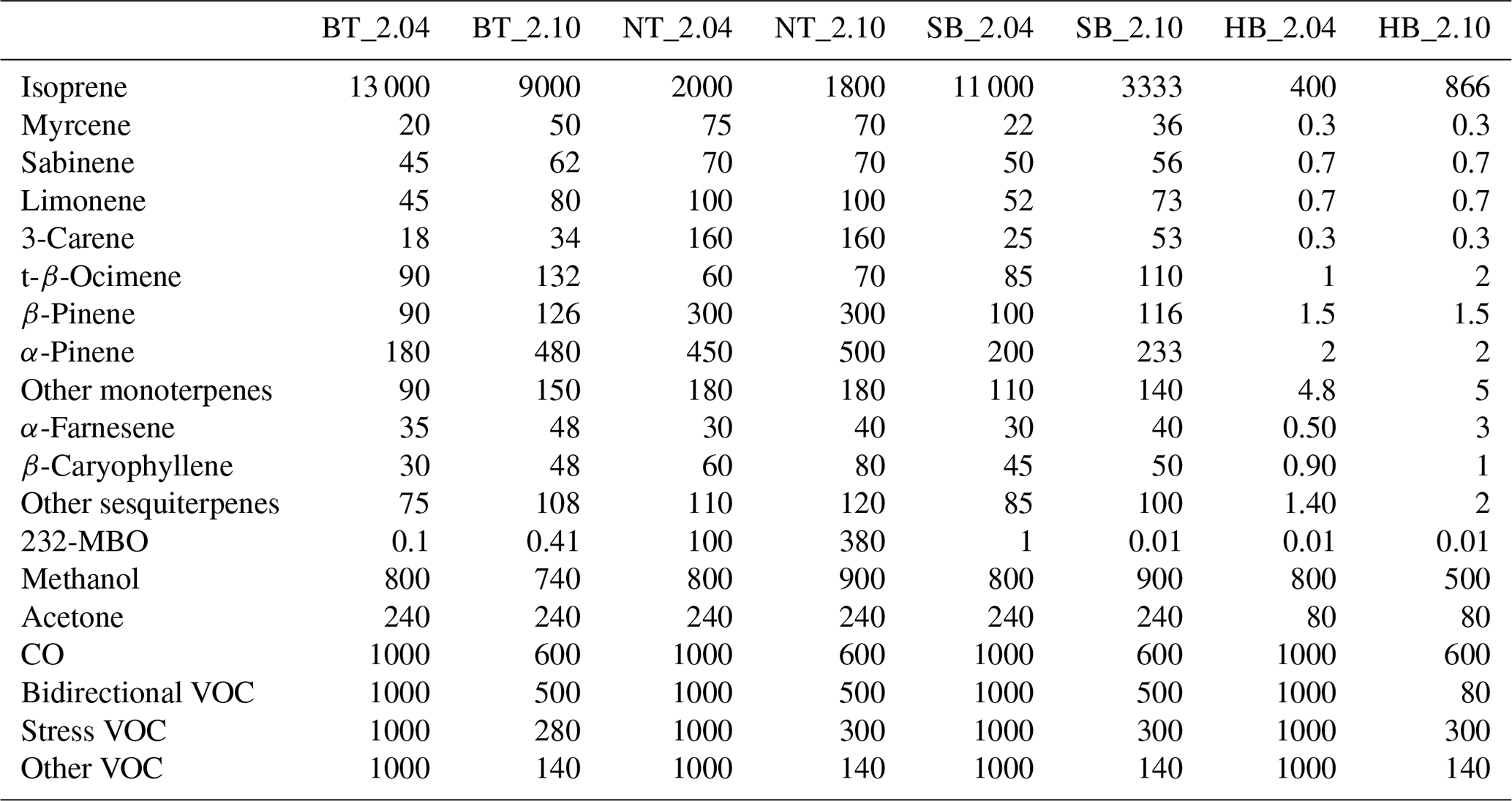
An important difference between MEGAN v2.04 and MEGAN v2.10 is the number of PFTs described and the associated isoprene emission factors. Only four PFTs are used in MEGAN v2.04, including needleleaf trees, broadleaf trees, broadleaf shrubs, and grass and other. In contrast, MEGAN v2.10 includes 15 PFTs (needleleaf evergreen temperate trees, needleleaf evergreen boreal trees, needleleaf deciduous boreal trees, broadleaf evergreen tropical trees, broadleaf evergreen temperate trees, broadleaf deciduous tropical trees, broadleaf deciduous temperate trees, broadleaf deciduous boreal trees, broadleaf evergreen temperate shrubs, broadleaf deciduous temperate shrubs, broadleaf deciduous boreal shrubs, Arctic C₃ grass, cool C₃ grass, warm C₄ grass, and crops). In order to explore the effect of the updated emission factors without revising the pre-processing code, we opted to apply a typical emission factor from G12 (Table 2) to the four PFTs currently in WRF-Chem. Table 2 shows the updated emission factors for the four PFTs and their previous value from MEGAN v2.04. The new isoprene emission factor decreased for all PFTs except for herbaceous species (HB – grass and other); at the bottom of Table 2 it is noticeable that carbon monoxide as well as the bidirectional, stress, and other VOCs decreased with new values independently of the PFT considered. For all the other compound classes, the new emission factors are larger than the previous emission factors.

Table 2 Biogenic emission classes and emission factors (new and old) (µg m⁻² h⁻¹) for each plant functional type updated to MEGAN v2.10 and applied to WRF-Chem (G12).

The PFT emission factor update does not change the isoprene emission, as its emission factors in MEGAN v2.04 implemented in WRF-Chem are estimated directly from the input database. Thus, a sensitivity simulation was performed with the isoprene emission factor evaluated according to the MEGAN emission algorithm Eq. (1) instead of the input database as outlined in Sect. 3.

3 Case study descriptions and model configuration

3.1 European case

3.1.1 Characterization of case from observations

Summer 2015 was among the six hottest and driest summers since 1950 in Europe (Ionita et al., 2017). In this year, high tropospheric ozone episodes were experienced throughout Europe, with 18 of the EU-28 countries as well as 41 % of monitoring stations reporting an ozone maximum daily 8 h mean above 120 µg m⁻³ (60.4 ppb; the current target value for ozone in Directive 2008/50/EC) on more than 25 d (EEA, 2017). Therefore, a 6 d high-ozone period (10–16 August 2015) was selected to evaluate the impact of the changes in the MEGAN v2.04 scheme on isoprene emissions and ozone mixing ratios.

The high ozone levels were confirmed by examining the summertime (May–September) hourly average ozone concentrations measured at the air quality monitoring stations in the Marche region (Italy) (Fig. 1a and b) over a period of 3 years (from 2013 to 2015). The analysis results indicate that an extraordinary ozone peak event occurred in the time period 10–16 August 2015.

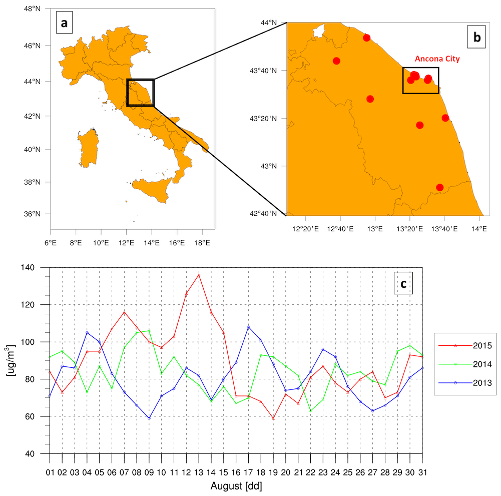
Figure 1 (a–b) Marche region (Italy) air quality monitoring stations analyzed in the 3-year study. (c) The ozone maximum daily 8 h mean (µg m⁻³) averaged over all stations (b) in the month of August 2013, 2014, and 2015 (http://85.47.105.98:16382, last access: 1 July 2021 – ARPAM).

3.1.2 Model configuration

On 13 August, all the air quality stations (i.e., Marche region air quality stations) reported the highest ozone daily 8 h mean concentration value of the whole year (Fig. 1c). To represent the evolution of the ozone peak event the simulations lasted 6 d, from 10 August (00:00 UTC) to 16 August (00:00 UTC), with 2 d of spin-up for the model. A spin-up time of 48 h is used for the chemistry to be consistent with the ambient conditions following past studies (Yerramilli et al., 2012; Zhang et al., 2009). The initial domain configuration used a nested domain over Italy with a 4×4 km grid, but instead of focusing over the Marche region of Italy, we analyze the larger domain over Europe to explore the capabilities of the updated MEGAN algorithm for different vegetation types and chemistry regimes.

The WRF-Chem model (simulation domain shown in Fig. 2) used initial and boundary conditions from the FNL (Final) Operational Global Analysis data (Ncep, 2000). These data are available every 6 h on a 1^∘ × 1^∘ spatial grid. As summarized in Table 3, the following physical schemes were used. The Morrison double-moment scheme was selected for the treatment of the microphysics processes (Morrison et al., 2009). The Rapid Radiative Transfer Model (RRTMG) for both shortwave and longwave radiation is used; this allows activating the aerosol direct radiative effect (Iacono et al., 2008) to represent scattering and absorption in the atmosphere. The Mellor–Yamada–Janjic (MYJ) parameterization was considered to describe the planetary boundary layer (Janjiæ, 1994). The unified Noah land surface model was chosen to represent the land surface interaction (Chen et al., 1996). It includes soil temperature and moisture in four layers, fractional snow cover, and frozen soil physics. The Grell–Freitas scheme was considered for the cumulus parameterization scheme: it tries to smooth the transition to cloud-resolving scales (Grell and Freitas, 2014).

Table 3 Namelist settings of the physical parameterizations used in the WRF-Chem setup simulations.

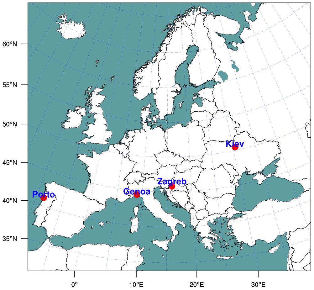
Figure 2 The numerical domain of the WRF-Chem simulations with 380 × 360 grid points and 12 km grid cells as well as the location of the four cities in Europe selected for analyzing the simulated isoprene and α-pinene emissions, namely Porto (Portugal), Genoa, (Italy), Zagreb, (Croatia), and Kyiv, (Ukraine), spanning the range 41.15–51.45^∘ N and 8.63^∘ W–30.50^∘ E.

To investigate the role of isoprene in the high-ozone event recorded in Europe, the selected chemical package was the chemical option with the Model for Ozone and Related chemical Tracers (MOZART) version 4 (Emmons et al., 2010) for the trace gases and the Model for Simulating Aerosol Interactions and Chemistry (MOSAIC) (Zaveri et al., 2008) for the aerosol-phase species. The CAM-chem (Tilmes et al., 2015; Lamarque et al., 2012) global model results are used for the chemical initial and boundary conditions for both the gas and aerosol components. The Emission Database for Global Atmospheric Research–Hemispheric Transport of Air Pollution (EDGAR-HTAP) emission inventory for Europe provided the anthropogenic emissions (Janssens-Maenhout et al., 2011). The open biomass burning emissions were from the Fire Inventory from the NCAR FINN model (Wiedinmyer et al., 2011) and the biogenic emissions from the MEGAN database (G06, G12).

Table 4 lists the four simulations conducted to study the MEGAN updates described above. The control run (M2.04) uses the MEGAN v2.04 database without any changes. The second simulation (MG) includes only the changes to the activity factors (γ). The third simulation (MGPFT) adds to the changes in the activity factors the variation of the PFT emission factors (listed in Table 2). The fourth simulation (M2.10) is the same as the MGPFT run, except the isoprene emission factor is calculated with Eq. (1) instead of being prescribed by the input data.

Table 4 Simulations performed in this study.

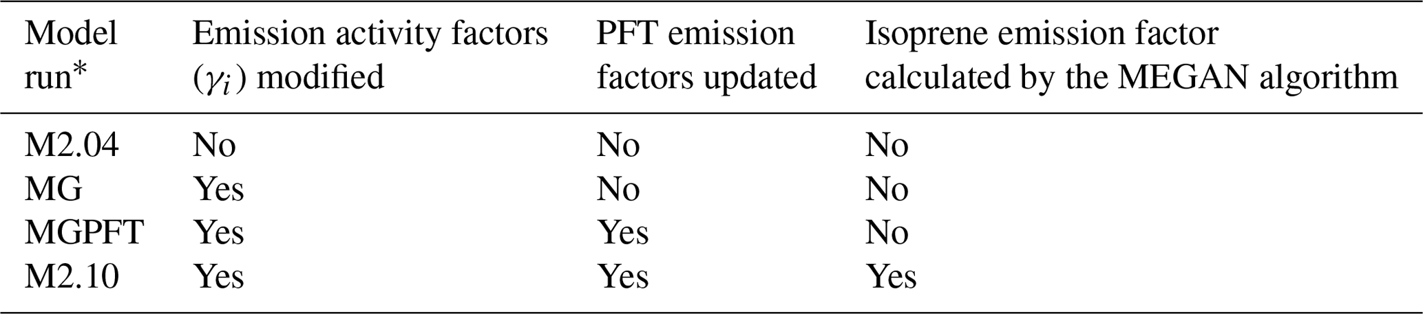
^∗ M2.04 indicates MEGAN v2.04, MG indicates only activity factors updated, MGPFT indicates activity factors and PFT emission factors updated, and M2.10 indicates MGPFT plus including the update to the isoprene emission factor.

3.2 Southeastern US Case

3.2.1 Characterization of case from observations

The NOMADSS project, which SOAS was part of, took place over the southeastern United States from 1 June to 15 July 2013. The NSF/NCAR C-130 flight tracks covered much of the eastern United States. The NOMADSS field campaign includes 19 flights from 3 June to 14 July 2013. For these flights, the aircraft sampled air in isoprene-rich emission regions (Fig. 3). Specifically, the flight tracks had high isoprene mixing ratios when the aircraft was in the boundary layer. Low isoprene mixing ratios occurred when the aircraft was above the boundary layer. For example, this trend can be observed in the time series of flight altitude (Fig. 17a) and measured isoprene concentration (Fig. 17c, black markers) for the second NOMADSS flight (rf02).

Figure 3 The x values (i.e., colored dots) denote the isoprene mixing ratios (pptv) along the aircraft flight tracks plotted over the different maps of isoprene emission factors (mol km⁻² h⁻¹) from the M2.04 simulation. Results are for each research flight day at 15:00 local time (20:00 UTC), namely (a) rf01 on 3 June 2013, (b) rf02 on 5 June 2013, (c) rf03 on 8 June 2013, (d) rf04 on 12 June 2013, and (e) rf05 on 14 June 2013.

3.2.2 Model configuration

Figure 4 shows the model domains. The coarse domain has 442 × 265 grid points with 12 km grid cells centered at 40^∘ N, 97^∘ W, covering the United States of America (USA) (CONUS domain – SW corner 22.83^∘ N, 120.49^∘ W; NW corner 52.46^∘ N, 136.45^∘ W; NE corner 45.98^∘ N, 60.82^∘ E; SE corner 20.08^∘ N, 81.24^∘ W). The nested domain is centered over the southeastern area of the USA with 301 × 301 grid points and 4 km grid cells including the selected NOMADSS flight tracks (rf01–rf05) inside the simulation domain. Both domains consider 40 vertical levels up to 50 hPa. The simulations lasted 14 d from 1 June (00:00 UTC) to 15 June (00:00 UTC) 2013. The simulations started 2 d before the first flight (rf01 – 3 June) so as to guarantee a spin-up for the model (Yerramilli et al., 2012; Zhang et al., 2009). To compare directly with the aircraft measurements, the “tracking” option was selected in WRF-Chem. This option outputs the vertical profiles of prescribed meteorological and chemical species at a set of prescribed times and horizontal coordinates taken from the location and time of the aircraft.

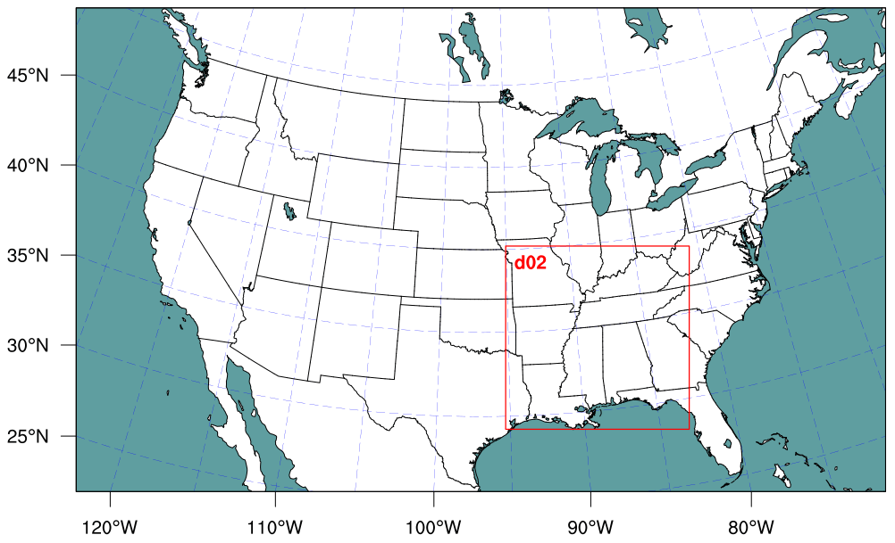
Figure 4 The numerical domains of the NOMADSS simulations: the coarse domain has 442 × 265 grid points with 12 km grid cells, and the nested domain, with 4 km grid cells, has 301 × 301 grid points.

Meteorological boundary and initial conditions were extracted from NCEP North American Regional Reanalysis (NARR – ds608.0). The NARR project is an addition to the NCEP global reanalysis, which is run only over the North American region with the 32 km grid spacing of the NCEP Eta model (NCAR, 2005). The configuration of the physical and chemical–aerosol schemes used for this part of the study is the same as that described in the previous section and reported in Table 3. Two simulations were performed to evaluate MEGAN updates with the measurements sampled by the NCAR C-130. The two simulations were M2.04 with the original MEGAN v2.04 database and M2.10 with all the code updates previously described in Sects. 2.2 and 3.1.

4 Results

4.1 European case study

In this section, we begin by describing and evaluating the synoptic meteorological conditions for 10–15 August 2015, as well as evaluating WRF-Chem temperature predictions with ground-based measurements because isoprene emissions depend strongly on temperature. Then we show how isoprene and α-pinene emissions differ among the four simulations (M2.04, MG, MGPFT, and M2.10). Lastly, since BVOC observations are not available, trace gas (NO_x, CO, and O₃) concentrations are compared between the different simulation concentration outputs with ground-based observations. The evaluation is conducted with a statistical analysis based on the calculation of mean bias, correlation coefficient, and normalized root mean square error, as well as an assessment of the spatial distribution of the NO_x, CO, and O₃ concentrations.

4.1.1 Synoptic conditions

We begin with evaluating the synoptic conditions predicted by the WRF-Chem simulations. The 6 d average geopotential height map at 850 hPa (Fig. 5a) shows the presence of an intense geopotential height maximum (1520–1580 m) affecting the central part of the Mediterranean basin in steady state for the duration of the period analyzed. The ridge separates a geopotential height minimum (1300–1340 m) over northwestern Europe from a weak depression (1460–1500 m) over Turkey. As a consequence, central and southern Europe are affected by northeasterly currents from northern Europe, allowing the weak depression to cross Italy toward the southeast portion of the domain. The WRF-Chem (Fig. 5b) simulations are consistent with the evolution represented in the reanalysis, although with some slight differences. In particular, the low pressure is more intense in the WRF-Chem runs, whereas the high pressure across Italy is more intense in the NCAR/NCEP reanalysis. Comparison between simulated (Fig. 5a) and observed (Fig. 5b) 6 d average temperature shows that the values and the spatial distribution of temperature are well depicted by the WRF-Chem model. The lowest temperatures (i.e., 5–10 ^∘C) are in northwestern Europe (i.e., Iceland). Temperatures increase in the northeasterly direction with values in the range of 10–15 ^∘C in most parts of England and the Scandinavian Peninsula. Along central and western Europe, the temperature increases up to 15–25 ^∘C (e.g., Portugal, Spain, French, Germany). Southeastern Europe (e.g., Italy, Croatia, Albania, Greece, and Turkey) has the highest temperatures up to about 30–35 ^∘C.

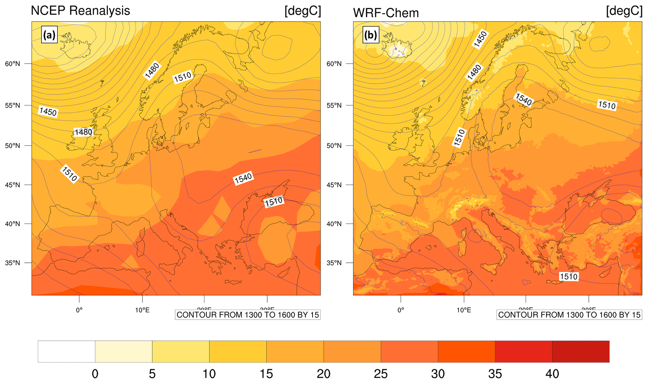
Figure 5 Comparison between the 6 d (10–15 August 2015) average geopotential height (m) at 850 hPa and mean temperature at 995 hPa, obtained with (a) NCAR/NCEP reanalysis and (b) the WRF-Chem model.

Examination of the downward shortwave radiation flux and total precipitation for the four simulations showed that these parameters do not change with the variation of the BVOC emissions (Figs. S1 and S2 in the Supplement). The ozone feedbacks do not influence the solar radiation as the ozone considered from the radiation scheme (i.e., RRTMG from Iacono et al., 2008) is a default value, and not the value calculated in the code algorithms. Even the total precipitation does not change between simulations as we did not include aerosol–cloud interactions in the simulations.

4.1.2 Examination of the MEGAN emission algorithm updates

The map of PFT percentage coverage reveals higher coverage of needleleaf trees compared to broadleaf, as well as shrub and bush in northeastern Europe with values 30 %–70 %, with a comparable trend in the north of Spain (i.e., the Cantabrian Mountains), Italy (i.e., Alps), Germany, and most parts of the Balkan Peninsula (i.e., Carpathian Mountains) (Fig. 6a–d). The broadleaf coverage has a geographical distribution similar to the needleleaf trees, but with lower values (from 10 % to 40 %). The shrub and bush PFTs are predominant in Norway, north of Russia, the southeastern part of Spain, and Turkey. Herbs cover the greatest portion of central Europe with a value 70 %–100 %, since there is a substantial number of plants that fall within this plant functional type (grass and other – PFTP_HB). The isoprene-emitting genera in this category include: Phragmites (a reed), Carex (a sedge), Stipa (a grass), and Sphagnum (a moss) (G06).

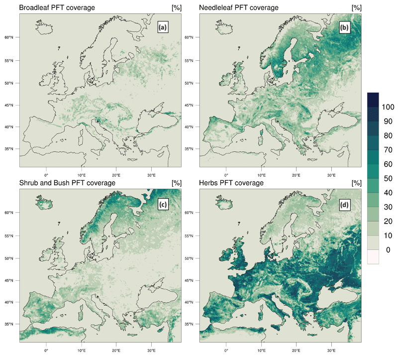
Figure 6 Percentage coverage (%) of plant functional type (PFT) classification included in the MEGAN database, computed in August 2015. From the upper left map: (a) coverage of broadleaf trees (PFTP_HB), (b) needleleaf trees (PFTP_NB), broadleaf shrubs (PFTP_SB), and (d) grass and other (PFTP_HB).

Four European cities, Porto (Portugal), Genoa (Italy), Zagreb (Croatia), and Kyiv (Ukraine), shown in Fig. 2, were selected for analyzing the time series of isoprene and α-pinene emissions. These four cities represent warmer to cooler conditions experienced over Europe and are located in areas characterized by different PFTs (Fig. 6). Figure 7a–d show the time series of isoprene emissions in the four selected cities from 10 to 16 August 2015. The isoprene diurnal cycle responds to the daily fluctuations in solar radiation. The updates applied to MEGAN v2.04 in WRF-Chem resulted in increased isoprene emissions of up to 3 times for each city analyzed. Modifying the gamma factors (MG simulation) produced the greatest increase in emissions, while modifying the PFT emission factors with isoprene emission factors obtained from the input database (MGPFT) produced the same emission magnitude as the MG simulation. Applying calculated isoprene emission factors (M2.10) gave lower isoprene emissions than MG and MGPFT, but still higher emissions than M2.04. The magnitude of the isoprene emissions varied between cities, with simulated isoprene emissions ranked as follows: Zagreb > Porto > Genoa > Kyiv. Differences in the isoprene emission magnitudes are caused by the plant functional types in each city and their respective emission factors. For example, Zagreb has about 30 %, 40 %, 20 %, and 70 % for BT, NT, SB, and HB vegetation, respectively, while Kyiv has about 10 %, 30 %, 20 %, and 90 % for BT, NT, SB, and HB vegetation, respectively (Fig. 8). Temperature and cloudiness can play a role in isoprene emission magnitude too. Figure 5 shows the temperature across Europe. Porto has the temperature in the range of 20–25 ^∘C, Zagreb 25–30 ^∘C, Genoa 20–25 ^∘C, and Kyiv 15–20 ^∘C. Also, Porto, Genoa, and possibly Kyiv look like they may have experienced cloudiness based on the shape of the diurnal profile. On clear-sky days, the isoprene emission diurnal profile is smooth with a peak at midday. Clouds that form during the day can attenuate the solar radiation, affecting the gamma-light parameter in the MEGAN calculation. In Fig. 7, the more jagged diurnal profiles of isoprene emissions are likely due to cloudiness at different times of day.

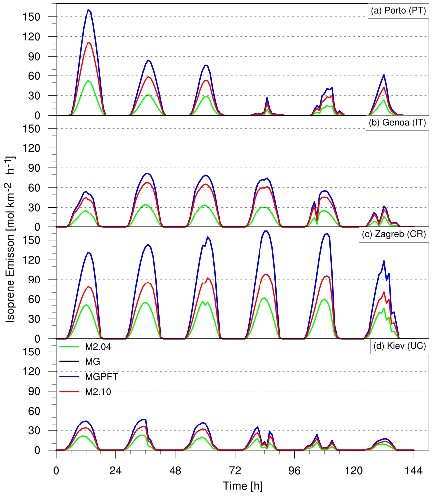
Figure 7 Time series of isoprene emissions (mol km⁻² h⁻¹) for different MEGAN algorithm configurations evaluated in four cities in Europe: (a) Porto, Portugal; (b) Genoa, Italy; (c) Zagreb, Croatia; (d) Kyiv, Ukraine. The time period considered is from 10 August 2015 at 00:00 UTC to 16 August 2015 at 00:00 UTC. The green lines represent the control simulation (M2.04), the black lines indicate the activity factor (γ) updates (MG), the blue lines are representative of the PFT emission factor updates (MGPFT), and the red lines show the isoprene emission factor as the emission factor of all the other compound classes (M2.10).

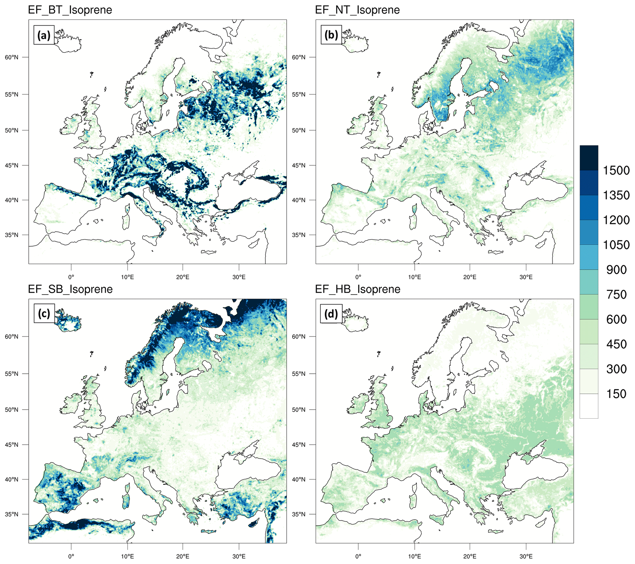
Figure 8 PFT-weighted emission factor (PFT emission factor and PFT percentage) (µg km⁻² h⁻¹) of isoprene, computed for the month of August 2015 in Europe. The emission factor values used are from Table 2 (2.10 column). From the upper left map: (a) PFT-weighted emission factor of broadleaf trees (PFTP_BT), (b) needleleaf trees (PFTP_NB), broadleaf shrubs (PFTP_SB), and (d) grass and other (PFTP_HB).

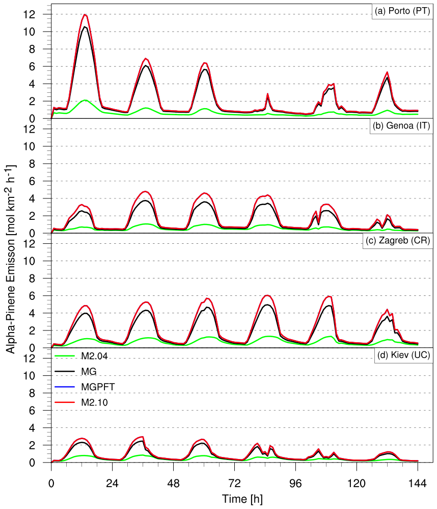
Figure 9 Time series of α-pinene emissions (mol km⁻² h⁻¹) for different MEGAN algorithm configurations evaluated in four cities in Europe: (a) Porto, Portugal; (b) Genoa, Italy; (c) Zagreb, Croatia; (d) Kyiv, Ukraine. The time period considered is from 10 August 2015 at 00:00 UTC to 16 August 2015 at 00:00 UTC. The green lines represent the control simulation (M2.04), the black lines indicate the activity factor (γ_i) updates (MG), the blue lines are representative of the PFT emission factor updates (MGPFT), and the red lines show the isoprene emission factor as the emission factor of all the other compound classes (M2.10).

Figure 9a–d show the time series of α-pinene emissions for the selected cities from 10 to 16 August 2015. Among the monoterpene compounds, α-pinene is the highest contributor to the global annual BVOC emissions (Henrot et al., 2017). In each city, α-pinene emissions show daily patterns with peaks in the daytime and plateaus in the nighttime, as with the isoprene emissions but an order of magnitude lower. In each of the cities analyzed, the simulated α-pinene emissions ranked as follows: MGPFT ≡ M2.10 > MG > M2.04. The α-pinene emissions from the MGPFT are the same as those from the M2.10 simulation, since the M2.10 code introduces only changes to isoprene emissions. As with the isoprene emissions, the updates to the gamma factors (MG) produced the greatest change in emissions, while modifying the emission factors (MGPFT) increased emissions somewhat more than the MG simulation. This result is consistent with the 10 %–20 % increase in emission factors for NT and SB vegetation (Table 2). In general, the α-pinene emission values increase between 0.5 mol km⁻² h⁻¹ (Kyiv – fifth day) and 10 mol km⁻² h⁻¹ (Porto – first day) compared to the control simulation (i.e., M2.04). As with isoprene, the differences in the α-pinene emission magnitudes are caused by the plant functional types, temperature, and cloudiness for each city (Fig. 10).

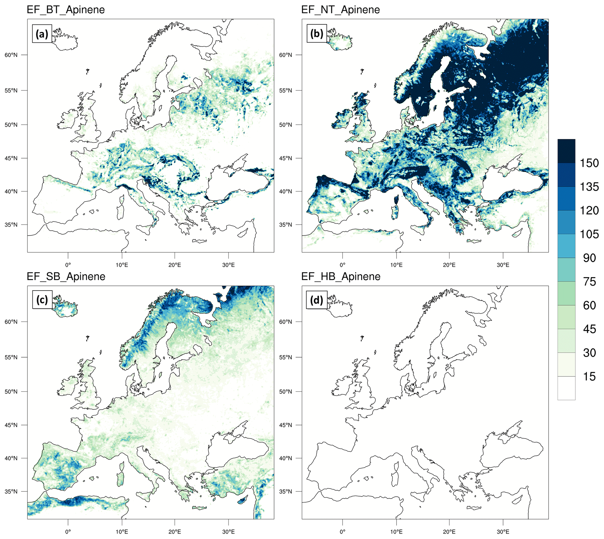
Figure 10 PFT-weighted emission factor (PFT emission factor and PFT percentage) (µg km⁻² h⁻¹) of α-pinene, computed for the month of August 2015 in Europe. The emission factor values used are from Table 2 (2.10 column). From the upper left map: (a) PFT-weighted emission factor of broadleaf trees (PFTP_BT), (b) needleleaf trees (PFTP_NB), broadleaf shrubs (PFTP_SB), and (d) grass and other (PFTP_HB).

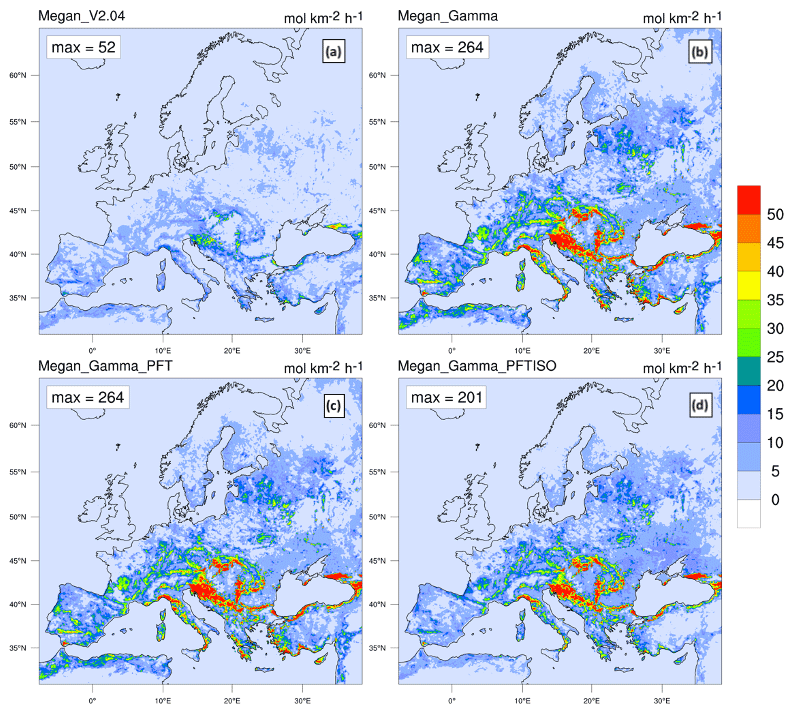
Figure 11 The spatial distribution of isoprene emissions (mol km⁻² h⁻¹) calculated as an average in the time period from 10 August 2015 at 00:00 UTC to 16 August 2015 at 00:00 UTC for the different MEGAN configurations, namely (a) the control simulation (M2.04), (b) activity factors (γ_i) updated (MG), (c) PFT emission factors updated (MGPFT), and (d) isoprene emission factors updated (M2.10).

Figure 12 The spatial distribution of α-pinene emissions (mol km⁻² h⁻¹) calculated as a weekly average (from 10 August 2015 at 00:00 UTC to 16 August 2015 at 00:00 UTC) for the different MEGAN configurations, namely (a) the control simulation (M2.04), (b) activity factors (γ_i) updated (MG), (c) PFT emission factors updated (MGPFT), and (d) isoprene emission factors updated (M2.10).

Figures 11 and 12 illustrate the spatial distribution of BVOC emissions calculated with different MEGAN configurations, respectively, for isoprene and α-pinene emissions as the weekly averaged emission flux (from 10 August at 00:00 UTC to 16 August 2015 at 00:00 UTC ). The updates to the MEGAN algorithm introduce a significant increase in both isoprene and α-pinene emissions. The areas with higher increases (from 15 to 50 mol km⁻² h⁻¹ for isoprene emissions; from 0.5 to 5 mol km⁻² h⁻¹ for α-pinene emissions) in emissions are the Balkan Peninsula, the Apennine Mountains (Italy), and part of the Black Sea coasts (Turkey and Georgia). The Iberian Peninsula and central–eastern Europe show minor differences, but these are still noteworthy (from 15 to 35 mol km⁻² h⁻¹ for isoprene; from 0.5 to 3.5 mol km⁻² h⁻¹ for α-pinene). The increase in emissions on the Balkan Peninsula, Italy, and the Black Sea coast is likely a result of the substantial increase in γ_LAI (Fig. S3), which contrasts with the decreased broadleaf PFT emission factor from 13 000 to 9000 µg m⁻² h⁻¹ (Table 2).

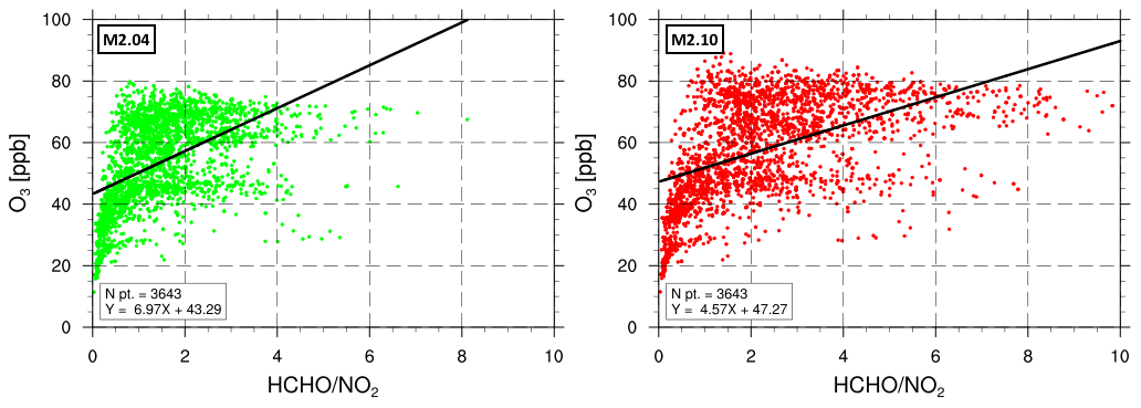
Figure 13 Scatter plot and linear regression of O₃ bias versus the ratio of HCHO $/$ NO₂ for the simulations M2.04 (green dots) and M2.10 (red dots). Each plot shows the number of ground-based monitoring observations (N pt.) from the AirBase database and the equation for the line of best fit (Y).

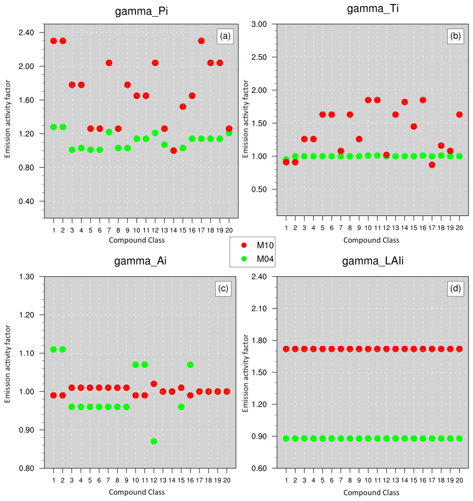
Figure 14 Emission activity factors (y axis, dimensionless) from M2.04 (M04) and M2.10 (M10) for different compound classes (1: isoprene, 2: myrcene, 3: sabinene, 4: limonene, 5: 3-carene, 6: t-β-ocimene, 7: β-pinene, 8: α-pinene, 9: other monoterpenes, 10: α-farnesene, 11: β-caryophyllene, 12: other sesquiterpenes, 13: 232-MBO, 14: methanol, 15: acetone, 16: carbon monoxide, 17: nitric oxide, 18: bidirectional VOC, 19: stress VOC, 20: other VOC). Each panel is for a different meteorological factor: (a) photosynthetic photon flux density (γ_P, GAMMA_P), (b) temperature (γ_T, GAMMA_T), (c) leaf age (γ_age, GAMMA_A), and (d) leaf area index (γ_LAI, GAMMA_LAI). The factors refer to the city of Genoa (Italy) on 13 August (12:00 UTC) 2015.

In Fig. 14a–d, a comparison is presented between the M2.04 run (green points) and the M2.10 (red points) emission activity factors γ_P, γ_T, γ_age, and γ_LAI for the city of Genoa (Italy) on 13 August (12:00 UTC) 2015 (Figs. S3, S4, and S5 of the Supplement show the remaining emission activity factors, respectively, for Kyiv, Porto, and Zagreb). The new emission activity factors are substantially higher than those in MEGAN version 2.04. The PPFD gamma factor increases for isoprene from 1.25 in M2.04 to 2.3 in M2.10, which is 1.8 times greater, and for α-pinene from 1.0 to 1.2. While isoprene and other VOCs had little change in the temperature gamma factor (gamma_T), the γ_T factor increased from 1.0 for M2.04 to 1.6 for M2.10. The leaf age emission activity factor (gamma_A) changed < 10 % between M2.04 and M2.10, decreasing for isoprene and increasing for α-pinene. For all VOCs, the LAI gamma factor increased from 0.9 to 1.7, which has a substantial effect on the VOC emissions. Figure 15a–d show the total emission activity factors (i.e., gamma = gamma_P ⋅ gamma_T ⋅ gamma_A ⋅ gamma_LAI) for each city between version 2.04 (M2.04, green points) and version 2.10 (M2.10, red points) of the MEGAN equation for 12:00 UTC on 13 August 2015. Compared to the M2.04 run, the emission activity values have increased significantly in the M2.10 run even considering the total value with an average value of about 3 (Genoa and Zagreb), 0.6 (Porto), and 0.45 (Kyiv). Naturally, the increase in total values derives from the variation of single activity factors; for example, in Genoa the values double by updating the code from M2.04 to M2.10, particularly for γ_P, γ_T, and γ_LAI (Fig. 15). Zagreb shows a similar trend. The gap relative to Kyiv and Porto is instead mainly due to γ_T and γ_LAI, while the PPFD activity factor (γ_P) has a lower influence.

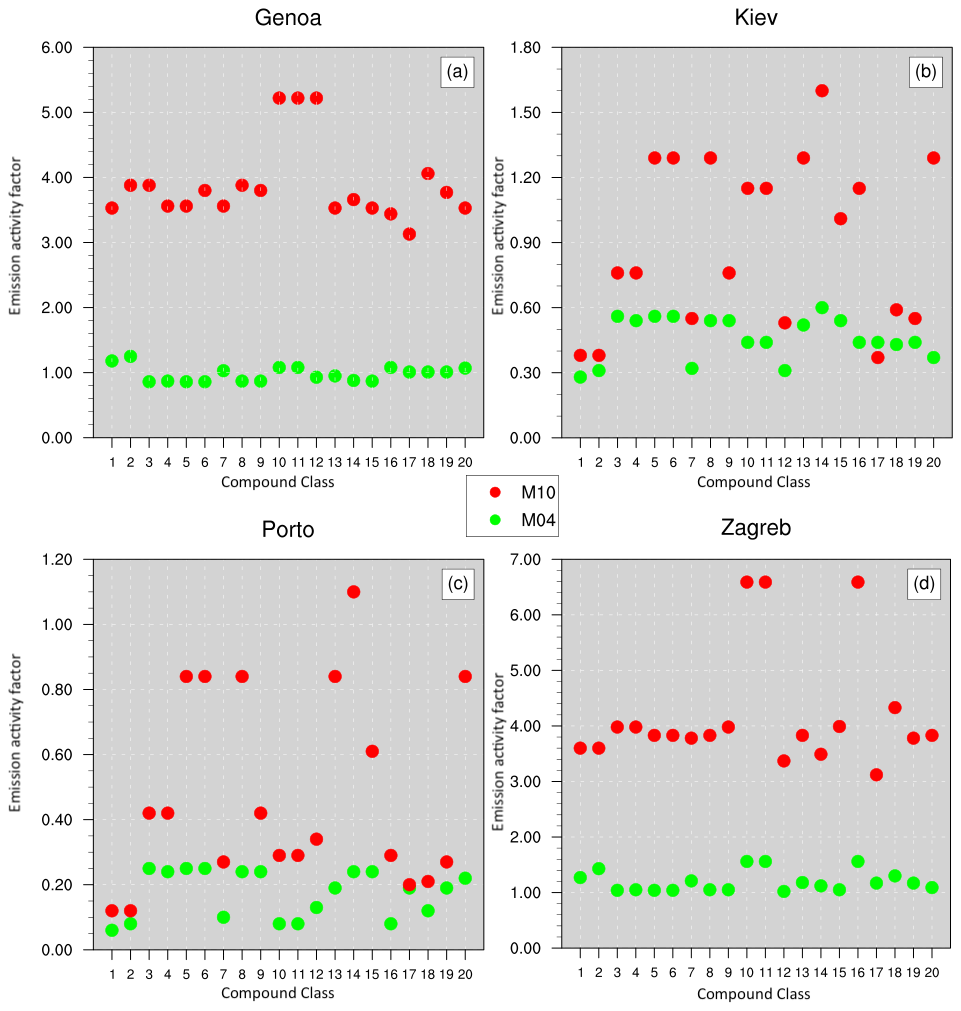
Figure 15 Total emission activity factors (y axis, dimensionless) from M2.04 (M04) and M2.10 (M10) runs for different compound classes (i.e., 1: isoprene, 2: myrcene, 3: sabinene, 4: limonene, 5: 3-carene, 6: t-β-ocimene, 7: β-pinene, 8: α-pinene, 9: other monoterpenes, 10: α-farnesene, 11: β-caryophyllene, 12: other sesquiterpenes, 13: 232-MBO, 14: methanol, 15: acetone, 16: carbon monoxide, 17: nitric oxide, 18: bidirectional VOC, 19: stress VOC, 20: other VOC). Each panel is for a different city: (a) Genoa (Italy), (b) Kyiv (Ukraine), (c) Porto (Portugal), and (d) Zagreb (Croatia) on 13 August 2015 (12:00 UTC).

4.1.3 Evaluation of trace gas compounds

About 3000 air quality monitoring stations in 34 countries across Europe were analyzed from the AirBase database (https://www.eea.europa.eu/data-and-maps/data/aqereporting-8, last access: 2 February 2018) for O₃ and its precursors (i.e., CO and NO₂). Since discrepancies between modeled and measured values might be related to the type and location of a measurement station, the selected stations were also disaggregated into categories based on the study done by Henne et al. (2010), which includes a more complete analysis of the surroundings of each station. The alternative classification provides three station class types: urban, suburban, and rural surface stations. Urban means a continuously built-up urban area (buildings with at least two floors), and the built-up area is not mixed with non-urbanized areas; suburban area is largely built-up urban area, with contiguous settlement of detached buildings of any size and the built-up area mixed with non-urbanized areas (e.g., agricultural, lakes, and woods). All areas that do not meet the criteria for urban or suburban areas are defined as rural areas.

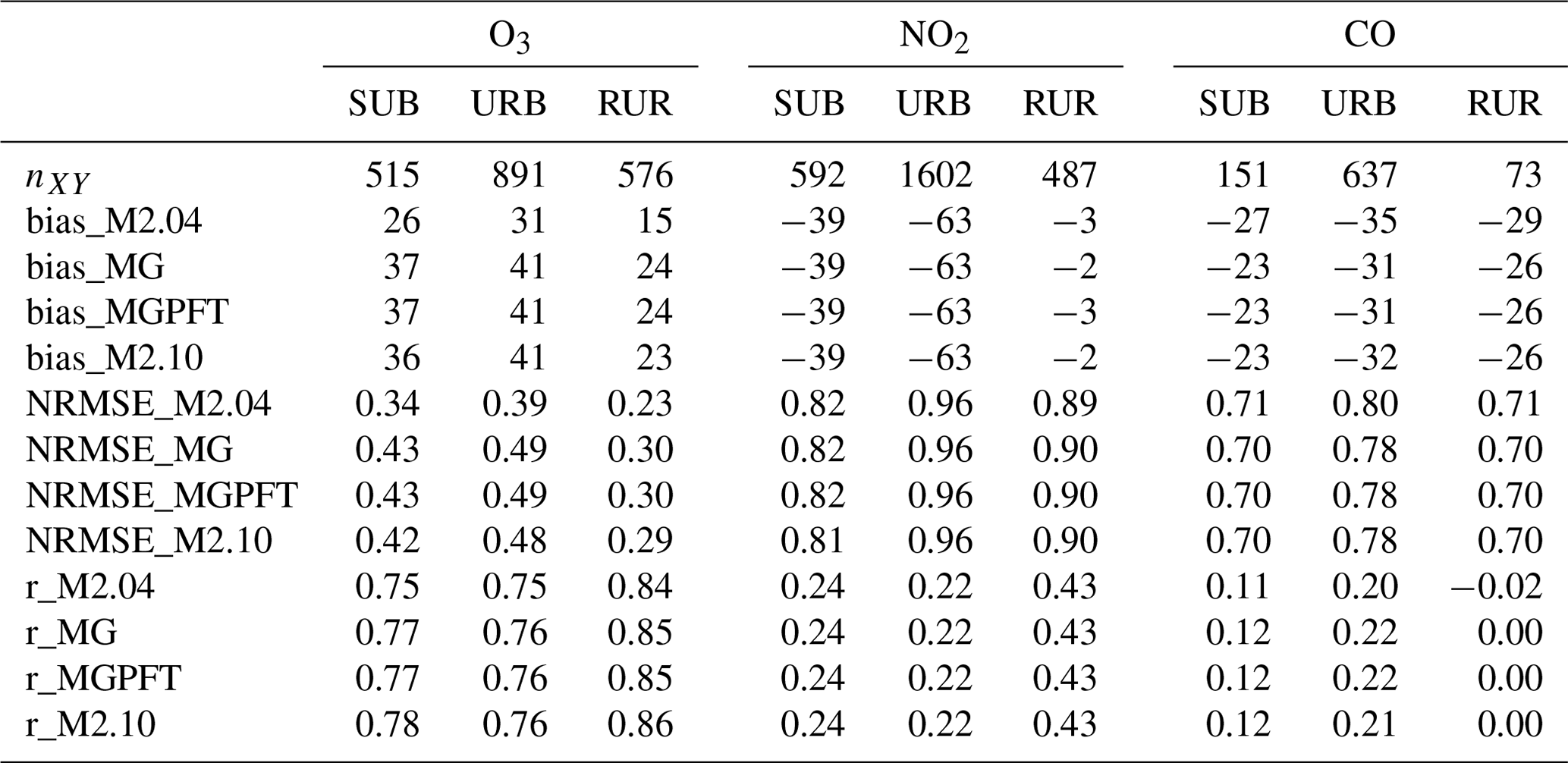
For each station the weekly mean of the concentrations was calculated for the daytime hours from 07:00 to 18:00 UTC. The mean bias, the normalized root mean square error, and the correlation coefficient were calculated between the measured and simulated compounds (i.e., O₃, NO₂, and CO) for the different station classes (i.e., urban, suburban, and rural stations). Regardless of the monitoring station type (i.e., urban, suburban, and rural), the M2.10, MG, and MGPFT runs show similar statistics for ozone, with a consistent overestimation of its concentrations compared to M2.04. For each model run and type of station, comparison between modeled and measured ozone concentrations shows positive mean bias values in the range 15 %–41 % (Table 5). The ozone concentrations in rural areas present the lowest biases (M2.04 = 15 %, MG = MGPFT = 24 %, and M2.10 = 23 %), while the highest biases are from the urban scenario (M2.04 = 31 %, M2.10 = 40 %, and MG = MGPFT = 41 %). The MEGAN updates increase the mean biases of ozone concentrations by about 10 % regardless of the type of station considered. The changes to the MEGAN algorithm (i.e., MG, MGPFT, and M2.10 runs) have a small to negligible effect on modeled NO₂ and CO, with only CO having an increase of 2 %–4 % from the control simulation M2.04 compared to the other model runs (Table 5).

Table 5 Summary of the statistics between predicted and measured O₃, NO₂, and CO concentrations from the AirBase dataset (intended as the daytime hour weekly mean from 10 August 2015 at 00:00 UTC to 16 August 2015 at 00:00 UTC), namely the (a) normalized mean bias (bias – %), (b) normalized root mean square error (NRMSE – dimensionless), (c) the correlation coefficient (r – dimensionless), and the relative number of points analyzed (n_XY). Values are shown according to the different station areas of suburban (SUB), urban (URB), and rural (RUR), as well as the different WRF-Chem model runs (control simulation – M2.04, activity factors updated – MG, PFT emission factors updated – MGPFT, and the isoprene emission factors updated – M2.10).

For the different model runs ,anthropogenic, biogenic, and biomass burning NO_x emissions did not vary. Specifically, soil NO_x emissions were evaluated with MEGAN as a function of environment variables (i.e., temperature and vegetation types) that were the same for each model run. Therefore, no substantial changes were noted for the NO_x concentration levels for the different model runs. Recent studies regarding the effects of NO_x soil emissions on O₃ levels in California (USA) (Sha et al., 2021) and Europe (Visser et al., 2019) have pointed out that NO_x levels were underestimated with large biases because of the low NO_x soil emissions estimated with WRF-Chem/MEGAN. NO_x soil emissions are important for both the tropospheric NO_x budget and surface O₃ level (Sha et al., 2021). Considering that the model runs with increases in BVOC emissions showed higher O₃ levels, it is likely that the O₃ formation was not NO_x-limited. MEGAN estimates carbon monoxide emissions as a biogenic emission class, unlike NO_x soil emissions. Higher CO emissions were noted for the MG simulation compared to the control run (M2.04) because of the changes in emission activity factors (γ_i). As reported in Table 2, the CO emission factor differs between MG and MGPFT runs, with a lower value for MGPFT (600 CO µg m⁻² h⁻¹) compared to MG (1000 CO µg m⁻² h⁻¹). Moreover, the higher emission activity factor and lower CO emission factor in MGPFT compared to the control run resulted in only slight differences in CO levels between the two runs. Therefore, the different model runs show slight variations in CO levels.

Since changes to NO₂ and CO emissions and mixing ratios were small, the increase in the O₃ biases may be due to the increased biogenic VOC emissions. Formaldehyde (HCHO), which is a product of BVOC chemistry, can play an important role in O₃ formation. The HCHO to NO₂ ratio is often used to show the role of VOCs in O₃ production, with higher HCHO to NO₂ ratios indicating higher O₃ production (e.g., Souri et al., 2020). A comparison of HCHO to NO₂ ratios for M2.04 and M2.10 simulations (Fig. 13) shows that in general HCHO $/$ NO₂ is higher in the M2.10 simulation than the M2.04 simulation, suggesting that the higher BVOC emissions promoted more HCHO formation and subsequently O₃ formation.

There are strong positive correlations between modeled and observed O₃ concentrations, with slightly higher values of the correlation coefficient for MG, MGPFT, and M2.10 compared to M2.04. The ozone correlation coefficients are higher for the rural monitoring stations (O_3-rural= 0.84–0.86), followed by the urban and suburban stations with values of about 0.75. Comparisons between modeled and measured ozone concentrations at rural background monitoring stations limit the influence of the model resolution (Table 5) (Jiang et al., 2019). Table 5 presents nitrogen dioxide correlation coefficient values in the range of 0.22–0.43, again with the lowest values for the urban and suburban stations, and the correlation coefficients for CO, with low values (−0.02 to 0.22) for all the types of monitoring stations. There are no remarkable modifications with the different MEGAN update simulations: O₃ and CO have an increase of about 0.01–0.02 from the control run (M2.04) to the MEGAN updates simulations (MG, MGPFT, and M2.10), while the nitrogen dioxide correlation coefficient has literally no variations between the different MEGAN updates. Figure 16 displays scatter plots and regression lines having on the ordinate axis the observed (AirBase dataset) concentrations and on the abscissa axis the simulations performed (i.e., M2.04 and M2.10 runs). The concentrations of O₃, NO₂, and CO observed and modeled support the statistical analysis of biases, RMSEs, and correlation coefficients.

Figure 16 Scatter plot and linear regression for the simulations M2.04 (M04 – a, green dots) and M2.10 (M10 – b, red dots) against the observed (AirBase dataset) concentrations (µg m⁻³) of (1) ozone, (2) nitrogen dioxide, and (3) carbon monoxide. Each plot shows the number of points recorded (N pt.) and the equation for the line of best fit (Y). The values shown are the 8 h daytime average weekly mean from 10 August 2015 at 00:00 UTC to 16 August 2015 at 00:00 UTC.

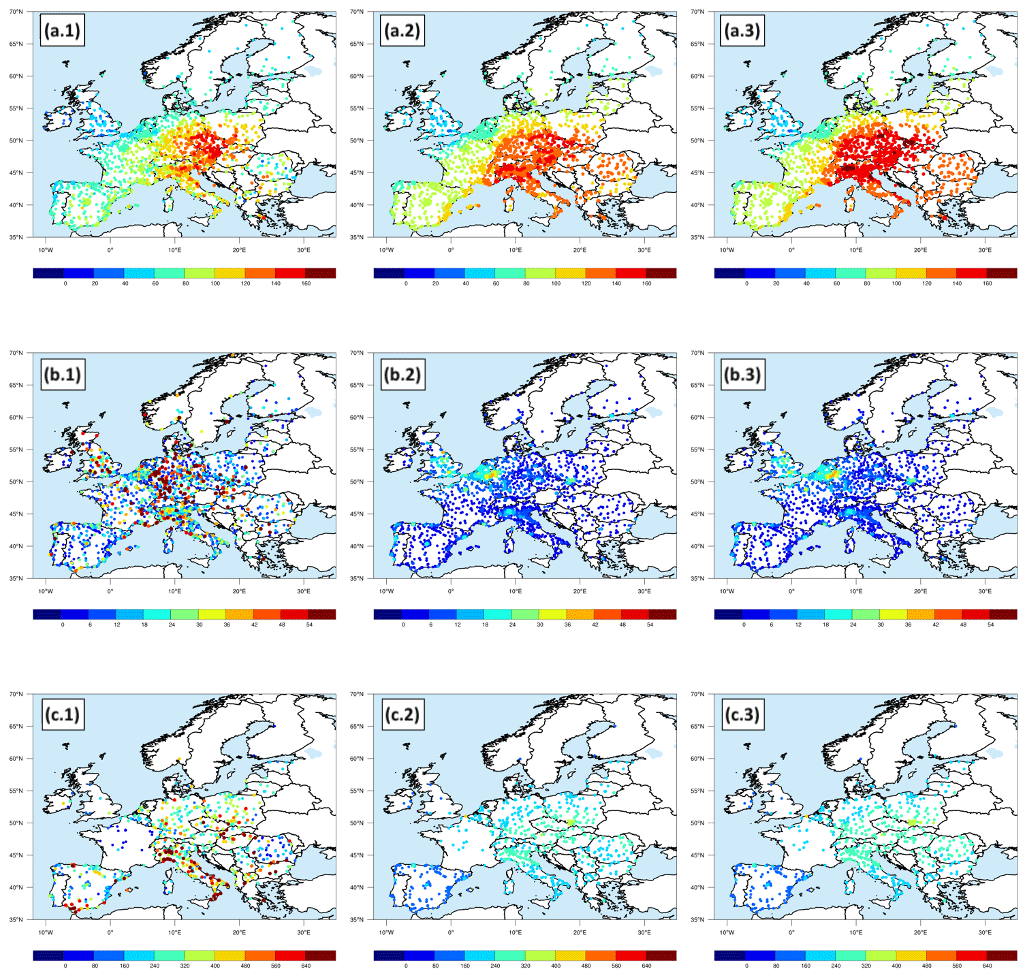
Figure 17 Comparison between the (1) AirBase dataset of the mean daytime (07:00–18:00,UTC), (2) control simulation (M2.04 run), and (3) M2.10 run concentrations with all the MEGAN code updates of (a) O₃, (b) CO, and (c) NO₂ over the period from 10 August 00:00 UTC to 16 August 00:00 UTC (2015).

To learn how the spatial variation compares between observed and predicted trace gases, maps of mean daytime (07:00–18:00 UTC) concentrations of O₃, CO, and NO₂ (Fig. 17) are examined for both the M2.04 control simulation and the M2.10 run with all the MEGAN code updates included. The spatial distribution of modeled ozone concentrations depicts the observed values well. However, the overestimation of the O₃ concentrations compared to the AirBase data is about 20 µg m⁻³ (about 10 ppb) and up to about 40 µg m⁻³ (about 20 ppb) for the M2.04 and M2.10 simulations, respectively. The overestimation is visible for most of Europe irrespective of the measured levels of O₃ concentration, but it is more evident in central Europe (France, Germany, Switzerland, Austria, and northern Italy) and the southern coast of the Iberian Peninsula. The results here contrast with those by Jiang et al. (2019), who found modeled ozone using the BVOC emission input from MEGAN v2.1 to be overestimated at low mixing ratios (20–50 ppb) and generally underestimated at mixing ratios above 50 ppb irrespective of the region of Europe considered. The NO₂ (Fig. 17b) concentration spatial distribution is not well represented by WRF-Chem, especially in northern Europe (i.e., England, Belgium, Netherlands, and northern Germany), northern Italy, and northeastern Spain. There is a large underestimation of NO₂ by the model in central Europe, where the difference is a factor of 10 (from 5 to 50 µg m⁻³ – approximately from 2.5 to 5 ppb). This may be due to the lack of updated anthropogenic emissions as the EDGAR-HTAP emissions (Janssens-Maenhout et al., 2011) represent 2010 not 2015, which impacts the nitrogen oxides that are mainly emitted from anthropogenic sources (e.g., road traffic), or due to the 12 km grid spacing in WRF-Chem not resolving high concentrations in urban locations.

The WRF-Chem model underestimates CO concentrations by a factor of 2 (from 240 to 500 µg m⁻³ – approximately from 210 to 435 ppb) for most of the stations measured (Fig. 17c), with the measured CO spatial distribution having no definite geographic pattern. The difference between measured and modeled CO concentrations is more evident across Italy, the south of Spain, Poland, and the Czech Republic. The magnitude of the gap in eastern Europe could be a sign that the model biomass burning emissions (FINN emissions – Wiedinmyer et al., 2011) cannot represent an overview of the situation well. Figure S6 shows a comparison between weekly average CO concentrations evaluated with the M2.10 run (Fig. S6a) and a simulation with the same model setup with no biomass burning emissions (Fig. S6b – “M2.10_noFINN”). The difference between the two simulations is clear in eastern Europe; without including the biomass burning emissions the CO concentration decreases from 240–320 to 160–240 µg m⁻³ (209–280 to 140–209 ppb). This indicates the presence of wildfire in that area, which is captured by both the AirBase dataset and the model but not sufficiently represented by biomass burning emissions and their computation in WRF-Chem. NO₂ concentrations are also affected by the biomass burning emissions (Fig. S7) but not as strongly as the CO concentrations. In general, the NO₂ differences between the M2.10 run (Fig. S7a) and the simulations with no biomass burning emissions (Fig. S7b – “M2.10_noFINN”) are about 5 µg m⁻³. Moreover, the CO and NO₂ concentrations do not show differences in spatial resolution and concentration magnitude between the MEGAN update simulations (Fig. 17).

4.2 Southeastern US case study

Since the southeastern US case study encompasses the NOMADSS field campaign, simulated biogenic VOCs and other trace gases can be evaluated. The MEGAN code updates are compared with the NOMADSS NCAR C-130 flight measurements to investigate the ability of the M2.04 and M2.10 simulations to depict the BVOC composition in the boundary layer.

4.2.1 Evaluation of trace gas compounds

Figure 18 shows the altitude of the flight, the temperature, and the mixing ratios of isoprene, methacrolein (MACR), methyl vinyl ketone (MVK), and ozone measured during the 5 June 2013 (14:00–21:00 UTC; 09:00–16:00 US central daylight time) flight (Fig. 18). Similar figures for flights on 3, 8, 12, and 14 June are shown in Figs. S8 to S11. Isoprene, MACR, and MVK were measured by a trace organic gas analyzer (TOGA), which is a fast online gas chromatograph–mass spectrometer (GC–MS) with a measurement frequency of approximately one 30 s sample every 2 min (Apel et al., 2003). Uncertainties of isoprene, MACR, and MVK are reported to be 15 %, 20 %, and 20 % of the measured mixing ratio, respectively.

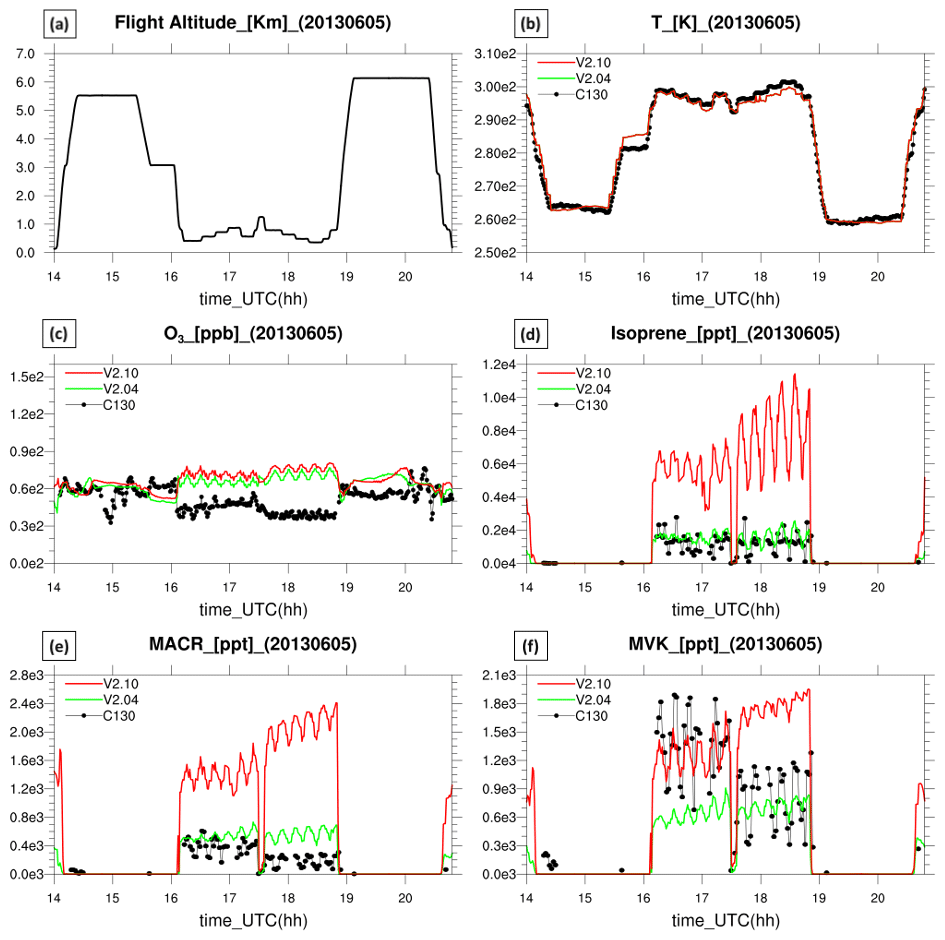
Figure 18 The flight altitude (a – km), temperature (b – K), and concentration of isoprene (c – ppb), methacrolein (MACR) (d – ppb), methyl vinyl ketone (MVK) (e – ppb), and ozone (f – ppb) for the second NOMADSS flight (rf02). The black line shows the C-130 aircraft measurements, and the green and red lines indicate the WRF-Chem model results using MEGAN version 2.04 (M2.04 run) and MEGAN updated to version 2.10 (M2.10 run), respectively. In panel (b) the green line is not shown since it is overlapped by the red line; they have identical values.

To explore the planetary boundary layer (PBL) ozone evolution, we examine the 5 June flight measurements since these measurements have a clear time frame (Fig. 18a) (i.e., from 16:15–18:45 UTC or 11:15–13:45 US central daylight time) when the aircraft was lower than the PBL height as it was flying near the Texas–Louisiana border (Fig. 3). Comparison of M2.04 and M2.10 simulations to aircraft observations shows that isoprene (Fig. 18c) mixing ratios agree well with measured isoprene for the M2.04 simulation but are overpredicted by up to 10 ppbv in the PBL. In response, MACR (Fig. 18d), a product of isoprene (Table S2 in the Supplement), is also overpredicted by the M2.10 simulation by up to a factor of 4, while MACR is either well-predicted or overestimated by up to a factor of 2 by the M2.04 simulation. MVK (Fig. 18e), an isoprene-dependent compound, has the opposite trend. That is, MVK flight-track measurements are more similar to the M2.10 run than the M2.04 simulation. In response to the higher isoprene, ozone mixing ratios (Fig. 18f) are affected, with MEGAN v2.04 results showing more similarity to measurements than the M2.10 simulation, which generally overpredicts ozone by 10–20 ppbv. Table S3 shows a statistical analysis of the model–observation normalized root mean square errors, correlations, and biases. As shown in the figures, the inclusion of updates from M2.04 to M2.10 tends to worsen the agreement with observations.

Often, CTMs tend to significantly overestimate surface ozone in the US (Brown-Steiner et al., 2015; Fiore et al., 2009; Lin et al., 2008). Recent studies have shed light on modeling surface ozone in the southeastern US (Travis et al., 2016; Schwantes et al., 2020; Cuchiara et al., 2020). Travis et al. (2016) investigated the main driving factors for the overestimation of modeled surface O₃ concentrations in the southeastern US by comparing CTM (i.e., Geos-Chem) predictions with multiplatform observations. These authors observed that a correction to the high-biased NO_x emissions led to better matching modeled and measured O₃ concentrations in both the PBL and the free troposphere. Cuchiara et al. (2020) investigated the interactions between cloud microphysics and the convective transport of soluble O₃ precursors from the PBL to the upper troposphere. These authors applied a 50 % reduction to the biogenic isoprene emission calculated with MEGAN v2.04 for WRF-Chem 3.9.1 based on the bias observed by previous studies in the US southeast. A comprehensive study by Schwantes et al. (2020) dealt with a more detailed description of isoprene and terpene chemistry for modeling surface ozone with CAM-chem during the summer 2013 time period. Based on sensitivity tests, Schwantes et al. (2020) observed that the more detailed isoprene chemistry representation improved agreement with the surface ozone daily max 8 h average values. Further, a paper by Ryu et al. (2018) clarifies the effect of cloud prediction on ozone: having clouds in the right place at the right time also improved ozone predictions. Nevertheless, for our study this is likely not the cause, and the ozone overprediction is mainly due to the isoprene emission changes. According to large-eddy simulations (Kim et al., 2016; Li et al., 2016; Ouwersloot et al., 2011) and measurement–model analysis (Kaser et al., 2015) the effects of the physical separation of isoprene and OH in the PBL depends on chemistry–turbulence interactions and scale-dependent heterogeneity of isoprene emissions, with potential implications for CTMs. The differences observed between measured and modeled isoprene mixing ratios along flight tracks may depend on the complex interaction between chemical reactions involving isoprene and turbulence within the PBL (Zhao et al., 2016). However, aircraft measurements generally take place under weather conditions and boundary layer heights scarcely affected by boundary layer mixing phenomena (Travis et al., 2016). Therefore, differences between modeled and aircraft data, which were observed in the present study, likely do not depend on simulated values of boundary layer meteorological variables.

5 Conclusions

To compare different updates to MEGAN v2.04 introduced by G12 to MEGAN v2.1 in simulating biogenic volatile organic compound (BVOC) emissions, two case studies were performed in two different domains (i.e., Europe and the southeastern United States). A sensitivity study on BVOC emissions was performed for a high-ozone episode in August 2015 in Europe considering a control run with MEGAN v.2.04 (i.e., M2.04) and the (i) update of the emission activity factors (i.e., MG), (ii) update of the emission factor values for each plant functional type (PFT) (i.e., MGPFT), and (iii) the assignment of the emission factor by PFT to isoprene (i.e., M2.10).

Comparisons between modeled and surface measured (AirBase database) ozone concentrations showed values of the correlation coefficients in the range from 0.78 to 0.86, with higher values for the rural monitoring stations compared to the urban and suburban ones. Correlation coefficients were higher in the M2.10 run compared to the M2.04 simulation. Moreover, the spatial distribution of modeled O₃ concentrations represented the observed values well, regardless of the simulations considered (M2.04, MG, MGPFT, and M2.10). However, magnitude differences were observed in both M2.04 and M2.10 simulations, with an overestimation of the O₃ concentrations compared to the AirBase data by about 20 µg m⁻³ (10 ppb) and up to about 40 µg m⁻³ (20 ppb), respectively. For the southeastern United States case study, modeled BVOC emissions were evaluated against aircraft measurements to investigate the performance of M2.04 and M2.10 runs in depicting the BVOC dynamics in the planetary boundary layer (PBL). Measurements of isoprene, two products of isoprene oxidation (i.e., methacrolein and methyl vinyl ketone), and ozone were taken in five of the research flights under the Southern Oxidant and Aerosol Study in June 2013. To analyze the PBL ozone evolution, flight measurements were considered when the flight-track height was lower than the PBL height; this showed that the M2.04 simulation better represented the flight-track isoprene mixing ratios than the M2.10 simulation. Each of the five research flights examined showed an M2.10 overestimation of isoprene mixing ratios up to a factor of 5. Comparisons between measured and modeled methacrolein and ozone reflected the isoprene comparison, with M2.04 results more similar to flight-track measurements than the updated M2.10 simulation. Methyl vinyl ketone showed an opposite trend to the isoprene one, with the M2.10 results more like the flight-track measurements than the control simulation.

In summary, the MEGAN updates (M2.10) generate substantially higher emissions of BVOCs by factors of 2 or more. For both situations modeled here, better agreement with observations is obtained using the older emissions (M2.04). Mainly, the simulations with updated emissions incurred larger biases in ozone measured across Europe and overpredicted the concentrations of BVOCs and their oxidation products observed directly during aircraft flights in the southeastern US. Both comparisons showed that BVOC emissions are better represented in M2.04 than in M2.10, suggesting further improvements are needed. These improvements should include increasing the number of PFTs from 4, used in this study, to 15, used in G12, and adding effects of the canopy and stress factors (Zhang et al., 2021), which are part of MEGAN v3. We also suggest further tests at different grid spacing so that vegetation variability and emission factors can be assessed. While we note substantial differences between M2.04 and M2.10 simulations, other factors in the WRF-Chem simulations could have affected the model evaluation. These other factors include underestimations of CO and NO₂ affecting the comparison with O₃ over Europe. Accurate anthropogenic and biomass burning emissions are also necessary for future evaluation. Cloudiness can directly affect not only biogenic emissions, but also photolysis rates, which impacts the ozone production (e.g., Ryu et al., 2018). Evaluation of the chemistry can also be aided by comparing WRF-Chem model results with satellite observations. For example, formaldehyde satellite measurements have been used to infer isoprene emissions (Curci et al., 2010). We lastly advocate for continued field measurements to refine emission factors with various vegetation types across the globe and experiments to better characterize the emission activity factors.