the Creative Commons Attribution 4.0 License.
the Creative Commons Attribution 4.0 License.
 | 12 Aug 2022
Large-eddy simulations with ClimateMachine v0.2.0: a new open-source code for atmospheric simulations on GPUs and CPUs
Yassine Tissaoui
Simone Marras
Zhaoyi Shen
Charles Kawczynski
Simon Byrne
Kiran Pamnany
Maciej Waruszewski
Thomas H. Gibson
Jeremy E. Kozdon
Valentin Churavy
Lucas C. Wilcox
Francis X. Giraldo
Tapio Schneider
We introduce ClimateMachine, a new open-source atmosphere modeling framework which uses the Julia language and is designed to be scalable on central processing units (CPUs) and graphics processing units (GPUs). ClimateMachine uses a common framework both for coarser-resolution global simulations and for high-resolution, limited-area large-eddy simulations (LESs). Here, we demonstrate the LES configuration of the atmosphere model in canonical benchmark cases and atmospheric flows using a total energy-conserving nodal discontinuous Galerkin (DG) discretization of the governing equations. Resolution dependence, conservation characteristics, and scaling metrics are examined in comparison with existing LES codes. They demonstrate the utility of ClimateMachine as a modeling tool for limited-area LES flow configurations.
- Article
(8963 KB) - Full-text XML
- BibTeX
- EndNote


Hybrid computer architectures and the need to exploit the power of graphics processing units (GPUs) are increasingly driving developments in atmosphere and climate modeling (e.g., Schalkwijk et al., 2012; Palmer, 2014; Schalkwijk et al., 2015; Marras et al., 2015; Abdi et al., 2017b, a; Fuhrer et al., 2018; Schär et al., 2020). The sheer computing power available on modern hardware architectures presents opportunities to accelerate atmosphere and climate modeling. However, exploiting this computing power requires re-coding atmosphere and climate models to an extent not seen in decades, and portable performance and scaling across different platforms remain difficult to achieve (Fuhrer et al., 2014; Balaji, 2021).
In this paper, we introduce ClimateMachine, a new open-source atmosphere model written in the Julia programming language (Bezanson et al., 2017) using the Julia Message Passing Interface (MPI) to provide a computational framework that is portable across CPU and GPU architectures. The use of Julia aims to increase accessibility and utility of ClimateMachine as a simulation tool. Julia, developed with the aim of bridging the gap between productivity (e.g., Python) and performance (e.g., Fortran) languages (Bezanson et al., 2018), is a strong candidate for an application such as atmospheric large-eddy simulations (LESs). Features such as package composability, GPU programming tools, and interactive programming interfaces contribute to its usability in scientific computing. Compilation time, incompatibilities between Julia MPI programs and interactive read–eval–print loops (REPLs), and the discovery of code issues during runtime due to Julia's dynamic typing are general drawbacks for new users of this language. Despite these drawbacks, a recent assessment by Lin and McIntosh-Smith (2021) further supports the suitability of Julia as a high-performance computing language. The atmospheric model presented here is designed to be usable across a range of physical process scales from large-eddy simulations (LESs) with meter-scale resolution to global circulation models (GCMs) with horizontal resolutions of tens of kilometers, as in a few other recent models (Dipankar et al., 2015). We focus on the LES configuration of ClimateMachine in this paper.
Since the pioneering work on turbulence in stratified flows by Lilly (1962), on horizontal subgrid-scale dissipation in GCMs by Smagorinsky (1963), and the subsequent extension of such models to LESs (Lilly, 1966), several models have been developed to improve the ability of LESs to model atmospheric turbulence: from the extensive work by Deardorff in the 1970s and 1980s (Deardorff, 1970, 1974, 1976, 1980), Moeng in the 1980s and beyond (Moeng, 1984; Moeng and Wyngaard, 1988; Sullivan et al., 1994; Moeng et al., 2003), to Stevens, Teixeira, Mellado, and others in the last 2 decades (Stevens et al., 2003, 2005; Savic-Jovcic and Stevens, 2008; Matheou et al., 2011; Pressel et al., 2015; Matheou, 2016; Matheou and Teixeira, 2019; Mellado, 2017; Mellado et al., 2018). LES results in canonical flows are sensitive to the fine details of the equations used to represent the flow dynamics, the viscous dissipation, the thermodynamics, and the numerical methods used to solve them (Ghosal, 1996; Chow and Moin, 2003; Kurowski et al., 2014), especially in the case of cloud simulations (Stevens et al., 2005; Siebesma et al., 2003; Schalkwijk et al., 2012, 2015; Schneider et al., 2019; Pressel et al., 2015, 2017).
One distinguishing aspect of the ClimateMachine LES is that it uses a nodal discontinuous Galerkin (DG) formulation to approximate the Navier–Stokes equations for compressible flow (Giraldo et al., 2002; Hesthaven and Warburton, 2008a; Giraldo and Restelli, 2008; Kopriva, 2009; Kelly and Giraldo, 2012; Giraldo, 2020). The DG method is a spectral-element generalization of finite-volume methods. It lends itself well to modern high-performance computing architectures because its communication overhead is low, enabling scaling on many-core processors including GPUs (Abdi et al., 2017b). Another important consideration within ClimateMachine is the use of total energy of moist air as a prognostic variable, ensuring energetic consistency of the simulations. We demonstrate that the ClimateMachine LES can be successfully used to simulate canonical LES benchmarks, including simulations of flows over mountains and different cloud and boundary layer regimes (e.g., Straka et al., 1993; Schär et al., 2002; Stevens et al., 2005).
In what follows, we describe the conceptual and numerical foundations and governing equations of ClimateMachine and demonstrate the model in a set of standard two- and three-dimensional benchmark simulations. Section 2 begins by highlighting the governing equations. Their numerical approximation through the DG representation is described in Sect. 3. Section 4 presents subgrid-scale models used in the LES to represent under-resolved flow physics, with results from key benchmarks presented in Sect. 5. Conservation properties are examined in Sect. 6, and performance on CPU and GPU hardware is described in Sects. 7 and 8, respectively. Section 9 contains closing remarks. Additional details about the model, boundary conditions, statistical definitions, and computer hardware are summarized in the Appendices.
2.1 Working fluid
The working fluid of the atmosphere model is moist, potentially cloudy air, considered to be an ideal mixture of dry air, water vapor, and condensed water (liquid and ice) in clouds. Dry air and water vapor are taken to be ideal gases. The specific volume of the cloud condensate is neglected relative to that of the gas phases (it is a factor of 103 less than that of the gas phases). All gas phases are assumed to have the same temperature and are advected with the same velocity . Cloud condensate is assumed to sediment relative to gaseous phases slowly enough to be in thermal equilibrium with the surrounding fluid.
The density of the moist air is denoted by ρ. We use the following notation for the mass fractions of the moist air mixture (mass of a constituent divided by the total mass of the working fluid).
-
qd: dry air mass fraction
-
qv: water vapor specific humidity
-
ql: liquid water specific humidity
-
qi: ice specific humidity
-
: condensate specific humidity
-
: total specific humidity
Because this enumerates all constituents of the working fluid, we have . In Earth's atmosphere, the water vapor specific humidity qv dominates the total specific humidity qt and is usually 𝒪(10−2) or smaller; the condensate specific humidity is typically 𝒪(10−4). Hence, water is a trace constituent of the atmosphere, and only a small fraction of atmospheric water is in condensed phases. The working fluid pressure is the sum of the partial pressures of dry air and water vapor such that , where Rd is the specific gas constant of dry air, and Rv is the specific gas constant of water vapor.
2.2 Mass balance
Moist air mass satisfies the conservation equation:
Moist air mass is not exactly conserved where precipitation forms, sublimates, or evaporates, where water diffuses, or where condensate sediments relative to the gas phases (Bott, 2008; Romps, 2008). The right-hand side involves the local source and/or sink of water mass owing to such nonconservative processes, which we take into account although it is small because water is a trace constituent of the atmosphere.
2.3 Total water balance
Total water satisfies the balance equation:
Here, the source–sink arises from evaporation or sublimation of precipitation and formation of precipitation. Diffusive fluxes of moisture are captured by . The effective sedimentation velocity of cloud condensate wc is defined such that
with wl and wi defined to be positive downward ( being the upward-pointing unit vector). The right-hand side of the total water balance equation is the same as the right-hand side of the mass balance in Eq. (1).
2.4 Momentum balance
The coordinate-independent form of the conservation law for momentum is
where I3 is the rank-3 identity matrix, Φ is the effective gravitational potential including centrifugal accelerations, τ is a viscous and/or subgrid-scale (SGS) momentum flux tensor, and Fu (typically with so that Fu represents a momentum sink) is any other drag force per unit mass that may be applied, for example, at the lower boundary. The term involving the planetary angular velocity Ω accounts for Coriolis forces. To improve numerical stability, we have factored out a reference state with a pressure pr(z) and density ρr(z) that depend only on altitude z and are in hydrostatic balance so that they satisfy
The tensor involving the diffusive flux of water on the right-hand side of Eq. (4) represents the momentum flux carried by water that is diffusing; this term is usually very small, but we take it into account.
2.5 Energy balance
The specification of a thermodynamic or energy conservation equation closes the equations of motion for the working fluid. We use the total specific energy, etot, as the prognostic variable. Total energy is conserved in reversible moist processes such as phase transitions of water.
Total energy satisfies the conservation law (Romps, 2008; Bott, 2008):
where the total specific energy etot is defined by
The constituents (dry air and moisture components) here are assumed to be moving with the same velocity u (that is, we neglect, as is common, the diffusive and sedimentation fluxes of water in the kinetic energy). The constituents are also assumed to be in thermal equilibrium at the same temperature T so that the specific internal energy of moist air is the weighted sum of the specific energies of the constituents dry air (Id), water vapor (Iv), liquid water (Il), and ice (Ii):
with
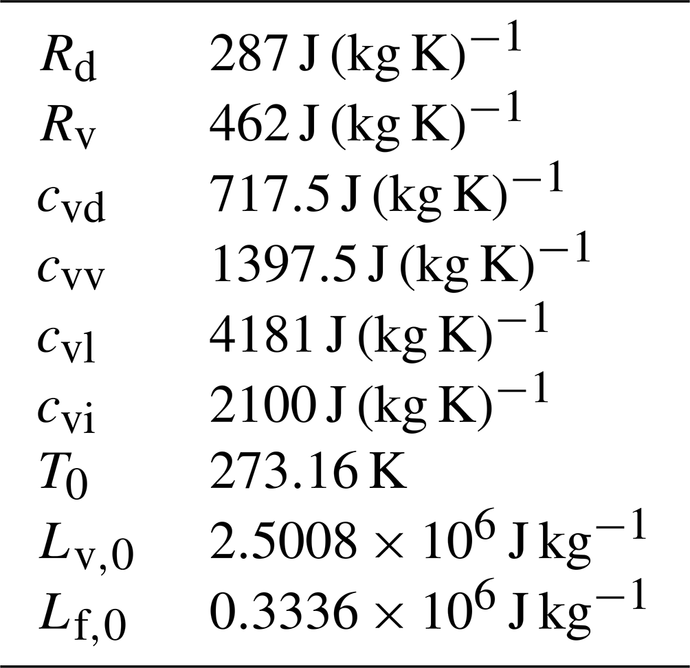
Here, cvk for k∈{d, v, l, i} represents isochoric specific heat capacities for the appropriate species denoted by k; they are taken to be constant. The reference specific internal energy Iv,0 is the difference in specific internal energy between vapor and liquid at the arbitrary reference temperature T0; Ii,0 is the difference in specific internal energy between ice and liquid at T0 (Romps, 2008). The reference internal energies are related to specific latent heats of vaporization and fusion, Lv,0 and Lf,0, at the reference temperature T0 through
The values of the thermodynamic constants we use are listed in Table 1.
Furthermore, the flux FR is the radiative energy flux per unit mass; J is the conductive energy flux per unit mass, and D is the specific enthalpy flux associated with the diffusive flux of water:
The flux u⋅ρτ is the energy flux associated with the viscous and/or SGS turbulent momentum flux; Q is any internal energy source (e.g., external diabatic heating). The flux
represents the downward energy flux due to sedimenting condensate.
The terms involving ρC(qj→qp) (j∈{ v, l, i }) represent the loss of internal and potential energy of moist air masses owing to precipitation formation; the kinetic energy loss is neglected, consistent with the neglect of the source and/or sink associated with precipitation formation in the momentum balance in Eq. (4). Additional energy sinks involve the energy loss owing to heat transfer from the working fluid to precipitation as it falls through air and possibly melts at the freezing level (Raymond, 2013); the associated energy sources and sinks are generally provided by a microphysics parameterization and are subsumed in the term M.
2.6 Equation of state
Pressure p is calculated from the ideal gas law:
where Rm is the gas “constant” of moist air,
with the ratio of the gas constants of water vapor and of dry air .
2.7 Saturation adjustment
Gibbs' phase rule states that in thermodynamic equilibrium, the temperature T and liquid and ice specific humidities ql and qi can be obtained from the three thermodynamic state variables density ρ, total water specific humidity qt, and internal energy I. Thus, the above equations suffice to completely specify the thermodynamic state of the working fluid given ρ, qt, and I, with the latter obtained from the total energy via its definition in Eq. (6).
Obtaining the temperature and condensate specific humidities from the state variables ρ, qt, and I is the problem of finding the root T of
where is the internal energy at equilibrium, when the air is either unsaturated and there is no condensate (qv=qt), or water vapor is in saturation and the saturation excess qt−qv is apportioned, according to temperature T, among the condensed phases ql and qi. We solve this nonlinear “saturation adjustment” problem by Newton iterations with analytical gradients (see Tao et al., 1989; Pressel et al., 2015). To obtain the saturation vapor pressure and derived functions needed in this calculation, we assume all isochoric heat capacities to be constant (i.e., we assume the gases to be calorically perfect); with this assumption, the Clausius–Clapeyron can be integrated analytically, resulting in a closed-form expression for the saturation vapor pressure (Romps, 2008).
This procedure allows the use of total moisture qt as the sole prognostic variable but confines the system to the assumption of equilibrium thermodynamics. Alternatively, using explicit tracers for the condensate specific humidities ql and qi allows non-equilibrium thermodynamics to be considered and mixed-phase processes to be explicitly modeled.
3.1 Space discretization
The governing equations are discretized in space via a nodal DG approximation. To describe the DG procedure, we recast the Eqs. (1)–(5) in divergence form as
where is an abstract vector of state variables, F1 contains the fluxes not involving gradients of state variables and functions thereof, F2 contains the fluxes involving gradients of state variables (e.g., diffusive fluxes), and 𝓢(Y) contains the sources.
The DG solution of Eq. (16) is approximated on the finite-dimensional counterpart Ωh of the flow domain Ω, which consists of non-overlapping hexahedral elements Ωe such that
where a superscript h indicates the discrete analog of a continuous quantity. By virtue of tensor-product operations allowed on hexahedral elements and the ability to rely on inexact quadrature when elements of order greater than 3 are utilized, high-order Galerkin methods are particularly attractive for operation-intensive solutions (Kelly and Giraldo, 2012). Within each element, the finite-dimensional approximation of Y(x,t) is given by the expansion
where (N+1)3 is the number of collocation points within the three-dimensional element of order N, and represents the interpolation polynomials evaluated at local point α inside element e.
From now on, the subscript or superscript e is omitted with the understanding that all operations are executed element-wise unless otherwise stated. Furthermore, the physical elements in the space are mapped to a reference element . The three-dimensional basis functions ψα result from the one-dimensional functions Li(ξ), Lj(η), and Lk(ζ) as the tensor product:
Each function L is a one-dimensional (1D) Lagrange polynomial defined on the 1D reference element . The Lagrange function evaluated at points i along the ξ direction within the element is
where ξi represents the N+1 co-located interpolation points along ξ. The polynomials Lj and Lk in the other two directions η and ζ are built in the same way. The N+1 interpolation points may be chosen in a variety of ways (Deville et al., 2002; Karniadakis and Sherwin, 1999); here we choose Legendre–Gauss–Lobatto (LGL) points (Giraldo and Restelli, 2008). The Kronecker δ property of the Lagrange polynomials is such that
in 1D, which, in three dimensions (3D), translates to
This allows us to reduce the operation count as follows. We construct the space and time derivatives as
By virtue of the 3D Kronecker δ property, the spatial derivatives of the basis functions appearing here are given by
Using this property reduces the operation count significantly since we only require 3N operations instead of the N3 operations otherwise needed to compute the derivatives at a given node (Abdi et al., 2017b).
The operators defined on the reference elements are mapped onto the physical space by means of the transformation
where and , and
is the inverse Jacobian of the transformation from physical space to the reference element.
The DG approximation of the differential Eq. (16) is constructed by multiplying, within each element, the equation by the test function ψα and then integrating over the element volume Ωe such that
where ψα within each element belongs to the function space of square integrable piecewise polynomials of order N (i.e., ψ∈L2). By definition, these functions are discontinuous across element boundaries; differentiability is not globally required but only within each element (Hesthaven and Warburton, 2008b). Integrating the divergence term by parts yields
where Ωe and Γe are the volume and boundary of each element, respectively, n is the outward-facing unit vector orthogonal to each element face, and is a numerical flux. The imposition of the numerical fluxes across element boundaries is the numerical mechanism that promotes continuity of the discontinuous solution across the elements. The numerical fluxes are calculated as the approximate solution to a Riemann problem across two neighboring elements. ClimateMachine currently implements the Rusanov (1961), Roe (1981), and Harten–Lax–van Leer contact (HLLC) (Toro et al., 1994; Harten, 1983) numerical fluxes. The Rusanov flux, for instance, is constructed as
where Y− is the state at the internal interface of element e, Y+ is the state at the external interface of e, and is an estimate of the maximum flow speed (e.g., the maximum eigenvalue of the Jacobian of the flux F1 with respect to the state variables, which is the speed of sound).
Because the second-order derivatives in ∇⋅F2 cannot be directly built with the weak variational formulation if a discontinuous function space is used (Bassi and Rebay, 1997), an auxiliary variable is introduced such that
which can then be discretized via DG as
Here, is approximated via centered flux like in Bassi and Rebay (1997). We also refer to Abdi et al. (2017b) for more details.
For algorithmic efficiency, inexact quadrature is used to calculate the integrals above. By virtue of inexact integration and of Eqs. (17), (19), and (24), the variational DG equations yield the semi-discrete matrix problem:
where represents interpolation weights. The algebraic details to obtain this expression can be found in Giraldo and Restelli (2008), where the s superscript indicates a value that is defined on the element boundary surface. The system (Eq. 31) is integrated on each element with respect to time.
In order to achieve good parallel scaling it is necessary to overlap communication and computation to the fullest extent possible. With DG (and all element-based Galerkin methods) this can be naturally achieved by splitting Eq. (31) into terms that arise from the approximation of volume integrals and surface integrals. All volume contributions can be calculated independently of element-to-element communication regardless of the order of the spatial approximation, as can surface integrals that are not on elements which share boundaries across MPI ranks. Thus, in the code, we start with Message Passing Interface (MPI) communication, do all volume calculations and surface calculations for elements not on boundaries shared across ranks, and then apply surface calculations for elements on the rank boundaries after communication operations have been completed. This approach makes DG naturally effective with respect to parallel computing as previously shown by, e.g., Müller et al. (2018) on CPUs and Abdi et al. (2017b) on GPUs. At high order, element-based Galerkin methods such as DG require fewer neighboring degrees of freedom than high-order finite-difference and finite-volume discretizations.
3.2 Time discretization
ClimateMachine provides a suite of time integrators consisting of explicit Runge–Kunge methods as well as low-storage (Carpenter and Kennedy, 1994; Niegemann et al., 2012), strong stability-preserving (Shu and Osher, 1988), and additive Runge–Kutta (ARK) implicit–explicit (IMEX) methods (Giraldo et al., 2013; Kennedy and Carpenter, 2019).
The benchmarks presented in this paper with isotropic grid spacing are run using the fourth-order 14-stage method of Niegemann et al. (2012), which has a large explicit time-stepping stability region. One of the benchmarks, however, uses a highly anisotropic grid, which benefits from the use of a 1D IMEX approximation; there we use a variant of the horizontally explicit, vertically implicit (HEVI) schemes by Bao et al. (2015). While 3D IMEX is also an option, its performance in terms of time to solution is ultimately limited by the availability of scalable 3D implicit solver algorithms.
The governing equations are resolved with the discretizations presented in Sect. 3. This leaves unresolved but dynamically significant scales on the computational grid that must be modeled with three-dimensional SGS models. We note that, while filtering over the grid volume is typically a formal requirement for LES variables, no explicit filter kernel is applied to the equations here. The resolution of the prognostic variables on a discretized grid constitutes an implicit filtering operation, with an equivalent length scale given by the grid resolution. In general, SGS fluxes are modeled as diffusive fluxes, which capture down-gradient transport of conservable scalar quantities assuming that mixing lengths are small compared with the scales over which the gradients of the scalars vary. We address the physical form of the diffusive flux components in Eqs. (1)–(5), following which we describe standard models of subgrid-scale turbulence available for use in ClimateMachine.
The diffusive turbulent stress tensor τ is represented in terms of the symmetric rate of strain tensor S such that
with
Here, νt is a turbulent viscosity tensor whose components are typically orders of magnitude larger than the molecular viscosity and are a function of the velocity gradient tensor.
The diffusive flux of total water specific humidity in Eq. (2) is modeled as
where 𝓓t is a turbulent diffusivity vector. The turbulent diffusivity 𝓓t is related to the turbulent viscosity tensor νt via the turbulent Prandtl number such that
where Prt takes a typical value of .
The unresolved flux of total enthalpy htot results in a diffusive subgrid flux term of the form
where J is the thermal diffusion flux analogous to the molecular conductive heat flux, and D is the energy flux carried by water vapor, defined in Eq. (11). For energetic consistency, we use the same turbulent diffusivity 𝓓t for moist enthalpy and water.
4.1 Smagorinsky–Lilly model
The turbulent eddy viscosity νt in the model by Lilly (1962) and Smagorinsky (1963) (SL henceforth) is defined by means of the magnitude of the rate of the strain tensor S, whose components are , according to
for ; Cs is a constant Smagorinsky coefficient usually within the range , and Δ is the LES filter width. Inside each hexahedral element of order N and side lengths along the x,y, and z directions, the effective grid resolution is , which is the average distance between two consecutive nodal points. We use an isotropic eddy viscosity tensor νt in LESs, with its components defined by Eq. (37). Similar eddy viscosity models can be found in other recent models of compressible atmospheric flows (e.g., Jähn et al., 2015; Shi et al., 2018).
4.2 Vreman eddy viscosity model
The SGS model developed by Vreman (2004) is of interest because of its robustness across flow regimes and because it has low dissipation near wall boundaries and in transitional flows. Its computational complexity is similar to the classical SL model. While the Vreman model is extensively used in engineering LESs, it is uncommon in atmospheric flows, for which a constant coefficient SL or the one-equation turbulent kinetic energy (TKE) model by Deardorff (1970, 1980) is the most common choice (see, e.g., Stevens et al., 2005).
The turbulent eddy viscosity of this model depends on first-order derivatives of velocities and is given by
where
Here, summation over repeated indices is implied, Cs is the constant Smagorinsky coefficient, and ui represents the components of the resolved-scale velocity vector so that ui,j is the velocity gradient tensor. The mixing lengths Δm can be determined as the grid spacing in the direction implied by subscript m; in this paper . Near-surface corrections to the characteristic length (e.g., Mason and Callen, 1986) have not been applied to either subgrid-scale model in the present work.
Richardson correction in stable regions of the atmosphere. To account for the atmospheric stability and, effectively, reduce turbulence generation to zero in stably stratified atmospheres, we multiply the eddy viscosity by the correction factor
where
Here, is a constant turbulent Prandtl number, and θv is the virtual potential temperature for a given specific humidity qt and specific liquid water content ql (see, e.g., Deardorff, 1980). This temperature is computed consistently with the moist phase partitioning (saturation adjustment) in the system and is therefore a reasonable measure of the effect of buoyancy on flow stratification. This is applied to both turbulence closures discussed in this paper.
4.3 Numerical stability
When high-order Galerkin methods are used to solve nonlinear advection-dominated problems, spurious Gibbs oscillations may affect the solution and need to be addressed. ClimateMachine provides a set of spectral filters, cut-off filters, and artificial diffusion methods to remove these oscillations. While filters may be effective, we found that stabilizing the LES solution by means of the SGS eddy viscosity alone is effective and robust; this is in agreement with results shown by Marras et al. (2015), Marras and Giraldo (2015), and Reddy et al. (2022) in the case of continuous Galerkin methods. Other methods of stabilizing numerical solutions are discussed by Light and Durran (2016) and Yu et al. (2015). This approach stems from the idea that under-resolved scales are responsible for the numerical oscillations observed in solutions through the introduction of unphysical artifacts in properties of the solution variables. Detailed analyses of the interactions of subgrid-scale models and filtering techniques with DG numerics in the context of atmospheric flows will be presented in a forthcoming paper.
We first demonstrate the convergence of the numerical solution to the Euler equations with an isentropic vortex advection problem. Following this, we demonstrate results from the ClimateMachine using standard benchmark problems including (1) dry rising thermal bubble in a neutrally stratified atmosphere, (2) dry density current, (3) hydrostatic and nonhydrostatic mountain-triggered linear gravity waves, (4) the Barbados Oceanographic and Meteorological Experiment (BOMEX), and (5) decaying Taylor–Green vortex in a triply periodic domain.
5.1 Advection of an isentropic vortex
To demonstrate convergence of the numerical solutions, we consider the two-dimensional dry isentropic vortex advection problem with fourth-order polynomials, consistent with the benchmark cases shown in the sections that follow. We consider the pure advection of a vortex in a domain with edge lengths L=0.1 m, with a vortex radius R=0.005 m. The initial velocity profile is given by
with a prescribed translational velocity u0=150 m s−1, translation angle , and a vortex speed vs=50 m s−1 so that the velocity perturbations are given by
The perturbations are computed with an offset coordinate given by
where x and y represent Cartesian coordinates, to ensure that the resulting functions are periodic. The initial temperature profile is given by
with a reference temperature of T∞=300 K, reference pressure p∞=105 Pa, and the corresponding density ρ∞ computed from the ideal gas law. The simulation time is given by . We consider fourth-order polynomials, with increasing refinement given by the addition of elements in the domain discretization, to generate the Euclidean distance between the initial state and the time-stepped solution state at s, as shown in Fig. 1. The results demonstrate consistent convergence across three numerical flux methods for element numbers ranging from 5–320. The convergence rate approaches 5 for the fourth-order polynomials considered in this study.
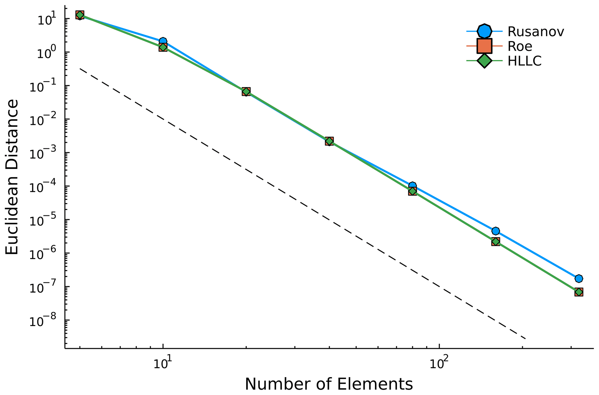
Figure 1Euclidean distance between initial and final solution vectors of the prognostic variables generated using Rusanov (octagons), Roe (squares), and Harten–Lax–van Leer contact (HLLC) numerical fluxes. Final solutions are evaluated at s based on a translational velocity of 150 m s−1. For each numerical flux method, we consider elements with fourth-order polynomials. The dashed line represents convergence.
Tests presented in Sect. 5.2–5.5 are executed in a 3D domain even when the problem is two-dimensional, in which case we have effectively zero tendencies in the third dimension; this setup is identified as 2.5D in what follows.
5.2 2.5D rising thermal bubble in a neutrally stratified atmosphere
A neutrally stratified atmosphere with uniform background potential temperature θ0=300 K is perturbed by a circular bubble of warmer air. The hydrostatic background pressure decreases with z as
in a domain m3. The perturbation is as defined in Ahmad and Lindeman (2007),
where , m, and θc=2 K. The initial velocity field is zero everywhere. Periodic boundary conditions are used along y, and solid walls with impenetrable, free-slip boundary conditions are used in the x and z directions. Detailed information on boundary conditions for all test cases is provided in Appendix A. Five runs are performed at effective uniform resolutions , 125, 62.5, and 31.25, and 15.625 m, with polynomial order N=4. Potential temperature θ and the two velocity components u and w are plotted at t=1000 s in Fig. 2 for the grid resolution of 15.625 m, which represents a reference solution for comparison with solutions at coarser resolutions. The value of the maximum potential temperature perturbation Δθmax and of the horizontal and vertical velocity components agree with the 125 m resolution results shown by Ahmad and Lindeman (2007). The grid dependence of the solution is shown in Fig. 3, where potential temperature is plotted for , 62.5, 125, and 250 m. While the solution is visibly more dissipative at coarser resolutions, the bubble's leading edge position (and hence propagation speed) is not sensitive to the grid resolution.
The SL and Vreman closures are used to model diffusive fluxes in this problem. The solutions show no discernible differences, and only the SL solution is shown. A visual comparison of the two becomes more meaningful when shear triggers mixing, which is shown for the density current test in Sect. 5.3. Although DG inherits an implicit numerical diffusion as an effect of the numerical flux calculation across elements, under-resolved advection-dominated problems still require a dissipation or filtering mechanism to preserve the solution's stability. In the case of Marras et al. (2015), a dynamically adaptive SGS model was used, whereas a Boyd–Vandeven filter (Boyd, 1996; Vandeven, 1991) was used by Giraldo and Restelli (2008).
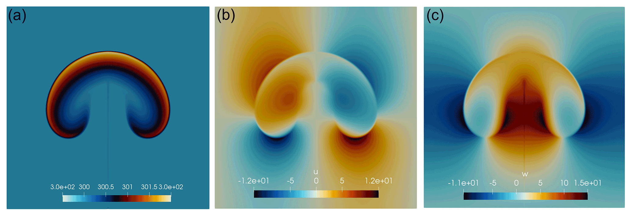
Figure 22.5D rising thermal bubble with effective resolution m and N=4. Panels depict (a) potential temperature θ, (b) horizontal velocity u, and (c) vertical velocity w at t=1000 s in km2.
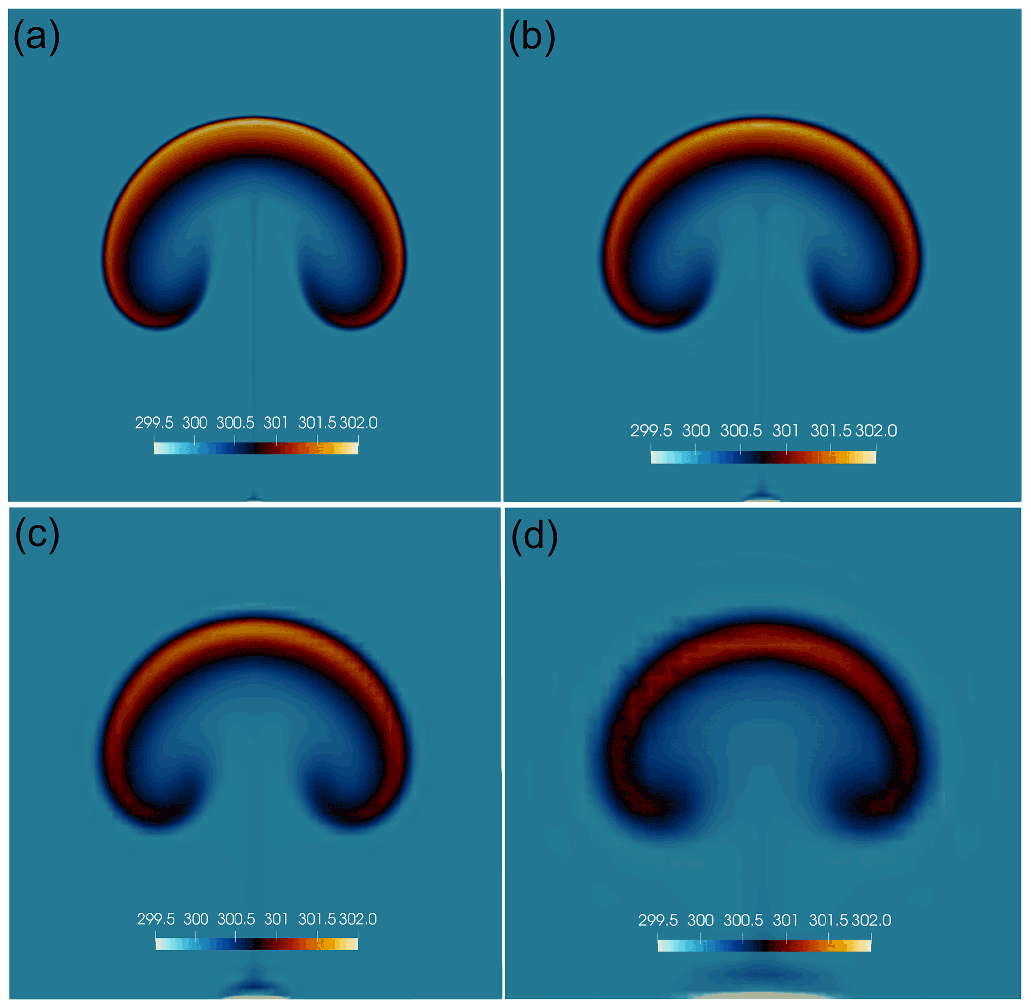
Figure 32.5D rising thermal bubble solution with N=4 at decreasing effective resolution. Grid convergence of potential temperature θ at four different resolutions to be compared against the 15.625 m resolution results shown in Fig. 2. (a) m, (b) 62.5 m, (c) 125 m, and (d) 250 m. Although the solution is visibly more dissipated at coarser resolution, the bubble's leading edge (and hence propagation speed) is not affected.
5.3 2.5D density current in a neutrally stratified atmosphere
The density current problem by Straka et al. (1993) is used to test the LES framework in a flow with Kelvin–Helmholtz instabilities. As for the rising thermal bubble, the background initial state is in hydrostatic equilibrium at uniform potential temperature θ0=300 K. A perturbation of θ centered on m and with radii m is given by the function
where K and in the domain m3. Periodic boundary conditions are used along y; impenetrable free-slip conditions are imposed in x and z. The flow is initially stationary.
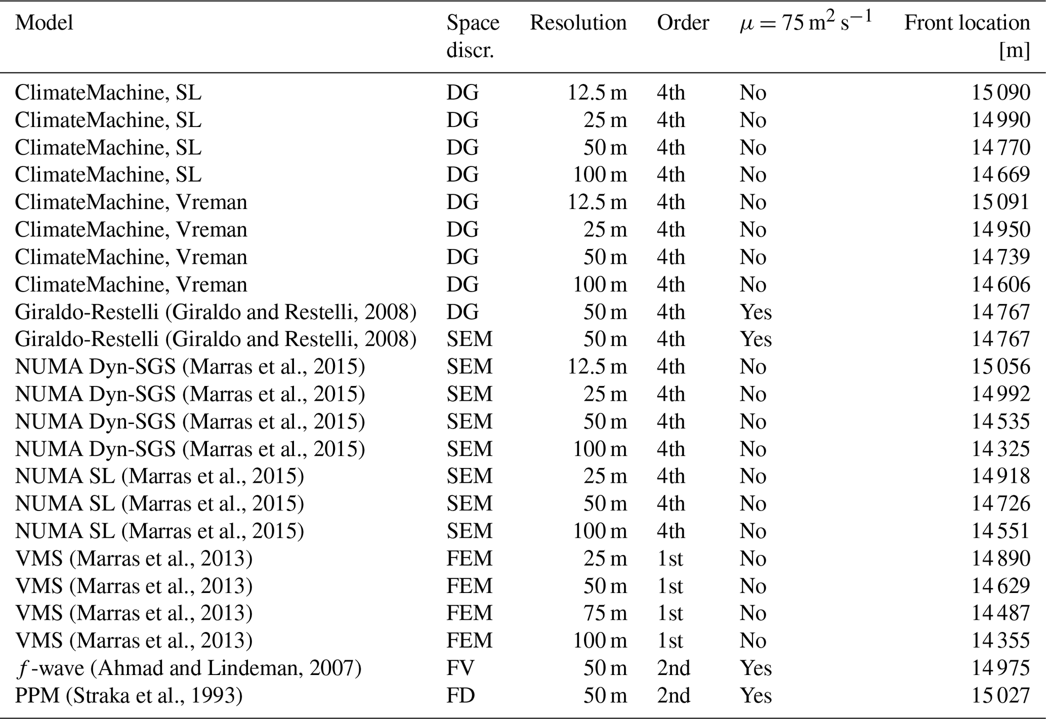
To reach solution grid convergence, this test is classically executed with a constant kinematic viscosity ν=75 m2 s−1. Increasingly finer structures are resolved when the resolution increases (Marras et al., 2012, 2015). A measure of solution fidelity is the front position, which we compare against other models in Appendix D for different resolutions. The ClimateMachine results show quantitative agreement with respect to the frontal location from a range of models with varying spatial discretizations at resolutions ranging from 12.5 to 100 m. This demonstrates the scope for capturing small-scale flow features with the numerics described in Sect. 3.
The structure of potential temperature at the final time t=900 s is shown in Fig. 4 for the Vreman and SL solutions. When Rusanov is the chosen numerical flux (Fig. 4a and b), the solutions are very similar although Vreman is visibly less dissipative for a prescribed value of the Smagorinsky coefficient Cs=0.18, with finer scales of motion apparent in the contours of potential temperature. Further quantitative analysis of the dissipative properties of the SGS models is reported in Sect. 5.6. Despite Vreman being less dissipative than SL, the Roe (Fig. 4c) and HLLC (Fig. 4d) fluxes contribute to additional numerical diffusion when compared to Rusanov fluxes. Detailed analysis of the interaction between numerical fluxes and subgrid-scale models will be presented in future articles.
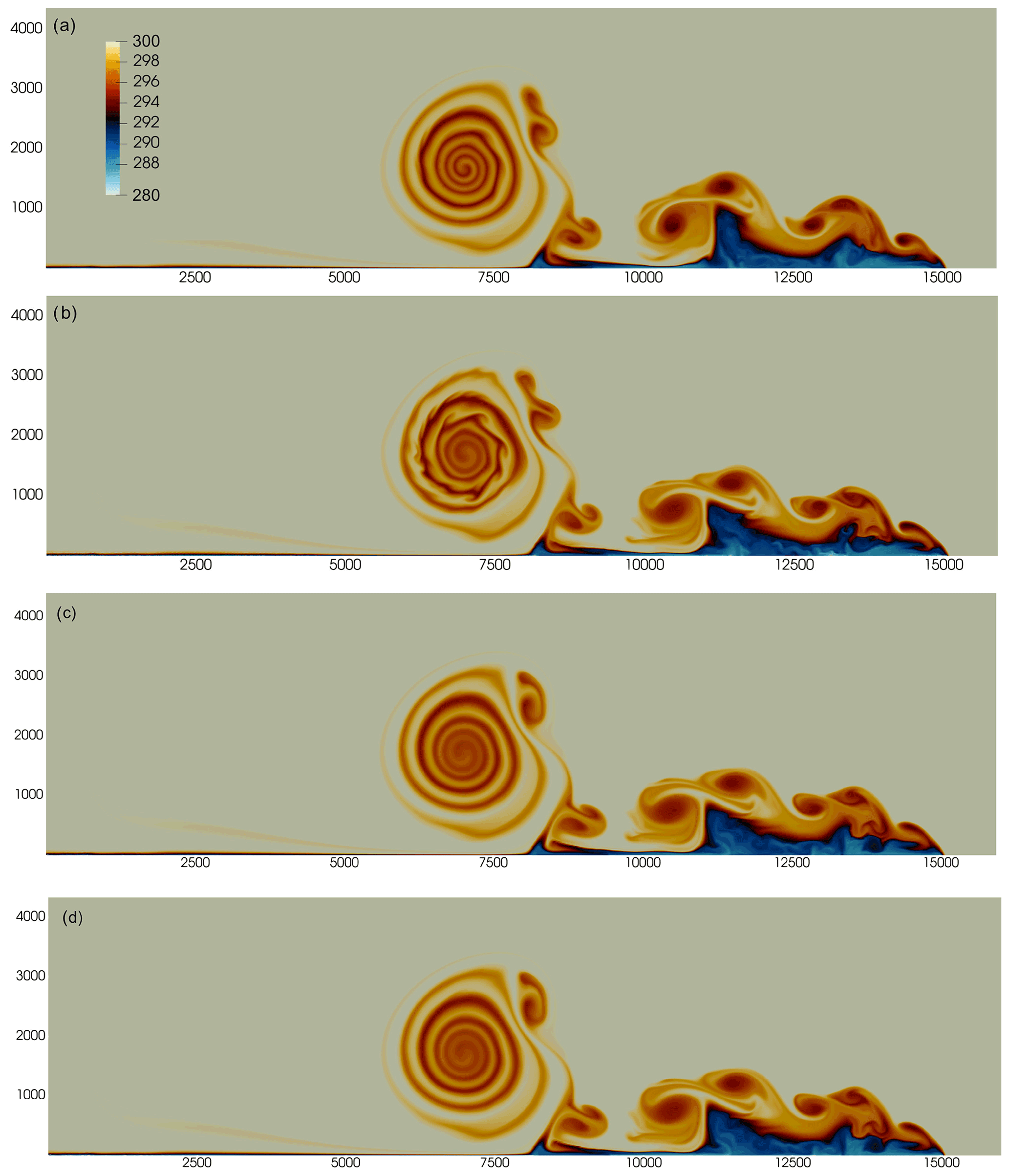
Figure 42.5D density current. Potential temperature θ (K) at t=900 s computed with an effective DG resolution of m with domain extents shown in meters. (a) Rusanov numerical flux with SL SGS. (b) Rusanov numerical flux with Vreman SGS. (c) Roe numerical flux with Vreman SGS. (d) HLLC numerical flux with Vreman SGS. The color scale ranges from θ=285 to 300 K. A shared color bar for all plots is shown in panel (a) for clarity.
5.4 Passive transport over warped grids
To verify the correct behavior of the DG implementation in the presence of topographic features, the simple passive advection test described by Schär et al. (2002) is used. The conservation law for the diffusive transport of a passive tracer χ is
which is approximated via DG in the same way as Eq. (16). For a scalar tracer variable χ, we model diffusive fluxes dχ such that
where δχ relates the ratio of turbulent diffusivity of the tracer to that of the energy and moisture variables. For this test case, however, tracer diffusivity is set to zero to assess the stability and transport properties when using a warped grid. The volume grid in ClimateMachine is built by stacking elements above the surface and warping them around the terrain profile. To reduce the element distortion across the domain, a linear grid damping function is used such that a topography-conforming surface of nodal points near the domain's bottom surface decays to a horizontal plane at higher altitudes (Gal-Chen and Somerville, 1975).
The initial scalar field χ is described by an elliptical perturbation centered on km with radii km such that
where χ0=1 and in the domain m3. An effective uniform grid resolution m is used for this test. The initial velocity profile is given by
where u0=10 m s−1, z1=4 km, and z2=5 km.
The topography is defined by the function
where h0=3 km, a=25 km, λ=8 km, and x0=75 km.
The contours of χ in Fig. 5 show minimal distortion in spite of the warped elements directly above the topographical feature, indicating that the DG transformation metrics from physical to logical space in the presence of topography do not adversely affect the solution. Deviation from the initial profile of tracer magnitudes is between −4 % and +2 % when the tracer is above the topographical feature, with maximum deviation amplitudes of −5 % and +3 % at the end of the test, showing a favorable comparison with the hybrid and SLEVE coordinate results presented in Schär et al. (2002).
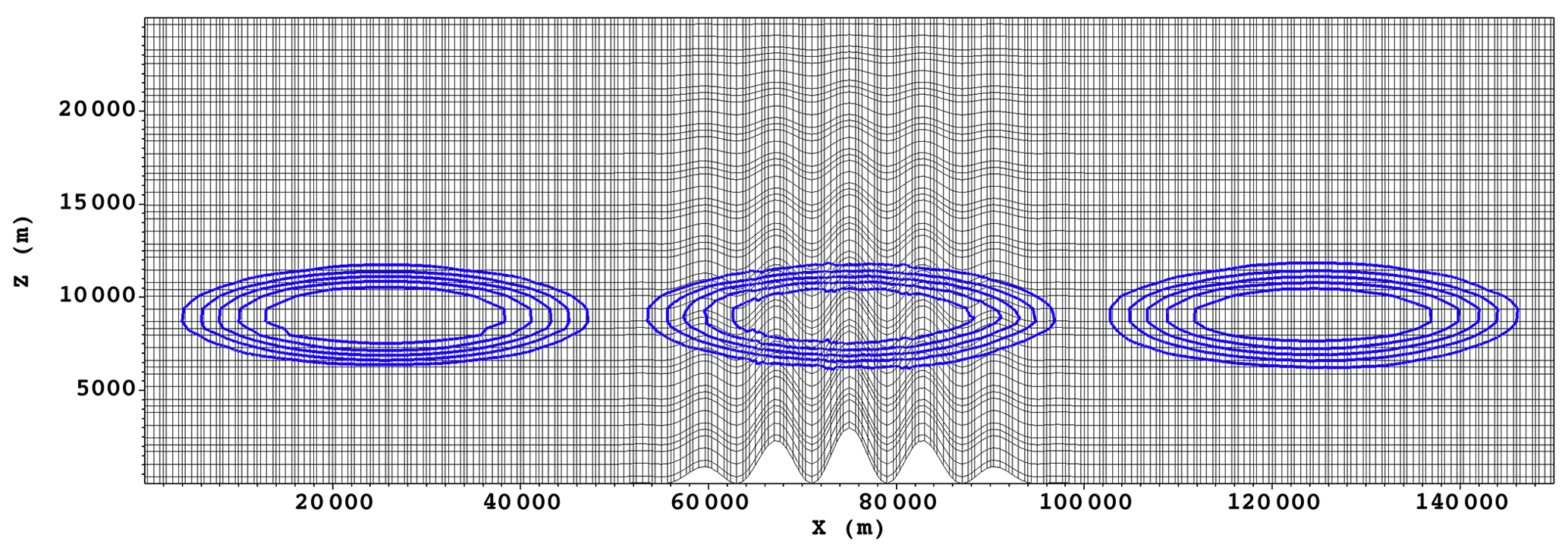
Figure 5Solution of the passive transport of scalar χ at three different time instances, with contours of tracer quantity χ (from 0, outermost contour, to 1, innermost contour) overlaid on a representation of nodal points on the underlying mesh. Tracer advection is driven by a prescribed velocity profile from left to right. As it crosses the deformed grid above the mountain ridge, only a minimal distortion of tracer contours is observed, which is completely recovered back to a smooth solution downwind of the ridge.
5.5 Mountain-triggered gravity waves
To assess the correct implementation of a Rayleigh sponge layer to attenuate fast, upward-propagating gravity waves before they reach the top of the domain, two steady-state mountain-triggered gravity wave problems suggested by Smith (1980) are solved. The sponge layer is described in Appendix A2. These problems consist of a flow that moves eastward with uniform horizontal velocity m s−1 in a doubly periodic domain. The flow impinges against a mountain of height hm and base length a centered at xc as
The background state is in hydrostatic balance with Brunt–Väisälä frequency 𝒩 such that
for a given surface potential temperature θsfc=Tsfc. The hydrostatically balanced pressure is
which yields, by means of the ideal gas law, the background density:
These tests are affected by spurious oscillations that appear approximately 5000 s into the simulation. In the absence of shear, because of the free-slip bottom and top boundaries, the SGS models are unable to introduce sufficient diffusion to remove the Gibbs modes so that an exponential filter (Hesthaven and Warburton, 2008b) of order 64 was applied on the velocity field to remove spurious modes. The filter assumes the form of
where s is the filter order, η is a function of the polynomial order, and is a parameter that controls the smallest value of the filter function for machine precision εM. In double precision, α≈36. The filter in this form is applied to perturbations of the prognostic variables from the balanced background state.
5.5.1 Linear hydrostatic
The linear hydrostatic case proposed by Smith (1979) consists of a neutrally stratified isothermal atmosphere with K. The background atmosphere is isothermal with temperature T0, resulting in a Brunt–Väisälä frequency of
The flow moves in a periodic channel along the x direction with velocity over a mountain with hm=1 m and a=10 000 m. A Rayleigh absorbing layer is added at zs=25 km with relaxation coefficient α=0.5 s−1, power γ=2, and domain top ztop=30 km (see Appendix A2 for details). The domain extends from 0 to 240 km in the horizontal direction. The steady-state solution at t=15 000 s is shown in Fig. 6a. It is consistent with the DG results shown by Giraldo and Restelli (2008).
5.5.2 Linear nonhydrostatic
The linear nonhydrostatic mountain waves are forced by a flow of uniform horizontal velocity over a mountain with hm=1 m and a=1000 m. The domain extends from 0 to 144 km in the horizontal direction and is 30 km high.
The steady-state solution at t=18 000 s is shown in Fig. 6b. It is consistent with results shown by Giraldo and Restelli (2008).
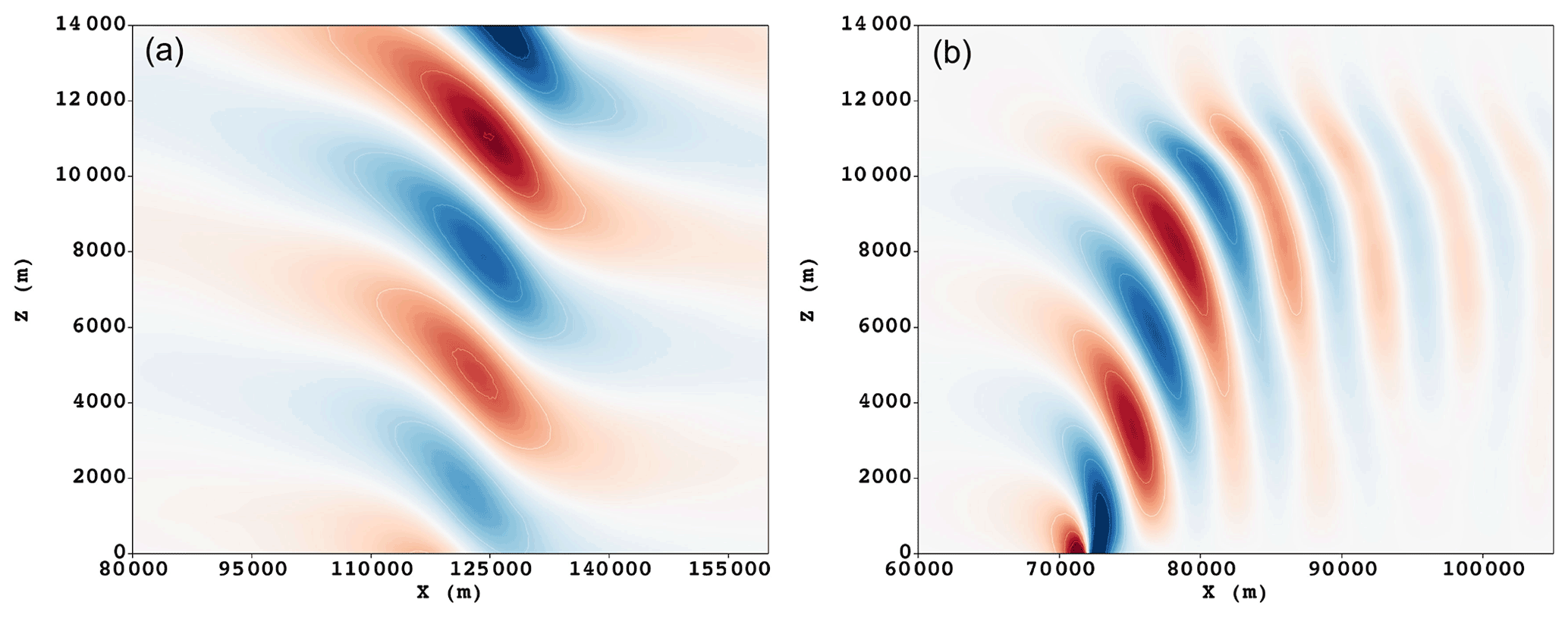
Figure 6Vertical velocity w for two linear mountain wave tests. Velocity contours are shown in the range from m s−1 (blue) to m s−1 (red). (a) Hydrostatic test at t=15 000 s, with an effective horizontal resolution Δx=500 m and effective vertical resolution Δz=240 m with N=4. (b) Nonhydrostatic test at t=18 000 s, with an effective horizontal resolution Δx=200 m and effective vertical resolution Δz=160 m with N=4.
5.6 Decaying Taylor–Green vortex
The decaying Taylor–Green vortex (TGV) is a classical test to estimate the dissipative properties of turbulence models in the absence of solid boundaries. The gravity-free flow is initialized in a triply periodic cube of dimensions . The solenoidal initial velocity field is defined as
with initial pressure
where k is the wavenumber, U0=100 m s−1, ρ0=1.178 kg m−3, and p∞=101 325 Pa. Fourth-order polynomials are used for all simulations considered in this section.
We first consider the volume-averaged kinetic energy, which provides insight into the dissipation characteristics of the flow with respect to nondimensionalized time . In integral form, the kinetic energy can be written as
where 〈⋅〉 denotes a volumetric average over the volume Ωh. If the flow is inviscid, the kinetic energy should be conserved. This is only valid if the numerics or SGS models do not introduce numerical dissipation or if all flow scales are well resolved. As such, the time series of kinetic energy is a metric that shows the point along the simulation at which the solution becomes under-resolved. The kinetic energy dissipation rate is the second quantity of interest, which allows us to quantify the rate of decay of kinetic energy over time. This is defined as
A third quantity of interest for this analysis is enstrophy, which is defined as the square of the vorticity norm:
The enstrophy of a fully resolved flow should go to infinity if the flow is inviscid. Therefore, enstrophy can be used as a criterion to estimate the effect of numerical dissipation.
By means of a three-dimensional fast Fourier transform (FFT) of the velocity field, the kinetic energy spectrum is calculated as
where , L is the characteristic length, A is a three-dimensional array of Fourier mode amplitudes, , , and . The TGV flow is simulated using both the SL and Vreman models on grids with 323, 643, 1283, and 1923 points. Figure 7 shows a 3D visualization of the flow at two different nondimensional times using zero Q-criterion isosurfaces, which identify balance between rotation and shear in the flow (Hunt et al., 1988). As the flow evolves, the flow generates smaller and smaller-scale vortices. Eventually, the flow becomes under-resolved, making it impossible to conserve kinetic energy. As the flow continues to evolve, an instability occurs, which causes the disintegration of the vortex sheet. After this point, the TGV's dynamics are controlled by the interaction of small-scale vortical structures formed by vortex stretching.
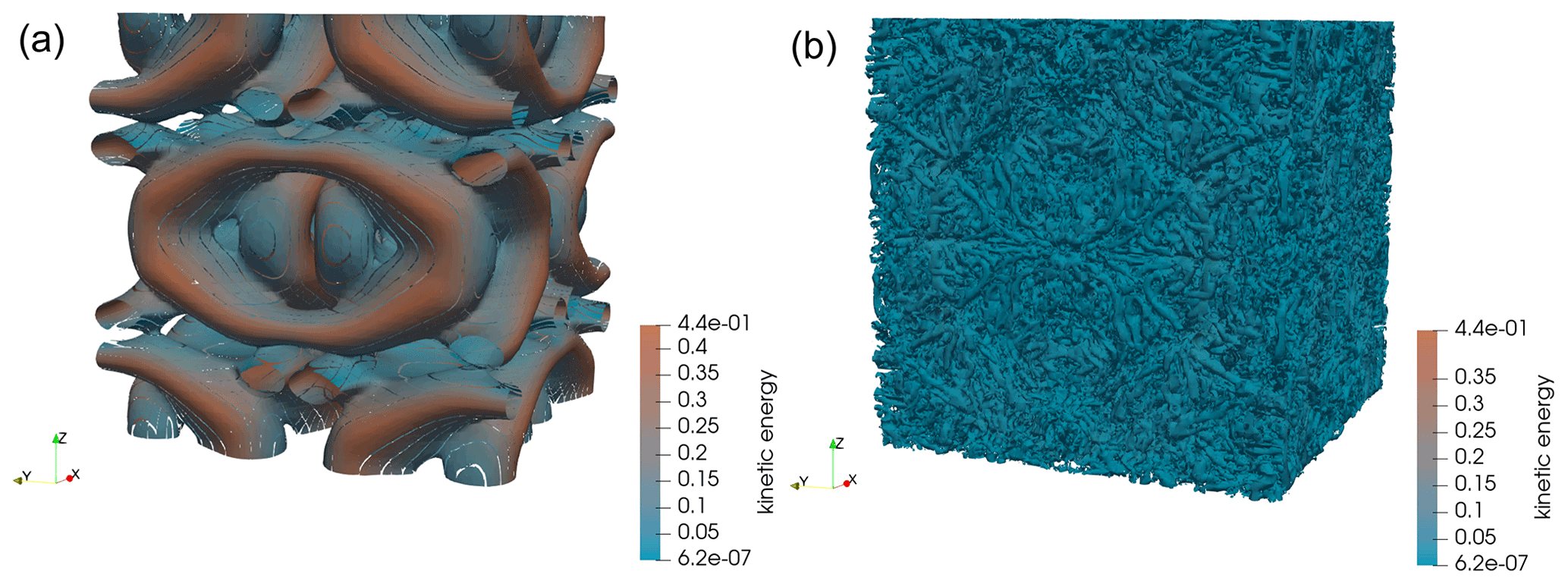
Figure 7Taylor–Green vortex. Isosurfaces of zero Q-criterion (these identify surfaces where the vorticity norm is identical to the strain rate magnitude) on a 1923 grid, corresponding to 48 elements of order 4 at (a) and (b) . Plots are shown for the Vreman solution. The isosurfaces of the Q-criterion are colored by dimensionless kinetic energy.
Results for the coarse-resolution simulations are presented in Fig. 8, and those for the fine-resolution simulations are shown in Fig. 9. Figure 8a shows that the kinetic energy changes with time for the 323 resolution simulations are distinctly different from their higher-resolution counterparts in Fig. 9a. The severe under-resolution of the flow seems to generate much larger amounts of dissipation early on. This is further demonstrated when comparing Figs. 8b and 9b. Beyond 643 resolution, the peaks in dissipation are larger as the resolution increases, since smaller vortices can be resolved before the instability eventually happens. The 323 simulations (Fig. 8b) have larger peaks than even the 1923 (Fig. 9b) simulations, demonstrating that the under-resolution of the vortex structures leads to different, more dissipative early-flow behavior.
Figure 9b shows that the 1283 and 1923 simulations using both SGS closures are characterized by a peak in the kinetic energy dissipation at . Brachet et al. (1983) and Brachet (1991) demonstrate this result for their direct numerical simulations (DNSs) of the Taylor–Green vortex for a Reynolds number . Examining Fig. 8b, the 643 simulations suggest a dissipation peak time of , and the 323 simulations suggest a dissipation peak time of . The underprediction of the time at which the peak occurs is due to an inability to resolve the vortices that appear early on in the flow's evolution at extremely coarse resolutions. This leads to the early appearance of the instability which causes the dissipation peak. Furthermore, we see that the kinetic energy decay occurs sooner for the lower-resolution simulations as a result of increased dissipation from the SGS models.
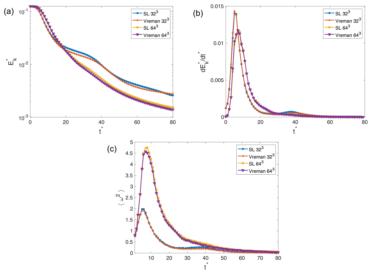
Figure 8Evolution of volumetrically averaged (a) kinetic energy represented on a semi-logarithmic scale, (b) kinetic energy dissipation, and (c) enstrophy, each computed on 323 and 643 grids with the Vreman and SL SGS models.
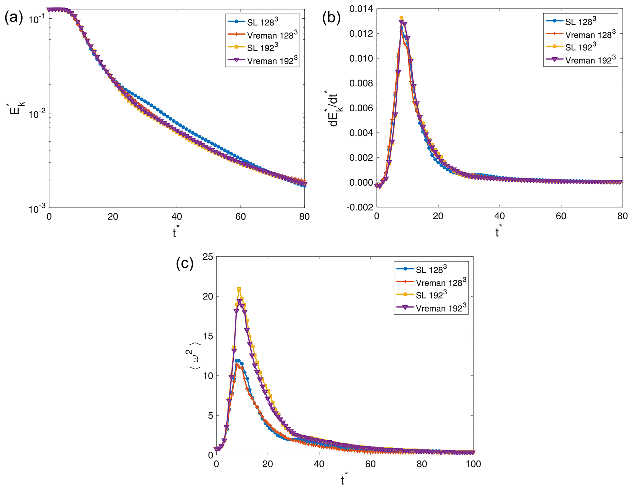
Figure 9Evolution of volumetrically averaged quantities in the numerical solution to the Taylor–Green vortex problem computed on 1283 and 1923 grids with the Vreman and SL SGS models.
Figure 9c also shows that the flow's enstrophy behaves as expected, with peak values at coinciding with peaks in kinetic energy. The higher-resolution simulations are able to reach a higher enstrophy than the lower-resolution simulations as they are naturally able to resolve more vortical motion. On the other hand, the choice of SL or Vreman models seems to have very little impact on the ability to resolve more small-scale eddies for low resolutions. However, the SL SGS scheme leads to higher enstrophy than the Vreman SGS scheme, increasingly so as resolution increases.
Figure 10 shows the kinetic energy spectra obtained for the higher-resolution simulations used for this test. All simulations present peaks in their respective spectra at k=2 to 4, which persist even as the flow evolves over time. These peaks are explained by Drikakis et al. (2007) as being imprinted on the spectra by the initial velocity field. Furthermore, as the flow evolves, all spectra show a slope close to the theoretical of homogeneous turbulence and eventually decay towards a k−3 slope at higher wavenumbers. This behavior is consistent with the DNS results of Brachet et al. (1983), who showed, using DNS, that this transition occurs around k=60.
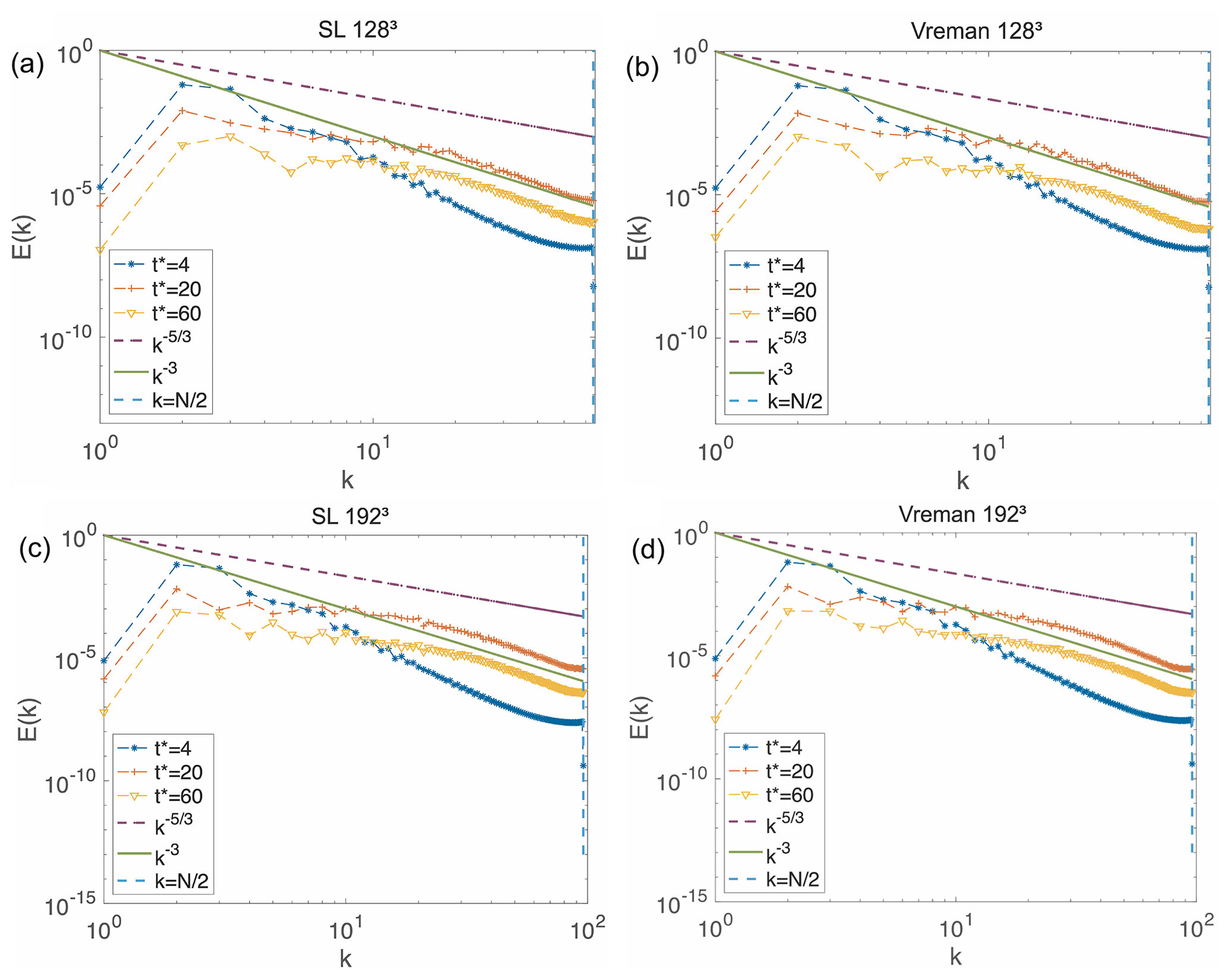
Figure 10Kinetic energy spectra obtained using (a) 1283 points and SL, (b) 1283 points and Vreman, (c) 1923 points and SL, and (d) 1923 points and Vreman.
5.7 Barbados Oceanographic and Meteorological Experiment (BOMEX)
BOMEX features a shallow-cumulus-topped boundary layer as described in Holland and Rasmusson (1973). The setup of this test follows Siebesma et al. (2003). The initial profiles are characterized by a well-mixed sub-cloud layer below 500 m, a cumulus layer between 500 and 1500 m, an inversion layer up to 2000 m, and a free troposphere above. Large-scale forcing includes prescribed large-scale subsidence, horizontal advective drying, radiative cooling, and pressure gradient effects. Sensible and latent heat fluxes at the surface are prescribed to W m−2 and W m−2. Additional detail on the application of boundary conditions is presented in Appendix A. The domain, m3, is doubly periodic in the x and y directions. A Rayleigh sponge layer (see Appendix A2 for details) is applied along the z direction to damp upward-propagating gravity waves. On the bottom surface, a momentum drag forcing is applied (see Appendix A1). The effective horizontal and vertical resolutions are m and Δz=40 m, respectively. The simulation time is 6 h.
Figure 11 shows the vertical profiles of the domain mean thermodynamic and turbulence properties over the last hour of the simulations. Figure 12 shows the time series of liquid water paths (LWPs), cloud cover, and turbulence kinetic energy. The time-averaged results of the vertical profiles of θl,ql, cloud fraction, and during the last hour are in good agreement with the same quantities presented by Siebesma et al. (2003). The SGS model does not have much effect on the simulation characteristics, except that the Vreman SGS model produces a stronger peak in the variance of vertical velocity, , near the cloud top. Although the difference is mild, it is possibly due to the low dissipation nature of the Vreman's model. Excluding the first hour of flow spin-up, the results compare well with PyCLES (Pressel et al., 2015) and fall within the ensemble range shown in Fig. 2 of Siebesma et al. (2003). PyCLES solves the anelastic conservation equations with entropy as the prognostic thermodynamic variable using weighted essentially non-oscillatory (WENO) numerics. Differences in the initial conditions (as seen in the initial LWP in Fig. 12) are likely contributing to the initial mismatch in horizontally averaged properties of moisture and turbulence. Details on the computation of horizontally averaged profiles can be found in Appendix B.
A large-domain simulation of BOMEX with effective horizontal resolution m and vertical resolution Δz=20 m in a km3 domain was executed using 16 GPUs on the Google Cloud Platform. The simulation was executed using 1D IMEX time integration (1D implicit in the vertical direction and 2D explicit in the horizontal direction) at maximum horizontal advective Courant number C=0.9. A visualization of instantaneous shallow cumulus structures is shown in Fig. 13.
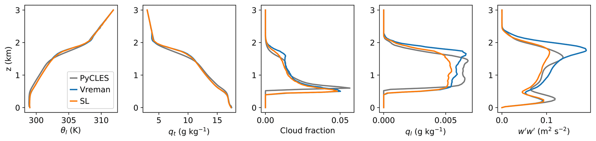
Figure 11BOMEX. Profile of the mean state of liquid potential temperature, total specific humidity, cloud fraction, liquid water specific humidity, and variance of the vertical velocity fluctuations averaged along the last hour of the simulation. The solutions with PyCLES and ClimateMachine were calculated with effective grid resolution m and Δz=40 m. Results calculated with Vreman (blue lines) and SL SGS (orange lines) models in ClimateMachine are compared against results of PyCLES (grey lines) in its paired SGS modality using the SL model.
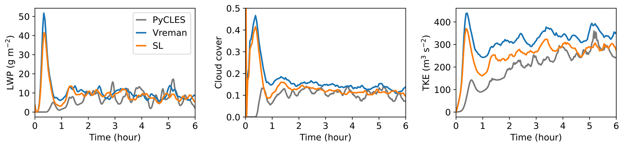
Figure 12BOMEX. From left to right, time series of horizontally averaged LWP, cloud cover, and turbulence kinetic energy diagnosed from ClimateMachine using Vreman and SL. These results are consistent with ensemble results presented in Fig. 2 of the intercomparison study by Siebesma et al. (2003). Line colors are as in Fig. 11.
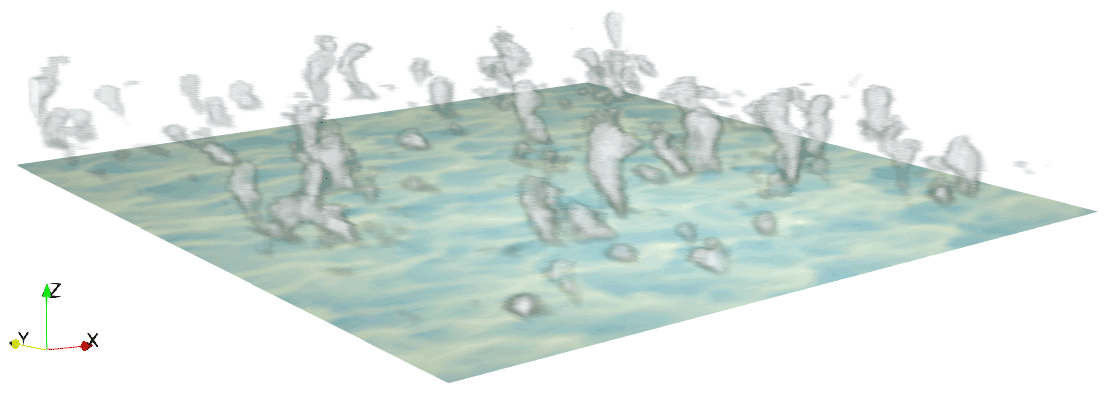
Figure 13BOMEX. Instantaneous visualization of the shallow cumulus structures on a km domain. The white shading of the volume rendering of the cloud corresponds to a maximum value of kg kg−1; a maximum kg kg−1 is shown on the bottom surface in light yellow shading. The simulation was executed using 16 GPUs on the Google Cloud Platform.
We respectively define the time-dependent normalized total mass and energy changes as
and
where t0 indicates the initial time and Ω is the full domain. Figure 14 shows ΔM(t) and Δρetot(t) for a 1 h simulation of a moist rising thermal bubble. The SL eddy viscosity model was used to represent under-resolved diffusive fluxes. This simulation was run using free-slip boundary conditions with adiabatic walls. We note that the loss of energy and mass in the system is contained to 𝒪(10−15): that is, numerical roundoff error. This result highlights a key benefit of the general formulation of the prognostic conservation equations in flux form, which guarantees conservation properties up to source or sink contributions.
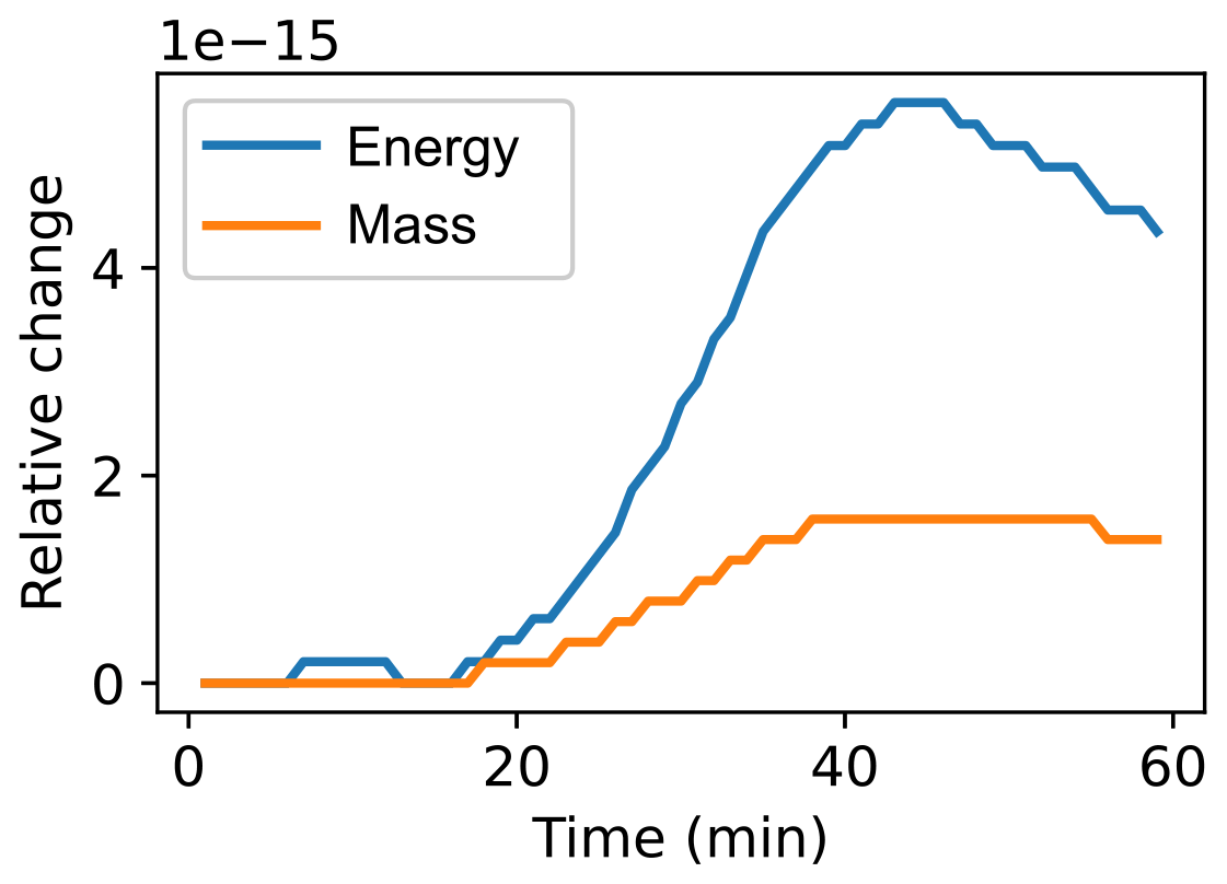
Figure 14Time evolution of the mass and total energy loss (relative change when compared against initial conditions) for a moist thermal bubble simulation. Blue line: relative change in energy; orange line: relative change in mass.
Demonstration of favorable scaling capabilities across multiple hardware types is critical to the utility of ClimateMachine as a competitive tool for large-eddy simulations. Toward this, we first examine strong scaling on CPU architectures. The rising thermal bubble problem described in Sect. 5.2 is used as the test problem, with its domain extents modified to form an 8.192 km3 cube, with an effective nodal resolution of 32 m to ensure that CPU memory on a single rank is maximally loaded. For tests with multiple MPI ranks, each rank resides on a unique node to ensure communication overhead is appropriately represented; in practice, one would expect to use multiple ranks per node. Scaling across multiple threads is not assessed in the present work. Figure 15 shows the speed-up in time to solution for 10 time integration steps of the test problem with for both dry and moist simulations. We exclude checkpoint, diagnostic, and periodic runtime output steps from time-to-solution measurements. In both dry and moist simulations, we see a speed-up of approximately 19.7 when using 32 ranks compared with the corresponding single-rank simulation.
A single-rank GPU run of the test problem on a 6.144 km3 domain with 32 m effective resolution (restricted by GPU memory capacity) has a wall-clock time for 10 integration steps of 314 s. The wall-clock time for a 32-rank CPU run was 449 s for a problem 2.37 times larger.
This provides an estimate for a comparison between CPU and GPU hardware performance. However, the balance between memory bandwidth limits and computing operation limits guides the maximum scaling possible on the GPU hardware relative to its CPU counterpart, so this cannot be interpreted as a direct comparison across hardware types. Based on the present results, we conclude that it is more feasible to pursue strong scaling improvements on CPU hardware than on GPU hardware. Further optimization and exploration of scaling in ClimateMachine are ongoing work. Additional details on the hardware used for scaling tests can be found in Appendix C.
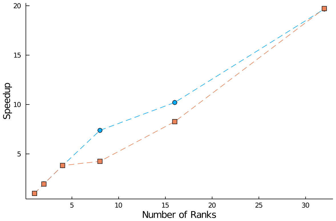
Figure 15Speed-up of the time integration (solver) step relative to the time to solution for a single-rank simulation of the rising thermal bubble problem in an 8.192 km3 domain with a uniform effective resolution of 32 m (with fourth-order polynomials). Blue circles: dry simulation; orange squares: moist simulation.
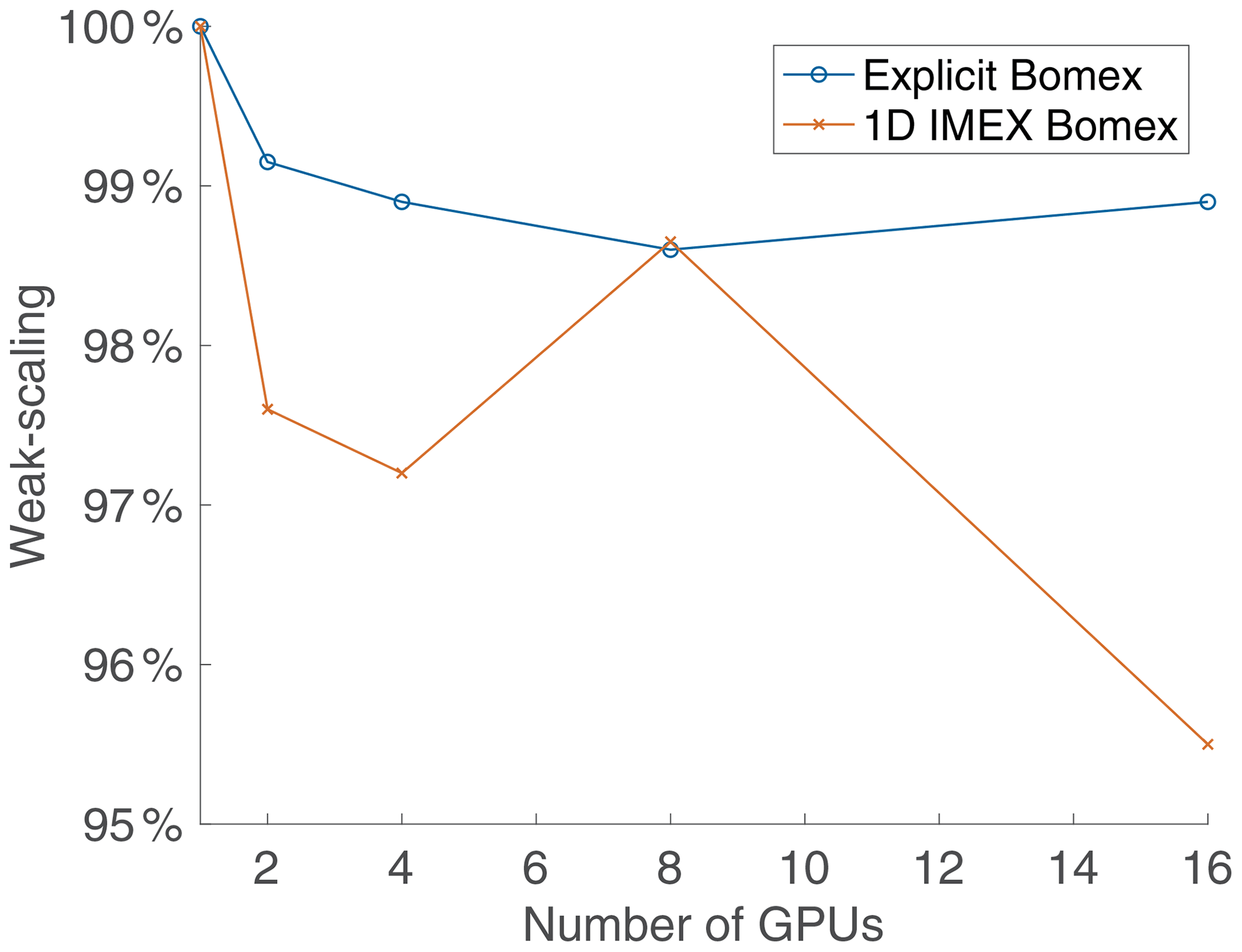
To test the multi-GPU scalability of ClimateMachine, we first execute a BOMEX setup that is sufficiently large to saturate one GPU. The single-GPU execution represents the baseline from which we calculate the average time per time step denoted by t1. We then expand the domain size to match an increase in the number of GPUs and measure the average time per time step. Our scaling is then obtained as the ratio , with tn being the average time per time step obtained with n GPUs. The results are obtained using up to 16 NVIDIA Tesla V100 GPUs running Julia version 1.4.2, CUDA 10.0, and CUDA-aware OpenMPI 4.0.3. Figure 16 shows excellent weak scaling for up to 16 GPUs on Google Cloud Platform resources. Over 95 % weak scaling was achieved with 1D IMEX time integration and over 98 % for the simulation with explicit time stepping. This is an encouraging result and supports the ability to prototype smaller problem setups and deploy larger simulations in the ClimateMachine limited-area configuration at identical resolutions without significantly compromising the time to solution.
This paper introduced and assessed the LES configuration of ClimateMachine, a new Julia-language simulation framework designed for parallel CPU and GPU architectures. Notable features of this LES framework are the following:
-
conservative flux form model equations for mass, momentum, total energy, and total moisture to ensure global conservation of dynamical variables of interest (up to nonconservative source or sink processes);
-
discontinuous Galerkin discretization with element-wise evaluation of the approximations to volume and interface integrals, resulting in reduced time to solution due to MPI operations;
-
application of model equations to the solution of benchmark problems in typical LES codes, including atmospheric flows in the shallow cumulus regime (BOMEX); and
-
demonstration of strong scaling on CPUs with up to 32 MPI ranks (speed-up of 19.7 in time to solution) and weak scaling with up to 16 GPUs (95 %–98 %) in both dry and moist simulation configurations.
A1 Solid walls and wall fluxes
A1.1 Momentum
Rigid surfaces are considered impenetrable such that the wall-normal component of the velocity vanishes at rigid boundaries by imposing . The viscous sublayer is not explicitly resolved, and a momentum sink is applied to model the effect of wall-shear stresses. While the wall-normal advective momentum flux vanishes, the wall-normal viscous or SGS momentum flux, also known as the bulk surface stress (units of Pa),
is not necessarily negligible. Here, is the strain rate tensor of the near-surface wall-parallel velocity, up. We note that, throughout Appendix A, n refers to the inward-pointing normal vector at domain boundaries, distinct from the prior definition of the element-interface normal vector in Sect. 3.
In the case of free-slip conditions at a solid surface (indicated by subscript “sfc”), there is no viscous or SGS momentum transfer between the atmosphere and the surface, such that
Because the momentum flux tensor depends linearly on velocity derivatives, this amounts to homogeneous Neumann boundary conditions on velocity components parallel to the surface. On the other hand, viscous drag is imposed by the classical aerodynamic drag law,
where the quantities with subscript int are evaluated at an interior point xint adjacent to the surface. The drag coefficient,
can depend parametrically on state variables Y(x,t) and on the position xint of the interior point relative to the surface. In the present implementation, the plane of interior points relevant to boundary flux evaluation is interpreted as the first layer of interior nodes in the surface-adjacent elements. The drag law boundary condition amounts to inhomogeneous Neumann boundary conditions on velocity components parallel to the surface.
A1.2 Specific humidity
As for momentum, the advective specific humidity fluxes normal to a rigid surface vanish, but the diffusive or SGS specific humidity fluxes normal to the surface may not vanish. Normal components of SGS fluxes of condensate, ql, are generally set to zero at boundaries,
implying homogeneous Neumann boundary conditions () on the condensate specific humidities. The total SGS specific humidity flux then reduces to the vapor flux at the surface. SGS turbulent deposition of condensate (fog) on the surface can in principle occur; representing this would require nonzero condensate fluxes at the surface. With the assumption of zero condensate boundary fluxes, we have
where evaporation (measured in kg m−2 s−1), or condensation if negative, is given by
Evaporation can be zero (water impermeable) or it can be given as a function of Y at the surface according to
which, numerically, translates into an inhomogeneous Neumann boundary condition on the vapor specific humidity.
A1.3 Energy
As for momentum and humidity, the advective energy fluxes normal to a rigid surface vanish, but the diffusive or SGS flux of total enthalpy, htot, normal to the surface (units of W m−2),
may not vanish. Because the kinetic energy contribution to the total enthalpy flux near a surface is usually 3–4 orders of magnitude smaller than the thermal and potential energy components, it is generally neglected so that the total enthalpy flux J+D reduces to a flux of moist static energy . The surface can be insulating, in which case the SGS transfer of total enthalpy between the atmosphere and the surface is zero:
which, from a numerical point of view, translates to a homogeneous Neumann condition on the total enthalpy () or, by neglecting kinetic energy, on MSE such that (). With known MSE, the moist static energy flux (MSEF) at the surface is given by
with Ch,int the thermal exchange coefficient.
The value of can also be assigned by the summation of given LHF and SHF, as done in the case of BOMEX described in Sect. 5.
A2 Non-reflecting top boundary
To prevent the reflection of fast, upward-propagating gravity waves at the top boundary, a Rayleigh damping sponge is added to the right-hand side of the momentum equation (see Sect. 5). The damping in the momentum equations takes the form
where urelax is a specified background velocity to which the flow is relaxed within the absorbing layer, with a characteristic relaxation coefficient τs. Of the many alternative options known for τs (e.g., Durran and Klemp, 1983), the default in ClimateMachine is
where the absorbing sponge layer starts at z=zs, γ is a positive even power typically set to 2, and α>0 is a relaxation coefficient typically of order 𝒪(1 s−1).
A3 Numerical implementation
For the boundary velocity corresponding to the impenetrable wall condition, we use the following reflecting condition:
The no-slip condition follows from Eq. (A12) by setting all components of ubc=0. Boundary conditions on a scalar χ are similarly specified as follows:
Nonzero mass flux boundary conditions can be imposed at penetrable or free surfaces by applying the transmissive boundary condition:
Diffusive fluxes are applied by a direct specification of the wall-normal fluxes, and over-specified boundary conditions are avoided by using only the interior (−) gradients and first-order fluxes.
Since the flow is compressible, we use density-weighted Favre averages following Canuto (1997) when computing horizontally averaged statistics. For a scalar ϕ, the density-weighted average at a given height level z is defined by
where 〈⋅〉 denotes a horizontal mean. All calculations of horizontal statistics are done on the DG nodal mesh to avoid introducing interpolation errors (Yamaguchi and Feingold, 2012), with metric terms accounted for in the descriptions of diagnostic variables. The density-weighted vertical eddy flux for a variable ϕ is defined by
where
denotes the deviation from the density-weighted mean. The variance can then be defined as
This section summarizes the hardware characteristics for the primary computing resources used in tests throughout this paper. This is particularly relevant to the data presented in Sect. 7. Compute nodes for the CPU tests were 14-core Intel Xeon (2.4 GHz), with a maximum memory capacity of 1.5 TB. GPU nodes on this cluster were of 14-core Intel Broadwell (2.4 GHz) type with 28 cores per node and 256 GB of memory per node. Compute nodes on the Google Cloud Platform leverage Tesla V100 GPUs available for general-purpose use.
This section provides additional information on the comparison of the density current benchmark in ClimateMachine with existing literature references in Table D1.
(Giraldo and Restelli, 2008)(Giraldo and Restelli, 2008)(Marras et al., 2015)(Marras et al., 2015)(Marras et al., 2015)(Marras et al., 2015)(Marras et al., 2015)(Marras et al., 2015)(Marras et al., 2015)(Marras et al., 2013)(Marras et al., 2013)(Marras et al., 2013)(Marras et al., 2013)(Ahmad and Lindeman, 2007)(Straka et al., 1993)Table D1Summary of frontal locations for the density current test case from existing literature. Results tabulated are of the front location at t=900 s. The results are reported for the following models: ClimateMachine with SL and Vreman, finite-element model (FEM) variational multiscale stabilization (VMS), f-wave, filtered spectral elements (SEs), filtered discontinuous Galerkin (DG), and the piecewise parabolic method (PPM). NUMA is the Nonhydrostatic Unified Model of the Atmosphere.
ClimateMachine is an open-source framework that is maintained on GitHub: https://github.com/CliMA/ClimateMachine.jl (last access: 20 June 2022). Documentation for installing and running ClimateMachine is available at https://clima.github.io/ClimateMachine.jl/latest/ (last access: 20 June 2022). The version used in this paper is v0.2.0, which can be downloaded from https://doi.org/10.5281/zenodo.5542395 (Climate Modeling Alliance, 2020) or https://github.com/CliMA/ClimateMachine.jl/releases/tag/v0.2.0 (last access: 20 June 2022). The parameters included in Table 1 are available in the accompanying CLIMAParameters.jl Julia package. The code is released under the Apache License, version 2.0
The test cases presented in the paper are available in the following directory locations in the source code.
-
Sect. 5.1: /test/Numerics/DGMethods/Euler/isentropicvortex.jl
-
Sect. 5.2: /tutorials/Atmos/risingbubble.jl
-
Sect. 5.3: /tutorials/Atmos/densitycurrent.jl
-
Sect. 5.4: /experiments/AtmosLES/schar_scalar_advection.jl
-
Sect. 5.5: /experiments/AtmosLES/agnesi_hs_lin.jl and /experiments/AtmosLES/agnesi_nh_lin.jl
-
Sect. 5.6: /experiments/AtmosLES/taylor_green.jl
-
Sect. 5.7: /experiments/AtmosLES/bomex_model.jl and /experiments/AtmosLES/bomex_les.jl
Configuration instructions and methods for resolution, numerical flux schemes, boundary conditions, and turbulence model specification can be found in the code documentation at https://clima.github.io/ClimateMachine.jl/v0.2/ (Climate Modeling Alliance, 2020). Instructions for installing and launching simulations can be accessed at https://clima.github.io/ClimateMachine.jl/v0.2/GettingStarted/RunningClimateMachine/ (last access: 20 June 2022).
AS contributed to analysis, methodology, software, and writing – review and editing. YT contributed to analysis, visualization, software, and writing – review and editing. SM contributed to conceptualization, methodology, software, and writing – original draft preparation, review, and editing. ZS contributed to software, analysis, visualization, and writing – review and editing. CK developed software. SB developed software. KP developed software and contributed to the analysis. MW was responsible for methodology and software. THG contributed to methodology, software, and writing – review and editing. JEK contributed to conceptualization, methodology, and software. VC developed software. LCW contributed to conceptualization, methodology, and software. FXG contributed to conceptualization, methodology, software, and writing – review and editing. TS contributed to conceptualization, methodology, software, project administration, and writing – original draft preparation, review, and editing.
At least one of the co-authors is a member of the editorial board of Geoscientific Model Development. The peer-review process was guided by an independent editor, and the authors have no other competing interests to declare.
Publisher's note: Copernicus Publications remains neutral with regard to jurisdictional claims in published maps and institutional affiliations.
The computations presented here were conducted at the Resnick High-Performance Computing Center, a facility supported by the Resnick Sustainability Institute at the California Institute of Technology (formerly known as the Central HPC Cluster, with partial support by a grant from the Gordon and Betty Moore Foundation), and on the Google Cloud Platform with in-kind support by Google. We thank the Google team for their assistance with operations on the Google Cloud Platform.
This research was made possible by the generosity of Eric and Wendy Schmidt by recommendation of the Schmidt Futures program and by the Paul G. Allen Family Foundation, Charles Trimble, the Audi Environmental Foundation, the Heising-Simons Foundation, and the National Science Foundation (grants AGS-1835860 and AGS-1835881). Additionally, Valentin Churavy was supported by the Defense Advanced Research Projects Agency (DARPA, agreement HR0011-20-9-0016) and by the NSF (grant OAC-1835443). Part of this research was carried out at the Jet Propulsion Laboratory, California Institute of Technology, under a contract with the National Aeronautics and Space Administration.
This paper was edited by Travis O'Brien and reviewed by two anonymous referees.
Abdi, D. S., Giraldo, F. X., Constantinescu, E., Lester III, C., Wilcox, L., and Warburton, T.: Acceleration of the Implicit-Explicit Non-Hydrostatic Unified Model of the Atmosphere (NUMA) on Manycore Processors, Int. J. High Perform. C., 33, 242–267, https://doi.org/10.1177/1094342017732395, 2017a. a
Abdi, D. S., Wilcox, L. C., Warburton, T. C., and Giraldo, F. X.: A GPU-accelerated continuous and discontinuous Galerkin non-hydrostatic atmospheric model, Int. J. High Perform. C., 33, 81–109, https://doi.org/10.1177/1094342017694427, 2017b. a, b, c, d, e
Ahmad, N. and Lindeman, J.: Euler solutions using flux-based wave decomposition, Int. J. Numer. Meth. Fl., 54, 47–72, https://doi.org/10.1002/fld.1392, 2007. a, b, c
Balaji, V.: Climbing down Charney's ladder: machine learning and the post-Dennard era of computational climate science, Philos. T. Roy. Soc. A, 379, 20200085, https://doi.org/10.1098/rsta.2020.0085, 2021. a
Bao, L., Klöfkorn, R., and Nair, R. D.: Horizontally Explicit and Vertically Implicit (HEVI) Time Discretization Scheme for a Discontinuous Galerkin Nonhydrostatic Model, Mon. Weather Rev., 143, 972–990, https://doi.org/10.1175/MWR-D-14-00083.1, 2015. a
Bassi, F. and Rebay, S.: A high-order discontinuous Galerkin finite element method solution of the 2d Euler equations, J. Comput. Phys., 138, 251–285, https://doi.org/10.1006/jcph.1997.5454, 1997. a, b
Bezanson, J., Edelman, A., Karpinski, S., and Shah, V. B.: Julia: A Fresh Approach to Numerical Computing, SIAM Rev., 59, 65–98, https://doi.org/10.1137/141000671, 2017. a
Bezanson, J., Chen, J., Chung, B., Karpinski, S., Shah, V. B., Vitek, J., and Zoubritzky, L.: Julia: Dynamism and Performance Reconciled by Design, Proc. ACM Program. Lang., 2, 1–23, https://doi.org/10.1145/3276490, 2018. a
Bott, A.: Theoretical considerations on the mass and energy consistent treatment of precipitation in cloudy atmospheres, Atmos. Res., 89, 252–269, 2008. a, b
Boyd, J. P.: The erfc-log filter and the asymptotics of the Euler and Vandeven sequence accelerations, edited by: Ilin, A. V. and Scott, L. R., Proceedings of the Third International Conference on Spectral and High Order Methods, Houston Journal of Mathematics, 267–276, 1996. a
Brachet, M. E.: Direct simulation of three-dimensional turbulence in the Taylor-Green vortex, Fluid Dyn. Res., 8, 1–8, https://doi.org/10.1016/0169-5983(91)90026-f, 1991. a
Brachet, M. E., Meiron, D. I., Orszag, A., Nickel, B. G., Morf, R. H., and Frisch, U.: Small-scale structure of the Taylor-Green vortex, J. Fluid Mech., 130, 411–452, https://doi.org/10.1017/S0022112083001159, 1983. a, b
Canuto, V. M.: Compressible turbulence, Astrophys. J., 482, 827–851, https://doi.org/10.1086/304175, 1997. a
Carpenter, M. H. and Kennedy, C. A.: Fourth-order 2N-storage Runge-Kutta schemes, Tech. Rep. NASA TM-109112, National Aeronautics and Space Administration, Langley Research Center, Hampton, VA, 1994. a
Chow, F. K. and Moin, P.: A further study of numerical errors in large-eddy simulations, J. Comput. Phys., 184, 366–380, https://doi.org/10.1016/S0021-9991(02)00020-7, 2003. a
Climate Modeling Alliance: ClimateMachine.jl (0.2.0), Zenodo [code], https://doi.org/10.5281/zenodo.5542395, 2020. a, b
Deardorff, J. W.: A numerical study of three-dimensional turbulent channel flow at large Reynolds numbers, J. Fluid Mech., 41, 452–480, https://doi.org/10.1017/S0022112070000691, 1970. a, b
Deardorff, J. W.: Three-dimensional numerical study of the height and mean structure of a heated planetary boundary layer, Bound. Lay. Meteorol., 7, 81–106, https://doi.org/10.1007/BF00224974, 1974. a
Deardorff, J. W.: Usefulness of liquid-water potential temperature in a shallow-cloud model, J. Appl. Meteorol., 15, 98–102, https://doi.org/10.1175/1520-0450(1976)015<0098:UOLWPT>2.0.CO;2, 1976. a
Deardorff, J. W.: Stratocumulus-capped mixed layers derived from a three-dimensional model, Bound. Lay. Meteorol., 18, 495–527, https://doi.org/10.1007/BF00119502, 1980. a, b, c
Deville, M. O., Fischer, P. F., and Mund, E. H.: High-order methods for incompressible fluid flow, Cambridge University Press, https://doi.org/10.1017/CBO9780511546792, 2002. a
Dipankar, A., Stevens, B., Heinze, R., Moseley, C., Zängl, G., Giorgetta, M., and Brdar, S.: Large eddy simulation using the general circulation model ICON, J. Adv. Model. Earth Sy., 7, 963–986, https://doi.org/10.1002/2015MS000431, 2015. a
Drikakis, D., Fureby, C., and Youngs, F.: Simulation of transition and turbulence decay in the Taylor–Green vortex, J. Turbulence, 8, 1–12, https://doi.org/10.1080/14685240701250289, 2007. a
Durran, D. and Klemp, J.: A compressible model for the simulation of moist mountain waves, Mon. Weather Rev., 111, 2341–2361, https://doi.org/10.1175/1520-0493(1983)111<2341:ACMFTS>2.0.CO;2, 1983. a
Toro, E. F., Spruce, M., and Speares, W.: Restoration of the Contact Surface in the HLL–Riemann Solver, Shock Waves, 4, 25–34, https://doi.org/10.1007/BF01414629, 1994. a
Fuhrer, O., Osuna, C., Lapillonne, X., Gysi, T., Cumming, B., Bianco, M., Arteaga, A., and Schulthess, T. C.: Towards a performance portable, architecture agnostic implementation strategy for weather and climate models, Supercomput. Front. Inn., 1, 45–62, https://doi.org/10.14529/jsfi140103, 2014. a
Fuhrer, O., Chadha, T., Hoefler, T., Kwasniewski, G., Lapillonne, X., Leutwyler, D., Lüthi, D., Osuna, C., Schär, C., Schulthess, T. C., and Vogt, H.: Near-global climate simulation at 1 km resolution: establishing a performance baseline on 4888 GPUs with COSMO 5.0, Geosci. Model Dev., 11, 1665–1681, https://doi.org/10.5194/gmd-11-1665-2018, 2018. a
Gal-Chen, T. and Somerville, R.: Numerical solution of the Navier-Stokes equations with topography, J. Comput. Phys., 17, 276–310, https://doi.org/10.1016/0021-9991(75)90054-6, 1975. a
Ghosal, S.: An Analysis of Numerical Errors in Large-Eddy Simulations of Turbulence, J. Comput. Phys., 125, 187–206, https://doi.org/10.1006/jcph.1996.0088, 1996. a
Giraldo, F. X.: An Introduction to Element-based Galerkin Methods on Tensor-Product Bases: Analysis, Algorithms, and Applications, Springer, https://doi.org/10.1007/978-3-030-55069-1, 2020. a
Giraldo, F. X. and Restelli, M.: A study of spectral element and discontinuous Galerkin methods for the Navier-Stokes equations in nonhydrostatic mesoscale atmospheric modeling: Equation sets and test cases, J. Comput. Phys., 227, 3849–3877, https://doi.org/10.1016/j.jcp.2007.12.009, 2008. a, b, c, d, e, f, g, h
Giraldo, F. X., Hesthaven, J. S., and Warburton, T.: Nodal high-order discontinuous Galerkin methods for spherical shallow water equations, J. Comput. Phys., 181, 499–525, https://doi.org/10.1006/jcph.2002.7139, 2002. a
Giraldo, F. X., Kelly, J. F., and Constantinescu, E. M.: Implicit-explicit formulations of a three-dimensional nonhydrostatic unified model of the atmosphere (NUMA), SIAM J. Sci. Comput., 35, B1162–B1194, https://doi.org/10.1137/120876034, 2013. a
Harten, A.: High resolution schemes for hyperbolic conservation laws, J. Comput. Phys., 49, 357–393, https://doi.org/10.1016/0021-9991(83)90136-5, 1983. a
Hesthaven, J. and Warburton, T.: Nodal discontinuous Galerkin method, Algorithms, analysis and applications, Springer, https://doi.org/10.1007/978-0-387-72067-8, 2008a. a
Hesthaven, J. S. and Warburton, T.: Nodal discontinuous Galerkin methods: algorithms, analysis, and applications, vol. 54, Springer-Verlag New York Inc, https://doi.org/10.1007/978-0-387-72067-8, 2008b. a, b
Holland, J. Z. and Rasmusson, E. M.: Measurements of the atmospheric mass, energy, and momentum budgets over a 500-kilometer square of tropical ocean, Mon. Weather Rev, 101, 44–57, https://doi.org/10.1175/1520-0493(1973)101<0044:MOTAME>2.3.CO;2, 1973. a
Hunt, J. C. R., Wray, A., and Moin, P.: Eddies, stream, and convergence zones in turbulent flows, Tech. Rep. CTR-S88, Center for Turbulence Research Report CTR-S88, Stanford University, 1988. a
Jähn, M., Knoth, O., König, M., and Vogelsberg, U.: ASAM v2.7: a compressible atmospheric model with a Cartesian cut cell approach, Geosci. Model Dev., 8, 317–340, https://doi.org/10.5194/gmd-8-317-2015, 2015. a
Karniadakis, G. and Sherwin, S.: Spectral/hp element methods for CFD, Oxford University Press, https://doi.org/10.1093/acprof:oso/9780198528692.001.0001, 1999. a
Kelly, J. F. and Giraldo, F. X.: Continuous and discontinuous Galerkin methods for a scalable three-dimensional nonhydrostatic atmospheric model: limited-area mode, J. Comput. Phys., 231, 7988–8008, https://doi.org/10.1016/j.jcp.2012.04.042, 2012. a, b
Kennedy, C. A. and Carpenter, M. H.: Higher-order additive Runge–Kutta schemes for ordinary differential equations, Appl. Numer. Math., 136, 183–205, https://doi.org/10.1016/j.apnum.2018.10.007, 2019. a
Kopriva, D. A.: Implementing spectral methods for partial differential equations: Algorithms for scientists and engineers, Springer Science & Business Media, https://doi.org/10.1007/978-90-481-2261-5, 2009. a
Kurowski, M., Grabowski, W. W., and Smolarkiewicz, P. K.: Anelastic and compressible simulation of moist deep convection, J. Atmos. Sci., 71, 3767–3787, https://doi.org/10.1175/JAS-D-14-0017.1, 2014. a
Light, D. and Durran, D.: Preserving Nonnegativity in Discontinuous Galerkin Approximations to Scalar Transport via Truncation and Mass Aware Rescaling (TMAR), Mon. Weather Rev., 144, 4771–4786, https://doi.org/10.1175/MWR-D-16-0220.1, 2016. a
Lilly, D. K.: On the numerical simulation of buoyant convection, Tellus, 14, 148–172, https://doi.org/10.3402/tellusa.v14i2.9537, 1962. a, b
Lilly, D. K.: On the application of the eddy viscosity concept in the inertial sub-range of turbulence, NCAR manuscript, 123, https://doi.org/10.5065/D67H1GGQ, 1966. a
Lin, W.-C. and McIntosh-Smith, S.: Comparing Julia to Performance Portable Parallel Programming Models for HPC, in: 2021 International Workshop on Performance Modeling, Benchmarking and Simulation of High Performance Computer Systems (PMBS), 94–105, https://doi.org/10.1109/PMBS54543.2021.00016, 2021. a
Marras, S. and Giraldo, F. X.: A parameter-free dynamic alternative to hyper-viscosity for coupled transport equations: application to the simulation of 3D squall lines using spectral elements, J. Comput. Phys., 283, 360–373, https://doi.org/10.1016/j.jcp.2014.11.046, 2015. a
Marras, S., Kelly, J. F., Giraldo, F. X., and Vázquez, M.: Variational multiscale stabilization of high-order spectral elements for the advection-diffusion equation, J. Comput. Phys., 231, 7187–7213, 2012. a
Marras, S., Moragues, M., Vázquez, M., Jorba, O., and Houzeaux, G.: A Variational Multiscale Stabilized Finite Element Method for the Solution of the Euler Equations of Nonhydrostatic Stratified Flows, J. Comput. Phys., 236, 380–407, 2013. a, b, c, d
Marras, S., Kelly, J. F., Moragues, M., Müller, A., Kopera, M. A., Vázquez, M., Giraldo, F. X., Houzeaux, G., and Jorba, O.: A Variational Multiscale Stabilized Finite Element Method for the Solution of the Euler Equations of Nonhydrostatic Stratified Flows, Arch. Comput. Methods Eng., 23, 673–722, https://doi.org/10.1016/j.jcp.2012.10.056, 2015. a
Marras, S., Nazarov, M., and Giraldo, F. X.: Stabilized high-order Galerkin methods based on a parameter-free dynamic SGS model for LES, J. Comput. Phys., 301, 77–101, https://doi.org/10.1016/j.jcp.2015.07.034, 2015. a, b, c, d, e, f, g, h, i, j
Mason, P. J. and Callen, N. S.: On the magnitude of the subgrid-scale eddy coefficient in large-eddy simulations of turbulent channel flow, J. Fluid Mech., 162, 439–462, https://doi.org/10.1017/S0022112086002112, 1986. a
Matheou, G.: Numerical discretization and subgrid-scale model effects on large-eddy simulations of a stable boundary layer, Q. J. Roy. Meteor. Soc., 142, 3050–3062, 2016. a
Matheou, G. and Teixeira, J.: Sensitivity to Physical and Numerical Aspects of Large-Eddy Simulation of Stratocumulus, Mon. Weather Rev., 147, 2621–2639, 2019. a
Matheou, G., Chung, D., Nuijens, L., Stevens, B., and Teixeira, J.: On the fidelity of large-eddy simulation of shallow precipitating cumulus convection, Mon. Weather. Rev., 139, 2918–2939, https://doi.org/10.1175/2011MWR3599.1, 2011. a
Mellado, J.: Cloud-Top Entrainment in Stratocumulus Clouds, Annu. Rev. Fluid Mech., 49, 145–169, 2017. a
Mellado, J. P., Bretherton, C. S., Stevens, B., and Wyant, M. C.: DNS and LES for Simulating Stratocumulus: Better Together, J. Adv. Model. Earth Sy., 10, 1421–1438, https://doi.org/10.1029/2018MS001312, 2018. a
Moeng, C., McWilliams, J., Rotunno, R., Sullivan, P., and Weil, J.: Investigating 2D modelling of atmospheric convection in the PBL, J. Atmos. Sci., 61, 889–903, 2003. a
Moeng, C. H.: A Large-Eddy simulation model for the study of planetary boundary-layer turbulence, J. Atmos. Sci., 41, 2052–2062, 1984. a
Moeng, C. H. and Wyngaard, J. C.: Spectral analysis of large-eddy simulations of the convective boundary layer, J. Atmos. Sci., 45, 3573–3587, 1988. a
Müller, A., Kopera, M., Marras, S., Wilcox, L., Isaac, T., and Giraldo, F.: Strong scaling for numerical weather prediction at petascale with the atmospheric model NUMA, Int. J. High Perform. C., 33, 411–426, https://doi.org/10.1177/1094342018763966, 2018. a
Niegemann, J., Diehl, R., and Busch, K.: Efficient low-storage Runge–Kutta schemes with optimized stability regions, J. Comput. Phys., 231, 364–372, https://doi.org/10.1016/j.jcp.2011.09.003, 2012. a, b
Palmer, T.: Climate forecasting: build high-resolution global climate models, Nature, 515, 338–339, https://doi.org/10.1038/515338a, 2014. a
Pressel, K. G., Kaul, C. M., Schneider, T., Tan, Z., and Mishra, S.: Large-eddy simulation in an anelastic framework with closed water and entropy balances, J. Adv. Model. Earth Sy., 7, 1425–1456, https://doi.org/10.1002/2015MS000496, 2015. a, b, c, d
Pressel, K. G., Mishra, S., Schneider, T., Kaul, C. M., and Tan, Z.: Numerics and Subgrid-Scale Modeling in Large Eddy Simulations of Stratocumulus Clouds, J. Adv. Model. Earth Sy., 9, 1342–1365, https://doi.org/10.1002/2016MS000778, 2017. a
Raymond, D. J.: Sources and sinks of entropy in the atmosphere, J. Adv. Model. Earth Sy., 5, 755–763, 2013. a
Reddy, S., Tissaoui, Y., De Bragan ça Alves, F., Marras, S., and Giraldo, F.: Comparison of Sub-Grid Scale Models for Large-Eddy Simulation Using a High-Order Spectral Element Approximation of the Compressible Navier-Stokes Equations at Low Mach Number, J. Comput. Phys., https://doi.org/10.13140/RG.2.2.17576.90885, in review, 2022. a
Roe, P.: Approximate Riemann Solvers, Parameter Vectors, and Difference Schemes, J. Comput. Phys., 43, 357–372, https://doi.org/10.1016/0021-9991(81)90128-5, 1981. a
Romps, D. M.: The dry-entropy budget of a moist atmosphere, J. Atmos. Sci., 65, 3779–3799, https://doi.org/10.1175/2008JAS2679.1, 2008. a, b, c, d
Rusanov, V.: Calculation of Interaction of Non–Steady Shock Waves with obstacles, USSR Comp. Math. Math., 1, 267–279, https://doi.org/10.1016/0041-5553(62)90062-9, 1961. a
Savic-Jovcic, V. and Stevens, B.: The structure and mesoscale organization of precipitating stratocumulus, J. Atmos. Sci., 65, 1587–1605, https://doi.org/10.1175/2007JAS2456.1, 2008. a
Schalkwijk, J., Griffith, E., Post, H., and Jonker, H. J. J.: High performance simulations of turbulent clouds on a desktop PC: Exploiting the GPU, B. Am. Meteorol. Soc., 93, 307–314, https://doi.org/10.1175/BAMS-D-11-00059.1, 2012. a, b
Schalkwijk, J., Jonker, H., Siebesma, A., and Bosveld, F.: A year-long Large-Eddy Simulation of the weather over Cabauw: an overview, Mon. Weather Rev., 143, 828–844, https://doi.org/10.1175/MWR-D-14-00293.1, 2015. a, b
Schär, C., Leuenberger, D., Fuhrer, O., Luthic, D., and Girard, C.: A new terrain-following vertical coordinate formulation for atmospheric prediction models, Mon. Weather Rev., 130, 2459–2480, https://doi.org/10.1175/1520-0493(2002)130<2459:ANTFVC>2.0.CO;2, 2002. a, b, c
Schär, C., Fuhrer, O., Arteaga, A., Ban, N., Charpilloz, C., Di Girolamo, S., Hentgen, L., Hoefler, T., Lapillonne, X., Leutwyler, D., Osterried, K., Panosetti, D., Rüdisühli, S., Schlemmer, L., Schulthess, T. C., Sprenger, M., Ubbiali, S., and Wernli, H.: Kilometer-Scale Climate Models: Prospects and Challenges, B. Am. Meteorol. Soc., 101, E567–E587, https://doi.org/10.1175/BAMS-D-18-0167.1, 2020. a
Schneider, T., Kaul, C., and Pressel, K.: Possible climate transitions from breakup of stratocumulus decks under greenhouse warming, Nat. Geosci., 12, 163–167, https://doi.org/10.1038/s41561-019-0310-1, 2019. a
Shi, X., Chow, F. K., Street, R. L., and Bryan, G. H.: An Evaluation of LES Turbulence Models for Scalar Mixing in the Stratocumulus-Capped Boundary Layer, J. Atmos. Sci., 75, 1499–1507, https://doi.org/10.1175/JAS-D-17-0392.1, 2018. a
Shu, C.-W. and Osher, S.: Efficient implementation of essentially non-oscillatory shock-capturing schemes, J. Comput. Phys., 77, 439–471, https://doi.org/10.1016/0021-9991(88)90177-5, 1988. a
Siebesma, A. P., Bretherton, C. S., Brown, A., Chlond, A., Cuxart, J., Duynkerke, P. G., Jiang, H., Khairoutdinov, M., Lewellen, D., Moeng, C.-H., Sanchez, E., Stevens, B., and Stevens, D. E.: A large eddy simulation intercomparison study of shallow cumulus convection, J. Atmos. Sci., 60, 1201–1219, https://doi.org/10.1175/1520-0469(2003)60<1201:ALESIS>2.0.CO;2, 2003. a, b, c, d, e
Smagorinsky, J.: General Circulation Experiments with the Primitive Equations: I. The basic experiement, Mon. Weather Rev., 91, 99–164, https://doi.org/10.1175/1520-0493(1963)091<0099:GCEWTP>2.3.CO;2, 1963. a, b
Smith, R.: Linear theory of stratified hydrostatic flow past an isolated mountain, Tellus, 32, 348–364, https://doi.org/10.3402/tellusa.v32i4.10590, 1980. a
Smith, R. B.: The influence of mountains on the atmosphere, Adv. Geophys., 21, 87–230, https://doi.org/10.1016/S0065-2687(08)60262-9, 1979. a
Stevens, B., Lenschow, D. H., Vali, G., Gerber, H., Bandy, A., Blomquist, B., Brenguier, J.-L., Bretherton, C. S., Burnet, F., Campos, T., Chai, S., Faloona, I., Friesen, D., Haimov, S., Laursen, K., Lilly, D. K., Loehrer, S. M., Malinowski, S. P., Morley, B., Petters, M. D., Rogers, D. C., Russell, L., Savic-Jovcic, V., Snider, J. R., Straub, D., Szumowski, M. J., Takagi, H., Thornton, D. C., Tschudi, M., Twohy, C., Wetzel, M., and van Zanten, M. C.: Dynamics and chemistry of marine stratocumulus–DYCOMS-II, B. Am. Meteorol. Soc., 84, 579–593, https://doi.org/10.1175/BAMS-84-5-579, 2003. a
Stevens, B., Moeng, C.-H., Ackerman, A. S., Bretherton, C. S., Chlond, A., de Roode, S., Edwards, J., Golaz, J.-C., Jiang, H., Khairoutdinov, M., Kirkpatrick, M. O., Lewellen, D. C., Lock, A., Müller, F., Stevens, D. E., Whelan, E., and Zhu, P.: Evaluation of Large-Eddy Simulations via Observations of Nocturnal Marine Stratocumulus, Mon. Weather Rev., 133, 1443–1462, https://doi.org/10.1175/MWR2930.1, 2005. a, b, c, d
Straka, J., Wilhelmson, R., Wicker, L., Anderson, J., and Droegemeier, K.: Numerical solution of a nonlinear density current: a benchmark solution and comparisons, Int. J. Numer. Meth. Fl., 17, 1–22, https://doi.org/10.1002/fld.1650170103, 1993. a, b, c
Sullivan, P., McWilliams, J., and Moeng, C.: A subgrid-scale model for large-eddy simulation of planetary boundary-layer flows, Bound.-Lay. Meteorol., 71, 247–276, https://doi.org/10.1007/BF00713741, 1994. a
Tao, W.-K., Simpson, J., and McCumber, M.: An Ice-Water Saturation Adjustment, Mon. Weather Rev., 117, 231–235, 1989. a
Vandeven, H.: Family of spectral filters for discontinuous problems, J. Sci. Comput., 6, 159–192, https://doi.org/10.1007/BF01062118, 1991. a
Vreman, A.: An eddy-viscosity subgrid-scale model for turbulent shear flow: algebraic theory and applications, Phys. Fluid., 16, 3670–3681, https://doi.org/10.1063/1.1785131, 2004. a
Yamaguchi, T. and Feingold, G.: Technical note: Large-eddy simulation of cloudy boundary layer with the Advanced Research WRF model, J. Adv. Model. Earth Sy., 4, M09003, https://doi.org/10.1029/2012MS000164, 2012. a
Yu, M. L., Giraldo, F. X., Peng, M., and Wang, Z. J.: Localized Artificial Viscosity Stabilization of Discontinuous Galerkin Methods for Nonhydrostatic Mesoscale Atmospheric Modeling, Mon. Weather Rev., 143, 4823–4845, https://doi.org/10.1175/MWR-D-15-0134.1, 2015. a
- Abstract
- Introduction
- Governing equations
- Discretization of the governing equations
- Subgrid-scale models
- Numerical experiments and discussion
- Verification of conservation property of prognostic variables
- CPU strong scaling
- GPU weak scaling
- Conclusions
- Appendix A: Boundary conditions
- Appendix B: Statistics
- Appendix C: Hardware
- Appendix D: Supplementary results
- Code availability
- Data availability
- Author contributions
- Competing interests
- Disclaimer
- Acknowledgements
- Financial support
- Review statement
- References