Checkerboard patterns in E3SMv2 and E3SM-MMFv2

An unphysical checkerboard pattern is identified in E3SMv2 and E3SM-MMF that is detectable across a wide range of timescales, from instantaneous snapshots to multi-year averages. A detection method is developed to quantify characteristics of the checkerboard signal by cataloguing all possible configurations of the eight adjacent neighbors for each cell on the model's cubed sphere grid using daily mean data. The checkerboard pattern is only found in cloud-related quantities, such as precipitation and liquid water path. Instances of pure and partial checkerboard are found to occur more often in E3SMv2 and E3SM-MMF when compared to satellite data regridded to the model grid. Continuous periods of partial checkerboard state are found to be more persistent in both models compared to satellite data, with E3SM-MMF exhibiting more persistence than E3SMv2. The checkerboard signal in E3SMv2 is found to be a direct consequence of the recently added deep convective trigger condition based on dynamically generated CAPE (DCAPE). In E3SM-MMF the checkerboard signal is found to be associated with the “trapping” of cloud-scale fluctuations within the embedded cloud-resolving model. Solutions to remedy this issue are discussed.

1 Introduction

The representation of moist convection is a critically important feature of an atmospheric general circulation model (GCM), but these processes are often parameterized with simplified models because explicitly simulating all scales of moist convection is too computationally expensive. The multi-scale modeling framework (MMF), or super-parameterization, was conceived as an economical way to include an explicit representation of some scales of moist convection in a GCM by embedding a cloud-resolving model (CRM) in each column of the parent GCM (Grabowski and Smolarkiewicz, 1999; Grabowski, 2001; Randall et al., 2003; Khairoutdinov et al., 2005). The embedded CRM significantly increases the model's overall computational cost, but the overall cost is still orders of magnitude lower than a global convection-resolving model. The way in which the two models of an MMF are coupled allows unique algorithmic and hardware acceleration methods that bring the cost in line with traditional GCMs (Hannah et al., 2020).

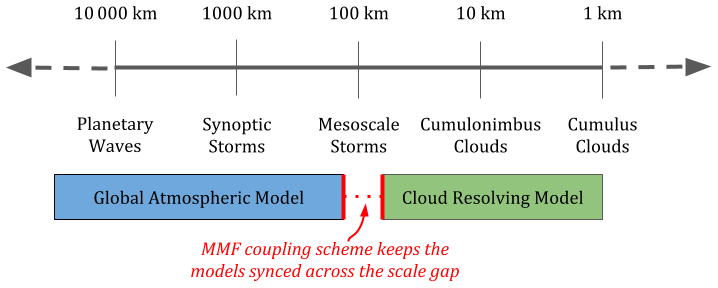
Figure 1 Schematic illustration of the scale gap created by the MMF paradigm, in which two models are coupled across a range of scales that neither can represent.

A notable trade-off of the MMF method is that there is a “scale gap” between the resolved scales of the GCM and CRM where neither model represents the relevant processes (see Fig. 1). The MMF method couples the two models through forcing and feedback tendencies formulated such that the domain mean thermodynamic state of the CRM and its parent GCM columns cannot drift apart. A related consequence of the scale gap is that the internal spatial variability of the CRM cannot be advected by the GCM flow and remain “trapped” in the CRM. Thus, the propagation of signals organized within the CRM can only happen indirectly through the coupling of the CRM domain mean (Pritchard et al., 2011).

Most MMF results in the literature use a global host model with a finite-volume grid that produces a smooth solution (Khairoutdinov et al., 2005; Benedict and Randall, 2009). However, results from the MMF configuration of the DOE Energy Exascale Earth System Model (E3SM-MMF) revealed a strong grid-imprinting signal related to the use of the spectral element grid (Hannah et al., 2020). This problem is hypothesized to be related to “cusps” in the solution that can form due to discontinuous derivatives at the shared spectral element edges. These occasional cusps lead to noise in the vertical velocity field (Herrington et al., 2019b), which the embedded CRMs in E3SM-MMF are notably more sensitive to compared to traditional convective parameterizations. The analysis of Hannah et al. (2020) did not relate the grid-imprinting signal to the trapping of CRM fluctuations, but a connection could not be ruled out.

The grid-imprinting issue in E3SM-MMFv1 is associated with the heterogeneous nature of the spectral element grid, in which element edge nodes exhibit slightly different behavior compared to interior nodes. The effects of this heterogeneity can be alleviated by putting the physics calculations on a quasi-regular finite-volume grid and mapping tendencies back to the dynamics grid similar to Herrington et al. (2019a), colloquially known as “physgrid”. The physgrid method can also make the model more efficient by using a physics grid that is coarser than the underlying dynamics grid (i.e., a 2×2 finite-volume mesh in each element), which does not qualitatively alter the model solution. A version of the physgrid that allows for regional mesh refinement was recently implemented in E3SM as described by Hannah et al. (2021), although their analysis does not include results from E3SM-MMF.

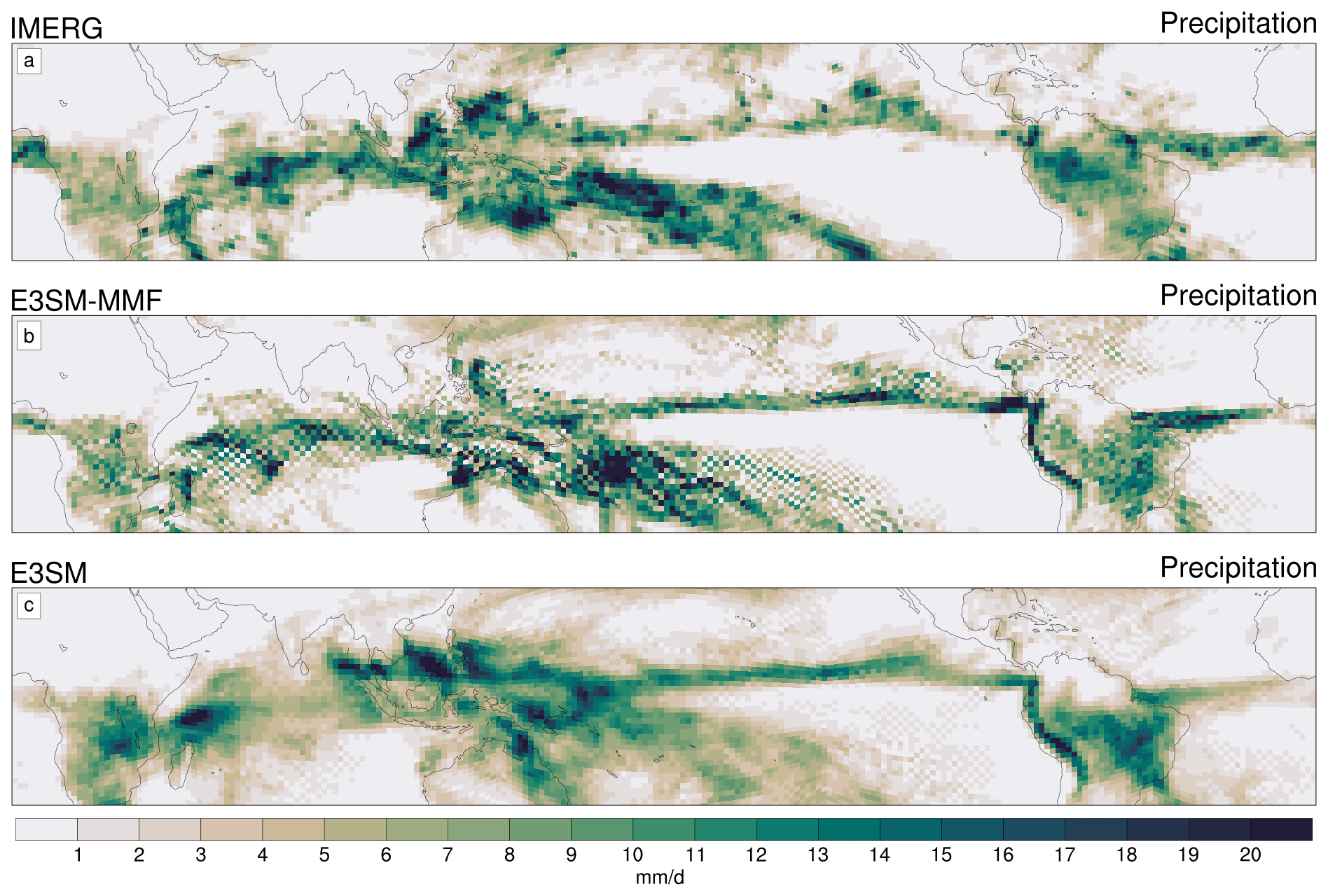
Figure 2 Single-month mean maps for an arbitrarily chosen January of precipitation data from IMERG, E3SM-MMF, and E3SMv2. Data are plotted on the native ne30pg2 physics grid using shaded polygons in order to see signals at the grid scale.

Despite the fact that E3SM-MMF running with the physgrid produces a smoother solution when compared to the previous physics grid configuration, further analysis revealed a new type of noise pattern emerges on the physics grid. This pattern resembles a “checkerboard” with alternating positive and negative differences relative to a localized area mean in fields related to convection on the physics grid. The checkerboard pattern in E3SM-MMF precipitation can be seen alongside satellite data in the 1-month mean maps from an arbitrarily chosen January in Fig. 2a, b. Visual inspection of many fields and averaging windows reveals that the pattern is most apparent in subtropical regions and is detectable on many timescales, including, alarmingly, averages of 5–10 years. The checkerboard signal also depends on the vertical level, with the strongest signals occurring at the levels where shallow clouds are present. Note that the checkerboard pattern is often obscured in data that have been regridded to a traditional equiangular grid for analysis, and thus it is important to consider data on the native cube sphere grid.

The robustness of the checkerboard in E3SM-MMF suggests that it is not related to a realistic physical process. The MMF is unlike a typical convective parameterization, in that the CRM exhibits stochastic behavior since it does not rely on an equilibrium assumption (Jones et al., 2019). Therefore, it may not come as a surprise if the MMF solution is noisier than a traditionally parameterized model, but it is unclear how long it might take to average out a noisier solution from this type of model. The MMF scale gap described above may also be playing a role in effectively trapping CRM fluctuations and causing the checkerboard since these fluctuations cannot be advected on the global grid. However, this explanation must account for how the global model dynamics drive the processes required to sustain the pattern.

Numerous sensitivity tests have been conducted to rule out early hypotheses such as erroneous code in the physgrid mapping and unstable parameter values for hyperviscosity in the spectral element dynamical core. The results of these tests are difficult to explore thoroughly because they all yield a null result in which the checkerboard signal does not appear to diminish significantly. Therefore, in order to probe the nature of this issue more deeply we will focus here on developing a method to objectively quantify various aspects of the checkerboard pattern rather than relying on visual inspection to detect and compare the prevalence of the checkerboard between different model configurations.

Interestingly, the recently released version 2 of E3SM (E3SMv2) has also been found to produce a similar checkerboard pattern as E3SM-MMF, albeit one that is much less severe (see Fig. 2c). The previous version of E3SM does not exhibit any noticeable systematic unphysical patterns in long-term means. Sensitivity experiments revealed that the E3SMv2 checkerboard is a direct consequence of a new convective trigger that relies on CAPE generated by the large-scale dynamics (Xie et al., 2019), known as the “DCAPE trigger”, and thus we will include additional analysis of E3SMv2 with this option disabled to quantify its impact.

The goal of this paper is to quantitatively document the nature of the checkerboard pattern in E3SM-MMF and E3SMv2. To do this we devise a method to objectively detect and catalog patterns of adjacent neighbors on a grid and compare the occurrence of these patterns to satellite observations. The pattern detection method and model data are detailed in Sect. 2, followed by the results of the detection analysis in Sect. 3. Conclusions are presented in Sect. 4.

2 Methods

An especially difficult aspect of examining the checkerboard problem is that the signal is generally weak compared to realistic weather variations. This makes it impossible to cleanly separate the checkerboard signal from synoptic-scale features, which are often superimposed. So rather than trying to isolate the occurrence of a clear checkerboard pattern, we choose to take a broader approach and catalog all possible patterns of relative values in a local neighborhood of adjacent points for every point on the model grid. This allows us to objectively determine if any number of patterns are occurring more frequently than what we find for observed data remapped to the same grid.

2.1 Adjacent neighbor identification

The first step to cataloguing patterns in the data is to identify the adjacent neighbors of each cell to define each local “neighborhood”. This is done on the quadrilateral cells of the finite-volume physics grid using connection information to identify cells that share a cell edge or corner. Initially, a distance-based nearest-neighbor method was employed, but this was problematic in regions where the cube–sphere grid is distorted by the projection onto the sphere. The cell connection information can be generated through a brute force comparison of cell corner locations to identify cells that share a corner. A shared edge can then be easily defined when two cells share two corners.

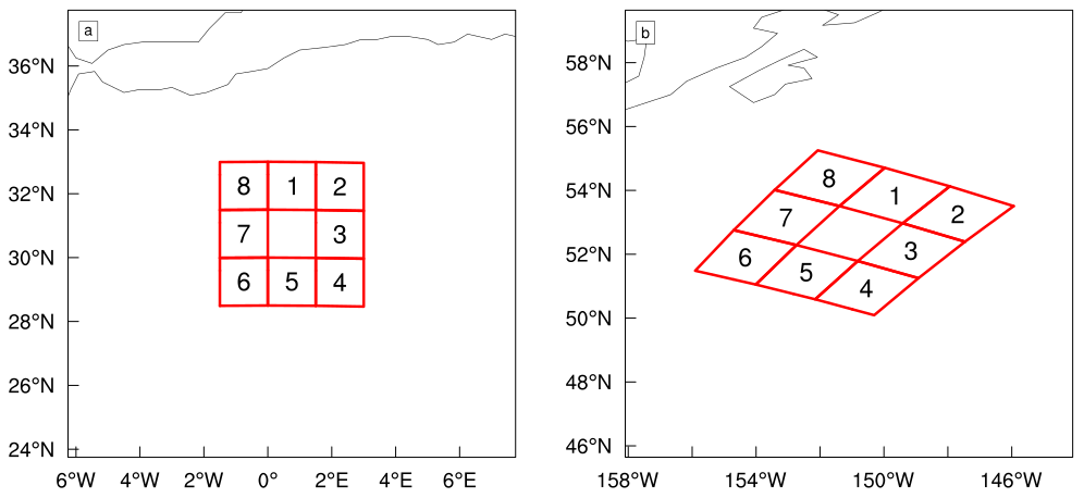
Figure 3 Examples of the nearest-neighbor detection algorithm (see text). Numbers indicate the ordering of adjacent neighbors such that the northernmost edge neighbor is first in the sequence with a clockwise order.

After identifying the adjacent neighbors to a given cell, the neighbors are sorted by the great circle bearing between the central point and each neighbor, putting the northernmost edge point first (see Fig. 3a). This ordering ensures consistency when comparing local neighborhoods across different areas of the global grid that experience different amounts of distortion from the spherical projection (Fig. 3b). Ordering the neighbors by bearing in this manner is also useful for defining the neighbor states as a sequence (see Sect. 2.2). The same method works trivially for equiangular grids. Note that for cubed sphere data we ignore points located to the cube corners because these only have seven adjacent neighbors and cannot be directly compared to the rest of the grid using the methods described below.

2.2 Pattern detection

Once we have identified the local adjacent neighborhood of a given center point, we need a way to catalog the various neighborhood state patterns. In order to make the pattern detection tractable we simplify the neighborhood state by calculating differences from the center cell and then encode the adjacent neighbor differences as binary values, with 0 for values less than or equal to the center value and 1 otherwise. Note that the center point is excluded from the binary sequence for convenience, which would otherwise complicate the pattern interpretation and partial checkerboard identification (see below). Our experience suggests that these methodology choices are arbitrary and do not affect our conclusions.

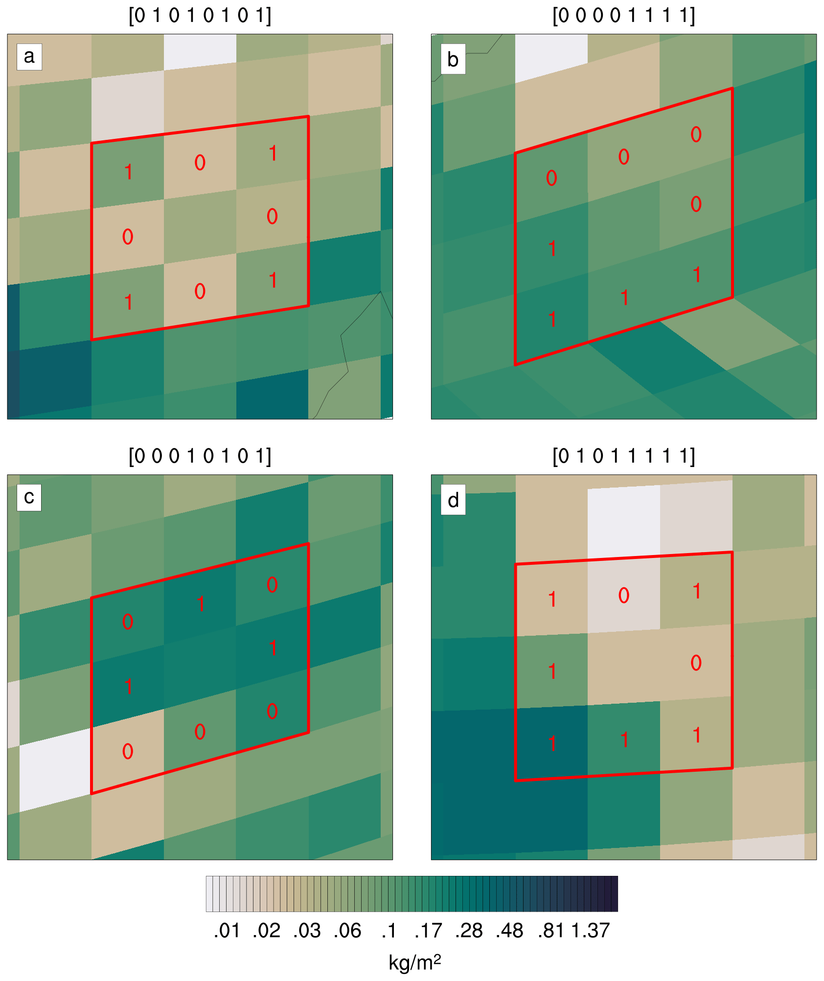
Figure 4 Examples of the patterns identified in daily snapshots of liquid water path from E3SM-MMF corresponding to the pattern examples in Table 1. Cells are labeled with a “0” for values less than or equal to the center value and “1” otherwise. Note that a logarithmic spacing is used for the color levels.

For a given neighborhood state we are left with a sequence of eight binary values corresponding to the adjacent neighbors ordered in a clockwise fashion. A pure checkerboard pattern can now be easily identified as an alternating binary sequence. The smoothness of a pattern can also be inferred from the variations of this sequence. Examples of different neighborhood patterns are shown in Table 1 with corresponding examples shown in Fig. 4 using daily mean snapshots of liquid water path from the E3SM-MMF simulation described below.

Table 1 Examples of binary sequences that describe the relative states of the eight adjacent neighbors relative to a given center point on a rectilinear grid (see text).

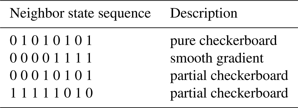
Our pattern detection method gives us a simple way to catalog patterns in a local neighborhood, including a pure checkerboard. However, there are several sets of unique patterns that are functionally equivalent. For example, the sequences [00001111] and [00011110] both describe a smooth gradient across the neighborhood, but in most cases we do not need to distinguish these as distinct patterns because they are equivalent if we allow the pattern to be rotated. If we do not account for rotational symmetry then there are 256 possible patterns of neighbor states, whereas accounting for rotational symmetry reduces the number of possible patterns to 36.

One case where we want to ignore rotational symmetry is when exploring the pure checkerboard pattern. The patterns [01010101] and [10101010] represent different “phases” of the pure checkerboard pattern, which should occur with roughly the same frequency at all points if the model solution is translationally invariant. Compositing all points with either phase may also be useful for exploring the mechanisms that drive the signal (not shown).

As we will see later in Fig. 7, despite the seemingly widespread checkerboard in long-term means, the occurrence of a pure checkerboard pattern is surprisingly infrequent in daily mean data when compared to other possible neighborhood patterns. This makes sense given that the checkerboard pattern will often coexist with synoptic weather features that mask the signal over short timescales. To overcome this complication it is insightful to focus on patterns that contain only part of the full checkerboard pattern. To do this we identify neighbor state patterns that contain an alternating binary sequence of length four or more and consider these to be “partial checkerboard” cases (see Table 1). A stricter definition of partial checkerboard that requires a longer alternating sequence does not qualitatively change our results (not shown).

The occurrence of any pattern will change depending on the timescale of the data. This may seem obvious if we were to compare monthly and daily means, but differences are also noticeable when comparing the results of sub-daily and daily data. In order to facilitate comparison with satellite observations we will only use daily data for the pattern detection.

2.3 Model description

E3SM was originally forked from the NCAR CESM (Hurrell et al., 2013), but all model components have undergone significant development since then (Golaz et al., 2019; Xie et al., 2018). The dynamical core uses a spectral element method on a cubed-sphere geometry (Ronchi et al., 1996; Taylor et al., 2007). Physics calculations, including the embedded CRMs in E3S-MMF, are performed on a finite-volume grid that is slightly coarser than the dynamics grid but more closely matches the effective resolution of the dynamics (Hannah et al., 2021).

In a similar fashion to E3SM, the MMF configuration of E3SM (E3SM-MMF) was originally adapted from the super-parameterized CAM (SP-CAM; Khairoutdinov et al., 2005). E3SM-MMF has also undergone significant development, but the model qualitatively reproduces the general results previously published studies (Hannah et al., 2020). The embedded CRM in E3SM-MMF is adapted from the System for Atmospheric Modeling (SAM) (Khairoutdinov and Randall, 2003). Microphysical processes are parameterized with a single-moment scheme, and sub-grid scale turbulent fluxes are parameterized using a diagnostic Smagorinsky-type closure. Aerosol concentrations are prescribed with present day values. The embedded CRM in E3SM-MMF uses a two-dimensional domain with 64 CRM columns in a north–south orientation and 1 km horizontal grid spacing. Note that various sensitivity tests have shown that the details of the CRM domain configuration do not qualitatively affect our results (not shown).

Aside from the difference in how convection is treated, the configurations of E3SM-MMF and E3SMv2 differ in several ways. The stability of E3SM-MMF is noticeably improved by reducing the global model physics time step from 30 to 20 min. The 72 layer vertical grid of E3SMv2 was also found to be problematic for the performance of E3SM-MMF because thin layers near the surface necessitate a 5 s CRM time step for numerical stability. Therefore, the E3SM-MMF simulation shown here uses an alternative 50-layer vertical grid that allows a longer 10 s CRM time step. A final stability concern has to do with high-frequency oscillations of various atmospheric quantities near the surface, such as wind and temperature. Both models exhibit these oscillations, but they render E3SM-MMF much more susceptible to crashing. A temporal smoothing of surface fluxes with a 2 h timescale is used to address this problem, which does not have any notable impact on the model climate. These configuration choices and others, such as the CRM grid parameters, have been explored in numerous sensitivity tests, but in all cases they were found to have a negligible impact on the checkerboard signal in E3SM-MMF (not shown).

2.4 Model simulations

All simulations are run for 5 years using 85 nodes of the NERSC Cori-KNL computer (5400 MPI ranks). While hardware threading can be utilized outside of the CRM calculations, we did not employ threading in the simulations presented here. The use of 5-year simulations is common practice in model evaluation and is a trade-off between computational cost and signal-to-noise ratio. The global cubed sphere grid was set at ne30pg2 (30×30 spectral elements per cube face and 2×2 finite-volume physics cells per element), which roughly corresponds to an effective grid spacing of 150 km. The model input data for quantities such as solar forcing, aerosol concentrations, and land surface types, are derived from a 10-year climatology over 1995–2005 to be representative of climatological conditions around 2000. Sea surface temperatures were similarly prescribed using monthly climatological values that are temporally interpolated to give a smooth evolution (Taylor et al., 2000).

2.5 Satellite data

We are interested in characterizing the checkerboard patterns in satellite data as a way to determine the degree of realism in the model data, and thus the specific time period of satellite data used for analysis is arbitrary. We choose to use daily mean data over 2005–2009. Since the checkerboard pattern is most visible in cloud liquid water path and precipitation fields, we use comparable satellite estimates of these fields to provide a baseline of the spatial distribution of these quantities.

Satellite estimates of cloud liquid water path are provided by the Multisensor Advanced Climatology of Liquid Water Path (MAC-LWP) data product (Elsaesser et al., 2017). We use a daily resolution version of the product (McCoy et al., 2020), with LWP estimates provided on a $\mathrm{1.0}\times \mathrm{1.0}{}^{\circ }$ equiangular grid that is then regridded to the ne30pg2 grid used by the model. MAC-LWP additionally provides total (cloud plus precipitating) liquid water path estimates (TLWP), and we use TLWP to create a gridded quality control mask that hashes regions for which the ratio of LWP to TLWP is less than 0.6, broadly following the recommendation in Elsaesser et al. (2017). Hashed regions envelope grid boxes for which LWP estimates exhibit substantial uncertainty (and potential systematic bias) due to errors in isolating and quantifying the cloud liquid water radiometric signature from that of the total liquid water radiometric signature in microwave retrievals.

The Global Precipitation Measurement (GPM) mission, the successor to the Tropical Rainfall Measurement Mission (TRMM), was launched in 2014 with the goal of producing accurate and reliable estimates of global precipitation with all available data TRMM and GPM eras (Hou et al., 2014). The Integrated Multi-satellite Retrievals for GPM (IMERG) combines several satellite data sets to produce an integrated rainfall data product that has proven to perform well in various regions (Anjum et al., 2018; Kim et al., 2017). Daily mean IMERG data is available on a $\mathrm{0.1}\times \mathrm{0.1}{}^{\circ }$ grid, which is much finer than the grid used for the model simulations used here. To facilitate direct comparison, we regrid the IMERG data to the ne30pg2 model grid, as well as a $\mathrm{1.0}\times \mathrm{1.0}{}^{\circ }$ equiangular grid to match the MAC-LWP data.

3 Results

In this section we will present the results of the pattern detection algorithm described in Sect. 2.2. We will focus on providing a broad comparison of how various patterns occur in each data set, as well as an assessment of persistence of partial checkerboard patterns.

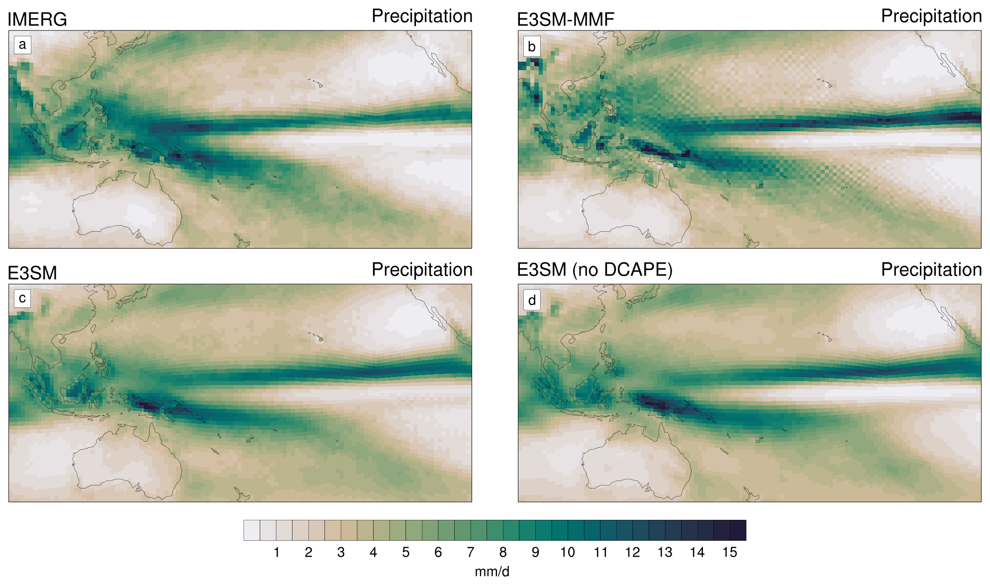
Figure 5 Maps of 5-year mean precipitation for IMERG, E3SM-MMF, E3SMv2, and E3SMv2 with the DCAPE trigger disabled.

Figure 6 Maps of 5-year mean liquid water path for MAC-LWP, E3SM-MMF, E3SMv2, and E3SMv2 with the DCAPE trigger disabled. Hashing indicates regions for which MAC cloud liquid water path is more uncertain, as described in Sect. 2.2.

3.1 Checkerboard climatology

Figures 5 and 6 show 5-year average maps of precipitation and cloud liquid water path centered over the tropical Pacific using all data sets on the ne30pg2 grid. The Pacific region was intentionally used because it is often where the most obvious checkerboard signal can be seen in E3SM-MMF. The satellite data from IMERG and MAC-LWP do not indicate any systematic noise on the ne30pg2 grid as we expect (Figs. 5–6a). Hashed regions in Fig. 6a indicate where time-averaged MAC-LWP data are more uncertain due to the prevalence of deep convection and increased precipitation water that makes it difficult to determine accurate estimates of cloud-only liquid water paths. The checkerboard pattern is immediately evident in E3SM-MMF data, along with all the standard climatological features we expect, such as the tropical convergence zones (Figs. 5–6b).

It is not immediately obvious that either E3SMv2 case exhibits any checkerboard signal in the long-term means, but there are slight indications that the case with the DCAPE trigger disabled produces a smoother climatology (Figs. 5–6d). Part of what hides the checkerboard signal in Figs. 5–6c is the choice of color bar, along with the fact that the checkerboard signal in E3SMv2 is weak compared to E3SM-MMF. The checkerboard in E3SMv2 can be made more visually apparent in both of these fields when using a color bar with a logarithmic scale (not shown).

The results of the pattern detection algorithm contain a wealth of information that is challenging to condense. Visualizing the fractional occurrence of each separate pattern is very difficult to parse and understand, even after accounting for rotational symmetry. Alternatively, we can combine patterns based on the number of local extrema in the binary neighborhood pattern sequence. This approach simply counts the number of ones surrounded by zeros and vice versa. A pure checkerboard pattern has eight local extrema, and a lower number of extrema indicates a less noisy state in the local neighborhood. Note that local extrema counts of six and seven are not possible in a binary sequence of length eight.

Figure 7 (a, c) Fractional occurrence of neighborhood patterns combined according on the number of local extrema (see text) over the region 0–30^∘ N, 140–220^∘ E (see inset map) for 5 years of satellite and model data. Results for IMERG precipitation and MAC liquid water path are shown on a 1×1^∘ grid and the ne30pg2 grid used by the model for direct comparison. (b, d) Difference in fractional occurrence relative to satellite data on the ne30pg2 grid.

Figure 7a, c shows the result of combining patterns by the number of local extrema using liquid water path and precipitation data from the northwest tropical and subtropical Pacific. For each satellite data set, we have included results from both ne30pg2 and $\mathrm{0.1}\times \mathrm{0.1}{}^{\circ }$ grids to reveal any influence of the remapping. The difference in each fractional occurrence value relative to the satellite data on the ne30pg2 grid is shown in Fig. 7b, d.

Figure 7 makes it clear that the occurrence of the pure checkerboard (eight local extrema) is quite rare relative to the other patterns, and E3SM-MMF produces the most frequent occurrence of this pattern. However, E3SM-MMF has an even larger prevalence of patterns with three, four, and five local extrema relative to all other data sets. Inversely, smooth patterns with no local extrema are produced much less often in E3SM-MMF than any other data set. This indicates that E3SM-MMF has a less smooth solution in general, and also illustrates the importance of considering partial checkerboard patterns rather than only looking for a pure checkerboard.

Figure 7 shows an interesting distinction between our two E3SMv2 simulations. The E3SMv2 case with the DCAPE trigger shows a higher occurrence of noisier patterns with more local extrema and a lower occurrence of pattern with no local extrema. Thus, the results are similar to E3SM-MMF but with smaller differences relative to the satellite data. Conversely, E3SMv2 has a much smoother solution without the DCAPE trigger, as it has a relatively low occurrence of noisier patterns and a relatively high occurrence of the smoother patterns compared to satellite data.

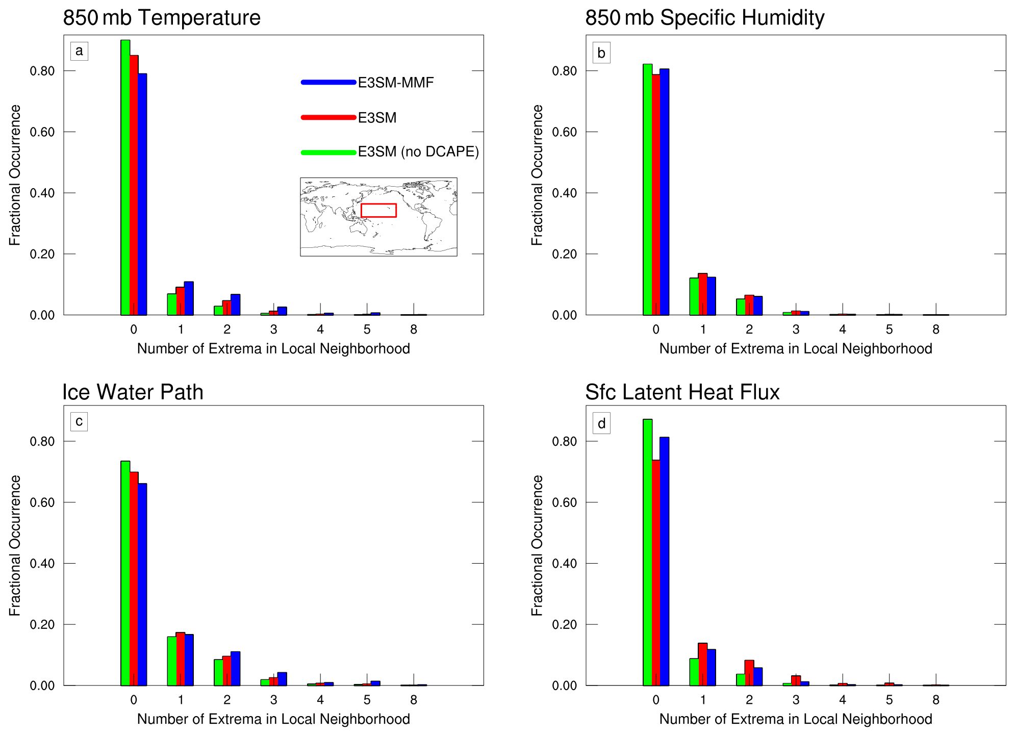
Figure 8 Similar to Fig. 7, showing fractional occurrence of neighborhood patterns over the region 0–30^∘ N, 140–220^∘ E for various model variables that do not exhibit a checkerboard pattern, specifically 850 mb temperature (a), 850 mb zonal wind (b), ice water path (c), and surface latent heat flux (d).

Figure 8 shows a similar analysis to Fig. 7 using model data for various other quantities. These variables were chosen because they do not appear to exhibit any checkerboard signal from visual inspection of map plots of various averaging timescales (not shown), and Fig. 8 shows that the pattern detection algorithm can quantitatively confirm this observation. Ice water path is a slight exception because E3SM-MMF does exhibit a weak amount of checkerboard signal in this field. However, the occurrence of the noisier patterns is much smaller than that in Fig. 7. Despite this analysis not being able to tell us anything about the checkerboard pattern, it is interesting to note that it supports our previous observation that both E3SMv2 and E3SM-MMF are noisier than E3SMv2 without the DCAPE trigger, although we cannot say which result is more realistic.

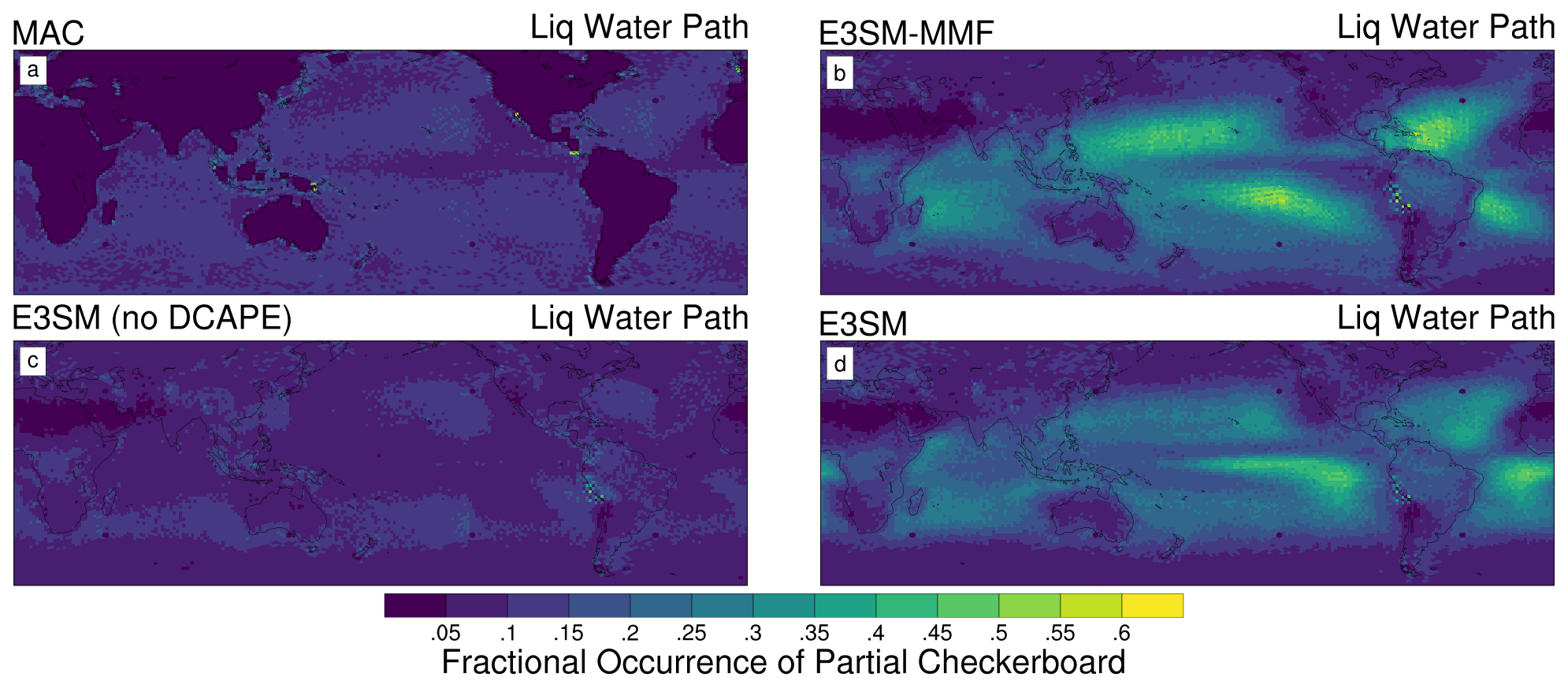
Figure 9 Maps of fractional occurrence of partial checkerboard patterns (see text) for MAC-LWP (a), E3SMv2 without DCAPE (b), standard E3SMv2 with DCAPE (c), and E3SM-MMF (d). All data are on the ne30pg2 grid.

Figure 9 shows maps of fractional occurrence for partial checkerboard patterns in liquid water path data. The more prevalent occurrence of partial checkerboard is seen in the subtropical regions from E3SMv2 and E3SM-MMF. The regions that stand out are in line with what we expect from how the checkerboard pattern is revealed in long-term averages, such as Fig. 6. Interestingly, the E3SMv2 case without DCAPE also shows that the subtropics are very slightly noisier than other regions, but the significance of these regional differences is difficult to assess since the occurrence of partial checkerboard patterns is so low.

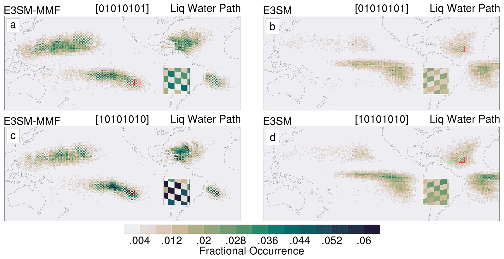
Figure 10 Maps of each unique phase of the pure checkerboard pattern in E3SM-MMF (a, c) and E3SMv2 (b, d). The map inset shows an arbitrarily chosen small region to highlight the “out of phase” nature of the phases, indicating a lack of translational invariance.

3.2 Translational invariance of the pure checkerboard

A curious property of the checkerboard pattern in E3SM-MMF is that it seems to be spatially “locked”, allowing it to be clearly seen in multi-year averages. This suggests that the localized statistics of the model state are not translationally invariant, such that certain columns exhibit fundamentally different behavior from their immediate neighbors. Such a discontinuity in statistics should be especially alarming in regions with roughly homogeneous large-scale dynamics and surface boundary conditions, such as the subtropical regions of the central Pacific. To illustrate this more clearly, Fig. 10 shows the fractional occurrence of each unique phase of the pure checkerboard pattern for E3SM-MMF and E3SMv2. A similar plot that combines both checkerboard phases (not shown) reveals subtropical regions of elevated occurrence with a smooth spatial texture. However, when the phases are plotted separately for E3SM-MMF, we see that the pattern of occurrence itself reveals a checkerboard pattern (Fig. 10a, c). Furthermore, comparing the inset maps of Fig. 10 reveals that the checkerboard patterns of the pure checkerboard phase occurrence are out of phase with each other. This shows that the model solution is indeed not translationally invariant in the regions where checkerboard is detected.

Figure 10b, d illustrates how the checkerboard signal is less persistent in E3SMv2 and exhibits less of a departure from a translationally invariant solution. The checkerboard phase occurrence still exhibits a degree of checkerboard pattern itself, but this signal is less robust than E3SM-MMF. This suggests that the processes associated with the DCAPE trigger that conspire to produce the checkerboard pattern are less prone to becoming spatially locked.

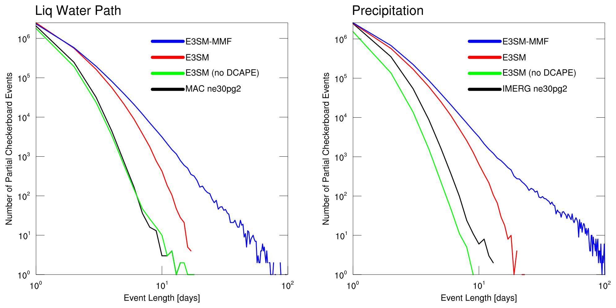
Figure 11 Histogram of the event length, with events defined as continuous periods with partial checkerboard neighborhood state. Data were restricted to oceanic points equatorward of 60^∘ latitude in both hemispheres for all 5 years that were available.

3.3 Checkerboard pattern persistence

The mere existence of a partial checkerboard pattern does not necessarily mean that the signal is unphysical, but an unnaturally persistent pattern should not be considered realistic for a moist, convecting atmosphere. To investigate how persistent the partial checkerboard patterns are we consider all valid oceanic data points (points with oceanic neighbors) between 60^∘ S and 60^∘ N and identify periods where a local neighborhood stays in a state of partial checkerboard. Figure 11 shows a histogram of the length of all these events for liquid water path and precipitation. In both variables we see that E3SM-MMF and E3SMv2 show a larger number of events of any length when compared to satellite data and E3SMv2 without the DCAPE trigger. E3SM-MMF exhibits events that last nearly 100 d, which is not seen in any other data set. E3SMv2 without DCAPE behaves similar to satellite observations in this respect, further supporting the conclusion that the DCAPE trigger is the sole cause of the checkerboard signal in E3SMv2. The tendency to produce relatively long-lived partial checkerboard events in E3SMv2 and E3SM-MMF illustrates how the checkerboard becomes imprinted onto the climatology through persistent checkerboard signals superimposed on the typical fluctuations from weather.

3.4 Variance trapping in E3SM-MMF

The analysis thus far is sufficient to confirm that the checkerboard pattern in E3SMv2 is a direct result of the DCAPE trigger. We believe this is due to a feedback mechanism in which convectively active cells of the checkerboard pattern experience resolved upward motion and further CAPE generation from dynamics, and the adjacent neighbors experience a stabilizing effect from the subsiding portion of the local circulation that causes the DCAPE trigger to suppress convection. Without the DCAPE trigger the deep convection scheme is notorious for launching convection too often, which prevents this feedback from becoming established. This hypothesis is loosely supported by experiments with alternate calculations of CAPE generation for the trigger condition, such as including radiation (not shown).

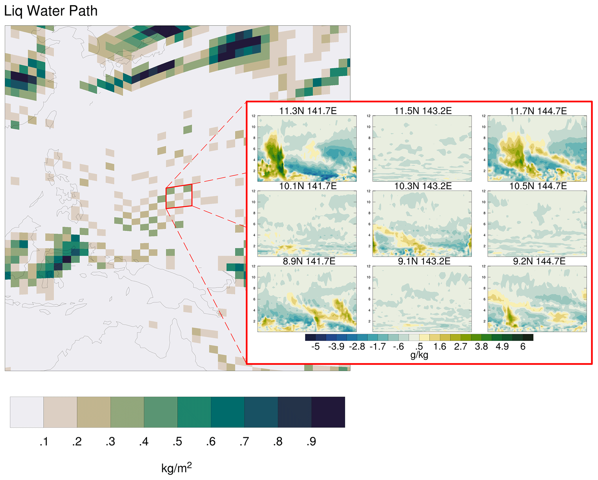
Figure 12 Instantaneous snapshot of tropical western Pacific liquid water path and CRM water vapor field for a select region exhibiting a checkerboard pattern for an arbitrarily selected day in boreal summer.

Finding an explanation for the checkerboard signal in E3SM-MMF is less straightforward. Figure 12 shows a representative snapshot of liquid water path on the global grid and a localized group of CRM water vapor fields arbitrarily selected from a region exhibiting a checkerboard pattern shown as anomalies from the horizontal mean at each level of the CRM domain. There is a clear correspondence between the liquid water path on the global grid and amplitude of the CRM-scale fluctuations. The relatively dry cells of the checkerboard pattern exhibit very little variation in the water vapor field and similarly exhibit very little variation in CRM wind anomalies. This contrast of CRM fluctuations between adjacent neighbors is evident across checkerboard regions even when a synoptic weather system is moving through.

The persistence of fluctuations in one CRM and suppression of fluctuations in a neighboring CRM suggest that these fluctuations have become “trapped” in such a way that they are not easily dissipated. It is reasonable to speculate that these trapped fluctuations can have a perpetual influence on neighboring cells. In general, moist convection often produces heating and drying to balance cooling and moistening tendencies produced by other processes, such as large-scale dynamics, radiation, and surface fluxes. Thus, a relatively “active” CRM might produce a sufficiently dry, stable state that could suppress convective activity in a neighboring CRM when advected by the dynamics. Similarly, a relatively “inactive” CRM might allow convective instability to increase through cooling and moistening by other processes as this air mass was being advected.

4 Conclusions

In this study we have presented a novel pattern detection method to investigate a checkerboard pattern in cloud-related variables over subtropical ocean regions in E3SM-MMF and E3SMv2. Using satellite data of liquid water path and precipitation as a baseline, our analysis shows that certain patterns associated with a noisier state occur too often in localized regions and are too persistent. These results support the conclusion that the checkerboard is clearly unphysical. The signal in E3SMv2 is caused by the recently added convective trigger based on dynamically generated CAPE (DCAPE), whereas the source of the checkerboard in E3SM-MMF is seemingly related to “trapping” of cloud-scale fluctuations within the embedded cloud resolving model (CRM).

We have stopped short of providing a detailed analysis of the feedback mechanisms that perpetuate the pattern for several reasons. An examination of the vertically resolved moisture budget would likely help us to understand why the checkerboard persists, but this is quite difficult to do on the native grid, especially given the fact that dynamics calculations are done on a different grid (i.e., the np4 spectral element grid). A simple composite of CRM forcing and feedback terms in E3SM-MMF also seems like it would be illuminating, but given the contamination of weather variations it is very difficult to isolate the moment that the checkerboard comes into existence. Thus, a composite of synoptic-scale processes for checkerboard regions can only show the balance of processes between relatively cloudy and non-cloudy cells that make up the checkerboard, without being able to clearly isolate how one cell influences its adjacent neighbors.

Despite not being able to fully understand the fundamental mechanism behind the checkerboard signal, there are several outstanding questions to which we can provide a speculative answer. The CRM instances of E3SM-MMF are completely independent, and thus the dynamics of the global model are clearly important for setting up the pattern via advection, and the physics calculations must be responsible for making it persist locally. The prevalence of checkerboard signals in subtropical regions suggests that unrelenting intensity of the trade winds might be providing the ideal environment for these feedbacks to persist. The subtropical regions might also be ideal because there is less influence from synoptic systems relative to other weather regimes.

Interestingly, the checkerboard signal is not detected over land regions, and the reason for this is unclear. The use of prescribed sea surface temperature might seem like a potential complication because the surface temperature cannot respond to the local convection like it does over land, but tests with a fully coupled ocean still exhibit checkerboard patterns (not shown). Presumably, the land vs. ocean contrast has something to do with smaller heat capacity of the land surface and stronger diurnal cycle of surface fluxes, but more work is needed to clarify this hypothesis.

An obvious question to ask is whether the checkerboard problem is isolated to E3SM-MMF or if all MMF models exhibit a version of the same problem. Additional experiments were done with the NCAR super-parameterized CAM (SP-CAM) to investigate this question (not shown). While SP-CAM and E3SM-MMF share a lot of features, the dynamical cores have diverged significantly over recent years, including the one used for the spectral element grid. Experiments with SP-CAM used both the finite-volume and spectral element dynamical core options and the checkerboard pattern was detected, but with a much lower frequency of occurrence. This result is very puzzling, but we suspect it has something to do with the difference in the dynamical cores, perhaps related to the choice of whether to use “dry” or “full” pressure.

The final outstanding question to pose is how this problem should be addressed. For E3SMv2, the DCAPE trigger needs to be revisited, and a simple solution of adjusting the trigger threshold might provide a way to address the issue, but additional sensitivity experiments are needed. Preliminary experiments that modify the DCAPE trigger to include CAPE generation by radiation show a notable reduction in the checkerboard signal (not shown). Presumably, this is due to radiative cooling being able to more efficiently generate CAPE in the less cloudy cells of the checkerboard.

Our current hypothesis is that the checkerboard pattern in E3SM-MMF is due to the “trapping” of CRM fluctuations, which is essentially a “design flaw” of the MMF concept associated with the scale gap illustrated in Fig. 1. In the real atmosphere, these relatively small-scale fluctuations on the scale of individual clouds would be advected by the larger-scale flow in which they are embedded, but this process is missing from the MMF. We cannot fully include this process without discarding the scale gap and producing a global CRM, which would eliminate the computational advantages of the MMF. Alternatively, we can transport CRM fluctuations by encoding this information into a bulk variance tracer that can be advected on the global grid. A method for this “CRM variance transport” is presented in another publication (Hannah and Pressel, 2022), which demonstrates that it is effective at eliminating the checkerboard patterns in the E3SM-MMF climatology.