the Creative Commons Attribution 4.0 License.
the Creative Commons Attribution 4.0 License.
 | 21 Jul 2022
SurEau-Ecos v2.0: a trait-based plant hydraulics model for simulations of plant water status and drought-induced mortality at the ecosystem level
Julien Ruffault
François Pimont
Hervé Cochard
Jean-Luc Dupuy
Nicolas Martin-StPaul
A widespread increase in tree mortality has been observed around the globe, and this trend is likely to continue because of ongoing climate-induced increases in drought frequency and intensity. This raises the need to identify regions and ecosystems that are likely to experience the most frequent and significant damage. We present SurEau-Ecos, a trait-based, plant hydraulic model designed to predict tree desiccation and mortality at scales from stand to region. SurEau-Ecos draws on the general principles of the SurEau model but introduces a simplified representation of plant architecture and alternative numerical schemes. Both additions were made to facilitate model parameterization and large-scale applications. In SurEau-Ecos, the water fluxes from the soil to the atmosphere are represented through two plant organs (a leaf and a stem, which includes the volume of the trunk, roots and branches) as the product of an interface conductance and the difference between water potentials. Each organ is described by its symplasmic and apoplasmic compartments. The dynamics of a plant's water status beyond the point of stomatal closure are explicitly represented via residual transpiration flow, plant cavitation and solicitation of plants' water reservoirs. In addition to the “explicit” numerical scheme of SurEau, we implemented a “semi-implicit” and “implicit” scheme. Both schemes led to a substantial gain in computing time compared to the explicit scheme (>10 000 times), and the implicit scheme was the most accurate. We also observed similar plant water dynamics between SurEau-Ecos and SurEau but slight disparities in infra-daily variations of plant water potentials, which we attributed to the differences in the representation of plant architecture between models. A global model's sensitivity analysis revealed that factors controlling plant desiccation rates differ depending on whether leaf water potential is below or above the point of stomatal closure. Total available water for the plant, leaf area index and the leaf water potential at 50 % stomatal closure mostly drove the time needed to reach stomatal closure. Once stomata are closed, resistance to cavitation, residual cuticular transpiration and plant water stocks mostly determined the time to hydraulic failure. Finally, we illustrated the potential of SurEau-Ecos to simulate regional drought-induced mortality over France. SurEau-Ecos is a promising tool to perform regional-scale predictions of drought-induced hydraulic failure, determine the most vulnerable areas and ecosystems to drying conditions, and assess the dynamics of forest flammability.
- Article
(3569 KB) - Full-text XML
- BibTeX
- EndNote


Forests across many regions worldwide are experiencing record-breaking droughts followed by widespread increase in climate-driven disturbance events, including tree mortality (Allen et al., 2015; Fettig et al., 2019; Schuldt et al., 2020), wildfires (Ruffault et al., 2020; Abram et al., 2021) and insect outbreaks (Jactel et al., 2012). Droughts are likely to become more frequent and more intense over the next decades because of the global increase in temperatures and heat waves, which are coupled in some regions to changes in the hydrological cycle (Trenberth et al., 2014). Given the importance of forests for biochemical cycles and ecosystem services (Seidl et al., 2014), there is a growing need for the development of models that can simulate the response of forests to extreme drought. Process-based vegetation models can help to address these issues because they represent the mechanisms governing plant physiological responses to drought and account for the interspecific and intraspecific variations of tree traits and their acclimation to a rapidly changing climate.
The science of plant hydraulics seeks to understand the physical and physiological mechanisms driving water transport in plants. This research field has proven to be a relevant theoretical framework to study the effect of global changes on plant and the terrestrial water cycle (Choat et al., 2018; Brodribb et al., 2020). Advances in plant hydraulic modeling have accelerated over the last 2 decades (Mencuccini et al., 2019; Fatichi et al., 2016) and are used as mean to tackle diverse prediction challenges, such as tree mortality (Venturas et al., 2020; De Kauwe et al., 2020), water use efficiency (Domec et al., 2017; De Cáceres et al., 2021) or species distribution (Sterck et al., 2011). Many of these models were also designed (or reformatted) to be integrated into land surface models and improve the representation of the feedbacks between land and climate systems (Xu et al., 2016; Li et al., 2021; Kennedy et al., 2019; Christoffersen et al., 2016). Recently, modeling water transport in plants also proved to be a promising way to assess the seasonal dynamics of live fuel moisture (foliage and twigs water content, dead to live fuel ratio), a key variable for fire behavior that could play a major role in raising forests' flammability under climate warming (Ruffault et al., 2018a; Nolan et al., 2020).
Most plant hydraulic models represent water fluxes in plants through the mathematical approach of the soil–plant–atmosphere (SPA) continuum, wherein diffusion laws control the water flow through the soil, roots and leaves (Mencuccini et al., 2019). Water flow through plants is considered to be analogous to the electrical current through a circuit with a series of resistance and/or capacitance factors (Sperry et al., 1998). SPA models, however, vary widely in their complexity, some of them representing trees as a single resistance (Mackay et al., 2003; Williams et al., 1996), while others include multiple resistances and capacitances (Sperry et al., 1998; Tuzet et al., 2017; Couvreur et al., 2018). How physiological processes regulate plant transpiration also differs between SPA models (Mencuccini et al., 2019). Some models describe stomatal conductance through semi-empirical models (Christoffersen et al., 2016; Williams et al., 1996; Li et al., 2021; Feng et al., 2018), while others are based on optimality approaches (Wang et al., 2020; Sperry et al., 2017).
The SurEau SPA model was developed specifically to simulate plant desiccation under extreme drought and heat waves (Martin-StPaul et al., 2017; Cochard et al., 2021). As in other SPA models, SurEau describes the soil–plant–atmosphere system as a network of resistances and capacitances and computes water exchanges until stomatal closure. Additionally, SurEau simulates plant tissue desiccation beyond the point of stomatal closure by accounting for residual plant transpiration and the discharge of internal plant water stores (Fig. 1a). Unlike most current approaches (Xu et al., 2016; Tuzet et al., 2017), SurEau explicitly accounts for the differences in capacitance of the symplasmic and apoplasmic compartments, which can be calibrated from pressure–volume curves for the symplasm and vulnerability curves for the apoplasm. Symplasmic capacitances mostly buffer water fluxes during well-watered conditions, whereas apoplasm capacitances come into play when cavitation occurs (Fig. 1a). Thus, SurEau accounts for the leading role of cavitation in the dynamics of plant desiccation (Mantova et al., 2021) and the probability of plant mortality (Adams et al., 2017). SurEau has been successfully evaluated against field cavitation observations (Cochard et al., 2021; hereafter CPRM21), has been applied in different contexts (Lemaire et al., 2021; López et al., 2021) and has performed well in predicting plant water fluxes when compared to other plant hydraulic models (McDowell et al., 2022).
As noted in CPRM21, two characteristics of SurEau impede its use for large-scale ecological applications or its integration into terrestrial biosphere models. First, SurEau requires a high number of parameters because of its detailed representation of plant architecture and the mechanisms involved in plant water exchanges. The second limitation of SurEau is its high computation time, which is partly due to the use of a first-order “explicit” numerical scheme to compute water flows. This scheme requires that variations in water quantities be computed at very small time steps to avoid numerical instabilities due to the Courant–Friedrichs–Lewy condition (CFL; Dutykh, 2016). A numerical method has been proposed to overcome these instabilities and increases the time step (Xu et al., 2016; Tuzet et al., 2017), but this is not directly compatible with SurEau's specificities regarding capacitances and cavitation. Moreover, knowledge regarding numerical physics and methods for simulation have seldom been applied to plant hydraulics.
We present SurEau-Ecos, a new SPA model meant to improve the predictions of ecosystems' transpiration, desiccation and drought-induced mortality at scales from stand to region. SurEau-Ecos draws on the physiological and physical framework of SurEau while limiting the number of parameters and reducing computational cost. In the following sections, we first describe the principles, functioning, main equations and numerical schemes of SurEau-Ecos. Second, we compare simulations produced with three numerical schemes (explicit, semi-implicit and implicit) in terms of prediction stability and computing time. Third, we further describe the differences in plant hydraulic architecture between SurEau-Ecos and SurEau (CPRM21) and their impacts on simulation results. Fourth, we perform a global sensitivity analysis of tree desiccation dynamics to the main SurEau-Ecos input, i.e., plant hydraulic traits and stand and soil parameters. Fifth, we illustrate the potentialities which SurEau-Ecos will provide by running prospective simulations of hydraulic failure probability at the regional scale under changing climate.
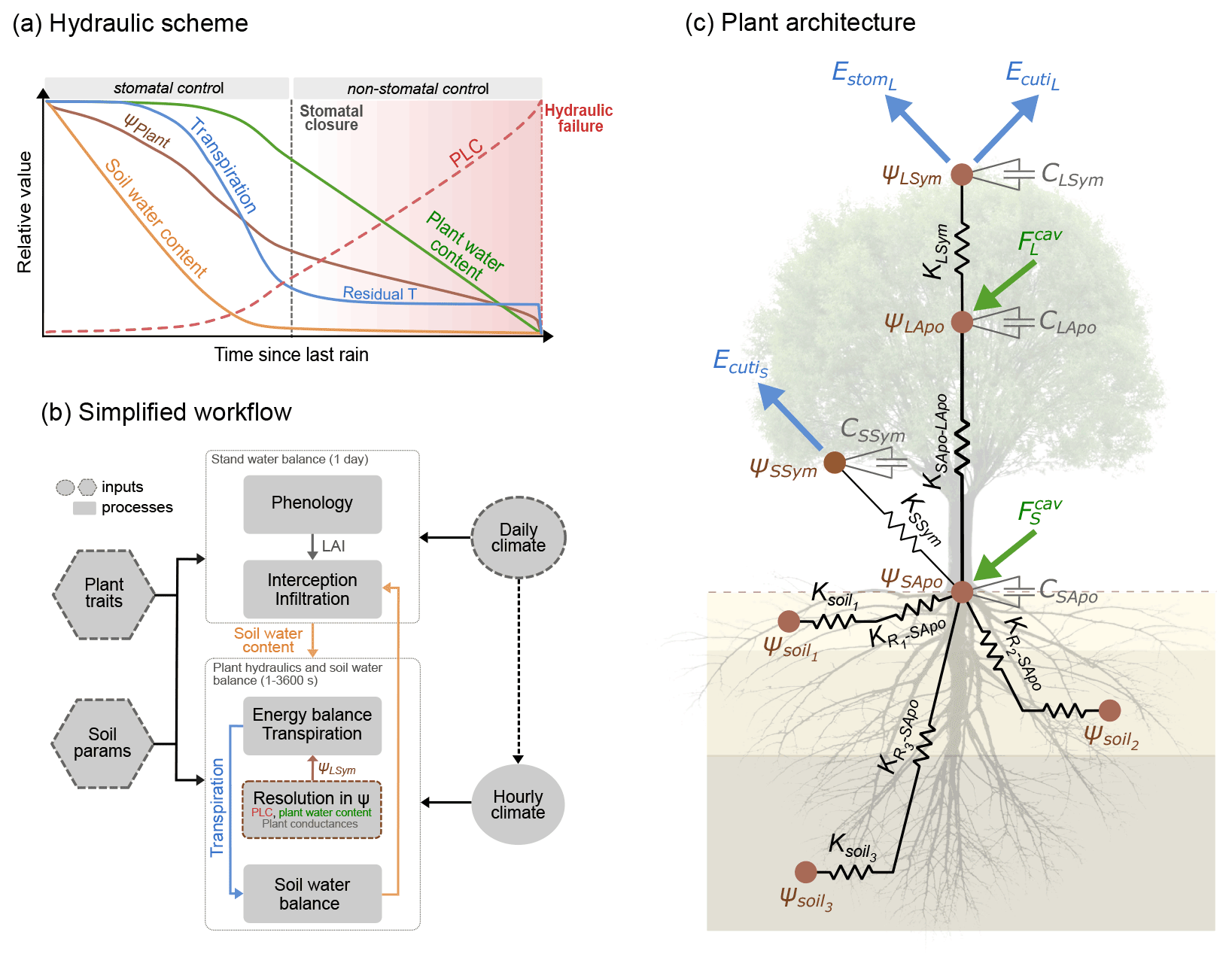
Figure 1Overview of the SurEau-Ecos plant hydraulic model. (a) Schematic trajectories of the main processes involved in drought-induced tree mortality under extreme drought. In a first phase, stomata are open and transpiration gradually empties soil water reservoirs. Following this, stomata gradually close as water potential decreases. In a second phase, once stomata are fully closed, only residual transpiration (equivalent to cuticular transpiration in the model) remains. Percent loss of conductivity (PLC) increases and the plants mostly rely on internal water reservoirs until hydraulic failure. (b) Simplified workflow of SurEau-Ecos. Key modules and their interactions are shown by arrows and boxes. (c) Schematic representation of the plant hydraulic architecture in SurEau-Ecos.
2.1 Model overview
SurEau-Ecos is a plant hydraulic model that simulates water fluxes between the soil, plant and atmosphere for a monospecific layer of vegetation. In SurEau-Ecos the soil–plant system is discretized into three soil layers and two plant compartments: a leaf and a “stem” (Fig. 1c). Each of the two plant organs contains an apoplasm and a symplasm. The stem apoplasm and symplasm include water volumes of all non-leaf compartments, i.e., trunk, root and branches.
Water dynamics of the SPA system (represented by nodes in Fig. 1c) are locally governed by a generic partial differential equation for water mass conservation:
where q is the water quantity (kg m3), k is the conductivity, ψ is the water potential, k∇ψ is the water fluxes, and s is the local sink term (i.e., a negative sign for soil evaporation or transpiration) or source term (i.e., a positive sign for precipitation and water released by cavitation).
A spatially integrated form of Eq. (1) can be specified for each compartment of the plant (Fig. 1c) to derive the rate of change of its absolute water quantity (volumetric integration). For convenience, we use the water quantity per unit of leaf area Q (kg m as a state variable. To account for the water fluxes between compartments and the contribution of internal water stocks (i.e., capacitances), the computations of water fluxes between two adjacent compartments (Fi→j) are simulated according to Darcy's law as the product of compartment's interface conductance (Kij) and the gradient of water potential (ψ):
These fluxes are described in Sect. 2.3.
In addition, solving Eq. (1) needs to describe the link between Q and ψ. This is handled using the notion of capacitance for the plant compartments and water retention curves for the soil compartments. Plant capacitances (C) are defined as follows:
For any plant compartments a generic equation of the water balance can now be written:
According to the type of compartment, S includes cuticular or stomatal transpiration losses or water release from cavitation, which is also accounted as a source term in the apoplasm (Cruiziat et al., 2002). Cuticular or stomatal transpiration fluxes are computed differently for each compartment (leaf symplasm includes stomatal transpiration, whereas stem symplasm only include cuticular transpiration). The contribution of capacitance (C) to the plant compartment water balance is related to the saturated (or initial) water quantity (Qsat) in that compartment and takes different formulation for symplasm and apoplasm. A pressure–volume curve is used for the symplasmic capacitance (Tyree and Hammel, 1972), whereas a constant capacitance is used for the apoplasm (Sect. 2.5). To the best of our knowledge, this is the first formulation of symplasmic C and cavitation flux as Darcy's law (see details in Sect. 2.3.3. and 2.5.1). These generic forms are needed for the numerical resolution of water balance at each plant node (described in Sect. 2.2.1).
For soil compartments, the water balance of a soil layer j is computed using a generic equation following Eqs. (1) and (2), such as
where is the conductance from the soil layer j to the stem apoplasm (Sect. 2.3.1). S represents a source (when S>0) or sink (when S<0) term that can include soil water inputs from soil infiltration; drainage from other layers; or outputs such as deep drainage, soil evaporation, or capillarity depending on the soil layer (Sect. 2.2.2). A water retention curve for the soil (van Genuchten, 1980) is used to link and and solve Eq. (5) (Sect. 2.5.2).
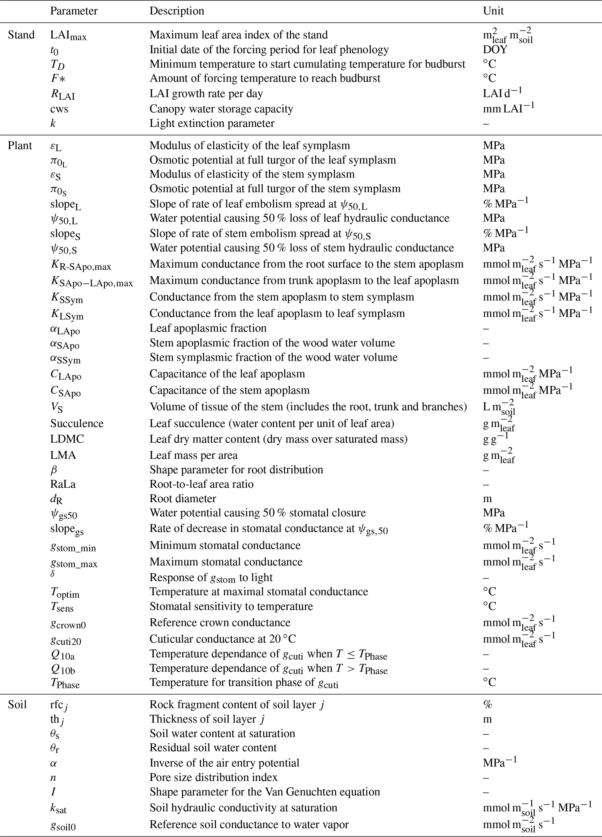
In addition to the core soil–plant hydraulic processes driving transpiration and plant water status (Q and ψ), SurEau-Ecos also includes an empirical module for leaf phenology that controls leaf area growth and decreases during senescence (described in Appendix A) and different modules to represent the stand water balance (interception, water transfers between soil layers and drainage; described in Ruffault et al. (2013). The list of input variables and their respective units is given in Table 1.
Temporal resolution varies according to each type of process (Fig. 1b). Phenology and stand water balances are computed at a daily time step. Soil–plant hydraulic processes (i.e., soil water uptake, transpiration and hydraulic redistribution) are computed at the finer time step (from 0.01 to 1800 s depending on the resolution scheme) and driven by hourly interpolated climate, which is derived from daily climate following (De Cáceres et al., 2021) (see Table B1 for the list of daily input weather variables). The three different numerical resolution schemes currently implemented in SurEau-Ecos are described in Sect. 2.6.
All variables and processes related to stand water balance processes (precipitation, interception, drainage) are expressed per unit of ground surface area, while plant hydraulic processes are expressed per unit of leaf surface area, in accordance with usual practices in each research field. This implies that initial water volumes of the soil and the plant (leaf and stem) are expressed per unit of soil area. Following this, leaf area index (LAI) permits the conversion of quantities from a soil area basis to a leaf area basis. If the parametrization is performed from individual tree dimensions or from forest inventories and allometries, an additional parameter is needed, the average plant foot print (aPFP, in m2), in order to scale individual plant dimensions on leaf or a soil area basis.
SurEau-Ecos was implemented in the R programming language (R Core Team, 2020). The following sections describe the equations and resolution of the model in more details.
2.2 Water balance in each compartment
2.2.1 Plant
The water balance of each of the four-plant compartments (leaf and stem symplasm and apoplasm, Fig. 1c) is determined according to the generic Eq. (4) and solved at each time step.
For the leaf apoplasm, the water balance equation is as follows.
The first term represents the change in water quantity related to the leaf apoplasmic capacitance (CLApo, mmol m MPa−1), which releases or absorbs water according to volume changes due to water potential changes (ψLApo, MPa). Contrary to symplasmic compartments, this term is very limited in the apoplasm because the xylem wall is inelastic. Note also that cavitation is not included in this capacitance. The second and third terms are the water exchanges between the leaf apoplasm and stem apoplasm and between the leaf apoplasm and leaf symplasm, respectively. ψSApo is the water potential of the stem apoplasm, ψLSym is the water potential of the leaf symplasm, KSApo−LApo (mmol m s−1 MPa−1) is the conductance from the stem apoplasm to leaf apoplasm and KLSym is the conductance of the leaf symplasm. This equation applies to the non-cavitated part of the xylem, which receives water from the cavitated part. This source is represented by the fourth term (mmol), which corresponds to the water release by the cavitated vessels towards the non-cavitated leaf apoplasm (Hölttä et al., 2009). This term is further described in Sect. 2.3.2, where we explain how it can be expressed as a function of ψLApo.
Water balance for the stem apoplasm is calculated as follows.
The first term represents the water flux related to the stem apoplasmic capacitance (CSApo) and water potential (ψSApo) changes during the time step. As with the leaf apoplasm, this term is in general very limited for the stem apoplasm. The second term represents the water exchange between the stem apoplasm and the three soil layers. For each soil layer j, is the conductance from the soil to the stem apoplasm and the soil water potential. The third and fourth terms represent flux to the leaf apoplasm and stem symplasm, respectively. ψSSym is the water potential of the stem symplasm and KSSym is the stem–symplasm conductance. The fifth term corresponds to the water released from cavitation to the non-cavitated stem apoplasm water reservoir.
Water balance for the leaf symplasm is as follows.
The first term represents the water flux related to CLSym and water potential changes of the leaf symplasm (ψLSym) during the time step. The second term is the exchange between leaf apoplasm leaf symplasm. The third and fourth terms represent the losses of water from the plant to the atmosphere through leaf stomatal transpiration (Estom) and cuticular leaf transpiration (). Note that with this formulation, leaf water losses from leaf transpiration remains lower bounded by even when stomata are fully closed (Estom=0).
Water balance for the stem symplasm is as follows.
The first term represents the water flux related to CSSym and water potential changes of the stem symplasm (ψSSym) during the time step. The second term is the flux to the stem apoplasm. The third term represents the losses of water from the plant to the atmosphere through minimum cortical transpiration (.
2.2.2 Soil
The water balance of each of the three soil layers (Fig. 1c) is determined according to the generic Eq. (5) and solved at each time step.
For the first soil layer, the following equation is required.
The first term (, mmol m) represents the change in soil water quantity between two consecutive time steps. The second term is the flux to the stem apoplasm. This flux is multiplied by LAI to convert water quantities from a leaf area basis to a soil area basis. pptsoil (mmol m) is the precipitation reaching the soil, D1→2 is the drainage (mmol m) of the first to the second layer, and Esoil (mmol m) is soil evaporation that occurs only from this layer.
Similarly, for the second layer the following equation is required.
For the third soil layer, the following equation is required.
Dd is the deep drainage (mmol m). For any layer, drainage occurs when the field capacity of the soil layer (θfc) is overpassed. Lateral water transfer processes and upward capillary transfers between layers are neglected. At the time step of the hydraulic model (δt) the water balance of each soil layer is treated according to the losses from transpiration and from evaporation (only for the first layer). Incoming fluxes from precipitation, drainage and transfers between soil layers are treated at a daily time step (Fig. 1b). Rainfall interception and drainage are treated as in SIERRA (Mouillot et al., 2001; Ruffault et al., 2013) and follow the design principles of several other water balance models (Rambal, 1993; De Cáceres et al., 2015; Granier et al., 1999).
2.3 Conductances and fluxes
2.3.1 Plant and soil conductances
The model includes four apoplasmic conductances (three root-to-stem and one stem-to-leaf conductance), two symplasmic conductances (one for the stem and one for the leaves) and three soil-to-root conductances (, one per soil layer j) (Fig. 1c). Symplasmic conductances of the leaves (KLSym) and stem (KSSym) drive the fluxes between the symplasmic and apoplasmic compartments. These conductances are set to a constant value throughout the simulation. Xylem (i.e., apoplasmic) conductances are composed of three root-to-stem conductances in parallel (, one per soil layer j) and one stem-to-leaf conductance (KSApo−LApo). These conductances can vary throughout the simulation from their initial value down to 0 according to the level of cavitation (expressed by the percent loss in conductance).
In practice, it is also useful to define the total plant conductance KPlant as follows:
The stem-to-leaf apoplasmic conductance (KSApo−LApo) is expressed as a function of the percent loss of conductance due to xylem embolism in the leaf:
where is the initial (maximum) root-to-leaf conductance and PLCL (%) is the percent loss of conductance. PLCL is proportional to the level of xylem embolism. It occurs when the water potential drops below the capacity of the leaf xylem to support negative water potential and is computed by using the sigmoidal function (Pammenter and Vander Willigen, 1998):
where P50,L (MPa) is the water potential causing 50 % loss of plant hydraulic conductance and slopeL (% MPa−1) is the slope of linear rate of embolism spread per unit of water potential drop at the inflection point P50,L.
The apoplasmic conductance from each root j to the stem apoplasm () is expressed as a function of the level of embolism computed at the node of the stem apoplasm:
where PLCS is computed as PLCL with the stem apoplasmic potential (ψSApo) and vulnerability curves parameters specific to the stem (slopeS and P50,S). is the maximal root-to-stem apoplasmic conductance of layer j. It is derived from fine-root area of the layer j such as
where KR−SApo is the total conductance of the root system. RAIj is the fine-root area of the layer j:
where RAI is the total fine-root area that is computed from the stand leaf area index and the root-to-leaf area ratio (RaLa) and ri the root fraction in each soil layer, which is determined according to the equation from Jackson et al. (1996):
where zh,j is the depth (m) from the soil surface to the interface between layers j and j+1, the factor of 100 converts from meters to centimeters and β is a species-dependent root distribution parameter (Jackson et al., 1996). Following this, the conductance between each soil layer j and the stem apoplasm () is determined as the result of two conductances in series, and the conductance from soil to root ():
The conductance of the soil to fine roots for each soil layer j is computed as follows:
with La and Lv the root length per soil area and soil volume for each soil layer, respectively, with both computed from soil depth and RAIj, whereas r is the radius of fine absorbing roots. ksat is the soil hydraulic conductivity at saturation, m is a parameter of shape from the van Genuchten equation and REW is the relative extractable water content computed as follows:
where θ is the relative water content (soil water content per unit of soil volume) changing dynamically with changes in absolute soil water reserve in the rooting zone, θs is the relative soil water content at saturation and θr is the relative soil water content at wilting point. θs and θr are parameters measured in the laboratory or derived from soil surveys with pedotransfer functions.
The total available water (TAW) for the plant can also be computed as the difference between the water quantity at field capacity (θfc) and the water quantity at θr summed over the three soil layers as follows:
where rfcj and thj are the rock fragment content (%) and thickness (m) of the soil layer j, respectively. TAW is not a parameter in SurEau-Ecos but is an integrative value resulting from the interaction between soil characteristics and rooting depth.
2.3.2 Cavitation
SurEau-Ecos also considers the capacitive effect of cavitation (Hölttä et al., 2009), i.e., the water released to the streamflow when cavitation occurs. The non-cavitated part of the xylem receives a water flux from the cavitated part, corresponding to in Eq. (6) (), and is then transferred to adjacent compartments. The amount of water corresponding to a new cavitation event is derived from the quantity of water in the apoplasm at saturation () and the temporal variations in PLCL as follows:
This flux is linearized in temporal variations in ψLApo in order to express this flux in the form of a Darcy's law to match the generic form of Eq. (2). For that purpose, we introduce an equivalent conductance () as follows:
where is the derivative of the PLC with respect to ψ, which is computed from the cavitation curve, and is the minimal value of potential ever reached over time, which controls the current cavitation level (). PLC′ is computed as follows:
Following the same approach, the flux derived from the stem when cavitation occurs is defined as follows:
2.4 Sources and sinks
2.4.1 Stomatal and cuticular plant transpiration
Plants lose water through stomatal transpiration (Estom), cuticular transpiration of the leaf () and cuticular transpiration of the stem (). Cuticular transpiration of the roots is considered to be negligible and is not taken into account. The total plant transpiration EPlant is decomposed as the sum of the leaf (EL) and wood transpiration ():
where Eleaf is computed as follows:
and is computed as follows:
where VPDL (MPa) is the vapor pressure deficit of the leaf, Patm is the atmospheric pressure (MPa), gstom is the stomatal conductance, is the cuticular conductance of the leaf, gbound is the conductance of the leaf boundary layer and gcrown is the conductance of the tree crown.
VPDL is a function of leaf temperature (TL). TL is computed at the leaf surface by solving the energy budget as in CPRM21. gbound and gcrown are computed following Jones (2013). gbound varies with leaf shape, size (dleaf) and wind speed; gcrown is a function of wind speed.
is a function of TL, which is based on a single or double Q10 equation depending on whether leaf temperature (TL) is above or below the transition phase temperature (TPhase) (Cochard, 2021):
if
if
where gstom is the stomatal conductance taking into account the dependence of gstom on light, temperature and CO2 concentration, as well as water status:
where gstom,max is the stomatal conductance without water stress and is determined as a function of light, temperature and CO2 concentration following Jarvis (1976). γ is a regulation factor that varies between 0 and 1 to represent stomatal closure according to ψLSym and an empirical sigmoid function depending on the potential at 50 % of stomatal closure (ψgs,50) and a shape parameter (slopegs) describing the rate of decrease in stomatal conductance per unit of water potential drop.
2.4.2 Soil evaporation
Esoil depends on the maximum soil conductance (gsoil0) and the REW of the first soil layer as follows:
2.5 Capacitances
As described in Sect. 2.1, the link between Q and ψ are not represented in the same way for the soil and plant compartments. The notion of capacitance is used for the plants, while water retention curves are used for the soil.
2.5.1 Plant compartments
The contribution of capacitance (C) to the plant compartment water balance is related to the saturated (or initial) water quantity (Q) in that compartment. Symplasmic and apoplasmic capacitances are not modeled in the same way, but both require the water volume at saturation (Qsat) of the considered reservoir. For the leaves, the volume of symplasmic and apoplasmic reservoirs at saturation ( and , respectively) are defined as follows:
with
where DM is the dry matter per unit of leaf area. The leaf dry matter content (LDMC), fraction of apoplasmic tissue in the leaves (αLApo) and leaf mass per area (LMA) are all input parameters.
The apoplasmic and symplasmic water quantities of the stem at saturation ( and , respectively) includes the volume of the roots, trunk and branches. They are computed based on the volume of the woody compartment and the water fraction of this volume as follows:
where VS is the volume of tissue of the stem compartment (including the root, trunk and branches), is the water molar mass, αWater is the proportion of water in this volume, and αSApo and αSSym are the apoplasmic and symplasmic fraction of this water volume, respectively.
Symplasmic reservoirs behave as variable plant capacitances related to the pressure volume curve, which corresponds to the water quantity changes in symplasmic cells (). Symplasmic conductances are functions of the and the temporal change in the symplasmic relative water content (RWC) (illustrated here for the leaf, but similar equations apply for the trunk):
with this formulation the capacitance of the leaf symplasm (CLSym) can be written as follows:
where RWC′ is the derivative of the RWC with respect to ψLSym, derived from pressure–volume curves (Tyree and Hammel, 1972; Bartlett et al., 2012).
We used the following formulation for RWC′ (see the justification below for the expression above ψtlp):
with
when .
In the above equation the formulation for ψLSym<ψtlp simply results from the fact that .
The case ψLSym≥ψtlp was obtained from basic manipulations of the derivation of the following form of the pressure–volume curve:
which with a derivative with respect to ψLSym becomes
and thus .
Apoplasmic capacitance is constant and is computed as the product between and the specific apoplasmic capacitance (CApo). Note that, given the very low elasticity of the xylem, this contribution is very weak.
2.5.2 Soil compartments
Capacitances for soil are not explicitly computed in SurEau-Ecos. Rather, soil water potentials for the different soil layers (ψsoil, MPa) are directly computed according to the van Genuchten parametric formulation (van Genuchten, 1980):
where m, n and α are empirical parameters describing the typical sigmoidal shape of the function and REW is the relative extractable water (see Eq. 21).
2.6 Numerical resolution
2.6.1 Plant compartments
The resolution of the plant hydraulic part of SurEau-Ecos is to solve the water balance for the four hydraulic compartments (i.e., nodes in Fig. 1c), whose equation are presented in Sect. 2.2.1. Three different numerical resolution schemes were implemented to solve water balances of plant compartments. For these three schemes, water potentials were discretized between two consecutive time steps, ψn and ψn+1, separated by δt. Thanks to cautious hypotheses, these equations were linearized at the first order in ψ, to lead to a four-equation linear system. Specifically, we neglected all variations of capacitances and conductances during a given time step (C≈Cn and K≈Kn), as these variations are expected to be marginal with respect to weather changes, stomatal regulation or water release by cavitation.
The simpler explicit scheme, also implemented in SurEau, assumes that water fluxes can be expressed from the current time step n (see Appendix B1 for details). From the generic water balance Eq. (4), it leads to
Rearranging this equation, the potential at the next time step ψn+1 can be simply computed as follows:
While the implementation of the explicit time integration scheme is undoubtedly the most straightforward numerical solution, it suffers from a well-known numerical constraint referred to as the CFL, which imposes very small time steps (δt) to avoid numerical instabilities:
This constraint implies that the smaller the C, the smaller the δt. An intuitive interpretation of this limitation is that the time step needs to be small enough to avoid water movements between non-adjacent cells. This constraint is particularly strong in plant xylem that is inelastic (i.e., C is very small) such that apoplasmic compartments cannot absorb water fluxes from their adjacent compartments when the time step is too large. This typically imposes δt to be smaller than 10 ms (CPRM21).
A common option to avoid these numerical instabilities is to use an implicit scheme, where fluxes are estimated from the values of ψ at time n+1 (ψn+1) as follows:
This numerical scheme is unconditionally stable, meaning that an increase in δt will not induce numerical instabilities but might induce a loss of numerical accuracy. One very important limitation of this scheme is that the equations of the different compartments now correspond to a system of four equations that are coupled. Such a system can be linearized (by pieces to account for thresholds such as cavitation) and solved. In general, it implies the inversion of the matrix of the linear system, but the resolution can also be done analytically when the equations are not too many, as it is the case with SurEau-Ecos (see details in Appendix B2).
An alternative scheme, based on a semi-implicit approach, has also been recently proposed to solve water balances in plant hydraulic models while overcoming the numerical instabilities associated with an explicit formulation (Xu et al., 2016; Tuzet et al., 2017; Li et al., 2021; De Kauwe et al., 2020). Although not usual in numerical resolution approaches, this scheme has been shown to have great performance and has led to convergence in simulations with time steps on the order of 10 min (Xu et al., 2016).
This approach consists of solving the differential equation of each compartment assuming that ψj and S remain constant (respectively equals to and Sn) as follows:
After linearization of the coefficient, this ordinary differential equation has the following solution:
Therefore, ψn+1 can be estimated by its value at u=δt:
which implies that
with
and
One can notice here that is the steady-state solution of the equation, typically valid when C=0 (fully elastic media).
In practice, this formulation is equivalent to the corresponding numerical scheme (provided that δt is very small):
This formulation allows for comparing this scheme to the explicit and implicit schemes proposed above. This scheme uses ψn+1 as a value for ψ (so that it remains stable) and as a value of ψj (so that the equations of the four compartments are decoupled) and can be seen as an intermediate between the explicit and the implicit scheme. For that reason, it will be referred to as semi-implicit (Appendix B3). In theory, the water fluxes computed from values of water potentials evaluated at different time steps should be less accurate than the implicit scheme, especially when water potential changes are fast. It is thus expected that simulations require a larger time step to converge than the implicit scheme.
For the three different numerical schemes, we assume that soil potentials were estimated at the current time step n (i.e., ) as in the explicit formulation (instead of n+1, as normally expected in an implicit scheme). This assumption is supported by the very small variations in soil potentials occurring during a single time and avoids the linearization of soil potential equations, which would have required unnecessary complex developments.
Source and sink fluxes Sn+½ are computed for the climate at the middle of the time step (mid-climate between the current and next time step at . For the implicit scheme, to account for the quick adjustment of stomatal regulation to climate variations, En+½ accounts for linear variations in water potential ψLSym over the time step, thanks to the derivative of transpiration function , also estimated for the mid-climate, but the current regulation of is as follows:
2.6.2 Soil compartments
Soil water balance in SurEau-Ecos is solved for each soil layer (Sect. 2.2.2) following a simple explicit scheme assuming that water fluxes can be expressed from the current time step n. From the generic soil water balance Eq. (5), it leads to
In this section, we explore the benefits and limitations of the three numerical schemes implemented in SurEau-Ecos to solve water fluxes, namely an explicit, semi-implicit and implicit scheme. As mentioned above, the minimal time step required for accurate simulations is determined by computational limitations that depend on the chosen scheme. First, unlike the implicit and semi-implicit scheme, the explicit scheme is limited by the CFL, which causes numerical instabilities. We explored how much computation time can be gained by using implicit or semi-implicit schemes compared to the explicit scheme. In addition, in the case of the implicit and semi-implicit scheme, reducing the temporal resolution (i.e., increasing the time step) can also limit the accuracy of the simulation. The magnitude of corresponding errors then depends on the physiological processes at play in the plant and on the precision of the numerical scheme. We also assessed the sensitivity of model outputs to the temporal resolution (time step δt) for the implicit and semi-implicit schemes.
For these simulations, all inputs were set identical to those used in the section dedicated to the evaluation of SurEau-Ecos (see Sect. 4). Daily weather was kept constant, without precipitation, and simulations were run until total hydraulic failure of the plant. To compare the explicit scheme with the two other schemes, we made two slight simplifications to the model. First, we neglected the cavitation term in Eqs. (6) and (7). Indeed, the explicit numerical scheme of SurEau-Ecos cannot account for the flux term associated with water released by cavitation. This is due to the direct dependence of and on δt (Sect. 2.3.2) that prevents the CLF from being satisfied at any time step. Second, the values for stem and leaf of apoplasmic capacitances (CSApo and CLApo) were increased (from about to 10 mmol m2 MPa) to decrease computational costs and ease the comparison between the numerical schemes. The CFL constraint imposed very small time steps (on the order of s) with the original values of plant apoplasmic capacitance, which caused unaffordable computation times under most CPUs. Preliminary analyses showed that the impact of CSApo and CLApo were negligible on simulation results for values up to 50–100 mmol m2 MPa.
When using the implicit or semi-implicit schemes with a relatively small time steps (δt=10 s) our results show that these schemes yielded identical plant dynamics to those obtained with the explicit mode (Fig. 2). However, the gains in computation time were considerable. Computation time was divided by about 10 for the implicit and semi-implicit scheme compared to the explicit scheme. This is because δt had to be set to 1 s for the explicit theme because of the CFL. Any attempt to set a δt above this 1 s threshold caused (as expected by the CFL) critical numerical instabilities (Fig. B1). Since some modifications to the model had to be performed for this comparison, the differences in computation times were solely indicative and were reported to illustrate the benefits of the semi-implicit and implicit schemes compared to the explicit scheme. Our results showed that the semi-implicit scheme was less accurate than the implicit scheme. Smaller time steps were required for the convergence of the model. Numerical explorations show that the semi-implicit scheme requires time steps on the order of 1 min (which is slightly slower than described in Xu et al. , 2016, which stated that 10 min was enough), whereas the time step can be generally larger than 30 min with the implicit scheme (Figs. B2 and B3).
Table 2Comparison of computation times between the three resolution schemes implemented in SurEau-Ecos.
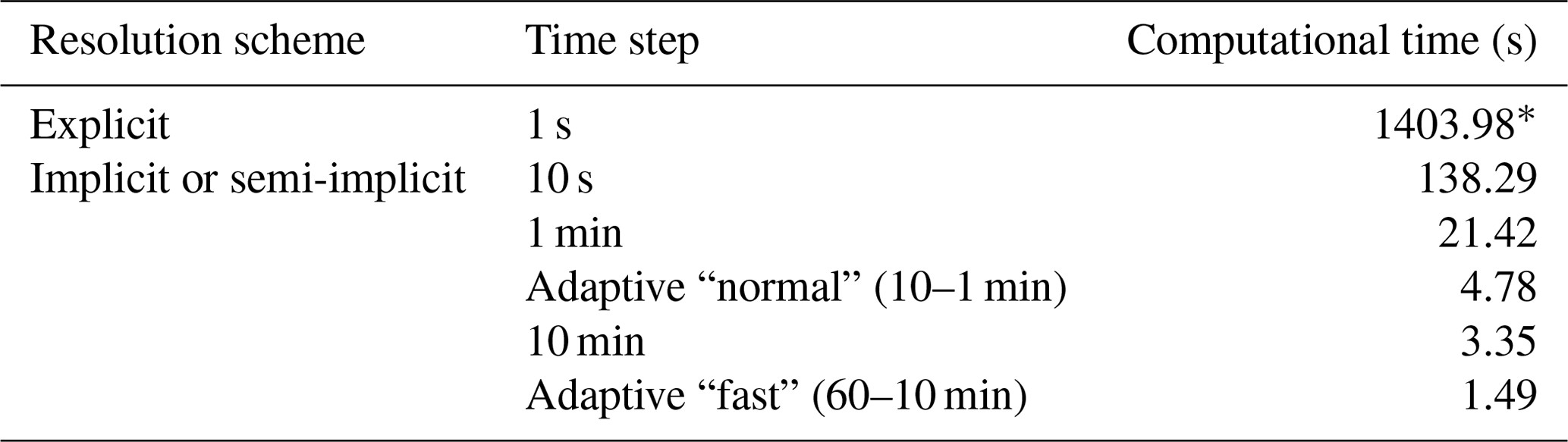
* This computational time is for indicative purposes only as several changes had to be made to the model to run it with the explicit scheme (see details in main text).
For the implicit and semi-implicit schemes, two adaptive time steps were further implemented to reduce computation times. This improvement was based upon the assumption that smaller time steps were only required when changes in two critical processes, stomatal regulation and cavitation, were the highest. In a “normal” mode, the base time step is at 10 min but is automatically and gradually refined up to 1 min in periods of intense regulation changes, based on a criterion aimed at preventing variation in stomatal regulation and cavitation of more than 1 % between two consecutive time steps. In a “fast” mode, the base time step is at 1 h and refined up to 10 min. The implementation of adaptive time steps allowed for further increasing this gain in computing time (Table 2) without affecting plant dynamics.
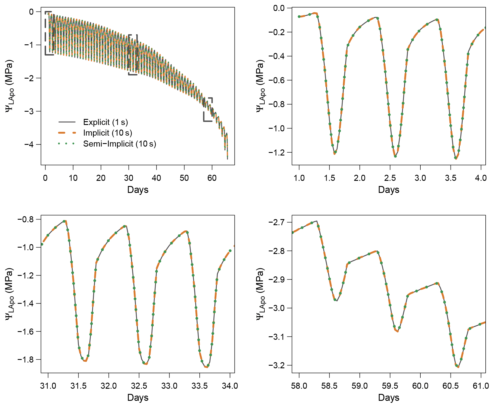
Figure 2Comparison of the three numerical schemes implemented in SurEau-Ecos to solve water balances. Computation times for each scheme are given in Table 2.
Due to the reduction of plant compartments, SurEau-Ecos requires fewer parameters than SurEau. However, the parametrization of plant hydraulics models can be problematic, especially for large-scale applications (i.e., for many species and stands). In order to facilitate the parametrization of SurEau-Ecos, we provided a table where we listed the most important parameters and where to find relevant datasets (Table 3). We also proposed some procedures to estimate the value of the parameters not directly available in current databases. We distinguished four different types of parameters: (i) the species-specific parameters, (ii) the plant (or stand) morphological parameters, (iii) the soil parameters and (iv) the parameters linked to hydraulic conductance.
Species-specific parameters (leaf, stomatal and hydraulic traits) can be derived from direct ecophysiological measurements or traits databases. This includes the parameters related to stomatal conductance, now available in several databases (Klein, 2014; Lin et al., 2015), and parameters of the p−v curves and vulnerability curves to cavitation both for the leaves and stems. The p−v curves are generally available for leaves (Bartlett et al., 2016), but very few data are available for the stem (but see Tyree and Yang, 1990; Meinzer et al., 2008). Until the release of additional datasets for these traits, we recommend to use the same value for the leaf and the stem symplasm. Vulnerability curves to cavitation are increasingly available at the branch and leaf level. In cases where it would be difficult to find the data for either the stem or the leaves, some hypotheses regarding the level of segmentation can be made. However, for vulnerability curves to cavitation, we recommend paying attention to the method that has been used to build the curves, as many artifacts are known to influence these values depending on the tree species (Sergent et al., 2020). Cuticular conductance at a reference temperature (gcuti20) and its dependence on temperature (Q10a, Q10b, and TPhase) are increasingly recognized as a key trait for survival time during drought (Duursma et al., 2019) and heat waves (Cochard, 2021). gcuti20 is increasingly available in species trait databases, but the parameters driving gcuti dependence to temperature are far less measured (Riederer and Schreiber, 2001). Recent methodological innovations should allow a greater acquisition of this trait (see Billon et al., 2020).
The plant (or stand) morphological parameters that determine the overall leaf area index (LAI) and the plant internal water stores can be derived from forest inventory and species-specific allometries. LAI can also be derived from vegetation remote sensing data.
The soil parameters determine the total soil available water for plant (TAW, see equation 23), which depends on the volume of soil explored by roots on the one hand (i.e., a function rock fragment content and rooting depth) and the water retention curve on the other hand (i.e., the relationship between water potential with soil water content). Such parameters can primarily be derived from soil databases. Note, however, that such databases generally provide only pedo-physical information (textures, organic matter content, rock fragment, depth) so that it will be needed to apply pedotransfer function to compute the parameters (Tóth et al., 2017). Pedotransfer function can also be used to compute the soil hydraulic conductance (KSat), although KSat global databases are also available (Gupta et al., 2021).
Finally, the hydraulic conductance of the soil-to-leaf pathway and its repartition within the plant is rarely available (Mencuccini et al., 2019). The easiest way to obtain some values for these parameters is to compute the total maximal plant hydraulic conductance by using flux data (derived from sap flow, leaf gas exchange or remote sensing) and in situ water potential data (Mencuccini et al., 2019). The distribution between compartment can then be done by using average hydraulic architecture maps (Tyree and Ewers, 1991; Cruiziat et al., 2002). Alternatively, this can be computed from the elementary conductivity of plant organs taken from databases and plants sizes derived from inventory (De Cáceres et al., 2021).
Table 3Parametrization of SurEau-Ecos. Note that p–v stands for pressure–volume curve.
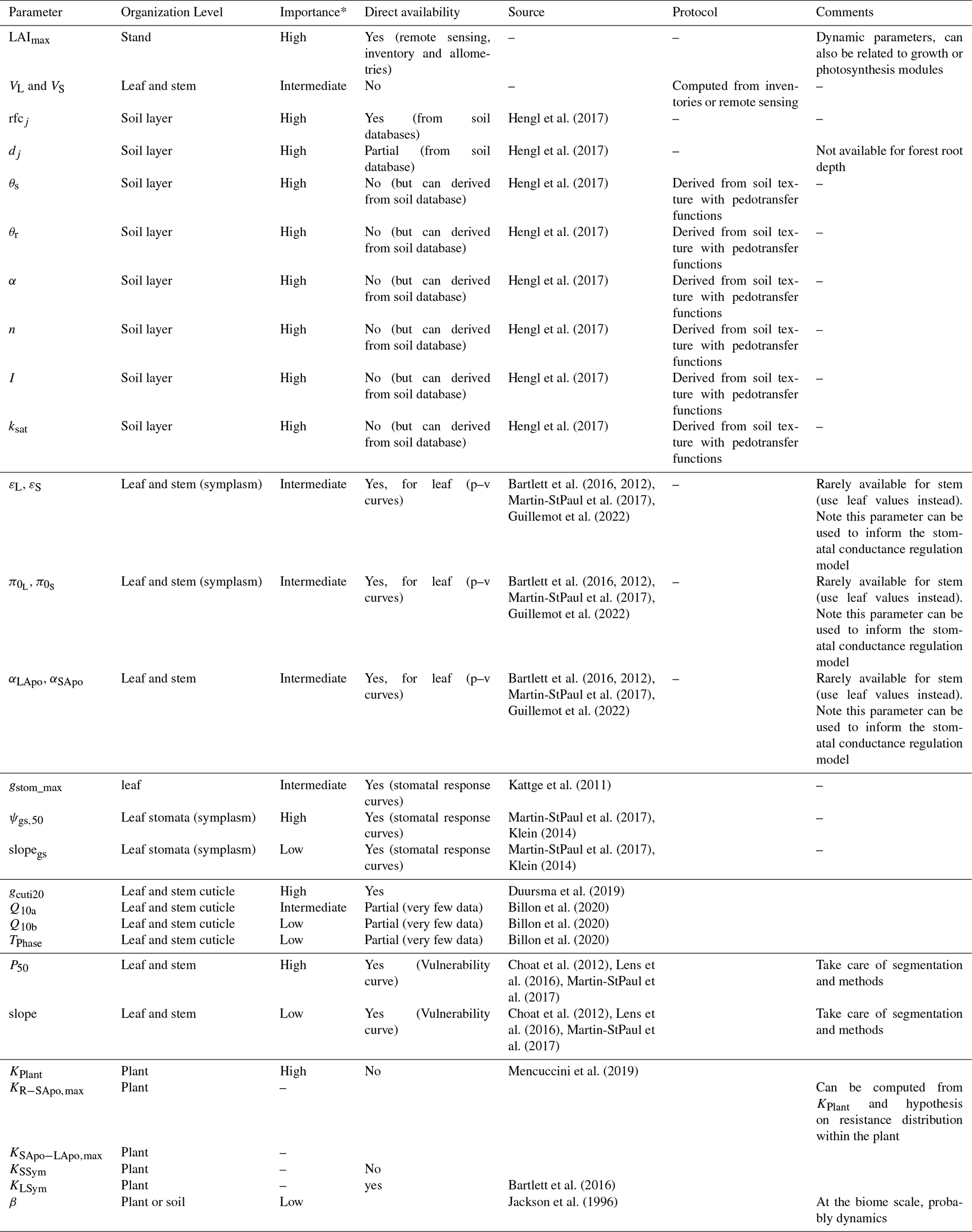
* The importance of each parameter was determined from preliminary analyses and the results of sensitivity analyses (Sect. 6) for reference only as it might vary depending on the species or the climate conditions. The description and unit of each parameter is given in Table 1.
SurEau-Ecos relies on the same biological and physical principles of SurEau (CPRM21). The soil–plant–atmosphere system is segmented and described as compartments linked together and exchanging water fluxes according to the gradients of water potential and hydraulic conductances. However, significant disparities between the implementation, parametrization and resolution of water fluxes between the two models led to some major differences in plant architecture and representation of water fluxes. It was therefore essential to confirm that both models provide comparable dynamics of the main state variables under similar conditions. This comparison of model outputs also consists at as an indirect evaluation effort of SurEau-Ecos since SurEau has been evaluated against field data (see details in CPRM21).
We identified three major differences in plant architecture and representation of hydraulic processes within the models. First, plant architecture is simpler in SurEau-Ecos than in SurEau. SurEau-Ecos represents the plant as two leaf cells (leaf apoplasm and leaf symplasm) and two stem compartments that include the woody volume of branches, trunk and roots. In contrast, SurEau offers a detailed plant organ discretization (including roots, trunk, branches, leaves and buds). Second, while both models represent the belowground stems by three roots in parallel, the resistance to water flow linked to the root endoderm (a symplasmic root resistance) is not explicitly included in SurEau-Ecos contrary to SurEau. Instead, only one resistance per root, from the root entry to the stem, is accounted to mimic all possible resistance (root symplasm and apoplasm). Finally, in SurEau-Ecos, all leaf level fluxes to the atmosphere – i.e., the stomatal and the cuticular fluxes – pass through the symplasm, whereas in SurEau stomatal fluxes pass through the apoplasm and cuticular fluxes.
To compare model outputs, we performed an equivalent parameterization of the two models (see details in Fig. B4) and ran simulations until total hydraulic failure of the plant. We started the comparison with a typical plant fully described in CPRM21 whose parameters are given for each organ in Table B2. We then aggregated the values of SurEau parameters to match the following input parameters of SurEau-Ecos: water quantities of the leaf and stem compartments (, , and ), the symplasmic conductance of the stem (KSSym), the apoplasmic root-to-stem conductance (KR−SApo) and the apoplasmic stem-to-leaf conductance (KSApo−LApo). We also set the cuticular conductance of non-leaf organs to 0 in both models. All other submodels, parameters and environmental forcing (weather and soil) were also set equal, including stomatal, boundary layer and crown conductance, linear approximation for the leaf energy balance, soil parameters, and hourly climatic inputs. This ensured that any divergence between models could only come from either the numerical scheme or plant hydraulic architecture.
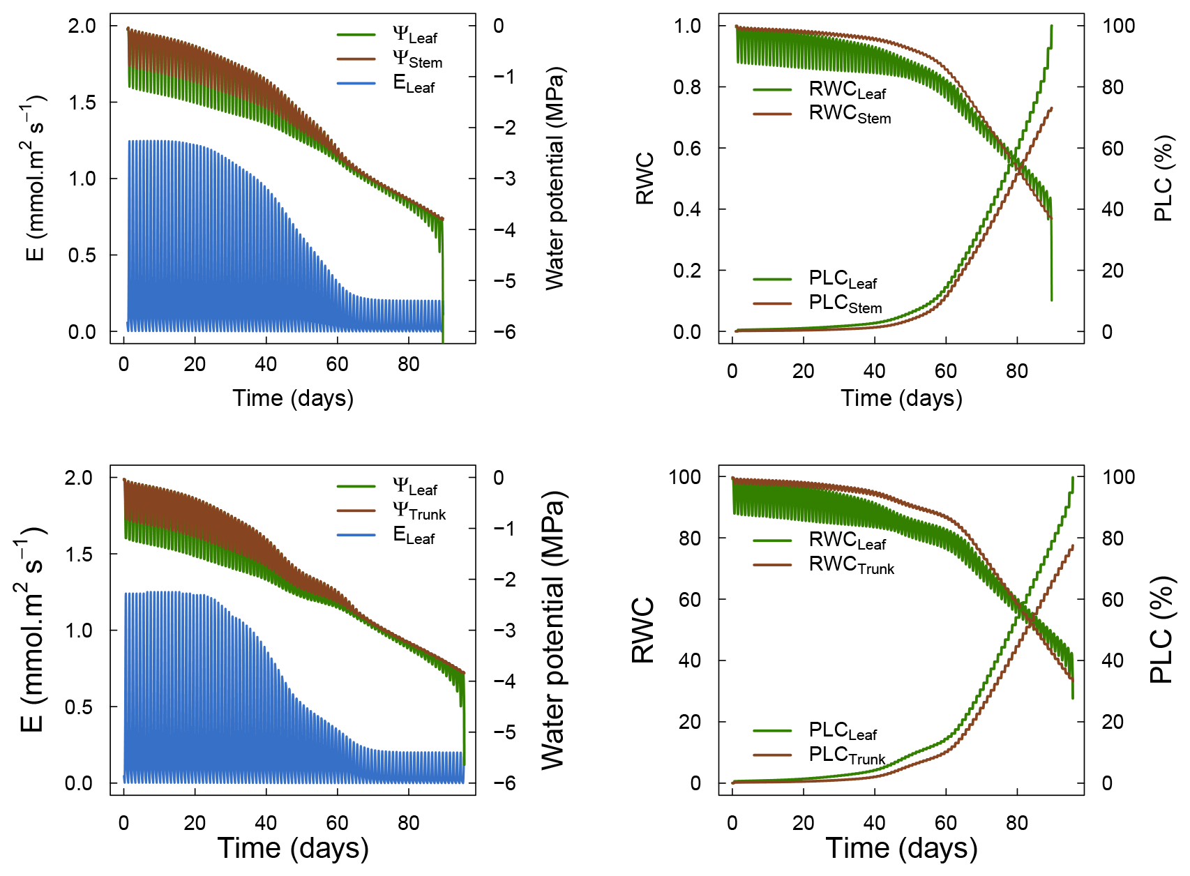
Figure 3 shows the dynamics of water potentials, leaf transpiration and percent loss of conductance obtained when simulations were run from a wet soil profile until hydraulic failure is reached. Note that for this comparison the output of the trunk in SurEau was compared to the stem in SurEau-Ecos. For both models, at the beginning of the simulations when the soil was wet, leaf and stem water potentials followed the hourly variations in meteorological conditions, thereby reflecting the response of stomata to light and response of plant transpiration to gstom and VPD. As the soil reservoir emptied, stomata progressively closed according to the intensity of foliar water potential. After about 65 d for both models, the stomata permanently closed and transpiration was limited to cuticular losses that gradually accentuated the drought stress of the plant (decreased plant water potentials). Simultaneously, cavitation increased in the different organs, inducing water release from the apoplasm which partly dampened the decrease in plant water potentials. These results show that SurEau-Ecos and SurEau yielded very similar results when parameterized in such a way that plant organs had similar conductances and water reservoirs.
Despite similar dynamics, we also identified some differences in infra-daily water potentials between the two models. As a result, the time to leaf hydraulic failure was underestimated by 3 d (out of 90 d) in SurEau-Ecos compared to SurEau. These slight differences can be linked to the presence of the higher number of compartments in SurEau that increase the seasonal dampening effect of water potential compared to SurEau-Ecos where a lower number of compartments are represented. Notably, we observed some differences between the short-term (infra-daily) variations in the water potential dynamics of the trunk symplasmic compartment of SurEau and the stem compartment of SurEau-Ecos (including the volume of roots, trunk and branches; see Table B2). The daily magnitude of the fluctuation in SurEau-Ecos appeared more dampened (Figs. 3, B5 and B6). The most plausible explanation for this difference is that the volume of the stem compartment in SurEau-Ecos is greater than the volume of the trunk compartment in SurEau. This is likely to lead to greater water discharge and lower water potential fluctuations in SurEau-Ecos (Fig. B6). Ongoing developments of a modular version of SurEau within the Capsis modeling platform (Dufour-Kowalski et al., 2012) will allow us to more deeply evaluate the effects of plant hydraulic architecture on the dynamics of plant desiccation.
6.1 Model sensitivity to input parameters
We carried out a variance-based sensitivity analysis to gain insights into the species traits that influence plant water dynamics in SurEau-Ecos and explore the main drivers of tree response to extreme drought. Variance-based approaches can measure sensitivity across the whole input space (i.e., it is a global method) and quantify the effect of interactions that can be unnoticed on a local sensitivity analysis approach (i.e., when moving one parameter at a time). Here, we used the Sobol's sensitivity analysis method (Sobol, 2001) and reported “total order indices” that quantify the contribution of each parameter to the variance of the model output.
Two different physiological phases control the dynamics of plant desiccation under extreme drought, according to whether ψLSym is above or below the point of stomatal closure (Fig. 1a). Three time-based metrics were therefore considered to explore the sensitivity of plant desiccation to input parameters: (i) the time to hydraulic failure, (ii) the time to stomatal closure, and (iii) the survival time, defined as the time difference between hydraulic failure and stomatal closure (see an illustration in Fig. 4). We performed a sensitivity analysis for three different tree species with contrasting ecology and which exhibited various combinations of input parameters (Table 4). For each parameter, we randomly sampled a value within a range of ±20 % of the observed value. Starting from a wet soil, and without further precipitation, we ran simulations until hydraulic failure of the plant, defined as the moment when leaves reach 99 % loss of hydraulic conductivity ( %). This threshold guarantees that plant water pools were almost empty and that no other water reservoirs are available for the plant. The water content of plant tissues is probably a better indicator of plant mortality than the percent loss of conductivity (Martinez-Vilalta et al., 2019; Mantova et al., 2021). However, an accurate prediction of moisture content would require the integration of carbon metabolism (Martinez-Vilalta et al., 2019) that is currently not implemented in SurEau-Ecos. Daily climate inputs were set constant according to the simulations shown in Sect. 4. In total, we ran 700 000 simulations in the sensitivity experiment.
We based our selection of parameters used in the sensitivity analysis on the results from preliminary analyses and from the findings by CPRM21. To ease the interpretation of the results, we grouped the parameters according to several families, representing different processes: “water use” (LAImax, KPlant, TAW and gstom,max), “regulation” (ψgs,50), “water leaks” (gcuti20, Q10a), “safety” (P50) and “plant internal stores” (VS) (see definition in Table 1). The total available water (TAW) for the plant is not an input parameter in SurEau-Ecos, but it is an integrative index resulting from the interaction between soil characteristics and rooting depth. TAW is determined as the difference between the water quantity at field capacity and the water quantify at residual water content cumulated over the three soil layers. To make TAW vary in simulations without affecting soil physical properties, we adjusted rooting depth to match the targeted TAW.
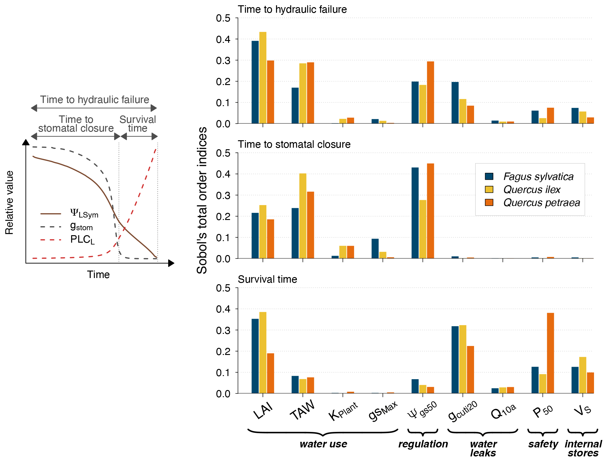
Figure 4Global sensitivity analysis of plant desiccation dynamics to the main hydraulic traits and stand parameters in SurEau-Ecos, shown for three different tree species with contrasting ecology and which exhibited various combinations of input parameters. We explored the sensitivity of three physiological time-based metrics to input parameters: time to stomatal closure, time to hydraulic failure and survival time. These three metrics describe the two different physiological phases controlling the dynamics of plant desiccation under extreme drought, according to whether ψLSym is above or below the point of stomatal closure (Fig. 1a). All traits varied ±20 % around their original value. TAW is the total available water for the plant.
Our results showed that a few parameters explained most of the variability in the response of trees to extreme drought (Fig. 4), although their importance largely depended on the physiological phase under study. The parameters related to “water use” (LAImax, TAW and KPlant) and “regulation” (ψgs50) mainly explained the variance in time to stomatal closure, i.e., the first physiological phase. It suggests that, in this phase, interactions between how much water is available in the soil (TAW) and how fast plant transpiration will empty that reservoir (LAImax, ψgs,50 and KPlant) determine the time to stomatal closure. The surprisingly relative low influence of gstom,max on the time to stomatal closure could be explained by the fact that, with that set of parameters and environmental conditions, KPlant has a more limiting impact on plant transpiration than gstom,max. In the second phase (after stomatal closure), survival time was mostly driven by parameters related “water use” (LAI, P50), “water leaks” (gcuti20), “safety” (P50) and “plant internal stores” (VS). In that phase, the importance of TAW and ψgs,50 decreased to the benefit of traits related to the rate of water losses through cuticular transpiration (gcuti20 and Q10a); the volume of water reservoirs in the root, trunk, and branches (VS); and plant resistance to cavitation (P50). When both phases were considered jointly, we observed that the variability in the time to hydraulic failure was mainly associated with stand parameters (LAI and TAW) and to a lesser extent with ψgs,50 and gcuti20.
We also observed that the patterns described here above were almost identical regardless of the vegetation type under study. In particular, the parameters controlling “time to hydraulic failure” and “survival time” were similar among the three studied vegetation types, suggesting a similarity of plant adaptation strategies to avoid hydraulic failure in a changing climate. The one exception to this pattern is the importance of varying plant resistance to cavitation (P50) in survival time. The influence of P50 ranged from low for Quercus ilex (about 0.05) to very important for Quercus petraea (about 0.37). This observation suggests that less drought-resistant species (with higher P50) receive a more direct benefit when lowering their P50 to increase their survival time than drought-resistant species (with lower P50). This might be due to the nonlinear response of water potential to soil and plant water content, which implies that the rate of change of plant water potential increases as soil and plant water content decreases.
Our results shed some light on our understanding of plant functioning under extreme drought. We highlighted the prominent role of stand traits, namely LAImax, TAW and ψgs,50, in determining the time needed to reach stomatal closure. In contrast, physiological variables, namely gcuti20, Q10a, VS and ψ50,L, played a more important role in determining “survival time”. Two improvements to the present analyses may strengthen these findings. First, numerous correlations exist between those traits, reflecting trade-offs and plant functioning strategies (Christoffersen et al., 2016; Martin-StPaul et al., 2017) that we did not take into account. Similarly, it has been shown that LAImax and TAW covary because trees with a higher amount of available water tend to develop a higher leaf surface value (Hoff and Rambal, 2003). Second, the relative importance of input parameters is likely to be influenced by climate. For instance, we would expect the influence of gmin20, Q10a and Q10b on survival time to increase when temperature increases, following previous results showing the vulnerability of trees during heat waves (Cochard, 2021). Integrating these potential improvements in future simulations may further help to elucidate the specific spatial and temporal patterns of drought-induced mortality (Meir et al., 2015).
6.2 Model sensitivity to the inclusion of symplasmic and apoplasmic capacitances
Whether or not plant hydraulic capacitances are explicitly taken into account is one of the key distinctions between current large-scale plant hydraulic models. Some models represent trees as single- or multiple-resistance organisms (e.g., Kennedy et al., 2019), while others like SurEau and SurEau-Ecos also include one or several hydraulic capacitances. SurEau and SurEau-Ecos describe the soil–plant–atmosphere system as a network of resistances and capacitances while introducing a novel distinction between the symplasmic and apoplasmic capacitances. This approach is beneficial for model parametrization and to derive values such as water content, as has already been discussed in Sect. 2. However, the role and importance of both the symplasmic and apoplasmic capacitances for plant survival and water dynamics have not yet been studied.
To further understand the role hydraulic capacitances on plant water dynamics, we conducted sensitivity experiments were capacitances were successively set to zero: first apoplasmic capacitance (leaf and stem), then symplasmic capacitance (leaf and stem), and finally both apoplasmic and symplasmic capacitances. These simulations applied the same experiment settings as the model comparison experiment (see Sect. 4), i.e., similar plant parameters, soil and climate conditions.
Figure 5 shows the results of the simulations of the sensitivity experiment. Overall, hydraulic capacitances induced significant differences in both the dynamics of plant water potentials and the time to hydraulic failure. More specifically, we observed that symplasmic capacitance can buffer short-term variations in plant water potentials and therefore induced fewer negative values at midday. Apoplasmic capacitances played a major role in both delaying the time to hydraulic failure and buffering daily variations in plant water potentials by providing water when cavitation occurs. The importance of this effect increases with decreasing water potentials (increasing drought). Our results therefore suggest that the representation of plant water storage greatly affects the simulations of plant water dynamics. Further studies aimed at measuring plant water content will help to validate and affine the role of plant water storage for tree response to extreme drought.

Figure 5Model sensitivity to the inclusion of symplasmic and apoplasmic capacitances in SurEau-Ecos.
Table 4Main parameter values used in the model simulations whose results are shown in Figs. 4 and 5. Parameters derived from pressure–volume curves and PLC curves were set equal for the leaf and stem (, ). The description and unit of each parameter is given in Table 1.

In this section, we aimed to illustrate the potentialities offered by SurEau-Ecos for improving our understanding of forest response to drought. We explored whether the probability of plant hydraulic failure simulated by SurEau-Ecos was related to the distribution of two tree species at their southern distribution margin, and we then used this information to identify future areas at risk of drought-induced tree mortality. Specifically, we hypothesized that hydraulic failure was a significant constraint to tree distribution at the regional level.
We quantified the probability of hydraulic failure over France (544 000 km2) for two different species chosen for their contrasted functioning strategies: an evergreen Mediterranean oak (Quercus ilex) and a temperate deciduous European beech (Fagus sylvatica) (see main parameters in Table 3). Quercus ilex is a drought-resistant species with low LAI, P50, and deep root systems to extract water from cracks in the bedrock during drought. In contrast, Fagus sylvatica is characterized by a higher vulnerability to drought (higher P50) and higher LAI values. As in Sect. 5, we defined hydraulic failure as the point when leaves reach 99 % loss of hydraulic conductivity (PLCL≥99 %). For each period investigated, we reported the probability of hydraulic failure as the frequency of years during which PLCL≥99 %.
We ran simulations for present (1991–2020) and future (2071–2100) periods at an 8 km2 resolution over France for both species. Climate data for the present period (1970–2020) were extracted from the SAFRAN climate reanalysis database (Vidal et al., 2010), which covers France at an 8 km2 resolution. Projections of climate variables for the future climate period (2071–2100) were obtained from a climate simulation program involved in the fifth phase of the Coupled Model Intercomparison Project (CMIP5) and produced as part of the EURO-CORDEX initiative (Kotlarski et al., 2014). One single global circulation model–regional climate model (GCM–RCM) couple was extracted for these analyses (i.e., MPI-ESM-REMO2009), which was chosen because of its averaged climate trajectory over France when compared to an ensemble of GCM–RCM couples (Fargeon et al., 2020; Ruffault et al., 2020). Data were extracted at a 0.44∘ spatial resolution for the historical (1990–2005) and future (2006–2099) periods. Model outputs were bias-corrected and downscaled at the 8 km2 resolution using a quantile–quantile correction approach (Ruffault et al., 2014).
To apply the model at the landscape scale, we made several simplifying assumptions. First, we assumed that each 8 km2 grid cell was covered by trees of the same species and that LAI was set to a constant value representative of observed values for the considered species (Table 3). Second, soil characteristics were also set constant over the territory. Both assumptions are unrealistic because stand characteristics vary at the local scale and have a primordial role in the probability of hydraulic failure (Sect. 5). However, as we aimed to assess the regional (rather than the local) vulnerability of tree species to changes in climate, we did not expect this to be a main limitation, provided that the results of these simulations be interpreted accordingly to these assumptions. To assess whether the probability of hydraulic failure was a good proxy of the current southern range of tree species distribution, we compared the results of our simulations with presence and absence data for each species. Tree species data were extracted from the national forest inventory database (available at http://www.ifn.fr, last access: 12 May 2022) and aggregated to obtain presence–absence on the 8 km studied grid following Cheaib et al. (2012).
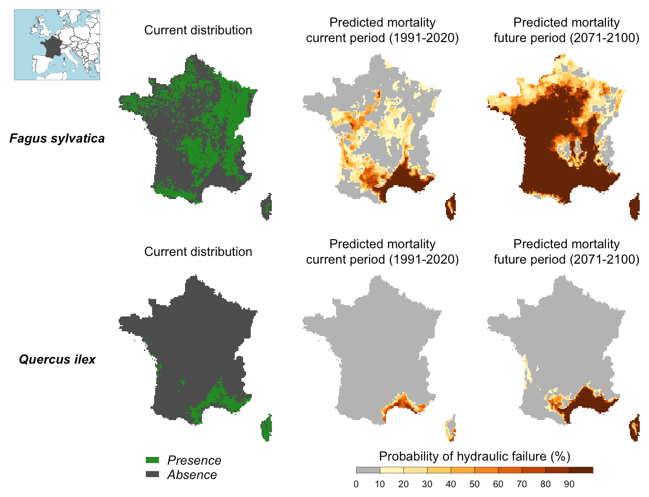
Figure 6Probability of hydraulic failure (%) over the past (1991–2020) and future (2017–2100) period for two tree species in France simulated with SurEau-Ecos. The current distribution is shown for comparison with the simulated risk of hydraulic failure.
Maps of probability of hydraulic failure (probability of reaching PLCL≥99 %) are shown in Fig. 6. We observed contrasting regional patterns according to the species under study. We observed a higher probability of mortality in southeastern France for both species, but the probability of hydraulic failure was higher for the European beech than for the holm oak. In the rest of the country, the probability of hydraulic failure was almost 0 for the holm oak. In contrast, we observed probabilities up to 50 % for the European beech in the western part and middle of the country, where the climate is temperate. When comparing these results with the maps of current species distribution, we observed a reasonable degree of spatial agreement between our simulations and presence/absence data. European beech was predominantly present in areas where our simulations indicated a probability of drought-induced mortality equal to 0 %. However, we could not interpret the results for the holm oak in the same way since the current distribution of this species indicates that the southern climate margin is not reached in the present climate. In the parts of the country where summer drought is less intense, several other factors might explain why Quercus ilex is currently not observed, including competition from more productive species, cold resistance or even forest management policies.
Our projections for the end of the century showed a future increase in the areas characterized by a high risk of hydraulic failure over France. For Fagus sylvatica, the areas characterized by a high risk of hydraulic failure will extend towards the northeast and west of the country (i.e., over the major part of the territory). For Quercus ilex, our simulations indicated that the probability of hydraulic failure should significantly increase in southeastern France, where this species is currently widespread.
Altogether, these results indicate that future climate conditions might overcome the capacity of the two studied tree species to face drought over France, which might increase the likelihood of tree mortality and wildfires in the future. Adding information about the LAI and soil physical properties might further refine our simulation results. LAI can be estimated from remote sensing indices (see for instance (De Kauwe et al., 2020). However, TAW estimations are more problematic because information about root depth is rarely available (Ruffault et al., 2013; Venturas et al., 2020).
SurEau-Ecos can already be applied as a standalone model to understand plant water dynamics and can be used in a wide of research applications, from stand-scale estimations of water fluxes to regional predictions of drought-induced mortality (see Sect. 7). In addition, the specific distinction between the symplasmic and apoplasmic compartments implemented in SurEau-Ecos provides a solid foundation for predicting and monitoring water storage in the plant, a key factor in ecosystem disturbances such as mortality (Martinez-Vilalta et al., 2019) and wildfires (Ruffault et al., 2018b; Pimont et al., 2019).
The development of several supplementary key processes also warrants future consideration to extend the range of research questions and applications that SurEau-Ecos would be able to address. First, SurEau-Ecos currently simulates plant water dynamics for a single tree species for a homogeneous forest stand, and it therefore neglects the effects of species interactions on tree response to drought. This would, however, require us to affine the current representation of water competition between trees and microclimatic effects. Such developments would not only provide a mechanistic basis for multi-species modeling but could also help us to better understand the processes driving heterogenous mortality in the canopy and integrate the effects of forest management on stand structure microclimatic conditions. Another important limitation of SurEau-Ecos is that it does not simulate the processes related to photosynthesis, respiration, growth and carbon allocation. Future developments will aim at integrating SurEau-Ecos with other forest models that are designed to represent the carbon cycle and vegetation dynamics, including the forest growth models CASTANEA (Dufrêne et al., 2005) and GO+ (Moreaux et al., 2020), as well as the gap model ForCEEPS (Morin et al., 2021) under the Capsis platform (Dufour-Kowalski et al., 2012). These future research projects and developments will also be an opportunity to further evaluate the feedbacks between carbon balance, growth metabolism and hydraulic properties, including the impacts of post-drought growth on the recovery of hydraulic properties and therefore on tree vulnerability to water stress in the long run (Arend et al., 2022).
Drought is arguably one of the most important natural disturbances threatening forest ecosystems in a number of regions worldwide (Allen et al., 2015). The challenges facing our understanding of the role of plant hydraulics in vegetation dynamics are numerous (McDowell et al., 2019), with one being the ability of current vegetation models, including those based on plant hydraulics, to predict plant desiccation dynamics at regional scales (Venturas et al., 2020; De Kauwe et al., 2020; Rowland et al., 2021; Trugman et al., 2021). Here, we presented SurEau-Ecos, a new plant hydraulic SPA model aimed at predicting plant water status and drought-induced mortality at scales from stand to region. SurEau-Ecos was designed to simulate the plant water status of the different plant's compartments, while at the same time balancing for the needs of input parameters and computational requirements. SurEau-Ecos simulates key mechanisms associated with plant desiccation during drought and heat waves, including the dynamics of plant's water status beyond the point of stomatal closure via residual transpiration flow, plant cavitation and the solicitation of plants' water reservoirs. We showed that SurEau-Ecos was able to provide accurate estimations of plant water status dynamics compared to the SurEau model, despite the latter representing plant hydraulics mechanisms in more detail. This confirms that, for large-scale applications, the changes we implemented in SurEau-Ecos largely outweigh a potential loss of accuracy associated with the simplification of plant architecture and hydraulic processes. SurEau-Ecos provides the capability for us to better understand the role of plant hydraulics in vegetation dynamics under climate-change conditions characterized by increased drought frequency.
Leaf area index (LAI) of the stand is updated daily. Species can have either evergreen or winter deciduous phenology. Evergreen species are assumed to maintain a constant LAI throughout the year. LAI values of deciduous plants are adjusted as a function of leaf phenology (∅) and the maximum of the stand (LAImax) as follows:
∅ is set to 0 until budburst occurs. Budburst is assumed to be driven by the cumulative effect of forcing temperatures (Rf) on bud development (Chuine and Cour, 1999) as follows:
where t0 is a parameter defining the initial date of the forcing period, tf the budburst date and F∗ is a parameter defining the amount of forcing temperature to reach budburst. Once budburst is reached, ∅ increases from 0 to 1 at a rate specified by a parameter describing the LAI growth rate per day (RLAI). In autumn, leaf fall occurs (∅ starts to decline) when the average daily temperature falls below 5 ∘C (Sitch et al., 2003; De Cáceres et al., 2015) and then ∅ declines at a similar rate to LAI growth in spring.
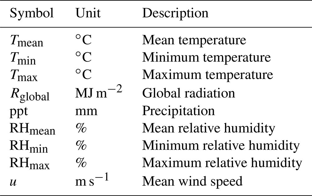
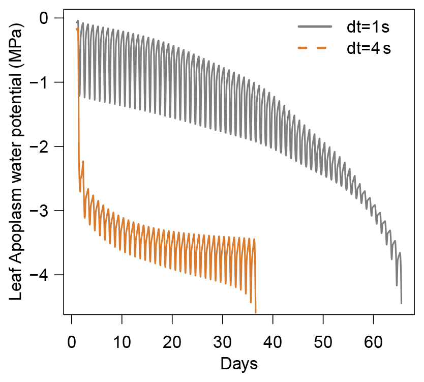
Figure B1Illustration of the constraint on δt due to the Courant–Friedrichs–Lewy (CFL) condition in SurEau-Ecos. Numerical instabilities are observed when .
Table B2The main physiological parameters of plant compartments used for the comparison between SurEau and SurEau-Ecos.
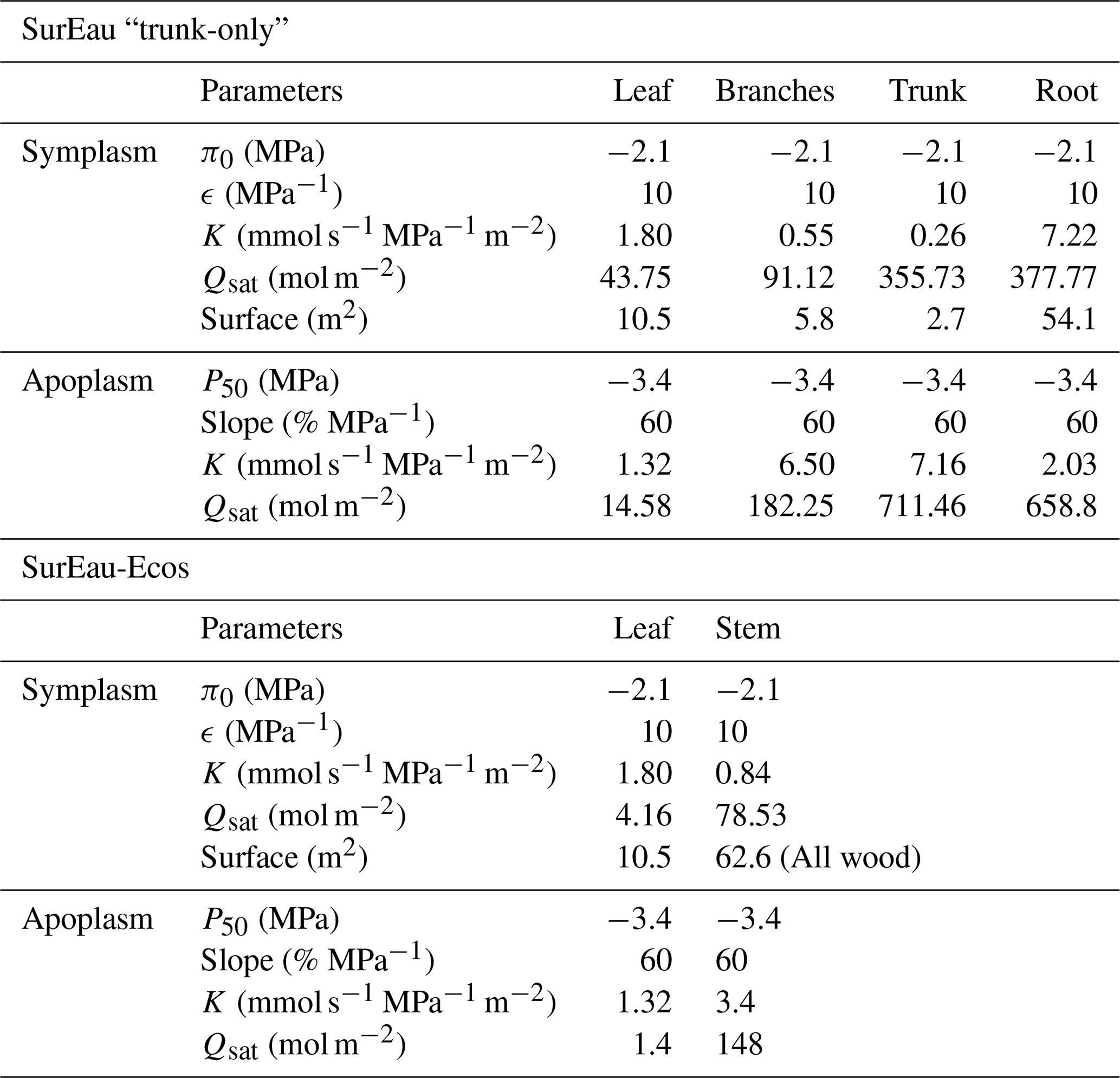
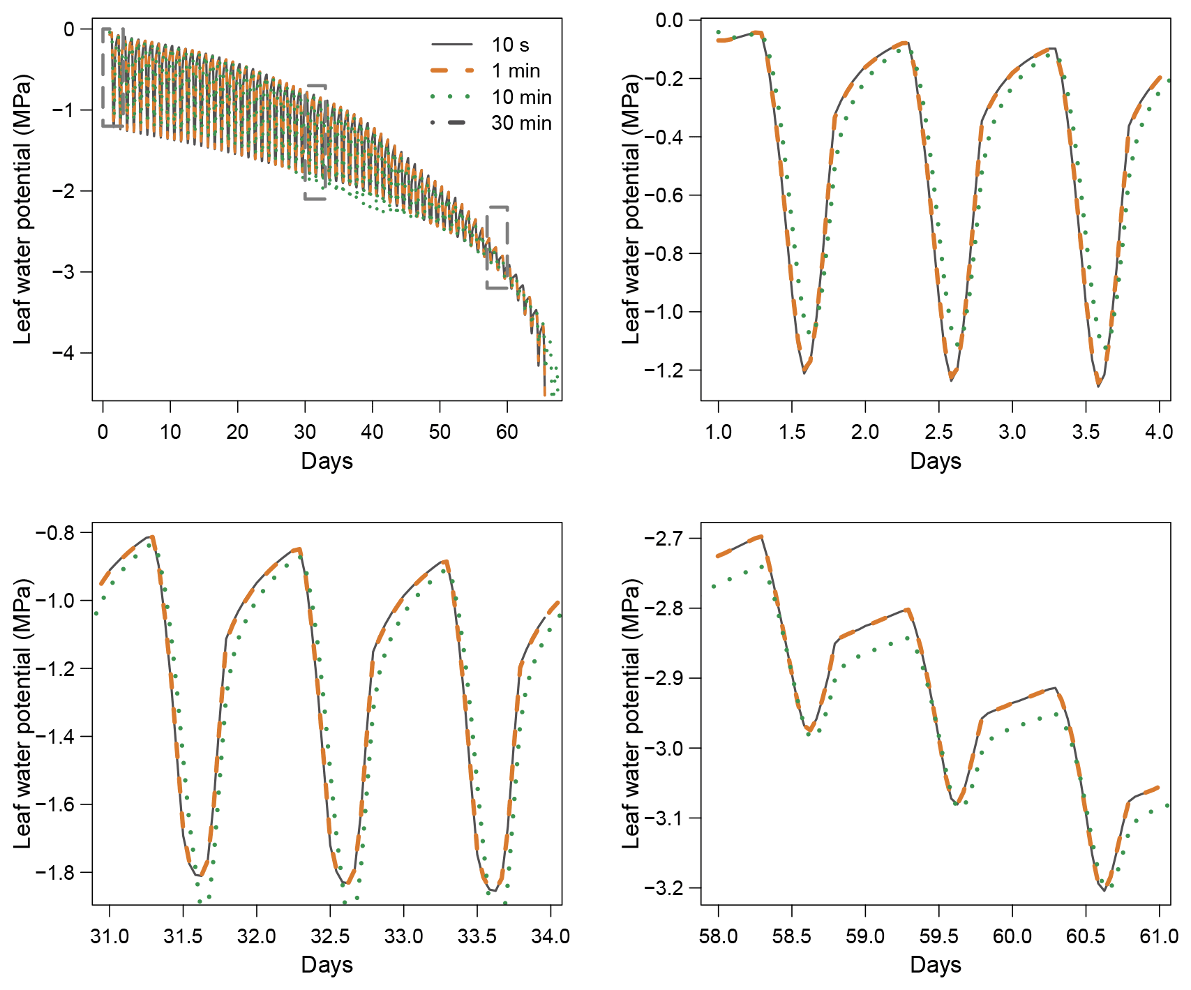
Figure B2Impact of the time step (δt) on simulation results with the implicit resolution scheme.
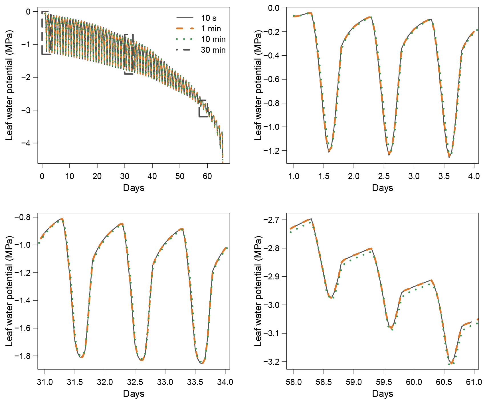
Figure B3Impact of the time step (δt) on simulation results with the semi-implicit resolution scheme.
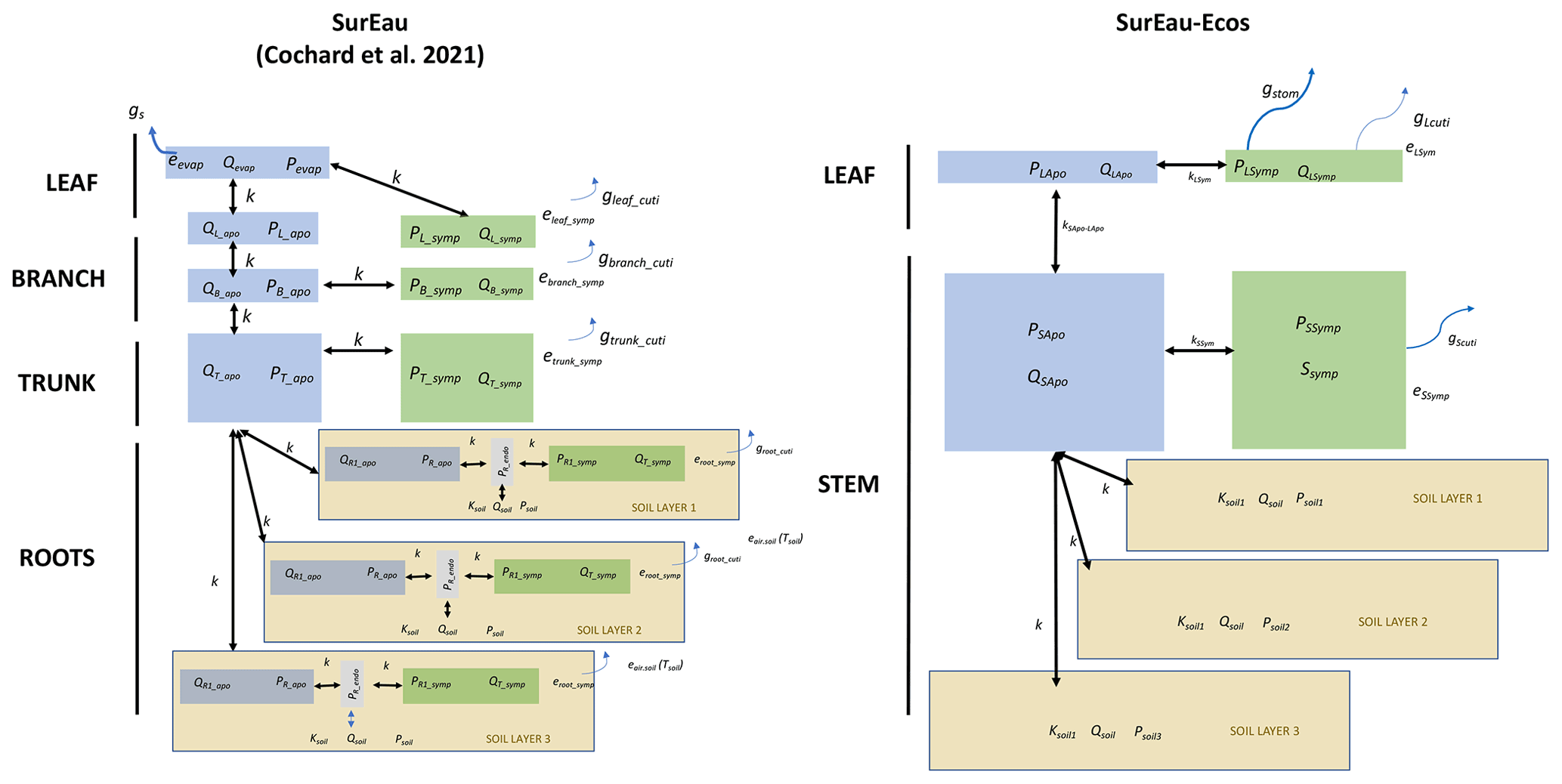
Figure B4Comparison between the plant architecture in SurEau and SurEau-Ecos. Q indicates the water quantities of the compartments, P the water potentials, k the hydraulic conductances, gs the gaseous stomatal conductances and gcuti the gaseous cuticular conductances. The subscripts “Apo”, “Sym” and “Endo” indicate the apoplasm, symplasm and endoderm compartments, respectively. The subscripts L, S, B, T and evap stand for leaf, stem, branch, trunk, root and evaporative sites, respectively.
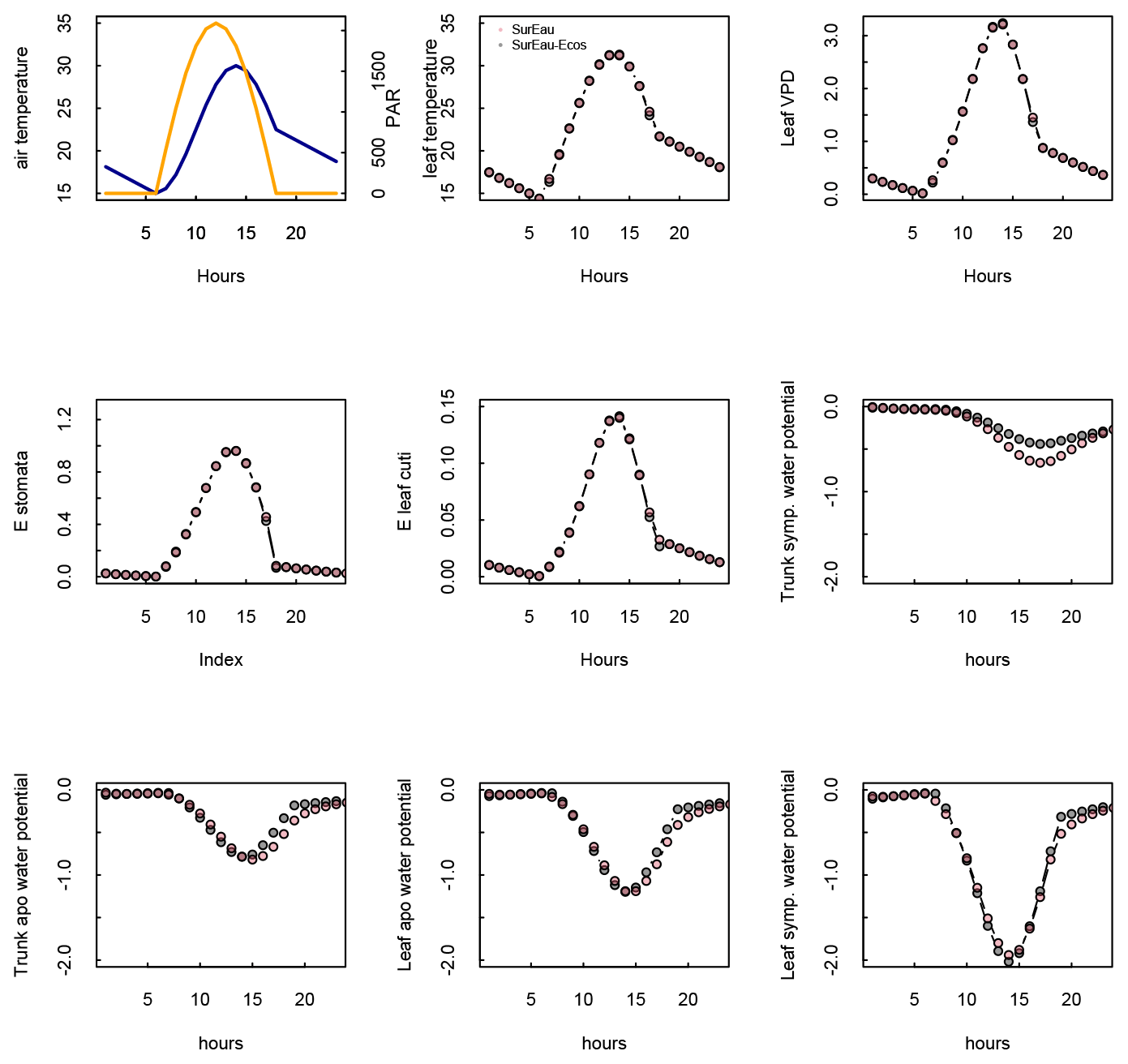
Figure B5Comparison of hourly outputs between SurEau and SurEau-Ecos for the first day of simulation. Climatic inputs (radiation, temperature and VPD) are shown in the upper panels.
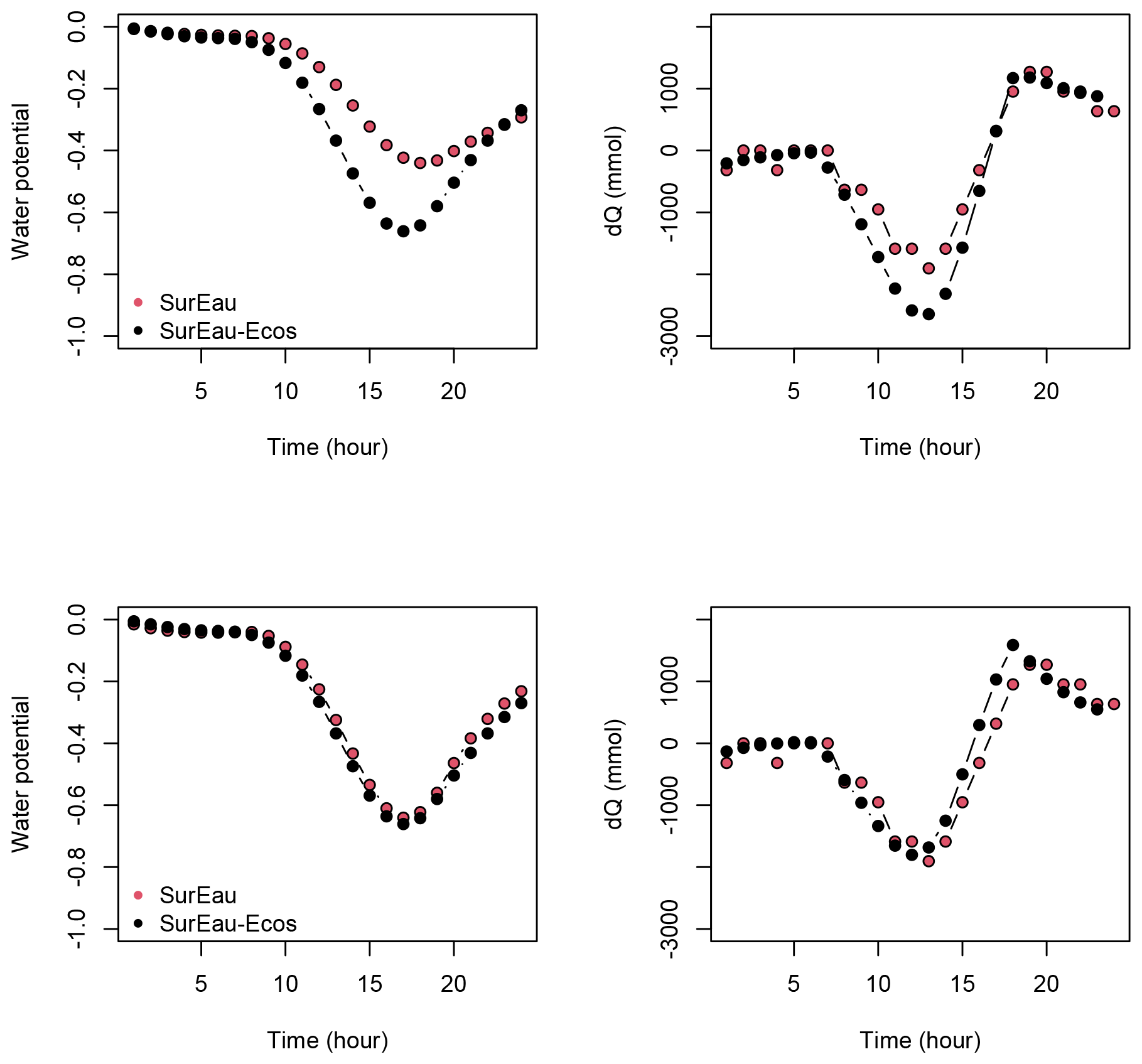
Figure B6Comparison of the water potential and the water discharge dynamics for the first day of simulation between the trunk compartment of SurEau and the stem compartment of SurEau-Ecos for two different parameterizations. In the upper row, SurEau-Ecos was parameterized with the stem symplasmic water volume computed as the sum of the symplasmic water volumes of the roots, trunk and branches of SurEau. In lower row, the stem symplasmic water volume of SurEau-Ecos was considered to be equivalent to the trunk water volume of SurEau (see Table B2 for details).
C1 Explicit scheme
Let
and let
Applying the explicit scheme (Eq. 48 in main text) to the four water balance equations (Eqs. 6 to 9 in main text) gives the following equations.
Equation (6) can be rearranged to determine :
Similarly, Eq. (7) gives :
Equations. (8) and (9) give and :
C2 Implicit scheme
By combining Eqs. (6), (7), (8) and (9) with the implicit discretization (Eq. 50), it is possible to analytically compute the unknown water potentials of each compartment at time n+1.
First, we eliminate in Eqs. (6) and (8) by summing and re-organizing the result as follows:
with
Next, let us define intermediate variables to ease the resolution with the following equations:
Now, Eq. (C5) can be rewritten as follows:
Similarly, eliminating in Eqs. (7) and (9) by summing and re-organizing the equation leads to the following result:
with
Similarly, by defining the following equations:
and
equation (C10) can be rewritten as follows:
Now, we eliminate from the simplified Eqs. (C9) and (C13) by summing and re-organizing it as follows:
Let
These equations can be combined to determine , and
We can now rearrange this to determine :
Knowing , we can determine from Eq. (C9):
In practice, because we do not know whether new cavitation events will occur during the time step, Eqs. (C6) and (C7) and (C11) and (C12) are first computed assuming that and did not change since the last time step. This will be correct for most time steps, except those when cavitation either starts or ends. At this stage, we should hence check whether solutions and are below or above and in order to eventually update or if needed. In cases where there is change (for time steps exactly corresponding to begin or end of cavitation events), the computation should be done again with actualized values of and .
Finally, knowing , we can solve from Eq. (8):
Knowing , we can solve from Eq. (9):
C3 Semi-implicit scheme
Let
and with
By combining Eqs. (6)–(9) with the semi-implicit Eq. (57), it leads to the following equations.
For ,
For ,
For ,
For ,
The model code and instructions on how to run the model version presented in this paper are available from https://doi.org/10.5281/zenodo.5878978 (Ruffault et al., 2022).
Weather simulation data of Global-Regional simulation model used in this study is available from the EURO-CORDEX initiative at https://www.euro-cordex.net/index.php.en (last access: 13 March 2021) for noncommercial research and educational purposes.
JR led the writing of the manuscript with input from all authors. JR and NMS coordinated the project. HC and JLD supervised the project. JR, NMS and FP developed the code and conducted the experiments. NMS developed a preliminary version of the code. FP designed the numerical resolutions of the model with inputs from NMS. All authors read and approved the manuscript.
The contact author has declared that none of the authors has any competing interests.
Publisher's note: Copernicus Publications remains neutral with regard to jurisdictional claims in published maps and institutional affiliations.
Julien Ruffault received funding from ECODIV department of INRAE. We acknowledge the INRAE ACCAF Metaprogram for its financial support of the project Drought&Fire. We thank Miquel De Cáceres and Xiangtao Xu for their careful reading of our original manuscript and their many insightful comments and suggestions.
This research has been supported by the Agence Nationale de la Recherche (grant no. ANR-18-CE20-0005). This study was completed with support from the Environmental Research and Development Program (SERDP) project through Forest Service Agreement 20-IJ-11221637-178.
This paper was edited by Hans Verbeeck and reviewed by Xiangtao Xu and one anonymous referee.
Abram, N. J., Henley, B. J., Sen Gupta, A., Lippmann, T. J. R., Clarke, H., Dowdy, A. J., Sharples, J. J., Nolan, R. H., Zhang, T., Wooster, M. J., Wurtzel, J. B., Meissner, K. J., Pitman, A. J., Ukkola, A. M., Murphy, B. P., Tapper, N. J., and Boer, M. M.: Connections of climate change and variability to large and extreme forest fires in southeast Australia, Commun. Earth Environ., 2, 1–17, https://doi.org/10.1038/s43247-020-00065-8, 2021.
Adams, H. D., Zeppel, M. J. B., Anderegg, W. R. L., Hartmann, H., Landhäusser, S. M., Tissue, D. T., Huxman, T. E., Hudson, P. J., Franz, T. E., Allen, C. D., Anderegg, L. D. L., Barron-Gafford, G. A., Beerling, D. J., Breshears, D. D., Brodribb, T. J., Bugmann, H., Cobb, R. C., Collins, A. D., Dickman, L. T., Duan, H., Ewers, B. E., Galiano, L., Galvez, D. A., Garcia-Forner, N., Gaylord, M. L., Germino, M. J., Gessler, A., Hacke, U. G., Hakamada, R., Hector, A., Jenkins, M. W., Kane, J. M., Kolb, T. E., Law, D. J., Lewis, J. D., Limousin, J.-M., Love, D. M., Macalady, A. K., Martínez-Vilalta, J., Mencuccini, M., Mitchell, P. J., Muss, J. D., O'Brien, M. J., O'Grady, A. P., Pangle, R. E., Pinkard, E. A., Piper, F. I., Plaut, J. A., Pockman, W. T., Quirk, J., Reinhardt, K., Ripullone, F., Ryan, M. G., Sala, A., Sevanto, S., Sperry, J. S., Vargas, R., Vennetier, M., Way, D. A., Xu, C., Yepez, E. A., and McDowell, N. G.: A multi-species synthesis of physiological mechanisms in drought-induced tree mortality, Nat. Ecol. Evol., 1, 1285–1291, https://doi.org/10.1038/s41559-017-0248-x, 2017.
Allen, C. D., Breshears, D. D., and McDowell, N. G.: On underestimation of global vulnerability to tree mortality and forest die-off from hotter drought in the Anthropocene, Ecosphere, 6, art129, https://doi.org/10.1890/ES15-00203.1, 2015.
Arend, M., Link, R. M., Zahnd, C., Hoch, G., Schuldt, B., and Kahmen, A.: Lack of hydraulic recovery as a cause of post-drought foliage reduction and canopy decline in European beech, New Phytol., 234, 1195–1205, https://doi.org/10.1111/nph.18065, 2022.
Bartlett, M. K., Scoffoni, C., and Sack, L.: The determinants of leaf turgor loss point and prediction of drought tolerance of species and biomes: A global meta-analysis, Ecol. Lett., 15, 393–405, https://doi.org/10.1111/j.1461-0248.2012.01751.x, 2012.
Bartlett, M. K., Klein, T., Jansen, S., Choat, B., and Sack, L.: The correlations and sequence of plant stomatal, hydraulic, and wilting responses to drought, P. Natl. Acad. Sci. USA, 113, 13098–13103, https://doi.org/10.1073/pnas.1604088113, 2016.
Billon, L. M., Blackman, C. J., Cochard, H., Badel, E., Hitmi, A., Cartailler, J., Souchal, R., and Torres-Ruiz, J. M.: The DroughtBox: A new tool for phenotyping residual branch conductance and its temperature dependence during drought, Plant Cell Environ., 43, 1584–1594, https://doi.org/10.1111/pce.13750, 2020.
Brodribb, T. J., Powers, J., Cochard, H., and Choat, B.: Hanging by a thread? Forests and drought, Science, 368, 261–266, https://doi.org/10.1126/science.aat7631, 2020.
Cheaib, A., Badeau, V., Boe, J., Chuine, I., Delire, C., Dufrêne, E., François, C., Gritti, E. S., Legay, M., Pagé, C., Thuiller, W., Viovy, N., and Leadley, P.: Climate change impacts on tree ranges: Model intercomparison facilitates understanding and quantification of uncertainty, Ecol. Lett., 15, 533–544, https://doi.org/10.1111/j.1461-0248.2012.01764.x, 2012.
Choat, B., Jansen, S., Brodribb, T. J., Cochard, H., Delzon, S., Bhaskar, R., Bucci, S. J., Feild, T. S., Gleason, S. M., Hacke, U. G., Jacobsen, A. L., Lens, F., Maherali, H., Martínez-Vilalta, J., Mayr, S., Mencuccini, M., Mitchell, P. J., Nardini, A., Pittermann, J., Pratt, R. B., Sperry, J. S., Westoby, M., Wright, I. J., and Zanne, A. E.: Global convergence in the vulnerability of forests to drought, Nature, 491, 4–8, https://doi.org/10.1038/nature11688, 2012.
Choat, B., Brodribb, T. J., Brodersen, C. R., Duursma, R. A., López, R., and Medlyn, B. E.: Triggers of tree mortality under drought, Nature, 558, 531–539, https://doi.org/10.1038/s41586-018-0240-x, 2018.
Christoffersen, B. O., Gloor, M., Fauset, S., Fyllas, N. M., Galbraith, D. R., Baker, T. R., Kruijt, B., Rowland, L., Fisher, R. A., Binks, O. J., Sevanto, S., Xu, C., Jansen, S., Choat, B., Mencuccini, M., McDowell, N. G., and Meir, P.: Linking hydraulic traits to tropical forest function in a size-structured and trait-driven model (TFS v.1-Hydro), Geosci. Model Dev., 9, 4227–4255, https://doi.org/10.5194/gmd-9-4227-2016, 2016.
Chuine, I. and Cour, P.: Climatic determinants of budburst seasonality in four temperate-zone tree species, New Phytol., 143, 339–349, 1999.
Cochard, H.: A new mechanism for tree mortality due to drought and heatwaves, Peer Community J., 1, e36, https://doi.org/10.24072/PCJOURNAL.45, 2021.
Cochard, H., Pimont, F., Ruffault, J., and Martin-StPaul, N.: SurEau: a mechanistic model of plant water relations under extreme drought, Ann. For. Sci., 78, 1–23, https://doi.org/10.1007/s13595-021-01067-y, 2021.
Couvreur, V., Ledder, G., Manzoni, S., Way, D. A., Muller, E. B., and Russo, S. E.: Water transport through tall trees: A vertically explicit, analytical model of xylem hydraulic conductance in stems, Plant Cell Environ., 41, 1821–1839, https://doi.org/10.1111/pce.13322, 2018.
Cruiziat, P., Cochard, H., and Améglio, T.: Hydraulic architecture of trees: main concepts and results, Ann. For. Sci., 59, 723–752, https://doi.org/10.1051/forest:2002060, 2002.
De Cáceres, M., Martínez-Vilalta, J., Coll, L., Llorens, P., Casals, P., Poyatos, R., Pausas, J. G., and Brotons, L.: Coupling a water balance model with forest inventory data to predict drought stress: The role of forest structural changes vs. climate changes, Agric. For. Meteorol., 213, 77–90, https://doi.org/10.1016/j.agrformet.2015.06.012, 2015.
De Cáceres, M., Mencuccini, M., Martin-StPaul, N., Limousin, J. M., Coll, L., Poyatos, R., Cabon, A., Granda, V., Forner, A., Valladares, F., and Martínez-Vilalta, J.: Unravelling the effect of species mixing on water use and drought stress in Mediterranean forests: A modelling approach, Agric. For. Meteorol., 296, 108233, https://doi.org/10.1016/j.agrformet.2020.108233, 2021.
De Kauwe, M. G., Medlyn, B. E., Ukkola, A. M., Mu, M., Sabot, M. E. B., Pitman, A. J., Meir, P., Cernusak, L. A., Rifai, S. W., Choat, B., Tissue, D. T., Blackman, C. J., Li, X., Roderick, M., and Briggs, P. R.: Identifying areas at risk of drought-induced tree mortality across South-Eastern Australia, Glob. Change Biol., 26, 5716–5733, https://doi.org/10.1111/gcb.15215, 2020.
Domec, J. C., Smith, D. D., and McCulloh, K. A.: A synthesis of the effects of atmospheric carbon dioxide enrichment on plant hydraulics: implications for whole-plant water use efficiency and resistance to drought, Plant Cell Environ., 40, 921–937, https://doi.org/10.1111/pce.12843, 2017.
Dufour-Kowalski, S., Courbaud, B., Dreyfus, P., Meredieu, C., and De Coligny, F.: Capsis: An open software framework and community for forest growth modelling, Ann. Forest Sci., 221–233, https://doi.org/10.1007/s13595-011-0140-9, 2012.
Dufrêne, E., Davi, H., François, C., Maire, G. le, Dantec, V. L., and Granier, A.: Modelling carbon and water cycles in a beech forest: Part I: Model description and uncertainty analysis on modelled NEE, Ecol. Model., 185, 407–436, https://doi.org/10.1016/j.ecolmodel.2005.01.004, 2005.
Dutykh, D.: How to overcome the Courant-Friedrichs-Lewy condition of explicit discretizations?, Numer. Methods Diffus. Phenom. Build. Phys., 103–120, https://doi.org/10.1007/978-3-030-31574-0_5, 2016.
Duursma, R. A., Blackman, C. J., Lopéz, R., Martin-StPaul, N. K., Cochard, H., and Medlyn, B. E.: On the minimum leaf conductance: its role in models of plant water use, and ecological and environmental controls, New Phytol., 221, 693–705, https://doi.org/10.1111/nph.15395, 2019.
Fargeon, H., Pimont, F., Martin-StPaul, N., De Caceres, M., Ruffault, J., Barbero, R., and Dupuy, J. L.: Projections of fire danger under climate change over France: where do the greatest uncertainties lie?, Clim. Change, 160, 479–493, https://doi.org/10.1007/s10584-019-02629-w, 2020.
Fatichi, S., Pappas, C., and Ivanov, V. Y.: Modeling plant–water interactions: an ecohydrological overview from the cell to the global scale, Wiley Interdiscip. Rev. Water, 3, 327–368, https://doi.org/10.1002/wat2.1125, 2016.
Feng, X., Ackerly, D. D., Dawson, T. E., Manzoni, S., Skelton, R. P., Vico, G., and Thompson, S. E.: The ecohydrological context of drought and classification of plant responses, Ecol. Lett., 21, 1723–1736, https://doi.org/10.1111/ele.13139, 2018.
Fettig, C. J., Mortenson, L. A., Bulaon, B. M., and Foulk, P. B.: Tree mortality following drought in the central and southern Sierra Nevada, California, U.S., For. Ecol. Manag., 432, 164–178, https://doi.org/10.1016/j.foreco.2018.09.006, 2019.
Granier, A., Bréda, N., Biron, P., and Villette, S.: A lumped water balance model to evaluate duration and intensity of drought constraints in forest stands, Ecol. Model., 116, 269–283, https://doi.org/10.1016/S0304-3800(98)00205-1, 1999.
Guillemot, J., Martin-StPaul, N. K., Bulascoschi, L., Poorter, L., Morin, X., Pinho, B. X., le Maire, G., R. L. Bittencourt, P., Oliveira, R. S., Bongers, F., Brouwer, R., Pereira, L., Gonzalez Melo, G. A., Boonman, C. C. F., Brown, K. A., Cerabolini, B. E. L., Niinemets, Ü., Onoda, Y., Schneider, J. V., Sheremetiev, S., and Brancalion, P. H. S.: Small and slow is safe: On the drought tolerance of tropical tree species, Glob. Change Biol., 28, 2622–2638, https://doi.org/10.1111/gcb.16082, 2022.
Gupta, S., Hengl, T., Lehmann, P., Bonetti, S., and Or, D.: SoilKsatDB: global database of soil saturated hydraulic conductivity measurements for geoscience applications, Earth Syst. Sci. Data, 13, 1593–1612, https://doi.org/10.5194/essd-13-1593-2021, 2021.
Hengl, T., Jesus, J. M. de, Heuvelink, G. B. M., Gonzalez, M. R., Kilibarda, M., Blagotiæ, A., Shangguan, W., Wright, M. N., Geng, X., Bauer-Marschallinger, B., Guevara, M. A., Vargas, R., MacMillan, R. A., Batjes, N. H., Leenaars, J. G. B., Ribeiro, E., Wheeler, I., Mantel, S., and Kempen, B.: SoilGrids250m: Global gridded soil information based on machine learning, PLOS ONE, 12, e0169748, https://doi.org/10.1371/journal.pone.0169748, 2017.
Hoff, C. and Rambal, S.: An examination of the interaction between climate, soil and leaf area index in a Quercus ilex ecosystem, Ann. For. Sci., 60, 153–161, https://doi.org/10.1051/forest:2003008, 2003.
Hölttä, T., Cochard, H., Nikinmaa, E., and Mencuccini, M.: Capacitive effect of cavitation in xylem conduits: results from a dynamic model, Plant Cell Environ., 32, 10–21, 2009.
Jackson, R. B., Canadell, J., Ehleringer, J. R., Mooney, H. A., Sala, O. E., and Schulze, E. D.: A global analysis of root distributions for terrestrial biomes, Oecologia, 108, 389–411, https://doi.org/10.1007/BF00333714, 1996.
Jactel, H., Petit, J., Desprez-Loustau, M. L., Delzon, S., Piou, D., Battisti, A., and Koricheva, J.: Drought effects on damage by forest insects and pathogens: A meta-analysis, Glob. Change Biol., 18, 267–276, https://doi.org/10.1111/j.1365-2486.2011.02512.x, 2012.
Jarvis, P. G.: The interpretation of the variations in leaf water potential and stomatal conductance found in canopies in the field, Philos. T. Roy. Soc. Lond. B, 273, 593–610, https://doi.org/10.1098/rstb.1976.0035, 1976.
Jones, H. G.: Plants and microclimate: A quantitative approach to environmental plant physiology, Cambridge University Press, https://doi.org/10.1017/CBO9780511845727, 2013.
Kattge, J., Díaz, S., Lavorel, S., Prentice, I. C., Leadley, P., Bönisch, G., Garnier, E., Westoby, M., Reich, P. B., Wright, I. J., Cornelissen, J. H. C., Violle, C., Harrison, S. P., Van BODEGOM, P. M., Reichstein, M., Enquist, B. J., Soudzilovskaia, N. A., Ackerly, D. D., Anand, M., Atkin, O., Bahn, M., Baker, T. R., Baldocchi, D., Bekker, R., Blanco, C. C., Blonder, B., Bond, W. J., Bradstock, R., Bunker, D. E., Casanoves, F., Cavender-Bares, J., Chambers, J. Q., Chapin Iii, F. S., Chave, J., Coomes, D., Cornwell, W. K., Craine, J. M., Dobrin, B. H., Duarte, L., Durka, W., Elser, J., Esser, G., Estiarte, M., Fagan, W. F., Fang, J., Fernández-Méndez, F., Fidelis, A., Finegan, B., Flores, O., Ford, H., Frank, D., Freschet, G. T., Fyllas, N. M., Gallagher, R. V., Green, W. A., Gutierrez, A. G., Hickler, T., Higgins, S. I., Hodgson, J. G., Jalili, A., Jansen, S., Joly, C. A., Kerkhoff, A. J., Kirkup, D., Kitajima, K., Kleyer, M., Klotz, S., Knops, J. M. H., Kramer, K., Kühn, I., Kurokawa, H., Laughlin, D., Lee, T. D., Leishman, M., Lens, F., Lenz, T., Lewis, S. L., Lloyd, J., Llusià, J., Louault, F., Ma, S., Mahecha, M. D., Manning, P., Massad, T., Medlyn, B. E., Messier, J., Moles, A. T., Müller, S. C., Nadrowski, K., Naeem, S., Niinemets, Ü., Nöllert, S., Nüske, A., Ogaya, R., Oleksyn, J., Onipchenko, V. G., Onoda, Y., Ordoñez, J., Overbeck, G., Ozinga, W. A., Patiño, S., Paula, S., Pausas, J. G., Peñuelas, J., Phillips, O. L., Pillar, V., Poorter, H., Poorter, L., Poschlod, P., Prinzing, A., Proulx, R., Rammig, A., Reinsch, S., Reu, B., Sack, L., Salgado-Negret, B., Sardans, J., Shiodera, S., Shipley, B., Siefert, A., Sosinski, E., Soussana, J.-F., Swaine, E., Swenson, N., Thompson, K., Thornton, P., Waldram, M., Weiher, E., White, M., White, S., Wright, S. J., Yguel, B., Zaehle, S., Zanne, A. E., and Wirth, C.: TRY – a global database of plant traits, Glob. Change Biol., 17, 2905–2935, https://doi.org/10.1111/j.1365-2486.2011.02451.x, 2011.
Kennedy, D., Swenson, S., Oleson, K. W., Lawrence, D. M., Fisher, R., Lola da Costa, A. C., and Gentine, P.: Implementing Plant Hydraulics in the Community Land Model, Version 5, J. Adv. Model. Earth Syst., 11, 485–513, https://doi.org/10.1029/2018MS001500, 2019.
Klein, T.: The variability of stomatal sensitivity to leaf water potential across tree species indicates a continuum between isohydric and anisohydric behaviours, Funct. Ecol., 28, 1313–1320, https://doi.org/10.1111/1365-2435.12289, 2014.
Kotlarski, S., Keuler, K., Christensen, O. B., Colette, A., Déqué, M., Gobiet, A., Goergen, K., Jacob, D., Lüthi, D., van Meijgaard, E., Nikulin, G., Schär, C., Teichmann, C., Vautard, R., Warrach-Sagi, K., and Wulfmeyer, V.: Regional climate modeling on European scales: a joint standard evaluation of the EURO-CORDEX RCM ensemble, Geosci. Model Dev., 7, 1297–1333, https://doi.org/10.5194/gmd-7-1297-2014, 2014.
Lemaire, C., Blackman, C. J., Cochard, H., Menezes-Silva, P. E., Torres-Ruiz, J. M., and Herbette, S.: Acclimation of hydraulic and morphological traits to water deficit delays hydraulic failure during simulated drought in poplar, Tree Physiol., 41, 2008–2021, 2021.
Lens, F., Picon-Cochard, C., Delmas, C. E. L., Signarbieux, C., Buttler, A., Cochard, H., Jansen, S., Chauvin, T., Doria, L. C., Del Arco, M., and Delzon, S.: Herbaceous angiosperms are not more vulnerable to drought-induced embolism than angiosperm trees, Plant Physiol., 172, 661–667, https://doi.org/10.1104/PP.16.00829, 2016.
Li, L., Yang, Z., Matheny, A. M., Zheng, H., Swenson, S. C., Lawrence, D. M., Barlage, M., Yan, B., McDowell, N. G., and Leung, L. R.: Representation of Plant Hydraulics in the Noah-MP Land Surface Model: Model Development and Multi-scale Evaluation, J. Adv. Model. Earth Syst., 13, e2020MS002214, https://doi.org/10.1029/2020ms002214, 2021.
Lin, Y.-S., Medlyn, B. E., Duursma, R. A., Prentice, I. C., Wang, H., Baig, S., Eamus, D., de Dios, V. R., Mitchell, P., Ellsworth, D. S., de Beeck, M. O., Wallin, G., Uddling, J., Tarvainen, L., Linderson, M.-L., Cernusak, L. A., Nippert, J. B., Ocheltree, T. W., Tissue, D. T., Martin-StPaul, N. K., Rogers, A., Warren, J. M., De Angelis, P., Hikosaka, K., Han, Q., Onoda, Y., Gimeno, T. E., Barton, C. V. M., Bennie, J., Bonal, D., Bosc, A., Löw, M., Macinins-Ng, C., Rey, A., Rowland, L., Setterfield, S. A., Tausz-Posch, S., Zaragoza-Castells, J., Broadmeadow, M. S. J., Drake, J. E., Freeman, M., Ghannoum, O., Hutley, L. B., Kelly, J. W., Kikuzawa, K., Kolari, P., Koyama, K., Limousin, J.-M., Meir, P., Lola da Costa, A. C., Mikkelsen, T. N., Salinas, N., Sun, W., and Wingate, L.: Optimal stomatal behaviour around the world, Nat. Clim. Change, 5, 459–464, https://doi.org/10.1038/nclimate2550, 2015.
López, R., Cano, F. J., Martin-StPaul, N. K., Cochard, H., and Choat, B.: Coordination of stem and leaf traits define different strategies to regulate water loss and tolerance ranges to aridity, New Phytol., 230, 497–509, 2021.
Mackay, D. S., Ahl, D. E., Ewers, B. E., Samanta, S., Gower, S. T., and Burrows, S. N.: Physiological tradeoffs in the parameterization of a model of canopy transpiration, Adv. Water Resour., 26, 179–194, https://doi.org/10.1016/S0309-1708(02)00090-8, 2003.
Mantova, M., Menezes-Silva, P. E., Badel, E., Cochard, H., and Torres-Ruiz, J. M.: The interplay of hydraulic failure and cell vitality explains tree capacity to recover from drought, Physiol. Plant., 172, 13331, https://doi.org/10.1111/ppl.13331, 2021.
Martinez-Vilalta, J., Anderegg, W. R. L., Sapes, G., and Sala, A.: Greater focus on water pools may improve our ability to understand and anticipate drought-induced mortality in plants, New Phytol., 223, 22–32, https://doi.org/10.1111/nph.15644, 2019.
Martin-StPaul, N., Delzon, S., and Cochard, H.: Plant resistance to drought depends on timely stomatal closure, Ecol. Lett., 20, 1437–1447, https://doi.org/10.1111/ele.12851, 2017.
McDowell, N. G., Brodribb, T. J., and Nardini, A.: Hydraulics in the 21st century, New Phytol., 224, 537–542, https://doi.org/10.1111/nph.16151, 2019.
McDowell, N. G., Sapes, G., Pivovaroff, A., Adams, H. D., Allen, C. D., Anderegg, W. R. L., Arend, M., Breshears, D. D., Brodribb, T., Choat, B., Cochard, H., De Cáceres, M., De Kauwe, M. G., Grossiord, C., Hammond, W. M., Hartmann, H., Hoch, G., Kahmen, A., Klein, T., Mackay, D. S., Mantova, M., Martínez-Vilalta, J., Medlyn, B. E., Mencuccini, M., Nardini, A., Oliveira, R. S., Sala, A., Tissue, D. T., Torres-Ruiz, J. M., Trowbridge, A. M., Trugman, A. T., Wiley, E., and Xu, C.: Mechanisms of woody-plant mortality under rising drought, CO2 and vapour pressure deficit, Nat. Rev. Earth Environ., 3, 294–308, https://doi.org/10.1038/s43017-022-00272-1, 2022.
Meinzer, F. C., Woodruff, D. R., Domec, J.-C., Goldstein, G., Campanello, P. I., Gatti, M. G., and Villalobos-Vega, R.: Coordination of leaf and stem water transport properties in tropical forest trees, Oecologia, 156, 31–41, https://doi.org/10.1007/s00442-008-0974-5, 2008.
Meir, P., Meir, P., Mencuccini, M., and Dewar, R. C.: Tansley insight Drought-related tree mortality: addressing the gaps in understanding and prediction, New Phytol., 207, 28–33, 2015.
Mencuccini, M., Manzoni, S., and Christoffersen, B.: Modelling water fluxes in plants: from tissues to biosphere, New Phytol., 222, 1207–1222, https://doi.org/10.1111/nph.15681, 2019.
Moreaux, V., Martel, S., Bosc, A., Picart, D., Achat, D., Moisy, C., Aussenac, R., Chipeaux, C., Bonnefond, J.-M., Figuères, S., Trichet, P., Vezy, R., Badeau, V., Longdoz, B., Granier, A., Roupsard, O., Nicolas, M., Pilegaard, K., Matteucci, G., Jolivet, C., Black, A. T., Picard, O., and Loustau, D.: Energy, water and carbon exchanges in managed forest ecosystems: description, sensitivity analysis and evaluation of the INRAE GO+ model, version 3.0, Geosci. Model Dev., 13, 5973–6009, https://doi.org/10.5194/gmd-13-5973-2020, 2020.
Morin, X., Bugmann, H., de Coligny, F., Martin-StPaul, N., Cailleret, M., Limousin, J.-M., Ourcival, J.-M., Prevosto, B., Simioni, G., Toigo, M., Vennetier, M., Catteau, E., and Guillemot, J.: Beyond forest succession: A gap model to study ecosystem functioning and tree community composition under climate change, Funct. Ecol., 35, 955–975, https://doi.org/10.1111/1365-2435.13760, 2021.
Mouillot, F., Rambal, S., and Lavorel, S.: A generic process-based SImulator for meditERRanean landscApes (SIERRA): design and validation exercises, For. Ecol. Manag., 147, 75–97, 2001.
Nolan, R. H., Blackman, C. J., de Dios, V. R., Choat, B., Medlyn, B. E., Li, X., Bradstock, R. A., and Boer, M. M.: Linking Forest Flammability and Plant Vulnerability to Drought, Forests, 11, 779, https://doi.org/10.3390/f11070779, 2020.
Pammenter, N. W. and Vander Willigen, C.: A mathematical and statistical analysis of the curves illustrating vulnerability of xylem to cavitation, Tree Physiol., 18, 589–593, 1998.
Pimont, F., Ruffault, J., Martin-StPaul, N. K., and Dupuy, J.-L.: Why is the effect of live fuel moisture content on fire rate of spread underestimated in field experiments in shrublands?, Int. J. Wildland Fire, 28, 127–137, https://doi.org/10.1071/WF18091, 2019.
Rambal, S.: The differential role of mechanisms for drought resistance in a Mediterranean evergreen shrub: a simulation approach, Plant Cell Environ., 16, 35–44, https://doi.org/10.1111/j.1365-3040.1993.tb00842.x, 1993.
R Core Team: R: A Language and Environment for Statistical Computing, R Foundation for Statistical Computing, Vienna, Austria, 2020.
Riederer, M. and Schreiber, L.: Protecting against water loss: analysis of the barrier properties of plant cuticles, J. Exp. Bot., 52, 2023–2032, https://doi.org/10.1093/jexbot/52.363.2023, 2001.
Rowland, L., Martínez-Vilalta, J., and Mencuccini, M.: Hard times for high expectations from hydraulics: predicting drought-induced forest mortality at landscape scales remains a challenge, New Phytol., 230, 1685–1687, https://doi.org/10.1111/nph.17317, 2021.
Ruffault, J., Martin-StPaul, N. K. N., Rambal, S., and Mouillot, F.: Differential regional responses in drought length, intensity and timing to recent climate changes in a Mediterranean forested ecosystem, Clim. Change, 117, 103–117, https://doi.org/10.1007/s10584-012-0559-5, 2013.
Ruffault, J., Martin-StPaul, N. K., Duffet, C., Goge, F., and Mouillot, F.: Projecting future drought in Mediterranean forests: Bias correction of climate models matters!, Theor. Appl. Climatol., 117, 113–122, https://doi.org/10.1007/s00704-013-0992-z, 2014.
Ruffault, J., Curt, T., Martin-StPaul, N. K., Moron, V., and Trigo, R. M.: Extreme wildfire events are linked to global-change-type droughts in the northern Mediterranean, Nat. Hazards Earth Syst. Sci., 18, 847–856, https://doi.org/10.5194/nhess-18-847-2018, 2018a.
Ruffault, J., Martin-StPaul, N., Pimont, F., and Dupuy, J.-L.: How well do meteorological drought indices predict live fuel moisture content (LFMC)? An assessment for wildfire research and operations in Mediterranean ecosystems, Agric. For. Meteorol., 262, 391–401, https://doi.org/10.1016/j.agrformet.2018.07.031, 2018b.
Ruffault, J., Curt, T., Moron, V., Trigo, R. M., Mouillot, F., Koutsias, N., Pimont, F., Martin-StPaul, N. K., Barbero, R., Dupuy, J. L., Russo, A., and Belhadj-Kheder, C.: Increased likelihood of heat-induced large wildfires in the Mediterranean Basin, Sci. Rep.-UK, 10, 13790, https://doi.org/10.1101/2020.01.09.896878, 2020.
Ruffault, J., Martin-StPaul, N., and Pimont, F.: SurEau-Ecos v2.0.1 (v2.0.1), Zenodo [code], https://doi.org/10.5281/zenodo.5878978, 2022.
Schuldt, B., Buras, A., Arend, M., Vitasse, Y., Beierkuhnlein, C., Damm, A., Gharun, M., Grams, T. E. E., Hauck, M., Hajek, P., Hartmann, H., Hiltbrunner, E., Hoch, G., Holloway-Phillips, M., Körner, C., Larysch, E., Lübbe, T., Nelson, D. B., Rammig, A., Rigling, A., Rose, L., Ruehr, N. K., Schumann, K., Weiser, F., Werner, C., Wohlgemuth, T., Zang, C. S., and Kahmen, A.: A first assessment of the impact of the extreme 2018 summer drought on Central European forests, Basic Appl. Ecol., 45, 86–103, https://doi.org/10.1016/j.baae.2020.04.003, 2020.
Seidl, R., Schelhaas, M.-J., Rammer, W., and Verkerk, P. J.: Increasing forest disturbances in Europe and their impact on carbon storage, Nat. Clim. Change, 4, 806–810, 2014.
Sergent, A. S., Varela, S. A., Barigah, T. S., Badel, E., Cochard, H., Dalla-Salda, G., Delzon, S., Fernández, M. E., Guillemot, J., Gyenge, J., Lamarque, L. J., Martinez-Meier, A., Rozenberg, P., Torres-Ruiz, J. M., and Martin-StPaul, N. K.: A comparison of five methods to assess embolism resistance in trees, For. Ecol. Manag., 468, 118175, https://doi.org/10.1016/j.foreco.2020.118175, 2020.
Sitch, S., Smith, B., Prentice, I. C., Arneth, A., Bondeau, A., Cramer, W., Kaplan, J. O., Levis, S., Lucht, W., and Sykes, M. T.: Evaluation of ecosystem dynamics, plant geography and terrestrial carbon cycling in the LPJ dynamic global vegetation model, Glob. Change Biol., 9, 161–185, 2003.
Sobol, I. M.: Global sensitivity indices for nonlinear mathematical models and their Monte Carlo estimates, Math. Comput. Simul., 55, 271–280, 2001.
Sperry, J. S., Adler, F. R., Campbell, G. S., and Comstock, J. P.: Limitation of plant water use by rhizosphere and xylem conductance: results from a model, Plant Cell Environ., 21, 347–359, https://doi.org/10.1046/j.1365-3040.1998.00287.x, 1998.
Sperry, J. S., Venturas, M. D., Anderegg, W. R. L., Mencuccini, M., Mackay, D. S., Wang, Y., and Love, D. M.: Predicting stomatal responses to the environment from the optimization of photosynthetic gain and hydraulic cost, Plant Cell Environ., 40, 816–830, 2017.
Sterck, F., Markesteijn, L., Schieving, F., and Poorter, L.: Functional traits determine trade-offs and niches in a tropical forest community, P. Natl. Acad. Sci. USA, 108, 20627–20632, https://doi.org/10.1073/pnas.1106950108, 2011.
Tóth, B., Weynants, M., Pásztor, L., and Hengl, T.: 3D soil hydraulic database of Europe at 250 m resolution, Hydrol. Process., 31, 2662–2666, https://doi.org/10.1002/hyp.11203, 2017.
Trenberth, K. E., Dai, A., Van Der Schrier, G., Jones, P. D., Barichivich, J., Briffa, K. R., and Sheffield, J.: Global warming and changes in drought, Nat. Clim. Change, 4, 17–22, 2014.
Trugman, A. T., Anderegg, L. D. L., Anderegg, W. R. L., Das, A. J., and Stephenson, N. L.: Why is Tree Drought Mortality so Hard to Predict?, Trends Ecol. Evol., 36, 520–532, https://doi.org/10.1016/j.tree.2021.02.001, 2021.
Tuzet, A., Granier, A., Betsch, P., Peiffer, M., and Perrier, A.: Modelling hydraulic functioning of an adult beech stand under non-limiting soil water and severe drought condition, Ecol. Model., 348, 56–77, https://doi.org/10.1016/j.ecolmodel.2017.01.007, 2017.
Tyree, M. T. and Ewers, F. W.: The hydraulic architecture of trees and other woody plants, New Phytol., 119, 345–360, https://doi.org/10.1111/j.1469-8137.1991.tb00035.x, 1991.
Tyree, M. T. and Hammel, H. T.: The Measurement of the turgor pressure and the water relations of plants by the pressure-bomb technique, J. Exp. Bot., 23, 267–282, https://doi.org/10.1093/jxb/23.1.267, 1972.
Tyree, M. T. and Yang, S.: Water-storage capacity ofThuja, Tsuga andAcer stems measured by dehydration isotherms, Planta, 182, 420–426, 1990.
van Genuchten, M. T.: A closed-form equation for predicting the hydraulic conductivity of unsaturated soils, Soil Sci. Soc. Am. J., 44, 892, https://doi.org/10.2136/sssaj1980.03615995004400050002x, 1980.
Venturas, M. D., Todd, H. N., Trugman, A. T., and Anderegg, W. R. L.: Understanding and predicting forest mortality in the western United States using long-term forest inventory data and modeled hydraulic damage, New Phytol., 230, 1896–1910, https://doi.org/10.1111/nph.17043, 2020.
Vidal, J. P., Martin, E., Franchistéguy, L., Baillon, M., and Soubeyroux, J. M.: A 50 year high resolution atmospheric reanalysis over France with the Safran system, Int. J. Climatol., 30, 1627–1644, 2010.
Wang, Y., Sperry, J. S., Anderegg, W. R. L. L., Venturas, M. D., and Trugman, A. T.: A theoretical and empirical assessment of stomatal optimization modeling, New Phytol., 227, 311–325, https://doi.org/10.1111/nph.16572, 2020.
Williams, M., Rastetter, E. B., Fernandes, D. N., Goulden, M. L., Wofsy, S. C., Shaver, G. R., Melillo, J. M., Munger, J. W., Fan, S. M., and Nadelhoffer, K. J.: Modelling the soil-plant-atmosphere continuum in a Quercus-acer stand at Harvard forest: The regulation of stomatal conductance by light, nitrogen and soil/plant hydraulic properties, Plant Cell Environ., 19, 911–927, https://doi.org/10.1111/j.1365-3040.1996.tb00456.x, 1996.
Xu, X., Medvigy, D., Powers, J. S., Becknell, J. M., and Guan, K.: Diversity in plant hydraulic traits explains seasonal and inter-annual variations of vegetation dynamics in seasonally dry tropical forests, New Phytol., 212, 80–95, https://doi.org/10.1111/nph.14009, 2016.
- Abstract
- Introduction
- Description of SurEau-Ecos
- Impacts of numerical schemes on simulations and computation times
- Model parametrization
- Comparison between SurEau-Ecos and SurEau
- Sensitivity experiments
- Regional prediction of climate-change impacts on tree mortality
- Limitations and future developments
- Conclusion
- Appendix A: Leaf phenology module in SurEau-Ecos
- Appendix B: Additional tables and figures
- Appendix C: Numerical schemes
- Code availability
- Data availability
- Author contributions
- Competing interests
- Disclaimer
- Acknowledgements
- Financial support
- Review statement
- References