PARASO, a circum-Antarctic fully coupled ice-sheet–ocean–sea-ice–atmosphere–land model involving f.ETISh1.7, NEMO3.6, LIM3.6, COSMO5.0 and CLM4.5

We introduce PARASO, a novel five-component fully coupled regional climate model over an Antarctic circumpolar domain covering the full Southern Ocean. The state-of-the-art models used are the fast Elementary Thermomechanical Ice Sheet model (f.ETISh) v1.7 (ice sheet), the Nucleus for European Modelling of the Ocean (NEMO) v3.6 (ocean), the Louvain-la-Neuve sea-ice model (LIM) v3.6 (sea ice), the COnsortium for Small-scale MOdeling (COSMO) model v5.0 (atmosphere) and its CLimate Mode (CLM) v4.5 (land), which are here run at a horizontal resolution close to $\mathrm{1}/\mathrm{4}{}^{\circ }$. One key feature of this tool resides in a novel two-way coupling interface for representing ocean–ice-sheet interactions, through explicitly resolved ice-shelf cavities. The impact of atmospheric processes on the Antarctic ice sheet is also conveyed through computed COSMO-CLM–f.ETISh surface mass exchange. In this technical paper, we briefly introduce each model's configuration and document the developments that were carried out in order to establish PARASO. The new offline-based NEMO–f.ETISh coupling interface is thoroughly described. Our developments also include a new surface tiling approach to combine open-ocean and sea-ice-covered cells within COSMO, which was required to make this model relevant in the context of coupled simulations in polar regions. We present results from a 2000–2001 coupled 2-year experiment. PARASO is numerically stable and fully operational. The 2-year simulation conducted without fine tuning of the model reproduced the main expected features, although remaining systematic biases provide perspectives for further adjustment and development.

1 Introduction

The Antarctic climate is characterized by large natural fluctuations and complex interactions between the ice sheet, ocean, sea ice and atmosphere. One of the consequences of these interactions observed over the last decades lies in the Antarctic ice sheet (AIS) losing mass (Rignot et al., 2019; Edwards et al., 2021), with the most spectacular changes located in West Antarctica (Bell and Seroussi, 2020). Atmospheric processes have been underlined as the main driver behind the large Antarctic climate variability (Jones et al., 2016; Raphael et al., 2016; Schlosser et al., 2018; Lenaerts et al., 2019). Since precipitation is the only source of mass gain for the AIS, moisture advection and atmospheric rivers have a direct impact on the evolution of the AIS (van Lipzig and van den Broeke, 2002; Gorodetskaya et al., 2014; Souverijns et al., 2018; Wille et al., 2021). However, the main source of AIS mass loss is the melting of the ice shelves (i.e., the floating part of the ice sheet), which are in direct contact with the Southern Ocean (Paolo et al., 2015; Jenkins et al., 2018; Shepherd et al., 2018). At the decadal timescale, atmospheric circulation patterns have an important indirect impact on ice-shelf melting through their direct influence on the oceanic circulation (Dutrieux et al., 2014; Jenkins et al., 2016; Holland et al., 2019). For example, oceanic processes such as the intrusion of relatively warm water over the Antarctic continental shelf, reaching the bottom of the ice shelves, have been suggested as an explanation for the recent increase in ice-shelf melt rates (Jacobs et al., 2011; Darelius et al., 2016; Rintoul et al., 2016). In turn, ice-shelf melting leads to freshwater injection at depth, thus impacting the circulation and heat transport in the Southern Ocean (Hellmer, 2004; Jourdain et al., 2017; Jeong et al., 2020). The impact on Antarctic sea-ice cover of this additional freshwater injection harbors complex phenomena which are still open to discussion. As a consequence, at the circumpolar scale, no definitive conclusion on the impact of this coupling mechanism has been drawn yet. While some preliminary studies suggested ice-shelf melting may have played a crucial role in the 1979–2016 Antarctic sea-ice extent (SIE) increase (Hellmer, 2004; Bintanja et al., 2013), other investigations have suggested that its impact is negligible (Pauling et al., 2016).

The examples listed above underline the importance of the interactions between the ice sheet, ocean (including sea ice) and atmosphere at the high latitudes of the Southern Hemisphere. Despite their varying typical response timescales, the respective evolutions of polar Earth subcomponents are entangled and interdependent (Turner et al., 2017; Fyke et al., 2018). Coupled models are the designated tool for quantitatively investigating them, since they can incorporate feedbacks between the components. As the success of coupled model intercomparison projects (e.g., CMIP6, Eyring et al., 2016) testifies, coupled ocean–atmosphere models have been a staple in climate modeling for a few decades. All state-of-the-art ocean models covering polar regions include a sea-ice submodel (see Bertino and Holland, 2017, for a review). More recent advances in ocean modeling (Dinniman et al., 2016; Asay-Davis et al., 2017; Mathiot et al., 2017; Zhou and Hattermann, 2020; Gladstone et al., 2021) and the development of idealized test cases for simulating ice-shelf melting (Asay-Davis et al., 2016; Zhang et al., 2017; Jordan et al., 2018; Seroussi and Morlighem, 2018; Favier et al., 2019) have paved the way towards realistic ocean simulations with explicitly resolved circulation within ice-shelf cavities on regional configurations (Donat‐Magnin et al., 2017; Jourdain et al., 2017; Kusahara et al., 2017; Hazel and Stewart, 2020; Hausmann et al., 2020; Huot et al., 2021; Nakayama et al., 2021; Van Achter et al., 2022), but also on circumpolar domains (Naughten et al., 2018; Nakayama et al., 2020; Comeau et al., 2022). Coupled ocean–ice-sheet configurations, with dynamical AIS geometry, have also been developed, first using global climate models of intermediate complexity (Swingedouw et al., 2008; Goelzer et al., 2016; Ganopolski and Brovkin, 2017) but also state-of-the-art ocean models over local domains (Seroussi et al., 2017; Timmermann and Goeller, 2017; Pelle et al., 2021). More recently, Kreuzer et al. (2020) performed global-scale, coupled ocean–ice-sheet pluri-centennial simulations relying on parameterized ice-shelf cavity circulation. Model configurations including ice-sheet coupling with cavities explicitly resolved are emerging in a few global Earth system models (Gierz et al., 2020; Smith et al., 2021), as well as in more idealized settings, e.g., for constraining sea-level-rise projections (Muntjewerf et al., 2021) or performing sensitivity studies (Richter et al., 2021).

In this paper, we introduce PARASO, a new five-component fully coupled circumpolar regional model covering the whole Antarctic continent and Southern Ocean, designed for decadal timescale applications. Compared with current global climate models, the regional PARASO configuration is run at a relatively high resolutions (≈ 20 km), at which key Antarctic processes, such as the land–atmosphere surface mass balance (SMB; see Mottram et al., 2021) or ocean warm water inflow into the continental shelf (Thompson et al., 2018), start being appropriately resolved. Moreover, the regional nature of PARASO maintains its computational cost reasonable: about 2 simulated years per day with approximately 250 cores (see Appendix B).

Our tool relies on distinct models for each treated Earth system subcomponent: f.ETISh v1.7 for the ice sheet (Pattyn, 2017; Sun et al., 2020); COSMO v5.0 for the atmospheric circulation, coupled to CLM v4.5 as a land module (Rockel et al., 2008); NEMO v3.6 for the ocean (Madec et al., 2017), coupled to LIM v3.6 for the sea ice (Rousset et al., 2015).

A specificity of PARASO lies in the computation of the subshelf melting, which is directly assessed from the explicitly resolved oceanic circulation within ice-shelf cavities. In cavity-deprived ocean simulations, the impact of the ice-shelf melting on the intra-cavity circulation cannot be represented and the ice-sheet geometry is static, which are simplifications. Another less simplified option relies on parameterized cavities (e.g., Reese et al., 2018). This is a reasonable compromise for global simulations at relatively low resolutions covering long periods (e.g., Kreuzer et al., 2020). In the case of PARASO, explicitly resolving cavities has been preferred, since it allows directly representing the ocean–ice-sheet boundary layer from prognostic ocean variables, and thus assessing ice-shelf melting in a more organic, low-level manner. The ice-sheet model then dynamically responds to these melt rates estimated from the cavities, as well as to the SMB from the atmosphere and land models, by providing the ocean model an evolving cavity geometry.

In this paper, we focus on the technical aspects related to the new coupling interfaces specifically developed for PARASO, evaluate their numerical soundness, and investigate their impact by comparing with stand-alone simulations from PARASO components. The paper is organized as follows. In Sect. 2, each model component used in PARASO is briefly introduced. The novel coupling interfaces specifically designed for our setup are more thoroughly discussed in Sect. 3. The configuration and the external forcings are described in Sect. 4. Results from a 2-year long fully coupled simulation are commented on in Sect. 5. A broader discussion, along with concluding remarks, is provided in Sect. 6.

2 Model descriptions

2.1 Ice-sheet model: f.ETISh v1.7

The f.ETISh (fast Elementary Thermomechanical Ice Sheet) model v1.7 is a vertically integrated hybrid finite-difference ice-sheet/ice-shelf model with vertically integrated thermomechanical coupling (see Pattyn, 2017, for a complete overview of v1.0). Differences between v1.0 and v1.7 pertain to an improved numerical stability of the different solvers, as well as improvements on the initialization procedure described in Sect. 4.3.1. These encompass the improved method due to Bernales et al. (2017) and the implementation of a regularization term to filter out high-frequency noise in the optimized basal sliding coefficients. In addition to this, v1.7 was also specifically adapted for the coupling with NEMO by allowing time-varying subshelf melt rates as boundary conditions and imposing the calving front to remain static (since the PARASO land–sea mask cannot evolve; see Sect. 3.2).

While f.ETISh is intrinsically a two-dimensional (plane) model, the transient englacial temperature field is calculated in a three-dimensional fashion using shape functions for vertical velocities. Ice dynamics are solved through the combination of the shallow-shelf approximation (SSA) for basal sliding and the shallow-ice approximation (SIA) for internal ice deformation (Bueler and Brown, 2009). The marine boundary is represented by a grounding-line flux condition according to Schoof (2007), coherent with power-law basal sliding. We employ a Weertman sliding law with exponent m=2. The constant fluid densities (ice and ocean) as well as the minimal ice thickness have been set to values consistent with NEMO's (see Table 1).

2.2 Ocean and sea-ice model: NEMO-LIM3.6

For simulating the ocean–sea-ice system, we use the Nucleus for European Modelling of the Ocean v3.6 (NEMO3.6, Madec et al., 2017), which includes OPA (Océan PArallélisé) for the open ocean coupled with the Louvain-la-Neuve sea-ice model LIM3.6 (Vancoppenolle et al., 2012; Rousset et al., 2015). Hereinafter, this combination of ocean and sea-ice model is referred to as NEMO.

2.2.1 Generalities on the NEMO3.6 open-ocean model

NEMO3.6 is a primitive-equation, free-surface, finite-difference, hydrostatic ocean model relying on a C grid (Arakawa, 1966). In our setting, the ocean dynamics are based on a split-explicit formulation. A z^* vertical coordinate is used with varying cell thickness over the whole column (Adcroft and Campin, 2004; Bruno et al., 2007). Vertical mixing is parameterized using a turbulent kinetic energy (TKE) scheme derived from Gaspar et al. (1990). Lateral diffusion of momentum is carried out with a bi-Laplacian viscosity (Griffies and Hallberg, 2000), convection is parameterized as enhanced vertical diffusivity, and double-diffusive mixing is included (Merryfield et al., 1999). A free-slip lateral boundary condition is applied at the coastlines, and the Beckmann and Döscher (1997) bottom boundary layer scheme is applied to both tracers and prognostic variables. The equation of state is based on a 75-term polynomial approximation of the Thermodynamic Equation of SeaWater 2010 (TEOS-10) (IOC, 2010; Roquet et al., 2015). A list of NEMO key parameters used for PARASO is provided in Table A1.

2.2.2 Representation of the ice-shelf cavities within the ocean model

In PARASO, Antarctic ice-shelf cavities are opened to the ocean circulation (Mathiot et al., 2017) with configuration-dependent geometrical constraints defined in Sect. 4.1 and listed in Table 1. As in Barnier et al. (2006), partial (i.e., vertically cut) cells are used to better represent the ice-shelf draft (depth of the immersed part of the ice sheet), the top cavity cell being defined as the ice–ocean boundary layer (Losch, 2008). Heat and mass fluxes associated with melt are computed from the conservative form of the three-equation formula from Hellmer and Olbers (1989); Holland and Jenkins (1999); Jenkins et al. (2010), relying on velocity-dependent heat and salt exchange coefficients, here parameterized as in Dansereau et al. (2014):

$$\begin{array}{}\text{(1)}& {\mathit{\gamma }}_x=\sqrt{C_{\mathrm{D}}^{\mathrm{isf}}}\Vert {\mathit{u}}_{\mathrm{h}}^{\mathrm{isf}}\Vert {\mathrm{\Gamma }}_x,\end{array}$$

where $x\in \mathit{\{}\mathrm{T},\mathrm{S}\mathit{\}}$ distinguishes heat and salt, Γ_x is the default exchange coefficient, $C_{\mathrm{D}}^{\mathrm{isf}}$ the ice–ocean drag coefficient, and $\Vert {\mathit{u}}_{\mathrm{h}}^{\mathrm{isf}}\Vert$ the near-ice ocean current velocity. The ice-shelf melt parameterization also includes TEOS-10-compatible coefficients for evaluating seawater freezing point temperature (Jourdain et al., 2017). In the event of ice-shelf melting, the associated heat flux is extracted from the ocean-neighboring cell, and the associated mass flux is injected through a divergence flux, yielding an increase in global volume (i.e., mean sea surface height increase). The opposite behavior occurs in the event of refreezing (heat injection, volume extraction). All constants used in the NEMO ice-shelf module are listed in Table 1.

Table 1 NEMO ice-shelf-related physical constants. Here, “ice” refers to the ice sheet (not the sea ice). Γ_T and Γ_S are taken from Jourdain et al. (2017); ρ_i is taken from f.ETISh, the ice-sheet model; all other melt thermodynamics parameters have been kept to their default NEMO values. All cavity geometry parameters have been set from a trade-off between physical realism and numerical stability.

2.2.3 Sea-ice model: LIM3.6

The LIM3.6 sea-ice dynamics rely on an elastic–viscous–plastic rheology formulated on a C grid (Bouillon et al., 2009, 2013). Subgrid-scale sea-ice heterogeneity is rendered with a five-category ice-thickness distribution (Bitz et al., 2001); i.e., each sea-ice field is five-fold, with distinct values over different ice-thickness ranges. The sea-ice-thickness category redistribution follows Lipscomb (2001), with intercategory boundaries located around 0.5, 1.15, 2 and 3.8 m. The choice of five categories comes from a trade-off between computational constraints and physical realism in sea-ice mean state and variability (Massonnet et al., 2019; Moreno-Chamarro et al., 2020). The sea-ice thermodynamics is based on an energy conserving scheme (Bitz and Lipscomb, 1999) and includes an explicit representation of the salt content of the sea ice (Vancoppenolle et al., 2009). The snow cover is represented with one category defined on each ice-thickness category (one snow category per ice category). The sea-ice surface albedo depends on ice surface temperature, ice thickness, snow depth and cloudiness (Grenfell and Perovich, 2004; Brandt et al., 2005). More details on LIM3.6 and the open-ocean–sea-ice coupling are given in Rousset et al. (2015) and Barthélemy et al. (2016), respectively.

2.3 Atmosphere and land model: COSMO-CLM² v5.0

To simulate the atmosphere, we use version 5.0 of the COSMO-CLM regional climate model. The COSMO model is a limited-area model, developed by the COnsortium for Small-scale MOdeling (COSMO) and used both for numerical weather predictions and in the context of regional climate modeling. COSMO-CLM refers to the CLimate Mode (CLM) of the COSMO model that is used for the purpose of Regional Climate Modeling. The model is developed and maintained by the German Weather Service (DWD) and is now used by a broad community of scientists gathered within the CLM community (Rockel et al., 2008).

COSMO-CLM is a non-hydrostatic atmospheric regional climate model based on primitive thermo-hydrodynamical equations. The model equations are formulated on rotated geographical coordinates and a generalized terrain-following height coordinate is used (Doms and Baldauf, 2018). The COSMO-CLM model comprises several physical parameterization schemes representing a wide range of processes such as radiative transfer (Ritter and Geleyn, 1992), subgrid-scale turbulence and cloud microphysics (Doms et al., 2018).

COSMO-CLM is coupled to the Community Land Model version 4.5 (Oleson et al., 2013) using the OASIS3 MCT Model Coupling Toolkit (MCT) coupler (Will et al., 2017). This coupling combination, which is hereinafter named CCLM², forms the land–atmosphere basis for PARASO and is described in Davin et al. (2011). More recently, at least two CCLM² Antarctic configurations have been developed (e.g., Souverijns et al., 2019; Zentek and Heinemann, 2020). In the following, we will use AEROCLOUD, the circum-Antarctic configuration described in Souverijns et al. (2019), as a comparison reference. This configuration features polar-specific recalibration of the atmosphere boundary layer scheme, the implementation of a new snow scheme and the use of a two-moment microphysics scheme for precipitation. The PARASO CCLM² version has been adapted from AEROCLOUD, and their differences are detailed in Appendix C. Moreover, a list of key PARASO-specific CCLM² parameterization and tuning choices is provided in Table A2.

3 Coupling interfaces

In this section, we describe the three novel coupling interfaces developed for PARASO. Hereinafter, we use the following terms:

• Coupling window is a period between two coupling instances (intermodel exchange of information).

• Restart leg is a simulation “chunk”, at the end of which the execution of the models is stopped and their content is written to disk, for the simulation to be continued later as if it had not been interrupted. Restarts are typically used to reduce consecutive (time-wise) CPU requirements and queuing time on supercomputers.

• Online coupling is coupling with model executables running at the same time, and exchanging information as they are running via a coupling interface (e.g., NEMO-COSMO via OASIS).

• Offline coupling is coupling with models running one after another, writing information to disk for exchanging fields (e.g., NEMO–f.ETISh). Offline coupling episodes typically occur in between restart legs, at much lower frequency than online coupling.

Generally speaking, NEMO and CCLM² run jointly with regular exchange of information (online coupling; see Sect. 3.1). In between NEMO–CCLM² restart legs, f.ETISh runs by itself, with input data files coming from NEMO and CCLM² outputs, and provides NEMO with updated ice-shelf geometry (offline coupling; see Sect. 3.2 and 3.3). Figure 1 offers a schematic view of the fully coupled system, with Fig. A1 giving more details on the timing strategy.

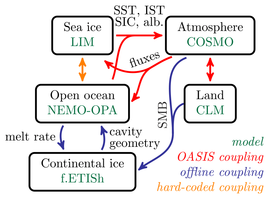
Figure 1 Fully coupled system submodel hierarchy. Each box represents an Earth system component and its corresponding model. The arrow colors distinguish the different coupling methods used, with legend given in the bottom right. “SST” stands for “sea surface temperature”, “SIC” – “sea-ice concentration”, “IST” – “ice surface temperature”, “alb.” – “albedo” and “SMB” – “surface mass balance”. Above, “NEMO-OPA” represents the open-ocean part of NEMO (i.e., NEMO without LIM). Although they are represented, the NEMO–COSMO exchanged fields are not detailed, as they have not been changed compared to existing settings.

3.1 COSMO–NEMO coupling interface

3.1.1 General description

In this section, we introduce the coupling interface between COSMO, the atmosphere model, and NEMO, the ocean–sea-ice model. We refer to “COSMO” (atmosphere model) instead of “CCLM²” (atmosphere–land model), since this coupling interface does not involve land processes. COSMO and NEMO are coupled online through OASIS3-MCT_2.0 (Valcke et al., 2013; Valcke, 2013). While this coupling interface has been built from pre-existing configurations involving these models (Van Pham et al., 2014; Will et al., 2017), our final setting includes several novel model developments which are described here. Figure 2 schematically represents this coupling interface.

Overall, NEMO sends COSMO surface values which are then used by COSMO to compute air–sea fluxes, eventually sent back to NEMO. The exchanged fields are detailed in Sect. 3.1.4. Spatial interpolations from one grid to the other are all performed bilinearly, except wind stresses which are interpolated bi-cubically to preserve curl. Despite being derived from the same initial f.ETISh geometry, the COSMO and NEMO continental masks may differ due to rounding effects at the coastline. In such cases, the nearest ocean neighbor is used to prevent COSMO from computing fluxes from land surface temperature with an ocean surface scheme, or NEMO from receiving fluxes that had been computed from the CLM land model.

The COSMO domain is smaller than NEMO's; hence, the ocean surface boundary condition is coupled to COSMO if possible; otherwise, outside of the COSMO domain, it is forced with atmospheric reanalyses (see Sect. 4.2 for more details). In order to avoid discontinuities and potential instabilities between both regimes, a linear transition over 20 NEMO grid points (the full grid being ≈600 grid points) is applied southwards from the limit of the COSMO domain. For the sake of consistency, the same reanalysis is used for forcing the COSMO lateral boundary condition and the extra-COSMO domain NEMO surface.

3.1.2 Timing strategy

The coupling frequency is set to the LIM time step (5400 s). Exchanged fields are time averaged over the past coupling window by OASIS. The coupling is asynchronous: NEMO receives surface fluxes from COSMO with a one-coupling-window delay, which is less than the typical forcing frequency used for running either model in stand-alone mode (in PARASO's case, 3 h). On the other hand, the surface values seen by COSMO are in real time, albeit originating from NEMO which had been constrained by time-staggered fluxes. At the end of a restart leg, the content of the coupler is written to disk in order to guarantee smooth restartability. During the first coupling window of the first restart leg, NEMO receives fluxes obtained from monthly averages of a previous coupled run.

3.1.3 Tiling representation in COSMO

The main coupling-related development lies in the implementation of tiling in COSMO to represent heterogeneous ocean surface cells, containing both open ocean and sea ice. Such methods have first been developed in land models (e.g., Koster and Suarez, 1992), then generalized to mixed surfaces (e.g., Best et al., 2004) and subsequently implemented in state-of-the-art surface modules (e.g., Voldoire et al., 2017). The standard COSMO configuration requires a single set of surface values over each cell, which is then used to compute vertical diffusion. The general strategy is to have COSMO compute a set of two tile-specific surface fluxes, from two distinct sets of surface properties corresponding to the open ocean and the sea ice. This is performed on all surface cells, regardless of the sea-ice concentration. The tile-specific fluxes are then sent to NEMO. The surface properties perceived by COSMO are degenerated from their tile-specific 2-fold values to a single set of values through pseudo-averaging. The pseudo-averaging consists in re-evaluating surface properties so that a given COSMO vertical column receives the concentration-wise average of the tile-specific fluxes it had computed. In that regard, the COSMO tiling implementation satisfies local air–sea energy conservation. Technical details on the pseudo-averaging operations are provided in Appendix D.

3.1.4 Exchanged fields

Table 2 lists the exchanged fields between NEMO and COSMO. Sea-ice surface properties are averaged over thickness categories so that only one set of sea-ice surface properties is read by COSMO, and only one set of air–sea-ice fluxes is sent from COSMO to NEMO. As described in Rousset et al. (2015), surface fluxes injected into the sea ice are redistributed so that LIM perceives distinct fluxes over each thickness category. With this redistribution, the net solar heat flux is the same as the one that would have arisen from a category-specific coupling and the net non-solar heat flux is a first-order development (w.r.t. surface temperature) of the category-specific case. While the wind stress computations do not take into account surface ocean currents or sea-ice velocities, their values above open ocean and sea ice are distinct as the surface roughness characterizations (and thus drag coefficients) differ. All heat fluxes are tile-specific and thus two-fold. Over each tile, the solar heat flux relies on its tile-specific albedo, with the sea-ice albedo taken as the average over ice-thickness categories from a parameterization depending on ice and snow thicknesses (Grenfell and Perovich, 2004; Brandt et al., 2005). The tiled non-solar heat fluxes contain net longwave (including direct downward atmosphere and upward surface contributions), sensible and latent contributions. The turbulent heat fluxes (sensible and latent heat) depend on surface properties, and tile-specific turbulent heat transfer coefficients are evaluated from a turbulent kinetic energy (TKE)-derived scheme (Doms et al., 2018). The latent heat fluxes are used for the diagnostic of sea-ice sublimation and open-ocean evaporation. Sea-ice sublimation is permitted but solid condensation is not: in other words, over sea ice, downward latent heat can only be negative (i.e., it is set to zero if the surface scheme assumes it is positive). Rainfall is injected as freshwater at sea surface temperature; over sea ice, it is assumed to immediately run off to the open ocean. Over sea ice, solid precipitation contributes to snow accumulation; over the open ocean, it is assumed to immediately melt, and the corresponding latent heat is removed from the local ocean surface cell. The computation of the surface temperature over sea ice requires the non-solar heat flux sensitivity (i.e., its derivative w.r.t. surface temperature) to ensure numerical stability, since the sea-ice surface temperature may significantly evolve within a coupling window (Iovino et al., 2013). The sensitivity estimate is local both time- and space-wise: it includes the temperature's influence on surface moisture but assumes the heat transfer coefficient to be constant (which is a simplification). Fluxes over sea ice are systematically computed and sent over all ocean cells using the last known (initial) sea-ice surface properties in the event that no sea ice is currently (has ever been) present in the category. This is carried out in the event that sea ice appears, through advection or thermodynamics, over one grid cell within a coupling window.

Table 2 NEMO–COSMO list of exchanged variables.

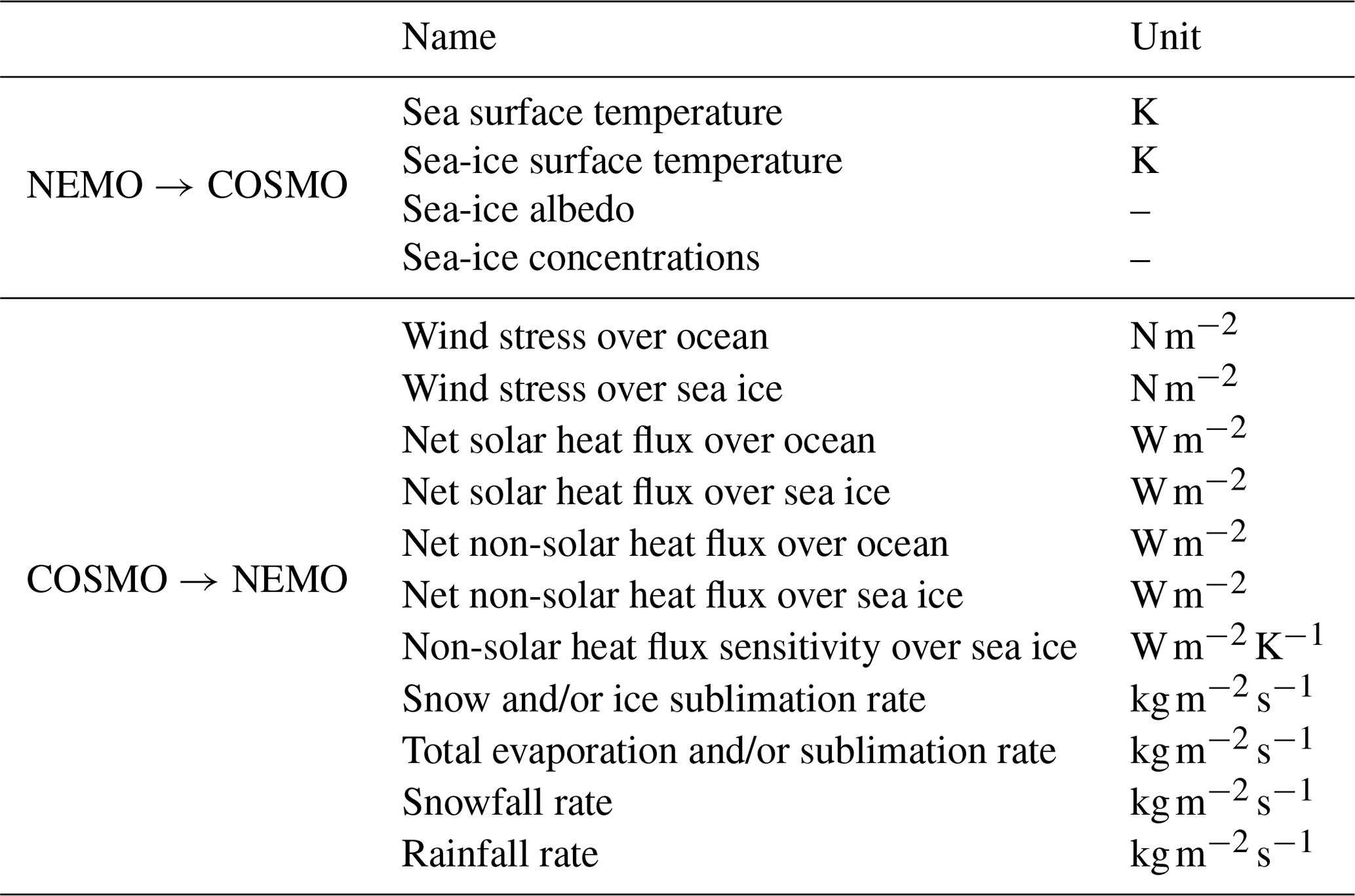
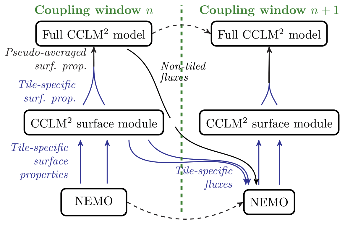
Figure 2 COSMO–NEMO coupling interface diagram for two coupling windows. Full blue (black) arrows correspond to exchange of tile-specific (non-tiled) fields. The thick dashed vertical line delimits the transition from one coupling window to the next one. NEMO sends tile-specific surface properties to the COSMO surface module, which are used to compute tile-specific fluxes. These fluxes are then (i) sent back to NEMO on the next coupling window (hence NEMO getting delayed fluxes); (ii) pseudo-averaged to be injected into the COSMO dynamics. In addition, non-tiled fluxes (e.g., precipitation) are also sent from COSMO to NEMO. For the sake of readability, the incoming (outgoing) fluxes from coupling window n−1 (to coupling window n+2) are not represented.

3.2 NEMO–f.ETISh coupling interface

3.2.1 General procedure

Figure 3 schematically represents the NEMO–f.ETISh coupling interface. Like most idealized and realistic settings (e.g., Timmermann and Goeller, 2017; Favier et al., 2019), the coupling between NEMO and f.ETISh is offline. NEMO runs first for a coupling time window, sending f.ETISh monthly time series of ice-shelf melt fluxes (both melt and refreezing are permitted). While NEMO computes both mass and latent heat fluxes related to the ice-shelf melting and incorporate them as ocean boundary conditions at the ice-shelf base, only the mass flux is sent to f.ETISh. The grounding line (including cavity opening and closing) and ice thickness are evolving freely with the minimum bound on ice-shelf thickness of 11 m (very thin compared to typical values) to keep the ice-shelf extent constant, so that the PARASO land–sea mask does not evolve. Afterwards, NEMO waits while f.ETISh runs for the same coupling window, including the received melt rates as a boundary condition. After this, f.ETISh provides NEMO an updated ice-sheet geometry. NEMO then uses this new ice-shelf draft dataset starting from the beginning of the next coupling window. This process is iteratively repeated over each coupling window until the end of the simulation.

Figure 3 NEMO–f.ETISh coupling procedure. The box represents the coupling loop (one iteration per NEMO–f.ETISh coupling window). Colored arrows represent the data exchange between NEMO and f.ETISh. The NEMO spinup run is used as initial conditions for the first NEMO leg only.

3.2.2 Timing strategy

Our implementation is using a collaborative job submission script manager for NEMO called Coral. The coupling frequency can be changed, as long as it is (all conditions must be met)

• an integer number of months;

• a multiple of the NEMO restart length; and

• a divisor of the total experiment length.

NEMO always provides monthly subshelf melt rates to f.ETISh to include seasonality regardless of the coupling frequency and receives the simulated ice-shelf draft from f.ETISh at the end of the coupling step. For the results presented in Sect. 5, the NEMO-f.ETISh coupling frequency has been set to 3 months. This was chosen so that our relatively short (2-year) experiments can include a few ocean–ice-sheet coupling occurrences.

3.2.3 Exchanged fields

f.ETISh sends NEMO

• is_ice, a Boolean variable distinguishing ice-sheet columns (true for ice shelves and grounded ice) from ocean ones (true for open-ocean);

• is_dry, a Boolean variable distinguishing dry columns (true for grounded ice) from wet ones (true for ice-shelf cavities and open-ocean);

• ice surface elevation; and

• water column thickness.

These fields are then interpolated with a conservative method. The resulting columns are treated differently according to the interpolated Boolean variable values with a 50 % threshold, as described in Fig. A2. With this procedure, grounding-line displacement is theoretically bounded by the NEMO grid southern limits, which, for PARASO, covers most of Antarctica (see the NEMO grid imprint in Fig. 4).

NEMO sends f.ETISh monthly mean subshelf melt rates as freshwater mass fluxes $\left[\mathrm{kg}{\mathrm{m}}^{-\mathrm{2}}{\mathrm{s}}^{-\mathrm{1}}\right]$, which are converted to ice equivalent melt rates [m yr⁻¹] by applying an ice density of ρ_ice=917 kg m⁻³. The mask discrepancies between NEMO and f.ETISh (e.g., arising from the NEMO-specific criteria for opening columns described in Sect. 4.1.2) are dealt with on a cavity-by-cavity basis. If a f.ETISh cavity is at least partly covered by NEMO, the NEMO melt rates are interpolated bilinearly (applied for about 84 % of all ice-shelf grid cells in f.ETISh) with potential nearest-neighbor extrapolation to cover f.ETISh cavity columns which correspond to closed columns in NEMO (applied for about 15 % of all ice-shelf grid cells). Only a few very small and dynamically insignificant ice shelves are not represented in NEMO, summing up about 1 % of all ice-shelf grid cells in f.ETISh. Melt rates of cavity columns in NEMO which correspond to grounded ice or open ocean in f.ETISh are disregarded (applicable for about 2.5 % of the ice-shelf area in NEMO). The distribution between those procedures (84 % interpolation, 15 % extrapolation and 1 % not represented in NEMO) is dominated by the different grids of NEMO and f.ETISh and stays almost constant even for longer runs (a few decades; not shown here); the coupling frequency only has a very minor influence on this phenomenon.

3.2.4 Procedure for opening and closing cavity cells in NEMO

After each ocean–ice-sheet coupling episode, NEMO uses the post-processed updated f.ETISh geometry as its new subshelf cavity geometry. In PARASO, the post-ice-sheet-coupling NEMO procedure of Smith et al. (2021) is employed. For the sake of completeness, its main steps and characteristics are briefly described below.

The geometry constraints described in Table 1 are enforced at each coupling time step. The sea surface height, temperature and salinity of a newly opened ocean column are extrapolated from their neighboring cells (Favier et al., 2019). The extrapolation procedure is repeated 100 times, which yields a smoothing effect over potentially large new openings. The initial current velocities of new cells are set to zero. On all modified columns (thinned or thickened), a horizontal divergence correction is applied in order to avoid spurious vertical velocities.

Two minor caveats keep this post-coupling procedure from being conservative. First, artificial mass and heat fluxes are brought into (taken from) the ocean upon cell opening (closing). For example, when ice-sheet geometry changes lead to a NEMO cell opening (closing), the corresponding volume and internal energy are added into (extracted from) the ocean. These fluxes are not related to ice-shelf melting and refreezing, whose associated mass and heat fluxes are already included as ocean boundary conditions at the shelf base and at each NEMO time step by its cavity module, regardless of whether ocean–ice-sheet coupling is activated (see Sect. 2.2.2). Second, the divergence correction applied after each ocean–ice-sheet coupling yields phantom current velocities into (out of) the grounded ice sheet upon cell opening (closing), which implies minor artificial ocean mass and internal energy changes. Since PARASO is a regional configuration with desired simulation times of a few decades at best, this lack of conservation has been deemed acceptable.

Geometry variations lead to spurious barotropic currents dissipating over the first few days following a mesh update. Practically, this implies that the coupling numerical stability is conditioned by the amplitude of the geometry variations through one update. However, we have observed that enforcing the NEMO cavity geometry constraints described in Table 1 keeps critical numerical instabilities from arising, even with yearly coupling windows (not shown here).

3.3 CCLM²–f.ETISh interface

The exchange between CCLM² and f.ETISh runs one way (from CCLM² to f.ETISh) and performed offline. CCLM² runs for one coupling time window, sending f.ETISh monthly time series of surface mass balance (SMB), which here boils down to solid precipitation minus surface sublimation. The SMB is converted from m yr⁻¹ by using the reference ice density of ρ_ice=917 kg m⁻³. Interpolations between the CCLM² and f.ETISh grids are performed bilinearly. For the sake of simplicity, the coupling window partitioning for the CCLM²–f.ETISh interface is the same as the NEMO–f.ETISh one, and the workflow is managed with the same job submission tool (Coral).

The SMB received from CCLM² is included within the surface boundary condition of f.ETISh. However, variations in ice-sheet surface elevation are not sent back to CCLM², which is a limitation of PARASO, and the reason why this “coupling” procedure is referred to as “one way”. It should however be stressed that at the timescales PARASO has been developed for (decadal at the longest), variations in Antarctic surface topography are negligible.

4 The PARASO configuration

4.1 General description and geometry

In this subsection, we detail each subcomponent of the PARASO configuration. Table 3 contains a brief, cross-model overview, and Fig. 4 shows and compares each model's configuration geometry.

Table 3 Summary of PARASO model setups. “res.” stands for “resolution”.

^* Reference elevation model of Antarctica (Howat et al., 2019).

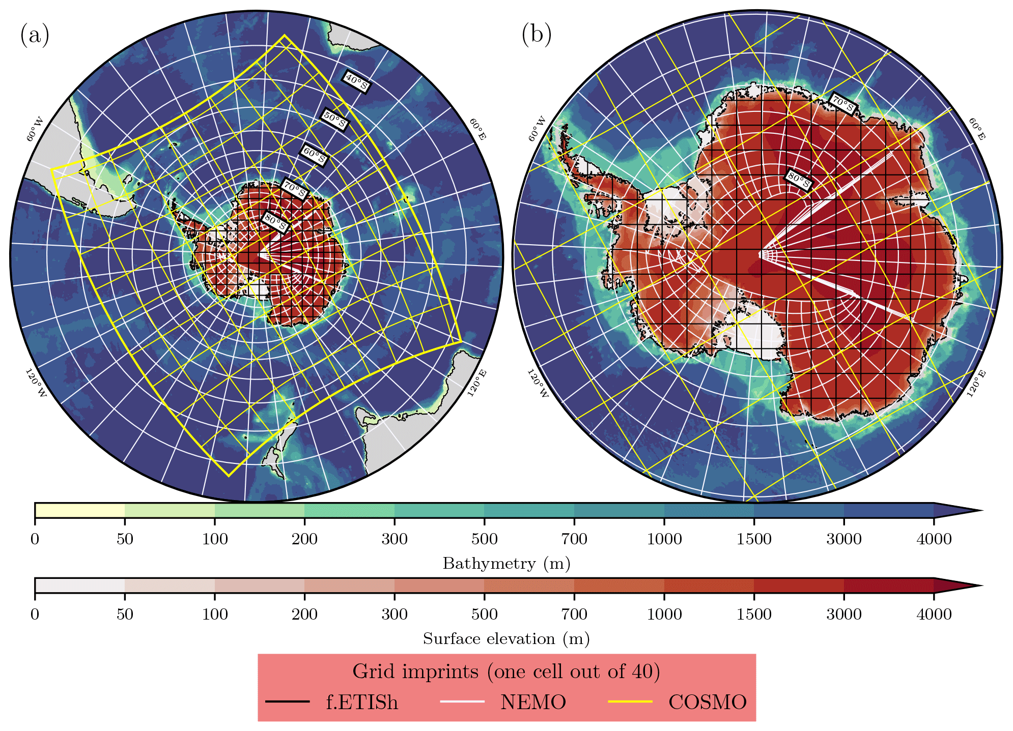
Figure 4 PARASO configuration geometry over (a) the full NEMO domain (cut at 30^∘ S) and (b) Antarctica. The two color maps indicate the bedrock bathymetry and the ice surface elevation (Morlighem et al., 2020) over Antarctica (note the nonlinear scale). The lines represent the f.ETISh, NEMO and COSMO grids (for the sake of readability, not all cells are drawn).

4.1.1 f.ETISh configuration

The f.ETISh model is run on a regular polar stereographic grid of 701×701 grid points centered around the South Pole, with a horizontal resolution of 8 km. The f.ETISh time step is $\mathrm{1}/\mathrm{60}$ yr. The domain encompasses the continental shelf and shelf break, which limits the maximum possible extension of the ice sheet. Bedrock topography, bathymetry, observed ice thickness and grounding-line position are taken from BedMachine Antarctica (Morlighem et al., 2020). This dataset, originally at a 500 m spatial resolution, has been resampled to the f.ETISh 8 km grid using a low-pass filter. Data were subsequently corrected to ensure grounded ice being actually grounded and floating ice actually floating. The initial ice-sheet geometry for the PARASO setting is derived from the initialization and relaxation described in Sect. 4.3. For the PARASO configuration, iceberg calving has been omitted (but they are part of the NEMO forcing; see Sect. 4.1.2). The land-ice extent is kept constant as the NEMO-COSMO interface has not been designed to deal with an evolving land–sea mask. This is one clear limitation which prevents PARASO from being relevant at multidecadal and longer timescales: in that case, the rapidly melting ice-shelf cavities would be carved from below and reach an unrealistically thin shape. Growing ice shelves are cut off at the calving front derived from BedMachine Antarctica (Morlighem et al., 2020), but the equivalent iceberg melt flux is not injected into NEMO (an external iceberg melt dataset is used; see Sect. 4.2.2). Moreover, in accordance with the constraints listed in Table 1, shrinking ice shelves cannot become thinner than 11 m (≈10 m draft, which is considerably smaller than typical draft values).

4.1.2 NEMO configuration

The NEMO PARASO setup is derived from the GO7 configuration described in Storkey et al. (2018). The ocean grid is ePERIANT025, which includes the southernmost ice-shelf cavities (Mathiot et al., 2017). With a single lateral ocean boundary at 30^∘ S, NEMO has the widest spatial coverage of all PARASO subcomponents. The effective ocean model resolution decreases from 24 km at the 30^∘ S boundary to 14 km at 60^∘ S, eventually reaching 3.8 km in its southernmost cells (in the Ross cavity at approximately 86^∘ S). The vertical discretization includes 75 levels with thickness increasing from 1 m at the surface to ∼200 m at depth. The NEMO and LIM time steps are 900 and 5400 s, respectively. The Antarctic continental shelf bedrock bathymetry is taken from BedMachine Antarctica (Morlighem et al., 2020) with a linear transition to ETOPO1 (Amante and Eakins, 2009) to cover the remaining PARASO domain (northwards from roughly 63^∘ S). For numerical stability, a minimal ocean depth of 20 m is imposed. The Antarctic surface continental mask is constant time-wise (calving is not permitted) and taken from the ice-sheet geometry obtained from the initial f.ETISh run described in Sect. 4.3. Ice-shelf cavities are opened to ocean circulation (Mathiot et al., 2017) with three geometrical constraints balancing physical realism and numerical stability (see Table 1):

1. the minimal ice-shelf draft and water column height are set to 10 and 50 m, respectively;

2. columns within ice-shelf cavities must have at least two vertical levels to allow overturning circulation;

3. subglacial lakes (i.e., floating continental ice surrounded by grounded ice and separated from the ocean), ice-shelf crevasses and “chimneys” (vertical ocean segments surrounded by ice in all directions and connected to the cavity) are removed by NEMO (i.e., they are artificially filled with ice from their nearest-neighbor ice-shelf column).

Parameters enforcing these constraints are also listed in Table 1. At the depths of the ice-shelf cavities, the vertical resolution roughly ranges from 10 to 150 m (but we remind the reader that partial cells are used).

4.1.3 CCLM² configuration

In PARASO, the COSMO rotated latitude–longitude grid has a horizontal resolution of 0.22^∘ (approximately 25 km at the Antarctic coastline), covering the whole Antarctic ice sheet as well as a significant part of the Southern Ocean, with the northern boundary located between 50 and 40^∘ S. The terrain-following vertical discretization has 60 levels. The lowest model level is at 5 m height and cell thicknesses span from 10 m at the bottom to 1000 m at the top. The COSMO and CLM time steps are 90 and 3600 s, respectively. The COSMO-CLM coupling is performed at every CLM time step (3600 s frequency).

4.2 External forcing

4.2.1 f.ETISh forcings

The only f.ETISh forcings are subshelf melt rates and SMB, which are provided by NEMO and CCLM² (respectively) and updated at every coupling window.

4.2.2 NEMO forcings

Over the ocean surface located outside of the CCLM² spatial coverage, the NEMO surface is forced with fluxes computed by the CORE bulk formula (Large and Yeager, 2004), using the ERA5 reanalysis as atmosphere input (Hersbach et al., 2020). The resulting air–sea fluxes are different from the ones that the COSMO surface scheme (prescribed over the coupled part of the domain) would have provided. This limiting trade-off is related to the nature of the COSMO surface scheme, requiring model-specific atmospheric input fields which are typically not distributed in reanalyses (e.g., the TKE at the lowest two atmospheric levels). At its 30^∘ S lateral open-ocean boundary, NEMO is constrained with the NEMO-based ORAS5 ocean reanalysis (Zuo et al., 2019) at monthly frequency. The lateral boundary condition is enforced with a radiation scheme (see Eq. 9 in Flather, 1994) for 2-D dynamics (sea surface height and barotropic velocities) and a flow relaxation scheme for the baroclinic velocities, temperature and salinity. A constant $\mathrm{86.4}\times {\mathrm{10}}^{-\mathrm{3}}$ W m⁻² geothermal flux is imposed at the bottom of the ocean (Stein and Stein, 1992). River runoff is adapted from Dai and Trenberth (2002) and prescribed as a climatological dataset (Bourdallé-Badie and Treguier, 2006). While icebergs are not dynamically simulated, their freshwater melt input is injected as additional runoff from an interannual dataset obtained from a previous iceberg-including NEMO simulation covering 1979 to 2015 (Marsh et al., 2015; Merino et al., 2016; Jourdain et al., 2019). Buoyant plume mixing resulting from runoff is parameterized with enhanced mixing in the shallowest 10 m, over the river deltas and on a stripe between 20 and 200 km from the Antarctic coast (where most of the iceberg melting occurs). Enhanced mixing is excluded in the direct vicinity of the coast to avoid interferences with ice-shelf meltwater (Nicolas C. Jourdain, personal communication, 2019). No salinity restoration is applied.

4.2.3 CCLM² forcings

At its lateral boundaries, COSMO is relaxed to ERA5 using a one-way interactive nesting based on Davies (1976). This consists in defining a relaxation zone where the internal COSMO-CLM solution is nudged against the external ERA5 solution. Within this zone, the variables of the driving model are gradually combined with their corresponding variables in COSMO-CLM by adding a relaxation forcing term to the tendency equations that govern their evolution. The attenuation function which specifies the lateral boundary relaxation inside the boundary zone has a tangent hyperbolic form (Kållberg, 1977). The width of the relaxation layer is set to 220 km, which corresponds to approximately 10 times the typical cell size. More information about the one-way nesting can be found in the COSMO documentation (Doms and Baldauf, 2018). The boundary forcings (as well as the initial conditions) for the COSMO model have been prepared at discrete time intervals using the interpolation program INT2LM (Schättler and Blahak, 2013). The interval between two consecutive sets of boundary data (frequency of the lateral forcing) is 3 h. Within this time interval, boundary values are interpolated linearly in time. The 3-D atmospheric variables for COSMO are wind speeds (zonal and meridional), air temperature, pressure deviation from a reference pressure (1000 hPa at sea level), specific water vapor content, specific cloud water content and specific cloud ice content. No spectral nudging has been applied to the upper atmosphere model levels to preserve the CCLM² atmosphere dynamics. A sponge layer with Rayleigh damping in the upper levels of the model domain is activated in order to avoid artificial reflections of gravity waves. A cosine damping profile with maximum damping at the top and zero damping at the base of the sponge layer (11 000 m elevation) is applied.

4.3 Initialization

Prior to running the fully coupled system, a f.ETISh stand-alone initialization and relaxation run (see Sect. 4.3.1) is performed in order to generate a steady Antarctic ice-sheet state used as an initial geometry for all three subcomponents (see Fig. 4).

4.3.1 f.ETISh initialization

The f.ETISh model initialization is derived from an adapted iterative procedure based on Pollard and DeConto (2012) to fit the model as close as possible to present-day observed thickness (BedMachine Antarctica; Morlighem et al., 2020) and flow field by iteratively updating local basal friction coefficients (Pattyn, 2017). The method has been further optimized to enhance convergence (Bernales et al., 2017). In addition to Pollard and DeConto (2012), we also implemented a regularization term that uses a 2-D Gaussian smoothing kernel to filter out high-frequency noise in the basal sliding coefficients. For the initialization, f.ETISh is run with reduced complexity, using the SIA for the evolution of the grounded ice sheet, thereby keeping ice shelves in the observed geometry. Optimized basal sliding coefficients and steady-state modeled geometry for the Antarctic ice sheet were obtained after a forward-in-time integration of 60 000 yr with thermomechanical coupling. The initial temperature field (prior to that forward run) is derived from a steady-state temperature solution based on the present-day surface temperature, surface mass balance and geothermal heat flux. The latter is based on the seismic-based dataset due to Shapiro and Ritzwoller (2004). For the relaxation, ice shelves are allowed to evolve and the hybrid shallow-shelf–shallow-ice approximation (HySSA; Bueler and Brown, 2009) is used to obtain the velocity field. The applied subshelf melt rates are taken as the constant (time-wise) 1984–1993 mean from a NEMO stand-alone run. The PARASO setting of f.ETISh (e.g., constant calving front; compare Sect. 4) is run for 20 years to gain the relaxed geometry (see Fig. A8), representing the initial geometry for the PARASO configuration. The duration of 20 years is the result of a trade-off between gaining quasi-steady-state ice-flow velocities and reducing the ice-shelf thinning during the relaxation. For the initialization and the relaxation, f.ETISh is forced by a constant surface temperature and SMB climatology provided by AEROCLOUD, a previous CCLM² stand-alone experiment (Souverijns et al., 2019).

4.3.2 NEMO initialization

The ocean is initialized from a 1-year spinup run performed with NEMO stand-alone, using forcings corresponding to the year 1999, to be as consistent as possible with ones used in PARASO: ORAS5 for the ocean lateral boundary condition and ERA5 for the ocean–atmosphere surface. As already mentioned in Sect. 4.2.2, the resulting fluxes are not identical to the coupled ones since the NEMO coupled (COSMO surface scheme) and stand-alone (CORE) bulk formulae differ. For the spinup, the 3-D initial conditions for temperature and salinity are taken from the final 10-year climatology of a cavity-including 40-year NEMO stand-alone run, so that the spinup is in equilibrium, in terms of both dynamics and thermodynamics. This allows PARASO to start from an upper-ocean state roughly matching the CCLM² initialization, which is also based on ERA5, up to the limits permitted by the differences in air–sea bulk formulae.

4.3.3 CCLM² initialization

The land and ice masks used by CCLM² to determine the fraction of land vs. ocean and land ice vs. ice-free areas are calculated on the CCLM² grid based on the geometry provided by f.ETISh, so that the geometry of the fully coupled setup is consistent from one subcomponent to another.

COSMO 3-D fields are initialized from the ERA5 atmospheric reanalysis (Hersbach et al., 2020). The CLM model starts from hard-coded initial conditions (Oleson et al., 2013); hence, the atmosphere–land system does not start from equilibrium. The visible and near-infrared albedos for glacier ice are respectively set to 0.80 and 0.55. Glacier temperatures are initialized at −23.15 ^∘C. The overlying snowpack is modeled with up to five layers, depending on the total snow depth. At the initialization, five layers are used to represent a snow water equivalent (SWE) of 1 m (the maximum snow depth in SWE), which corresponds to a 4 m thick snow layer for a bulk snow density of 250 kg m⁻³. The snow liquid water and ice content for layer i=1 to 5 is set to $w_{\mathrm{liq},i}=\mathrm{0}$ kg m⁻² and $w_{\mathrm{ice},i}=\mathrm{\Delta }{z}_i{\mathit{\rho }}_{\text{sno}}$ kg m⁻², respectively. Although a 1 m SWE snowpack is too small to fully represent the firn layer, which can extend to more than 100 m in Antarctica (van den Broeke et al., 2009), Souverijns et al. (2019) showed that this choice can lead to a decent SMB representation in CCLM² as long as the adaptations from van Kampenhout et al. (2017) are included in the CLM snow module (except for the snowpack depth). For future PARASO-related work, keeping a maximum snow depth of 1 m is also convenient to limit the spinup phase of the snowpack to a few years at most. Multiple surface datasets are also required to initialize CLM. They are listed in Table 2.5 of Oleson et al. (2013) and come from a variety of sources. Depending on the domain (location, resolution), datasets can be downloaded and regridded on a case-by-case basis using the CESM tools (the procedure is described in chap. 1 of Vertenstein et al., 2013). Note that one specificity of PARASO lies in the modifications of the land mask and mean elevation, carried out to be consistent with the f.ETISh relaxation run (see Fig. 5). In particular, the ice-shelf surface elevation is represented, while the original CESM data simply assume all ice shelves to be exactly at sea level.

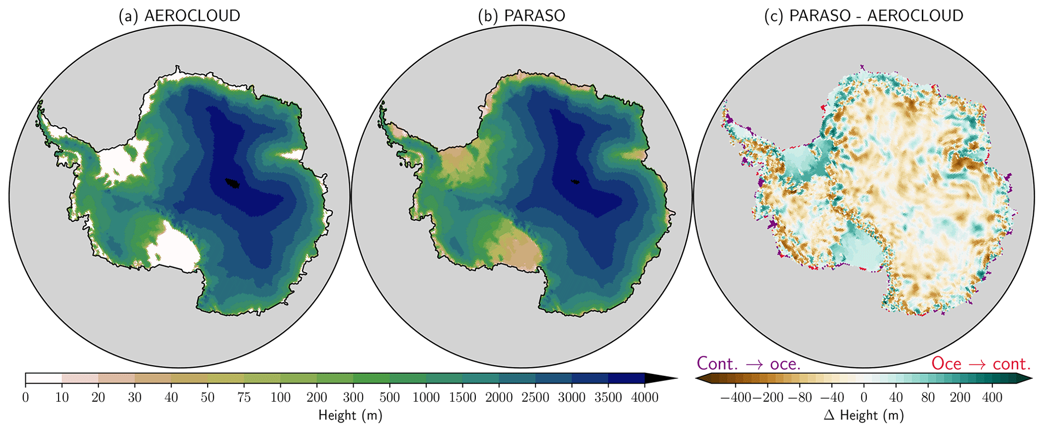
Figure 5 Surface elevation for (a) a previous CCLM² stand-alone model configuration (AEROCLOUD), (b) PARASO and (c) their absolute difference (PARASO–AEROCLOUD). Note that all color scales are nonlinear. In panel (c), nodes that change nature, from AEROCLOUD land to PARASO ocean (AEROCLOUD ocean to PARASO land), are displayed with purple (red) shadings.

5 Results

In this section, diagnostics from a 2-year (2000–2001) PARASO experiment are presented and evaluated. Unless explicitly specified otherwise, the results shown are taken from the second simulated year (2001) in order to limit the influence of the initialization.

PARATMO, a CCLM² stand-alone experiment whose atmospheric experimental design is identical to PARASO's, serves as a comparison basis for atmospheric results. PAROCE is an analogous twin ocean experiment. In Sect. 5.3, PARASO is also compared to AEROCLOUD (a previous CCLM² stand-alone experiment detailed in Souverijns et al., 2019), which does not share the same experimental design. Moreover, three f.ETISh stand-alone experiments are performed. These experiments only differ in their forcing, which correspond to coupled fields in PARASO, and have been specifically designed to gradually investigate the impact of the two coupling interfaces involving f.ETISh. PARCRYO^CTRL is forced with the constant SMB used during the initialization (provided by AEROCLOUD; see Sect. 4.3.1), and no subshelf melt is applied. It serves as a comparison basis since the CCLM² inputs to f.ETISh are from AEROCLOUD rather than any PARASO-like experiments, and no input whatsoever from NEMO is included. PARCRYO^SMB also does not apply subshelf melt but is forced with monthly SMB from PARATMO, to isolate the effects of the CCLM²–f.ETISh coupling interface from the NEMO–f.ETISh one. Finally, PARCRYO is forced with monthly SMB from PARATMO and monthly subshelf melt rates from PAROCE. It includes inputs from both CCLM² and NEMO but does not account for ocean–ice-sheet feedback as PARASO does through the NEMO–f.ETISh coupling interface. A summary of all experiments designed for this study and used for diagnostics is provided in Table 4.

Table 4 List of experiments from which the presented diagnostics are derived. Besides the presence (or lack thereof) of model components and coupling interfaces, all experiments share the same design and cover the 2000–2001 period.

^* Same experimental design as PARASO except for the surface flux tiling which has not been implemented in the CCLM² stand-alone experiment.

The PARASO biases are more generally discussed and put into perspective in Sect. 6. Computational aspects related to PARASO are briefly covered in Appendix B. PARASO-specific tunings used for obtaining a realistic sea-ice seasonal cycle are described in Appendix E.

5.1 Ice sheet and ice shelves

Figure 6 displays the subshelf melt rates for PAROCE and PARASO in different regions. Both experiments' regional melt rate patterns agree relatively well with each other (Fig. 6b–e), but the total melt of PARASO is significantly increased in the Weddell (+31 %), Indian Ocean (+85 %) and West Pacific (+162 %) sectors (see Fig. 6a–c and f) due to the warmer and more saline eastern Antarctic surface water in PARASO (see Figs. 6g, 9k, m and 10k, m). However, the West Antarctic melt rates remain of similar magnitude from PAROCE to PARASO (−9 % in the Amundsen Sea and −16 % in the Bellingshausen Sea; see also Fig. 6a and d–e). This adds up to a 2001 average circumpolar PARASO melt rate of 1103 Gt yr⁻¹, +33 % compared with PAROCE's 829 Gt yr⁻¹. Compared to observed ice-shelf melt rates from Rignot et al. (2013) and Adusumilli et al. (2020), both experiments underestimate subshelf melt. While the simulated melt rates for the Ross and Weddell seas match observations, the melt for the West Pacific sector, Bellingshausen Sea and Amundsen Sea in particular, is considerably lower (Fig. 6a). The underestimated melt rates likely stem from the initial PARASO ice-shelf geometry arising from the f.ETISh initialization (see Sect. 4.3 and Fig. A8), which differs more from the observed geometry in western Antarctica compared to the other sectors. A similar NEMO stand-alone run (not shown here) with an observation-based ice-sheet geometry (from BedMachine Antarctica, Morlighem et al., 2020) provides significantly larger melt rates in those regions, in better agreement with Rignot et al. (2013) and Adusumilli et al. (2020). These results support that the geometry is a main driver of the observed melt biases. The importance of cavity geometry on simulated melt rates has already been emphasized by previous studies (Schodlok et al., 2012; Rosier et al., 2018; Goldberg et al., 2019; Brisbourne et al., 2020; Goldberg et al., 2020; Wei et al., 2020).

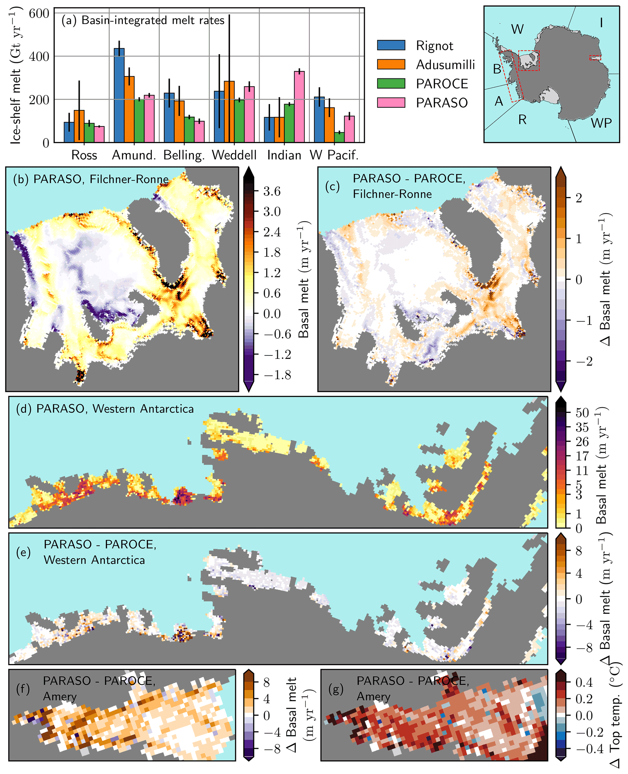
Figure 6 (a) Total ice-shelf melt rate over all sectors (see initials on indicative map) from observations (Rignot et al., 2013, and Adusumilli et al., 2020), PAROCE and PARASO. For observations, error bars correspond to measures uncertainties; for PAROCE and PARASO, to intra-annual STD. (b–c) Zoom-in on the Filchner–Ronne cavity for (b) PARASO (negative values indicate ice-shelf refreezing) and (c) PARASO–PAROCE differences (positive values indicate stronger PARASO melting). (d–e) Zoom-in for the western Antarctic sector for (d) PARASO (note the nonlinear color map scale) and (e) PARASO–PAROCE differences. (f–g) Zoom-in on the Amery Ice Shelf for (f) melt rate and (g) top conservative temperature PARASO–PAROCE differences. All simulation diagnostics are averaged over 2001 (second simulated year).

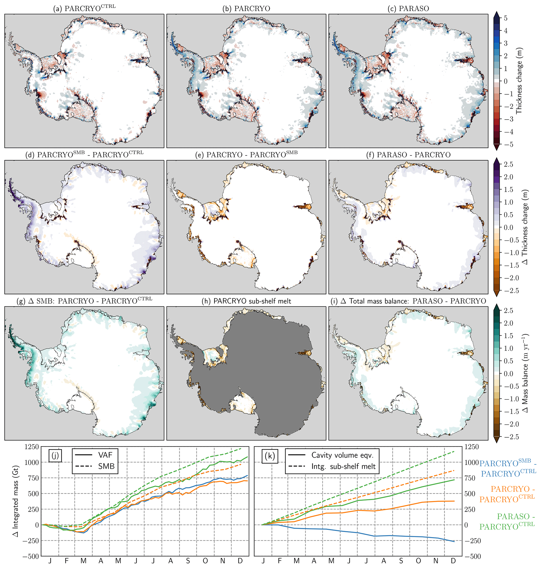
Figure 7 (a–c) Ice-thickness change during the year 2001 for (a) PARCRYO^CTRL, (b) PARCRYO and (c) PARASO. (d–f) Difference of the ice-thickness change between (d) PARCRYO^SMB and PARCRYO^CTRL, (e) PARCRYO and PARCRYO^SMB and (f) PARASO and PARCRYO. (g) Difference between the mean SMB applied for PARCRYO (SMB based on PARATMO) and for PARCRYO^CTRL (SMB from initialization run based on AEROCLOUD). (h) Mean subshelf melt rates (from PAROCE) applied for PARCRYO (equivalent to Δ (PARCRYO–PARCRYO^CTRL) since no subshelf melt is applied in PARCRYO^CTRL). Out of consistency with panel (g), negative (positive) values indicate melting (refreezing). (i) Difference of the total mass balance between the coupled PARASO and the stand-alone PARCRYO experiment. (j) Change of the volume above floatation (VAF) and the integrated SMB and (k) change of the cavity volume and the integrated subshelf melt. (j–k) PARCRYO^SMB, PARCRYO and PARASO are plotted as anomalies compared to PARCRYO^CTRL. In panel (j), the PARCRYO^SMB SMB anomalies are not plotted as they are identical with that of PARCRYO, by design. In panel (k), the PARCRYO^SMB integrated subshelf melt anomalies are not plotted as no melt is applied for that experiment. All results are from 2001 (second simulated year).

Figure 7 compares PARASO and the PARCRYO experiments, corresponding uncoupled stand-alone f.ETISh simulations for different forcings (see Table 4). Overall, PARCRYO and PARASO display similar behavior across most coastal regions, and in particular the Antarctic Peninsula, with a moderate grounded ice-thickness increase up to a few meters (Fig. 7b–c). That thickening also occurs for PARCRYO^SMB (Fig. 7d) and agrees well with the differences between the forcing SMB datasets (Fig. 7g). PARACRYO^SMB and PARACRYO apply the SMB from PARATMO, while PARACRYO^CTRL is forced by the SMB based on AEROCLOUD that has been used for the f.ETISh initialization (see Sect. 4.3.1). The direct comparison of PARCRYO and PARASO (see Fig. 7f) reveals a slightly larger thickening of the grounded ice in coastal areas for PARASO. This is in accordance with the increased SMB for those regions provided by CCLM² in PARASO (Fig. 7i). Figure 7j also emphasizes the relationship between the SMB forcing and the thickness evolution of the grounded ice. While the SMB is quite constant for the first 2 months, the change in ice volume (VAF) can be attributed to the dynamical response of the modeled ice sheet, as it has probably not reached a steady state. Furthermore, the presented mass changes (ΔVAF) are the mass changes due to the forcing as the VAF of the control run has been subtracted. PARCRYO and PARCRYO^SMB, which are forced by the identical SMB dataset (from PARATMO), show a very similar evolution of the grounded ice (Fig. 7e), while the change of the volume above floatation (VAF) for PARASO clearly follows the enhanced SMB. A more detailed discussion of the differences between AEROCLOUD, PARATMO and PARASO can be found in Sect. 5.3. Other ice-thickness changes occur at the grounding line (Fig. 7a–c), as the relatively coarse resolution and numerical uncertainties of the grounding-line flux induce small oscillations between neighboring grid cells in the grounding-line position. Furthermore, the experiments show a thickening of many narrow ice streams (e.g., Pine Island Glacier, Byrd Glacier, Rutford Ice Stream), and only Thwaites Glacier shows significant grounded ice mass loss (Fig. 7a–c). The suspicious thickening is due to both the limited resolution and the initialization (see Sect. 4.3.1) and causes a certain model drift.

The forcing with subshelf melt, which has only been applied for PARCRYO (subshelf melt from PAROCE) and PARASO, has a very limited effect on the grounded ice on the short evaluation period of 1 year but clearly affects the ice shelves (Fig. 7e). The ice shelves show a moderate thinning of up to a few meters almost everywhere, except in the Bellingshausen Sea, where substantial ice-shelf thickening occurs (Fig. 7b–c), as the increase of the SMB compared to PARCRYO^CTRL exceeds the applied subshelf melt (Fig. 7g and h), while for the other regions the subshelf melt is the dominating forcing for the ice shelves. Figure 7k illustrates the influence of the different SMB forcing on the ice shelves. The enhanced SMB of PARCRYO^SMB compared to PARCRYO^CTRL leads to a decrease of the cavity volume and hence ice-shelf thickening. Figure 7k also exhibits enhanced ice-shelf thinning (stronger cavity volume increase) of PARASO compared to PARCRYO, following the increased subshelf melt of PARASO. The increased ice-shelf thinning of PARASO mainly occurs across the East Antarctic ice sheet (Fig. 7f) and is in accordance with the increased subshelf melt of PARASO, which also mainly affects the East Antarctic ice shelves (Figs. 6a and 7i).

In terms of ice–ocean coupling, the ice sheet behaves very similarly for both coupled and uncoupled experiments (PARASO and PARCRYO, respectively), and their differences are explained by discrepancies in ice-sheet forcing (SMB from CCLM², subshelf melt rates from NEMO). No biases or additional noise due to the coupling itself have been found for the ice-sheet model. It should be kept in mind, however, that both simulations cover only 2 years, which is a short period for the relatively slow (e.g., in comparison with the ocean and atmosphere) ice-sheet system.

5.2 Ocean and sea ice

In this section, we compare PARASO results to observations as well as to PAROCE, a NEMO stand-alone experiment forced by ERA5, with the same experimental design (except the coupling; see Table 4).

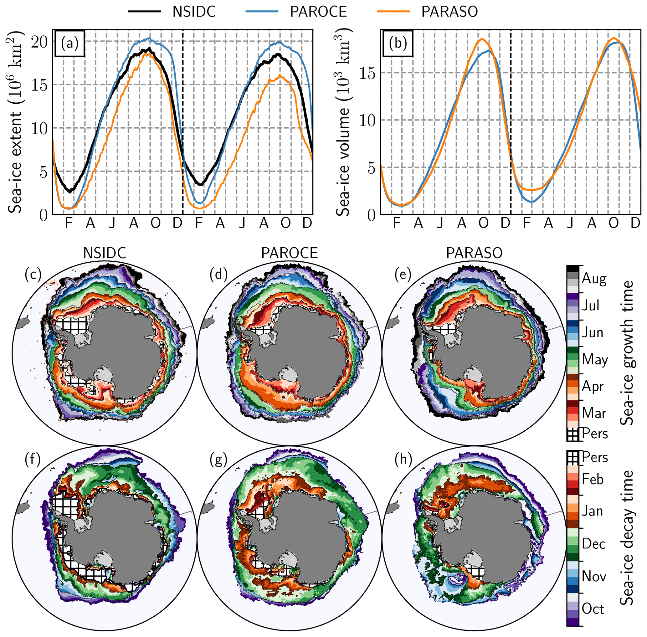
Figure 8 (a) Daily sea-ice extent from observations (NSIDC-G02315), PAROCE and PARASO, over 2000–2001. (b) Same for sea-ice volume (no observations available). (c–e) Sea-ice growth progression over the 2000 freezing season from (c) observations (NSIDC-0051), (d) PAROCE and (e) PARASO. The shadings indicate the earliest time of the year at which sea ice appears after the yearly minimum (in February 2000). (f–h) Same for the sea-ice decay progression over the 2000–2001 melting season. The shadings indicate the earliest time of the year at which sea ice disappears after the yearly maximum (early September 2000). On both color bars, “pers” indicates persisting sea ice throughout each full freezing or melting process. Sea-ice presence is defined by a 15 % concentration threshold.

Figure 8 displays sea-ice observations (sea-ice index from the National Snow & Ice Data Center, Fetterer et al., 2017) and diagnostics from PAROCE and PARASO. Generally speaking, the PARASO Antarctic sea-ice extent seasonal cycle shares similar features compared to PAROCE (see Fig. 8a), with larger biases. The chronology of the first-year cycle (i.e., dates of maximum and minimum) is well simulated, still with both configurations retaining too little sea ice in the summer (minimum extent at ≈10⁶ km² instead of 3×10⁶ km²), which is a persistent bias for most coupled models (Turner et al., 2013; Mahlstein et al., 2013; Roach et al., 2018, 2020). PAROCE and PARASO also suffer from another well-known bias in forced NEMO simulations, displaying too large maximal Antarctic sea-ice extent and too rapid subsequent melting (Vancoppenolle et al., 2009; Rousset et al., 2015; Barthélemy et al., 2018). The second-year PARASO seasonal cycle is considerably degraded compared with the first year, with a more significant low bias in maximum sea-ice extent (16 × 10⁶ km² instead of 18 × 10⁶ km²). In contrast with the sea-ice extent, the PARASO maximum sea-ice volume is generally larger than PAROCE's (see Fig. 8b). This may be linked to the relatively stronger PARASO winds and their coastward orientations, making sea ice more compact but less extensive (see Fig. A7). Regarding the sea-ice growth cycle (Fig. 8c–e), the PAROCE and PARASO biases are similar, with the PARASO growth being delayed by about 15 d compared to PAROCE, which then translates into smaller maximum sea-ice extent. On the other hand, in many regions, the PARASO sea-ice decay cycle (Fig. 8f–h) occurs much earlier than PAROCE. The clearest examples are the Indian and western Pacific sectors, whose decay cycles start from a too small cover, and where the formation of coastal polynyas linked to strong katabatic winds (see Fig. A7) contributes to leaving only a thin sea-ice strip from mid-December on. In western Antarctica, virtually no sea ice is present in PARASO from mid-December on, whereas in observations it can persist year-round (and in PAROCE, melt 1 month later). In the Ross and Bellingshausen seas, most of the sea-ice melt is occurring more than a month earlier in PARASO compared with PAROCE, which is in better agreement with observations. In comparison with the aforementioned regions, the PARASO sea-ice pack in the Weddell sector melts later, but still leaves smaller persisting sea-ice cover compared to PAROCE. The only exception to this rapid PARASO sea-ice decay lies in front of the Ross Ice Shelf, where strong winds blowing towards the coast lead to the formation of a large and thick persisting sea-ice pack (see Fig. A7).

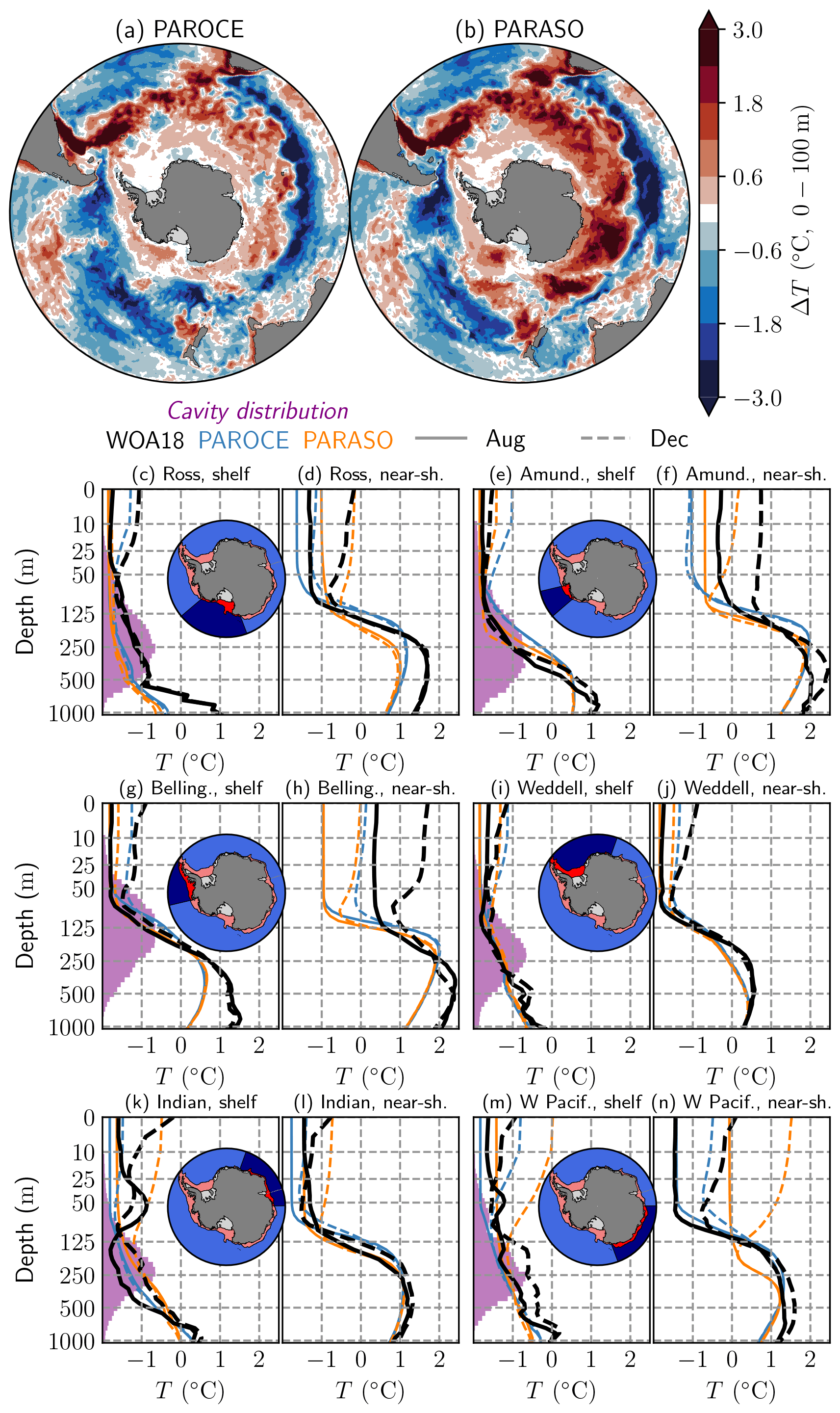
Figure 9 (a–b) In situ temperature biases for (a) PAROCE and (b) PARASO, with respect to the World Ocean Atlas 2018 (WOA18), averaged on the top 100 m of the ocean and the full seasonal cycle. (c–n) In situ temperature vertical profiles for WOA18, PAROCE and PARASO, in August (full) and December (dashed), over six circumpolar basins drawn on indicative maps. Note the nonlinear z axis. On the indicative maps, bright red shadings indicate the continental shelf (defined by the 1200 m isobath; see panels c, e, g, i, k, m); dark blue shadings indicate the “near-shelf” area (see panels d, f, h, j, l, n), defined as the area outside of the continental shelf and south of 60^∘ S. On the continental shelf vertical profile panels (c, e, g, i, k, m), the purple shadings represent each sector's vertical distribution of ice-shelf cavity presence (i.e., sector-specific, horizontally integrated area of ice-shelf-cavity–open-ocean interfaces, in normalized units). For WOA18, the data are taken from a 1995–2004 climatology; for PAROCE and PARASO, they are taken from simulation outputs for the year 2001 (second simulated year).

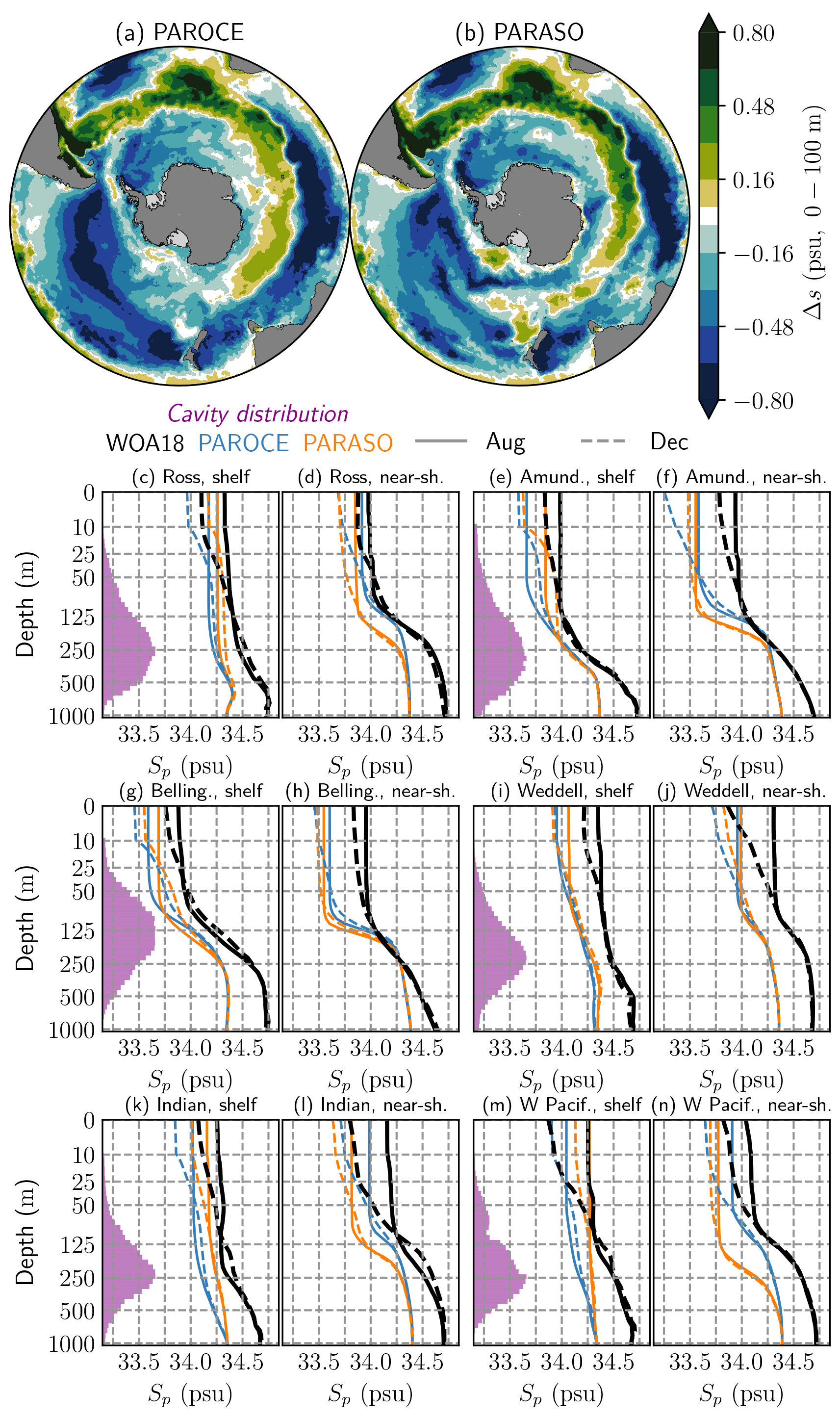
Figure 10 (a–b) Practical salinity biases for (a) PAROCE and (b) PARASO, with respect to WOA18, averaged on the top 100 m of the ocean and the full seasonal cycle. (c–n) Practical salinity vertical profiles for WOA18, PAROCE and PARASO, in August (full) and December (dashed), over six circumpolar basins (same as Fig. 9). Note the nonlinear z axis (following the NEMO vertical discretization). For WOA18, the data are taken from a 1995–2004 climatology; for PAROCE and PARASO, they are taken from simulation outputs for the year 2001 (second simulated year).

Figures 9 and 10 show in situ temperature and practical salinity diagnostics from the regridded World Ocean Atlas 2018 (Boyer et al., 2018), as well as those from PAROCE and PARASO. The PARASO temperature and salinity biases are generally similar to PAROCE's, even close to the air–sea interface (Figs. 9a–b and 10a–b). This can be explained by the NEMO initialization, which starts from a biased mean state corresponding to this specific configuration's equilibrium. It should however be noted that in PARASO, the eastern Antarctic subsurface is perceivably warmer and less saline than in PAROCE, matching the increased ice-shelf melt rates observed in Sect. 5.1. This is also related to the very rapid sea-ice decay in that area: from early spring, the ocean surface can undergo warming and the enhanced sea-ice melting leads to additional early freshwater release. An examination of the vertical profiles drawn in Figs. 9c–n and 10 confirms that the main origins of PARASO biases are related to the initialization, since they are similar to PAROCE. In general, deep waters are too cold ($\mathrm{\Delta }T\approx -\mathrm{1}$ ^∘C) and fresh (ΔP_s≈0.25 psu) in both PAROCE and PARASO. One possible cause for this bias is the presence of ice-shelf meltwater injection at depth, which is a novel feature for both configurations. While these general biases are present, the vertical structure of the water column is represented well within PARASO, and interseasonal changes are of the same magnitude as in WOA18.

In 2001, the Antarctic Circumpolar Current (ACC) transport through the Drake Passage is 47±4 Sv (1 Sv =10⁶ m³ s⁻¹) in PAROCE and 43±4 Sv in PARASO (see also Fig. A6). This is severely underestimated compared with observations (e.g., 173.3±10.7 Sv in Donohue et al., 2016) or other simulations (e.g., 117 Sv in Mathiot et al., 2011). The only directly identified cause of Drake ACC weakening in PARASO is the presence of spurious westwards currents along the Antarctic continental shelf (29 Sv) counterbalancing the eastwards transport, thus leading to a degraded net transport. While both PAROCE and PARASO Drake transport values display large biases, which will be a tuning focus for the NEMO configuration, the fact that the values are not significantly different from each other suggests that the coupling itself does not bear a significant impact on ACC transport.

5.3 Atmosphere

Figure 11 shows seasonally averaged 2 m air temperature differences between PARASO and ERA5. Large differences (up to 15 ^∘C in absolute value) are found over the ice shelves and the ocean close to Antarctica. The differences are much smaller in summer (Fig. 11a) compared to the winter season (Fig. 11c), when more sea ice is present and the atmosphere over the ice shelves is very stable. Over the Ross and Filchner–Ronne ice shelves, the 2 m air temperature is systematically lower in PARASO than in ERA5. This systematic difference is too large to be solely attributed to differences in elevation between PARASO and ERA5 over the ice shelves, but this effect might contribute to the temperature signal visible over the Berkner and Roosevelt islands. Due to the scarcity of in situ observations over the ice shelves, a fraction of the difference between PARASO and ERA5 may be due to uncertainties in ERA5 (Gossart et al., 2019). Moreover, differences of comparable magnitude, but of opposite sign, are observed when comparing PARASO with the Japanese 55-year Reanalysis (JRA-55; see Fig. A3). PARASO was also compared to AEROCLOUD, a pre-existing CCLM² stand-alone experiment that was thoroughly evaluated using in situ observational data (not shown; Souverijns et al., 2019). While it was found that both experiments behave similarly on the Filchner–Ronne Ice Shelf, the PARASO–AEROCLOUD differences over the Ross Ice Shelf were similar to the PARASO–ERA5 ones, hinting that the bias development in that sector is likely related to the coupling. The boundary layer over the ice shelves is very stable and the large differences between ERA5, JRA-55, PARASO and AEROCLOUD are probably related to deficiencies in the representation of turbulent fluxes in the boundary layer, which is known to be a considerable challenge in polar regions (e.g., Cerenzia et al., 2014; Vignon et al., 2018, and references therein). Due to the lack of data over the ice shelves, it is difficult to definitively attribute this deficiency to one of the products mentioned above.

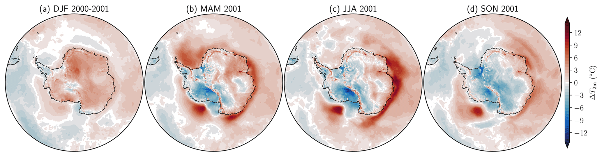
Figure 11 (PARASO–ERA5) differences in seasonally averaged 2 m air temperature for the second simulated year.

Over the ocean, the PARASO–ERA5 differences are largest in the East Antarctic sector, where the 2 m air temperature is systematically higher in PARASO than ERA5. This is consistent with the increased ice-shelf melt rates (see Sect. 5.1) and near-surface ocean warming (see Sect. 5.2) previously highlighted in this sector. In addition to ERA5 and AEROCLOUD, PARASO was also compared to PARATMO (see Table 4), a CCLM² stand-alone run with the same tuning parameters as for PARASO, except for the surface flux tiling which has not been implemented for CCLM² stand-alone experiments (instead, sea ice is assumed to fully cover a grid cell where the surface temperature is lower than −1.8 ^∘C). The large East Antarctic warm difference is less prevalent in PARATMO (see Fig. A4), thus suggesting an origin related to coupling. Moreover, in PARASO, large positive temperature anomalies are simulated over a restricted area in the Ross Sea. They are associated with the development of an open-ocean polynya, where the excessive vertical mixing induces the release of a substantial amount of energy. Some deep convection and open-ocean polynya formation have occurred during the past decades in the Southern Ocean, but many atmosphere–ocean–sea-ice coupled climate models that participated in the latest CMIP6 simulate them too frequently and at locations where they have not been observed (Heuzé, 2021), such as in the Ross Sea in PARASO.

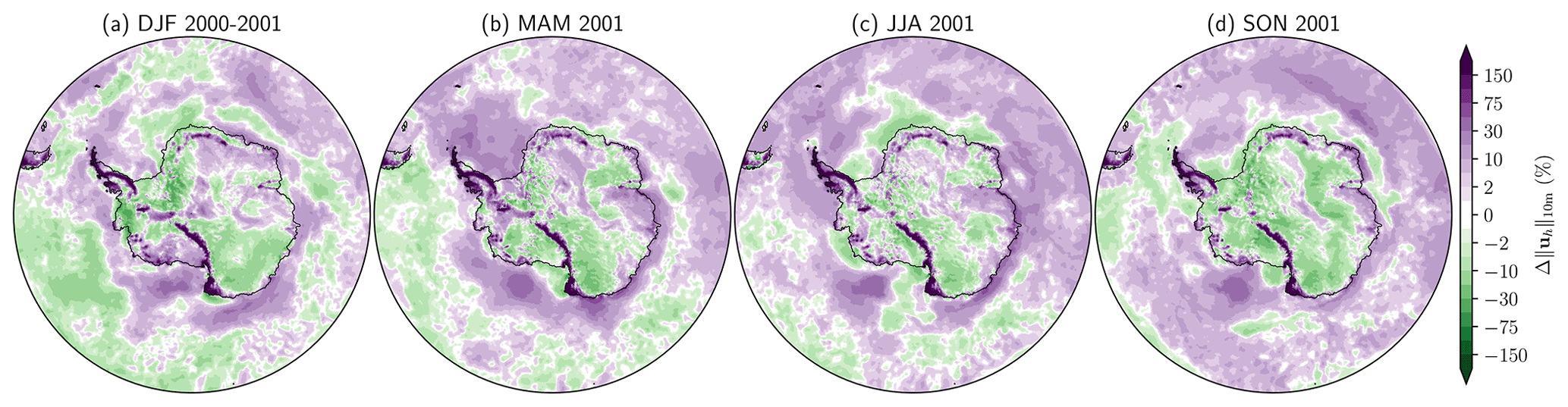
Figure 12 Relative differences in seasonally averaged 10 m horizontal wind speed norm between ERA5 and PARASO (i.e., (PARASO–ERA5)/ERA5). Note the nonlinear color scale.

Figure 12 displays the relative differences in seasonally averaged 10 m horizontal wind speed between PARASO and ERA5. Major differences are located in the Antarctic Peninsula and the Transantarctic Mountains. There, the magnitude of the PARASO winds can be more than twice the value in ERA5, with little interseasonal differences. More generally, the regions of highest wind speed differences match the regions where the elevation differs the most. The effect of subgrid-scale orography is accounted for through an effective roughness length (Lott and Miller, 1997), which is likely lower in PARASO compared to ERA5. Over the continent, outside of mountainous regions, the surface wind speed is generally lower in PARASO than ERA5. Gossart et al. (2019) showed that ERA5 underestimates the 10 m wind speed in coastal areas and the interior of Antarctica. Similar conclusions apply to PARASO.

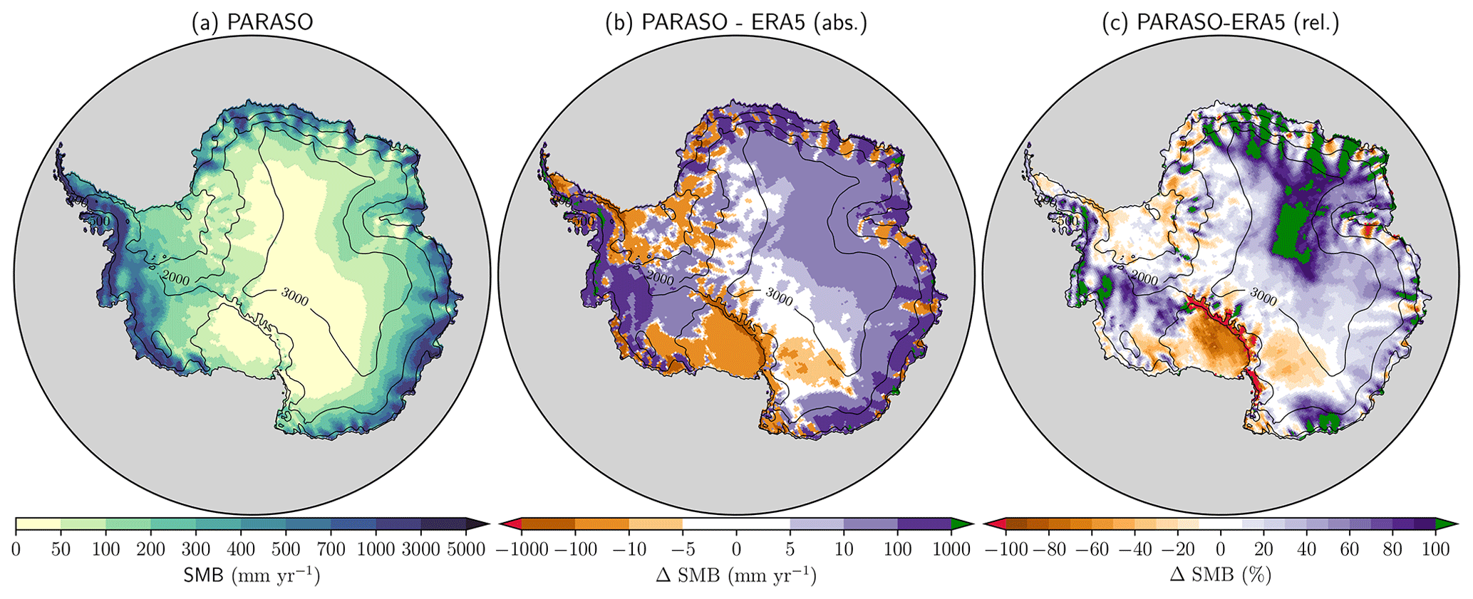
Figure 13 Surface mass balance reconstruction for 2001, the second simulated year. (a) PARASO; (b) PARASO absolute difference w.r.t. ERA5; (c) PARASO relative difference w.r.t. ERA5. Note the nonlinear color scales. Contours denote elevation at 500, 2000 and 3000 m above mean sea level.

The differences in PARASO and ERA5 SMB, calculated as total precipitation minus surface sublimation, are displayed on Fig. 13. Precipitation is the dominant source of the Antarctic ice-sheet SMB. Accordingly, the differences in SMB between PARASO and ERA5 primarily result from differences in the simulated precipitation. As surface melt runoff (only significant for areas below 1000 m elevation) is not included and snowdrift processes are not represented, the estimated SMB may depart from observations. However, the scarcity of in situ observations prevents us from accurately estimating the AIS SMB, and we chose to compare our SMB estimate to ERA5, whose quality is discussed in Gossart et al. (2019). Moreover, in Mottram et al. (2021), SMB estimates from different Antarctic regional climate models (including CCLM²) are compared, and the observed intermodel spread suggests considerable uncertainties even in uncoupled, atmosphere-only simulations.

Compared to ERA5, PARASO provides higher SMB values over East Antarctica and the Weddell Peninsula (Fig. 13). For East Antarctica, the largest differences are located in the coastal areas, where the SMB in PARASO can be more than twice the SMB in ERA5. Those differences may partly result from a too low SMB estimate in ERA5, particularly below 500 m elevation (Gossart et al., 2019). Souverijns et al. (2019) found, when investigating the spatial pattern of the simulated SMB in AEROCLOUD with the reconstruction based on ice cores and ERA-Interim of Medley and Thomas (2018), a significant underestimation of the SMB for most of the coastal sites including the Antarctic Peninsula. A comparison of PARASO to AEROCLOUD reveals higher SMB values in those regions, suggesting a better agreement with observations. Irrespective of the comparison product used (AEROCLOUD or ERA5), PARASO simulates lower SMB values over the Ross Ice Shelf. This is primarily attributed to less precipitation in PARASO over this region (not shown). We also analyzed the SMB provided by PARATMO (see Fig. A5), for which similar results to PARASO are found. This argues that the model behavior can at least be partly related to the representation of atmospheric dynamics and not solely to the coupling.

6 Discussion and conclusions

In this technical paper, we have introduced PARASO, a new five-component coupled configuration for simulating the Earth system in the high latitudes of the Southern Hemisphere. Aside from the novel coupling interfaces, establishing this new tool required substantial model developments in the COSMO atmosphere model, in order to adapt its surface scheme to requirements from NEMO (mostly related to flux tiling), the ocean–sea-ice model it is coupled to in PARASO. To our knowledge, PARASO is the first publicized circumpolar Antarctic ocean–atmosphere coupled regional configuration that includes an ice-sheet model, with ice-shelf cavities explicitly resolved. The ocean–ice-sheet offline coupling interface has also been thoroughly described in this paper. However, our results suggest that at the short timescales investigated for this technical paper, the practical impact of this particular coupling interface is minor, and that the main features of PARASO would be reproduced with a similar NEMO–CCLM² coupled configuration (i.e., excluding coupling with f.ETISh). As briefly mentioned in Sect. 5.1, even at longer timescales (40 years), the ice-sheet initialization appears to be more determining than the presence of an ocean–ice-sheet coupling interface.

In addition to the functioning of the coupling interfaces, the major PARASO achievement lies in its numerical stability. Yet, the specific biases observed in PARASO (e.g., warm and moist near-surface bias in eastern Antarctica, generalized excessive latent heat over sea ice, the representation of stable atmospheric boundary layers above ice shelves) are a significant drawback, which prevents PARASO from being considerably more skillful than some global coupled configurations. Global climate models suffer from similar biases in the high latitudes of the Southern Hemisphere (Wang et al., 2014; Schneider and Reusch, 2016) and the PARASO biases are of comparable magnitude to the differences between distinct reanalyses (see Figs. 11 and A3).

Overall, PARASO is a novel tool and further calibration could reduce the biases. For this first evaluation of our tool, the objective was to check whether the biases were affected by the coupling interfaces themselves (which they are not), rather than to correct the more general issue related to each model's biases. Extra tuning for limiting biases introduced by our choice of model combination and data input changes is however of high priority. While recognizing that clearly distinguishing each PARASO component's contribution to the biases from those purely due to their coupling interfaces is far from straightforward, we consider the former to be beyond the scope of this study.

Besides the coupling itself, the PARASO biases may be imputable to changes in each model's configuration that led to apply each component in conditions different from the ones in which they were developed and calibrated. Yet, our choice has been to retain these changes, since they are relevant. For example, taking the Antarctic surface topography from f.ETISh as initial CCLM² geometry instead of the standard dataset made the PARASO setup more consistent intermodel-wise. However, CCLM² parameters had been tuned to this standard topographical dataset, and this might have impacted the results. In other words, we have preferred fundamental consistency over the precise agreement with current observations. Incorporating our novelties while limiting biases also identifies clear paths for model improvements. Below, we provide three potential bias sources and perspectives related to their corrections or limitations. We also refer to Appendix E for more details on tuning experiments which have led to PARASO, as the “out-of-the-box” coupling between PARASO components led to even stronger biases.

First, in the vicinity of their common interface, the ocean and atmosphere are highly sensitive to their boundary conditions (Miller et al., 1992; Large et al., 1997; Torres et al., 2019a, b). For PARASO, the interface boundary condition has been altered on both sides for enforcing COSMO–NEMO intermodel compatibility. Besides being assessed from a dynamical model instead of an external dataset (such as a reanalysis), ocean–atmosphere fluxes are computed differently in PARASO compared to either NEMO or COSMO stand-alone experiments. On the NEMO side, the ocean receives turbulent fluxes from the COSMO surface scheme instead of an ocean-calibrated bulk formula (e.g., CORE Large and Yeager, 2004). Performing NEMO stand-alone experiments with a COSMO-derived bulk formulation is a considerable challenge, as the COSMO surface scheme requires several near-surface atmosphere properties (e.g., TKE at bottom levels or laminar transfer coefficients) as input. On the COSMO side, the atmosphere receives tiled fluxes which harbor subgrid-scale heterogeneity in surface properties. Since the COSMO surface scheme has been tuned for non-tiled fluxes (it uses instead a binary approach), the new tiling method, which is a requirement for coupling with NEMO, may lead to undesired systematic biases. Performing COSMO stand-alone experiments with tiled fluxes has not been pursued because this would have required further adapting the COSMO sources and forcing datasets. In a recent study, Heinemann et al. (2021) present a nonlinear tiling approach for COSMO (similar to that of PARASO) as an enhancement of a non-conserving method (Gutjahr et al., 2016), which also relies on sea-ice thickness (not considered in PARASO). This may be of use for future studies intending at investigating the sole impact of non-binary tiling. Alternative approaches are possible to locally reduce the biases in the air–sea fluxes, in particular by nudging them to reanalysis data, as done for instance in Ho-Hagemann et al. (2020) in a recent study coupling NEMO and COSMO. This has the advantage of providing model results closer to observations but at the cost of perturbing the atmosphere–ocean feedbacks and adding artificial energy sources and sinks at the surface, thus limiting the applications of the model outside of present-day conditions.

Second, coupled PARASO experiments suffer from excessive latent heat (and thus evaporation) over sea ice, as illustrated in Fig. E1e. Since coupled and forced snowfall rates are roughly similar (not shown), this evaporation bias is the main driver beneath the observed decrease in snow thickness over sea ice (see Fig. E1c). This leads to a positive feedback further inhibiting the presence of snow over sea ice and thus the radiative balance at the sea-ice surface: the excess of evaporation degrades the snow cover, the surface albedo is reduced, more solar radiation is absorbed by the sea-ice–snow system; hence, even more snow melts at the surface. While some specific tuning (see Appendix E) helped reducing this bias, its positive feedback has not been fully controlled, and this aspect represents one of the main challenges for future PARASO developments.

Third, another potentially large source of biases is the updated Antarctic continent geometry used in PARASO. As described in Sect. 4.3, the initial Antarctic topography is derived from a f.ETISh relaxation run, which displays clear differences from observations, related to this model's specific biases and to the forcing datasets it relied on (SMB from COSMO, ice-shelf melt rates from NEMO). Out of inter-model consistency, all PARASO initial geometries have been directly derived from this f.ETISh relaxation run. In the atmosphere, the signature of the new topography can be seen on the differences between AEROCLOUD and PARASO (see Fig. 5 and Sect. 5.3). In the ocean, the near-Antarctic bathymetry is crucial to the warm water intrusion into the cavities, and thus to the ice-shelf melt rates (see Goldberg et al., 2019 for an overview). Results from 30-year NEMO–f.ETISh coupled experiments (without CCLM²; see Fig. A9) have suggested that at least on these timescales, the initial cavity geometry plays a much bigger role on ice-shelf melt rates than the ice-sheet–ocean coupling. This is to be expected, since the melt rates induced by the coupling on decadal timescales – and therefore the simulated cavity changes – are smaller than the ice geometry changes during the multi-millennial f.ETISh initialization (see Sect. 4.3).

The three sources of biases listed above have been mostly identified from comparison with the different stand-alone versions of each used model. However, other bias sources enhanced by the coupled nature of PARASO may also be present within this tool. As previously mentioned, the objective of this paper is to document our tool, assess its performance as is and share it with the community. Taking advantage of the numerical stability of PARASO and the expertise gained in its development process, additional tuning and calibration experiments aiming for further bias reduction are currently at the designing stage. Finally, it may be worth noting that in comparison with the short experiments of Sect. 5, the sea-ice extent biases remain stable or are even reduced with time in a longer fully coupled PARASO experiment (see Fig. A10). This suggests that the ocean surface warming described in Sect. 5 remains circumscribed to relatively small amplitudes; hence, PARASO does not keep on drifting in the longer term, and its performance remains reasonably satisfactory at least in terms of Antarctic sea ice.

Appendix A: Additional figures and tables

(ice strength; see Hibler, 1979)

Table A1 List of key NEMO parameters (excluding those related to ice-shelf cavities, which are already covered in Table 1).

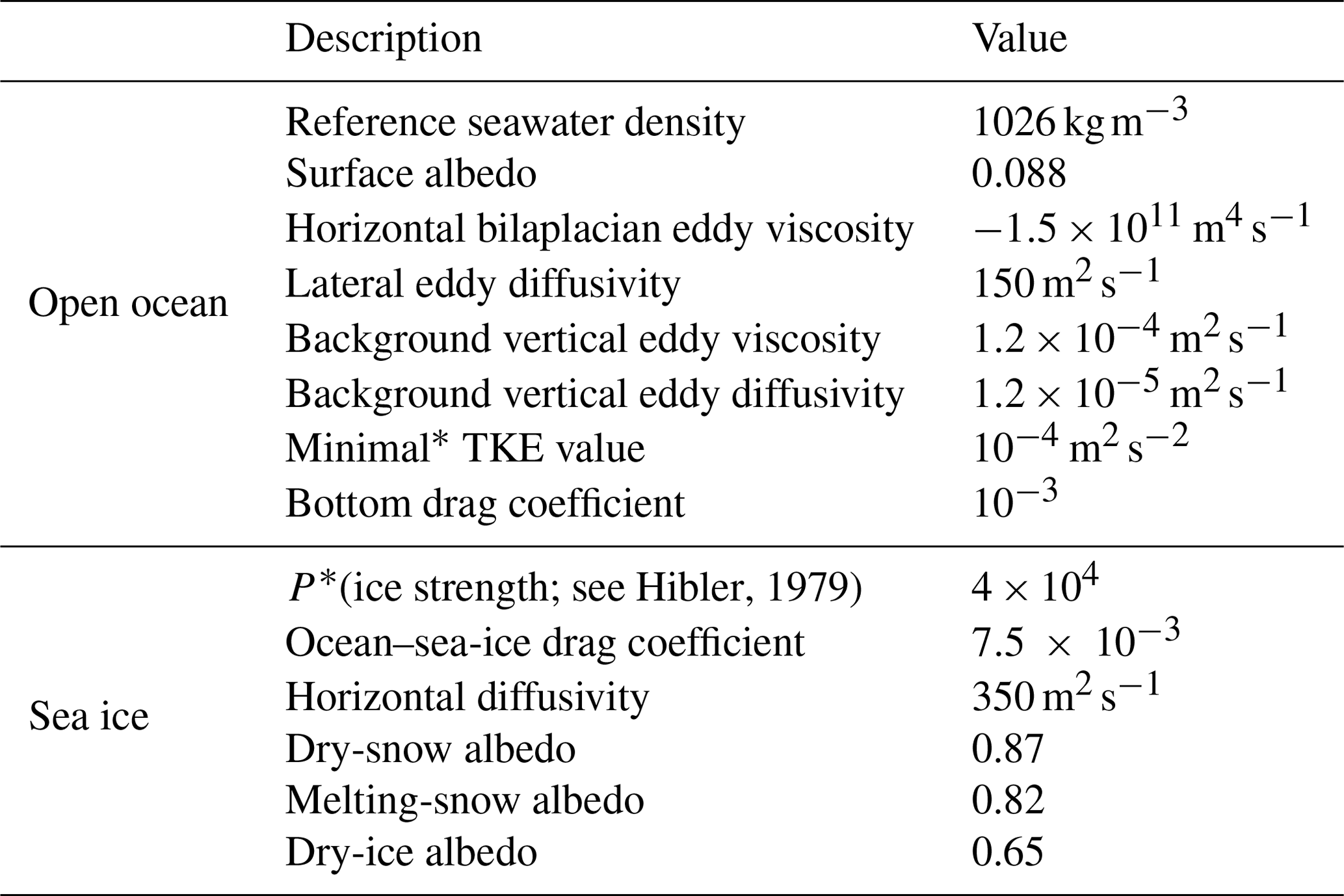
^* The TKE is brought back to this threshold in the event that computations lead to lower values.

Mellor and Yamada (1982)(Doms et al., 2018)Doms et al. (2018)Ritter and Geleyn (1992)(Liston et al., 2007)(Vionnet et al., 2012)(van Kampenhout et al., 2017)

Table A2 List of key CCLM² parameterizations.

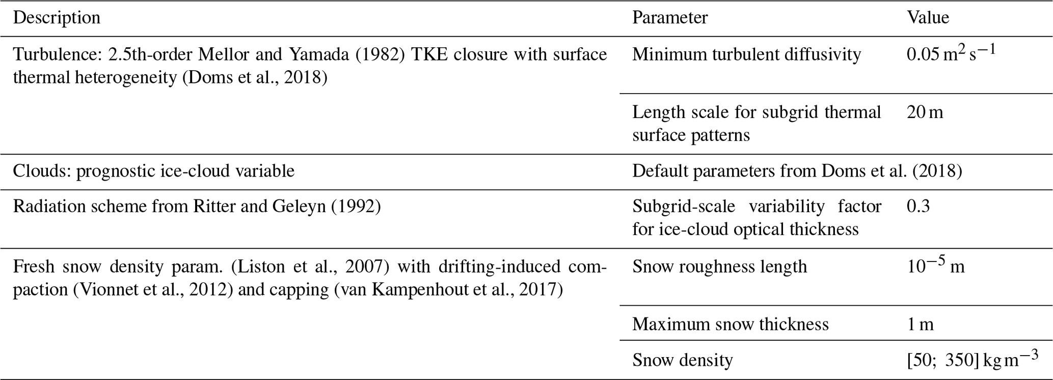
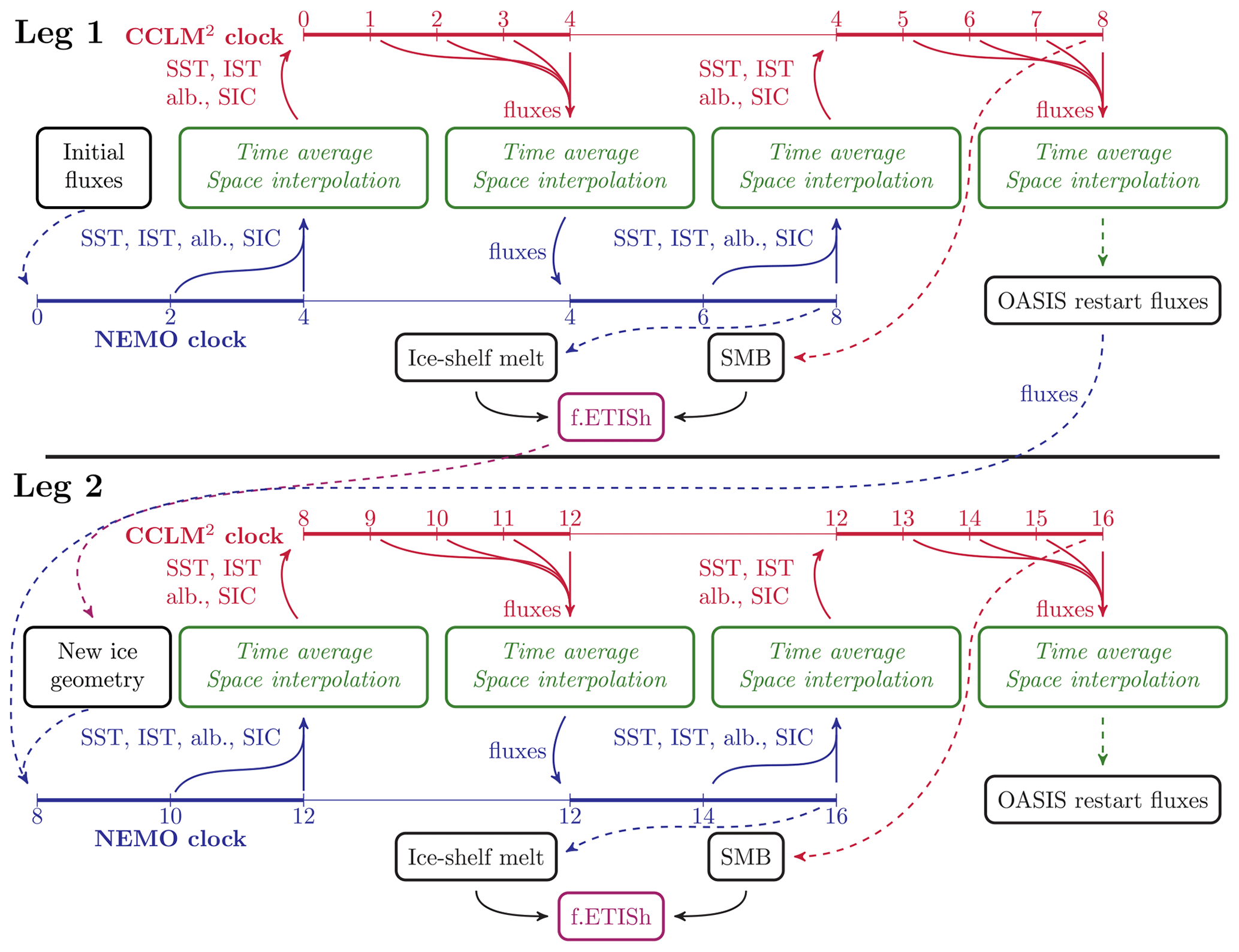
Figure A1 Fully coupled system timing scheme. Here, two restart legs are represented, separated by the thick horizontal line. The top and bottom timelines represent the NEMO and CCLM physical clocks, respectively. They are deliberately staggered to account for NEMO receiving delayed fluxes. For the sake of readability, above the CCLM, the time step is 1, NEMO's is 2, the NEMO–CCLM coupling frequency is 4 and the ice-sheet model coupling frequency is 8. In between legs, the NEMO–CCLM system is stopped. Black boxes represent data written on the disk. Green boxes represent OASIS operations. Full arrows represent exchange of data between models and OASIS. Dashed lines represent reading or writing to disk. “SST” stands for sea surface temperature; “IST”, ice surface temperature; “alb.”, albedo; “SIC”, sea-ice concentration; “SMB”, surface mass balance.

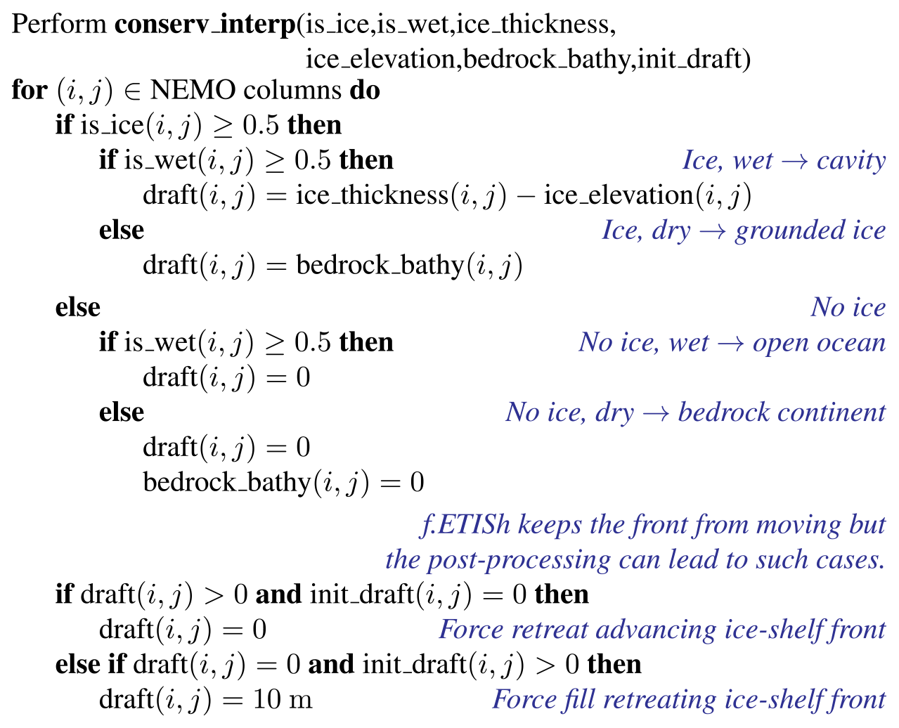
Figure A2 Pseudocode for the ice-sheet geometry post-processing. “conserv_interp” is a conservative interpolation from f.ETISh's grid to NEMO's. On the f.ETISH grid, “is_ice” is 0 for the open-ocean column, else (cavity or grounded ice) it is 1; “is_wet” is 0 for grounded ice, else (cavity or ocean) it is 1. “draft” is the ice-shelf draft; like the bedrock bathymetry, it is positive downwards and set to zero at the ocean surface. “ice_elevation” is the ice surface elevation compared to floating point level, defined positive upwards. “init_draft”, the initial NEMO ice-shelf draft, is used to ensure that the procedure has not led to ice-shelf front displacement.

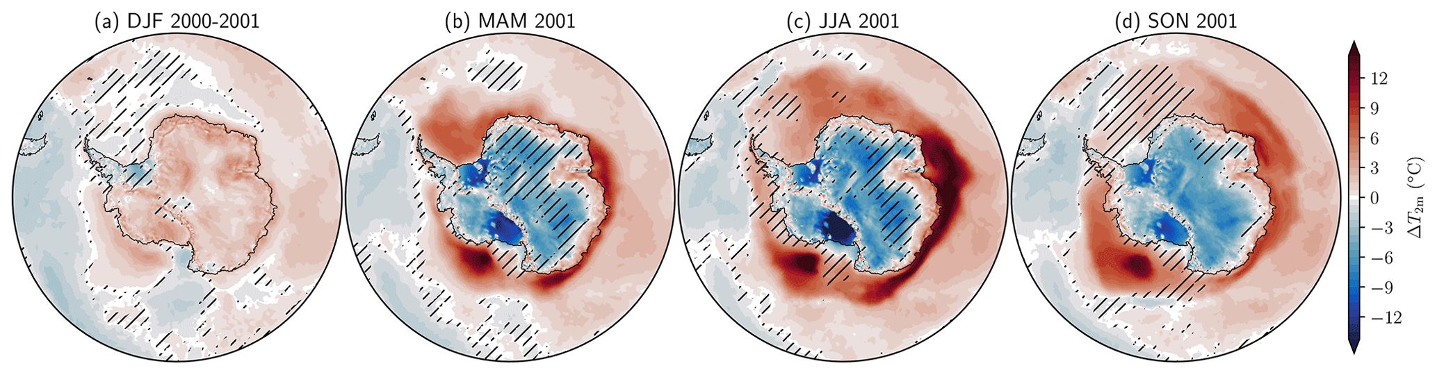
Figure A3 (PARASO–JRA-55) (Kobayashi et al., 2015) differences in seasonally averaged 2 m air temperature for the second simulated year. The used color bar is the same as that in Fig. 11. Hatching denotes areas where the PARASO–JRA-55 and PARASO–ERA5 (see Fig. 11) differences are of contrary signs.

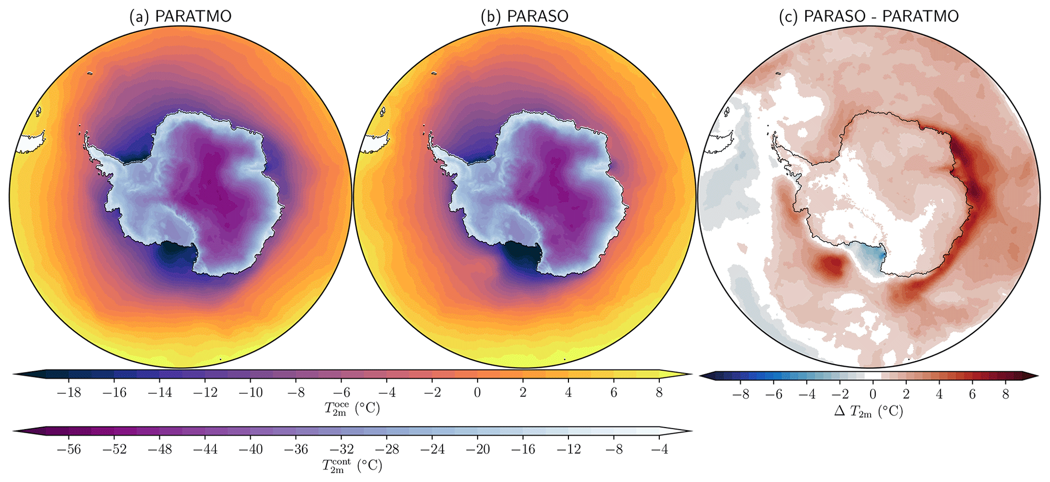
Figure A4 The 2001 average of 2 m air temperature for (a) PARATMO, (b) PARASO and (c) the PARASO–PARATMO difference. Note that in panels (a)–(b), distinct color scales are used for the ocean (“oce”) and continent (“cont”).

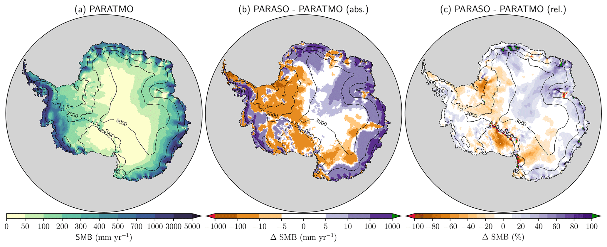
Figure A5 2001 average of SMB for (a) PARATMO, (b) PARASO–PARATMO absolute difference and (c) PARASO–PARATMO relative difference. Note the nonlinear color scales. Contours denote elevation at 500, 2000 and 3000 m above mean sea level.

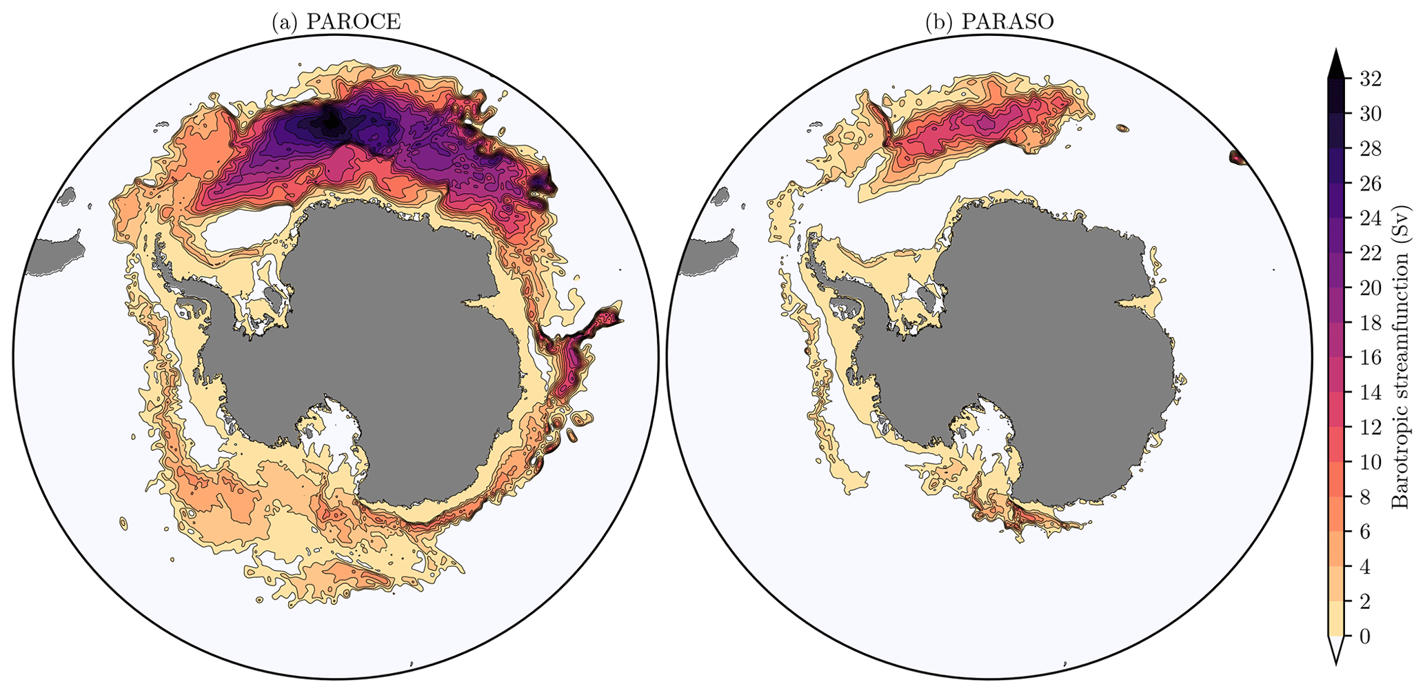
Figure A6 Barotropic streamfunction for (a) PAROCE and (b) PARASO, averaged over 2001 (second simulated year), in Sv (1 Sv = 10⁶ m³ s⁻¹). The streamfunction has been set to zero over Antarctica. Positive values indicate clockwise circulation. Negative values are not represented.

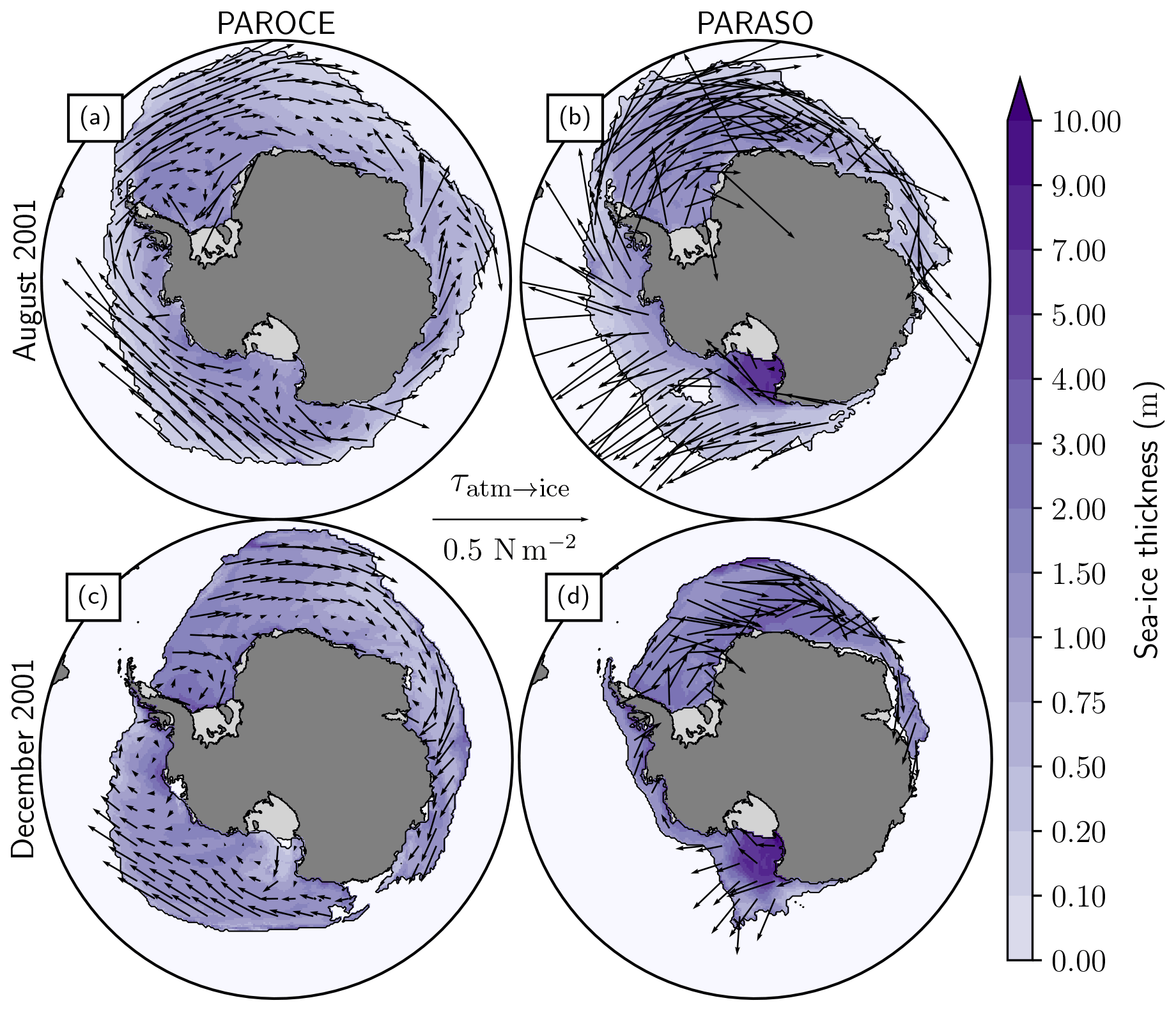
Figure A7 Sea-ice thickness (color map) and air–sea-ice wind stress (arrows) in (a, b) August and (c, d) December of 2001 (second simulated year), for (a, c) PAROCE and (b, d) PARASO. Sea-ice thicknesses are only drawn on areas with sea-ice concentrations exceeding 15 %. While the wind stress scale is linear, note that the sea-ice thickness scale is not.

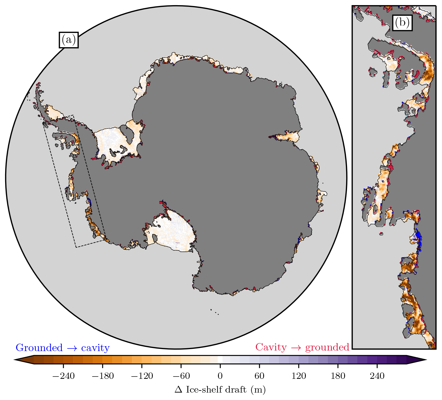
Figure A8 Differences between PARASO initial draft geometry taken from the f.ETISh initialization run (see Sect. 4.3) and BedMachine (Morlighem et al., 2020) (PARASO–BedMachine) for (a) the full Antarctic and (b) a western Antarctica zoom-in. Blue nodes indicate grounded columns in the BedMachine dataset that become cavities in the PARASO initial geometry. Red nodes indicate the opposite (cavity columns turning into grounded ones).

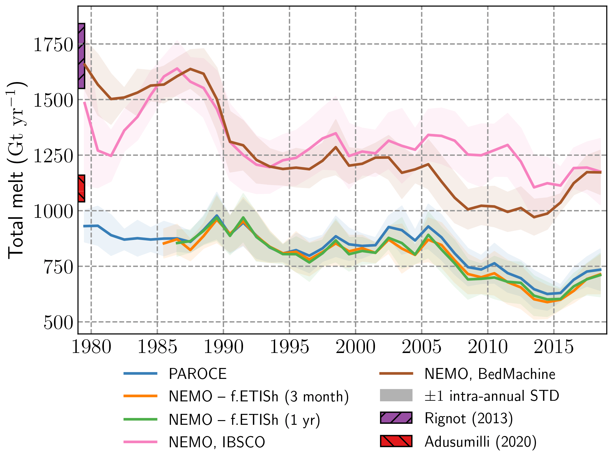
Figure A9 Integrated global Antarctic subshelf melt rates from different experiments (lines) and observational estimates (bars). “PAROCE” is presented in Sect. 5.2. The two “NEMO–f.ETISh” experiments share the same initial bathymetry derived from the initialization described in Sect. 4.3, and feature ocean–ice-sheet coupling (no CCLM²) at distinct frequencies (3 months and 1 year). “NEMO, IBSCO” and “NEMO, BedMachine” are obtained from NEMO stand-alone experiments, with bathymetry and static cavity geometry taken from the International Bathymetric Chart of the Southern Ocean (Arndt et al., 2013) and BedMachine v2 (Morlighem et al., 2020), respectively. Observational datasets are taken from Rignot et al. (2013) and the steady state of Adusumilli et al. (2020).

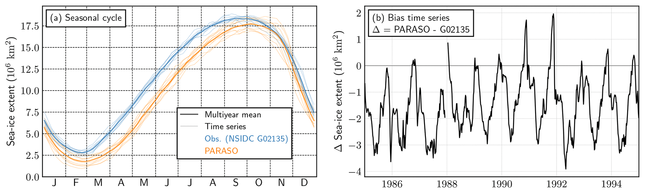
Figure A10 Antarctic sea-ice extent from observations (NSIDC-G02135, Fetterer et al., 2017) and from an additional fully coupled PARASO experiment (not presented here) covering the 1985–1994 period: (a) seasonal cycle and (b) bias time series (PARASO–NSIDC-G02135). In panel (b), the gap around 1988 is due to a shortage in observational data.

Appendix B: Computational aspects

B1 Numerical stability

While only one 2-year simulation is presented in this paper, a considerable amount of sensitivity and tuning experiments have been performed for this study. In total, over 50 years of equivalent fully simulated years have been performed with the final PARASO source code, mostly for limiting the large bias developments. With these “latest” sources (distributed throughout this paper), no numerical instability has been observed yet, which suggests that PARASO can be considered as numerically stable. In our case, this was achieved by

• reducing the COSMO time step from its AEROCLOUD (Souverijns et al., 2019) value of 120 s to 90 s, in order to avoid CFL-criterion errors – such errors may probably be linked to the finer PARASO vertical resolution compared with AEROCLOUD (+50 %); and

• adapting the land “transfer coefficient limiter” implemented in COSMO by Davin et al. (2011). Over land, CLM computes all fluxes (including turbulent ones) and sends them to COSMO. However, the COSMO vertical physics scheme requires transfer coefficients (C_D, C_H) and surface properties (T_S, q_s) instead of fluxes per se. Hence, transferred coefficients are re-evaluated from CLM-originating fluxes through dividing by the near-surface temperature and moisture gradients (for sensible and latent heat, respectively). In cases where the surface temperatures (moisture) are very close to near-surface ones, this may lead to floating-point instabilities (small flux divided by small gradient), which can generate very large heat fluxes and subsequent crashes. In some of our tuning simulations, such crashes have been formally identified and traced from time-step-by-time-step COSMO outputs. Hence, in our simulation, $\left|C_{\mathrm{H}}\right|$ is limited to 10⁻².

B2 Performance and load balancing

The PARASO experiments presented here have been performed on the Skylake nodes of the Flemish Tier-1 Breniac cluster. We asked for 224 cores running at 2.6 GHz. With these resources, the wall time was about 3.5 h for 1 month of simulated time. This includes all models and their I/O, as well as the offline f.ETISh coupling interfaces. Figure B1 displays the wall time required for simulating 1 month and the parallel efficiency of PARASO, defined as

$$\begin{array}{}\text{(B1)}& e\left(n_{\mathrm{proc}}\right)={\displaystyle \frac{n_{\mathrm{proc}}^{\min }T\left(n_{\mathrm{proc}}^{\min }\right)}{n_{\mathrm{proc}}T\left(n_{\mathrm{proc}}\right)}},\end{array}$$

where n_proc is the number of cores used; $n_{\mathrm{proc}}^{\min }=\mathrm{56}$ is the minimal number of cores required for PARASO (constrained by random access memory requirements); and T(n_proc) is the wall time required for 1 month of PARASO simulated time. As Fig. B1 shows, PARASO scales reasonably well up to  ≈10³ cores.

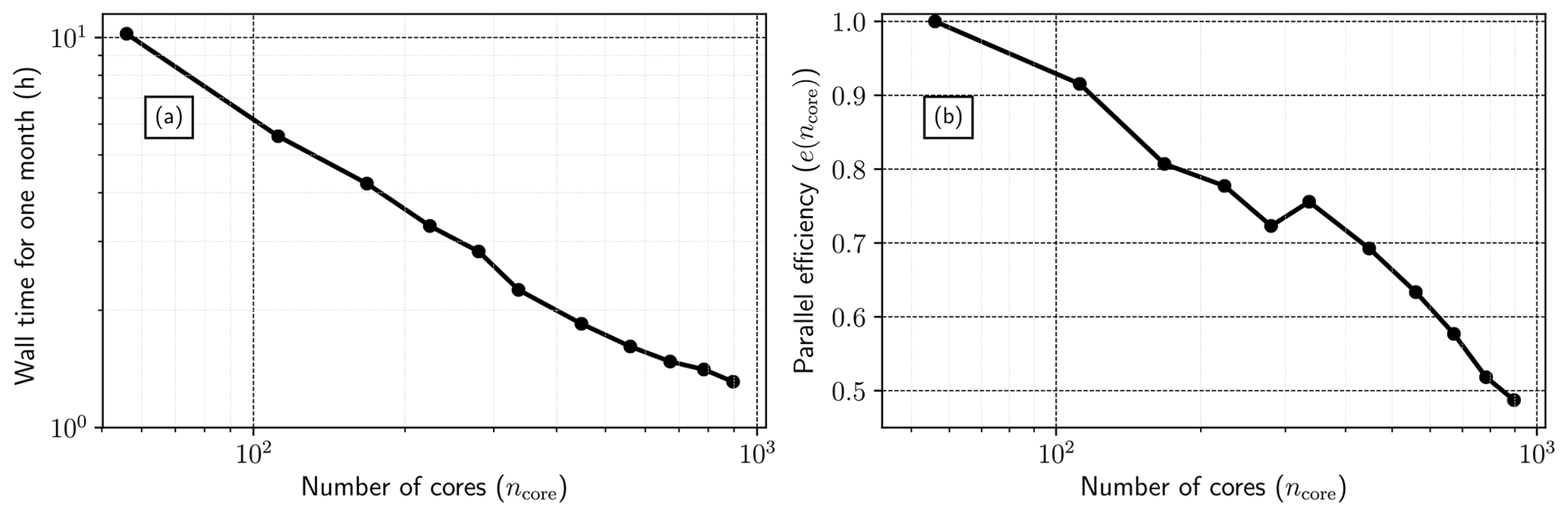
Figure B1 (a) Wall time required for simulating 1 month and (b) parallel efficiency of PARASO (see Eq. B1). Note that in panel (a), both axes are log scaled; in panel (b), the x axis is.

Table B1 Intermodel load balancing. XIOS is the NEMO I/O program, which is run as a separate executable. f.ETISh is not listed here, as it is run in between NEMO–CCLM² legs.

Message Passing Interface (MPI)-based domain decomposition parallelism is implemented in NEMO, COSMO and CLM. The CPU balancing between these models, which is shown in Table B1, has been empirically tuned. As expected, COSMO is the biggest CPU consumer, amounting for about twice as much as NEMO or CLM, which use roughly equivalent resources. f.ETISh is not shown in Table B1, since it is run sequentially in between NEMO–CCLM² legs. Its computational cost is negligible (less than 0.1 %) compared with all other models listed in Table B1. The same applies for the f.ETISh-including offline coupling interfaces: the equivalent wall time they require is negligible compared to what is shown in Table B1. This was to be expected, as these coupling interfaces only process 2-D fields at relatively low temporal frequencies (monthly at most frequent).

B3 Replicability and restartability

Replicability and restartability are highly desirable properties for scientific models, but achieving them remains a considerable computer science challenge in the context of climate models (Massonnet et al., 2020). Like most climate model configurations, PARASO features restart procedures, during which the content of each model's prognostic variables is written to disk in order to interrupt the execution and limit the wall-time requirements. In PARASO, the restart procedure is also needed for the f.ETISh coupling, which is performed offline in between restarts. In other words, even with unlimited CPU time, PARASO would require restarts.

Restart procedures have been implemented in all used models, plus OASIS, which writes the content of the coupler at the end of a leg to ensure smooth restartability. Hence, PARASO restarts should theoretically be fully transparent (i.e., not have an impact on model trajectory), but empirically, it has been observed that this was not the case. Further experiments have identified COSMO as a potential source for non-restartability. Floating-point rounding errors (from double to single precision) employed in restart I/O may lead to potentially diverging trajectories (Corden and Kreitzer, 2015). The magnitude of the differences in NEMO trajectories induced by a restart is insignificant in comparison with that induced by a COSMO restart. This was to be expected, since the atmosphere is physically much more chaotic than the ocean.

While the PARASO experiment presented above has been performed on Breniac (Tier-1 cluster from the Vlaams Supercomputer Centre), the fully coupled setup has also been successfully run on Lemaitre3 (Tier-2 cluster from the French-speaking Belgian Consortium des Équipements de Calcul Intensif), without numerical instabilities. The non-transparency of restart procedures on one of them (Breniac) is a strong argument supporting the non-replicability across distinct architectures. It should however be noted that, roughly speaking, simulation results from both machines were similar to each other. Moreover, outputs from identically launched experiments on one given machine–architecture combination are identical, down to bit precision.

Appendix C: CCLM² differences between AEROCLOUD and PARASO

In this appendix, we list the major differences in the CCLM² model (tuning parameters, domain, parameterizations) between AEROCLOUD (a previous CCLM² stand-alone Antarctic configuration; see Souverijns et al., 2019) and PARASO.

The number of vertical levels in PARASO has been increased from 40 to 60. It allows a better representation of the stable boundary layer over the Antarctic ice sheet (Genthon et al., 2013; Handorf et al., 1999; King et al., 2006). The lowest full model level is located at 5 m (10 m) in PARASO (AEROCLOUD) and 14 PARASO levels (11 in AEROCLOUD) are located on the bottom 1000 m of the atmosphere. To prevent numerical instabilities related to this new vertical resolution from arising, the COSMO time step has been decreased from 120 to 90 s.

The spatial domain in AEROCLOUD is limited to the Antarctic ice sheet. To study the Antarctic climate variability at the decadal timescale, the PARASO domain has been extended to the whole Southern Ocean to explicitly simulate the interactions between the atmosphere and the ocean. The boundaries of the PARASO domain are thus located between 50 and 40^∘ S. The horizontal resolution is unchanged (0.22^∘).

In order to improve the representation of perennial snow and land surface processes, some Antarctic-specific adjustments have been made in AEROCLOUD. These adjustments concern

1. the representation of the snowpack in the Community Land Model following van Kampenhout et al. (2017);

2. the roughness length of snow to have a correct representation of the katabatic winds at the coastal margins of the Antarctic ice sheet and the ice shelves;

3. the turbulence scheme to account for the strong stable conditions.

More information can be found in Souverijns et al. (2019). The inclusion of the AEROCLOUD two-moment cloud-microphysics scheme is disregarded in PARASO, because over this extended domain and with the increased number of vertical levels, only small improvements were found in the representation of clouds and solid precipitation. The computational resources necessary are much larger than those needed for the default parameterization scheme based on the one-moment Kessler scheme used to calculate the effects of grid-scale clouds and precipitation.

Compared to AEROCLOUD, the spectral nudging has been switched off. A prime objective of future work with PARASO is to study the mesoscale interactions and their potential impact on larger-scale atmospheric and oceanographic structures. Accordingly, we did not impose any relaxation in the inner domain of the atmospheric model towards the large-scale driving model (ERA5). In this way, the CCLM² dynamics is preserved.

PARASO uses the default snow roughness length of CLM4.5 of $\mathrm{2.4}\times {\mathrm{10}}^{-\mathrm{3}}$ m, which is constant in time and space. This contrasts with AEROCLOUD, for which the snow roughness length had been set to 10⁻⁵ m. Moreover, PARASO uses the standard snow and ice module of CLM4.5 (Oleson et al., 2013) and does not include the modified scheme implemented in AEROCLOUD. Future sensitivity studies of the modified snow and ice scheme and of the value for the surface roughness length are planned.

In COSMO, the turbulence scheme uses a 1-D closure with a prognostic equation for TKE. To better represent very stable conditions over the Antarctic ice sheet, a reduction of the limit on the vertical diffusion coefficients has been considered in both AEROCLOUD and PARASO, based on Cerenzia et al. (2014). Practically, the minimal diffusion coefficients for vertical scalar (heat) transport is set to 0.05 m² s⁻¹ and the effective length scale of subscale surface patterns over land (used to compute the energy transfer from subgrid-scale coherent eddies to turbulent scale, and referred to as “thermal circulation term” in Cerenzia et al., 2014) is set to 20 m. Note that the values provided in Souverijns et al. (2019) for those two variables are incorrect, and that in the AEROCLOUD model integrations the values mentioned above were used.

Appendix D: CCLM tiling

Here, we describe the pseudo-averaging of ocean CCLM surface properties in order to conserve local energy in the subgrid-scale tiling. The pseudo-averaging operation has an impact on the CCLM-perceived surface temperature, surface moisture, turbulent transfer coefficients, laminar transfer coefficients, lowest-level TKE, lowest-level heat and momentum diffusivity, albedo and radiative surface temperature.

Throughout this appendix, the index $j=\mathrm{0},\mathrm{1}$ distinguishes both tiles, with j=0 corresponding to the open ocean and j=1 to the sea ice. $(f_{\mathrm{0}},f_{\mathrm{1}})\in {\left[\mathrm{0};\mathrm{1}\right]}^{\mathrm{2}}$ are the tile concentrations and satisfy $f_{\mathrm{0}}+f_{\mathrm{1}}=\mathrm{1}$.

The main novelties are linked to the TKE-derived surface transfer scheme (Doms et al., 2018). On every cell, this scheme updates

• κ, the TKE on the lowest level (defined on cell vertices), also used as input;

• 𝒦_m and 𝒦_h, the momentum and heat diffusivities, on the lowest level (defined on cell centers), also used as input;

• C_D and C_H, the turbulent momentum and heat transfer coefficients (in CCLM, the moisture transfer coefficient is C_H as well);

• z₀, the surface roughness length;

• f_h, the scalar laminar transfer coefficient;

• f_v, the laminar reduction factor for evaporation;

• near-surface diagnostics: temperature, specific water vapor content, dew-point temperature, relative humidity, winds (all values are assessed at 2 m except winds which are at 10 m).

D1 Turbulent transfer coefficients and surface properties

The pseudo-averaging operation combines surface scheme output so that the three turbulent fluxes (momentum, latent heat and sensible heat) received are the average of all tiles weighted by their respective concentrations. The pseudo-averaged heat transfer coefficient is a simple weighted average:

$$\begin{array}{}\text{(D1)}& {\displaystyle }{\displaystyle }{C}_{\mathrm{H}}^{\mathrm{eq}}={\stackrel{\mathrm{‾}}{C_{\mathrm{H}}^j}}^{f_j},\end{array}$$

where ${\stackrel{\mathrm{‾}}{x_j}}^{f_j}=f_{\mathrm{0}}{x}_{\mathrm{0}}+f_{\mathrm{1}}{x}_{\mathrm{1}}$, and $\left(C_{\mathrm{H}}^j\right)$ is the tile-specific heat transfer coefficients. The pseudo-averaged surface moisture is assessed by enforcing mass-flux conservation, i.e., by determining $q_{\mathrm{s}}^{\mathrm{eq}}$ so that the mass flux absorbed by CCLM is the tile-concentration average of tile-specific mass fluxes. This yields

$$\begin{array}{}\text{(D2)}& {\displaystyle }{q}_{\mathrm{s}}^{\mathrm{eq}}=& {\displaystyle \frac{\stackrel{\mathrm{̃}}{C_{\mathrm{H}}^{\mathrm{eq}}}{q}^{\mathrm{low}}-{\stackrel{\mathrm{‾}}{F_q^j}}^{f_j}{\stackrel{\mathrm{‾}}{T_{\mathrm{s}}^j}}^{f_j}}{\stackrel{\mathrm{̃}}{C_{\mathrm{H}}^{\mathrm{eq}}}+\left(\frac{{\mathcal{R}}_{\mathrm{v}}}{{\mathcal{R}}_{\mathrm{d}}}-\mathrm{1}\right){\stackrel{\mathrm{‾}}{F_q^j}}^{f_j}{\stackrel{\mathrm{‾}}{T_{\mathrm{s}}^j}}^{f_j}}},\text{(D3)}& {\displaystyle }\text{where }\stackrel{\mathrm{̃}}{C_{\mathrm{H}}^{\mathrm{eq}}}=& {\displaystyle \frac{C_{\mathrm{H}}^{\mathrm{eq}}\Vert {\mathit{u}}_{\mathrm{h}}^{\mathrm{low}}\Vert p_{\mathrm{s}}}{{\mathcal{R}}_{\mathrm{d}}}}.\end{array}$$

q^low is the lowest-level moisture, $\left(T_{\mathrm{s}}^j\right)$ the tile-specific surface temperatures, $\left(F_q^j\right)$ the tile-specific mass fluxes linked to latent heat, p_s the surface pressure, $\Vert {\mathit{u}}_{\mathrm{h}}^{\mathrm{low}}\Vert$ the lowest-level horizontal wind norm, and ℛ_d and ℛ_v are the gas constants for dry air and water vapor, respectively. In the event that Eq. (D3) leads to $q_{\mathrm{s}}^{\mathrm{eq}}<\mathrm{0}$ (which in practice happens in less than once in 10⁸ calculations), we set $q_{\mathrm{s}}^{\mathrm{eq}}=\mathrm{0}$ and accordingly increase $C_{\mathrm{H}}^{\mathrm{eq}}$ and $\stackrel{\mathrm{̃}}{C_{\mathrm{H}}^{\mathrm{eq}}}$ to enforce mass flux conservation.

Similarly to $q_{\mathrm{s}}^{\mathrm{eq}}$, the pseudo-averaged surface temperature $T_{\mathrm{s}}^{\mathrm{eq}}$ is assessed by enforcing sensible heat conservation, which yields

$$\begin{array}{}\text{(D4)}& T_{\mathrm{s}}^{\mathrm{eq}}={\mathit{\theta }}^{\mathrm{low}}-{\displaystyle \frac{{\stackrel{\mathrm{‾}}{Q_{\mathrm{h}}^j}}^{f_j}{\stackrel{\mathrm{‾}}{T_{\mathrm{s}}^j}}^{f_j}\left(\mathrm{1}+\left(\frac{{\mathcal{R}}_{\mathrm{v}}}{{\mathcal{R}}_{\mathrm{d}}}-\mathrm{1}\right)q_{\mathrm{s}}^{\mathrm{eq}}\right)}{c_p^{\mathrm{a}}\stackrel{\mathrm{̃}}{C_{\mathrm{H}}^{\mathrm{eq}}}}},\end{array}$$

where θ^low is the lowest-level potential temperature and $c_p^{\mathrm{a}}$ the dry air heat capacity. Using Eqs. (D1)–(D4) ensures mass flux, sensible heat and latent heat quasi-conservation, with minor discrepancies being imputable to their reliance on the tile-averaged surface temperature ${\stackrel{\mathrm{‾}}{T_{\mathrm{s}}^j}}^{f_j}$ instead of $T_{\mathrm{s}}^{\mathrm{eq}}$ for evaluating a small surface pressure correction term.

The equivalent momentum transfer coefficient is

$$\begin{array}{}\text{(D5)}& C_{\mathrm{D}}^{\mathrm{eq}}={\displaystyle \frac{{\stackrel{\mathrm{‾}}{\Vert {\mathit{\tau }}_j\Vert }}^{f_j}{\mathcal{R}}_{\mathrm{d}}{\mathit{\theta }}_{s,v}^{\mathrm{eq}}}{\Vert {\mathit{u}}_{\mathrm{h}}^{\mathrm{low}}{\Vert }^{\mathrm{2}}{p}_{\mathrm{s}}}},\end{array}$$

where ${\mathit{\theta }}_{s,v}^{\mathrm{eq}}=T_{\mathrm{s}}^{\mathrm{eq}}\left(\mathrm{1}+\left(\frac{{\mathcal{R}}_{\mathrm{v}}}{{\mathcal{R}}_{\mathrm{d}}}-\mathrm{1}\right)q_{\mathrm{s}}^{\mathrm{eq}}\right)$ is the surface virtual potential temperature and (τ_j) the tile-specific wind stresses. It should be underlined that since surface currents or ice velocities are neglected in wind stress computations, all (τ_j) values are co-aligned with ${\mathit{u}}_{\mathrm{h}}^{\mathrm{low}}$; hence, averaging $\Vert {\mathit{\tau }}_j\Vert$ is transparent. Equation (D5) ensures momentum flux conservation.

The pseudo-averaged surface roughness length is assessed as a geometric average, tile-concentration-wise:

$$\begin{array}{}\text{(D6)}& z_{\mathrm{0}}^{\mathrm{eq}}={\mathrm{\Pi }}_{j=\mathrm{0}}^{\mathrm{1}}{\left(z_{\mathrm{0},j}\right)}^{f_j}.\end{array}$$

A geometric average is used here because $\ln z_{\mathrm{0}}^{\mathrm{eq}}$ is the quantity of interest in terms of energy transfer.

D2 Atmosphere boundary layer

The general procedure for getting all the other surface scheme output is then to calculate them from the turbulent transfer coefficients had a non-TKE based transfer scheme been used (e.g., Louis, 1979). In the event that such diagnostics are not readily applicable, simple algebraic averaging is performed. κ_bot, the bottom-level TKE velocity, is thus assessed from $C_{\mathrm{D}}^{\mathrm{eq}}$:

$$\begin{array}{}\text{(D7)}& {\mathit{\kappa }}_{\mathrm{bot}}=c_{\mathrm{tke}}{C}_{\mathrm{D}}^{\mathrm{eq}}\Vert {\mathit{u}}_{\mathrm{h}}^{\mathrm{low}}\Vert ,\end{array}$$

where $c_{\mathrm{tke}}=\sqrt[\mathrm{3}]{\mathrm{16.6}}$. The bottom momentum and heat diffusivity are then updated as

$$\begin{array}{}\text{(D8)}& {\displaystyle }{\mathcal{K}}_{\mathrm{m}}^{\mathrm{bot}}=& {\displaystyle }\max \left\{\Vert {\mathit{u}}_{\mathrm{h}}^{\mathrm{low}}\Vert ,u_{\min }\right\}{d}_{\mathrm{bot}}{C}_{\mathrm{D}}^{\mathrm{eq}}\text{(D9)}& {\displaystyle }{\mathcal{K}}_{\mathrm{h}}^{\mathrm{bot}}=& {\displaystyle }\max \left\{\Vert {\mathit{u}}_{\mathrm{h}}^{\mathrm{low}}\Vert ,u_{\min }\right\}{d}_{\mathrm{bot}}{C}_{\mathrm{H}}^{\mathrm{eq}}\text{(D10)}& {\displaystyle }\text{where }{d}_{\mathrm{bot}}=& {\displaystyle }{z}_{\mathrm{0}}^{\mathrm{eq}}\ln \left(\mathrm{1}+{\displaystyle \frac{\mathit{\delta }{z}_{\mathrm{bot}}}{\mathrm{2}{z}_{\mathrm{0}}^{\mathrm{eq}}}}\right).\end{array}$$

In Eqs. (D8)–(D9), $u_{\min }={\mathrm{10}}^{-\mathrm{2}}$ m s⁻¹; in Eq. (D10), δz_bot≈10 m is the lowest-level cell thickness. The heat laminar transfer coefficient is then reevaluated as

$$\begin{array}{}\text{(D11)}& {\displaystyle }{f}_{\mathrm{h}}=& {\displaystyle \frac{\mathrm{1}}{\mathrm{1}+f_{\mathrm{lam}}}}\text{(D12)}& {\displaystyle }\text{where }{f}_{\mathrm{lam}}=& {\displaystyle \frac{{\mathit{\lambda }}_{\mathrm{lam}}}{d_{\mathrm{bot}}}}{\displaystyle \frac{{\mathcal{K}}_{\mathrm{h}}^{\mathrm{bot}}}{{\mathit{\nu }}_{\mathrm{h},\mathrm{0}}}}\text{(D13)}& {\displaystyle }\text{and }{\mathit{\lambda }}_{\mathrm{lam}}=& {\displaystyle }{z}_{\mathrm{0}}^{\mathrm{eq}}\sqrt{{\displaystyle \frac{{\mathit{\nu }}_{\mathrm{m},\mathrm{0}}}{{\mathcal{K}}_{\mathrm{m}}^{\mathrm{bot}}}}}.\end{array}$$

In Eqs. (D12)–(D13), ${\mathit{\nu }}_{\mathrm{h},\mathrm{0}}=\mathrm{2.2}\times {\mathrm{10}}^{-\mathrm{5}}$ m² s⁻¹ is the scalar conductivity and ${\mathit{\nu }}_{\mathrm{m},\mathrm{0}}=\mathrm{1.5}\times {\mathrm{10}}^{-\mathrm{5}}$ m² s⁻¹ is the kinematic viscosity. f_v, the laminar reduction factor for evaporation, is evaluated as a tile-concentration-wise algebraic average.

All other near-surface diagnostics (temperature, dew-point temperature, moisture content, winds, specific humidity), which are not used in the model's dynamics, are assessed as tile-concentration-wise algebraic averages.

D3 Radiative adjustments

Minor adjustments are also implemented in the radiative scheme transfer in order to ensure surface balance of the net shortwave and longwave radiative fluxes. The equivalent cell albedo is taken as a tile-concentration average:

$$\begin{array}{}\text{(D14)}& {\mathit{\alpha }}^{\mathrm{eq}}=f_{\mathrm{0}}{\mathit{\alpha }}_{\mathrm{0}}+f_{\mathrm{1}}{\mathit{\alpha }}_{\mathrm{1}},\end{array}$$

which ensures net shortwave radiation conservation. The surface temperature used in the radiative scheme is distinct from Eq. (D4). Instead, it is evaluated so that the upward longwave radiation is the same as the tile-concentration-averaged one, i.e.,

$$\begin{array}{}\text{(D15)}& T_{\mathrm{s},\mathrm{rad}}^{\mathrm{eq}}={\displaystyle \frac{\mathrm{1}}{{\mathit{ϵ}}_{\mathrm{d}}}}{\left({\mathit{ϵ}}_{\mathrm{0}}{f}_{\mathrm{0}}{\left(T_{\mathrm{S}}^{\mathrm{0}}\right)}^{\mathrm{4}}+{\mathit{ϵ}}_{\mathrm{1}}{f}_{\mathrm{1}}{\left(T_{\mathrm{S}}^{\mathrm{1}}\right)}^{\mathrm{4}}\right)}^{\mathrm{1}/\mathrm{4}},\end{array}$$

where $\left(T_{\mathrm{S}}^j\right)$ is the tile-specific surface temperature, ϵ_d=0.996 is the CCLM default emissivity, ϵ₀=1 is the NEMO ocean emissivity, and ϵ₁=0.95 is the NEMO sea-ice emissivity. Setting the radiative surface temperature as specified by Eq. (D15) ensures net longwave radiation conservation.

Appendix E: Specific PARASO tunings

Our first fully coupled simulations suffered from much larger biases than the ones presented in Sect. 5. Therefore, several sensitivity and tuning experiments (not all shown here) have been performed in order to counterbalance and reduce the coupling-induced biases. This appendix documents the PARASO parameters that were changed from stand-alone CCLM² and NEMO simulations (see Table E1), and presents results from some of our tuning experiments (see Fig. E1). Here we present the following two experiments:

• v1: no tuning, default setup;

• v2: adjustments in the COSMO turbulent scheme; the COSMO cloud scheme; the NEMO albedo, sea-ice rheology and schemes.

More details on the differences between these two versions are given in Table E1. f.ETISh is not included here, since including it yielded no significant changes in terms of model bias. The results presented as the PARASO runs in Sect. 5 were obtained with v2.

Table E1 Details on PARASO tunings. For each parameter, one of two values or methods is given: v1 (raw, non-tuned) or v2 (tuned). The “New?” column specifies whether this tuning parameter was introduced for PARASO (Y) or already existed in the model (N).

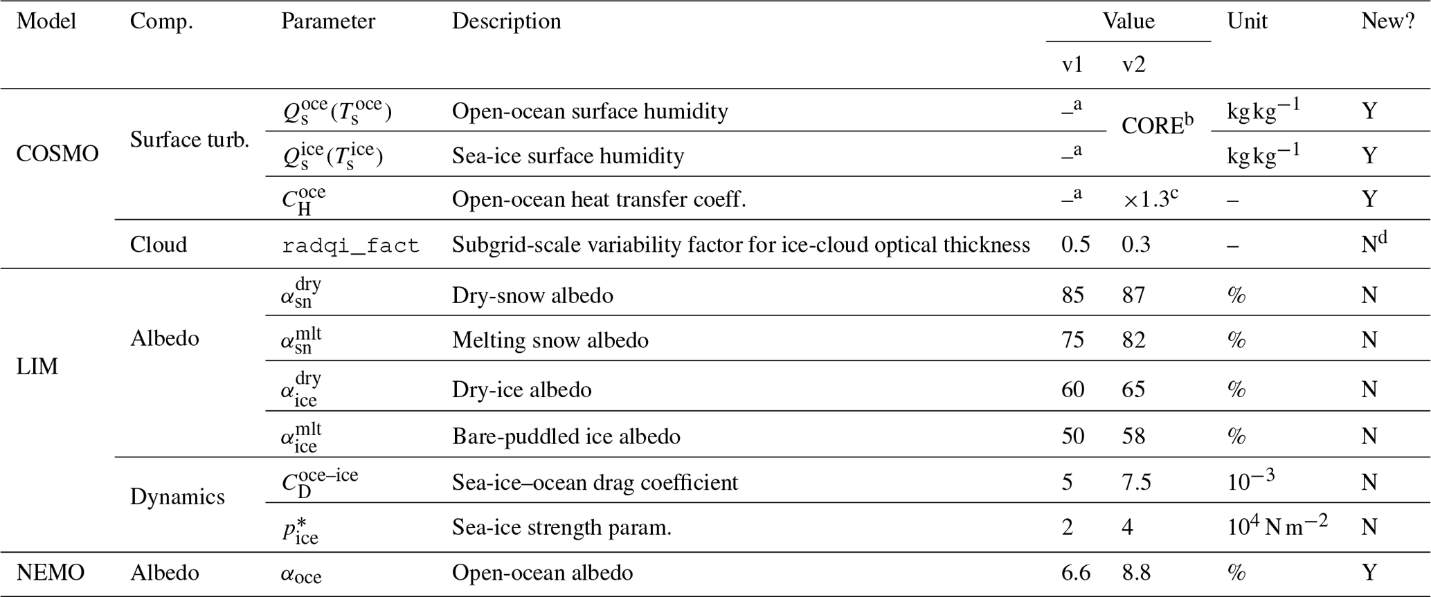
“Comp.”: component; “Surface turb.”: surface turbulence. ^a Regular COSMO scheme. ^b Surface humidity diagnostics from CORE bulk formula (Large and Yeager, 2004). ^c Regular COSMO scheme value increased by 30 %. ^d Adapted from Muskatel et al. (2021).

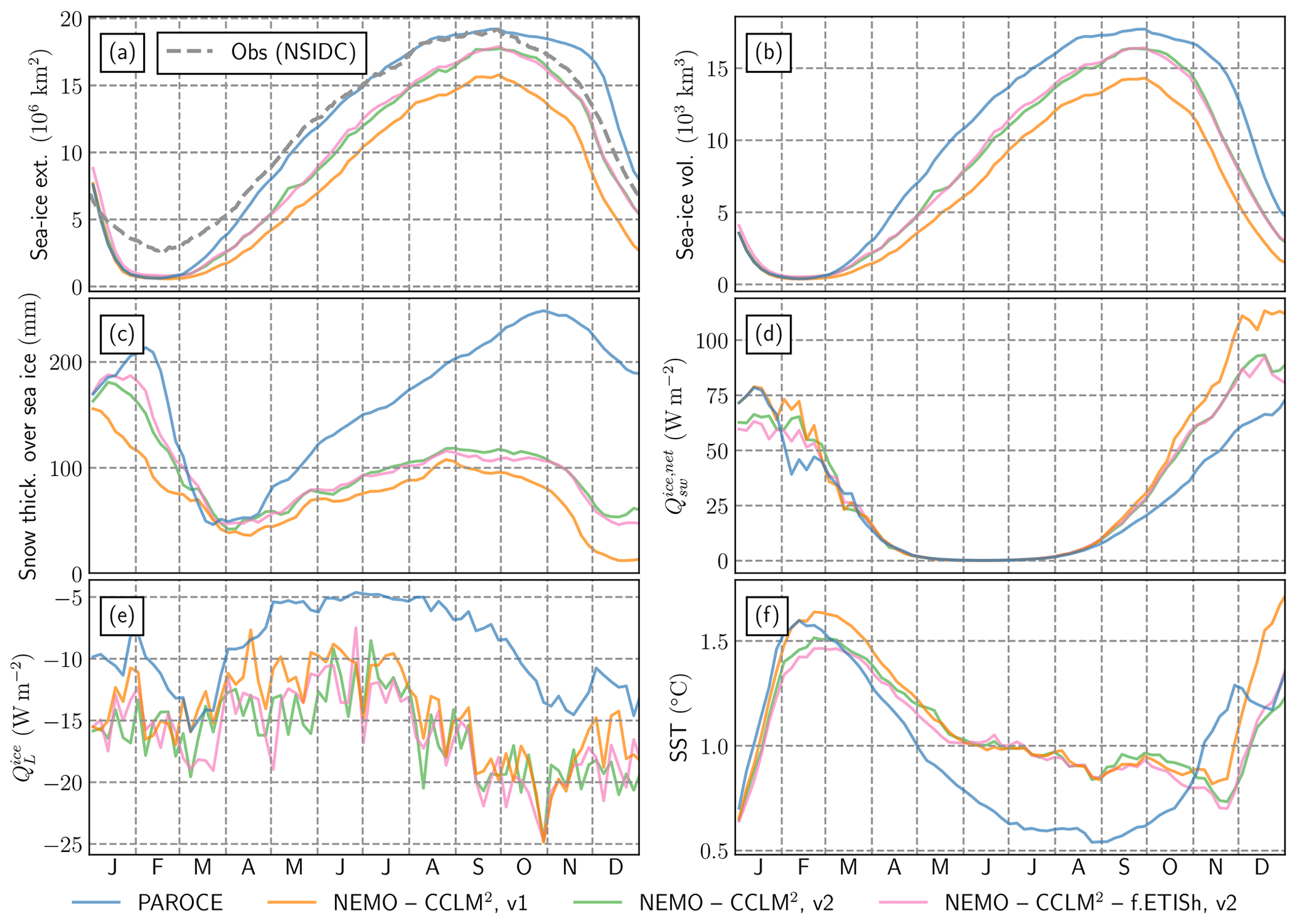
Figure E1 Integrated diagnostics from several PARASO tuning experiments: (a) sea-ice extent (also featuring observations from Fetterer et al., 2017); (b) sea-ice volume; (c) average snow thickness over sea ice (only sea-ice-covered cells counted); (d) net downward surface solar radiation over sea ice; (e) downward latent heat flux over sea ice; (f) average SSTs (only sea-ice-free cells counted). Panels (c), (d) and (e) are averaged over all sea-ice-covered cells. Panel (f) is averaged over all sea-ice-free cells south of 55^∘S. Sea-ice coverage has been defined with a 15 % concentration threshold. Results shown above are all from 1 year (2000) of experiments.

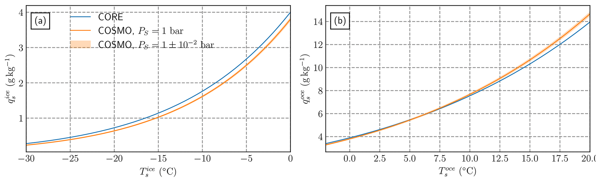
Figure E2 Comparison in surface moisture diagnostics (i.e., T_s↦Q_s(T_s)) over (a) sea ice and (b) open ocean for the COSMO and the CORE (Large and Yeager, 2004) parameterizations.

One of the most significant problems that has been encountered when coupling NEMO and CCLM², compared to NEMO stand-alone experiments, is the degraded snow cover over sea ice. While the increase in surface albedo does slightly counterbalance the degraded snow cover, this aspect remains problematic in PARASO. Compared with the CORE bulk formula used in NEMO, systematic biases in surface humidity have been identified (dry bias for sea ice, moist bias for open ocean; see Fig. E2). Theoretically, the dry bias over sea ice may partly be responsible for the enhanced evaporation, yet correcting it by using the CORE humidity diagnostics only yielded slightly perceivable improvements. The COSMO heat and moisture transfer coefficient (same coefficient) has also been slightly increased to further prevent biases related to latent heat, but once again, this only yielded slight improvements. This was to be expected, as the excess in latent heat is probably related to a moist bias in the near-surface atmosphere: hence, tuning the moisture transfer coefficients only affects the speed at which the evaporation bias develops at the ocean surface, without altering the longer-term bias from developing.

All surface albedo values were slightly increased in order to limit the ocean surface warming (and sea-ice decline) that was observed in PARASO. While we admit that this was solely done to counterbalance the PARASO warm biases, the values used are all within the observational range. Moreover, default LIM3 sea-ice albedo parameters had mostly been tuned for Arctic simulations, suggesting that some Southern Ocean adaptations may indeed be required.

Finally, sea-ice dynamical properties were also slightly retuned to limit sea-ice compaction related to the relatively strong PARASO winds. One signature of this phenomenon is the relatively small bias in sea-ice volume (see Fig. 8b) compared to extent: the PARASO sea-ice pack is small in area but significant in volume; hence, it is quite thick (see Fig. A7). While the increase of these sea-ice dynamical parameters is quite significant (+50 %), the uncertainty of their actual value is also quite high (Tsamados et al., 2014; Ungermann et al., 2017).