the Creative Commons Attribution 4.0 License.
the Creative Commons Attribution 4.0 License.
 | 20 Jul 2022
Improving Madden–Julian oscillation simulation in atmospheric general circulation models by coupling with a one-dimensional snow–ice–thermocline ocean model
Wan-Ling Tseng
Huang-Hsiung Hsu
Yung-Yao Lan
Wei-Liang Lee
Chia-Ying Tu
Pei-Hsuan Kuo
Ben-Jei Tsuang
Hsin-Chien Liang
A one-column, turbulent, and kinetic-energy-type ocean mixed-layer model (snow–ice–thermocline, SIT), when coupled with three atmospheric general circulation models (AGCMs), yields superior Madden–Julian oscillation (MJO) simulations. SIT is designed to have fine layers similar to those observed near the ocean surface; therefore, it can realistically simulate the diurnal warm layer and cool skin. This refined discretization of the near-surface ocean in SIT provides accurate sea surface temperature (SST) simulation, and thus facilitates realistic air–sea interaction. Coupling SIT with the European Centre/Hamburg Model version 5, the Community Atmosphere Model version 5, and the High-Resolution Atmospheric Model significantly improved MJO simulation in three coupled AGCMs compared to the AGCM driven by a prescribed SST. This study suggests two major improvements to the coupling process. First, during the preconditioning phase of MJO over the Maritime Continent (MC), the often underestimated surface latent heat bias in AGCMs can be corrected. Second, during the phase of strongest convection over the MC, the change in intraseasonal circulation in the meridional circulation enhancing near-surface moisture convergence is the dominant factor in the coupled simulations relative to the uncoupled experiments. The study results show that a fine vertical resolution near the surface, which better captures temperature variations in the upper few meters of the ocean, considerably improves different models with different configurations and physical parameterization schemes; this could be an essential factor for accurate MJO simulation.
- Article
(3765 KB) - Full-text XML
-
Supplement
(1293 KB) - BibTeX
- EndNote


The Madden–Julian Oscillation (MJO) is the dominant pattern of atmospheric intraseasonal variability in the tropics (Madden and Julian, 1972; Zhang, 2005; Jiang et al., 2020). It has been reported that the MJO convection is often observed over sea surface temperature (SST) of greater than 28 ∘C in the Indo-Pacific warm pool (Salby and Hendon, 1994). MJO is an eastward-propagating ocean–atmosphere and convection–circulation coupled phenomenon that lasts for 20–100 d. On these timescales, low-level moisture convergence, warm SST, and shallow upper-ocean mixed-layer depth precede the eastward propagation of organized deep convection by approximately 10 d, with opposite conditions following approximately 10 d afterwards (Krishnamurti et al., 1988; Hendon and Salby, 1994; Woolnough et al., 2000). Heat flux exchange between the atmosphere and ocean modulates the intraseasonal oscillation (Shinoda and Hendon, 1998). Studies have emphasized the importance of moisture and heat flux feedback in MJO (Sobel et al., 2008, 2010; DeMott et al., 2015). Besides, oceanic wave dynamics are suggested to be associated with MJO (e.g., zonal wind stress anomalies driven by the MJO-forced, eastward-propagating, oceanic equatorial Kelvin wave; Hendon et al., 1998; Webber et al., 2010), and the signals could extend as deep as 1500 m in the ocean (Matthews et al., 2007). Furthermore, the westward-propagating, oceanic, equatorial Rossby wave can initiate the next MJO in the Indian Ocean (Webber et al., 2010, 2012). Evidence of oceanic intraseasonal signals coupling with atmospheric signals was observed in terms of the sea level, surface heat flux, salinity, and temperature during field experiments and in situ monitoring (Oliver and Thompson, 2011; Drushka et al., 2012; Wang et al., 2013; Chi et al., 2014; Matthews et al., 2014; DeMott et al., 2015; Fu et al., 2015).
Recent modeling studies have demonstrated that most coupled models could improve MJO simulations, but the ocean, driven by the atmosphere, contributes indirectly by improving the mean state, heat flux, fresh water, and momentum. DeMott et al. (2016) estimated that direct SST-driven ocean feedback contributes to the MJO propagation of up to 10 % by a change in column moisture. A comparison of the direct and indirect effects of SST indicated that direct effects, such as SST-driven surface fluxes, tend to offset wind-driven fluxes (DeMott et al., 2015, 2016, 2019). The factor of indirect ocean feedback on the atmospheric physical process includes strong MJO convection, which can amplify the radiative feedback to MJO convections associated with large cloud systems (Del Genio and Chen, 2015). The SST gradients can drive the MJO low-level convergence (Hsu and Li, 2012; Li and Carbone, 2012) and destabilize lower tropospheric conditions to further enhance low-level convergence to the east of the MJO convergence (Wang and Xie, 1998; Marshall et al., 2008; Benedict and Randall, 2011; Fu et al., 2015). Many observational and model studies have reported that coupled feedback enhances the MJO with strong horizontal moisture advection, driven by sharp mean near-equatorial meridional moisture gradients (DeMott et al., 2015; Jiang et al., 2018; DeMott et al., 2019; Jiang et al., 2020). These findings suggest that high-frequency SST perturbations could improve moisture convergence efficiency and enhance MJO propagation through relatively smooth background moisture distribution.
Tseng et al. (2015) identified the key role of the upper-ocean warm layer in improving the MJO eastward propagation simulation using the European Centre/Hamburg Model version 5 (ECHAM5), coupled with the one-column ocean model named snow–ice–thermocline (SIT). Many observational (Drushka et al., 2012; Chi et al., 2014) and modeling (Klingaman and Woolnough, 2013; DeMott et al., 2019; Klingaman and Demott, 2020) studies have supported this hypothesis. However, coupling the SIT to only one atmospheric general circulation model (AGCM) may be insufficient to prove the effectiveness of the coupling. In this study, we coupled the SIT to three AGCMs: ECHAM5, the Community Atmosphere Model version 5 (CAM5), and the High-Resolution Atmospheric Model (HiRAM). We also discussed the coupling mechanism that leads to simulation improvement.
The remainder of the paper is organized as follows. In Sect. 2, we describe the models, experimental designs, and observational data. Sections 3 and 4 present the results and discussion, respectively.
2.1 Observational, atmospheric, and oceanic data
Observational data used in this study include precipitation from the Global Precipitation Climatology Project version 1.3 (GPCP, 1∘ resolution, 1997–2010; Adler et al., 2003), outgoing longwave radiation (OLR, 1∘ resolution, 1997–2010; Liebmann, 1996), and daily SST (optimum interpolated SST, OISST, 0.25∘ resolution, 1989–2010; Banzon et al., 2014.) from the National Oceanic Atmosphere Administration. The in situ ocean temperature profiles from 1989 to 2010 were obtained from the Tropical Ocean Global Atmosphere program (McPhaden et al., 2010).
Atmospheric variables were obtained from the European Centre for Medium-range Weather Forecast Reanalysis (ERA-Interim, Dee et al., 2011) from 1989 to 2010. The variables include zonal wind, meridional wind, temperature, specific humidity, sea level pressure, geopotential high, latent heat, sensible heat, and shortwave and longwave radiation. Oceanic temperature data from 1989 to 2010 were obtained from the NCEP Global Ocean Data Assimilation System (GODAS) (Behringer and Xue, 2004) provided by NOAA/OAR/ESRL PSL (Boulder, Colorado, USA; https://psl.noaa.gov/data/gridded/data.godas.html, last access: 11 August 2020).
2.2 Model experiments
In this study, we coupled the one-column ocean model SIT (Tu and Tsuang, 2005; Tsuang et al., 2009) to three AGCMs. SIT simulates variations in the SST and upper-ocean temperature, including the diurnally varying cool skin and warm layer in the upper few meters of the ocean and the turbulent kinetic energy (TKE; Gaspar et al., 1990) in the water column (Tsuang et al., 2001; Tu and Tsuang, 2005; Tu, 2006; Tsuang et al., 2009; Tseng et al., 2015; Lan et al., 2021a). Cool skin is a very thin layer that has a direct contact with the atmosphere, and the warm layer is the warmer sea water immediately below the cool skin in the top few meters of the ocean. They fluctuate diurnally in response to atmospheric forcing. SIT with high vertical resolution realistically simulates the warm layer (within top 10 m) and cool skin (the top layer with 0.001 m thickness) and improves the simulation of upper-ocean temperature (Tu and Tsuang, 2005; Tsuang et al., 2009). The model has been verified at a tropical ocean site (Tu and Tsuang, 2005), in the South China Sea (Lan et al., 2010), and Caspian Sea (Tsuang et al., 2001). The melt and formation of snow and ice above a water column have also been introduced (Tsuang et al., 2001). The three AGCMs used in this study are as follows. ECHAM5, the fifth-generation AGCM developed at the Max Planck Institute for Meteorology (Roeckner et al., 2003, 2006), is a spectral model that employs the Nordeng cumulus convective scheme (Nordeng, 1994). We used a horizontal resolution of T63 (approximately 2∘) with 31 vertical layers and a model top at 10 hPa (approximately 30 km). The second model is the NCAR Community Atmospheric Model version 5 (Hurrell et al., 2013) from the National Center for Atmospheric Research. We used a horizontal resolution of approximately 1.875∘ latitude × 2.5∘ longitude and 30 vertical layers with the Zhang–McFarlane deterministic convection scheme (Zhang and McFarlane, 1995) and the University of Washington shallow convection scheme (Park and Bretherton, 2009). HiRAM was developed based on the Geophysical Fluid Dynamical Laboratory global atmosphere and land model (AM2, Team et al., 2004; Zhao et al., 2009) with a few modifications (Chen et al., 2019). We used a horizontal resolution of 0.5∘ latitude × 0.5∘ longitude with 32 vertical levels. For the boundary layer and free atmospheric turbulence, the model adopted the 2.5-order parameterization of Mellor and Yamada (1982). Surface fluxes are computed based on the Monin–Obukhov similarity theory, given the atmospheric model's lowest level of wind, temperature, and moisture.
There are 42 vertical layers in SIT, with 12 layers in the upper 10 m: the surface, 0.05 mm, 1, 2, 3, 4, 5, 6, 7, 8, 9, and 10 m below the ocean surface. The fine resolution was designed to realistically simulate the upper-ocean warm layer, including a layer at 0.05 mm, reproducing the cool skin of the ocean surface. It is worth noting that coupling a high vertical resolution TKE ocean model with an AGCM is unconventional. To account for neglected horizontal processes, the model ocean was weakly nudged (with a 30 d timescale) to the observed GODAS monthly mean ocean temperature below a depth of 10 m. Nudging was not applied in the upper 10 m. The time step of SIT and AGCMs exchange ocean surface fluxes varying associated with the model resolution, which is 720, 1800, and 900 s in ECHAM-SIT, CAM5-SIT, and HiRAM-SIT, respectively. AGCMs were coupled with the SIT in the tropical region between 30∘ S and 30∘ N and forced by prescribed monthly mean OISST outside this tropical belt.
The experiments comprised three sets of coupled AGCM simulations (ECHAM5-SIT, CAM5-SIT, and HiRAM-SIT) and standalone AGCM simulations forced by observed monthly mean OISST (ECHAM5, CAM5, and HiRAM) from 1985 to 2005. The experiments were designed to evaluate the effect of atmosphere–ocean coupling on MJO simulations. Table 1 presents the model and experiment details.
2.3 Methodology
The analysis focused on the boreal cool season (November–April), which is when the eastward propagation tendency of the MJO is the most prominent. We used the CLIVAR MJO Working Group diagnostics package (CLIVAR, 2009) and a 20–100 d filter to analyze intraseasonal variability. The MJO phase composites were computed using the real-time multivariate MJO index (Wheeler and Hendon, 2004), defined as the leading pair of principal components of intraseasonal OLR, and 850 and 200 hPa zonal winds in the tropics.
The vertically integrated moist static energy (MSE) budget was diagnosed based on the following equation:
where h is the MSE (); u and v are the zonal and meridional velocities, respectively; ω is the vertical pressure velocity; LW and SW are the longwave and shortwave radiation fluxes, respectively; and LH and SH are the latent and sensible surface heat fluxes, respectively. The mass-weighted vertical integration from the surface to 200 hPa is denoted as 〈⋅〉, and the intraseasonal anomalies are represented as 〈⋅〉', which were isolated using a 20–100 d bandpass Lanczos filter (Duchon, 1979).
3.1 MJO simulations: ECHAM5-SIT, CAM5-SIT, and HiRAM-SIT
3.1.1 General structure
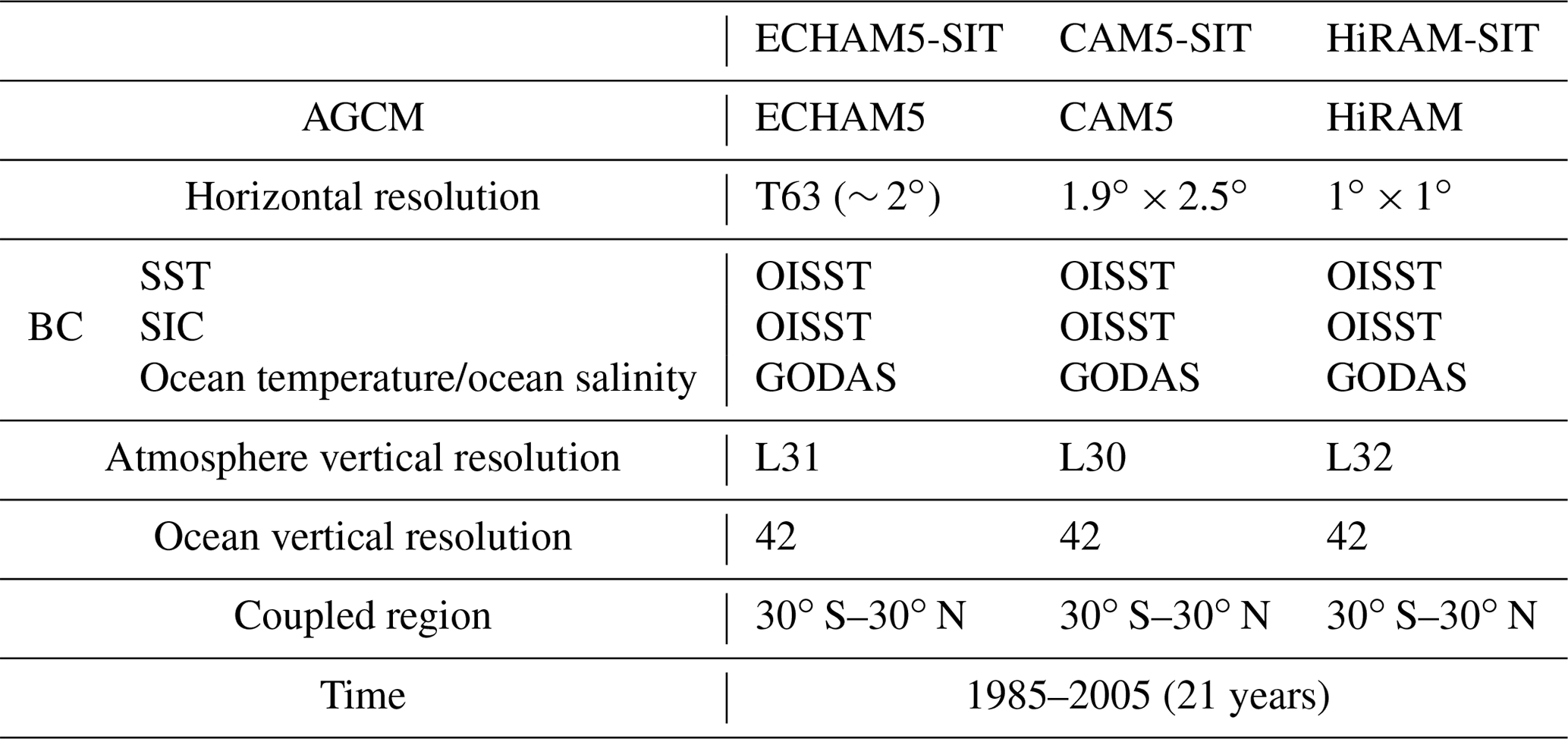
We compared simulated MJO characteristics using three coupled and uncoupled AGCMs. Figure 1 shows the wavenumber–frequency spectra of simulated 850 hPa zonal wind (shading) and precipitation (contours). All three uncoupled AGCMs (hereafter referred to as AGCMs) simulated intraseasonal signals with a lower frequency than was observed and overestimated the westward propagation with periods greater than 80 d (Fig. 1e–g). ECHAM5 and HiRAM simulated signals of wavenumbers 1–3 instead of the observed wavenumber 1 in 850 hPa zonal wind. These results show that all three AGCMs simulated stationary fluctuations with low frequency that were not consistent with the observations. In contrast, coupled AGCMs realistically reproduce the observed spectral characteristics and strength of the eastward propagation at wavenumbers 1 to 2 in 850 hPa zonal wind (Fig. 1b–d). Although HiRAM simulated eastward propagation in a wider frequency spectrum than observed, the coupled model clearly displays improvements in the MJO simulation compared with the stationary intraseasonal fluctuation in the uncoupled simulation. Hovmöller diagrams presented in Fig. 2 illustrate the temporal evolution of 850 hPa zonal wind and precipitation in the tropics in both observations and simulations. All three models simulated either stationary (CAM5 and HiRAM) or weak eastward-propagating (ECHAM5) signals in AGCMs, but they more realistically simulated the eastward propagation of the MJO in the coupled models. However, the propagation in the ECHAM5-SIT is still slightly slower than was observed. The improvement obtained in coupled models suggests that active ocean–atmosphere interaction is crucial for successful MJO simulation.
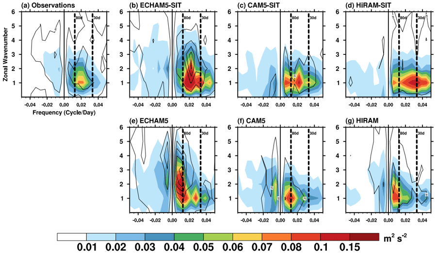
Figure 1Wavenumber–frequency spectra for equatorial 850 hPa zonal wind (shading; m2 s−2) and precipitation (contours; mm2 d−2) over 10∘ S–10∘ N from (a) observations and simulations using the (b–d) coupled and (e–g) uncoupled AGCMs.
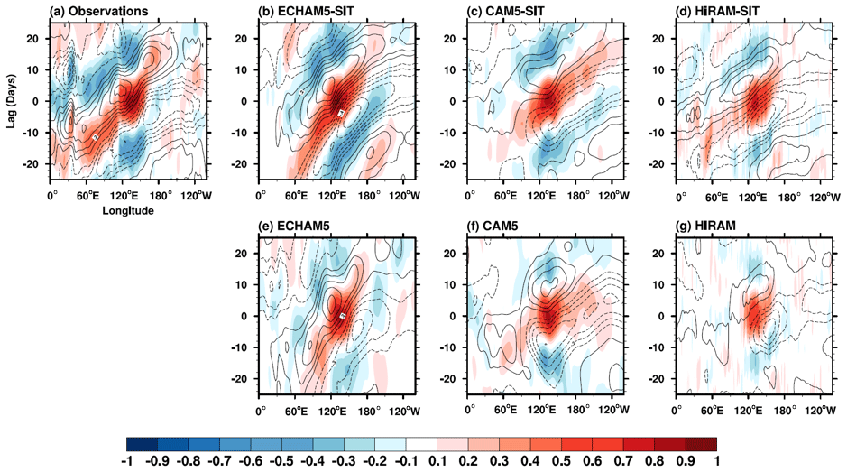
Figure 2The 10∘ S–10∘ N averaged lag–longitude diagrams of intraseasonal precipitation (shading) and 10 m zonal wind (contour) correlated against precipitation (for 10∘ S–5∘ N, 120–150∘ E) from (a) observations and simulations using the (b–d) coupled and (e–g) uncoupled AGCM. The contour interval is 0.1.
3.1.2 Atmospheric and oceanic profiles
The composite MJO life cycle, featuring intraseasonal OLR and 10 m surface wind anomalies for boreal winter in eight phases (following Wheeler and Hendon , 2004), is displayed in Fig. 3. All three coupled models simulated realistic MJO with enhanced circulations and propagation tendency compared to the uncoupled models. The MJO in phase 4, when deep convection is the strongest over the Maritime Continent (MC), demonstrates the large-scale zonally overturning circulation coupling with the convection (Fig. 4). The positive heating region in the coupled experiment is significantly enlarged, deepened, and tilted westward with increasing height compared to those in the uncoupled experiment. Correspondingly, the convective circulation envelope of the MJO is thicker and longitudinally wider in coupled experiments. The strong convection is associated with much enhanced low-level moisture convergence (green contours). Furthermore, the area of positive rainfall anomaly in the coupled experiment becomes larger, and the sea level pressure anomaly is meridionally more confined, exhibiting the characteristics of intensified Kelvin-wave-like perturbations to the east of the deep convection. This enhancement of low-level moisture convergence is consistent with the frictional wave-conditional instability of the second kind of mechanism (Frictional wave CISK; Wang and Rui, 1990; Kang et al., 2013). The enhancement of the Kelvin wave can be observed in the symmetric wavenumber–frequency spectra (Fig. 5). The spectra between 0 and 0.35 d−1 are presented to highlight the MJO and equatorial Kelvin waves. The coherence at wavenumbers of 2–4 for the 10–20 d period is simulated to be stronger in the three coupled models than in the uncoupled models.
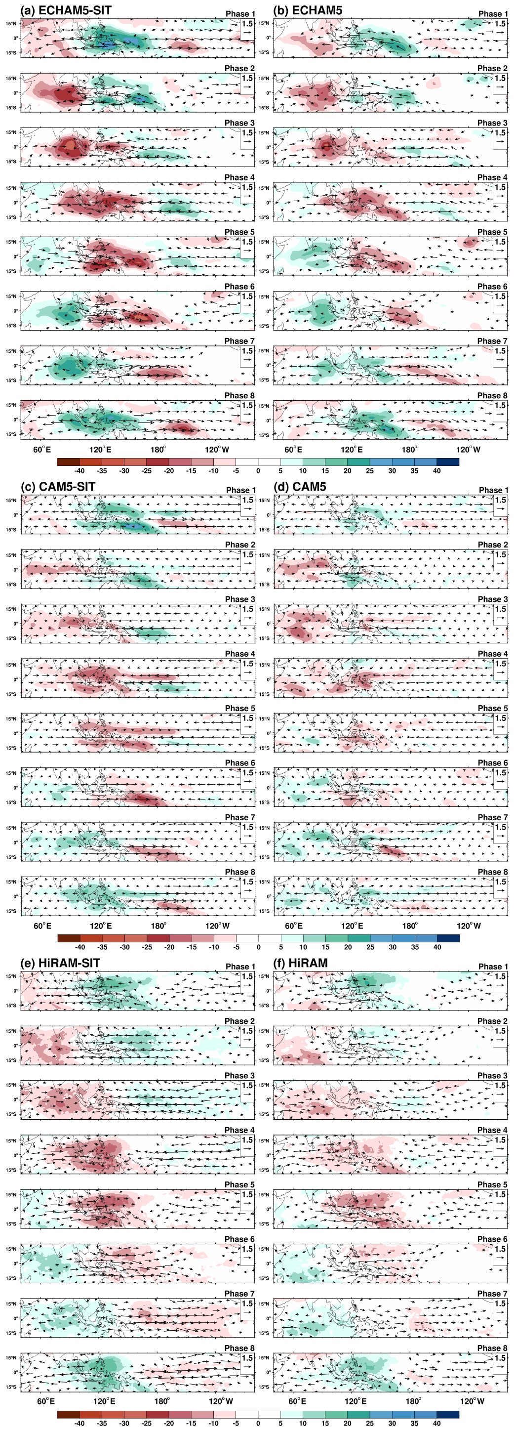
Figure 3Composite November–April 20–100 d OLR (W m−1; shading) and 10 m surface wind anomalies (m s−1; vectors) as a function of the MJO phase in (a) ECHAM5-SIT, (b) ECHAM5, (c) CAM5-SIT, (d) CAM5, (e) HiRAM-SIT, and (f) HiRAM. Vectors <0.6 m s−1 are not shown. The reference vector is shown (in units of m s−1) at the bottom right. The number of days used to generate the composite for each phase is shown to the right of each panel.
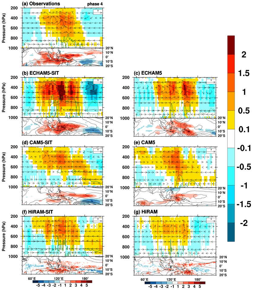
Figure 4Structure of simulated MJO in phase 4. The longitude–height cross sections (averaged over 10∘ S–EQ) of the MJO-scaled wind circulation (vector, u: m s−1; omega: 10−2 Pa s−1), Q1 (shading, unit: K d−1), and the horizontal moisture convergence (green contour, unit: 10−6 g kg−1 s−1) from (a) observations and simulations using the (b–d) coupled and (e–g) uncoupled AGCMs. The contour interval of the moisture convergence is 8 × 10⁻⁶ g kg−1 s−1; the solid line indicates positive values. Precipitation (shading, unit: mm d−1) and sea level pressure (contour, unit: hPa) are also shown. The contour interval of sea level pressure is 30 hPa; the dashed line indicates negative values.

Figure 5Symmetric wavenumber–frequency spectra of 850 hPa zonal wind averaged over 10∘ N–10∘ S using the (a, c, e) coupled and (b, d, f) uncoupled AGCMs (in m2 s−2).
In addition to the atmospheric structure, the SST (Fig. S1) and vertical profile of ocean temperature examined are presented in Fig. 6. The observed SST variation in MJO variability is reproduced well in all three coupled models (Fig. S1). The warm SST leads the main MJO convection by approximately 5–10 d, followed by the cold SST approximately 5–10 d later (Flatau et al., 1997; DeMott et al., 2015; Tseng et al., 2015). Moreover, the observed amplitude fluctuation (approximately 0.5 to 1 ∘C) is realistically simulated. The observed ocean temperature profiles, characterized by the warm layer, along the Equator from the Indian Ocean to the western Pacific are simulated well in the three coupled models (Fig. 6). Meanwhile, simulated temperature anomalies are larger in ECHAM5-SIT than in CAM5-SIT and HiRAM-SIT. Figure S2 shows the fluctuations of observed SST and simulated SST in three sets of coupled and uncoupled models. There is no fluctuation (as expected) in uncoupled simulations, whereas the simulated SST fluctuates with phases similar to those observed at different locations. The amplitudes in ECHAM5-SIT and CAM5-SIT are similar to the observed values, whereas those in HiRAM-SIT seem to be smaller in the western Pacific. The differences between models are likely due to the different atmospheric model configurations because they were otherwise coupled to the same 1-D ocean model. Since the atmosphere is the main driver to extract heat from the ocean, different responses of atmospheric models likely have different effects on SST. Pinpointing the cause of quantitative differences between models will require further detailed analysis. The consistent results in all three coupled models support the conclusion of Tseng et al. (2015) that resolving fine vertical resolution in the upper ocean improves the simulation of the warm layer and MJO propagation and variability. Our results further demonstrate that the effect of atmosphere–ocean coupling on the MJO could be independent of AGCMs with different configurations and atmospheric physical parameterizations and that coupling seems to be a more fundamental approach.

Figure 6Vertical ocean temperature (∘C) profiles with respect to MJO phases for intraseasonal anomalies (i.e., with 20–100 d filtering) in observations and simulations using coupled models. Observations are in line with data from TAO. Because of storage limitations, only 3 and 10 m water temperatures are presented in the HiRAM-SIT simulation.
3.1.3 Performance comparison
Model performance is summarized in Fig. 7. The scatter plot shows the power ratio of east–west-propagating waves (x axis) versus the pattern correlation between the simulated and observed precipitation anomaly in Hovmöller diagrams (Fig. 2; y axis). The east:west ratio was calculated by dividing the eastward-propagating power by the westward-propagating power of 850 hPa zonal wind summed over wavenumbers of 1–2 and a period of 30–80 d. Compared with the observations, coupled simulations (marked by circles) exhibit better simulation than uncoupled simulations (marked by asterisks). A comparison of combined explained variance using real-time multivariate MJO series 1 (RMM1) and 2 (RMM2) (Fig. 7b) based on Wheeler and Hendon (2004) shows marked increases after coupling. The comparison demonstrates that coupling is essential for realistic MJO simulations.
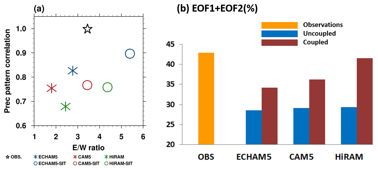
Figure 7Scatter plots of various MJO indices based on observations and experiments (Table 1). (a) The x axis is the power ratio of east–west-propagating waves. The east–west ratio was calculated by dividing the sum of eastward-propagating power by its westward-propagating counterpart within wavenumbers 1–3 (1–2 for zonal wind) and a period of 30–80 d. The y axis is the pattern correlation of precipitation and eastward propagation, as shown in Fig. 2. (b) Sum of RMM1 and RMM2 variances based on Wheeler and Hendon (2004).
3.2 Mechanism discussion
We applied the MSE budget to diagnose the moisture budget associated with the MJO. Figure 8 shows a Hovmöller diagram of MSE tendency averaged from the area between 10∘ S and the Equator and the overlying precipitation anomalies. MSE tendency derived from reanalysis fluctuates in quadrature with precipitation anomaly with positive (negative) MSE tendency, leading (lagging) major convection by approximately one to two phases (DeMott et al., 2015, 2016, 2019). Coupled models simulate stronger eastward propagation in the MSE tendency and precipitation anomalies and realistic phase lag between the two. Stronger MSE tendencies in coupled simulations are observed in ECHAM5 and HiRAM but are less clear in CAM5. Figure 8d, g, and j show the differences between coupled and uncoupled simulations. One notable feature is the positive (negative) MSE tendency preceding positive (negative) precipitation anomaly, which preconditions environments for eastward propagation of active (inactive) convection and associated circulation. Next, we diagnosed the relative contribution of each term in Eq. (1) to the MSE tendency with a focus on the MC, where the largest positive MSE tendency and precipitation anomaly were found.
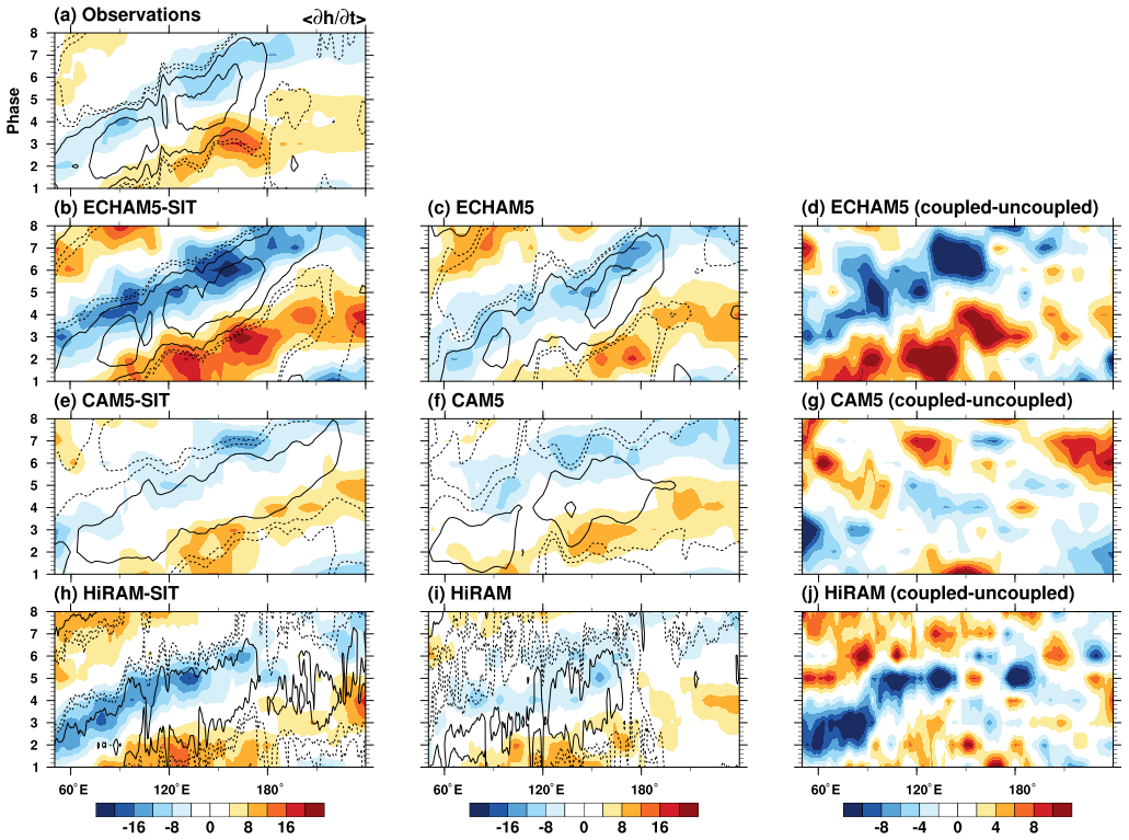
Figure 8Hovmöller diagrams averaged over the area between 10∘ S and the Equator for MSE (shading; J kg−1) and precipitation (contour; mm d−1) composites following the RMM index from (a) observations and simulations using the (b, e, j) coupled and (c, f, k) uncoupled AGCMs and (d, i, l) their difference. The contour interval is precipitation anomalies.
3.2.1 Preconditioning phase
Following the peak MSE tendency over the MC (120–150∘ E) during phase 2 (Fig. 8d, g, and j), values of each term contributing to the column-integrated MSE tendency in Eq. (1) preceding the deep convection over the MC area (10∘ S–0∘ N/S, 120–150∘ E) are shown in Fig. 9. Vertical advection is the dominant term with the major compensation from longwave radiation during phase 2 when convection is still in the eastern Indian Ocean, as identified by Wang and Li (2020). Moreover, the LH term is consistent within all three models and contributes less negative MSE tendency in coupled models than AGCMs. The results show that the contribution comes from the LH term in this early phase stage. The LH effect was overlooked in Tseng et al. (2015) because of the weak MJO variability in coupled simulations. However, this negative LH bias becomes one of the key factors in enhancing the leading MSE tendency during the MJO preconditioning phases. This suggests that the surface latent flux bias in AGCMs can be corrected by involving the coupling process in the preconditioning phase. Generally, coupling improves the budget simulation. The positive contribution of vertical advection and negative contribution of LH in MSE tendency is closer to being realistic in the coupled simulations during the initial phase of the MJO.
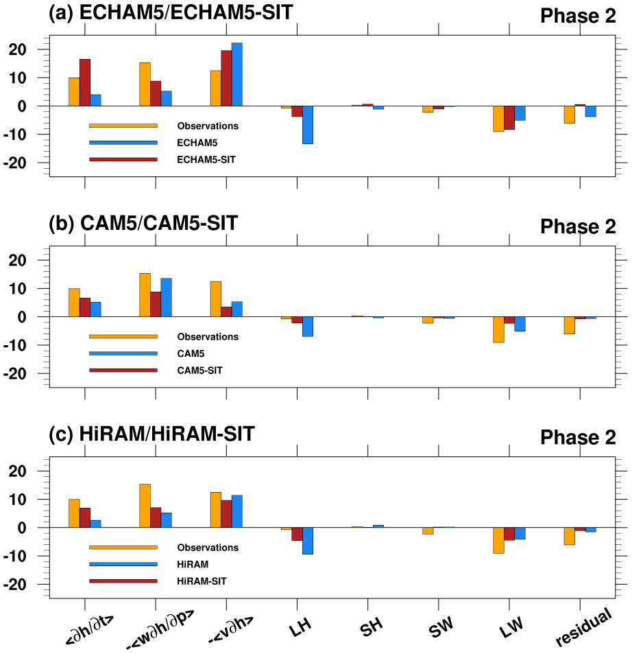
Figure 9Model-simulated column-integrated MSE budget terms (J kg−1 s−1) during phase 2 of the MJO. Black, red, and blue represent the data from the observations, Nordeng scheme simulations, and Tiedtke scheme simulations, respectively. The averaged domain is 10∘ S–0∘ N/S, 120–150∘ E.
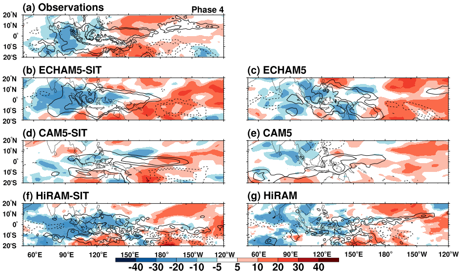
Figure 10Phase 4 of the column-integrated MSE tendency (shading; J kg−1 s−1) and precipitation (contours; mm d−1) based on (a) observations, (b) ECHAM5-SIT, (c) ECHAM5, (d) CAM5-SIT, (e) CAM5, (g) HiRAM-SIT, and (f) HiRAM. The nine-point local smoothing is applied here to the intraseasonal precipitation variance of HiRAM (contours only).
3.2.2 Phase of strongest convection over the MC
We compared the spatial distribution of MSE and precipitation in phase 4 when convection was the strongest in the MC (Fig. 10). In the observations, the main convection occurs in the MC from 90 to 150∘ E. A positive MSE tendency with a maximum value near 10∘ N and 10∘ S is identified in the east of the MJO convection centered near the Equator. Meanwhile, a negative integrated MSE tendency is found in the west of the MJO convection, and the meridionally confined structure near the Equator exhibits the characteristics of the equatorial Kelvin wave embedded in the MJO. Clearly, coupled models outperform uncoupled models in reproducing these signals. To quantify the contribution of coupling to the improvement, we follow Jiang et al. (2018) to project all MSE terms to the observations (Fig. 11). The dominant contribution of horizontal advection to the MSE tendency in the observations (Fig. 11a) is simulated well in the coupled simulations (but not in the uncoupled simulations) of ECHAM5 and CAM5 (Fig. 11b and c). Although a similar dominant effect was observed in both simulation types in HiRAM, it is enhanced in the coupled simulation (Fig. 11d). The horizontal advection term is further decomposed into zonal and meridional components (Fig. 11e–h); both components have a positive contribution, but the meridional component has a larger amplitude. Furthermore, the uncoupled ECHAM5 and CAM5 models simulate unrealistic features: positive contribution from zonal advection but negative contribution from meridional advection. In contrast, coupled models simulate the dominance of meridional advection well. In HiRAM, the uncoupled model simulates almost equally positive contributions from both terms. However, the coupled model simulates a larger contribution from meridional advection. We further decompose the meridional advection to assess the relative contributions of an intraseasonal perturbation and the mean state. Consistent with the observations (Fig. 11i), the meridional advection by intraseasonal flow () is the main factor in improving the simulations in the coupled models (Fig. 11j–l). Our results are consistent with those of Jiang et al. (2018). To evaluate the relative contribution of intraseasonal circulation and background moisture, we further diagnosed changes in at phase 4. Here the overbar shows that the time mean and prime represents intraseasonal anomaly. Changes in the MJO meridional advection term for coupled experiments relative to uncoupled can be written as follows:
where Δ represents the coupled–uncoupled change. The terms (a)–(c) in Eq. (2) are presented as bar charts in Fig. 12. The change in the intraseasonal circulation in the meridional circulation is the dominant factor in coupled simulations relative to uncoupled experiments. The instantaneous SST horizontal distribution dominates this moisture budget change due to the atmosphere–ocean coupling effect. Therefore, the change of varying moisture induces the intraseasonal circulation change. The results confirm that the dominance of dynamic influence over thermodynamic response to atmosphere–ocean coupling is essential in improving MJO simulations.

Figure 11(a–d) The relative role of each MSE component of phase 4 through the projection of the spatial pattern of each MSE budget over the MC (domain) onto the total MSE tendency pattern (Fig. 8a). (e–h) Decomposite of the total horizontal MSE advection based on zonal and meridional components. (i–l) Relative role of the meridional horizontal MSE advection based on the MJO circulation and the mean state of moisture.
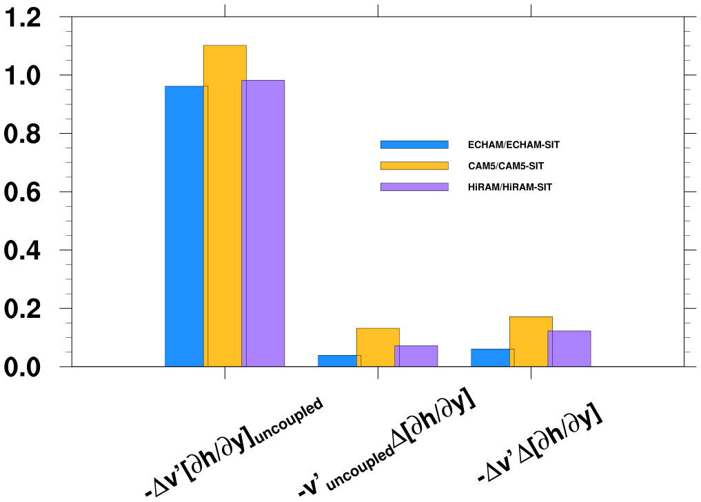
Figure 12Bar chart of the relative contribution of intraseasonal convergence and background moisture between the coupled and uncoupled changes in MJO phase 4.
3.3 Discussion: mean state and intraseasonal variance
We examined the simulated mean state, which has been suggested a key factor affecting MJO simulations (Inness et al., 2003; Watterson and Syktus, 2007; Kim et al., 2009, 2011, 2014; Jiang et al., 2018, 2020). The three models exhibited different tropical SST responses to coupling (Fig. S3e). Over the warm pool area, CAM-SIT and HiRAM-SIT underestimate the SST, whereas ECHAM5-SIT overestimates the SST. Note that warm SST bias in the eastern tropical Pacific was simulated in the three models due to the lack of oceanic circulation in the SIT. The simulated zonal wind in the three models (Fig. S3b–d) demonstrated different responses to coupling. Figure S2c show the 850 hPa zonal wind differences between coupled and uncoupled models (shading) and the total field in uncoupled models (contours). Figure S3f–h show the 10∘ S–0∘ N/S averaged 850 hPa zonal wind in the coupled and uncoupled models. In ECHAM5-SIT, the westerly wind is slightly enhanced in the eastern Indian Ocean but decreases in the western Indian Ocean and western Pacific Ocean. In CAM5-SIT, westerly wind reduces in the Indian Ocean but enhances over the western Pacific. HiRAM-SIT has similar changes to those in ECHAM5-SIT, i.e., it decreases over the MC area but increases in the western Indian Ocean and Pacific. Generally, the three models disagree on the zonal wind mean state changes in response to coupling.
The mean moisture changes are substantially enhanced over the tropical areas in ECHAM5 after coupling (Fig. S4b and e). However, in CAM5 and HiRAM no clear change was observed to the south of the Equator, but strong drying was observed to the north for the same models (Fig. S4c, d, f, and g). The only common feature among the three models is the enhanced meridional gradient of mean moisture, which is consistent with many previous studies (Kim et al., 2014; Jiang et al., 2018; Ahn et al., 2020). Our budget analysis demonstrated that the meridional transport by the intraseasonal meridional circulation is the dominant term. It also showed that the meridional gradient of mean moisture is the secondary effect in enhancing MJO simulations by coupling. After coupling, the mean precipitation changes are more consistent among the three models (Fig. S5). One of the major changes is the southward shift of the major precipitation zone, resulting in precipitation increases over the regions south of the Equator (except in the MC). Similarly, the precipitation intraseasonal variance (20–100 d filtered) was markedly enhanced in these regions (Fig. S6). ECHAM5-SIT exhibits a relatively minor increase over the western MC. In contrast, HiRAM-SIT exhibits the strongest enhancement, particularly in the Indian Ocean. Generally, all three coupled models enhance the intraseasonal signals over the tropics with discrepancies in their level of detail. Meanwhile, the model mean state does not substantially improve after coupling. Thus, in this study, the mean state is not the main contribution to enhancing the MJO simulation after coupling. Instead, coupling leading to rigorous atmosphere–ocean interaction on intraseasonal timescales is likely the reason for the improving MJO simulation.
This study used a one-column, TKE-type ocean mixed-layer model (SIT) coupled with AGCMs to improve MJO simulation. SIT is designed to have fine layers near the surface that simulate the warm layer, cool skin, and diurnal fluctuations well. This refined discretization under the ocean surface in SIT provides improved SST simulation, which provides a more realistic air–sea interaction. Coupling SIT with ECHAM5, CAM5, and HiRAM significantly improves the MJO simulation in the three AGCMs compared with that of the prescribed SST-driven AGCMs. The vertical cross section indicates that the strengthened low-level convergence during the preconditioning phase is better simulated in the coupled experiment. Furthermore, the phase variation and amplitude of the SST and ocean temperature under the surface can be realistically simulated. Our results reveal that the MJO can be realistically simulated in terms of strength, period, and propagation speed by increasing the vertical resolution of the one-column ocean model to better resolve the upper-ocean warm layer.
The MSE budget analysis revealed that the coupling effects during the preconditioning and mature phases exhibit different contributions. During the preconditioning phase, the positive contribution of vertical advection and the negative contribution of LH in MSE tendency are closer to realistic values in coupled simulations during the initial phase of the MJO. Additionally, the meridional component of the horizontal advection term is the dominant term during the mature phase of the strongest convection in the MC, enhancing the simulation after coupling. Improved meridional circulation is essential in the coupled simulations that outperformed uncoupled experiments. The results confirm that the dominance of dynamic influence over thermodynamic influence in response to the atmosphere–ocean coupling is the key process in improving MJO simulations. In summary, this study suggests two major enhancements of the coupling process. First, the underestimated surface LH bias in AGCMs can be corrected during the preconditioning phase of the MJO over the MC. Second, during the strongest convection phase over the MC, the change in intraseasonal circulation in the meridional circulation is the dominant factor in coupled simulations relative to uncoupled experiments. Although many studies have indicated the key role played by the mean state, the mean state in our simulations provides only a secondary contribution to enhancing the MJO simulation, with coupling being the main contributor. For example, zonal wind and precipitation changed inconsistently in the three models after coupling. Instead, the meridional gradient of the mean moisture and intraseasonal precipitation variance has a better relationship after coupling. Therefore, coupling leading to rigorous atmosphere–ocean interaction in the intraseasonal time scale, but no change in mean states, is likely the reason for MJO simulation improvement. This study supports previous findings (Tseng et al., 2015) that show that enhancing atmosphere–ocean coupling by considering an extremely high vertical resolution in the first few meters of the ocean model improves MJO simulations. It also supports that this improvement is independent of AGCMs with different configurations and physical parameterization schemes. Resolving the atmosphere–ocean coupling may be more beneficial than modifying the atmospheric physical parameterization schemes in general circulation models. In brief, this study suggested the effectiveness of air–sea coupling for improving MJO simulation in a climate model and demonstrated the critical effect that being able to simulate the warm layer has on the results. Additionally, the findings presented here enhance our understanding of the physical processes that shape the characteristics of the MJO.
The model code of CAM5–SIT, ECHAM5-SIT, and HiRAM-SIT is available at https://doi.org/10.5281/zenodo.5701538 (Tseng, 2021), https://doi.org/10.5281/zenodo.5510795 (Lan et al., 2021b), and https://doi.org/10.5281/zenodo.5701579 (Tu, 2021), respectively. Observational data used in this study include precipitation from Global Precipitation Climatology Project V1.3 (GPCP, 1∘ resolution), OLR (1∘ resolution), and daily SST (Optimum Interpolated SST, 0.25∘ resolution) from the National Oceanic and Atmosphere Administration, and variables were obtained from the European Centre for Medium-range Weather Forecast Reanalysis (ERA-Interim). All experiments were conducted at the National Center for High-Performance Computing. All model code and data presented here can be obtained by contacting the first author, Wan-Ling Tseng (wtseng@ntu.edu.tw).
The supplement related to this article is available online at: https://doi.org/10.5194/gmd-15-5529-2022-supplement.
HHH and WLT conceptualized the study, analyzed the data, and wrote the manuscript. YYL, WLL, PHK, BJT, CYT, and HCL developed the model and provided the simulations.
The contact author has declared that none of the authors has any competing interests.
Publisher's note: Copernicus Publications remains neutral with regard to jurisdictional claims in published maps and institutional affiliations.
This work was supported by the Taiwan Ministry of Science and Technology (grant nos. MOST 109-2111-M-001-012-MY3, MOST 110-2811-M-001-633, and MOST 110-2123-M-001-003). We are grateful to the National Center for High-Performance Computing for providing computer facilities. The Max Planck Institute for Meteorology provided ECHAM5.4. We sincerely thank the National Center for Atmospheric Research and their Atmosphere Model Working Group for release CESM1.2.2. This paper was edited by Wallace Academic Editing and Enago.
This research has been supported by the Ministry of Science and Technology, Taiwan (grant nos. MOST 109-2111-M-001-012-MY3, MOST 110-2811-M-001-633, and MOST 110-2123-M-001-003).
This paper was edited by Richard Neale and reviewed by two anonymous referees.
Adler, R. F., Huffman, G. J., Chang, A., Ferraro, R., Xie, P.-P., Janowiak, J., Rudolf, B., Schneider, U., Curtis, S., and Bolvin, D.: The version-2 global precipitation climatology project (GPCP) monthly precipitation analysis (1979–present), J. Hydrometeorol., 4, 1147–1167, 2003.
Ahn, M. S., Kim, D., Kang, D., Lee, J., Sperber, K. R., Gleckler, P. J., Jiang, X., Ham, Y. G., and Kim, H.: MJO propagation across the Maritime Continent: Are CMIP6 models better than CMIP5 models?, Geophys. Res. Lett., 47, e2020GL087250, https://doi.org/10.1029/2020GL087250, 2020.
Banzon, V. F., Reynolds, R. W., Stokes, D., and Xue, Y.: A -spatial-resolution daily sea surface temperature climatology based on a blended satellite and in situ analysis, J. Climate, 27, 8221–8228, 2014.
Behringer, D. and Xue, Y.: Evaluation of the global ocean data assimilation system at NCEP: The Pacific Ocean, Proc. Eighth Symp. on Integrated Observing and Assimilation Systems for Atmosphere, Oceans, and Land Surface, http://origin.cpc.ncep.noaa.gov/products/people/yxue/pub/13.pdf (last access: 11 August 2020), 2004.
Benedict, J. J. and Randall, D. A.: Impacts of Idealized Air–Sea Coupling on Madden–Julian Oscillation Structure in the Superparameterized CAM, J. Atmos. Sci., 68, 1990–2008, https://doi.org/10.1175/jas-d-11-04.1, 2011.
Chen, C.-A., Hsu, H.-H., Hong, C.-C., Chiu, P.-G., Tu, C.-Y., Lin, S.-J., and Kitoh, A.: Seasonal precipitation change in the western North Pacific and East Asia under global warming in two high-resolution AGCMs, Clim. Dynam., 53, 5583–5605, 2019.
Chi, N. H., Lien, R. C., D'Asaro, E. A., and Ma, B. B.: The surface mixed layer heat budget from mooring observations in the central Indian Ocean during Madden–Julian Oscillation events, J. Geophys. Res.-Oceans, 119, 4638–4652, 2014.
CLIVAR Madden–Julian Oscillation Working Group: MJO Simulation Diagnostics, J. Climate, 22, 3006–3030, 2009.
Dee, D., Uppala, S., Simmons, A., Berrisford, P., Poli, P., Kobayashi, S., Andrae, U., Balmaseda, M., Balsamo, G., and Bauer, P.: The ERA-Interim reanalysis: Configuration and performance of the data assimilation system, Q. J. Roy. Meteor. Soc., 137, 553–597, 2011.
Del Genio, A. D. and Chen, Y.: Cloud-radiative driving of the Madden-Julian oscillation as seen by the A-Train, J. Geophys. Res.-Atmos., 120, 5344–5356, https://doi.org/10.1002/2015JD023278, 2015.
DeMott, C. A., Klingaman, N. P., and Woolnough, S. J.: Atmosphere-ocean coupled processes in the Madden-Julian oscillation, Rev. Geophys., 53, 1099–1154, 2015.
DeMott, C. A., Benedict, J. J., Klingaman, N. P., Woolnough, S. J., and Randall, D. A.: Diagnosing ocean feedbacks to the MJO: SST-modulated surface fluxes and the moist static energy budget, J. Geophys. Res.-Atmos., 121, 8350–8373, 2016.
DeMott, C. A., Klingaman, N. P., Tseng, W. L., Burt, M. A., Gao, Y., and Randall, D. A.: The convection connection: How ocean feedbacks affect tropical mean moisture and MJO propagation, J. Geophys. Res.-Atmos., 124, 11910–11931, 2019.
Drushka, K., Sprintall, J., Gille, S. T., and Wijffels, S.: In situ observations of Madden-Julian Oscillation mixed layer dynamics in the Indian and western Pacific Oceans, J. Climate, 25, 2306–2328, 2012.
Duchon, C. E.: Lanczos filtering in one and two dimensions, J. Appl. Meteorol. Clim., 18, 1016–1022, 1979.
Flatau, M., Flatau, P. J., Phoebus, P., and Niiler, P. P.: The feedback between equatorial convection and local radiative and evaporative processes: The implications for intraseasonal oscillations, J. Atmos. Sci., 54, 2373–2386, 1997.
Fu, X., Wang, W., Lee, J.-Y., Wang, B., Kikuchi, K., Xu, J., Li, J., and Weaver, S.: Distinctive roles of air–sea coupling on different MJO events: A new perspective revealed from the DYNAMO/CINDY field campaign, Mon. Weather Rev., 143, 794–812, 2015.
Gaspar, P., Gregoris, Y., and Lefevre, J.-M.: A simple eddy kinetic energy model for simulations of the oceanic vertical mixing: Tests at station Papa and long-term upper ocean study site, J. Geophys. Res.-Oceans, 95, 16179–16193, 1990.
Hendon, H. H. and Salby, M. L.: The life cycle of the Madden-Julian oscillation, J. Atmos. Sci., 51, 2225–2237, 1994.
Hendon, H. H., Liebmann, B., and Glick, J. D.: Oceanic Kelvin waves and the Madden–Julian oscillation, J. Atmos. Sci., 55, 88–101, 1998.
Hsu, P.-C. and Li, T.: Role of the Boundary Layer Moisture Asymmetry in Causing the Eastward Propagation of the Madden-Julian Oscillation, J. Climate, 25, 4914–4931, 2012.
Hurrell, J. W., Holland, M. M., Gent, P. R., Ghan, S., Kay, J. E., Kushner, P. J., Lamarque, J.-F., Large, W. G., Lawrence, D., and Lindsay, K.: The community earth system model: a framework for collaborative research, B. Am. Meteorol. Soc., 94, 1339–1360, 2013.
Inness, P. M., Slingo, J. M., Guilyardi, E., and Cole, J.: Simulation of the Madden-Julian Oscillation in a coupled general circulation model. Part II: The role of the basic state, J. Climate, 16, 365–382, 2003.
Jiang, X., Adames, Á. F., Zhao, M., Waliser, D., and Maloney, E.: A unified moisture mode framework for seasonality of the Madden–Julian oscillation, J. Climate, 31, 4215–4224, 2018.
Jiang, X., Adames, Á. F., Kim, D., Maloney, E. D., Lin, H., Kim, H., Zhang, C., DeMott, C. A., and Klingaman, N. P.: Fifty years of research on the Madden-Julian Oscillation: Recent progress, challenges, and perspectives, J. Geophys. Res.-Atmos., 125, e2019JD030911, https://doi.org/10.1029/2019JD030911, 2020.
Kang, I.-S., Liu, F., Ahn, M.-S., Yang, Y.-M., and Wang, B.: The Role of SST Structure in Convectively Coupled Kelvin-Rossby Waves and Its Implications for MJO Formation, J. Climate, 26, 5915–5930, 2013.
Kim, D., Sperber, K., Stern, W., Waliser, D., Kang, I.-S., Maloney, E., Wang, W., Weickmann, K., Benedict, J., and Khairoutdinov, M.: Application of MJO simulation diagnostics to climate models, J. Climate, 22, 6413–6436, 2009.
Kim, D., Sobel, A. H., Maloney, E. D., Frierson, D. M., and Kang, I.-S.: A systematic relationship between intraseasonal variability and mean state bias in AGCM simulations, J. Climate, 24, 5506–5520, 2011.
Kim, H.-M., Webster, P. J., Toma, V. E., and Kim, D.: Predictability and prediction skill of the MJO in two operational forecasting systems, J. Climate, 27, 5364–5378, 2014.
Klingaman, N. and Woolnough, S.: The role of air–sea coupling in the simulation of the Madden–Julian oscillation in the Hadley Centre model, Q. J. Roy. Meteor. Soc., 140.684, 2272–2286, https://doi.org/10.1002/qj.2295C, 2013.
Klingaman, N. P. and Demott, C. A.: Mean state biases and interannual variability affect perceived sensitivities of the Madden-Julian Oscillation to air-sea coupling, J. Adv. Model. Earth Sy., 12, e2019MS001799, https://doi.org/10.1029/2019MS001799, 2020.
Krishnamurti, T. N., Oosterhof, D., and Mehta, A.: Air–sea interaction on the time scale of 30 to 50 days, J. Atmos. Sci., 45, 1304–1322, 1988.
Lan, Y.-Y., Tsuang, B.-J., Tu, C.-Y., Wu, T.-Y., Chen, Y.-L., and Hsieh, C.-I.: Observation and simulation of meteorology and surface energy components over the South China Sea in summers of 2004 and 2006, Terr. Atmos. Ocean. Sci., 21, 325–342, 2010.
Lan, Y.-Y., Hsu, H.-H., Tseng, W.-L., and Jiang, L.-C.: Embedding a One-column Ocean Model (SIT 1.06) in the Community Atmosphere Model 5.3 (CAM5.3; CAM5–SIT v1.0) to Improve Madden–Julian Oscillation Simulation in Boreal Winter, Geosci. Model Dev. Discuss. [preprint], https://doi.org/10.5194/gmd-2021-346, accepted, 2021a.
Lan, Y.-Y., Hsu, H.-H., Tsuang, B.-J., and Tu, C.-Y.: rceclccr/CAM5_SIT_v1.0 (v1.0.0), Zenodo [code], https://doi.org/10.5281/zenodo.5510795, 2021b.
Li, Y. and Carbone, R. E.: Excitation of Rainfall over the Tropical Western Pacific, J. Atmos. Sci., 69, 2983–2994, https://doi.org/10.1175/jas-d-11-0245.1, 2012.
Liebmann, B.: Description of a complete (interpolated) outgoing longwave radiation dataset, B. Am. Meteorol. Soc., 77, 1275–1277, 1996.
Madden, R. A. and Julian, P. R.: Description of global-scale circulation cells in the tropics with a 40–50 day period, J. Atmos. Sci, 29, 1109–1123, 1972.
Marshall, A. G., Alves, O., and Hendon, H. H.: An Enhanced Moisture Convergence–Evaporation Feedback Mechanism for MJO Air–Sea Interaction, J. Atmos. Sci., 65, 970–986, https://doi.org/10.1175/2007jas2313.1, 2008.
Matthews, A. J., Singhruck, P., and Heywood, K. J.: Deep ocean impact of a Madden-Julian Oscillation observed by Argo floats, Science, 318, 1765–1769, 2007.
Matthews, A. J., Baranowski, D. B., Heywood, K. J., Flatau, P. J., and Schmidtko, S.: The surface diurnal warm layer in the Indian Ocean during CINDY/DYNAMO, J. Climate, 27, 9101–9122, 2014.
McPhaden, M. J., Busalacchi, A. J., and Anderson, D. L.: A toga retrospective, Oceanography, 23, 86–103, 2010.
Mellor, G. L. and Yamada, T.: Development of a turbulence closure model for geophysical fluid problems, Rev. Geophys., 20, 851–875, 1982.
Nordeng, T. E.: Extended versions of the convective parametrization scheme at ECMWF and their impact on the mean and transient activity of the model in the tropics. Research Department Technical Memorandum, 206, 1–41, https://doi.org/10.21957/e34xwhysw, 1994.
Oliver, E. and Thompson, K.: Sea level and circulation variability of the Gulf of Carpentaria: Influence of the Madden-Julian Oscillation and the adjacent deep ocean, J. Geophys. Res.-Oceans, 116, 116.C2, https://doi.org/10.1029/2010JC00659, 2011.
Park, S. and Bretherton, C. S.: The University of Washington shallow convection and moist turbulence schemes and their impact on climate simulations with the Community Atmosphere Model, J. Climate, 22, 3449–3469, 2009.
Roeckner, E., Bäuml, G., Bonaventura, L., Brokopf, R., Esch, M., Giorgetta, M., Hagemann, S., Kirchner, I., Kornblueh, L., Manzini, E., Rhpdon, A., Schlese, U., Schulzwedida, U., Tompkins, U.: The atmospheric general circulation model ECHAM 5. PART I: Model description. Report/Max-Planck-Institut für Meteorologie, 349, http://hdl.handle.net/11858/00-001M-0000-0012-0144-5, 2003.
Roeckner, E., Brokopf, R., Esch, M., Giorgetta, M., Hagemann, S., Kornblueh, L., Manzini, E., Schlese, U., and Schulzweida, U.: Sensitivity of simulated climate to horizontal and vertical resolution in the ECHAM5 atmosphere model, J. Climate, 19, 3771–3791, 2006.
Salby, M. L. and Hendon, H. H.: Intraseasonal behavior of clouds, temperature, and motion in the tropics, J. Atmos. Sci., 51, 2207–2224, 1994.
Shinoda, T. and Hendon, H. H.: Mixed layer modeling of intraseasonal variability in the tropical western Pacific and Indian Oceans, J. Climate, 11, 2668–2685, 1998.
Sobel, A. H., Maloney, E. D., Bellon, G., and Frierson, D. M.: The role of surface heat fluxes in tropical intraseasonal oscillations, Nat. Geosci., 1, 653–657, 2008.
Sobel, A. H., Maloney, E. D., Bellon, G., and Frierson, D. M.: Surface fluxes and tropical intraseasonal variability: A reassessment, J. Adv. Model. Earth Sy., 2, 2.1., https://doi.org/10.3894/JAMES.2010.2.2, 2010.
Team, G. G. A. M. D., Anderson, J. L., Balaji, V., Broccoli, A. J., Cooke, W. F., Delworth, T. L., Dixon, K. W., Donner, L. J., Dunne, K. A., and Freidenreich, S. M.: The new GFDL global atmosphere and land model AM2–LM2: Evaluation with prescribed SST simulations, J. Climate, 17, 4641–4673, 2004.
Tseng, W.-L.: ECHAM5-SIT (10.8t), Zenodo [data set], https://doi.org/10.5281/zenodo.5701538, 2021.
Tseng, W.-L., Tsuang, B.-J., Keenlyside, N., Hsu, H.-H., and Tu, C.-Y.: Resolving the upper-ocean warm layer improves the simulation of the Madden–Julian oscillation, Clim. Dynam., 44, 1487–1503, https://doi.org/10.1007/s00382-014-2315-1, 2015.
Tsuang, B.-J., Tu, C.-Y., and Arpe, K.: Lake parameterization for climate models, Max-Planck-Institute for Meteorology Rept, 316, 72 pp., https://doi.org/10.17617/2.2603625, 2001.
Tsuang, B.-J., Tu, C.-Y., Tsai, J.-L., Dracup, J. A., Arpe, K., and Meyers, T.: A more accurate scheme for calculating Earths-skin temperature, Clim. Dynam., 32, 251–272, 2009.
Tu, C.-Y.: Sea Surfce Temperature Simulation in Climate Model, Department of Environmental Engineering, Doctoral dissertation, National Chung Hsing University, 2006.
Tu, C.-Y.: HiRAM-SIT, Zenodo [data set], https://doi.org/10.5281/zenodo.5701579, 2021.
Tu, C.-Y. and Tsuang, B.-J.: Cool-skin simulation by a one-column ocean model, Geophys. Res. Lett., 32, 32.22, https://doi.org/10.1029/2005GL024252, 2005.
Wang, B. and Rui, H.: Dynamics of the Coupled Moist Kelvin-Rossby Wave on an Equatorial-Plane, J. Atmos. Sci., 47, 397–413, 1990.
Wang, B. and Xie, X.: Coupled modes of the warm pool climate system. Part I: The role of air–sea interaction in maintaining Madden–Julian oscillation, J. Climate, 11, 2116–2135, 1998.
Wang, G., Ling, Z., Wu, R., and Chen, C.: Impacts of the Madden–Julian oscillation on the summer South China Sea ocean circulation and temperature, J. Climate, 26, 8084–8096, 2013.
Wang, L. and Li, T.: Effect of vertical moist static energy advection on MJO eastward propagation: Sensitivity to analysis domain, Clim. Dynam., 54, 2029–2039, 2020.
Watterson, I. and Syktus, J.: The influence of air–sea interaction on the Madden–Julian oscillation: The role of the seasonal mean state, Clim. Dynam., 28, 703–722, 2007.
Webber, B. G., Matthews, A. J., and Heywood, K. J.: A dynamical ocean feedback mechanism for the Madden–Julian oscillation, Q. J. Roy. Meteor. Soc., 136, 740–754, 2010.
Webber, B. G., Matthews, A. J., Heywood, K. J., and Stevens, D. P.: Ocean Rossby waves as a triggering mechanism for primary Madden–Julian events, Q. J. Roy. Meteor. Soc., 138, 514–527, 2012.
Wheeler, M. C. and Hendon, H. H.: An all-season real-time multivariate MJO index: Development of an index for monitoring and prediction, Mon. Weather Rev., 132, 1917–1932, 2004.
Woolnough, S. J., Slingo, J. M., and Hoskins, B. J.: The relationship between convection and sea surface temperature on intraseasonal timescales, J. Climate, 13, 2086–2104, 2000.
Zhang, C.: Madden-Julian oscillation, Rev. Geophys., 43, RG2003, https://doi.org/10.1029/2004RG000158, 2005.
Zhang, G. J. and McFarlane, N. A.: Sensitivity of climate simulations to the parameterization of cumulus convection in the Canadian Climate Centre general circulation model, Atmos. Ocean, 33, 407–446, 1995.
Zhao, M., Held, I. M., Lin, S.-J., and Vecchi, G. A.: Simulations of global hurricane climatology, interannual variability, and response to global warming using a 50-km resolution GCM, J. Climate, 22, 6653–6678, 2009.