Spatial heterogeneity effects on land surface modeling of water and energy partitioning

Understanding the influence of land surface heterogeneity on surface water and energy fluxes is crucial for modeling earth system variability and change. This study investigates the effects of four dominant heterogeneity sources on land surface modeling, including atmospheric forcing (ATM), soil properties (SOIL), land use and land cover (LULC), and topography (TOPO). Our analysis focused on their impacts on the partitioning of precipitation (P) into evapotranspiration (ET) and runoff (R), partitioning of net radiation into sensible heat and latent heat, and corresponding water and energy fluxes. An initial set of 16 experiments were performed over the continental US (CONUS) using the E3SM land model (ELMv1) with different combinations of heterogeneous and homogeneous datasets. The Sobol' total and first-order sensitivity indices were utilized to quantify the relative importance of the four heterogeneity sources. Sobol' total sensitivity index measures the total heterogeneity effects induced by a given heterogeneity source, consisting of the contribution from its own heterogeneity (i.e., the first-order index) and its interactions with other heterogeneity sources. ATM and LULC are the most dominant heterogeneity sources in determining spatial variability of water and energy partitioning, mainly contributed by their own heterogeneity and slightly contributed by their interactions with other heterogeneity sources. Their heterogeneity effects are complementary, both spatially and temporally. The overall impacts of SOIL and TOPO are negligible, except TOPO dominates the spatial variability of $R/P$ across the transitional climate zone between the arid western and humid eastern CONUS. Accounting for more heterogeneity sources improves the simulated spatial variability of water and energy fluxes when compared with ERA5-Land reanalysis dataset. An additional set of 13 experiments identified the most critical components within each heterogeneity source, which are precipitation, temperature, and longwave radiation for ATM, soil texture, and soil color for SOIL and maximum fractional saturated area parameter for TOPO.

1 Introduction

Land surface heterogeneity plays a critical role in the terrestrial water, energy, and biogeochemical cycles from local to continental and global scales (Giorgi and Avissar, 1997; Chaney et al., 2018; Zhou et al., 2019; Liu et al., 2017). As the land component of global Earth system models (ESMs) and regional climate models (RCMs), land surface models (LSMs) are used to simulate the exchange of momentum, energy, water, and carbon between land and atmosphere. LSMs have been widely utilized in studies focused on climate projection, weather forecast, flood and drought forecast, and water resources management (Clark et al., 2015; Lawrence et al., 2019). At the resolutions typically applied in ESMs and RCMs, LSMs have limited ability to resolve land surface heterogeneity to skillfully represent its impacts on the surface fluxes and subsequent effects on earth system and climate simulations through land–atmosphere interactions. Singh et al. (2015) demonstrated that increasingly capturing topography and soil texture heterogeneity at finer resolutions improves the land surface modeling of soil moisture, terrestrial water storage anomaly, sensible heat, and snow water equivalent. Therefore, better representing spatial heterogeneity in LSMs may be crucial to reliably simulate water and energy exchange between land and atmosphere (Essery et al., 2003; Santanello et al., 2018; Fan et al., 2019; Fisher and Koven, 2020).

Several approaches have been developed to resolve land surface heterogeneity in LSMs. The most common class of method is the tile approach that subdivides each grid into several tiles to account for heterogeneous surface properties (Avissar and Pielke, 1989). The Community Land Model version 5 (CLM5) and the Energy Exascale Earth System Model (E3SM) land model (ELM) utilize a nested subgrid hierarchy in which each grid cell is composed of multiple land units, soil columns, and plant functional types. Tesfa and Leung (2017), Tesfa et al. (2020) developed a topography-based subgrid structure based on topographic properties such as surface elevation, slope, and aspect to better represent topographic heterogeneity in ELM. Swenson et al. (2019) introduced hillslope hydrology in CLM5 where each grid cell is decomposed into one or more multi-column hillslopes. The second class of method to account for land surface heterogeneity is called the “continuous approach” in which subgrid heterogeneity is described via analytical or empirical probability density functions (PDFs) instead of dividing a grid cell into subgrid units. For example, He et al. (2021) developed the Fokker–Planck equation subgrid snow model in the Rapid Update Cycle Land-Surface Model, which uses dynamic PDFs to represent the variability of snow in each grid cell. The third class of method to better account for land surface heterogeneity is by developing parameterizations for subgrid processes. For example, Hao et al. (2021) implemented a sub-grid topographic parameterization in the ELM to represent topographic effects on insolation, including the shadow effects and multi-scattering between adjacent terrains. Besides these three classes of approach dealing with subgrid heterogeneity, the fourth class is to directly increase the grid resolution. Previous studies have demonstrated the benefits of increasing resolution in simulating precipitation, temperature, and related extreme events over multiple spatial scales (Torma et al., 2015; Lindstedt et al., 2015; García-García et al., 2022; Koster et al., 2002; Vegas-Cañas et al., 2020; Rummukainen, 2016). The proposed hyperresolution land surface modeling by Wood et al. (2011) to model land surface processes at a horizontal resolution of 1 km globally and 100 m or finer continentally or regionally has been gaining attention as supported by increasing availability of high-performance computing resources (Singh et al., 2015; Rouf et al., 2021; Ko et al., 2019; Xue et al., 2021; Yuan et al., 2018; Chaney et al., 2016; Naz et al., 2018; Vergopolan et al., 2020; Garnaud et al., 2016; Bierkens et al., 2014).

There are several heterogeneity sources in LSMs, but their impact on water and energy simulations at different spatial resolutions has not been systematically examined. Four types of heterogeneity sources are commonly categorized in land surface modeling, including atmospheric forcing, soil properties, land use and land cover, and topography characteristics (Singh et al., 2015; Ji et al., 2017). Singh et al. (2015) showed that including more detailed heterogeneity of soil and topography at high resolutions improved the water and energy simulations over the Southwestern US. Xue et al. (2021) demonstrated that simulations over the High-Mountain Asia region driven by high-resolution atmospheric forcing generally outperform simulations that used coarse-resolution atmospheric forcing. Simon et al. (2021) investigated the impacts of different heterogeneity sources (e.g., river routing and subsurface flow, soil type, land cover, and forcing meteorology) on coupled simulations using the Weather Research and Forecasting (WRF) model. They found that heterogeneous meteorology is the primary driver for the simulations of energy fluxes, cloud production, and turbulent kinetic energy. Chaney et al. (2016) conducted high-resolution simulations over a humid watershed and found that topography and soils are the main drivers of spatial heterogeneity of soil moisture. However, these studies generally focused either solely on one or a few heterogeneity sources, or were conducted over small domains with limited climate and hydrologic variations. Therefore, a comprehensive assessment of the contribution of different heterogeneity sources to heterogeneity in energy and water fluxes simulated by LSMs at continental scales is needed.

The relative importance of heterogeneity sources on LSM simulations can be quantified by a sensitivity analysis (SA), which has been commonly used to study parametric uncertainty (Saltelli, 2002). In a quantitative sensitivity analysis, the assessed factors could include model parameters as well as any other types of uncertainty induced by varying the input data (Saltelli et al., 2019). The Sobol' SA is a variance-based SA approach and has been widely utilized by the land surface modeling community (Rosolem et al., 2012; Nossent et al., 2011; J. Li et al., 2013). The most common application is the assessment of model parameters importance. Cuntz et al. (2016) comprehensively assessed the sensitivities of the Noah-MP land surface model to selected parameters over 12 US basins. This method is also utilized to quantify the sensitivity of model outputs to the choice of parameterization schemes. Dai et al. (2017) proposed a method based on Sobol' variance analysis to conduct SA while simultaneously considering parameterizations and parameters. Zheng et al. (2019) utilized the Sobol' method to quantify the sensitivity of evapotranspiration and runoff to different parameterizations in the Noah-MP land surface model over the CONUS. Given the demonstrated usefulness of the Sobol' sensitivity analysis method, it can be applied to quantify the relative importance of different heterogeneity sources on land surface water and energy simulations.

Table 1 Summary of heterogeneity sources in ELM model inputs.

The overarching goal of this paper is to determine the relative importance of different heterogeneity sources on the spatial variability of simulated water and energy partitioning over CONUS. The four heterogeneity sources considered in this study are atmospheric forcing (ATM), soil properties (SOIL), land use and land cover (LULC), and topography (TOPO). Our analysis focuses on their impacts on the water partitioning of precipitation into evapotranspiration and runoff, the energy partitioning of net radiation into sensible heat and latent heat, and their corresponding fluxes. ELMv1 is used as the model testbed. Two sets of experiments are conducted with different combinations of homogeneous and heterogeneous inputs. A set of 16 experiments are used to assess the impacts of the four heterogeneity sources on water and energy partitioning using the Sobol' sensitivity analysis method. Subsequently, another set of 13 experiments are conducted to analyze the heterogeneity effects from each component of atmospheric forcing, soil properties, and topography. The remaining structure of this paper is organized as follows. Section 2 describes ELM, data processing, experimental design, and the analysis method. Results are examined in Sect. 3, followed by discussions in Sect. 4, and conclusions in Sect. 5.

2 Methodology

2.1 ELM overview

The E3SM is a newly developed state-of-the-science Earth system model by the U.S. Department of Energy (Caldwell et al., 2019; Leung et al., 2020). ELMv1 started from the Community Land Model version 4.5 (CLM4.5; Oleson et al., 2013) and now includes more recently developed representations of soil hydrology and biogeochemistry, riverine water, energy and biogeochemistry, and water management (H. Li et al., 2013; Tesfa et al., 2014; Bisht et al., 2018; Yang et al., 2019; Zhou et al., 2020).

2.2 ELM inputs

2.2.1 Heterogeneity sources

ATM forcing for ELM consists of seven surface meteorological variables, including precipitation (PRCP), air temperature (TEMP), specific humidity (HUMD), shortwave radiation (SRAD), longwave radiation (LRAD), wind speed (WIND), and air pressure (PRES). Atmospheric forcing from the North American Land Data Assimilation System phase 2 (NLDAS) is used in this study (Xia et al., 2012b, a). SOIL consists of soil texture (STEX), organic matter content (SORG), and soil color (SCOL). STEX and SORG determine soil thermal and hydrologic properties, while SCOL regulates the soil albedo and, hence, surface energy related processes. LULC consists of the glacier, lake, and urban fractions, the fractional cover of each plant functional type (PFT), and monthly leaf area index (LAI) and stem area index (SAI) for each PFT. The LULC datasets at 0.05^∘ × 0.05^∘ developed by Ke et al. (2012) are used in this study. TOPO consists of the standard deviation of elevation (SD_ELV), maximum fractional saturated area (Fmax), and topography slope. TOPO is used in snow cover parameterization, surface runoff generation, and infiltration. SOIL and TOPO datasets are obtained from the NCAR dataset pool for CLM5 (Lawrence et al., 2019; Lawrence and Chase, 2007; Bonan et al., 2002; Batjes, 2009; Hugelius et al., 2013; Lawrence and Slater, 2008). Table 1 summarizes these heterogeneity components and resolutions of the source data. All datasets were prepared over the entire CONUS.

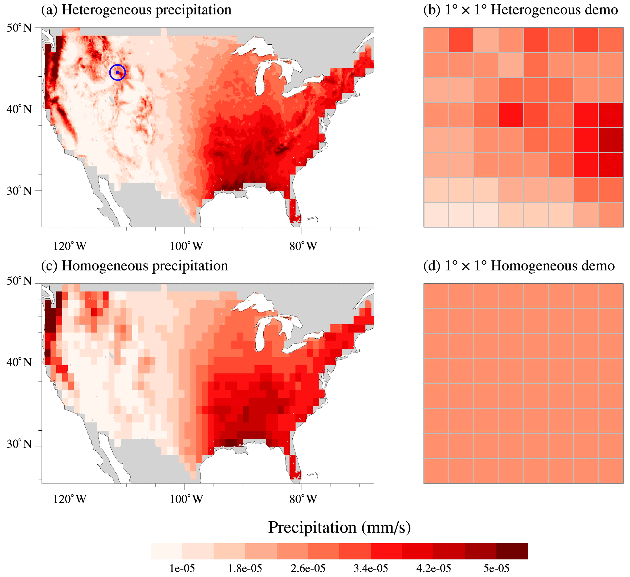
Figure 1 Annual climatology of (a) heterogeneous and (c) homogeneous precipitation over CONUS. The corresponding (b) heterogeneous and (d) homogeneous precipitation over a 1^∘ × 1^∘ region (latitude: 37–38^∘ N, longitude: 111–110^∘ W, the blue marker in a) is also shown.

2.2.2 Heterogeneous and homogeneous inputs

We prepared heterogeneous and homogeneous inputs at 0.125^∘ × 0.125^∘. The difference between the two datasets is whether the input values within each 1^∘ × 1^∘ region of ELM are spatially heterogeneous or homogeneous. The SOIL, TOPO, and LULC were first mapped from their original resolutions to 0.125^∘ × 0.125^∘ resolution, using the Earth System Modeling Framework (ESMF) regridding tool. Specifically, the first-order conservative interpolation was used for upscaling the dataset (e.g., soil texture), while the nearest neighbor interpolation was used for downscaling the dataset (e.g., soil color). These 0.125^∘ resolution datasets are used as the heterogeneous inputs (Fig. 1a and b). Then, for each dataset, we replaced the heterogeneous values of the 64 0.125^∘ × 0.125^∘ grids within each 1^∘ × 1^∘ region by the mean of the 64 grids (see Fig. 1b vs. Fig. 1d). The temporally varying datasets (e.g., hourly ATM and monthly climatology LAI) were processed at each time interval. As an example, Fig. 1 compares the annual climatology of the heterogeneous and homogeneous precipitation.

2.3 Experimental design and analysis

We conducted two sets of ELM experiments over CONUS. The first set contains 16 experiments with different combinations of heterogeneous and homogeneous inputs from the four heterogeneity sources (Table 2). These experiments were used to quantify the influence of different heterogeneity sources on the ELM simulations. The second set of 13 experiments was further conducted to analyze the impact of heterogeneity from individual components of three heterogeneity sources (Table 3). As LULC has no explicit individual component, we only analyzed the components of ATM with seven experiments, SOIL with three experiments, and TOPO with three experiments. Each experiment only contains one heterogeneous input while other components are homogeneous. Both the first and second set of experiments were configured at 0.125^∘ × 0.125^∘ spatial resolution. The 40-year NLDAS-2 forcing from 1980–2019 was cycled twice to drive the ELM run for 80 years. The first 50-year run was used as model spin-up and the last 30-year simulation (corresponding to atmospheric forcing from 1990–2019) was used for further analysis.

Table 2 The first set of 16 experiments with inputs from ATM, SOIL, LULC, and TOPO (0 and 1 denote homogeneous and heterogeneous input from the four heterogeneity sources, respectively).

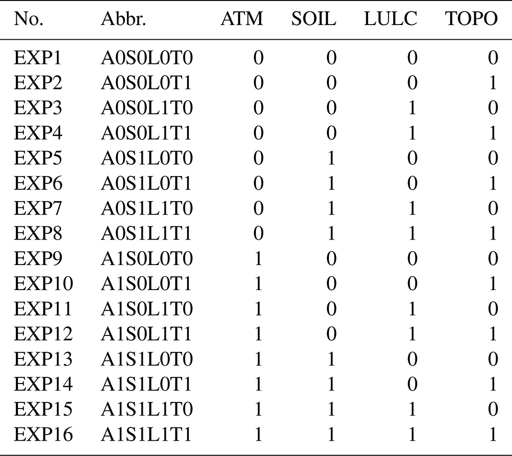
Table 3 The second set of 13 experiments with inputs from each component of the heterogeneity sources.

Our analysis focused on water partitioning, energy partitioning, and related flux variables. The water partitioning is quantified as the ratio between evapotranspiration (ET) and precipitation (P), i.e., $\text{ET}/P$, and the ratio between runoff (R) and precipitation (P), i.e., $R/P$. The energy partitioning is quantified using the evaporative fraction (EF), which equals the ratio between latent heat (LH) and the sum of latent heat and sensible heat (SH), i.e., $\text{EF}=\frac{\text{LH}}{\text{LH}+\text{SH}}\cdot \mathrm{100}\left(\mathit{\%}\right)$. First, the 30-year monthly, seasonal, and annual climatological means were calculated for each experiment at 0.125^∘ × 0.125^∘ resolution for the five variables of interest (i.e., P, ET, R, LH, and SH). Second, the water and energy partitioning variables (i.e., $\text{ET}/P$, $R/P$, EF) were computed at 0.125^∘ × 0.125^∘ resolution. Third, the standard deviations (SDs) of these variables' climatological mean were calculated for each 1^∘ × 1^∘ region from its embedded 64 0.125^∘ × 0.125^∘ grids. These 1^∘ × 1^∘ resolution SDs of the first and second set of experiments were used in the following analysis.

For the first set of 16 experiments, we utilized the Sobol' sensitivity analysis to quantify the relative importance of the four heterogeneity sources on water and energy simulations. The detail of the Sobol' sensitivity analysis is described in Sect. 2.4.

The Sobol' method was not used for the second set of 13 experiments because a comprehensive Sobol' analysis needs 2¹³ experiments, which is computationally infeasible. Instead, the calculated SD of each experiment is used to quantify the impact of heterogeneity of each component, as each experiment only contains one heterogeneous input. Therefore, we compared the SDs between each experiment to determine the relative importance of each component with heterogeneous input (without considering interactions between different components).

2.4 The Sobol' sensitivity indices

The Sobol' sensitivity analysis (Sobol', 1993) was applied to quantify the sensitivity of spatial variation (i.e., SD) of water and energy partitioning to the four heterogeneity sources based on the first set of 16 experiments. Here, the Sobol' first-order sensitivity index measures the direct contribution of a single heterogeneity source to the target variable's spatial variability (e.g., EF's SD). Sobol' higher-order (i.e., second or higher order) sensitivity indices quantify the contribution by the interactions between a given heterogeneity source with other heterogeneity sources. The sum of all higher-order indices quantifies the overall interaction effects. Sobol' total sensitivity index measures the total contribution of a given heterogeneity source, which considers both the first-order and the interaction effects (Zhang et al., 2015; Saltelli et al., 2010). Specifically, the Sobol' total sensitivity index (${\text{ST}}_{X_i}$) and the first-order sensitivity index ($S_{X_i}$) are given as (Saltelli et al., 2010)

$$\begin{array}{}\text{(1)}& {\displaystyle }& {\displaystyle }{\text{ST}}_{X_i}={\displaystyle \frac{E_{X_{\sim i}}\left(V_{X_i}\left(Y\mathrm{|}{X}_{\sim i}\right)\right)}{V\left(Y\right)}}\text{(2)}& {\displaystyle }& {\displaystyle }{S}_{X_i}={\displaystyle \frac{V_{X_i}\left(E_{X_{\sim i}}\left(Y\mathrm{|}{X}_i\right)\right)}{V\left(Y\right)}},\end{array}$$

where X_i is the ith heterogeneity source (e.g., ATM, SOIL, LULC, and TOPO), X_∼i denotes the other heterogeneity sources except X_i, Y is the SD of a given simulated variable for a given experiment, and V(Y) is the total variance of the given variable's SDs across all 16 experiments.

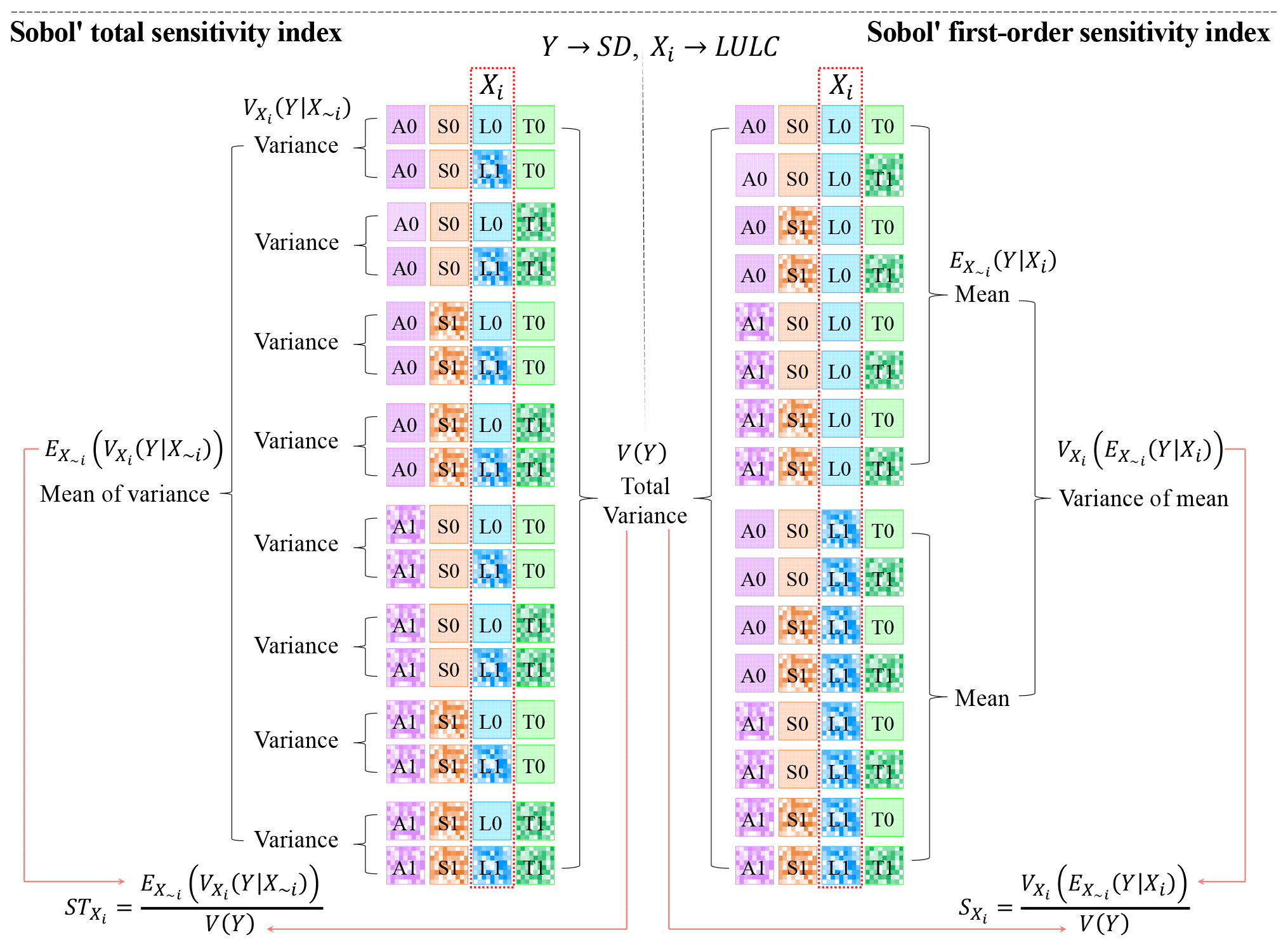
Figure 2 Schematic flowchart for the calculation of Sobol' total and first-order indices for LULC (i.e., X_i=LULC). The notation (e.g., A0, S0, L0, T0) in each box corresponds to the experiment abbreviation listed in Table 2. A box with (without) mosaic represents heterogeneous (homogeneous) input. The Sobol' total sensitivity index is computed by dividing the 16 experiments into eight subgroups, such that in each subgroup, ATM, SOIL, and TOP are fixed, except for LULC. The Sobol' first-order sensitivity index is computed by dividing the 16 experiments into two subgroups, such that in each subgroup, LULC is fixed.

Figure 2 illustrates the calculation of Sobol' total and first-order sensitivity indices for LULC (i.e., X_i=LULC) as follows:

1. For the calculation of ${\text{ST}}_{X_i}$, first, following Zheng et al. (2019), the SDs of the 16 experiments are reformed into eight subgroups based on experiments with different combinations of X_∼i. Second, the variance of SD for each subgroup is computed. Third, the mean of SD variances across 8 subgroups is computed. Fourth, ${\text{ST}}_{X_i}$ is calculated using Eq. (1).

2. For the calculation of $S_{X_i}$, first, the SDs of the 16 experiments are reformed into two subgroups based on the experiments either with heterogeneous or homogeneous X_i. Second, the mean of SDs for each subgroup is computed. Third, the variance of mean SD across two subgroups is calculated. Fourth, $S_{X_i}$ is computed using Eq. (2).

The Sobol' sensitivity indices for ATM, TOPO, and SOIL can be computed similarly.

The interaction effect index, ${\text{SI}}_{X_i}$, can be computed as

$$\begin{array}{}\text{(3)}& {\text{SI}}_{X_i}={\text{ST}}_{X_i}-S_{X_i}.\end{array}$$

The corresponding fraction of first-order index ($f_{S_{X_i}}$) and interaction effect index ($f_{{\text{SI}}_{X_i}}$) contributing to the total sensitivity index for X_i can be given as

$$\begin{array}{}\text{(4)}& {\displaystyle }& {\displaystyle }{f}_{S_{X_i}}={\displaystyle \frac{S_{X_i}}{{\text{ST}}_{X_i}}}\times \mathrm{100}\text{(5)}& {\displaystyle }& {\displaystyle }{f}_{{\text{SI}}_{X_i}}=\mathrm{100}-f_{S_{X_i}}.\end{array}$$

A more detailed demonstration for the calculation of Sobol' total sensitivity index, first-order sensitivity index, and the interaction effect index is presented in Appendix A. In this paper, the Sobol' total sensitivity index is mainly contributed by Sobol' first-order sensitivity index (see details in Sect. 3.1). Therefore, to make this paper concise, our analysis is based chiefly on Sobol' total sensitivity index if not explicitly pointed out otherwise.

2.5 ERA5-Land reanalysis dataset

We further compared the first set of experiments with ERA5-Land reanalysis (the land component of the fifth generation of European Centre of Medium-range Weather Forecast reanalysis) (Muñoz-Sabater et al., 2021) to demonstrate the added value in ELM simulations with consideration of heterogeneity sources. ERA5-Land provides a consistent view of terrestrial water and energy cycles at high spatial and temporal resolutions. The monthly ERA5-Land data at 0.1^∘ × 0.1^∘ resolution were used in this study. First, the monthly data were regridded using the ESMF regridding tool via the first-order conservative interpolation to 0.125^∘ × 0.125^∘ resolution, which is consistent with the resolution of our sensitivity experiments. Second, the annual and seasonal climatological means for related variables (e.g., ET, R, SH) were computed. Third, SD for each variable was calculated within each 1^∘ × 1^∘ region for further comparisons with the ELM simulations.

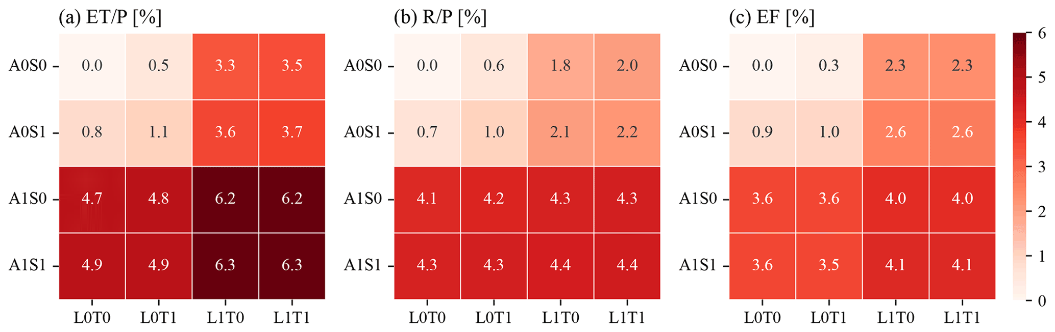
Figure 3 CONUS-averaged SD of the annual climatology of (a) $\text{ET}/P$, (b) $R/P$, and (c) EF. Combining the x axis label for LULC and TOPO and the y axis label for ATM and SOIL indicates the names of the experiments listed in Table 2, highlighting the use of heterogeneous (1) and homogeneous (0) inputs for each heterogeneity source.

3 Results

3.1 CONUS overall heterogeneity sensitivities

The inclusion of more heterogeneity sources leads to larger spatial variability in the simulated $\text{ET}/P$, $R/P$ and EF (Fig. 3). For example, comparing experiment A0S0L0T0 with A1S0L0T0 that includes the ATM heterogeneity, the CONUS-averaged SD for $\text{ET}/P$ increases from 0 % to 4.7 % (Fig. 3a). By further comparing experiments in the first and third rows with the second and fourth rows, ATM always increases the spatial variability of water and energy partitioning. Similarly, LULC heterogeneity also shows large impacts on the spatial variability for the partitioning variables, as indicated by comparing experiments in the first and third columns with the second and fourth columns. However, heterogeneity in SOIL and TOPO show negligible impact. The effects of the heterogeneity sources on the spatial variability of water and energy partitioning are mainly located in western and central CONUS (Fig. S1 in the Supplement), which is consistent with the spatial variability of the heterogeneity inputs for variables such as precipitation, air temperature, and longwave radiation (Fig. S2 in the Supplement).

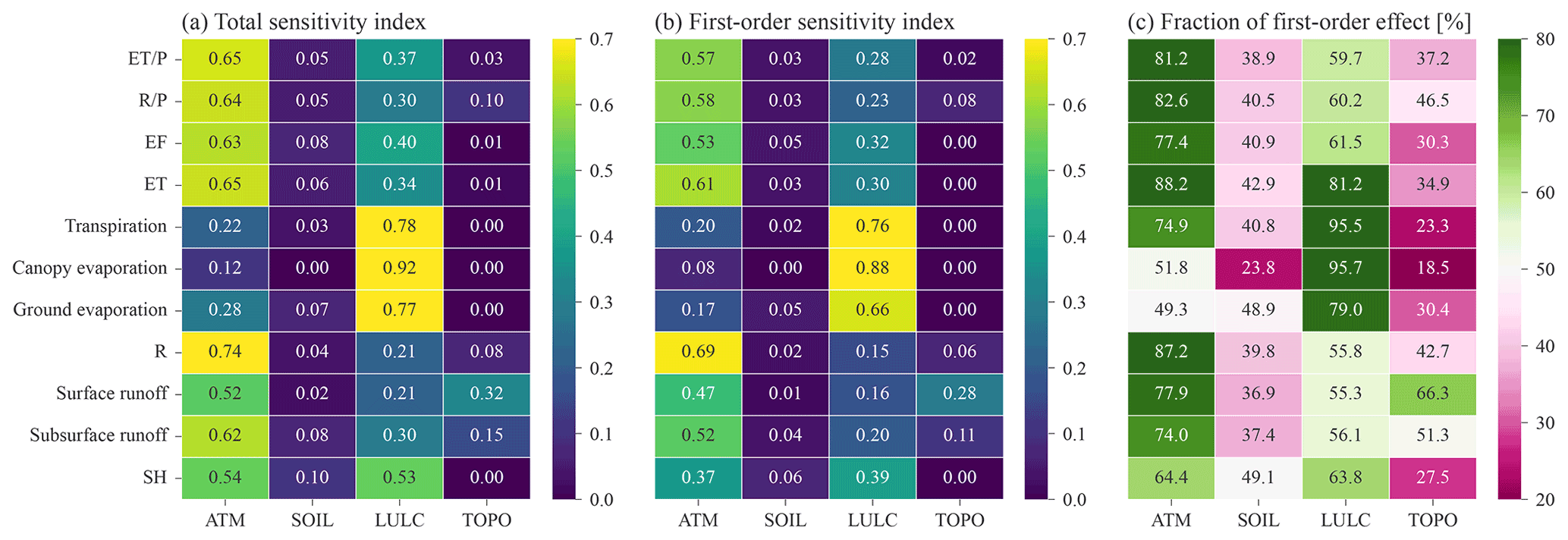
Figure 4 CONUS-averaged (a) Sobol' total sensitivity index, (b) Sobol' first-order sensitivity index, and (c) the fraction of first-order effect for the sensitivity of spatial variability of different variables (rows) to the four heterogeneity sources (columns).

ATM, with the largest Sobol' total sensitivity index, is the most important heterogeneity source to determine the spatial variability of water and energy partitioning ($\text{ET}/P$, $R/P$, EF in Fig. 4a). LULC is the second most important heterogeneity source (Fig. 4a). Even though ATM dominates the spatial heterogeneity of total ET, LULC is the main contributor to the spatial variability of the ET components of transpiration, canopy evaporation, and ground evaporation. The first-order sensitivity indices show similar patterns as the total sensitivity indices (Fig. 4b vs. Fig. 4a). For the ATM and LULC, their first-order sensitivity indices contribute more than 60 % of the total sensitivity indices in determining the spatial variability of water and energy partitioning ($\text{ET}/P$, $R/P$, EF in Fig. 4c). Therefore, the total heterogeneity effects of ATM or LULC are mainly due to their own heterogeneity rather than their interactions with other heterogeneity sources. The small proportion of the rest of the total heterogeneity effects of ATM and LULC is contributed by their interactions with other heterogeneity sources (Fig. S3b in the Supplement).

The heterogeneity of SOIL and TOPO marginally contributes to the spatial variability of water and energy partitioning (Fig. 4a). Their effects contributed from their own heterogeneity and their interactions with other heterogeneity sources are relatively small (Figs. 4b and S3a in the Supplement). TOPO shows larger impacts on the spatial variabilities of the runoff components than the total runoff (Fig. 4a). TOPO's impact on the total runoff is mainly due to its interaction effects with other heterogeneity sources, but its impacts on surface and subsurface runoff are primarily contributed by its own heterogeneity (Fig. 4c).

Generally, high values of total sensitivity indices are mostly contributed by the first-order sensitivity index (Figs. 4a, b and S5 in the Supplement). Since our main goal is to analyze the major heterogeneity sources with a large Sobol' total sensitivity index, the results presented in the subsequent sections are based chiefly on Sobol' total sensitivity index.

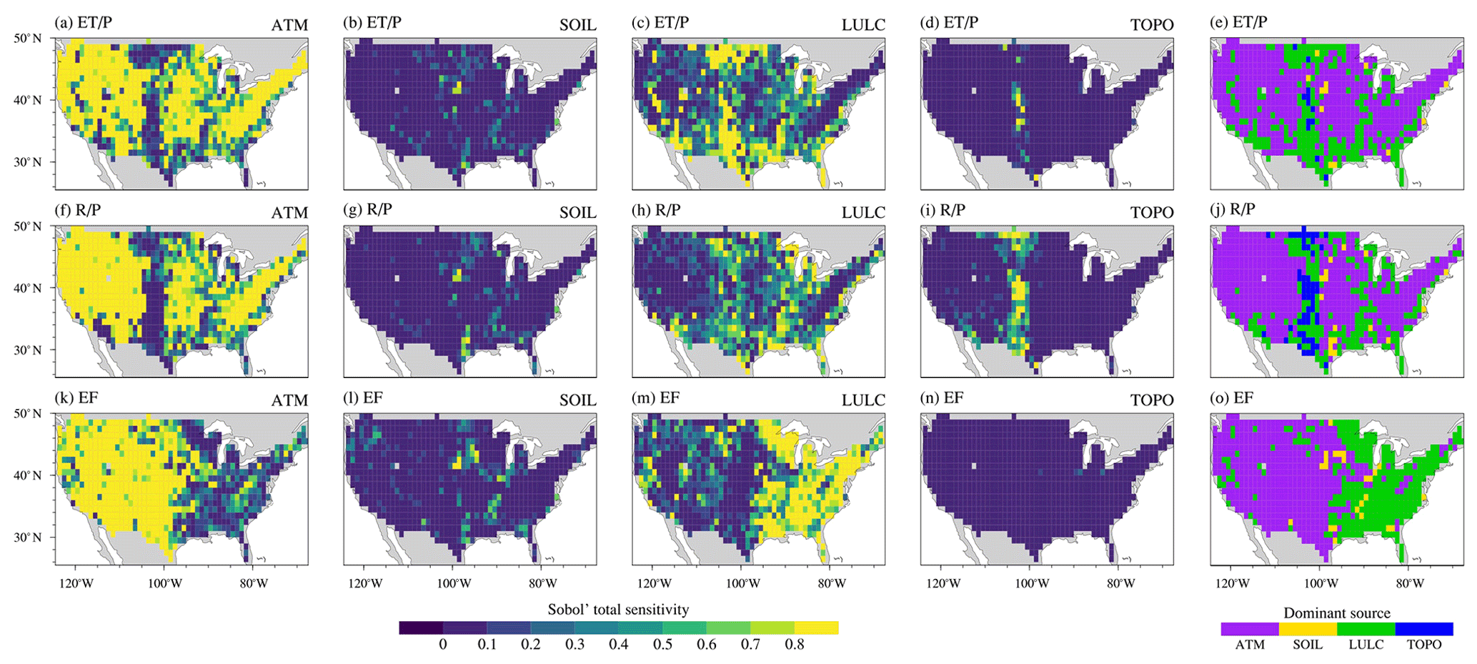
Figure 5 Spatial patterns of Sobol' total sensitivity index for the four heterogeneity sources (column one–four) and the corresponding dominant sources (column five) for the spatial variability of water ($\text{ET}/P$ and $R/P$) and energy (EF) partitioning.

3.2 Spatial patterns of heterogeneity sensitivities

The sensitivity of the four heterogeneity sources shows different spatial patterns over CONUS (Fig. 5). The water partitioning components, $\text{ET}/P$ and $R/P$, exhibit similar spatial patterns of Sobol' sensitivity index for any given heterogeneity source (Figs. 5a–d and 4f–i). ATM shows high Sobol' sensitivity index over most CONUS regions for water and energy partitioning. It dominates the spatial variability of $\text{ET}/P$ and $R/P$ over eastern and western CONUS but not central CONUS (Fig. 5e and j). For the spatial variability of EF, ATM mostly shows dominant effects over central and western CONUS (Fig. 5o). LULC is the second most dominant heterogeneity source and dominates most regions over eastern CONUS, although LULC also dominates smaller regions for the spatial variability of $\text{ET}/P$ and $R/P$ over central and southeastern CONUS (Fig. 5e and j). Overall, ATM Sobol' total sensitivity index has opposite spatial patterns compared to LULC Sobol' total sensitivity index (Fig. B1 in Appendix B). Therefore, ATM and LULC show complementary contributions to the spatial variability of water and energy partitioning across CONUS. Although TOPO overall has low Sobol' index, it dominates the spatial variability of $R/P$ over central CONUS (Fig. 5j). SOIL has negligible impacts over most regions of CONUS for the spatial variability of both water and energy partitioning. The spatial distributions of Sobol' first-order sensitivity indices for the four heterogeneity sources are similar to the Sobol' total sensitivity indices (Fig. 5 vs. Fig. S4 in the Supplement). First-order sensitivity indices contribute dominantly to the total sensitivity indices (Fig. S5). Therefore, most of the heterogeneity effects on water and energy partitioning by each heterogeneity source come from its own heterogeneity with small proportions from its interaction effects with other heterogeneity sources.

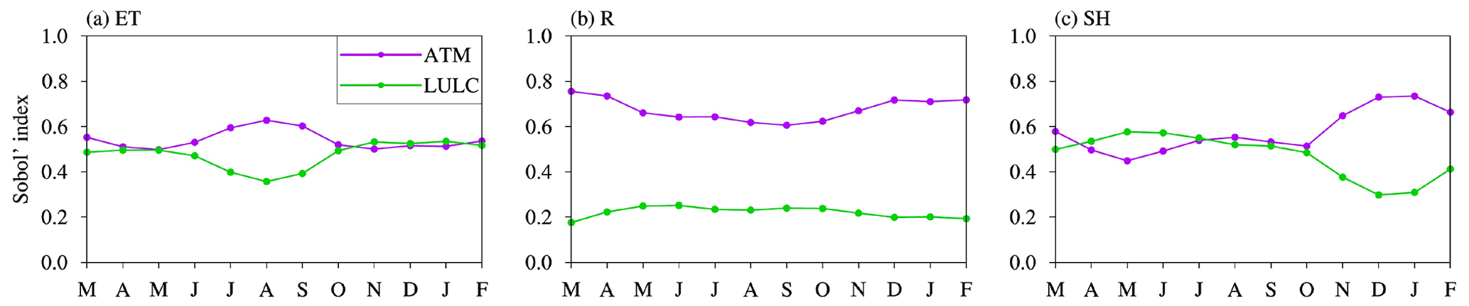
Figure 6 Monthly variations of CONUS-averaged ATM and LULC Sobol' index for (a) ET, (b) R, and (c) SH.

3.3 Seasonal variation of heterogeneity sensitivities

The impacts of ATM and LULC on the spatial variability of water and energy fluxes show more seasonal variations than the impacts of SOIL and TOPO (Fig. 6, SOIL and TOPO are not shown here). This is because ATM and LULC consist of time-varying inputs to the ELM simulations, but SOIL and TOPO are time-invariant inputs. Even though the spatial distribution of LULC is temporally static, the monthly variations in LAI and SAI of different land cover types could affect the seasonal variation of sensitivity. The heterogeneity impacts of ATM and LULC on the spatial variability of water and energy fluxes show complementary seasonal variations. The effect of ATM on the ET spatial variability is larger in July–September than in other months (Fig. 6a), while LULC shows smaller Sobol' index in July–September. The sensitivity of transpiration and canopy evaporation shows the same seasonal variations (Fig. C1d–f in Appendix C). The spatial variability of R is more sensitive to ATM in the cold season (December–April, Fig. 6b), especially for its component of surface runoff (Fig. C1g). The sensitivity of SH spatial variability to ATM is larger in the non-growing season (i.e., November–March) than in the growing season (i.e., April–October), with the LULC Sobol' index showing opposite seasonal variations (Fig. 6c).

The spatial patterns of dominant regions by the four heterogeneity sources vary over different seasons. Compared with spring and winter, ATM dominates the ET spatial variability in more regions than in summer and fall when ATM is more dominant over eastern CONUS (Table 4 and Fig. S6a–d in the Supplement). LULC shows opposite seasonal spatial patterns with more dominant regions in eastern CONUS over spring and winter. As for the R spatial variability, TOPO shows large spatial variation of its dominant regions over different seasons (Fig. S6f–i). Besides its dominant contribution in central CONUS over all seasons, TOPO also dominates the R spatial variability in parts of eastern US in the summer and autumn (Fig. S6g and h). For the SH spatial variability, ATM has more contributions in the fall and winter but smaller contributions in spring and summer than LULC (Table 4). LULC shows more dominant regions over eastern CONUS, especially in spring and summer (Fig. S6k and l). To understand the seasonal variations of dominant heterogeneity sources, the seasonal variations of Sobol' total sensitivity index and induced R's SD are demonstrated at one grid cell over eastern US (Fig. S7 in the Supplement). Compared with other heterogeneity sources, ATM-induced R's SD shows an apparent seasonal variation with high values in spring and winter but small values in summer and fall (Fig. S7b). Therefore, ATM is the dominant heterogeneity source in spring and winter. Even though TOPO- and SOIL-induced R's SDs show slight seasonal variations (Fig. S7), they dominate R's spatial variability in summer and fall, respectively.

Table 4 Grid percentage of the dominant heterogeneity source in determining the spatial variability of ET, R, and SH for four seasons and annual mean (ANN).

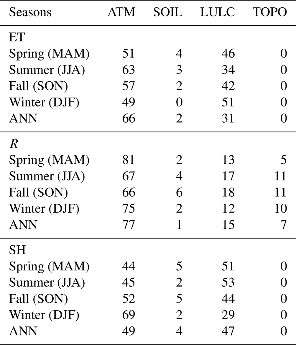
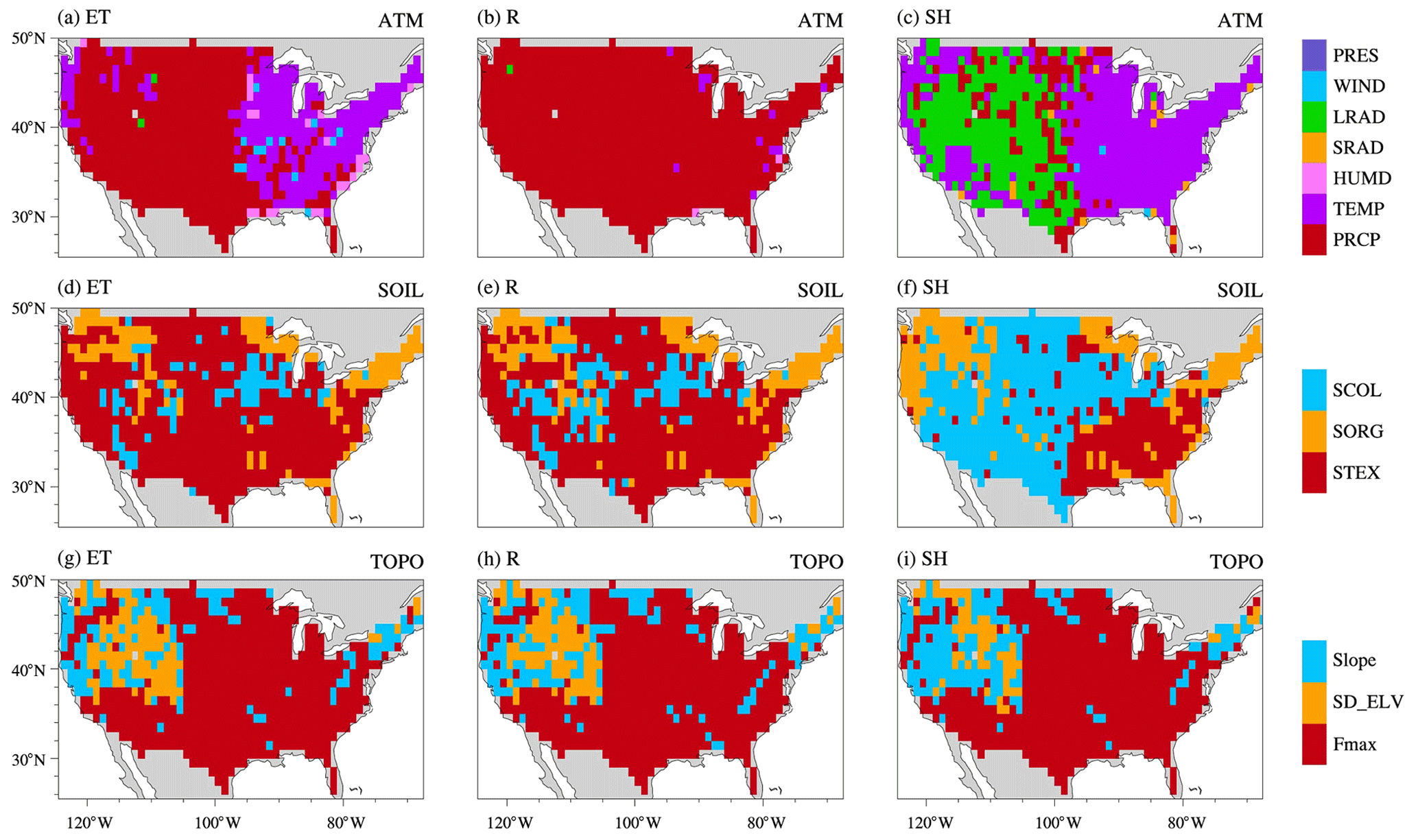
Figure 7 The largest induced spatial variability for the annual climatological mean of ET (a, d, g), R (b, e, h), and SH (c, f, i) induced by each component of ATM (a–c), SOIL (d–f), and TOPO (g–i).

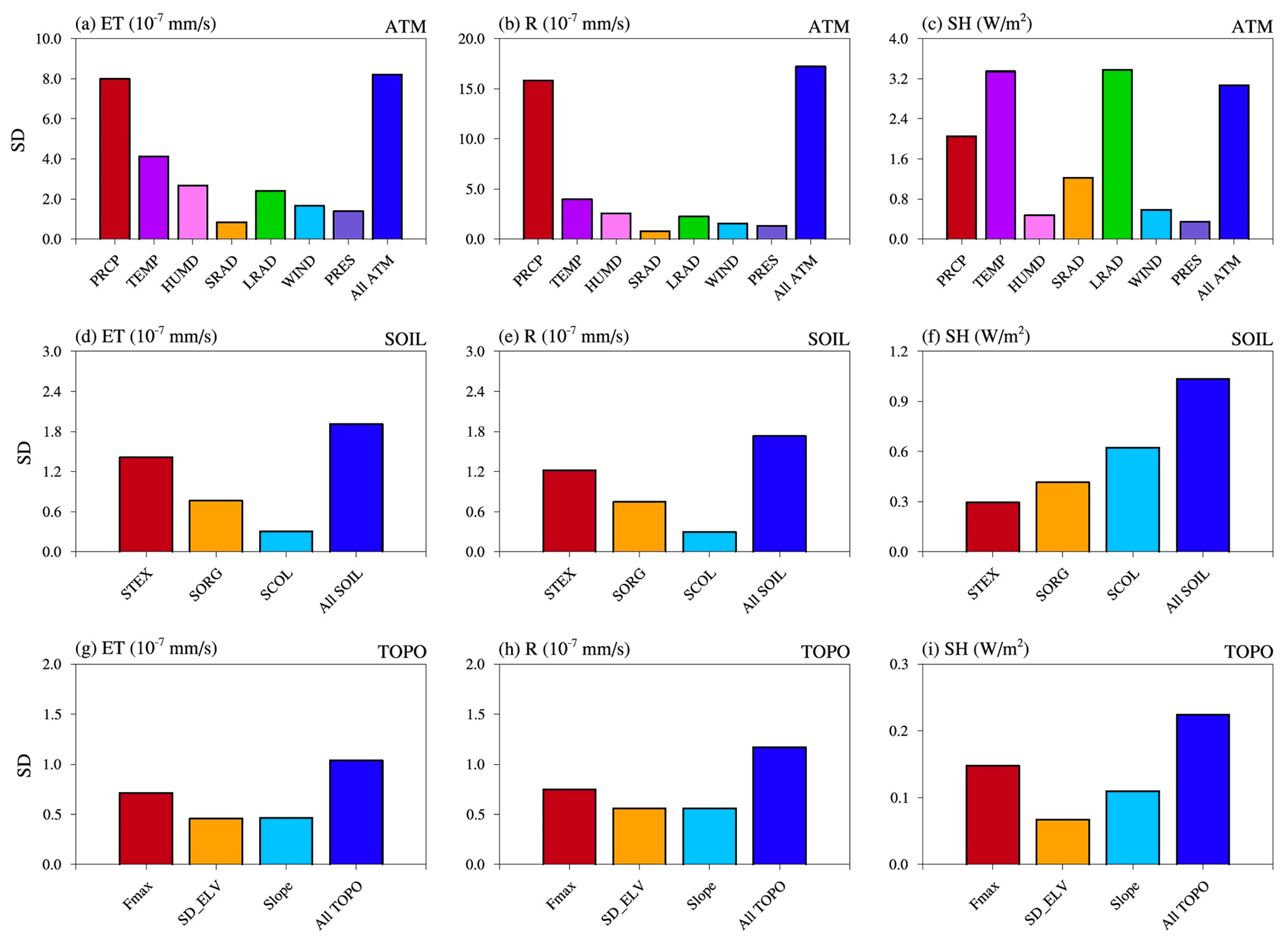
Figure 8 CONUS-averaged spatial variability for the annual climatological mean of ET (a, d, g), R (b, e, h), and SH (c, f, i) by each component and all components of ATM (a–c), SOIL (d–f), and TOPO (g–i).

3.4 Effects of heterogeneity components

Based on the second set of 13 experiments, we analyzed the heterogeneity effects by each component of ATM, SOIL, and TOPO (Fig. 7), respectively. Precipitation is the largest ATM heterogeneity source in determining the spatial variability of water fluxes (Fig. 7a and b), especially over western and central CONUS for ET (Fig. 7a) and almost the entire CONUS for R (Fig. 7b). Air temperature dominates the spatial variability of ET in eastern CONUS (Fig. 7a). The spatial variability of SH is mainly dominated by the incoming longwave radiation in western CONUS and by the air temperature in eastern CONUS (Fig. 7c). Longwave radiation provides more energy input and contributes more to the SH spatial variability than shortwave radiation (Fig. 8c). Among the SOIL components, soil texture, which can influence soil moisture and runoff generation, shows the largest effects on the ET and R spatial variability over most CONUS regions (Figs. 7d, e and 8d, e). Soil color, affecting the surface albedo and energy balance, shows the largest impacts on the SH spatial variability over central CONUS (Figs. 7f and 8f). Fmax is the most essential TOPO component, offering the largest effects on the spatial variability of ET, R, and SH over most CONUS regions (Figs. 7g–i and 8g–i). Fmax regulates surface runoff generation and infiltration, and therefore influences the soil moisture, ET, and SH. SD_ELV and slope can affect surface water and snow cover fraction, and consequently, they show the largest impacts over northwestern CONUS regions with mountains and snowpack.

The spatial variability induced by all components (of ATM, SOIL, or TOPO) is larger than that induced by each individual component. However, it is smaller than the sum of the spatial variability induced by each component (Fig. 8). For example, the CONUS-averaged SD for ET caused by all SOIL components is 1.9 (10⁻⁷ mm s⁻¹), which is smaller than 2.5 (10⁻⁷ mm s⁻¹), the sum of the SD of ET induced by STEX, SORG, and SCOL (Fig. 8d). Therefore, the additional SD induced by an additional heterogeneity component decreases, suggesting that the effect of heterogeneity on the spatial variability of water and energy fluxes saturates due to the interaction effects between heterogeneity components on related water and energy processes.

Figure 9 CONUS-averaged absolute difference of SD between 16 ELM experiments and ERA5-Land reanalysis for the annual (first column) and seasonal (second–fifth column) climatological mean of ET (a, d, g, j, m), R (b, e, h, k, n), and SH (c, f, i, l, o).

3.5 Comparison with ERA5-Land reanalysis

Higher consistency of the spatial variability between the simulations and ERA5-Land reanalysis (i.e., smaller SD difference) is obtained when more sources of heterogeneity are accounted for in the simulations for ET, R, and SH (Fig. 9). ATM and LULC dominate the improvements in the spatial variability of model simulations. Generally, ATM heterogeneity leads to more or similar improvements than LULC heterogeneity for ET, R, and SH over all seasons. For example, in Fig. 9a, ATM induced larger improvements, as shown by comparing experiments in the first and third rows with the second and fourth rows, than the LULC-induced improvements, comparing experiments in the first and third columns with the second and fourth columns. The SD difference is usually larger over MAM and JJA than SON and DJF, probably due to the heterogeneity difference between the NLDAS and ERA5 atmosphere forcing as ATM is the major heterogeneity contributor.

Improvements of the spatial variability of model simulations are primarily distributed over western and eastern CONUS for ET, R, and SH (e.g., Figs. S8 and S9 in the Supplement first column vs. fourth column). Overall, the ELM simulated ET and SH have smaller SDs than those of ERA5_Land (Fig. S9d and l). Meanwhile, the simulated R has larger SD especially in the western US than that of ERA5_Land, probably mainly due to ATM's heterogeneity effects (Fig. S9e vs. Fig. S9g). For ET and R, ATM mainly increases their spatial variability over western and eastern CONUS (Fig. S8a vs. Fig. S8c and Fig. S8e vs. Fig. S8g) and LULC mostly shows changes over eastern CONUS (Fig. S8a vs. Fig. S8b and S8e vs. Fig. S8f). Both ATM and LULC increase SH spatial variability over western and eastern CONUS (Fig. S8i vs. Fig. S8j and Fig. S8i vs. Fig. S8k).

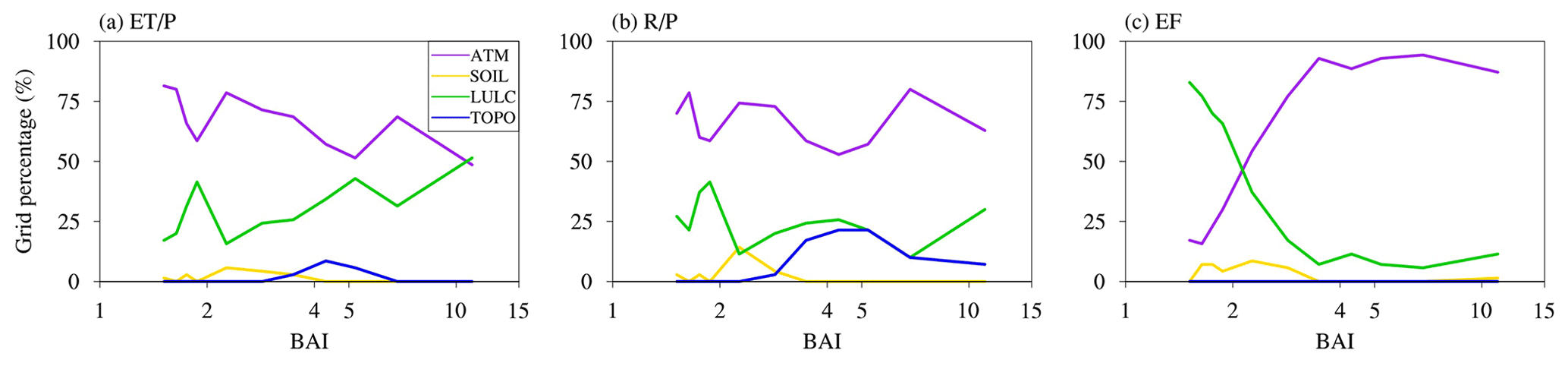
Figure 10 The grid percentage of dominant heterogeneity sources along with Budyko's aridity index. A higher aridity index means more arid.

4 Discussions

ATM and LULC are the two most essential heterogeneity sources contributing to the spatial variability of water and energy partitioning. Their total heterogeneity effects are mostly contributed by their own heterogeneity, with small proportions contributed by their interactions with other heterogeneity sources. Simon et al. (2021) also found that the heterogeneous meteorological forcing is the primary driver for the spatial variability of latent heat and sensible heat in WRF simulations. The Sobol' sensitivity index averaged over the same region (a 100 km × 100 km domain centered at 36.6^∘ N, 97.5^∘ W) as Simon et al. (2021) also indicates that ATM is the dominant heterogeneity source. Therefore, better representation of ATM heterogeneity in climate models is crucial for modeling the water and energy partitioning, especially for the three major components of precipitation, air temperature, and longwave radiation. Tesfa et al. (2020) compared several simple approaches to capturing ATM heterogeneity for downscaling the grid mean precipitation to topography-based subgrids for land surface modeling. Besides ATM, LULC is the second most crucial heterogeneity source. Notably, anthropogenic land use and land cover change has been shown to have large impacts on land–atmosphere interaction, land surface hydrology, and associated extreme events (Findell et al., 2017; Li et al., 2018, 2015; Swann et al., 2010; Zeng et al., 2017; Yuan et al., 2021; Pielke et al., 2007). Therefore, the heterogeneity of LULC should also be well considered in climate modeling.

ATM and LULC show complementary contributions to the spatial variability of water and energy partitioning spatially over CONUS and temporally in different seasons. Sobol' sensitivity analysis is a standardized quantification of the relative importance of different heterogeneity sources. The sum of the Sobol' indices for the four heterogeneity sources roughly equals one. As the two dominant heterogeneity sources, ATM Sobol index and LULC Sobol' index dominate the sum of all Sobol' indices. Hence, they show complementary patterns spatially (Fig. B1) and temporally (Fig. 6). In addition, ATM and LULC show complementary contributions across different climate zones. Budyko's aridity index (BAI, Budyko, 1974), which is the ratio of annual net radiation to the product of the latent heat of water vaporization and the annual precipitation, was calculated using the outputs from EXP16. From humid (low BAI) to arid climate (high BAI), a decreasing fraction of the CONUS region is dominated by ATM in determining the $\text{ET}/P$ spatial variability (Fig. 10a). At the same time, LULC shows an increasing contribution to the $\text{ET}/P$ spatial variability with BAI. The spatial variability of energy partitioning exhibits even more complementarity between the ATM and LULC contributions from arid regions to humid regions (Fig. 10c). In more arid regions limited by water, EF spatial variability is much more dominated by heterogeneity of ATM, likely through the heterogeneous precipitation, but in humid regions limited by energy, LULC dominates the EF spatial variability through its influence on surface albedo and surface roughness.

SOIL and TOPO show relatively small impacts on the spatial variability of water and energy partitioning. However, TOPO has a dominant influence on the $R/P$ spatial variability over the transitional zone (Fig. 10b) of central CONUS located between the arid western CONUS and the humid eastern CONUS (Fig. 5). TOPO's impact on the total runoff is mainly due to its interaction effects with other heterogeneity sources (Fig. 4). SOIL shows some dominant effects on the spatial variability of water and energy partitioning over a small proportion of humid regions (Fig. 10). The heterogeneity in SOIL and TOPO was derived from coarse resolution data at 0.125^∘ × 0.125^∘ spatial resolution, which could be a possible reason for the minor SOIL and TOPO effects. Singh et al. (2015) found that CLM4.0 did not show much improvement when model resolution increased from ∼ 100 km to ∼ 25 km, but improvement was noticeable at finer 1 km resolution. Additionally, exclusion of lateral subsurface flow in ELMv1 could also lead to underestimation of the contributions from SOIL and TOPO.

The current study excluded a few land surface processes that have been included in LSMs in the last decade, limiting our ability to assess the role of land surface heterogeneity in spatiotemporal variability of energy and water partitioning. For example, the hillslope processes of lateral ridge-valley flow and the insolation contrasts between sunny and shady slopes are crucial for land surface modeling (Fan et al., 2019; Taylor et al., 2012; Clark et al., 2015; Scheidegger et al., 2021), but they are neglected in this study. Swenson et al. (2019) incorporated the representative hillslope concept into the CLM5 and they found that subgrid hillslope process induced large differences in evapotranspiration between upland and lowland hillslope columns in arid and semiarid regions. Krakauer et al. (2014) suggested that the magnitude of between-grid groundwater flow becomes significant over larger regions at higher model resolution. Xie et al. (2020) also demonstrated the importance of groundwater lateral flow in offsetting depression cones caused by intensive groundwater pumping. Fang et al. (2017) compared the ACME Land Model (the earlier version of ELM) and the three-dimensional ParFlow variably saturated flow model (Maxwell et al., 2015), underscoring the ELM limitation in capturing topography's influence on groundwater and runoff. Additionally, topography also significantly influences insolation, including the shadow effects and multi-scattering between adjacent terrain. Hao et al. (2021) implemented a sub-grid topographic parameterization in ELM, which improves the simulated surface energy balance, snow cover, and surface air temperature over the Tibetan Plateau. The inclusion of plant hydraulics has also shown essential improvements in water and carbon simulations under drought conditions (Li et al., 2021; Fang et al., 2021), which should also be considered in future research, especially as vegetation may experience more hydroclimate drought stress in projected future climate conditions (Yuan et al., 2019; Xu et al., 2019; Li et al., 2020). The subgrid downscaling of atmospheric forcing (Tesfa et al., 2020), which could further enhance the representation of heterogeneity effects on water and energy simulations, is also unaccounted for in this study.

5 Conclusions

This study comprehensively investigated the impacts of different heterogeneity sources (i.e., ATM, LULC, SOIL, TOPO) on the spatial variability of water and energy partitioning over CONUS. Two sets of experiments were conducted based on different combinations of spatially heterogeneous and homogeneous datasets. Based on the first set of 16 experiments, Sobol' total and first-order sensitivity indices were utilized to identify the relative importance of the four heterogeneity sources. The second set of 13 experiments were further used to assess the influence from individual components of ATM, SOIL, and TOPO. Our results show that ATM and LULC are the two dominant heterogeneity sources in determining the spatial variability of water and energy partitioning, largely contributed by ATM's or LULC's own heterogeneity and slightly contributed by their interactions with other heterogeneity sources. Their heterogeneity effects are spatially complementary across CONUS and temporally complementary across seasons. The complementary contributions of ATM and LULC reflect the overall negligible impacts of SOIL and TOPO, but the complementarity also reflects physically the clear demarcation of climatic zones across CONUS, featuring the arid, water-limited western CONUS dominantly influenced by ATM (precipitation, in particular) and the humid, energy-limited eastern CONUS dominantly influenced by LULC. In the transitional climate zone of central CONUS, TOPO shows some dominant influence on the $R/P$ spatial variability. The overall most essential components for ATM (precipitation, temperature, and longwave radiation), SOIL (soil texture and soil color), and TOPO (Fmax) were also identified. Comparison with ERA5-Land reanalysis reveals that accounting for more sources of heterogeneity improved the simulated spatial variability of water and energy fluxes, although such improvements tend to saturate as more heterogeneous sources were added.

The relative importance of different heterogeneity sources quantified in this study is useful for prioritizing spatial heterogeneity to be included for improving land surface modeling. We note, however, that the present assessment is limited by how well the input datasets capture the spatiotemporal heterogeneity and how well the land surface model represents processes such as hillslope hydrology and topographic effect on solar radiation that are influenced by land surface heterogeneity. This motivates the use of more process-rich models such as distributed or three-dimensional subsurface hydrology models to provide benchmarks of the relative importance of heterogeneity sources to help prioritize the future development of land surface models to improve modeling of energy and water fluxes.

Appendix A: Demonstration of Sobol' index calculation

Here, we give an example for the calculation of Sobol' total, first-order, and interaction effect indices, ST_LULC, S_LULC, and SI_LULC to quantify the sensitivity of EF's spatial variability to LULC in a 1^∘ × 1^∘ region at 39.5^∘ N and 107.5^∘ W.

1. Calculation of ST_LULC (Table A1). Following Zheng et al. (2019) and based on Eq. (1) and Fig. 2, the 16 experiments are grouped into eight subgroups containing two experiments, where the difference between the two experiments in a given subgroup is homogeneous vs. heterogeneous LULC. The SDs of the 16 experiments are listed in C1. The variance of each subgroup is computed in C2 which represents the influence of LULC heterogeneity. The average impact of LULC heterogeneity from the eight subgroups in C3 is computed as the mean of the values in C2. The total variance of these 16 SDs in C1 is computed in C4. Finally, the ratio between C3 and C4 is calculated as Sobol' total sensitivity index in C5 which quantifies EF spatial variability sensitivity to LULC heterogeneity.

2. Calculation of S_LULC and SI_LULC. Similarly, based on the Eqs. (2) and (3) and Fig. 2, we then compute the Sobol' first-order sensitivity index (Table A2) and the Sobol' interaction effect index (Table A3), and their contribution fractions to the total sensitivity index (Table A3).

Table A1 Calculation of Sobol' total sensitivity index.

Table A2 Calculation of Sobol' first-order sensitivity index.

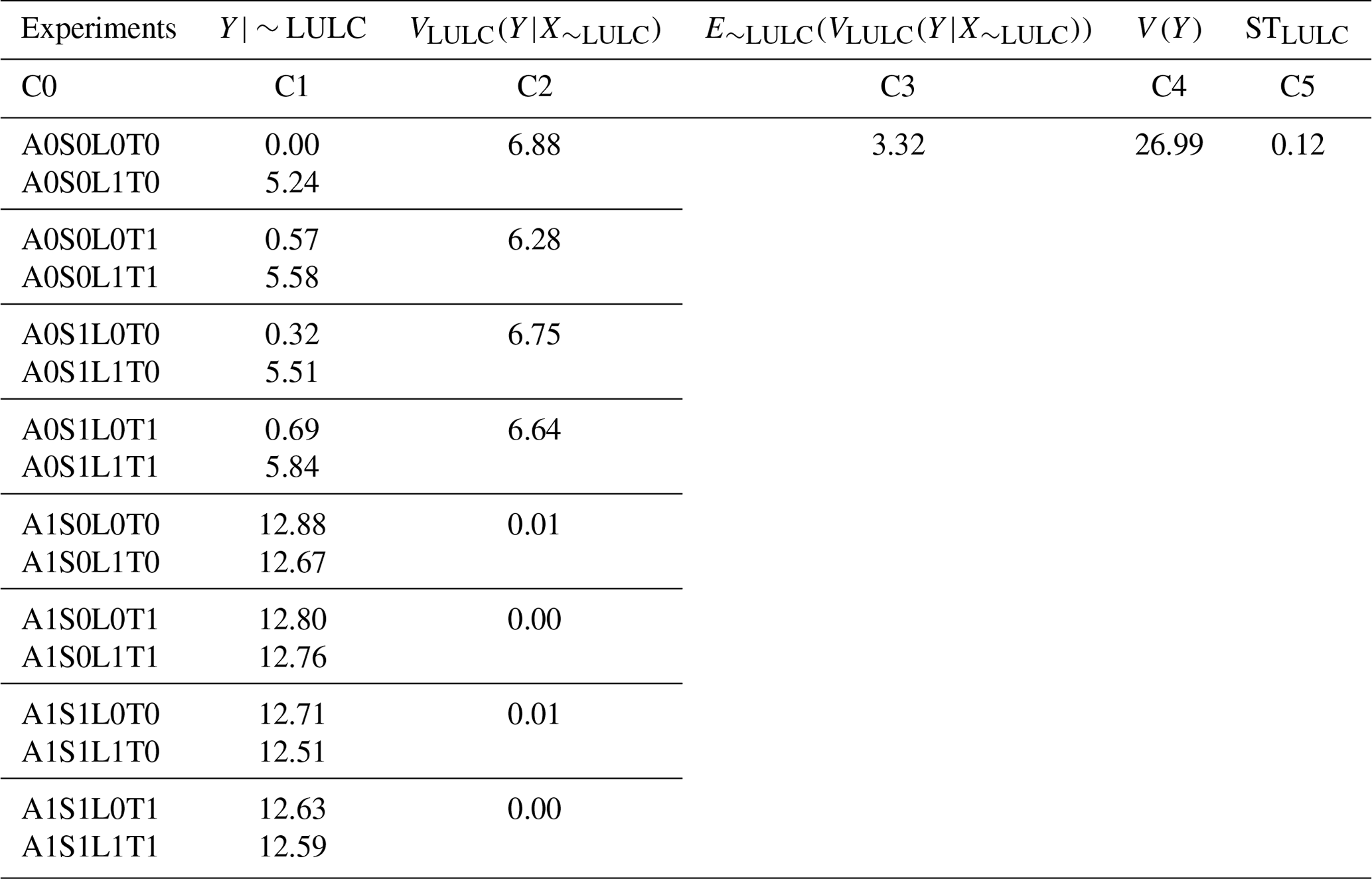
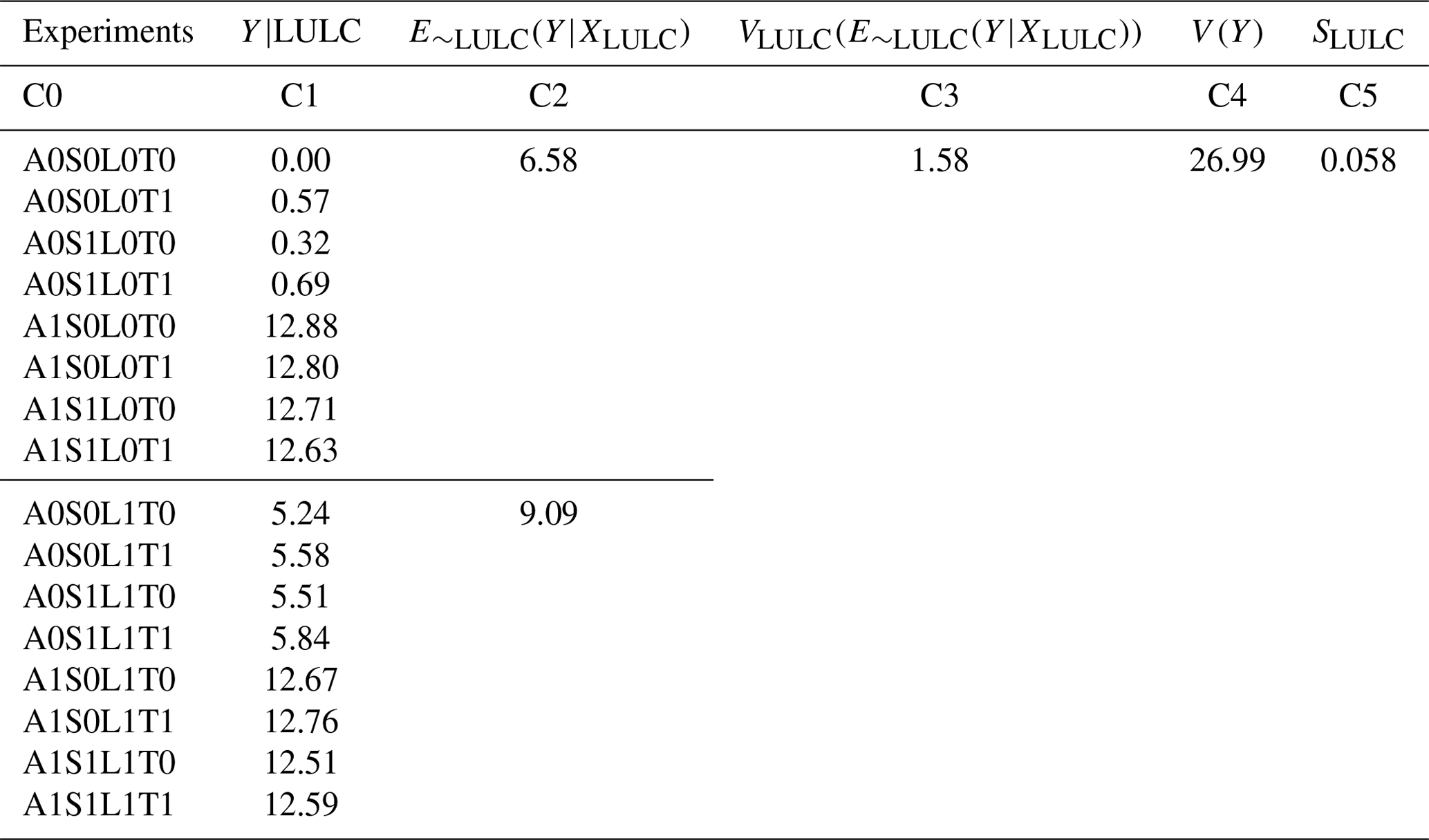
Table A3 Calculation of Sobol' interaction effect index and contributing fractions.

Appendix B: Spatial patterns of Sobol' total sensitivity index vs. SD ratio

To further understand the spatial patterns of the Sobol' total sensitivity index for the two most dominant heterogeneity sources of ATM and LULC (Fig. 5), we further analyzed EXP9 (A1S0L0T0) and EXP3 (A0S0L1T0) listed in Table 2. EXP9 and EXP3 only include heterogeneous inputs from ATM and LULC, respectively. Let us consider $\text{ET}/P$ as the quantity of interest for the following discussion. First, the SD of $\text{ET}/P$ is computed from the annual climatology (Sect. 2.3). Next, the SD ratio of $\text{ET}/P$, denoted as ${\text{SDR}}_{\text{ET}/P}$, is computed as the ratio between the SD of $\text{ET}/P$ in EXP9 and EXP3. ${\text{SDR}}_{\text{ET}/P}$ represents the relative spatial variability induced by ATM compared to LULC (Fig. B1a). The spatial pattern of the ATM Sobol' total sensitivity index for the $\text{ET}/P$ spatial variability shows a positive relationship with the spatial pattern of ${\text{SDR}}_{\text{ET}/P}$ (purple circles in Fig. B1d, corresponding to Fig. 5a vs. Fig. B1a). Therefore, a higher value of ${\text{SDR}}_{\text{ET}/P}$ indicates that relative to LULC, ATM induces larger $\text{ET}/P$ spatial variability and, hence, has a higher ATM Sobol' total sensitivity index. Similarly, a lower value of ${\text{SDR}}_{\text{ET}/P}$ indicates LULC induces larger $\text{ET}/P$ spatial variability than ATM and, hence, has a higher LULC Sobol' total sensitivity index (green circles in Fig. B1d). Similarly, ${\text{SDR}}_{R/P}$ and SDR_EF were calculated for $R/P$ and EF, and they also show a positive (negative) relationship with the corresponding ATM (LULC) Sobol' total sensitivity index (Fig. B1b, c, e, and f). We can also see that the ATM Sobol' total sensitivity index has opposite spatial patterns compared to the LULC Sobol' total sensitivity index. Therefore, ATM and LULC show complementary contributions to the spatial variability of water and energy partitioning across CONUS.

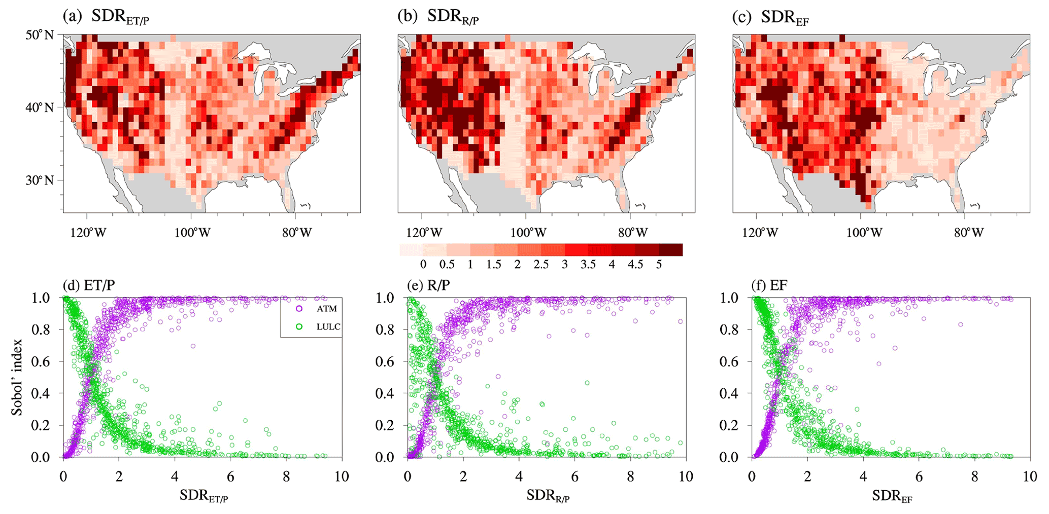
Figure B1 Spatial patterns of SD ratios (a–c) and their spatial relationship with the ATM and LULC Sobol' total sensitivity index (d–f) for $\text{ET}/P$, $R/P$ and EF, respectively. The y axis values correspond to the spatial patterns of the Sobol' total sensitivity index for ATM (purple) and LULC (green) in Fig. 5 (i.e., each circle corresponds to each 1^∘ × 1^∘ region).

Appendix C: Seasonal variations of Sobol' total sensitivity index vs. normalized SD ratio

To further explain the seasonal variations of the Sobol' total sensitivity index for ATM and LULC, the SD of ET for each month was calculated as an example from monthly mean climatology. The SD ratio for each month was computed as the ratio between the SD of ET in EXP9 and EXP3. For each 1^∘ × 1^∘ region, the 12 monthly SD ratios were normalized to [0, 1] using minimum and maximum values. Finally, the CONUS average of the normalized SD ratios was computed for each month, denoted as NSDR_ET. A higher value of NSDR_ET denotes ATM induces more ET spatial variability than LULC. Therefore, NSDR_ET shows similar seasonal variations with the ATM Sobol' total sensitivity index for ET spatial variability (black curve vs. purple curve in Fig. C1a), but opposite seasonal variations with the LULC Sobol' total sensitivity index (black curve vs. green curve in Fig. C1a). Similarly, normalized SD ratios were calculated for R, SH, ET components, and R components, and they also show a similar (opposite) seasonal variation with the corresponding seasonal ATM (LULC) Sobol' total sensitivity index (Fig. C1).

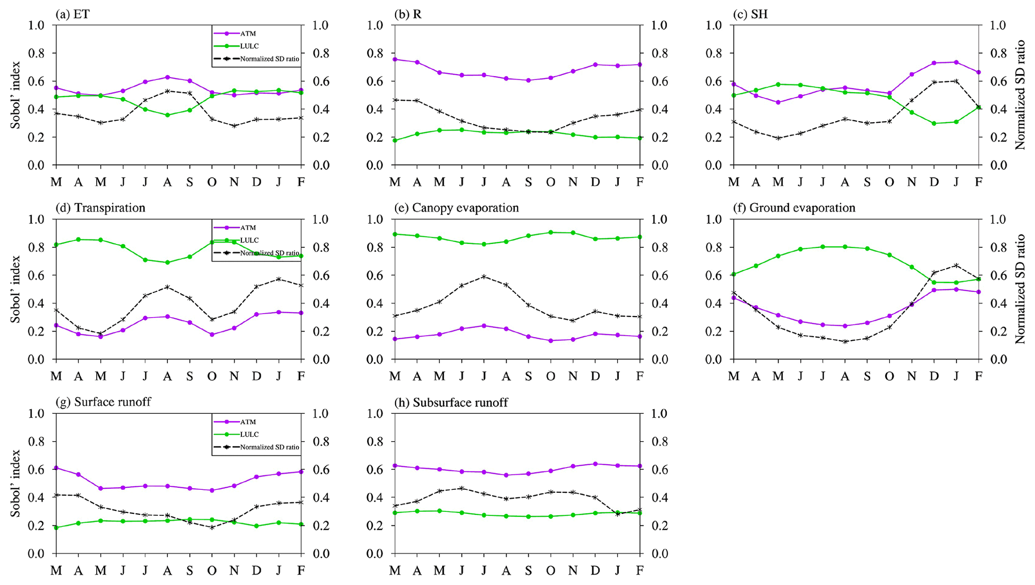
Figure C1 Monthly variations of CONUS-averaged ATM and LULC Sobol' total sensitivity index to ATM and normalized SD ratio for (a) ET, (b) R, and (c) SH, (d) transpiration, (e) canopy evaporation, (f) ground evaporation, (g) surface runoff, and (h) subsurface runoff, respectively.