the Creative Commons Attribution 4.0 License.
the Creative Commons Attribution 4.0 License.
 | 19 Jul 2022
Atmospheric river representation in the Energy Exascale Earth System Model (E3SM) version 1.0
Sol Kim
L. Ruby Leung
Bin Guan
John C. H. Chiang
The Energy Exascale Earth System Model (E3SM) project is an ongoing, state-of-the-science Earth system modeling, simulation, and prediction project developed by the US Department of Energy (DOE). With an emphasis on supporting the DOE's energy mission, understanding and quantifying how well the model simulates water cycle processes is of particular importance. Here, we evaluate E3SM version 1.0 (v1.0) for its ability to represent atmospheric rivers (ARs), which play significant roles in water vapor transport and precipitation. The characteristics and precipitation associated with global ARs in E3SM at standard resolution (1∘ × 1∘) are compared to the Modern-Era Retrospective analysis for Research and Applications, version 2 (MERRA2). Global patterns of AR frequencies in E3SM show high degrees of correlation (≥0.97) with MERRA2 and low mean absolute errors (MAEs; <1 %) annually, seasonally, and across different ensemble members. However, some large-scale condition biases exist, leading to AR biases – most significant of which are the double intertropical convergence zone (ITCZ), a stronger and/or equatorward-shifted subtropical jet during boreal and austral winters, and enhanced Northern Hemisphere westerlies during summer. By comparing atmosphere-only and fully coupled simulations, we attribute the sources of the biases to the atmospheric component or to a coupling response. Using relationships revealed in Dong et al. (2021), we provide evidence showing the stronger North Pacific jet in winter and the enhanced Northern Hemisphere westerlies during summer, associated with E3SM's double ITCZ and related weaker Atlantic meridional overturning circulation (AMOC), respectively, which are significant sources of the AR biases found in the coupled simulations.
- Article
(15218 KB) - Full-text XML
- BibTeX
- EndNote


Atmospheric rivers (ARs) are central actors in the global water cycle and have significant human impacts. These features are narrow, filamentary structures of concentrated water vapor transport in the lower atmosphere, responsible for transporting the majority of water vapor across the midlatitudes towards the poles (Zhu and Newell, 1998). Recently, ARs have received a categorization similar to hurricanes, which describes the wide range of possible AR impacts – both beneficial and destructive (Ralph et al., 2019). Weaker ARs, with integrated vapor transport (IVT) values of around 250 kg m−1 s−1, can provide regions such as the west coast of the US with critical sources of precipitation, while exceptional ARs, with IVT values well over 1250 kg m−1 s−1, can be associated with widespread flooding and hazards to both human life and infrastructure. A recent study examining the last 40 years of floods in the western US found that ARs pose a USD 1 billion-a-year flood risk (Corringham et al., 2019). Many studies indicate that ARs will increase in frequency and/or intensity and will deliver more precipitation under global warming (e.g., Payne and Magnusdottir, 2015; Espinoza et al., 2018; Payne et al., 2020; O’Brien et al., 2021). On the west coast of the US for example, ARs are expected to increase the occurrence of extreme precipitation and associated flood risk, including their contribution to snow/ice melt (Swain et al., 2018; Chen et al., 2019). With such important socioeconomic impacts, increasing our understanding of ARs in past, present, and future climates is critical to mitigate damage and protect life and property.
Although ARs have been directly observed since the late 1990s with aircraft and dropsondes, e.g., the California Land-falling Jets Experiment (CALJET) (Ralph et al., 2005), and via satellites with passive microwave radiometers (Ralph et al., 2004; Ralph et al., 2006), gaps and challenges to direct observations of ARs still exist due to both the scale and the extreme environments associated with ARs. While efforts to directly observe ARs continue to be improved, much of these efforts to date have been regionally specific to the western US, where ARs play a critical role in water resources. Thus, many researchers have instead relied on the use of gridded reanalysis products – which incorporate a variety of observations – to study ARs in historical, regional, and global perspectives (Ralph et al., 2020). Given the socioeconomic impacts of ARs, there is also wide and increasing interest on the behavior of ARs in future climates, which typically require the use of global climate models (GCMs) (e.g., Dettinger et al., 2011; Payne and Magnusdottir, 2015; Warner et al., 2015; Shields and Kiehl, 2016). A critical step in using these GCMs, which are used to simulate ARs in a variety of climates, is to first establish confidence in the model's ability to simulate ARs in the current climate.
Many efforts have already evaluated a large array of different models. For example, Guan and Waliser (2017) evaluated 22 GCMs that participated in the Global Energy and Water Cycle Experiment (GEWEX) Atmospheric System Study (GASS)-Year of Tropical Convection (YoTC) multimodel experiment, which included both atmosphere-only and ocean–atmosphere-coupled models for the 1991–2010 period. They used reanalysis products to quantify model errors in the context of reanalysis uncertainty and found large errors across all models. Another study by Espinoza et al. (2018) evaluated 21 GCMs in the Coupled Model Intercomparison Project Phase 5 (CMIP5) for their representation of ARs in historical and two future climates, i.e., Representative Concentration Pathway (RCP) 4.5 and 8.5. The multimodel mean (MMM) was a good representation of their reference dataset, ERA-Interim but tended to have a general underestimation of AR frequencies in the midlatitudes. Additionally, intermodel differences showed significant disagreement for AR frequencies in the subtropics. Payne and Magnusdottir (2015) performed a similar analysis on land-falling ARs to understand responses to warming in RCP8.5, and compared CMIP5 historical runs to both ERA-Interim and the Modern-Era Retrospective analysis for Research and Applications (MERRA) as an initial step. Most models were able to resolve the general shape of winter land-falling AR frequencies, but only a few could resolve other characteristics such as interannual variability in amplitude of moisture flux and median land-falling latitude. A strong relationship between model biases in the North Pacific subtropical jet and land-falling AR frequency on the west coast of North America has been identified based on analysis of large ensemble simulations from the Community Earth System Model (CESM) (Hagos et al., 2016). More recently, O’Brien et al. (2021) evaluated several CMIP5 and CMIP Phase 6 (CMIP6) models' historical simulations (prior to evaluating a projection scenario) against MERRA2, and found frequency distributions to be remarkably consistent.
The US Department of Energy (DOE) recently released the Exascale Energy Earth System Model version 1 (E3SMv1), which is a state-of-the-science Earth system model. The model was developed to support the DOE's energy mission, with an emphasis on modeling the long-term changes in air and water temperatures, water availability, storms and heavy precipitation, coastal flooding, and sea-level rise on high-performance computers (Leung et al., 2020). The standard resolution model (1∘ × 1∘) has been shown to credibly simulate Earth's climate when evaluated by means of a standard set of CMIP6 Diagnosis, Evaluation, and Characterization of Klima (DECK) simulations, which include a pre-industrial control, historical simulations, and idealized CO2 forcing simulations (Golaz et al., 2019). A suite of atmospheric fields (e.g., net top-of-the-atmosphere radiation, surface air temperature, zonal winds, and precipitation) in the historical E3SMv1 simulations were compared against observations to calculate root mean square errors (RMSEs). When compared to an ensemble of 45 CMIP5 models, E3SMv1's RMSEs were generally found to have lower errors than the median of the CMIP5 ensemble, and for many fields and seasons, in the lowest (best) quantile. There are however, known biases in E3SMv1 which are common to other GCMs, such as a reduction in cloudiness over the subtropical stratocumulus regions and the well-known double intertropical convergence zone (double ITCZ) issue where there is excessive southern central Pacific precipitation (Zhang et al., 2007; Golaz et al., 2019).
Evaluating E3SMv1 for ARs, which has not yet been done, is necessary given our need to understand issues surrounding the water cycle and its interactions with humans and other Earth systems. This paper aims to provide an overview of ARs simulated in E3SMv1 by (i) comparing it against historical ARs detected in MERRA version 2 (MERRA2) to identify AR biases, (ii) evaluating internal model AR variability using individual ensemble members, and (iii) determining the large-scale and model sources of AR biases. ARs in this study are detected using the AR algorithm developed by Guan and Waliser (2019) which is a widely used algorithm and has been demonstrated to closely match key AR characteristics from direct airborne observations (Guan et al., 2018). The structure of this paper is as follows: in Sect. 2, E3SMv1, the reanalysis dataset, and the AR detection algorithm are described. The AR frequency, characteristics, precipitation, and large-scale conditions in E3SMv1 are compared to MERRA2 in Sect. 3. Discussion and conclusions are presented in Sect. 4. Appendix material are contained in Sect. A.
2.1 Exascale Energy Earth System Model
The E3SMv1 was developed from CESM (Leung et al., 2020). This study uses global, daily mean data from the standard 1∘ × 1∘ resolution (also referred to as the “low” resolution), fully coupled E3SMv1 (Golaz et al., 2019). We use 35 years (1980–2014) of historical simulation which incorporates several historical, observed forcings, including atmospheric composition changes. Five ensemble members of historical simulations are available from E3SMv1 in the CMIP6 archive; these five members use initial conditions from the pre-industrial control run, branched out at 50-year intervals, beginning with 1 January of year 101. The ensemble members are used in this study to examine internal variability related to ARs and to generate ensemble mean frequencies of ARs. The E3SM Atmosphere Model (EAM) (Rasch et al., 2019), which was developed from the Community Atmosphere Model version 5 (CAM5), uses a spectral element dynamical core, and is applied at a horizontal resolution of approximately 110 km (or 1∘ × 1∘; 180 latitude grids × 360 longitude grids), and has 72 vertical levels. The historical runs follow the CMIP6 protocols outlined in Eyring et al. (2016). To understand the sources of model biases in simulating ARs, we also analyze atmosphere-only simulations for comparison with the fully coupled historical simulations, as has been done in previous studies to identify sources of errors (e.g., Li and Xie, 2012; Li and Xie, 2014). The atmosphere-only simulations follow the Atmospheric Model Intercomparison Project (AMIP) protocol and are part of the CMIP6 DECK simulations. All three available AMIP ensemble members are used in this study and atmosphere, and land initial conditions for these ensemble members were taken at year 1870 from the first three historical ensemble members. The AMIP simulations have prescribed sea surface temperatures (SSTs) and sea-ice concentrations from observations. A full overview of E3SMv1 and EAM can be found in Golaz et al. (2019) and Rasch et al. (2019), respectively. We will henceforth refer to E3SMv1 as E3SM. The fields obtained from E3SM are total (vertically integrated) zonal/meridional water flux, total (convective and large-scale) precipitation rate (liquid + ice), total (vertically integrated) precipitatable water, zonal wind at 200 hPa, and geopotential height at 500 hPa.
2.2 Reanalysis dataset
In this study, daily mean reanalysis data from MERRA2 (Gelaro et al., 2017) is analyzed for the same 35-year period as E3SM (1980–2014). The native spatial resolution is ∼ 50 km (or 0.5∘ × 0.625∘; 361 latitude grids × 576 longitude grids) but was regridded to match E3SM and facilitate comparison. MERRA2 is an updated version of MERRA (version 1) which was developed to improve representations of the global water cycle. Good agreement between MERRA2 against airborne and satellite observations has been previously demonstrated for ARs (Ralph et al., 2012; Guan et al., 2018). In addition, MERRA2 has been used extensively in previous AR studies (e.g., Shields et al., 2018; Rutz et al., 2019). The fields obtained from MERRA2 are the same as those obtained from E3SM but can correspond to different long names: eastward/northward flux of atmospheric water vapor, total precipitation, atmosphere–water vapor content, eastward wind at 200 hPa, and geopotential height at 500 hPa.
2.3 AR detection algorithm
The ARs are detected using tARget v3 – the latest version of a widely used algorithm developed for global studies. Details of the detection algorithm can be found in Guan and Waliser (2015), Guan et al. (2018), and Guan and Waliser (2019). This algorithm is part of the Atmospheric River Tracking Method Intercomparison Project (ARTMIP) (Shields et al., 2018), and is among the relatively “permissive” algorithms, compared to other algorithms, that facilitate global analyses including inland-penetrating ARs as well as polar ARs but meanwhile effective in filtering out non-AR features in the tropics. While there is significant uncertainty associated with the choice of detection algorithm (Shields et al., 2018; Shields et al., 2019; O’Brien et al., 2020; Rutz et al., 2019), we choose to use this algorithm for its global applicability, and make no attempt in this study to quantify the uncertainty as this is a primary goal of ARTMIP. The algorithm, when applied to contemporary reanalysis products, detected ARs that were found to closely match airborne observations in terms of key characteristics, such as AR width and total IVT across AR width (Guan et al., 2018). Various refinements and improvements have been made to the algorithm's current version since it was first introduced in Guan and Waliser (2015). As a brief summary, the algorithm extracts contiguous areas of connected grid points, based on IVT exceeding location- and season-specific IVT thresholds set at the 85th percentile of the dataset analyzed but cannot go below 100 kg m−1 s−1. Geometric and directional requirements are then applied to the identified objects, with considerations of the direction of the object mean IVT (poleward component >50 kg m−1 s−1), coherence of IVT directions (more than half of the area having an IVT direction within 45∘ from the object mean IVT), length (>2000 km), and length/width ratio (>2) (Guan and Waliser, 2019). The IVT threshold is calculated separately for MERRA2 and the E3SM simulations. We include the annual mean 85th percentile IVT of both along with the differences in Sect. A (Fig. A2). In general, E3SM has higher threshold IVT values than MERRA2, with some regional biases up to 100 kg m−1 s−1. Notably, these high positive IVT bias regions are over the subtropical jet in the Northern Hemisphere (which we discuss throughout the paper), and the midlatitude jet in the Southern Hemisphere where there are known warm SST biases (Golaz et al., 2019) and associated enhanced atmospheric moisture (not shown).
3.1 AR frequency
We begin with the global distribution of AR frequencies shown in Fig. 1. These frequencies represent the ensemble mean from five historical simulations for E3SM compared to MERRA2. The AR detection algorithm was applied to each ensemble member individually to calculate the ensemble mean. For each grid cell, the frequency shown represents the number of time steps the grid cell was part of, and AR divided by the total number of time steps in the time period. This is done for the annual, extended boreal winter (NDJFM), and extended boreal summer (MJJAS). The distribution of the annual frequency of ARs in E3SM closely matches MERRA2's distribution as seen in Fig. 1a and b. In E3SM, as in MERRA2, frequency maxima are found in the extratropics over the Pacific, Atlantic, and South Indian ocean basins, while minima can be seen along the Equator, at high polar latitudes, and over both Greenland and the Tibetan Plateau. The difference of E3SM minus MERRA2 annual frequencies is shown in Fig. 1c. To note, in the annual (seasonal) period, 1 % of absolute difference translates to 3.65 (∼ 1.5) time steps of AR difference out of 365 (151–153) time steps in a year (extended season). All percentage differences mentioned below, unless otherwise noted, are absolute differences, not relative differences. We include the relative differences of regions with absolute AR frequencies of at least 3 % in Sect. A (Fig. A2). Overall in E3SM, there are no-to-weak biases (<1 % absolute differences) over the AR frequency maxima regions, which translate to correspondingly low relative biases. Positive biases of higher magnitudes (1 %–3 %) are seen near the edge of the tropics and subtropics in both the Northern and Southern hemispheres. The E3SM also has positive biases in polar areas, specifically over Alaska, Siberia, and just offshore of Antarctica. These absolute AR frequency differences translate to relative differences of up to 60 % along the subtropical edge of the Pacific, over India, over the polar areas near Alaska, and off the Antarctic coast (Fig. A2c). These relative differences, while large, are over regions with annual AR frequencies of 5 % or less (with the exception of Alaska), where AR activity is expected to be particularly sensitive to large-scale conditions, and we explore contributing factors to these biases, particularly to the Pacific storm track region, in Sect. 3.4. Negative biases (1 %–2 %) are seen in the Southern Hemisphere subtropics (southwestern region of Australia and over the South Atlantic, east of Brazil). Between the E3SM ensemble mean and MERRA2, the annual frequency mean absolute error (MAE) is 0.60 % and the correlation is 0.98, showing strong agreement in the distribution and magnitude of global AR frequencies.
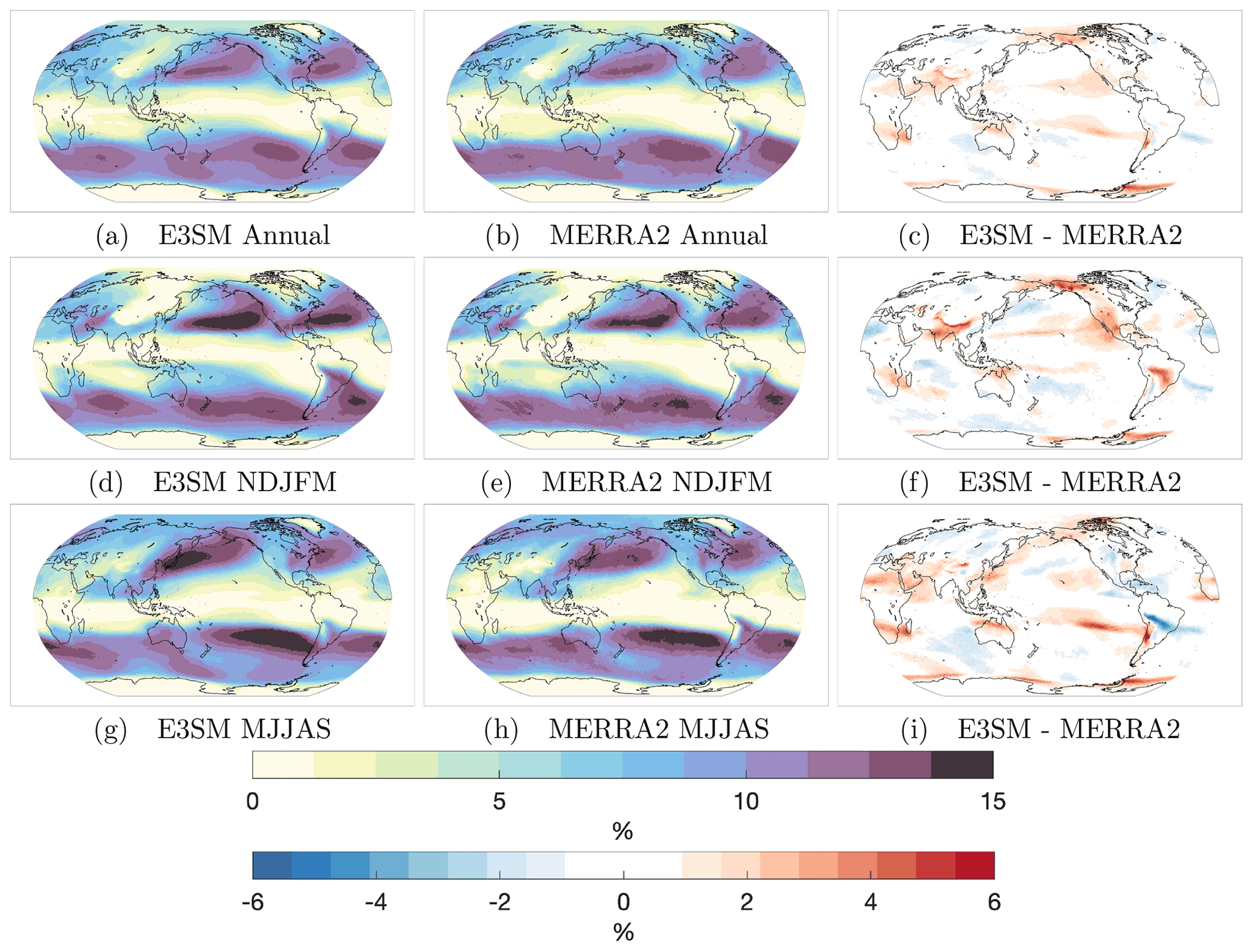
Figure 1The AR frequency at each grid point globally for the annual (a–c), extended winter NDJFM (d–f), and extended summer MJJAS (g–i) periods. The E3SM frequencies (a, d, g), MERRA2 frequencies (b, e, h), and the difference in frequencies between E3SM and MERRA2 (c, f, i). The color bar at the top (bottom) corresponds to the absolute (difference in) frequencies.
For NDJFM, E3SM (Fig. 1d) has AR frequency maxima and minima over regions matching MERRA2 (Fig. 1e), but there are areas with seasonal biases (Fig. 1f). The ARs are most frequent over the subtropics and midlatitudes over the North and South Pacific and Atlantic, where the storm tracks are located. One of the biggest sources of positive biases comes from North Pacific ARs, affecting the entire west coast of North America with frequencies around 3 %–4 % higher than in MERRA2. The relative differences in this region can reach up to 30 %–50 % (Fig. A2a) and lead us to investigate biases of the North Pacific subtropical jet in E3SM compared to MERRA2 in Sect. 3.4. These positive biases stretch from Mexico to Alaska, nearly uninterrupted as well as nearly all the way across the subtropical North Pacific basin. Other positive biases exist over South America (originating from the Amazon rainforest) and over India near the Himalayas, with high relative differences (>50 %). Negative anomalies of ∼ 1 %–2 % are seen throughout the Southern Hemisphere ocean basins as well as over northern Africa and east of Japan. The NDJFM frequency MAE is 0.72 % and the correlation is 0.98.
The MJJAS frequencies in E3SM (Fig. 1g), similar to NDJFM frequencies, have maxima and minima colocated with MERRA2's MJJAS frequencies (Fig. 1h) but, again, with some biases (Fig. 1i). Frequency maxima can be seen in both E3SM and MERRA2 over the western areas of the North Pacific and North Atlantic basins, and over the South Pacific and South Atlantic in the subtropics and midlatitudes. Positive biases are seen for E3SM in the following areas: the southern edge of the tropics near 15∘ S, with the exception of the negative frequency bias over South America, the Middle East, the western boundary of the North Pacific, windward side of the Andes, and offshore of Antarctica. The regions where these absolute differences translate to large relative differences are around 15∘ S (exceeding 100 % at the tropical edges), over the Arabian Sea (25 %–60 %), and offshore of Antarctica (exceeding 100 % closer to shore). Negative biases are overall weaker and are found over South America on the leeward side of the Andes (between ∼ 10–20∘ S), the Caribbean Sea, south Indian Ocean, and at midlatitudes and polar latitudes over Eurasia. The MJJAS frequency MAE is 0.82 % and the correlation is 0.97.
To summarize, E3SM and MERRA2 AR frequencies show very high correlation (≥0.97) and low MAEs (<1 %) annually and seasonally. The magnitude and distribution of annual and seasonal AR frequencies are consistent with previous studies examining ARs in reanalyses (e.g., Guan and Waliser, 2015; DeFlorio et al., 2019). However, in E3SM, the hemisphere experiencing winter (especially the Northern Hemisphere) tends to produce positive frequency biases, and corresponding large relative differences, throughout the border of the tropics and subtropics (∼ 25∘ N and ∼15∘ S). The Northern Hemisphere's summer features notable positive anomalies throughout the tropics/subtropics over the Middle East and along the western boundary of the North Pacific. Additionally, AR frequencies are higher near some elevated topography (such as the Himalayas, the Alaska Range, and Antarctica).
While the previous results are based on the five-member ensemble mean, we next determine how well the individual historical E3SM ensemble members are able to match MERRA2's AR frequencies using Taylor diagrams (Fig. 2). Taylor diagrams provide a graphical summary of similarity between two patterns using pattern correlation, centered root mean square difference (RMSD), and standard deviation (SD). The Taylor diagrams confirm E3SM's ability to accurately simulate present-day AR frequencies globally, across ensemble members, in the annual and seasonal periods with a high degree of similarity to MERRA2. Correlations are above 0.95 for all ensemble members and for the three periods analyzed (NDJFM, MJJAS, and annual), with the annual period having the highest correlation. The E3SM SDs are consistent with MERRA2's SD; all ensemble members, for all periods, are within 0.18 % of MERRA2. The RMSDs in the annual period are under 1.0 %, while they are under 1.5 % in the seasonal periods. The diagrams also suggest that the internal variability of the E3SM historical simulations is small – particularly in the annual period – as the five ensemble members are tightly clustered.
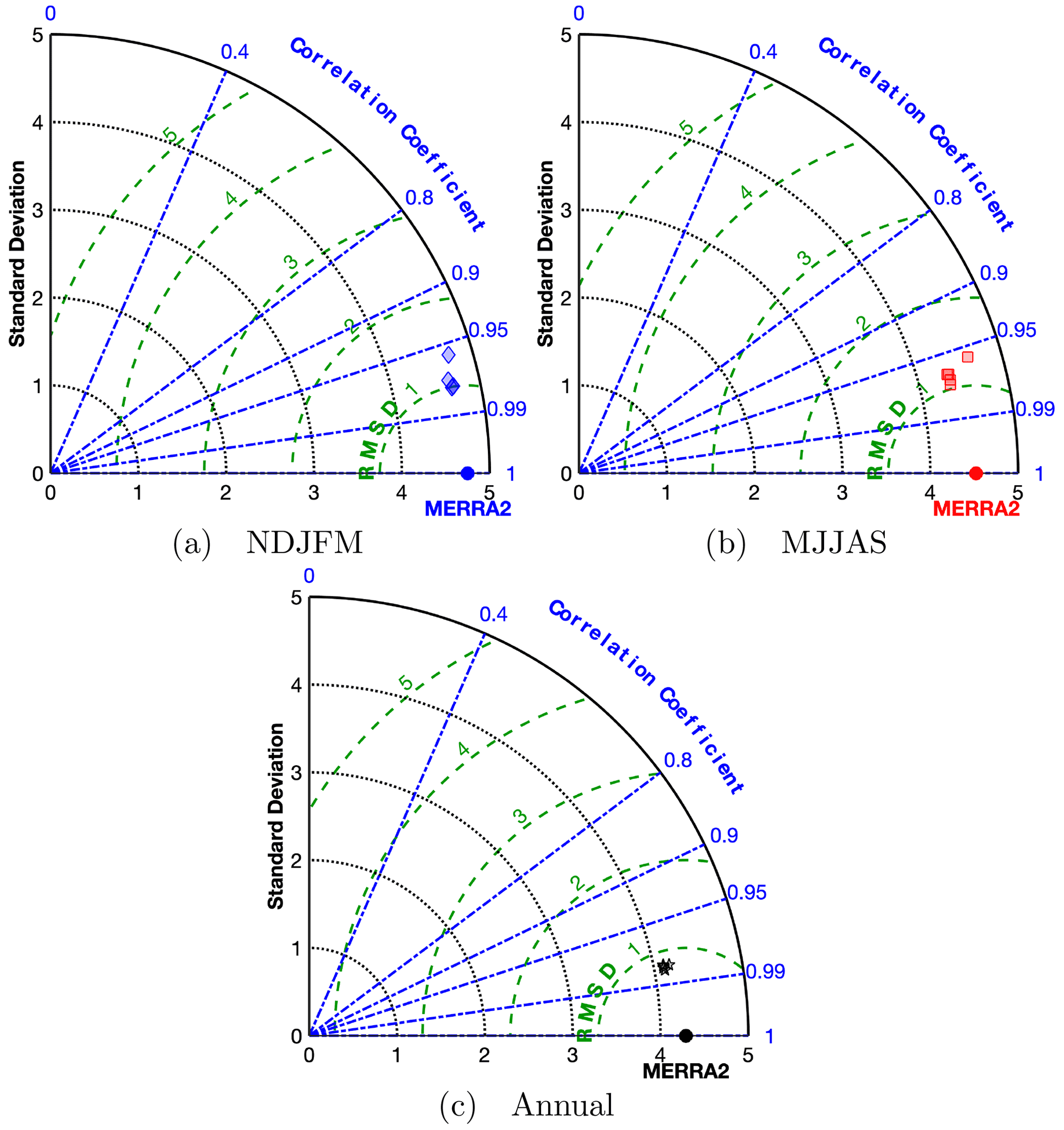
Figure 2Taylor diagrams of AR frequency for the five-ensemble historical E3SM members against MERRA2 for the (a) NDJFM, (b) MJJAS, and (c) annual periods. The MERRA2 point is labeled in each graph.
As a measure of ensemble spread, the five-member ensemble SD (different to the Taylor Diagram SD) of AR frequency – i.e., how much variance there is between the individual simulations and the ensemble mean – is shown in Fig. 3. For the annual period (Fig. 3c), much of the global SDs are below 0.5 %. A few regions, such as over East and Southeast Asia, the Arabian Sea, and the Hudson Bay, have SDs that fall between 0.5 % and 1.0 %. Analysis of the coefficient of variation (not shown), calculated at each grid globally as the ratio between ensemble AR frequency SD and mean ensemble frequency, shows that the annual SDs are well below 10 % of the ensemble mean AR frequencies for virtually all grid points, barring a few grid points over the Equator and Antarctica where ARs are very rare (annual frequencies are <1.0 %).
During NDJFM (Fig. 3a), SDs are generally higher in the Northern Hemisphere and have notable peaks of ∼ 1.5 % over East Asia (which is a jet entrance region) and the North Pacific storm track region. These regional peaks suggest that differences in subtropical jet behavior during NDJFM, between the five historical simulations, may be responsible for some of the internal AR frequency variability. The MJJAS SDs (Fig. 3b) have maxima of ∼ 1.5 % over various regions of the Asia summer monsoon - the Arabian Sea, over the Philippines, and East Asia. This suggests that during MJJAS, differences in monsoon, Madden–Julian Oscillation (MJO), or subtropical jet behavior, may drive AR frequency variability between various E3SM ensemble members. In general, the Northern Hemisphere shows more internal variability; likely due to both internal interannual and interdecadal variability of the midlatitude circulation in the region and especially in the North Pacific.

Figure 3The historical E3SM five-member ensemble standard deviation (SD) of AR frequencies for the (a) winter, (b) summer, and (c) annual periods.
3.2 AR characteristics
Next, we examine several AR characteristics in E3SM (using a single historical simulation) and MERRA2. These characteristics are provided by the AR detection algorithm's output for each individual AR. The distributions for the various AR characteristics are shown in Fig. 4. All characteristics show strong similarities in the distribution shape and peak in probability at the same bin values aside from the magnitude of mean IVT (Fig. 4e).

Figure 4Distributions of a variety of AR characteristics in E3SM and MERRA2. The yellow bars and solid line (median) are for E3SM and the blue bars and dotted line (median) are for MERRA2. Two sets of lines indicate hemispheric median values.
The length (Fig. 4a) and width (Fig. 4b) distributions of ARs in E3SM are generally consistent with MERRA2 as well as with previous characterizations of AR geometry (e.g., Guan and Waliser, 2015; Guan et al., 2018). The median length and width of ARs in E3SM are ∼ 3 % longer (3501 km compared to 3397 km) and wider (658 km compared to 639 km) than in MERRA2. The E3SM AR length/width ratio distribution and median (Fig. 4c) are in good agreement with MERRA2.
The hemispheric median centroid latitude of ARs is consistent, but the distributions reveal that E3SM produces more ARs with centroid latitudes in the tropics, subtropics, and southern polar latitudes, while producing fewer ARs in the midlatitudes compared to MERRA2 (Fig. 4d). These results are supported by the frequency differences in Fig.1.
The median magnitude of mean IVT of ARs in E3SM is 10.6 % larger than MERRA2 (Fig. 4e). The distribution of ARs peaks at 500 kg m−1 s−1 for E3SM but peaks at weaker magnitudes around 350 kg m−1 s−1 for MERRA2. These distribution differences reflect E3SM's positive IVT biases (Fig. A1c) in regions of high AR activity.
The direction of mean IVT (0∘ for IVT directed to the north) is directed towards the northeast (median angle of 65 and 62∘ for E3SM and MERRA2, respectively) in the Northern Hemisphere, and towards the southeast in the Southern Hemisphere (median angle of 120 and 123∘ for E3SM and MERRA2, respectively) (Fig. 4f). The E3SM ARs have higher probabilities around 90∘ (indicating a mean IVT directed to the east) and around 270∘ (indicating a mean IVT directed to the west). These median values, along with the distributions, indicate that E3SM ARs tend to have mean IVTs directed slightly more zonally compared to MERRA2. Coherence of IVT directions within an AR is calculated as the fraction of AR grid cells, with IVT directed within 45∘ of the mean AR IVT (Guan and Waliser, 2015). Model and reanalysis show similarly high coherences of 0.99 (E3SM) and 0.98 (MERRA2) (Fig. 4g).
3.3 AR precipitation
We now compare a variety of metrics related to AR precipitation. For reference, annual precipitation – not just from ARs – is included (Fig. 5a–c) for both models and reanalysis along with the differences. In this study, AR precipitation is defined as the precipitation that falls within an AR boundary.
For annual AR precipitation rates (Fig. 5d–f), E3SM is able to simulate the general global distribution and magnitude of AR precipitation characterized in previous studies using the Global Precipitation Climatology Project (GPCP) version 1.2 (e.g., Guan and Waliser, 2015; Ralph et al., 2020) as well as MERRA2 but with some differences. The E3SM has higher AR precipitation estimates over significant portions of the tropics and subtropics but lower estimates along the Equator (Fig. 5f), largely reflecting the pattern of general precipitation biases (Fig. 5c). The western coasts of North and South America also have higher rates of AR precipitation in E3SM. The seasonal differences in AR precipitation for NDJFM and MJJAS are largely consistent to the annual differences. We also include mean annual total precipitation (mm yr−1) for E3SM, MERRA2, and their difference (Fig. A3), to show how AR precipitation rate biases translate into annual quantities. The AR precipitation rate biases are important contributors to precipitation totals for regions outside of the tropics where ARs occur more frequently.
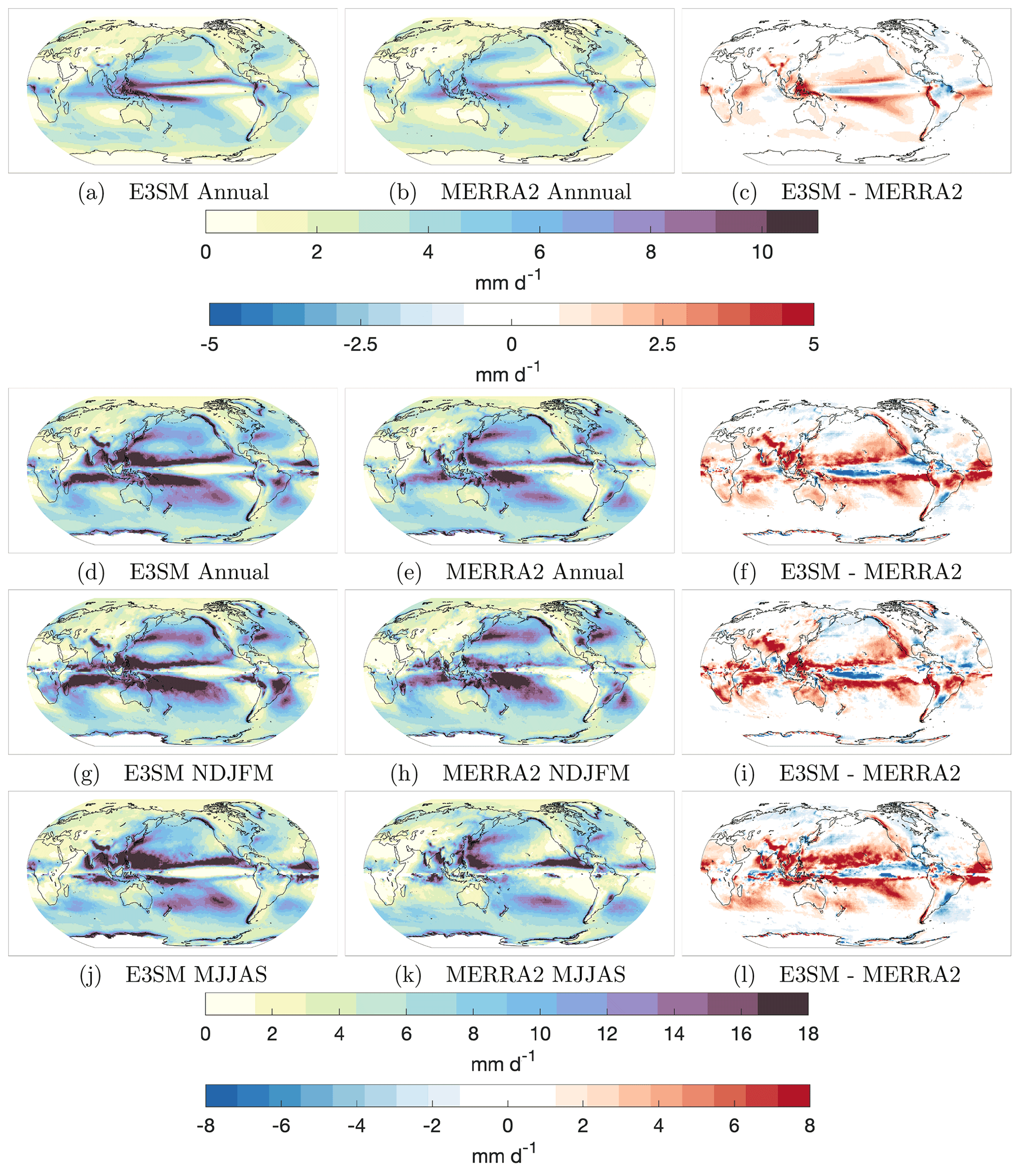
Figure 5Top row shows annual precipitation in E3SM, MERRA2, and the difference. The next three rows are organized as in Fig. 1 but for AR precipitation instead of AR frequency. The color bar at the top (bottom) corresponds to the absolute (difference in) precipitation or AR precipitation.
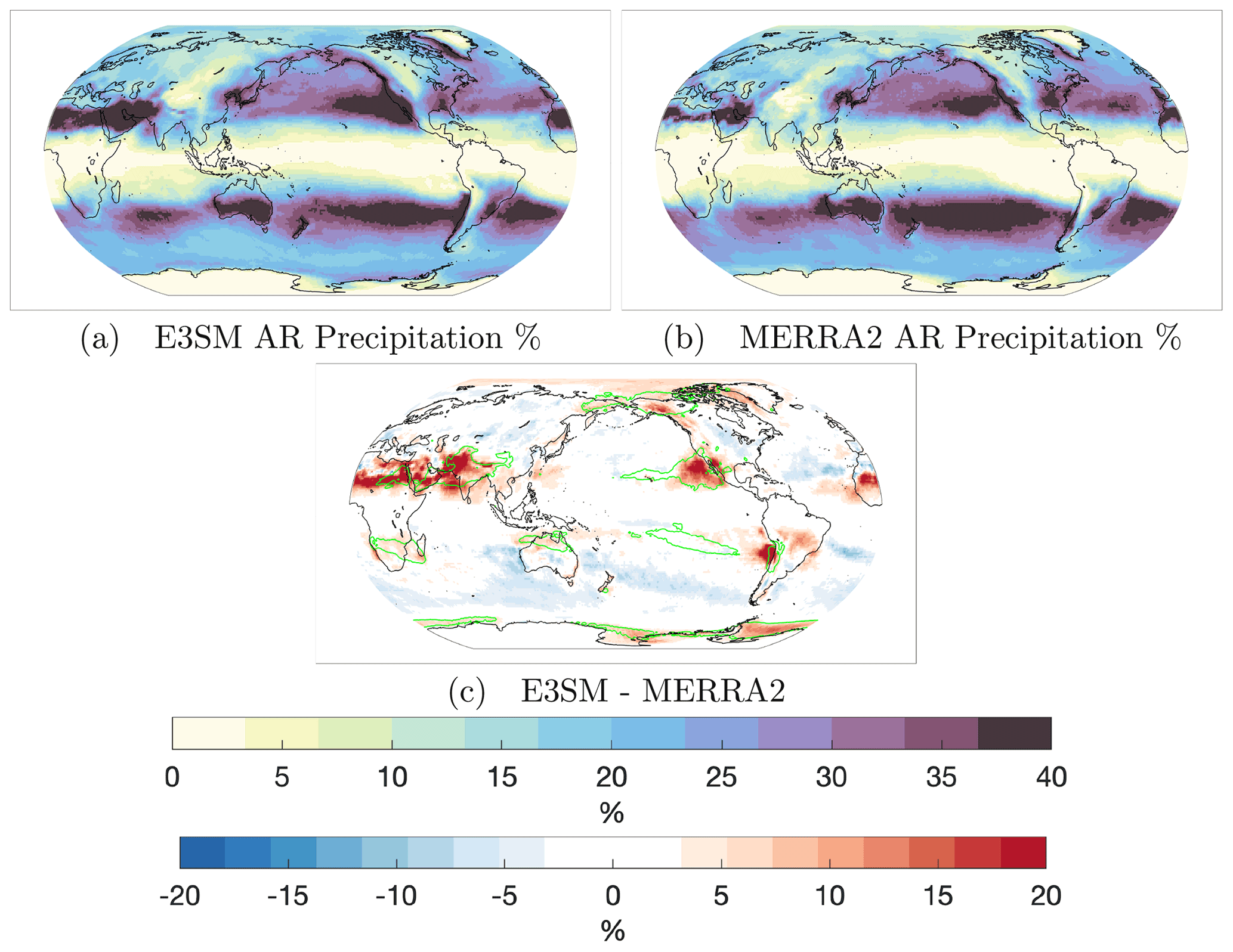
Figure 6The fraction of annual precipitation attributed to ARs for each grid cell for (a) E3SM and (b) MERRA2. The difference (E3SM minus MERRA2) is shown in (c). The color bar at the top (bottom) corresponds to the absolute (difference) percentages. Contour lines in (c) indicate the 1.5 % positive AR frequency biases from Fig. 1c.
Next, we examine the percentage of precipitation attributed to ARs in both datasets annually (Fig. 6). The ARs can be responsible for over 30 % of the annual precipitation in the expected extratropical areas such as the west coast of North and South America. Some other areas of note with high AR precipitation fractions include East Asia, the Middle East, southeastern US, Greenland, and Australia. These areas of high AR precipitation fractions have been characterized in previous studies (Guan and Waliser, 2015; Ralph et al., 2020). The precipitation fraction differences, shown in Fig. 6c, reveal that E3SM does, however, attribute a higher fraction of precipitation to ARs (up to 20 %) off the coast of southwestern US/Mexico and Chile. There is also a strong band of higher AR fractions (exceeding 20 %) extending from the Sahel/Sahara region of Africa, eastward to India. In addition, the polar regions exhibit higher AR fractions. Some midlatitude regions attribute less precipitation to ARs in E3SM, particularly over the oceans of the Southern Hemisphere. As expected, areas of higher AR precipitation fraction tend to be colocated with areas of positive AR frequency biases. Exceptions are Northeast Africa, the Arctic, and over the Amazon – all regions with low annual AR frequency biases; this suggests a small number of AR events are shifting the AR fractions in these locations.
Globally and annually, ARs are responsible for 17.84 % and 17.95 % of precipitation in E3SM and MERRA2,, respectively. Interestingly, while the overall precipitation percentage is very consistent, the fraction of AR precipitation that falls over ocean and land vary between the two datasets. In E3SM, 17.38 % (82.62 %) of the AR precipitation falls over land (oceans), while in MERRA2, only 14.81 % (85.19 %) falls over land (oceans). Topographic features seem to be able to extract precipitation from AR events more effectively in E3SM compared to MERRA2 – also evidenced by Fig. 5f.
3.4 Large-scale AR conditions
In this section, we look into the sources of the E3SM AR frequency and precipitation biases by examining the large-scale conditions relevant to ARs. We begin with the AR precipitation biases in the fully coupled E3SM simulations. The E3SM AR precipitation biases (Fig. 5f) are mostly well colocated and of similar magnitude with the general precipitation biases present in E3SM (Fig. 5c). While this reflects the important contributions of AR precipitation to the total precipitation in some regions, it also suggests that the AR precipitation and total precipitation biases can share similar sources of large-scale circulation biases. For example, model biases in the subtropical jet could affect precipitation produced by AR and non-AR storms, as both are influenced by the jet and storm tracks (Shields and Kiehl, 2016; Zhang and Villarini, 2018; Wahl et al., 2019; Ralph et al., 2020). Two notable exceptions where there are positive AR precipitation biases but no equivalent general precipitation biases are (i) southwest off the coast of the US and (ii) the region around Pakistan/India. These are the same regions in E3SM, compared to MERRA2, that attribute a higher fraction of the annual precipitation to ARs (Fig. 6), partly due to positive AR frequency biases. This suggests that certain large-scale circulation biases in these regions have a larger influence on AR frequency and intensity than the frequency/intensity of non-AR storms leading to a larger fraction of annual precipitation being delivered in the form of AR events rather than non-AR storms.
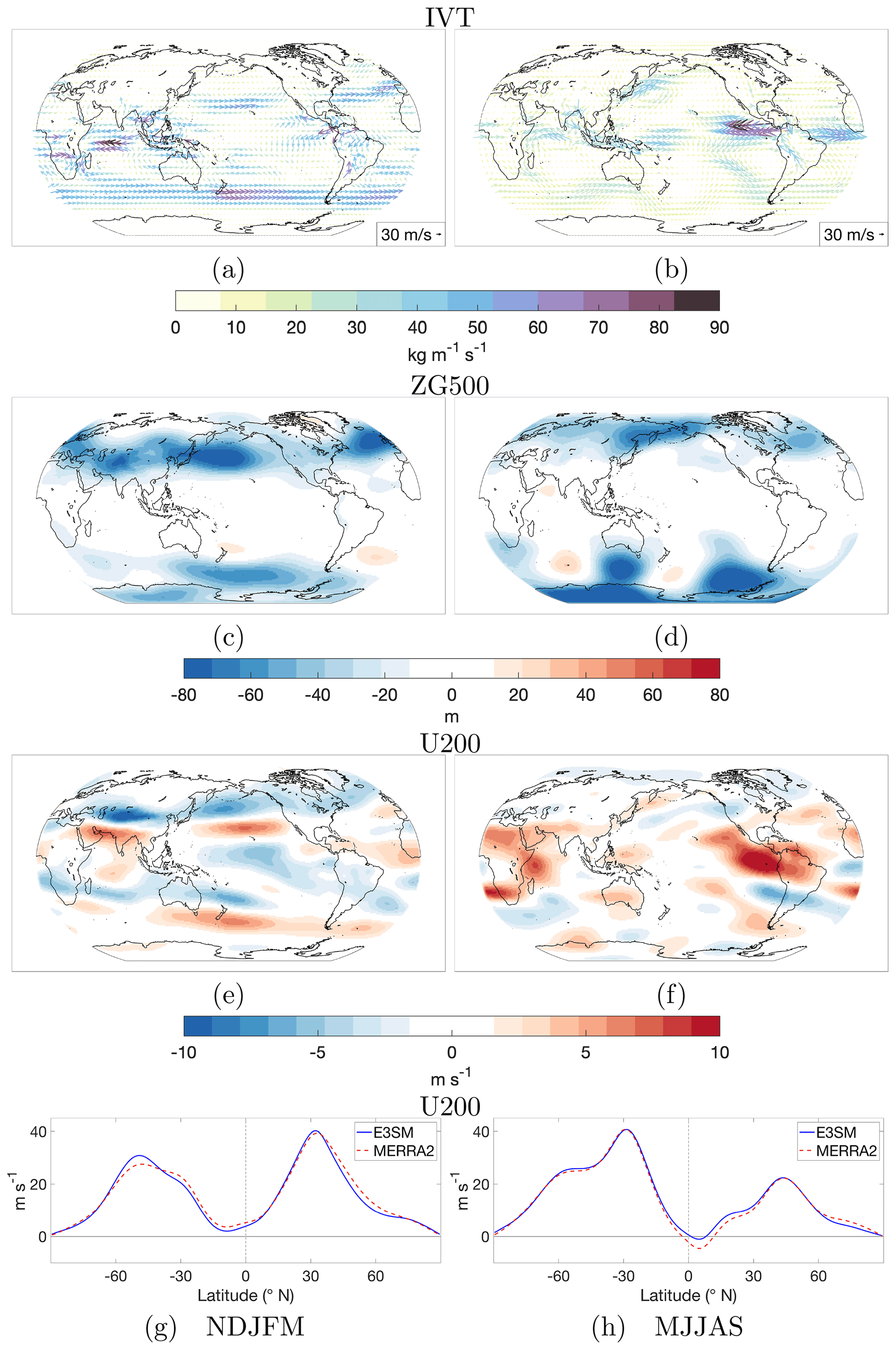
Figure 7Seasonal differences between E3SM and MERRA2 (a–h) – IVT, geopotential height at 500 hPa, zonal wind at 200 hPa, and zonal means over the Pacific and Atlantic basins (100–360∘ E) of zonal wind at 200 hPa.
A large source of general E3SM precipitation biases come from known and common biases in fully coupled simulations – the double ITCZ bias and excessive precipitation over the maritime continent (Golaz et al., 2019). Related to the double ITCZ, Dong et al. (2021) investigated models with this bias and found that models which feature a present-day double ITCZ bias tend to exhibit an excessively wet southwestern US and understate the drying over the Mediterranean basin in global warming projections. The former on the southwestern US wetting is due to these interconnected relationships: under global warming, models with double ITCZ bias feature enhanced central Pacific rainfall as a wet-get-wetter response, which increases the upper-tropospheric heating in the Pacific subtropics and the meridional temperature gradients, resulting in an accelerated upper-level North Pacific subtropical jet and a deepened and southeastward-shifted Aleutian low, both leading to increased precipitation in the southwestern US. The latter on the Mediterranean basin drying is a result of future changes stemming from a present-day weaker Atlantic Meridional Overturning Circulation (AMOC) that is energetically related to the double ITCZ, and models with weaker AMOC in the historical simulations tend to simulate a weaker AMOC response to warming. Given the double ITCZ bias in E3SM, an analogy may be drawn between the implications of the double ITCZ bias on the precipitation response to warming (i.e., difference between future and historical simulations) discussed by Dong et al. (2021), and the implications of the double ITCZ bias on the precipitation bias in the historical simulations (i.e., difference between E3SM simulations and MERRA2), which is our focus. More specifically, we focus on if and how the aforementioned processes related to a double ITCZ bias (stronger subtropical jet and weaker AMOC) influence AR biases in E3SM while also noting other large-scale biases.
In our study, the southwestern US and neighboring areas in E3SM feature positive AR biases during the NDJFM period (Fig. 1f). Although Dong et al. (2021) looked at future projections of large-scale circulation and precipitation changes, we find similarities to the above features in the large-scale circulation and precipitation biases which can explain the sources of some of the AR biases; the same processes arising from the double ITCZ in future simulations can occur in present-day simulations, although the wet-get-wetter response for the future simulations likely enhances the effect. Over the central North Pacific, we find E3SM features a stronger, southward-shifted North Pacific jet (Fig. 7e and g) and deepened geopotential heights during the winter compared to MERRA2 (Fig. 7c). These circulation biases are consistent with the double ITCZ bias in E3SM through the aforementioned interconnected processes, and contribute to enhanced moisture transport (Fig. 7a) and thus positive AR biases on the southern flank of the North Pacific storm track and land-falling regions (Southwest US). The coastal region of Southwest US also features an area of enhanced atmospheric moisture (not shown), which is likely a result of an underestimation of the west coast, subtropical stratocumulus clouds (Golaz et al., 2019; Fig. 4c), leading to increased downward radiation and thus increased evaporation and moisture. While most of the stronger positive moisture transport anomalies are directed towards the west coast of US, the central Pacific low geopotential height anomalies also support weaker enhanced transport to Alaska/Siberia – an area of positive AR frequency bias. While the jet bias in the North Pacific may be partly explained by the double ITCZ bias in E3SM, biases in the subtropical jet are also noticeable in other regions that may or may not be related to the double ITCZ. For example, over India, another area with positive AR frequency biases during NDJFM, the subtropical jet is similarly stronger and shifted southward compared to MERRA2. With the subtropical jet aimed more south of the Himalayas and the Tibetan plateau, an enhanced trough develops over Central Asia (Fig. 7c) which weakens the offshore winter monsoon and generates positive moisture transport anomalies onshore during the winter (Fig. 7a).
During MJJAS, the austral winter, the Southern Hemisphere's subtropical jet is slightly stronger and shifted equatorward (Fig. 7f and h). This strengthening and equatorward displacement is not as strong nor as coherent as the Northern Hemisphere's jet shift. The strengthening and/or shift is most apparent around 20∘ S, which is just south of the positive AR frequency biases over Australia, the South Pacific, and southern Africa (Fig. 1i). Moisture transport anomalies (Fig. 7b) at these locations are poleward and westerly; they are supported by low geopotential height anomalies to the south (Fig. 7d). For the Northern Hemisphere MJJAS, the westerlies in general are enhanced in E3SM equatorward of about 40∘ N until the tropics. In contrast to the NDJFM response, the MJJAS upper-level winds are strengthened over the North Atlantic, stretching east all the way to East Asia. Over the northwestern Pacific, there are positive AR frequencies along the western boundary of the Pacific basin – a region associated with the East Asian summer rainband. Enhanced summertime westerlies across the Tibetan Plateau have been linked to an intensified pre-Meiyu rainband, resulting from increased meridional stationary eddy circulation and moisture convergence downstream of the Tibetan Plateau in East Asia (Chiang et al., 2019). The E3SM anomalies show strengthened westerlies over the Tibetan Plateau along with increased moisture convergence east of the Tibetan Plateau, and increased transport poleward at the location of the East Asian rainband. The enhanced transports reach up to Alaska, supported by the low geopotential height anomalies over Siberia and Alaska. Another region with positive AR anomalies is the Arabian Peninsula. Moisture flux anomalies over this region seem to be due, in part, to a weakened Somali Jet and redirected Indian monsoon moisture. The positive geopotential height anomaly in the Arabian Sea supports moisture transports towards the Arabian Peninsula.
Annually, regardless of the season (although stronger during MJJAS), Antarctica features positive biases just offshore. We find the E3SM Southern Hemisphere's polar jet to exhibit more meridional movement than MERRA2 during MJJAS (Fig. 7f). This enhances the southwesterly moisture transports (Fig. 7b) towards Antarctica on the eastern side of the low anomalies. The same geopotential height anomalies that support the subtropical AR biases are also responsible for this variable jet movement. Additionally, Golaz et al. (2019) also reports fully coupled historical simulation of the Southern Ocean net radiation to be higher, and SSTs to be ∼ 2 ∘C higher than observations. We find higher atmospheric moisture in the Southern Hemisphere (up to 2 kg m−2; not shown) from the subtropics to Antarctica given this warm SST bias during both seasons. Together, these biases may contribute to the higher AR frequencies near the Antarctic coast.
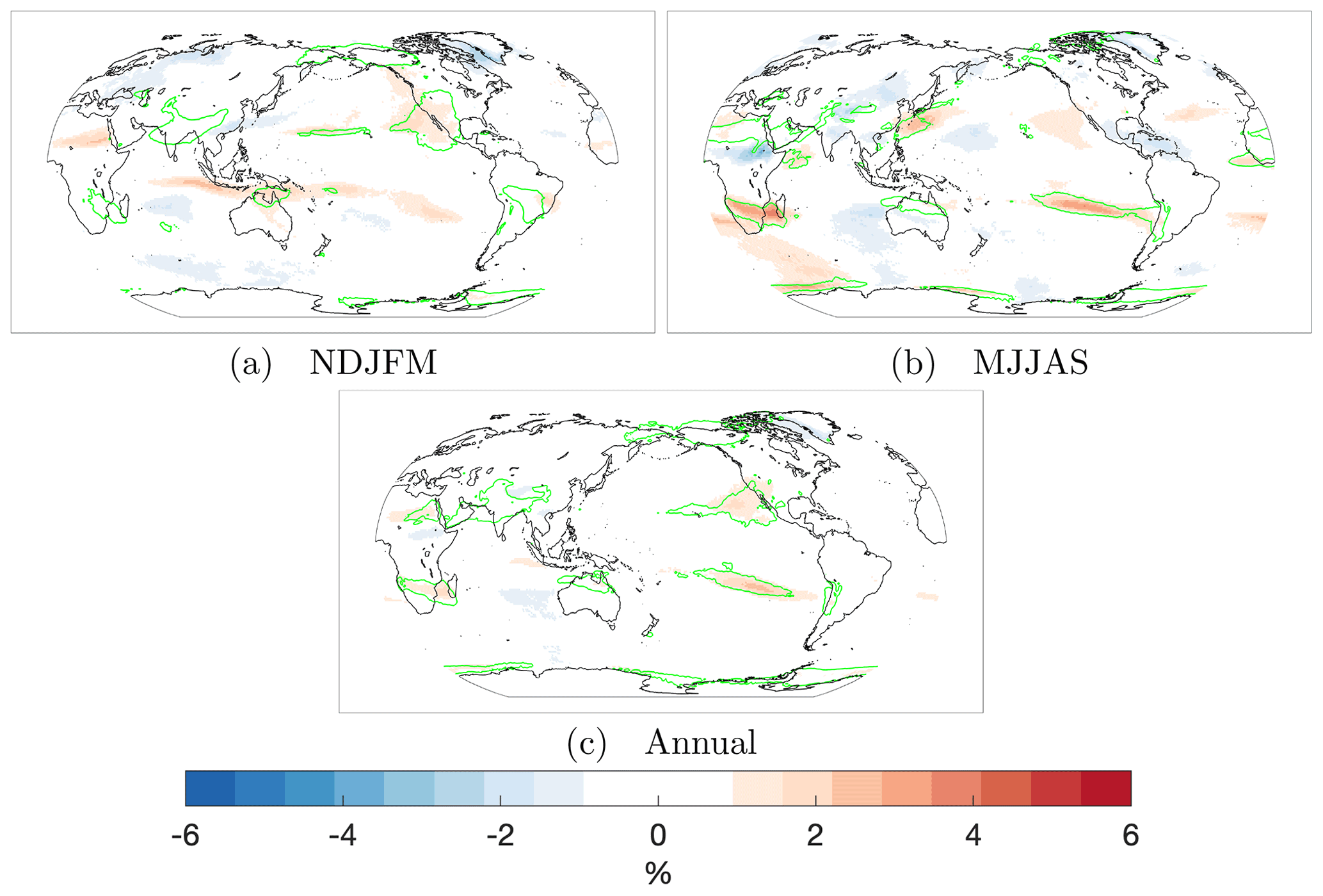
Figure 8Historical ensemble (five members) mean AR frequencies minus AMIP ensemble (three members) mean AR frequencies. Contour lines for the seasonal and annual periods indicate the 2 % and 1.5 % positive AR frequency biases, respectively, from the corresponding biases in Fig. 1c, f, and i.
From examining the major AR biases and large-scale conditions in E3SM regionally and seasonally in the previous sections, we find these features to be most significant: (i) the double ITCZ bias, (ii) a stronger and/or equatorward-shifted subtropical jet during boreal and austral winters, and (iii) stronger westerlies during the Northern Hemisphere summer. As previously mentioned, Dong et al. (2021) found that models with a double ITCZ and associated wetting in the equatorial central Pacific feature an enhanced subtropical jet and weaker mean-state AMOC under global warming. The large-scale anomalies we have uncovered suggest that the double ITCZ bias in E3SM may play a large role in some large-scale circulation biases, such as the subtropical jet bias in North Pacific that contribute to the E3SM AR biases. We look for further evidence by isolating biases in the atmospheric model using the AMIP simulations and comparing them to the fully coupled model for ARs. While atmospheric models may exhibit weak double ITCZ biases, such biases are severely exacerbated in fully coupled models (Zhang et al., 2019). This holds true for E3SM as can be seen in Golaz et al. (2019) Fig. 6b and c, where the fully coupled simulation has a far stronger double ITCZ bias. Thus, by comparing AMIP and coupled simulations, we can determine which biases are common to both simulations – implicating the EAM – or unique to the fully coupled, historical simulation – implicating a coupling response (specifically the double ITCZ response) or other components (e.g., the ocean component or sea ice).
We first compare the ensemble AR frequencies. The AMIP ensemble consists of three members (compared to the five members for the fully coupled ensemble). For context, the AMIP frequencies have slightly better correlations and MAEs (as expected) than the fully coupled ensemble when compared to MERRA2 (e.g., annual ensemble frequency correlation is improved from 0.98 to 0.99 and annual MAE is improved from 0.60 % to 0.54 %). In Fig. 8, we subtract the AMIP ensemble frequencies from the fully coupled ensemble frequencies. Common biases to both ensemble simulations – i.e., regions in Fig. 8 without fully coupled minus AMIP biases (shading) but with fully coupled minus MERRA2 biases (contours) – are the positive AR biases near elevated topography, i.e., the India/Arabian Peninsula, central South America, southeastern Africa, and Alaska/Siberia. This suggests that these biases likely arise from the EAM. Golaz et al. (2019) reported that both AMIP and the fully coupled historical simulations have excessive precipitation over the elevated terrain as well as other precipitation biases.
We also identify several biases that are unique to the fully coupled simulations. Compared to AMIP, the fully coupled simulations have positive AR frequency biases (∼ 3 %) over the Pacific basin and over Africa at subtropical latitudes during the winter season of each hemisphere, suggesting that the wintertime subtropical jet is affected, going from AMIP to fully coupled simulations – particularly on the equatorward flank. During NDJFM, the southwest region of the US and the central North Pacific are zones of enhanced AR frequencies. This is an aforementioned area where the double ITCZ bias response in models deliver excessive moisture (Dong et al., 2021). For the Southern Hemisphere, positive AR frequencies are colocated with the double ITCZ precipitation biases (see Fig. 5c). During MJJAS, the major biases are over the summer rainband region of East Asia, southern Africa, and the eastern subtropical Pacific in the Southern Hemisphere. Given the AR biases over the subtropics in the fully coupled simulation compared to the AMIP simulation, we now examine the changes in the behavior of the subtropical jet between these two simulations.
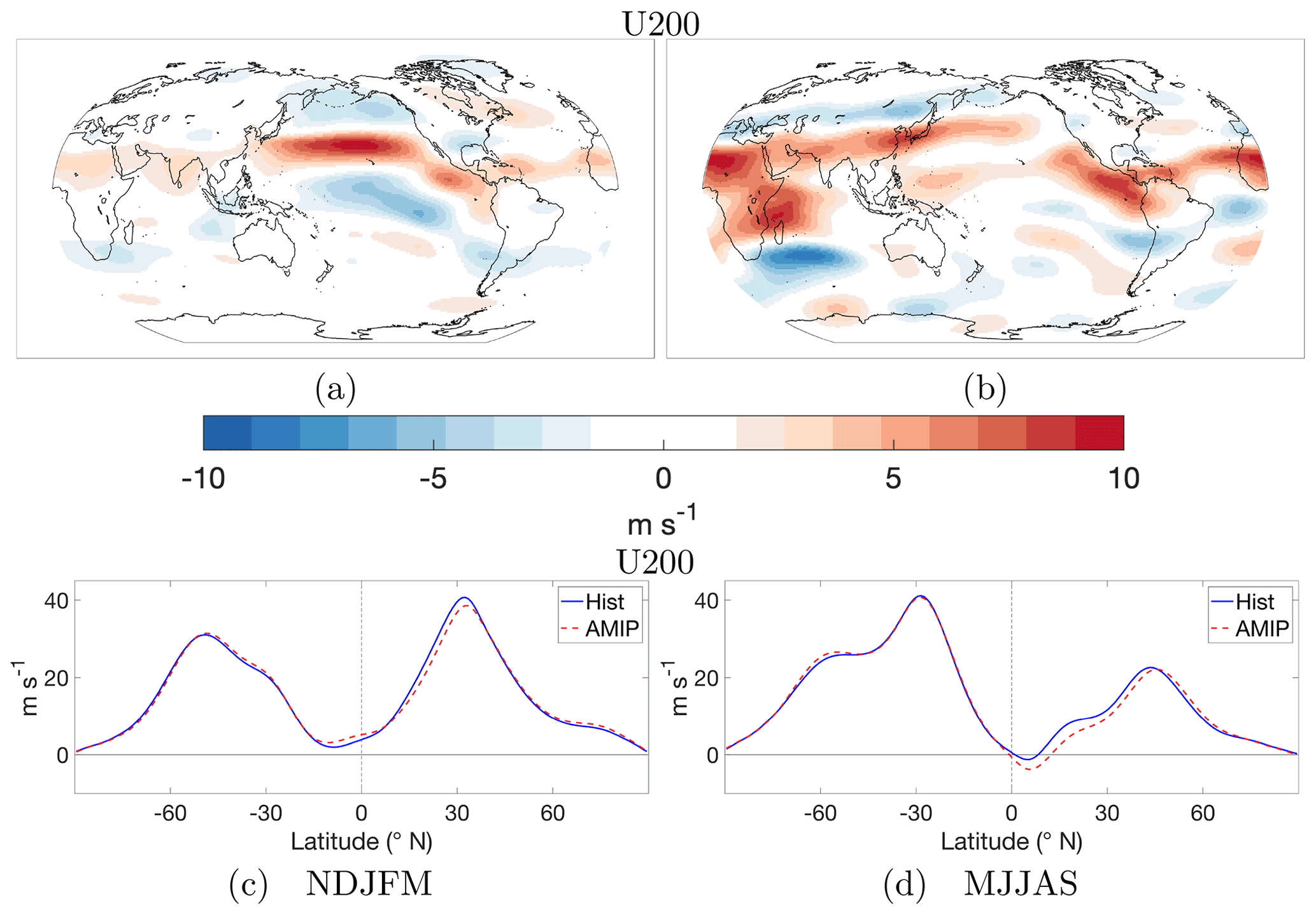
Figure 9Seasonal differences between fully coupled E3SM and AMIP simulations – zonal wind at 200 hPa (a, b) and zonal means over the Pacific and Atlantic basins (100–360∘ E) of zonal wind at 200 hPa (c, d).
In Fig. 9, we compare upper-level zonal winds (zonal wind at 200 hPa) globally for NDJFM and MJJAS. During NDJFM in the Northern Hemisphere, positive upper-level zonal wind anomalies in the fully coupled simulation (Fig. 9a) generally match in location to the anomalies of E3SM compared to MERRA2 (Fig. 7e), while the negative anomalies, particularly over Asia, are weaker. This would suggest that coupling in E3SM is a major source of a stronger, slightly equatorward-shifted, boreal winter subtropical jet. The zonal mean zonal winds (zonally averaged over the Pacific and Atlantic basins) show similar equatorward shifts when comparing the fully coupled simulation to both MERRA2 and AMIP (Figs. 7g and 9c). The Southern Hemisphere differences are generally consistent with MERRA2 differences from the Equator to the subtropics, but the midlatitudes to the polar latitudes lack the southward-shifted, enhanced westerlies over the Southern Ocean/Australia. The enhanced westerlies over this region are a bias common to both fully coupled and AMIP simulations implicating the EAM.
The global MJJAS zonal wind (200 hPa) anomalies between the fully coupled and AMIP simulations qualitatively match the MJJAS anomalies when compared to MERRA2 for most regions. A notable feature is the clear strengthening and southward shift of the subtropical jet seen over subtropical latitudes over much of the Northern Hemisphere – particularly from North Africa moving east to the Pacific basin. The enhanced westerlies over the Tibetan Plateau again correspond with increased AR activity downstream over the East Asian summer rainband region. West of and over southern Africa, there is a band of enhanced westerlies in the fully coupled simulation when compared to both MERRA2 and AMIP (Figs. 7f and 9b). For both of these regions, the evidence points to the biases arising from coupling.
Lastly, we explore what physically causes the jet behavior shifts between fully coupled and AMIP simulations. For NDJFM, the most significant change is a strengthening of the subtropical jet over the North Pacific, and for MJJAS, the enhanced westerlies throughout much of the Northern Hemisphere. Building on the work of Dong et al. (2021), the two significant responses to a double ITCZ bias that the authors uncovered in models, are a strengthened subtropical Pacific jet in projections and a weaker mean-state AMOC in present day. We look for evidence that these responses occur for E3SM going from the AMIP to the fully coupled simulation using upper-troposphere (500–200 hPa) temperatures differences (Fig. 10). Dong et al. (2021) found that due to the double ITCZ, enhanced precipitation over the southern central Pacific generated subtropical changes induced by latent heat release. This leads to enhanced upper-tropospheric warming over the subtropics (Dong et al., 2021 Fig. 2b), which increases the meridional temperature gradient locally, accelerating the subtropical jet along with a southeastward shift of the Aleutian low in projections. We find a similar upper-tropospheric response in temperature over the North Pacific (Fig. 10a); a striking patch of warming occurs in the same area of the subtropical North Pacific with a corresponding cool patch to the north. This enhances the North Pacific wintertime subtropical jet as seen in Fig. 7g.
Dong et al. (2021) also find evidence of weaker present-day AMOC in models with a double ITCZ bias. While the authors focus on the implications for winter precipitation projections over the Mediterranean basin, in this study we examine whether a weaker mean-state AMOC can enhance MJJAS westerlies. The MJJAS response is clearly different than that of the NDJFM response. Figure 10b reveals widespread cold anomalies throughout the Northern Hemisphere, contrasted with some warm anomalies throughout the Southern Hemisphere. The strongest cold anomalies are concentrated in a subtropical/midlatitude band over North Africa, stretching east to East Asia. The strong upper-troposphere cold anomalies at these latitudes increase the meridional temperature gradient, supporting an accelerated summertime subtropical jet. In fact, the band of cold anomalies sits just north of the enhanced subtropical jet anomalies over Africa, Europe, and Asia (Fig. 9b). The hemispheric temperature contrast of a warm Southern Hemisphere and a cold Northern Hemisphere is suggestive of a weaker AMOC (Liu et al., 2020). A weaker AMOC would deliver less cross-equatorial heat to the Northern Hemisphere causing it to be cooler. The weaker AMOC and the double ITCZ are related as a double ITCZ attempts to counteract less northward heat transport with increased northward heat transport via a stronger Southern Hemisphere ITCZ (Zhang et al., 2019).
We also examine the surface air temperature to verify a weaker AMOC in the fully coupled simulation. Specifically, we look for the classic AMOC “fingerprint” which consists primarily of a strong cold temperature anomaly over the subpolar Atlantic Ocean, and, to a lesser degree, as a warm temperature anomaly over the Gulf Stream (Caesar et al., 2018). In Fig. A4, we show surface temperature differences between the fully coupled and AMIP simulations, and find the AMOC “fingerprint” well defined along with a hemispheric contrast in temperature. Liu et al. (2020) isolated the global surface air temperature response to a weakened AMOC and found widespread Northern Hemisphere cooling and more modest Southern Hemisphere warming (Liu et al., 2020 Fig. 2e). This is consistent with Golaz et al. (2019) and Hu et al. (2020), both of which reported a weaker AMOC calculated directly from the ocean model output in the fully coupled E3SM simulation when compared to observations.
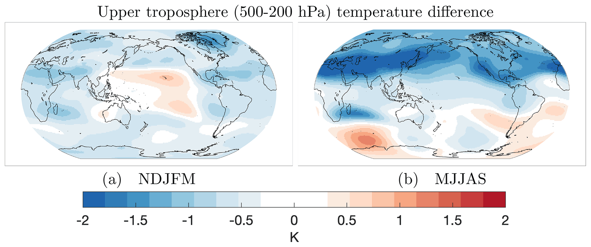
Figure 10Seasonal differences between the fully coupled E3SM and AMIP simulation for upper troposphere (500–200 hPa) temperature.
In this study, we have evaluated E3SM v1.0 at standard resolution for its ability to simulate ARs globally. We compared the fully coupled historical simulation to MERRA2 and began with an examination of global AR frequencies. We find that E3SM is able to simulate ARs with very high degrees of correlation and low MAEs annually (annual correlation 0.98; MAE 0.60 %) and seasonally (NDJFM correlation 0.98; MAE 0.72 %; MJJAS correlation 0.97; MAE 0.82 %). Amongst historical ensemble members, we determined that the internal variability of AR frequencies is low, with the five-member SD under 0.5 % for nearly all grid points. There are however, some biases (most notable when looking at relative differences) such as (i) positive biases occurring near the tropic/subtropical edge during winters of both Northern and Southern hemispheres, (ii) enhanced AR activity over the Middle East, India, and the western boundary of the North Pacific basin during boreal summer, and (iii) on the windward side of the elevated terrain (e.g., Tibetan Plateau). The AR characteristics are compared using probability distributions and we find the E3SM AR characteristics are generally consistent (shape and peak) with MERRA2. Some differences are that the median magnitude of mean AR IVT is higher, and ARs tend to be slightly more zonal in E3SM. The generally higher IVT and stronger westerly jets in E3SM are likely the source of both characteristic differences.
The E3SM distributions of AR precipitation show good agreement with MERRA2, although there is a clear bias resembling the double ITCZ bias and excessive maritime continent precipitation. This manifests as reduced AR precipitation along the equatorial Pacific and excessive AR precipitation just off the Equator in the double ITCZ regions. The AR precipitation fractions reveal a bias in E3SM to attribute excessive precipitation just off the coast of the western US and western Chile as well as over the region near northern Africa/the Middle East/India.
An examination of the large-scale conditions relevant to ARs in E3SM reveals these features to be most significant in producing AR biases in E3SM: (i) the double ITCZ bias, (ii) a stronger and/or equatorward-shifted subtropical jet during boreal and austral winters, and (iii) enhanced westerlies during the Northern Hemisphere summer. The work of Dong et al. (2021) showed that there is a significant relationship in models with a present-day double ITCZ bias to have a stronger projected North Pacific subtropical jet as well as a weaker present-day AMOC. Given the clear double ITCZ bias in the fully coupled E3SM, we investigated whether the interconnected processes of the North Pacific jet, Aleutian low, and AMOC with a double ITCZ were present in the E3SM historical simulation, and if they could explain AR biases. Analysis of the E3SM large-scale circulation biases identified biases in the subtropical jet during both NDJFM and MJJAS that could contribute to the AR precipitation biases. The strengthened and slightly equatorward-shifted North Pacific jet, and the impact on AR precipitation in the Southwest US, is consistent with the signature identified by Dong et al. (2021) as related to the double ITCZ during winter.
Motivated by the analysis of large-scale circulation biases and their general correspondence with the AR precipitation bias, we further compared the fully coupled (strong double ITCZ bias) and AMIP simulations (no-to-weak double ITCZ bias) to isolate the changes that occur when moving from an atmosphere-only model to a fully coupled model, while specifically looking for evidence of a stronger subtropical jet and weaker AMOC. The analysis suggests that the AR frequency biases over the elevated terrain, i.e., the India/Arabian Peninsula, central South America, and Alaska/Siberia, can be attributed to the EAM, as similar biases are found in both AMIP and coupled simulations. Biases arising from coupling or other model components include the positive AR frequencies over the North Pacific subtropics and southwestern region of the US during NDJFM, and over the East Asian summer rainband region and the Southern Hemisphere's eastern subtropical Pacific during MJJAS. These coupling biases suggest that the model responses to a double ITCZ revealed in Dong et al. (2021) could be the source even in present-day simulations. We show evidence that the physical processes leading to a stronger North Pacific subtropical jet during NDJFM and enhanced Northern Hemisphere westerlies during MJJAS are consistent with Dong et al. (2021). The North Pacific subtropical jet is enhanced via increased, upper-troposphere temperature gradients, generated through teleconnections induced by enhanced heat release in the equatorial Pacific Ocean, related to the double ITCZ. Reducing the double ITCZ bias remains an open issue in modeling, but previous studies suggest that improvements to parameterizations of boundary-layer turbulence and convective schemes can reduce this bias (e.g., Song and Zhang, 2018; Lu et al., 2021), which in turn could improve the water vapor transport and AR biases seen in E3SM as well as other GCMs.
On the other hand, the enhanced Northern Hemisphere westerlies during summer are due to a band of strong cold anomalies in the upper-troposphere, stretching east from North Africa to East Asia. The upper-troposphere temperature differences reveal a hemispheric temperature contrast with a cool Northern Hemisphere and warm Southern Hemisphere bias – suggestive of a weaker AMOC. We find that the fully coupled simulation does indeed have a weaker mean-state AMOC, evidenced by the AMOC “fingerprint” in surface temperature comparisons, which is consistent with the weak AMOC reported by Golaz et al. (2019) and Hu et al. (2020), based on analysis of the ocean circulation in the coupled simulations.
We note, however, that the cold bias in the Northern Hemisphere and the opposite bias in the Southern Hemisphere may also be contributed by the strong model response to aerosol forcings, as found by Golaz et al. (2019). Aerosol forcing is strongest over the Northern Hemisphere midlatitudes (Hansen et al., 1998; Ma et al., 2012; Friedman et al., 2013) during spring through summer, and during MJJAS is indeed when we see the strongest signal in cold anomalies. Another contributing factor for the interhemispheric temperature contrast could be from the delayed warming – related to E3SM's strong aerosol forcing – in the coupled historical simulation between 1960–1990, which keeps the global surface air temperature lower than observations until about 2010. The long period of delayed warming could reduce the interhemispheric temperature asymmetry signal from climate change, which has amplified warming of the Northern Hemisphere (Friedman et al., 2013). The cool Northern and warm Southern Hemisphere biases in the coupled E3SM simulation may also explain why the Northern Hemisphere's jet strengthening and shift is more significant than the Southern Hemisphere during MJJAS, as the upper-level temperature gradients are increased and decreased over the subtropical latitudes for the Northern and Southern hemispheres, respectively. More generally, biases in the subtropical jet in E3SM may be contributed by other sources of model biases besides the double ITCZ and related weak AMOC. Future analysis including the high-resolution E3SM simulation (Caldwell et al., 2019) may offer additional insights on AR and large-scale circulation biases, as AMOC is noticeably stronger at high resolution compared to the low-resolution simulations analyzed here.
This study not only provides a comprehensive, global overview of AR representation in the fully coupled historical E3SM v1.0 simulation that should give users of E3SM confidence in its ability to realistically simulate ARs but also seeks to understand how and why some biases are present. While we have framed this analysis through the lens of ARs, the biases in large-scale conditions are relevant to other phenomena and also provide potential areas of improvement in the EAM and the fully coupled simulations. Evaluating AR frequency biases in other CMIP5/6 GCMs to reanalysis, such as those used in O’Brien et al. (2021), suggests that the AR biases associated with a double ITCZ may be more general than found in E3SM alone. Analysis of the high-resolution simulation and future projections by E3SM is useful to further understand model biases and their implications for projecting future changes in AR frequency, intensity, and extreme precipitation.
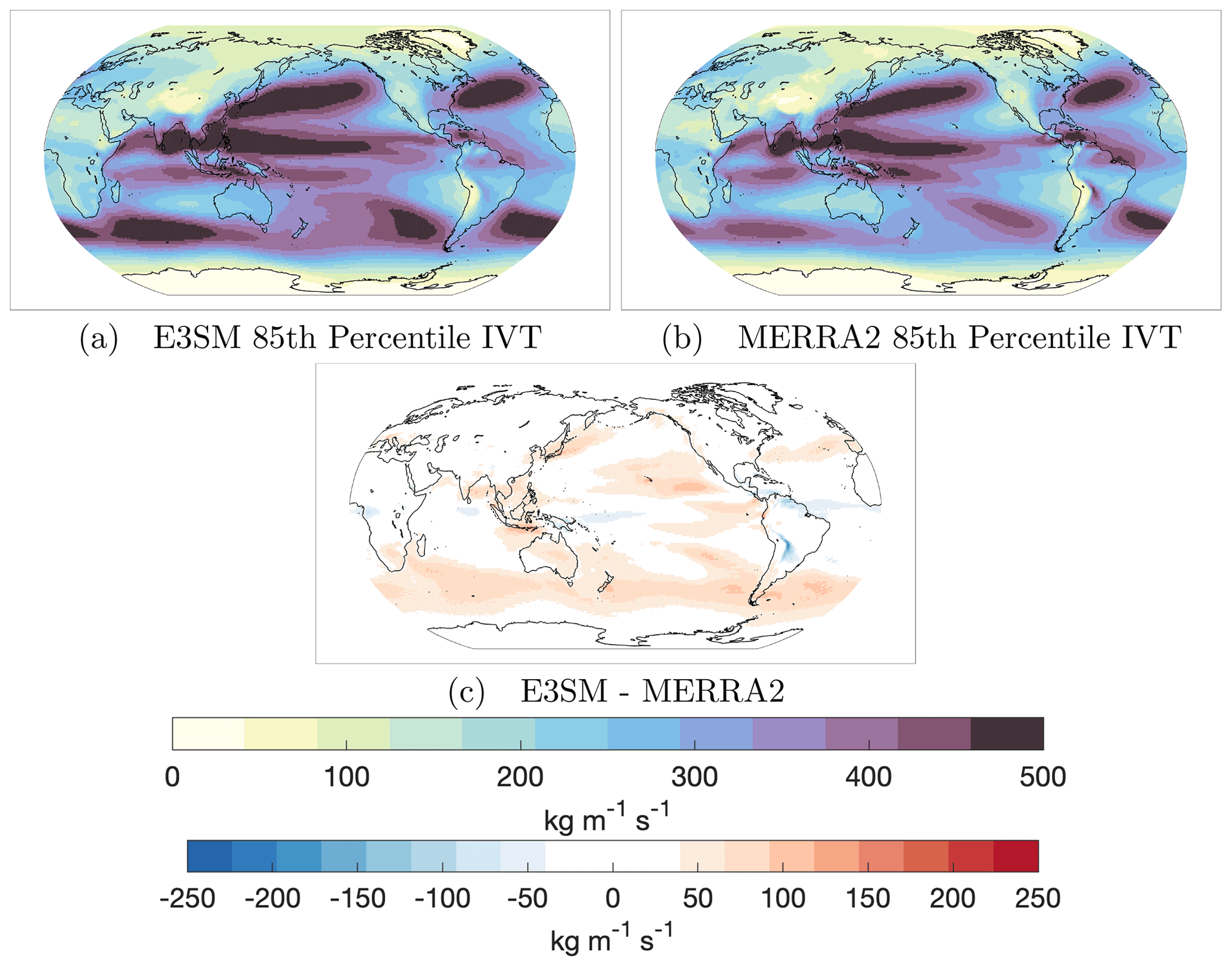
Figure A1Annual mean 85th percentile IVT for (a) E3SM and (b) MERRA2. The difference (E3SM minus MERRA2) is shown in (c).
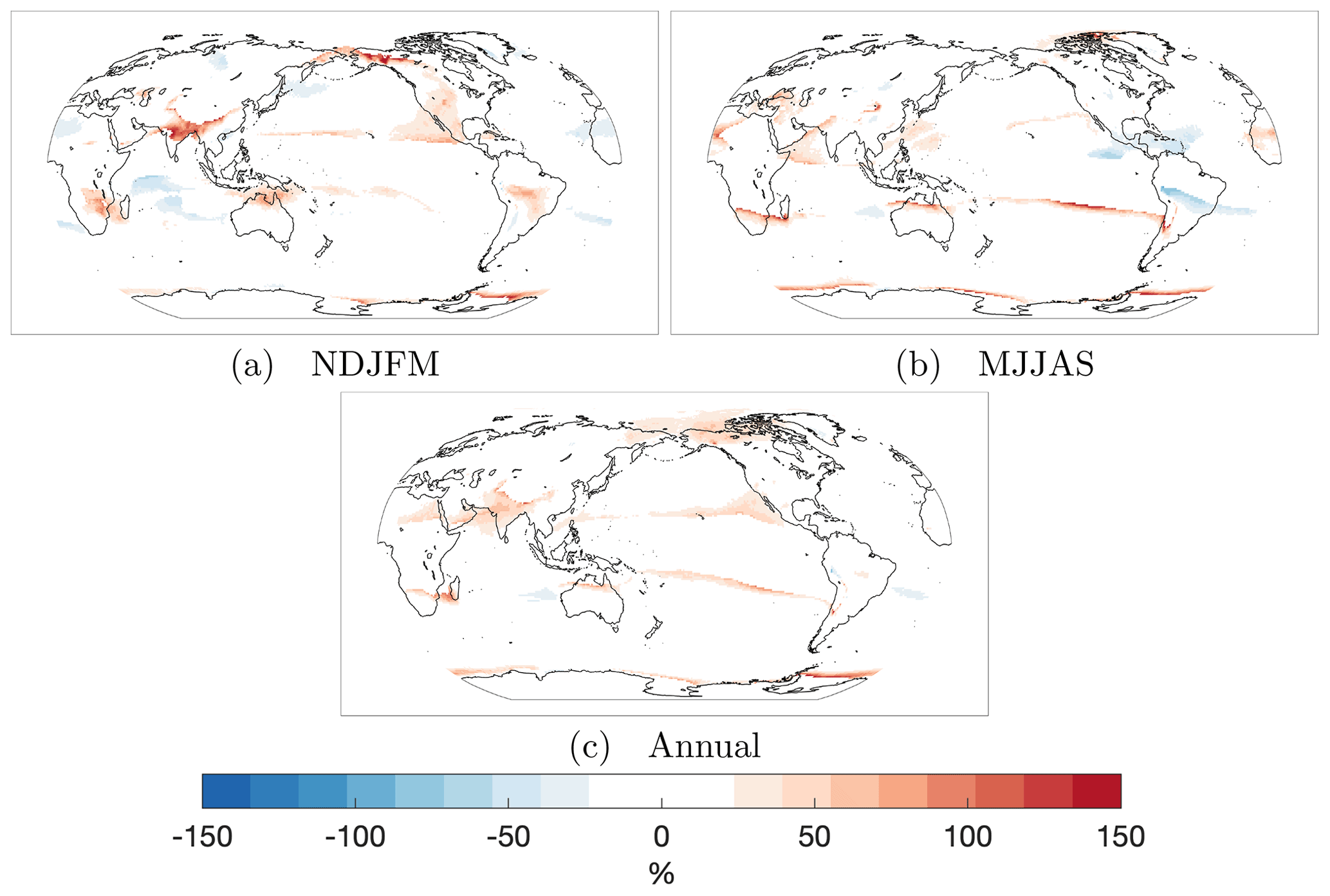
Figure A2The AR relative frequency differences (as opposed to absolute frequency differences) by percentage corresponding with Fig. 1c, f, and i. Only grid points with MERRA2 AR frequencies (absolute) of at least 3 % are shown (regions with very low AR frequencies can show relative differences of 100 % due to a single extra time step).
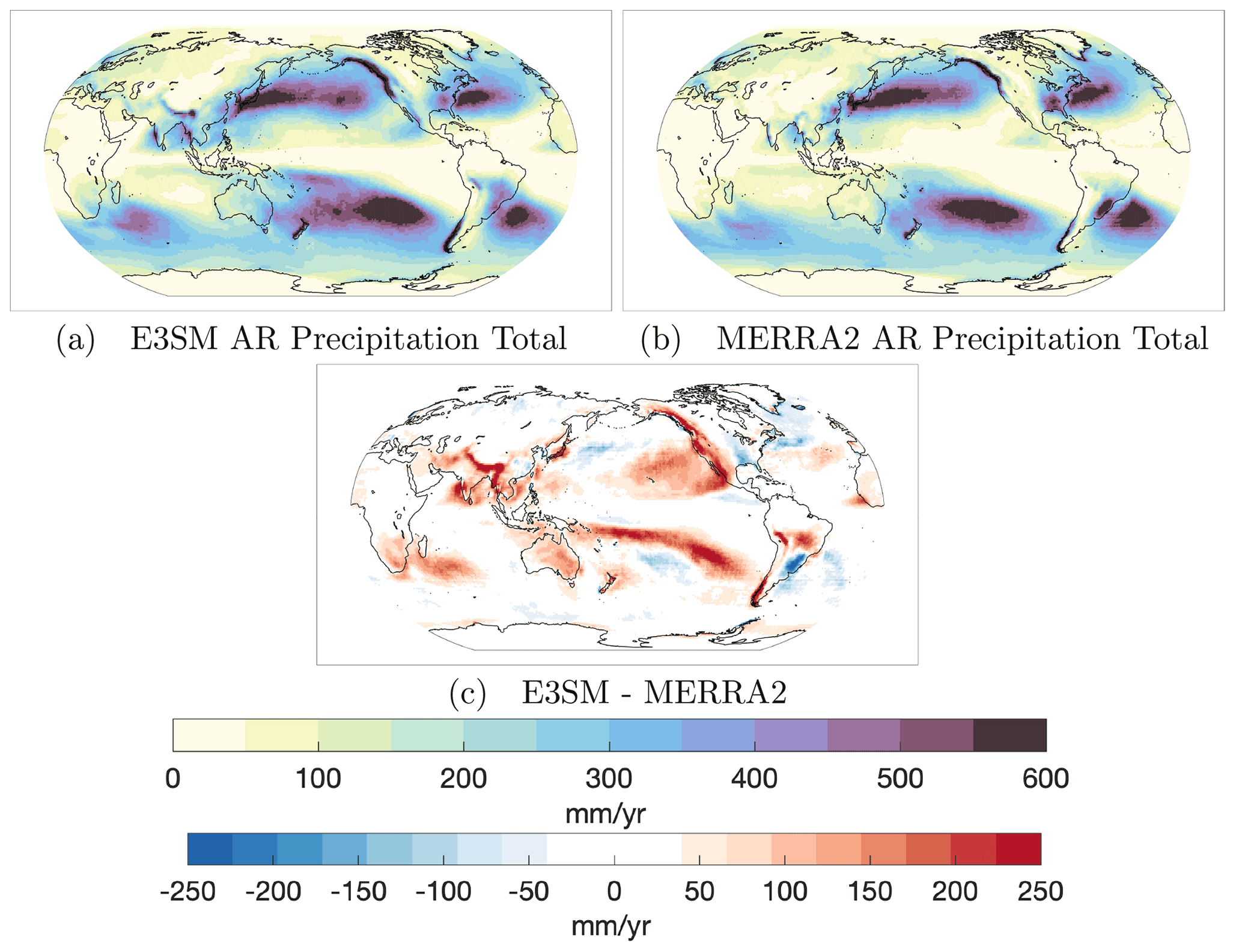
Figure A3Mean annual total AR precipitation for (a) E3SM and (b) MERRA2. The difference is shown in (c).
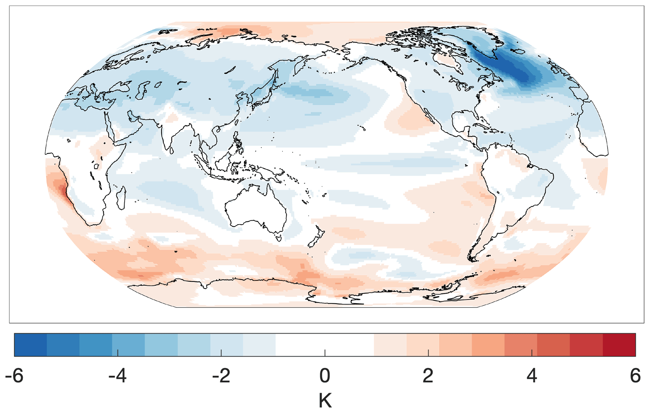
Figure A4Annual surface temperature differences between the fully coupled E3SM simulation and the AMIP E3SM simulation.
The E3SM and MERRA2 datasets used in this study are publicly available at https://esgf-node.llnl.gov/projects/e3sm/ (E3SM Project and DOE, 2018) and https://disc.gsfc.nasa.gov/datasets?project=MERRA-2 (last access: 14 September 2021), respectively (DOI: https://doi.org/10.5067/VJAFPLI1CSIV, GMAO, 2015a; https://doi.org/10.5067/QBZ6MG944HW0, GMAO, 2015b; https://doi.org/10.5067/7MCPBJ41Y0K6, GMAO, 2015c; https://doi.org/10.5067/Q5GVUVUIVGO7, GMAO, 2015d). The tARget v3 algorithm is available at https://doi.org/10.25346/S6/B89KXF (Guan, 2021).
SK and LRL conceived the project idea and plan. SK, LRL, and JCHC contributed to the investigation and design of the methodology. BG provided the tARget v3 atmospheric river detection algorithm software and provided support to SK on applying it. LRL and JCHC both supervised SK throughout the project. All authors contributed to the writing and reviewing of the manuscript. SK performed the formal analysis and created the visualizations.
The contact author has declared that neither they nor their co-authors have any competing interests.
Publisher’s note: Copernicus Publications remains neutral with regard to jurisdictional claims in published maps and institutional affiliations.
Sol Kim and L. Ruby Leung were supported by the Office of Science, US Department of Energy Biological and Environmental Research, as part of the Regional and Global Model Analysis program area. We acknowledge National Energy Research Scientific Computing Center (NERSC), a US Department of Energy Office of Science User Facility located at Lawrence Berkeley National Laboratory, operated under contract no. DE-AC02-05CH11231, for the allocation of computational resources which enabled us to perform the data analysis. The Pacific Northwest National Laboratory (PNNL) is operated for the Department of Energy by Battelle Memorial Institute under contract DE-AC05-76RL01830.
This research has been supported by the US Department of Energy, Office of Science (grant no. KP1703010).
This paper was edited by Richard Neale and reviewed by two anonymous referees.
Caesar, L., Rahmstorf, S., Robinson, A., Feulner, G., and Saba, V.: Observed fingerprint of a weakening Atlantic Ocean overturning circulation, Nature, 556, 191–196, 2018. a
Caldwell, P. M., Mametjanov, A., Tang, Q., Van Roekel, L. P., Golaz, J.-C., Lin, W., Bader, D. C., Keen, N. D., Feng, Y., Jacob, R., et al.: The DOE E3SM coupled model version 1: Description and results at high resolution, J. Adv. Model. Earth Sy., 11, 4095–4146, 2019. a
Chen, X., Leung, L. R., Wigmosta, M., and Richmond, M.: Impact of atmospheric rivers on surface hydrological processes in western US watersheds, J. Geophys. Res.-Atmos., 124, 8896–8916, 2019. a
Chiang, J. C., Fischer, J., Kong, W., and Herman, M. J.: Intensification of the pre-Meiyu rainband in the late 21st century, Geophys. Res. Lett., 46, 7536–7545, 2019. a
Corringham, T. W., Ralph, F. M., Gershunov, A., Cayan, D. R., and Talbot, C. A.: Atmospheric rivers drive flood damages in the western United States, Science Advances, 5, eaax4631, https://doi.org/10.1126/sciadv.aax4631, 2019. a
DeFlorio, M. J., Waliser, D. E., Guan, B., Ralph, F. M., and Vitart, F.: Global evaluation of atmospheric river subseasonal prediction skill, Clim. Dynam., 52, 3039–3060, 2019. a
Dettinger, M. D., Ralph, F. M., Das, T., Neiman, P. J., and Cayan, D. R.: Atmospheric rivers, floods and the water resources of California, Water, 3, 445–478, 2011. a
Dong, L., Leung, L. R., Lu, J., and Song, F.: Double-ITCZ as an emergent constraint for future precipitation over Mediterranean climate regions in the North Hemisphere, Geophys. Res. Lett., 48, e2020GL091569, https://doi.org/10.1029/2020GL091569, 2021. a, b, c, d, e, f, g, h, i, j, k, l, m, n
E3SM Project and DOE: Energy Exascale Earth System Model v1.0, DOE Code [data set], https://doi.org/10.11578/E3SM/dc.20180418.36, 2018. a
Espinoza, V., Waliser, D. E., Guan, B., Lavers, D. A., and Ralph, F. M.: Global analysis of climate change projection effects on atmospheric rivers, Geophys. Res. Lett., 45, 4299–4308, 2018. a, b
Eyring, V., Bony, S., Meehl, G. A., Senior, C. A., Stevens, B., Stouffer, R. J., and Taylor, K. E.: Overview of the Coupled Model Intercomparison Project Phase 6 (CMIP6) experimental design and organization, Geosci. Model Dev., 9, 1937–1958, https://doi.org/10.5194/gmd-9-1937-2016, 2016. a
Friedman, A. R., Hwang, Y.-T., Chiang, J. C., and Frierson, D. M.: Interhemispheric temperature asymmetry over the twentieth century and in future projections, J. Climate, 26, 5419–5433, 2013. a, b
Gelaro, R., McCarty, W., Suárez, M. J., Todling, R., Molod, A., Takacs, L., Randles, C. A., Darmenov, A., Bosilovich, M. G., Reichle, R., et al.: The modern-era retrospective analysis for research and applications, version 2 (MERRA-2), J. Climate, 30, 5419–5454, 2017. a
Global Modeling and Assimilation Office (GMAO): MERRA-2 tavg1_2d_slv_Nx: 2d,1-Hourly, Time-Averaged, Single-Level, Assimilation, Single-Level Diagnostics V5.12.4, Greenbelt, MD, USA, Goddard Earth Sciences Data and Information Services Center (GES DISC) [data set], https://doi.org/10.5067/VJAFPLI1CSIV, 2015a. a
Global Modeling and Assimilation Office (GMAO): MERRA-2 inst3_3d_asm_Np: 3d, 3-Hourly, Instantaneous, Pressure-Level, Assimilation, Assimilated Meteorological Fields V5.12.4, Greenbelt, MD, USA, Goddard Earth Sciences Data and Information Services Center (GES DISC) [data set], https://doi.org/10.5067/QBZ6MG944HW0, 2015b. a
Global Modeling and Assimilation Office (GMAO): MERRA-2 tavg1_2d_flx_Nx: 2d, 1-Hourly, Time-Averaged, Single-Level, Assimilation, Surface Flux Diagnostics V5.12.4, Greenbelt, MD, USA, Goddard Earth Sciences Data and Information Services Center (GES DISC) [data set], https://doi.org/10.5067/7MCPBJ41Y0K6, 2015c. a
Global Modeling and Assimilation Office (GMAO): MERRA-2 tavg1_2d_int_Nx: 2d, 1-Hourly, Time-Averaged, Single-Level, Assimilation, Vertically Integrated Diagnostics V5.12.4, Greenbelt, MD, USA, Goddard Earth Sciences Data and Information Services Center (GES DISC) [data set], https://doi.org/10.5067/Q5GVUVUIVGO7, 2015d. a
Golaz, J.-C., Caldwell, P. M., Van Roekel, L. P., Petersen, M. R., Tang, Q., Wolfe, J. D., Abeshu, G., Anantharaj, V., Asay-Davis, X. S., Bader, D. C., et al.: The DOE E3SM coupled model version 1: Overview and evaluation at standard resolution, J. Adv. Model. Earth Sy., 11, 2089–2129, 2019. a, b, c, d, e, f, g, h, i, j, k, l, m
Guan, B.: Tracking Atmospheric Rivers Globally as Elongated Targets (tARget), Version 3, UCLA Dataverse [code], https://doi.org/10.25346/S6/B89KXF, 2021. a
Guan, B. and Waliser, D. E.: Detection of atmospheric rivers: Evaluation and application of an algorithm for global studies, J. Geophys. Res.-Atmos., 120, 12514–12535, 2015. a, b, c, d, e, f, g
Guan, B. and Waliser, D. E.: Atmospheric rivers in 20 year weather and climate simulations: A multimodel, global evaluation, J. Geophys. Res.-Atmos., 122, 5556–5581, 2017. a
Guan, B. and Waliser, D. E.: Tracking Atmospheric Rivers Globally: Spatial Distributions and Temporal Evolution of Life Cycle Characteristics, J. Geophys. Res.-Atmos., 124, 12523–12552, https://doi.org/10.1029/2019JD031205, 2019. a, b, c
Guan, B., Waliser, D. E., and Ralph, F. M.: An intercomparison between reanalysis and dropsonde observations of the total water vapor transport in individual atmospheric rivers, J. Hydrometeorol., 19, 321–337, 2018. a, b, c, d, e
Hagos, S. M., Leung, L. R., Yoon, J.-H., Lu, J., and Gao, Y.: A projection of changes in landfalling atmospheric river frequency and extreme precipitation over western North America from the Large Ensemble CESM simulations, Geophys. Res. Lett., 43, 1357–1363, 2016. a
Hansen, J. E., Sato, M., Lacis, A., Ruedy, R., Tegen, I., and Matthews, E.: Climate forcings in the industrial era, P. Natl. Acad. Sci. USA, 95, 12753–12758, 1998. a
Hu, A., Van Roekel, L., Weijer, W., Garuba, O. A., Cheng, W., and Nadiga, B. T.: Role of AMOC in transient climate response to greenhouse gas forcing in two coupled models, J. Climate, 33, 5845–5859, 2020. a, b
Leung, L. R., Bader, D. C., Taylor, M. A., and McCoy, R. B.: An introduction to the E3SM special collection: Goals, science drivers, development, and analysis, J. Adv. Model. Earth Sy., 12, e2019MS001821, https://doi.org/10.1029/2019MS001821, 2020. a, b
Li, G. and Xie, S.-P.: Origins of tropical-wide SST biases in CMIP multi-model ensembles, Geophys. Res. Lett., 39, L22703, https://doi.org/10.1029/2012GL053777, 2012. a
Li, G. and Xie, S.-P.: Tropical biases in CMIP5 multimodel ensemble: The excessive equatorial Pacific cold tongue and double ITCZ problems, J. Climate, 27, 1765–1780, 2014. a
Liu, W., Fedorov, A. V., Xie, S.-P., and Hu, S.: Climate impacts of a weakened Atlantic Meridional Overturning Circulation in a warming climate, Science Advances, 6, eaaz4876, https://doi.org/10.1126/sciadv.aaz4876, 2020. a, b, c
Lu, Y., Wu, T., Li, Y., and Yang, B.: Mitigation of the double ITCZ syndrome in BCC-CSM2-MR through improving parameterizations of boundary-layer turbulence and shallow convection, Geosci. Model Dev., 14, 5183–5204, https://doi.org/10.5194/gmd-14-5183-2021, 2021. a
Ma, X., Yu, F., and Luo, G.: Aerosol direct radiative forcing based on GEOS-Chem-APM and uncertainties, Atmos. Chem. Phys., 12, 5563–5581, https://doi.org/10.5194/acp-12-5563-2012, 2012. a
O’Brien, T. A., Payne, A. E., Shields, C. A., Rutz, J., Brands, S., Castellano, C., Chen, J., Cleveland, W., DeFlorio, M. J., Goldenson, N., et al.: Detection uncertainty matters for understanding atmospheric rivers, B. Am. Meteorol. Soc., 101, E790–E796, 2020. a
O’Brien, T. A., Wehner, M. F., Payne, A. E., Shields, C. A., Rutz, J. J., Leung, L.-R., Ralph, F. M., Collow, A., Gorodetskaya, I., Guan, B., J. Lora, M., McClenny, E., Nardi, K. M., Ramos, A. M., Tomé, R., Sarangi, C., Shearer, E. J., Ullrich, P. A., Zarzycki, C., Loring, B., Huang, H., Inda-Díaz, H. A., Rhoades, A. M., and Zhou, Y.: Increases in future AR count and size: Overview of the ARTMIP Tier 2 CMIP5/6 experiment, J. Geophys. Res.-Atmos., 127, e2021JD036013, https://doi.org/10.1029/2021JD036013, 2021. a, b, c
Payne, A. E. and Magnusdottir, G.: An evaluation of atmospheric rivers over the North Pacific in CMIP5 and their response to warming under RCP 8.5, J. Geophys. Res.-Atmos., 120, 11–173, 2015. a, b, c
Payne, A. E., Demory, M.-E., Leung, L. R., Ramos, A. M., Shields, C. A., Rutz, J. J., Siler, N., Villarini, G., Hall, A., and Ralph, F. M.: Responses and impacts of atmospheric rivers to climate change, Nature Reviews Earth & Environment, 1, 143–157, https://doi.org/10.1038/s43017-020-0030-5, 2020. a
Ralph, F., Wick, G., Neiman, P., Moore, B., Spackman, J., Hughes, M., Yong, F., and Hock, T.: Atmospheric rivers in reanalysis products: A six-event comparison with aircraft observations of water vapor transport, in: Extended abstracts, WCRP Reanalysis Conf., Silver Spring, MD, https://www.wcrp-climate.org/ICR4/posters/Hughes_AT-20.pdf (last access: 2 June 2021), 2012. a
Ralph, F. M., Neiman, P. J., and Wick, G. A.: Satellite and CALJET aircraft observations of atmospheric rivers over the eastern North Pacific Ocean during the winter of 1997/98, Mon. Weather Rev., 132, 1721–1745, 2004. a
Ralph, F. M., Neiman, P. J., and Rotunno, R.: Dropsonde observations in low-level jets over the northeastern Pacific Ocean from CALJET-1998 and PACJET-2001: Mean vertical-profile and atmospheric-river characteristics, Mon. Weather Rev., 133, 889–910, 2005. a
Ralph, F. M., Neiman, P. J., Wick, G. A., Gutman, S. I., Dettinger, M. D., Cayan, D. R., and White, A. B.: Flooding on California's Russian River: Role of atmospheric rivers, Geophys. Res. Lett., 33, L13801, https://doi.org/10.1029/2006GL026689, 2006. a
Ralph, F. M., Rutz, J. J., Cordeira, J. M., Dettinger, M., Anderson, M., Reynolds, D., Schick, L. J., and Smallcomb, C.: A scale to characterize the strength and impacts of atmospheric rivers, B. Am. Meteorol. Soc., 100, 269–289, 2019. a
Ralph, F. M., Dettinger, M. D., Rutz, J. J., and Waliser, D. E.: Atmospheric Rivers, 1st edn., vol. 1, Springer, ISBN 978-3-030-28906-5, https://doi.org/10.1007/978-3-030-28906-5, 2020. a, b, c, d
Rasch, P., Xie, S., Ma, P.-L., Lin, W., Wang, H., Tang, Q., Burrows, S., Caldwell, P., Zhang, K., Easter, R., et al.: An overview of the atmospheric component of the Energy Exascale Earth System Model, J. Adv. Model. Earth Sy., 11, 2377–2411, 2019. a, b
Rutz, J. J., Shields, C. A., Lora, J. M., Payne, A. E., Guan, B., Ullrich, P., O’Brien, T., Leung, L. R., Ralph, F. M., Wehner, M., et al.: The Atmospheric River Tracking Method Intercomparison Project (ARTMIP): Quantifying Uncertainties in Atmospheric River Climatology, J. Geophys. Res.-Atmos., 124, 13777–13802, https://doi.org/10.1029/2019JD030936, 2019. a, b
Shields, C. A. and Kiehl, J. T.: Atmospheric river landfall-latitude changes in future climate simulations, Geophys. Res. Lett., 43, 8775–8782, 2016. a, b
Shields, C. A., Rutz, J. J., Leung, L.-Y., Ralph, F. M., Wehner, M., Kawzenuk, B., Lora, J. M., McClenny, E., Osborne, T., Payne, A. E., Ullrich, P., Gershunov, A., Goldenson, N., Guan, B., Qian, Y., Ramos, A. M., Sarangi, C., Sellars, S., Gorodetskaya, I., Kashinath, K., Kurlin, V., Mahoney, K., Muszynski, G., Pierce, R., Subramanian, A. C., Tome, R., Waliser, D., Walton, D., Wick, G., Wilson, A., Lavers, D., Prabhat, Collow, A., Krishnan, H., Magnusdottir, G., and Nguyen, P.: Atmospheric River Tracking Method Intercomparison Project (ARTMIP): project goals and experimental design, Geosci. Model Dev., 11, 2455–2474, https://doi.org/10.5194/gmd-11-2455-2018, 2018. a, b, c
Shields, C. A., Rutz, J. J., Leung, L. R., Ralph, F. M., Wehner, M., O’Brien, T., and Pierce, R.: Defining uncertainties through comparison of atmospheric river tracking methods, B. Am. Meteorol. Soc., 100, ES93–ES96, 2019. a
Song, X. and Zhang, G. J.: The roles of convection parameterization in the formation of double ITCZ syndrome in the NCAR CESM: I. Atmospheric processes, J. Adv. Model. Earth Sy., 10, 842–866, 2018. a
Swain, D. L., Langenbrunner, B., Neelin, J. D., and Hall, A.: Increasing precipitation volatility in twenty-first-century California, Nat. Clim. Change, 8, 427–433, 2018. a
Wahl, E. R., Zorita, E., Trouet, V., and Taylor, A. H.: Jet stream dynamics, hydroclimate, and fire in California from 1600 CE to present, P. Natl. Acad. Sci. USA, 116, 5393–5398, 2019. a
Warner, M. D., Mass, C. F., and Salathe Jr, E. P.: Changes in winter atmospheric rivers along the North American west coast in CMIP5 climate models, J. Hydrometeorol., 16, 118–128, 2015. a
Zhang, G. J., Song, X., and Wang, Y.: The double ITCZ syndrome in GCMs: A coupled feedback problem among convection, clouds, atmospheric and ocean circulations, Atmos. Res., 229, 255–268, 2019. a, b
Zhang, W. and Villarini, G.: Uncovering the role of the East Asian jet stream and heterogeneities in atmospheric rivers affecting the western United States, P. Natl. Acad. Sci. USA, 115, 891–896, 2018. a
Zhang, X., Lin, W., and Zhang, M.: Toward understanding the double Intertropical Convergence Zone pathology in coupled ocean-atmosphere general circulation models, J. Geophys. Res.-Atmos., 112, D12102, https://doi.org/10.1029/2006JD007878, 2007. a
Zhu, Y. and Newell, R. E.: A proposed algorithm for moisture fluxes from atmospheric rivers, Mon. Weather Rev., 126, 725–735, 1998. a